Deconstructing Data ScienceDavid Bamman, UC Berkeley

Info 290

Lecture 7: Decision trees & random forests

Feb 10, 2016

Logistic regression

Support vector machines

Ordinal regression

Linear regression

Topic models

Probabilistic graphical models

Survival models

Networks

Perceptron

Neural networks

Deep learning

K-means clustering

Hierarchical clustering

Decision trees

Random forests

Decision trees

Random forests

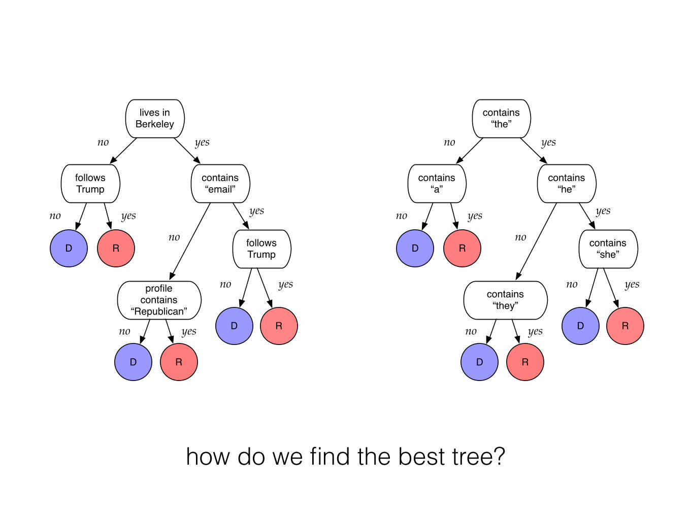
20 questions

lives in Berkeley

follows Trump

contains “email”

profile contains

“Republican”

follows Trump

RD

RD

RD

yes

yes

yes

no

no

no

no

no yes

yes

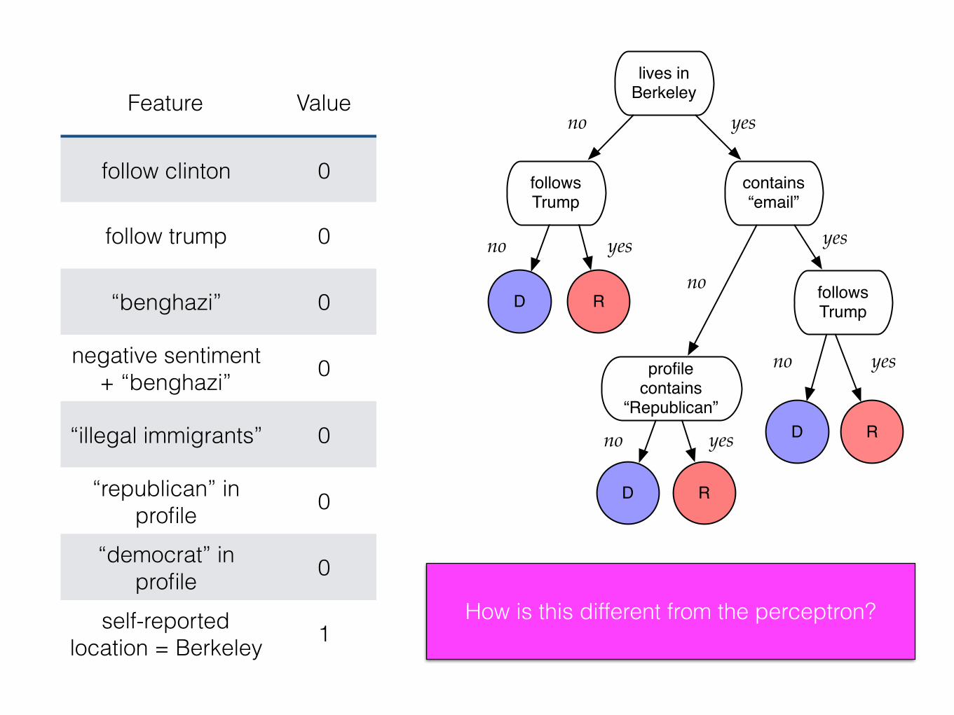
Feature Value

follow clinton 0

follow trump 0

“benghazi” 0

negative sentiment + “benghazi” 0

“illegal immigrants” 0

“republican” in profile 0

“democrat” in profile 0

self-reported location = Berkeley 1

lives in Berkeley

follows Trump

contains “email”

profile contains

“Republican”

follows Trump

RD

RD

RD

yes

yes

yes

no

no

no

no

no yes

yes

contains “the”

contains “a”

contains “he”

contains “they”

contains “she”

RD

RD

RD

yes

yes

yes

no

no

no

no

no yes

yes

how do we find the best tree?

contains “the”

contains “a”

contains “he”

contains “they”

contains “she”

RD

RD

RD

yes

yes

yes

no

no

no

no

no yes

yes

how do we find the best tree?

…

contains “the”

contains “a”

contains “he”

contains “they”

contains “she”RD

yes

yes

no

no

no yes

contains “an”

contains”are”

contains “our”

contains “them”

contains “him”

RD

RD

yes

yes

yes

no

no

no

no

no yes

yes

…

…

contains “her”

contains “hers”

contains “his”

R

RD

yes

no

yes

…

D

no

yes

Decision trees

from Flach 2014

<x, y>training data

x1 > 10x1 ≤ 10

x2 >15

x2 ≤ 15

x2 > 5

x2 ≤ 5

Decision trees

from Flach 2014

• Homogeneous(D): the elements in D are homogeneous enough that they can be labeled with a single label

• Label(D): the single most appropriate label for all elements in D

Decision trees

Decision trees

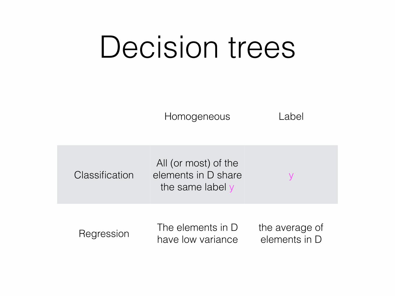
Homogeneous Label

ClassificationAll (or most) of the

elements in D share the same label y

y

Regression The elements in D have low variance

the average of elements in D

Decision trees

from Flach 2014

Measure of uncertainty in a probability distribution

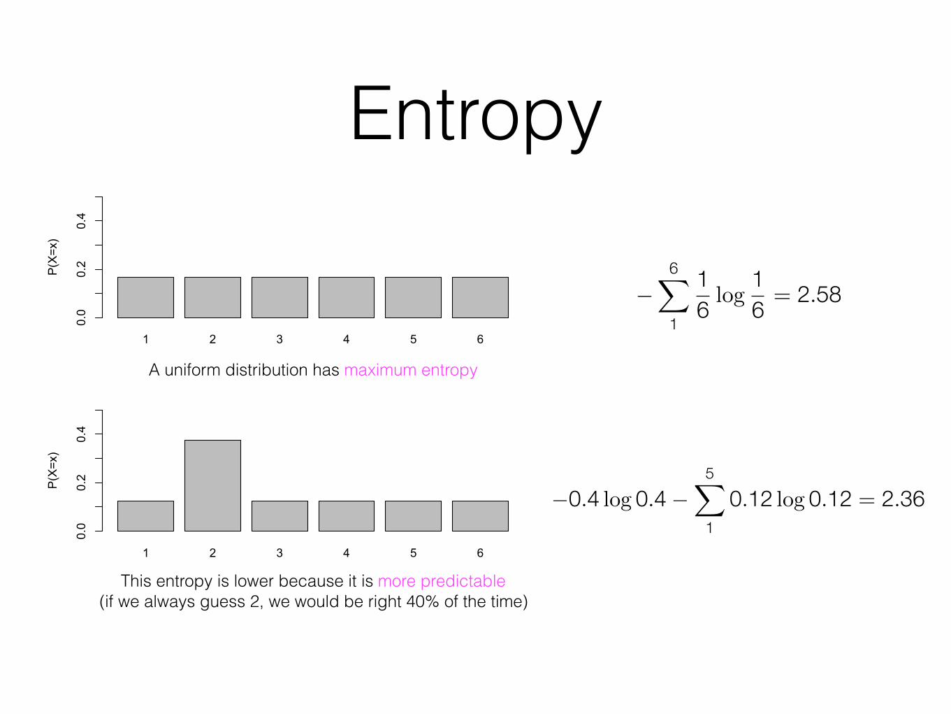
Entropy

• a great _______

• the oakland ______

��

x�XP(x) logP(x)

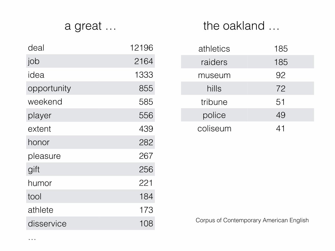
deal 12196job 2164idea 1333opportunity 855weekend 585player 556extent 439honor 282pleasure 267gift 256humor 221tool 184athlete 173disservice 108…

Corpus of Contemporary American English

a great …

athletics 185raiders 185

museum 92hills 72

tribune 51police 49

coliseum 41

the oakland …

Entropy

• High entropy means the phenomenon is less predictable

• Entropy of 0 means it is entirely predictable.

��

x�XP(x) logP(x)

Entropy

1 2 3 4 5 6

P(X=x)

0.0

0.2

0.4

1 2 3 4 5 6

P(X=x)

0.0

0.2

0.4

A uniform distribution has maximum entropy

This entropy is lower because it is more predictable (if we always guess 2, we would be right 40% of the time)

�6�

1

16 log

16 = 2.58

�0.4 log 0.4 �5�

10.12 log 0.12 = 2.36

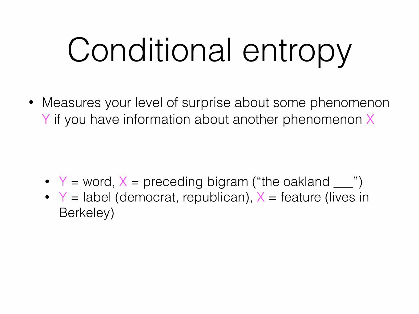
Conditional entropy• Measures your level of surprise about some phenomenon

Y if you have information about another phenomenon X

• Y = word, X = preceding bigram (“the oakland ___”) • Y = label (democrat, republican), X = feature (lives in

Berkeley)

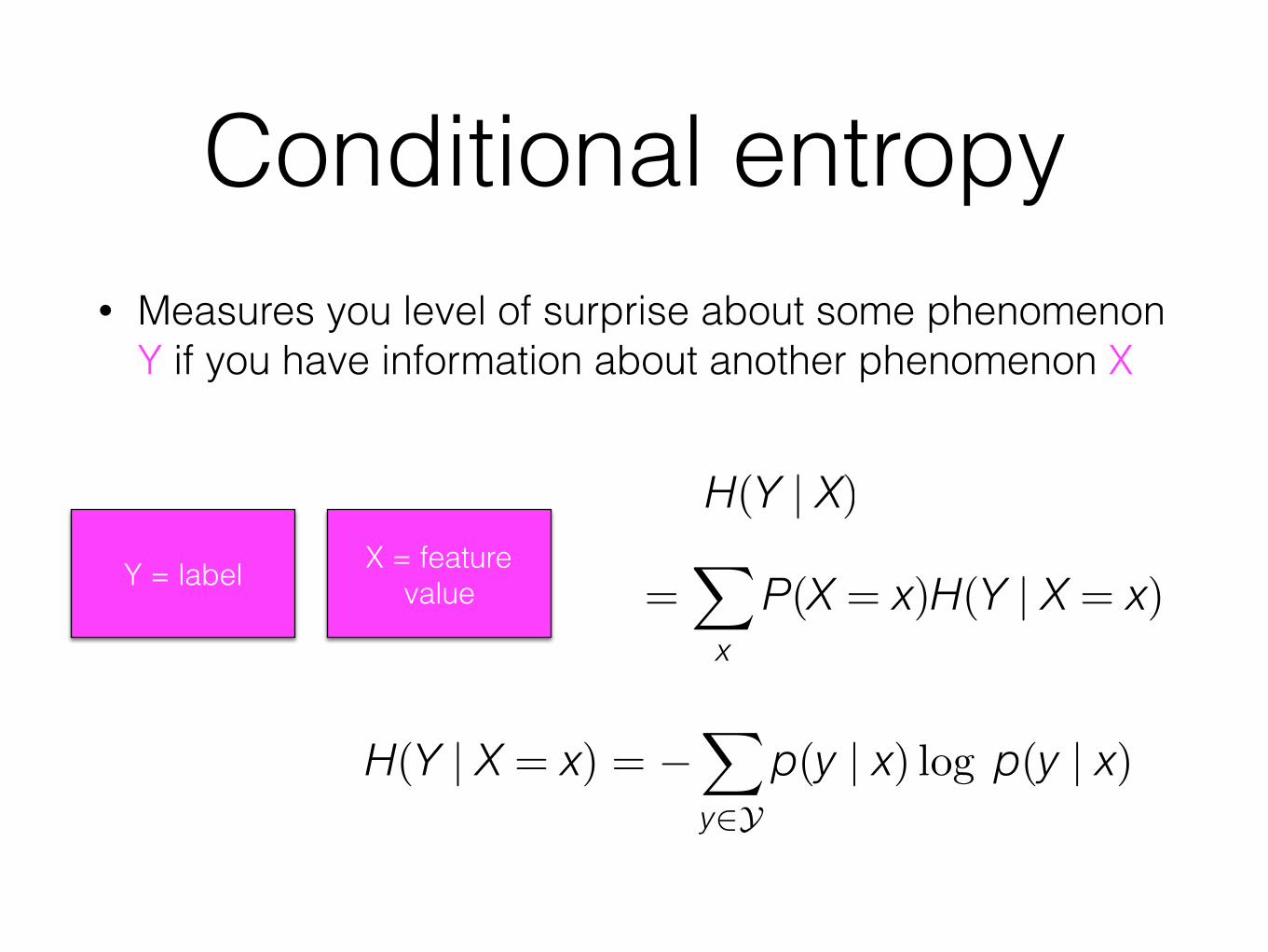
Conditional entropy• Measures you level of surprise about some phenomenon

Y if you have information about another phenomenon X

H(Y | X)

=�

xP(X = x)H(Y | X = x)

X = feature valueY = label

H(Y | X = x) = ��

y�Yp(y | x) log p(y | x)

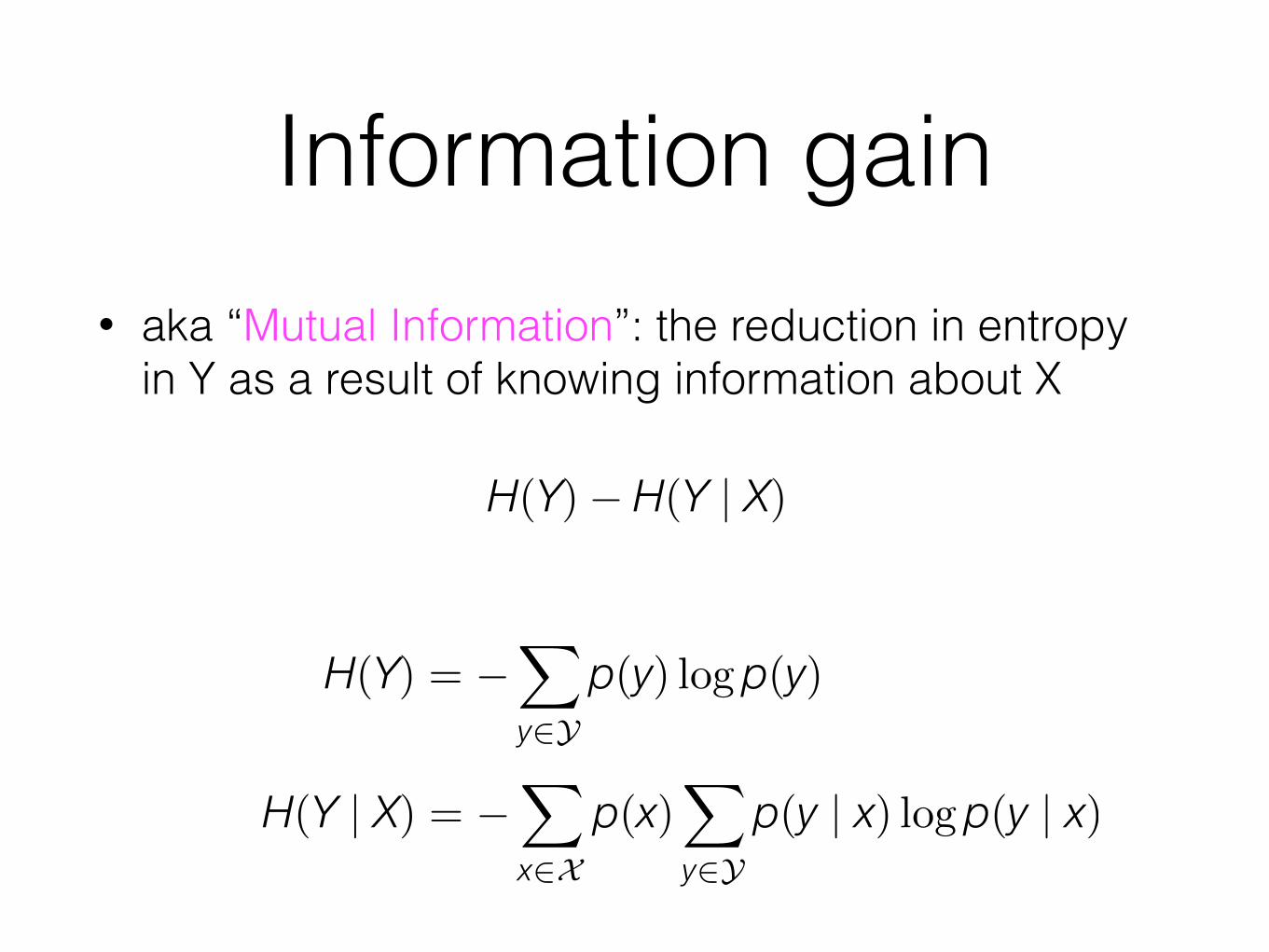
Information gain• aka “Mutual Information”: the reduction in entropy

in Y as a result of knowing information about X

H(Y) � H(Y | X)

H(Y) = ��

y�Yp(y) log p(y)

H(Y | X) = ��

x�Xp(x)

�

y�Yp(y | x) log p(y | x)

1 2 3 4 5 6

x1 0 1 1 0 0 1

x2 0 0 0 1 1 1

y ⊕ ⊖ ⊖ ⊕ ⊕ ⊖

Which of these features gives you more information about y?

1 2 3 4 5 6

x1 0 1 1 0 0 1

x2 0 0 0 1 1 1

y ⊕ ⊖ ⊖ ⊕ ⊕ ⊖

x ∈ 𝒳 0 1

y ∈ 𝒴 3⊕ 0⊖ 0⊕ 3⊖x1

x ∈ 𝒳 0 1

y ∈ 𝒴 3⊕ 0⊖ 0⊕ 3⊖

H(Y | X) = ��

x�Xp(x)

�

y�Yp(y | x) log p(y | x)

x1

P(y = + | x = 0) =3

3 + 0 = 1

P(y = � | x = 0) =0

3 + 0 = 0

P(y = � | x = 1) =3

3 + 0 = 1

P(y = + | x = 1) =0

3 + 0 = 0

P(x = 0) =3

3 + 3 = 0.5

P(x = 1) =3

3 + 3 = 0.5

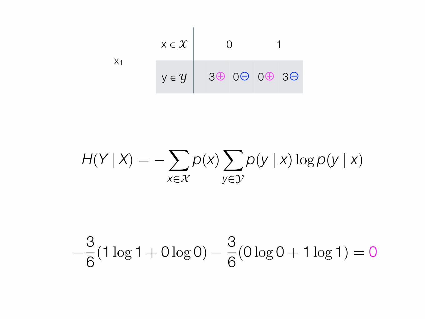
H(Y | X) = ��

x�Xp(x)

�

y�Yp(y | x) log p(y | x)

x ∈ 𝒳 0 1

y ∈ 𝒴 3⊕ 0⊖ 0⊕ 3⊖x1

�36 (1 log 1 + 0 log 0) � 3

6 (0 log 0 + 1 log 1) = 0

1 2 3 4 5 6

x1 0 1 1 0 0 1

x2 0 0 0 1 1 1

y ⊕ ⊖ ⊖ ⊕ ⊕ ⊖

x ∈ 𝒳 0 1

y ∈ 𝒴 1⊕ 2⊖ 2⊕ 1⊖x2

x ∈ 𝒳 0 1

y ∈ 𝒴 1⊕ 2⊖ 2⊕ 1⊖x2

P(y = + | x = 0) =1

1 + 2 = 0.33

P(y = � | x = 0) =2

1 + 2 = 0.67

P(y = � | x = 1) =1

1 + 2 = 0.33

P(y = + | x = 1) =2

1 + 2 = 0.67

P(x = 0) =3

3 + 3 = 0.5

P(x = 1) =3

3 + 3 = 0.5

H(Y | X) = ��

x�Xp(x)

�

y�Yp(y | x) log p(y | x)

x ∈ 𝒳 0 1

y ∈ 𝒴 1⊕ 2⊖ 2⊕ 1⊖x2

�36 (0.33 log 0.33 + 0.67 log 0.67) � 3

6 (0.67 log 0.67 + 0.33 log 0.33) = 0.91

Feature H(Y | X)

follow clinton 0.91

follow trump 0.77

“benghazi” 0.45

negative sentiment + “benghazi” 0.33

“illegal immigrants” 0

“republican” in profile 0.31

“democrat” in profile 0.67

self-reported location = Berkeley 0.80

In decision trees, the feature with the lowest conditional entropy/highest information gain defines the “best split”

MI = IG = H(Y) � H(Y | X)

for a given partition, H(Y) is the same for all features, so we can ignore it when deciding

among them

Feature H(Y | X)

follow clinton 0.91

follow trump 0.77

“benghazi” 0.45

negative sentiment + “benghazi” 0.33

“illegal immigrants” 0

“republican” in profile 0.31

“democrat” in profile 0.67

self-reported location = Berkeley 0.80

How could we use this in other models (e.g., the perceptron)?

Decision trees

BestSplit identifies the feature with the highest information gain and partitions the data according to values for that feature

Gini impurity• Measure the “purity” of a partition (how diverse the labels

are). If we were to pick an element in D and assign a label in proportion to the label distribution in D, how often would we make a mistake?

�

y�Ypy(1 � py)

Probability of selecting an item with label y at random

The probability of randomly assigning it the wrong label

Gini impurity

x ∈ 𝒳 0 1

y ∈ 𝒴 3⊕ 0⊖ 0⊕ 3⊖x1

�

y�Ypy(1 � py)

G(x1) = (3

3 + 3 )0 + (3

3 + 3 )0 = 0

x ∈ 𝒳 0 1

y ∈ 𝒴 1⊕ 2⊖ 2⊕ 1⊖x2

G(0) = 0.33 � (1 � 0.33) + 0.67 � (1 � 0.67) = 0.44

G(1) = 0.67 � (1 � 0.67) + 0.33 � (1 � 0.33) = 0.44

G(x2) = (3

3 + 3 )0.44 + (3

3 + 3 )0.44 = 0.44

G(0) = 1 � (1 � 1) + 0 � (1 � 0) = 0

G(0) = 0 � (1 � 0) + 1 � (1 � 1) = 0

Classification

𝓧 = set of all skyscrapers 𝒴 = {art deco, neo-gothic, modern}

A mapping h from input data x (drawn from instance space 𝓧) to a label (or labels) y from some enumerable output space 𝒴

x = the empire state building y = art deco

lives in Berkeley

follows Trump

contains “email”

profile contains

“Republican”

follows Trump

RD

RD

RD

yes

yes

yes

no

no

no

no

no yes

yes

Feature Value

follow clinton 0

follow trump 0

“benghazi” 0

negative sentiment + “benghazi” 0

“illegal immigrants” 0

“republican” in profile 0

“democrat” in profile 0

self-reported location = Berkeley 1 The tree that we’ve learned is the mapping ĥ(x)

lives in Berkeley

follows Trump

contains “email”

profile contains

“Republican”

follows Trump

RD

RD

RD

yes

yes

yes

no

no

no

no

no yes

yes

Feature Value

follow clinton 0

follow trump 0

“benghazi” 0

negative sentiment + “benghazi” 0

“illegal immigrants” 0

“republican” in profile 0

“democrat” in profile 0

self-reported location = Berkeley 1

How is this different from the perceptron?

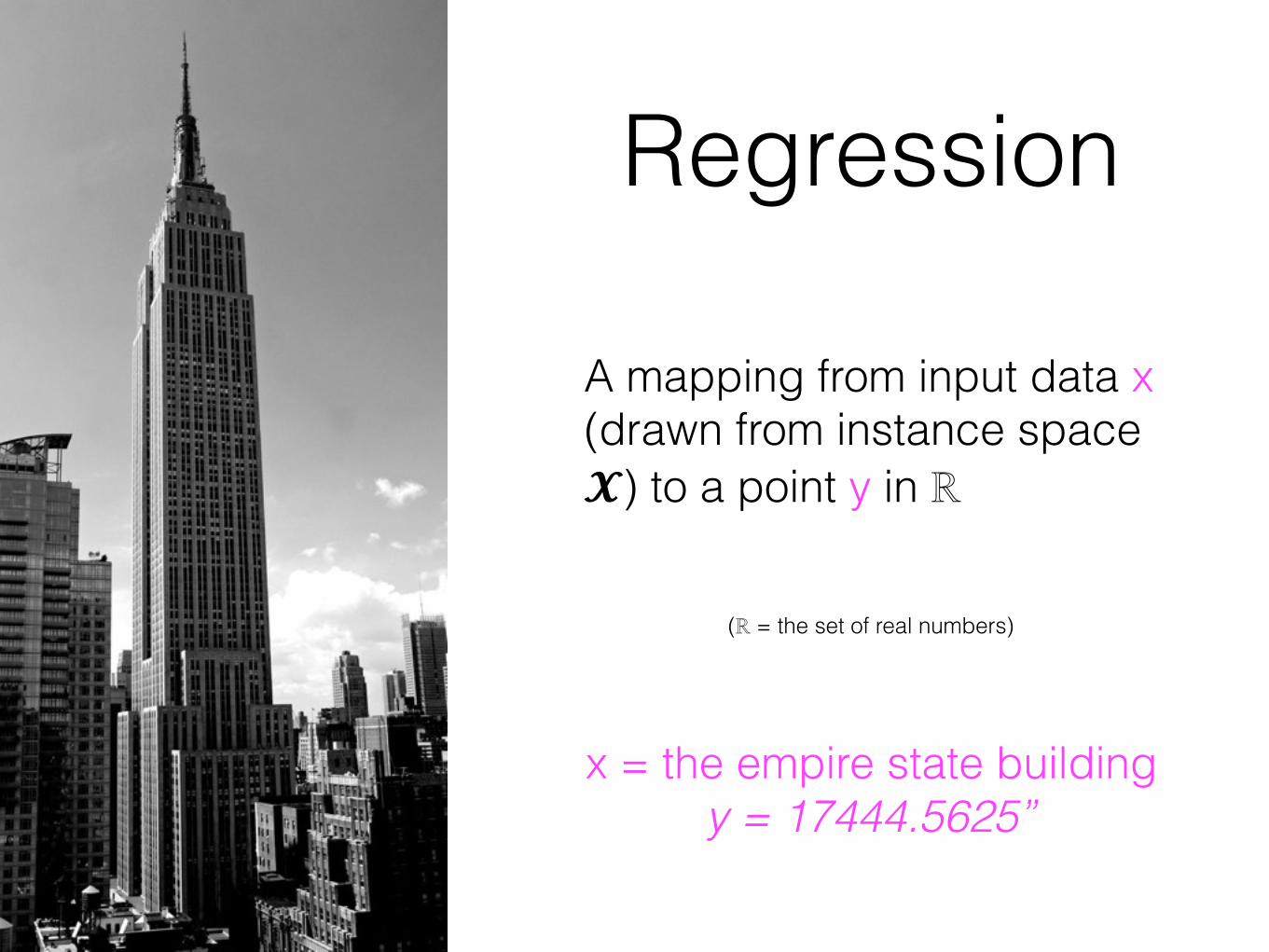
Regression

x = the empire state building y = 17444.5625”

A mapping from input data x (drawn from instance space 𝓧) to a point y in ℝ

(ℝ = the set of real numbers)

Feature Value

follow clinton 0

follow trump 0

“benghazi” 0

negative sentiment + “benghazi” 0

“illegal immigrants” 0

“republican” in profile 0

“democrat” in profile 0

self-reported location = Berkeley 1

lives in Berkeley

follows Trump

contains “email”

profile contains

“Republican”

follows Trump

$1$7

$2$13

$0$10

yes

yes

yes

no

no

no

no

no yes

yes

Decision trees

from Flach 2014

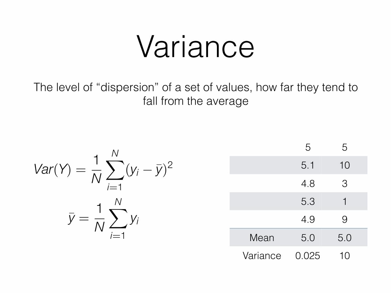
VarianceThe level of “dispersion” of a set of values, how far they tend to

fall from the average

5 5

5.1 10

4.8 3

5.3 1

4.9 9

Mean 5.0 5.0

Variance 0.025 10

0 2 4 6 8 10

0 2 4 6 8 10

VarianceThe level of “dispersion” of a set of values, how far they tend to

fall from the average

5 5

5.1 10

4.8 3

5.3 1

4.9 9

Mean 5.0 5.0

Variance 0.025 10

y =1N

N�

i=1yi

Var(Y) =1N

N�

i=1(yi � y)2

Regression trees• Rather than using entropy/Gini as a splitting

criterion, we’ll find the feature that results in the lowest variance of the data after splitting on the feature values.

1 2 3 4 5 6

x1 0 1 1 0 0 1

x2 0 0 0 1 1 1

y 5.0 1.7 0 10 8 2.2

x ∈ 𝒳 0 1

y ∈ 𝒴 5.0, 10, 8 1.7, 0, 2.2

Var 6.33 1.33

x1

366.33 +

361.33 = 3.83Average Variance:

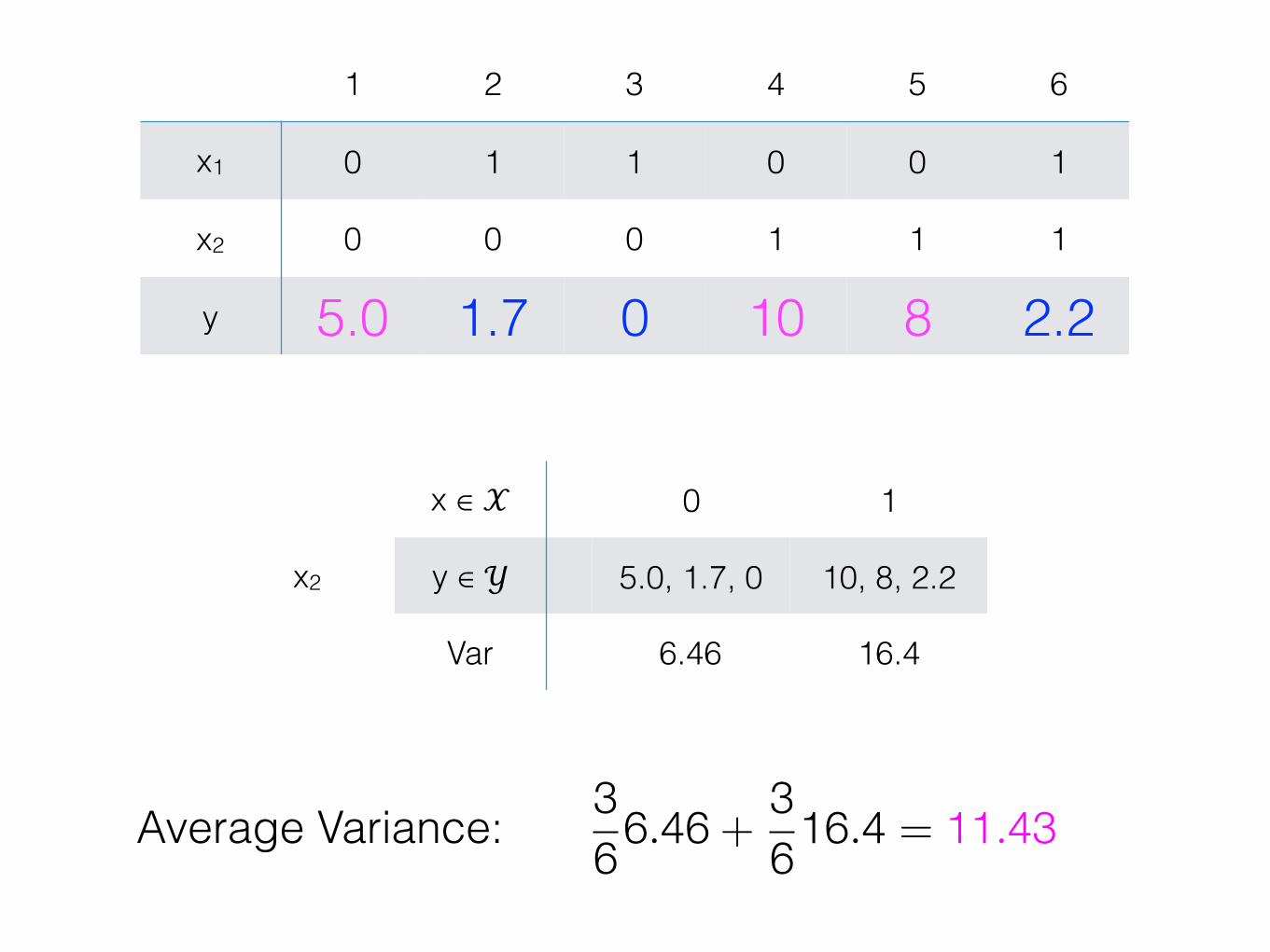
1 2 3 4 5 6

x1 0 1 1 0 0 1

x2 0 0 0 1 1 1

y 5.0 1.7 0 10 8 2.2

x ∈ 𝒳 0 1

y ∈ 𝒴 5.0, 1.7, 0 10, 8, 2.2

Var 6.46 16.4

x2

Average Variance: 366.46 +

3616.4 = 11.43

Regression trees• Rather than using entropy/Gini as a splitting

criterion, we’ll find the feature that results in the lowest variance of the data after splitting on the feature values.

• Homogeneous(D): the elements in D are homogeneous enough that they can be labeled with a single label. Variance < small threshold.

• Label(D): the single most appropriate label for all elements in D; the average value of y among D

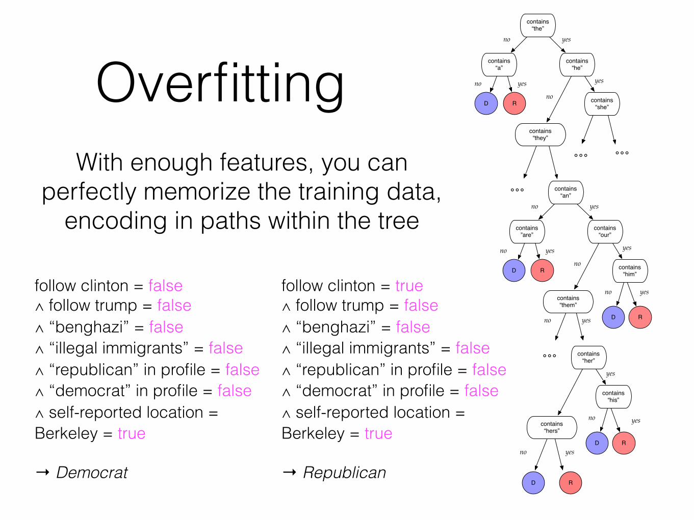
Overfitting…

contains “the”

contains “a”

contains “he”

contains “they”

contains “she”RD

yes

yes

no

no

no yes

contains “an”

contains”are”

contains “our”

contains “them”

contains “him”

RD

RD

yes

yes

yes

no

no

no

no

no yes

yes

…

…

contains “her”

contains “hers”

contains “his”

R

RD

yes

no

yes

…

D

no

yes

With enough features, you can perfectly memorize the training data,

encoding in paths within the tree

follow clinton = false ∧ follow trump = false ∧ “benghazi” = false ∧ “illegal immigrants” = false ∧ “republican” in profile = false ∧ “democrat” in profile = false ∧ self-reported location = Berkeley = true

→ Democrat

follow clinton = true ∧ follow trump = false ∧ “benghazi” = false ∧ “illegal immigrants” = false ∧ “republican” in profile = false ∧ “democrat” in profile = false ∧ self-reported location = Berkeley = true

→ Republican

Pruning

• One way to prevent overfitting is to grow the tree to an arbitrary depth, and then prune back layers (delete subtrees)

…

contains “the”

contains “a”

contains “he”

contains “they”

contains “she”RD

yes

yes

no

no

no yes

contains “an”

contains”are”

contains “our”

contains “them”

contains “him”

RD

RD

yes

yes

yes

no

no

no

no

no yes

yes

…

…

contains “her”

contains “hers”

contains “his”

R

RD

yes

no

yes

…

D

no

yes

Pruning

• Deeper into the tree = more conjunctions of features; a shallower tree contains only the most important (by IG) features

Interpretability• Decision trees are considered a relatively

“interpretable” model, since they can be post-processed in a sequence of decisions

• If self-reported location = Berkeley and “benghazi” = false, then y = Democrat

• Manageable for trees of small depth, but not deep trees (each layer = one additional rule)

• Even in small trees, potentially many disjunctions (or for each terminal node)

Interpretability…

contains “the”

contains “a”

contains “he”

contains “they”

contains “she”RD

yes

yes

no

no

no yes

contains “an”

contains”are”

contains “our”

contains “them”

contains “him”

RD

RD

yes

yes

yes

no

no

no

no

no yes

yes

…

…

contains “her”

contains “hers”

contains “his”

R

RD

yes

no

yes

…

D

no

yes

• Low bias: decision trees can perfectly match the training data (learning a perfect path through the conjunctions of features to recover the true y.

• High variance: because of that, they’re very sensitive to whatever data you train on, resulting in very different models on different data

Solution: train many models

• Bootstrap aggregating (bagging) is a method for reducing the variance of a model by averaging the results from multiple models trained on slightly different data.

• Bagging creates multiple versions of your dataset using the bootstrap (sampling data uniformly and with replacement)

Bootstrapped dataoriginal x1 x2 x3 x4 x5 x6 x7 x8 x9 x10

rep 1 x3 x9 x1 x3 x10 x6 x2 x9 x8 x1

rep 2 x7 x9 x1 x1 x4 x9 x10 x7 x5 x6

rep 3 x2 x3 x5 x8 x9 x8 x10 x1 x2 x4

rep 4 x5 x1 x10 x5 x4 x2 x1 x9 x8 x10

Train one decision tree on each replicant and average the predictions (or take the majority vote)

De-correlating further

• Bagging is great, but the variance goes down when the datasets are independent of each other. If there’s one strong feature that’s a great predictor, then the predictions will be dependent because they all have that feature

• Solution: for each trained decision tree, only use a random subset of features.

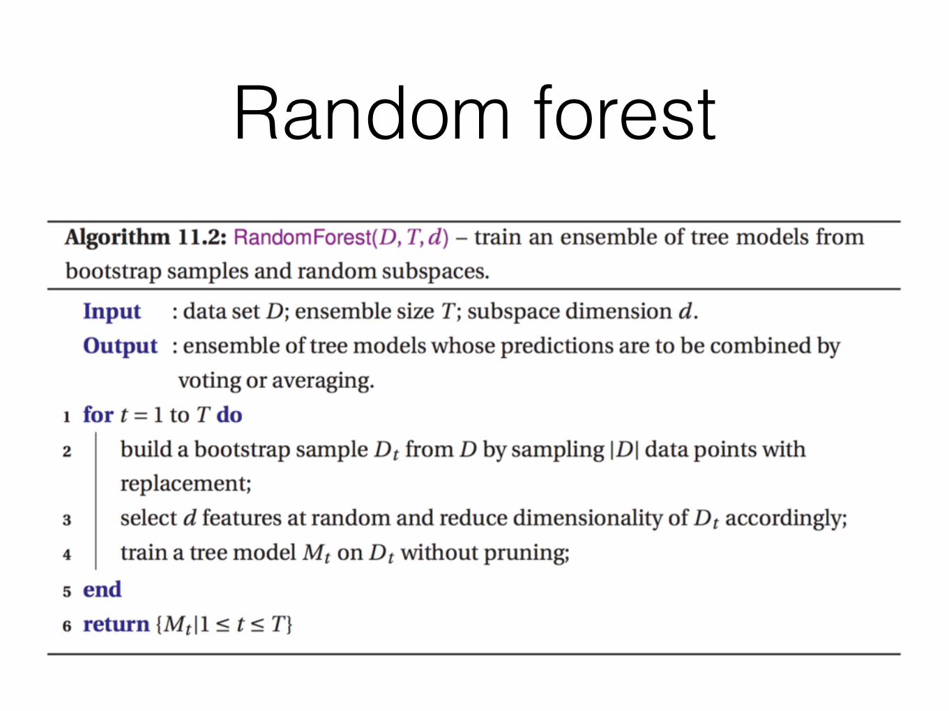
Random forest

Krippendorff (2004)

Project proposal, due 2/19• Collaborative project (involving 2 or 3 students), where the

methods learned in class will be used to draw inferences about the world and critically assess the quality of those results.

• Proposal (2 pages):

• outline the work you’re going to undertake • formulate a hypothesis to be examined • motivate its rationale as an interesting question worth asking • assess its potential to contribute new knowledge by

situating it within related literature in the scientific community. (cite 5 relevant sources)

• who is the team and what are each of your responsibilities (everyone gets the same grade)