-0-

Decomposition of Labor Productivity Growth: A

Multilateral Production Frontier Approach

Konstantinos Chatzimichael and Vangelis Tzouvelekas

(Dept. of Economics, University of Crete, GREECE)

ABSTRACT

This paper develops a parametric decomposition framework of labor productivity growth

relaxing the assumption of labor-specific efficiency. The decomposition analysis is

applied to a sample of 52 developed and developing countries from 1965-90. A

generalized Cobb-Douglas functional specification is used taking into account differences

in technological structures across group of countries to approximate aggregate production

technology using Jorgenson and Nishimizu (1978) bilateral model of production.

Measurement of labor efficiency is based on Kopp’s (1981) orthogonal non-radial index

of factor-specific efficiency modified in a parametric frontier framework. The empirical

results indicate that the weighted average annual rate of labor productivity growth was

1.43 per cent over the period analyzed. Technical change was found to be the driving

force of labor productivity, while improvements in labor efficiency and human capital

account approximately for the 22 per cent of that productivity growth.

Keywords: labor efficiency and productivity growth, multilateral production frontier.

JEL Classification: J24, O40, C23

-1-

DECOMPOSITION OF LABOR PRODUCTIVITY GROWTH: A

MULTILATERAL PRODUCTION FRONTIER APPROACH

INTRODUCTION

The productivity fall observed in many developed and developing countries during the

60’s and early 70’s triggered an intense public debate aimed to unravel the internal

mechanism of productivity growth. This heated debate had resulted to an enormous

theoretical and empirical literature directed to the investigation of the proximate causes of

the observed differences in per-capita income across developing and developed countries.

Most researchers used the cross-sectional version of the familiar growth accounting

framework of Solow (1957) to decompose country variations in the levels of output per

worker into parts attributed to the variation in the factors of production and productivity

growth. The results lead to the conclusion that the residual productivity rather than factor

accumulation accounts for most of the income and growth differences across nations (see

Caselli (2005) and the references cited therein). This finding although it uncovers the

proximate causes of income differentials is unsatisfactory in the sense that the ultimate

causes that lead to different levels of productivity are not explained. If we accept that

productivity differences are large, then we are left with a shortage of convincing

explanation for this result. The later is important as different sources of productivity

differentials require different policy measures to enhance economic growth either in

developed or developing nations (Prescott, 1988).

Since much of these productivity variations represents differences in technological

structures, then there should be an adequate explanation why non-rival innovations do not

-2-

diffuse across borders. And if they do, then why we still observe differences in measured

productivity rates. If there is a uniform worldwide production frontier, then all of the

observed differences in productivity reflect a gap from this frontier. Obviously there are

strong barriers to adoption across countries related to the institutional and cultural

environment preventing many countries from using that common technological structure.

Olson (1982) and Krusell and Rios-Rull (1996) argue, that vested interest groups are

lobbying for market power, protection from competition, limiting factor mobility and

then blocking adoption of rival technologies through a political process. Parente and

Prescott (1999) provide a theoretical model where the existence of monopoly power

extend beyond the traditional deadweight loss affecting the adoption of new technologies

as well as the appropriate use of technologies already adopted.

Relative recently economic growth literature questions the above perspective,

recognizing that the technology frontier is not uniform. In other words, it admits that not

every country face the same technological conditions. According to this perception

countries choose the best production technologies available to them given their internal

economic and structural conditions. Obviously factor endowments as well as the

institutional and cultural environment affect these choices as some technologies may be

less productive than others. For instance, ICT technologies enhance social welfare

through structural transformation in production networks and social customs but at the

same time require human capital, i.e., high literacy rates, to function properly. Basu and

Weil (1998) and Acemoglou and Zilibotti (2001), explored the appropriateness of

technology paradigm to explain differences in income levels and economic convergence.

They both conclude that developed countries invent new technologies that are compatible

-3-

with their own resource endowments and these technologies do not work appropriately in

developing countries with a different input mix. This implies that the adoption of a

modern technology by poor countries do not raise their productivity levels as it is

inappropriate to them. So the assumption of the same technological structure may not be

adequate to explain productivity variations and empirical work should take that into

account.

Under both paradigms, one would expect all countries to operate on their own or to

the common technological frontier being thus fully efficient. Empirical evidence though

suggest that rather the opposite is true. Several authors suggest that rarely countries are

exploring fully the potential of the existing technology operating far from their respective

production frontier (e.g., Färe et al., 1994; Kumar and Russell, 2002; Los and Timmer,

2005; Badunenko et al., 2008). Theoretical models of explaining inefficiency in resource

utilization, focus on the role of institutions and social structures to explain why the

common or country-specific production technology is not utilized appropriately by

individual countries. Apart of the availability of the technology, other factors must be

present such as strong investment, a well trained work force, R&D activity, trading

relationships, a receptive political structure that Abramovitz (1986) summarizes under the

term social capability. However, all these elements of efficiency determination are not

affecting the efficient use of all inputs in the same manner. For instance, lack of working

experience affects rather more intensively labor efficiency than capital utilization.

Nevertheless empirical studies, besides analyzing labor productivity differentials, they

utilize an aggregate output or input inefficiency index. Important information, valuable

-4-

from a policy perspective, can be gained by providing an empirical analysis focusing

exclusively on labor-specific efficiency.

Probably the most important aspect related with resource utilization and therefore

productivity differentials across countries, recognized by many researcher, is the role of

human capital. Inspired by the early approaches on human capital theory (Schultz, 1961;

Becker, 1975), many empirical researchers have focused on the important role played by

educational levels in the efficiency of input utilization and hence on the growth process.

In these early theoretical contributions schooling is viewed as an investment in skills

having a direct effect on labor productivity as well as an indirect one through the

improvement of worker’s ability to work efficiently (Welch, 1970). Griliches (1970) and

Jorgenson and Fraumeni (1993) found that a significant portion of differentials is

attributed directly to increases in educational levels. On the other hand, Welch (1970)

and Bartel and Lichtenberg (1987), among others, found that highly educated workers

have a comparative advantage with regard to the implementation of new technologies

exhibiting therefore higher efficiency levels. Recently the development of detailed

educational data by Barro and Lee (1993; 2001) and the formulation of endogenous

growth models by Lucas (1988) and Romer (1990), enabled the empirical analysis on the

role of education in economic growth. All of these studies on growth accounting again

indicated that a significant portion of measured productivity growth is attributed directly

to increases in educational levels of the labor force (e.g., Benhabib and Spiegel, 1994;

O’Neil, 1995; Bils and Klenow, 2000). Regardless of the nature and the aims of these

studies, they provided unshaken evidence about the important role played by human

-5-

capital in the growth process, suggesting that it is an important element of any

productivity decomposition analysis and it should be included in any empirical research.

Motivated by the works of Färe et al., (1994), Kumar and Russell (2002) and

Henderson and Russell (2005), we attempt in this paper to contribute in the relevant

literature providing a theoretically consistent parametric decomposition of labor

productivity growth. According to these studies labor productivity is decomposed into

the rates of growth of factor intensities and TFP. However, shifts in relative capital-labor

prices and the biases of technological change are also important possibilities for changes

in the growth rate of factor intensities. Taking that into account, our decomposition

framework provides a more detailed analysis of changes in labor productivity across

countries. First, we focus on labor-specific inefficiency rather than an output efficiency

measure which is more relevant when labor productivity growth is analyzed. The

proposed index for measuring labor-specific technical and allocative efficiency is based

on Kopp’s (1981) orthogonal non-radial index of technical efficiency modified in a

parametric frontier framework. Then the derived index of labor-specific efficiency is

used to provide a complete decomposition framework of labor productivity growth.

Second, we dispense with the assumption of a common worldwide production

technology in estimated parametrically the aggregate production frontier. Our empirical

aggregate production frontier model is based on the generalized Cobb-Douglas functional

specification suggested by Fan (1991) that accounts for biases in technical change,

extended into a multilateral context in order to take into account differences in

technological structures among countries in the sample using Jorgenson and Nishimizu

(1978) bilateral production structure. In that way formal statistical testing can be used to

-6-

examine the existence of a common worldwide technology utilized by all countries in the

sample. The production frontier was estimated econometrically, incorporating human

capital, using Cornwell et al., (1990) fixed effects formulation that allows for country

specific time varying inefficiencies. Following Griliches (1963), human capital is

introduced as an augmenting factor of labor input using Hall and Jones (1999)

construction, enabling thus the identification of both its direct and indirect role on

measured labor productivity.

Using this general framework we provide a complete decomposition analysis of

labor productivity growth in a sample of 52 developed and developing countries from

1965-90 drawn from Penn World Tables. Besides decomposing the growth of output per

worker into technological change, technological catch-up and physical and human capital

accumulation, our decomposition analysis accounts for the existence of variable returns

to scale and for the labor biases of technical change due to changes in relative factor

prices. The remaining paper is organized as follows. In the next section, we present the

theoretical framework for measuring labor productivity growth in a parametric context.

Next section 3 presents data description and describes the empirical model and estimation

procedures. Section 4 discusses the empirical results while, the last section concludes the

paper.

THEORETICAL FRAMEWORK

Let assume that countries in period t utilize labor, physical and human capital to produce

a single aggregate output y +∈ℜ through a well-behaved technology described by the

following non-empty, closed set:

-7-

( ) ( ){ }tT k ,l , , y y f k ,l , ,tε ε= ≤: (1)

where k +∈ℜ denotes physical capital, l +∈ℜ labor, ε +∈ℜ human capital, t +∈ℜ is a

time index, and, ( ) 4f k ,l , ,t :ε + +ℜ →ℜ is a strictly increasing, differentiable concave

production function, representing the maximal output from physical capital and labor use

given human capital and technological constraints. Using (1) we can define the input

correspondence set as all the input combinations capable of producing y +∈ℜ as:

( ) ( ) ( ){ }3 : tL y k ,l , k ,l , , y Tε ε+= ∈ℜ ∈ . Given the assumptions made on ( )f i , the input

correspondence set is a closed convex set satisfying strong disposability of labor and

physical capital inputs.

Alternatively, aggregate production technology may be defined by the dual cost

function ( ) ( ) 3 1, , , :C y t yε ++ ++×ℜ →ℜw R as:

( ) ( ){ }:l kk ,lC , y, ,t min w l w k y f k ,l , ,tε ε= + ≤w (2)

where ( ) ( ){ }:R y y L y+= ∈ℜ ≠ ∅ , { } 2l kw ,w ++= ∈ℜw are the strictly positive effective

labor and capital prices. The cost function is differentiable in all its arguments, non-

decreasing in w and y, non-increasing in ε and t, and homogeneous of degree one in w.

At this point we may assume that the production of aggregate output may not be

technical efficient, i.e., countries are not able to minimize input use in the production of a

given aggregate output in the light of the prevailing factor prices. Concentrating in labor

-8-

input it should hold that ( )ly f k , l , ,tθ ε= ⋅ where θ l is a measure of labor-specific

technical efficiency indicating how much labor should be reduced still being able to

produce the same level of aggregate output. Formally, θ l may be defined according to

Kopp’s (1981) orthogonal non-radial index of input-specific technical efficiency:1

( ){ }: 0l

KP l l lLTE min , y f k, l , ,tθ

θ θ θ ε= > ≤ ⋅ (3)

which is bounded between zero and one, i.e., 0 < LTE KP ≤ 1. Graphically, the above

definition is presented in Figure 1. Assuming that country i operates at point A in the

graph utilizing 0l quantity from labor and 0k quantity from capital producing y level of

aggregate output. Obviously the country in question is technically inefficient as it is

possible to reduce input use moving on the respective isoquant and still being able to

produce the same level of aggregate output. If inefficiency arises only from labor use

then an obvious change would be the movement to point B on the graph, where capital

use remains unchanged but labor quantity has been reduced to 1 0ll lθ= .

However, still at point B country is not fully efficient. Although labor use is at its

technical efficient point country fails to utilize an appropriate capital-labor mix given the

input prices it faces. This is achieved at point C where cost of aggregate production is

minimized given factor prices, human capital endowments and production technology. A

measure of the extent for this allocation error is provided by the following ratio:

( )*

l

l , y, ,tLAE

lε

θ=

w (4)

-9-

where ( )*l , y, ,tεw is the Hicksian constant output demand function for labor obtained

from (2) through Shephard’s lemma which is non-decreasing in y and kw and non-

increasing in lw , ε and t. The above ratio may be viewed as an index of labor allocative

efficiency which, contrary to its technical efficiency index, can take positive values

below or above unity and it is equal to one when ( )wl *l l , y, ,tθ ε= . If it is greater (less)

than one, labor is under- (over-) utilized at its technically efficient level given capital and

labor prices. In developed countries that are abundant in capital input, labor allocative

efficiency is expected to be greater than one whereas in developing countries that are

abundant in labor input less than one assuming competitive factor prices.

Using (3) and (4) we may define overall labor efficiency by the product of labor

technical and allocative efficiency or, equivalently, by the ratio of optimal to observed

labor use as:

( ) ( )* *lKP

l

l , y, ,t l , y, ,tlLOE LTE LAEl l l

ε εθθ

= × = × =w w

(5)

which is equal to one when ( )w*l l , y, ,tε= . When LOE > 1, individual country over-

utilizes labor input at the observed point given the prevailing factor prices, whereas when

LOE < 1 labor is under-utilized.

Taking the logarithms on the last equality of (5) and totally differentiating with

respect to time we get:

-10-

( ) ( ) ( )

( ) ( )

*d dll l lk k

*dl

lnl , y, ,tLOE y e ,y, ,t w e ,y, ,t w

ln ylnl , y, ,t

e , y, ,t ltε

εε ε

εε ε

∂= + +

∂

∂+ + −

∂

ww w

ww

i i i i

i i (6)

where a dot over a function or a variable indicates its time rate of change,

( ) ( )*dll

l

lnl , y, ,te , y, ,t

ln wε

ε∂

=∂

ww and ( ) ( )*

dlk

k

lnl , y, ,te , y, ,t

ln wε

ε∂

=∂

ww are the compensated

own- and cross-price elasticities of labor demand, respectively and, ( )dle , y, ,tε ε =w

( )*lnl , y, ,tln

εε

∂∂

w is the compensated labor demand elasticity with respect to human

capital. Then, using the conventional divisia index of labor productivity, i.e.,

( )d ln y lLP y l

dt

i i i= = − , the time rate of change of the first equality in (5), i.e.,

KPLOE LTE LAE= +ii i

, and substituting them into (6), we obtain

( ) ( )

( ) ( ) ( )

1*

KP dll l

*d dlk k l

lnl , y, ,tLP LTE LAE y e ,y, ,t w

ln y

lnl , y, ,t e , y, ,t w e , y, ,t

tε

εε

εε ε ε

⎡ ⎤∂= + + − −⎢ ⎥∂⎣ ⎦

∂− − −

∂

ww

ww w

ii i i i

i i (7)

decomposing, thus, labor productivity growth into a labor-specific technical and

allocative inefficiency effect (first two terms), an output effect (third term), a substitution

effect (fourth and fifth terms), a human capital effect (sixth term) and, a technological

change effect (last term). Using the cost share equation of labor input, i.e.,

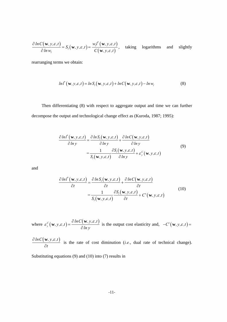
-11-

( ) ( )ll

lnC , y, ,tS , y, ,t

ln wε

ε∂

= =∂

ww ( )

( )

*lw l , y, ,tC , y, ,t

εε

ww

, taking logarithms and slightly

rearranging terms we obtain:

( ) ( ) ( )*l llnl , y, ,t ln S , y, ,t lnC ,y, ,t ln wε ε ε= + −w w w (8)

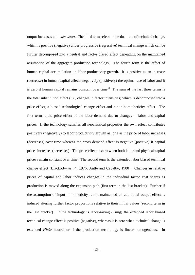
Then differentiating (8) with respect to aggregate output and time we can further

decompose the output and technological change effect as (Kuroda, 1987; 1995):

( ) ( ) ( )

( )( ) ( )1

*l

l Cy

l

lnl , y, ,t ln S , y, ,t lnC ,y, ,tln y ln y ln y

S ,y, ,t = , y, ,t

S , y, ,t ln y

ε ε ε

εε ε

ε

∂ ∂ ∂= +

∂ ∂ ∂

∂+

∂

w w w

ww

w

(9)

and

( ) ( ) ( )

( )( ) ( )1

*l

l t

l

lnl , y, ,t ln S , y, ,t lnC ,y, ,tt t t

S , y, ,t = C ,y, ,t

S , y, ,t t

ε ε ε

εε

ε

∂ ∂ ∂= +

∂ ∂ ∂∂

+∂

w w w

ww

w

(10)

where ( ) ( )Cy

lnC ,y, ,t, y, ,t

ln yε

ε ε∂

=∂

ww is the output cost elasticity and, ( )tC , y, ,tε− =w

( )lnC ,y, ,tt

ε∂∂w

is the rate of cost diminution (i.e., dual rate of technical change).

Substituting equations (9) and (10) into (7) results in

-12-

( ) ( ) ( )

( ) ( )

1KP C t dy l

Efficiency effect Technological Human capital effectScale effectchange effect

d dll l lk k

Price

LP LTE LAE , y, ,t y C , y, ,t e , y, ,t

e , y, ,t w e , y, ,t w

εε ε ε ε ε

ε ε

⎡ ⎤= + + − − −⎣ ⎦

− −

w w w

w w

ii i i i

i i

( )( ) ( )1 l l

leffectExtended labor biased techological change effect

S , y, ,t S , y, ,ty

S , y, ,t t ln yε ε

ε⎡ ⎤∂ ∂

− +⎢ ⎥∂ ∂⎣ ⎦

w ww

i (11)

which is the final decomposition formula of labor productivity growth. Specifically,

equation (11) attributes labor productivity growth into six sources. The first three terms

accounts for changes in TFP which in turn is decomposed into changes in labor

efficiency, the effect of scale economies and technological change. The first component

of the right hand side of (11) indicates changes in labor-specific technical and allocative

inefficiency over time. It is positive (negative) as labor technical and allocative

efficiency increases (decreases) over time.2 There is no a priori reason for both types of

efficiency to increase or decrease simultaneously (Schmidt and Lovell, 1980) nor that

their relative contribution should be of equal importance for productivity growth. More

importantly, what really matters in productivity growth decomposition analysis is not the

degree of efficiency itself, but its improvement over time. That is, even at low levels of

overall efficiency, output gains may be achieved by improving either technical or

allocative labor efficiency, or both. However, it seems difficult to achieve substantial

rates of growth at very high levels of technical and/or allocative efficiency. The second

term measures the relative contribution of scale economies to labor productivity growth.

Under constant returns-to-scale, i.e., ( ) 1Cy , y, ,tε ε =w , output growth or contraction

makes no contribution to labor productivity change and therefore this term vanishes. It is

positive (negative) under increasing (decreasing) returns-to-scale as long as aggregate

-13-

output increases and vice versa. The third term refers to the dual rate of technical change,

which is positive (negative) under progressive (regressive) technical change which can be

further decomposed into a neutral and factor biased effect depending on the maintained

assumption of the aggregate production technology. The fourth term is the effect of

human capital accumulation on labor productivity growth. It is positive as an increase

(decrease) in human capital affects negatively (positively) the optimal use of labor and it

is zero if human capital remains constant over time.3 The sum of the last three terms is

the total substitution effect (i.e., changes in factor intensities) which is decomposed into a

price effect, a biased technological change effect and a non-homotheticity effect. The

first term is the price effect of the labor demand due to changes in labor and capital

prices. If the technology satisfies all neoclassical properties the own effect contributes

positively (negatively) to labor productivity growth as long as the price of labor increases

(decreases) over time whereas the cross demand effect is negative (positive) if capital

prices increases (decreases). The price effect is zero when both labor and physical capital

prices remain constant over time. The second term is the extended labor biased technical

change effect (Blackorby et al., 1976; Antle and Capalbo, 1988). Changes in relative

prices of capital and labor induces changes in the individual factor cost shares as

production is moved along the expansion path (first term in the last bracket). Further if

the assumption of input homotheticity is not maintained an additional output effect is

induced altering further factor proportions relative to their initial values (second term in

the last bracket). If the technology is labor-saving (using) the extended labor biased

technical change effect is positive (negative), whereas it is zero when technical change is

extended Hicks neutral or if the production technology is linear homogeneous. In

-14-

homothetic technologies the second term of the extended labor biased technical change

effect vanishes as ( ) 0lS , y, ,tln y

ε∂=

∂w

.

DATA AND EMPIRICAL MODEL

For the quantitative measurement and decomposition of labor productivity growth we

utilized a balanced data set of 52 developed and developing countries covering the period

from 1965 to 1990.4 For aggregate output, physical capital and labor input we make use

of the Penn World Tables (ver. 5.6).5 For the calculation of capital and labor prices,

following the approach suggested by Mamuneas et al., (2006), we use the share of

employee compensation in national income published by the Total Economy Growth

Accounting Database of the Groningen Growth and Development Centre and National

Account Statistics of the United Nations (UN).6 Human capital was proxied using Barro

and Lee (1993; 2001) educational data that are available for the same group of countries

and for the same time period.7,8 Following Henderson and Russell (2005), we adopt Hall

and Jones (1999) construction where education appears as an augmentation factor for

labor using an exponential specification, i.e., ( ) ( )h eϕ εε = with ( )ϕ ε being a Mincerian

piecewise linear function with zero intercept and slope that varies according to the time

span.9 Following Psacharopoulos (1994) survey on the evaluation of the returns to

education, those parameters were defined as being 0.134 for the first four years, 0.101 for

the next four years and 0.068 for education beyond the eight year.

Our empirical model for providing measurement of labor productivity growth is

based on a Cobb-Douglas type of aggregate production frontier. Specifically, minimizing

-15-

the cost on the flexibility of the functional specification, we adopt a generalized Cobb-

Douglas (or quasi-translog) production frontier, proposed by Fan (1991). This functional

specification, although not enough flexible like the translog, it allows for variable returns

to scale, input-biased technical change, and time varying output and demand elasticities,

but it restricts the latter to be unchanged over countries. It permits statistical testing for

various features of the aggregate production technology, providing at the same time an

analytical closed form solution for the corresponding dual cost frontier necessary to

identify appropriately all terms in (11) (Fan and Pardey, 1997).

Since both developed and developing countries are included in the sample we

should take into account technological differences among them. To lessen these potential

biases in approximating production technology, we extent Jorgenson and Nishimizu

(1978) “bilateral” production structure into a “multilateral” context within the

generalized Cobb-Douglas production frontier model. Specifically, we distinguish six

different groups of countries (i.e., South and Central America, North America and

Oceana, Europe, Asia, Africa and Asian Tigers) assuming that each one of those groups

exhibit it’s “own” technological structure. In that way, on the one hand, it is possible to

identify differences in all terms appearing in (11) between group of countries that are

assumed to exhibit different technological conditions, while on the other, we allow for

more flexible patterns for technological features (i.e., returns to scale, technological

change, production and demand elasticities) between groups of countries lessened further

the cost of choosing a less flexible functional specification for the approximation of the

worldwide production technology.

-16-

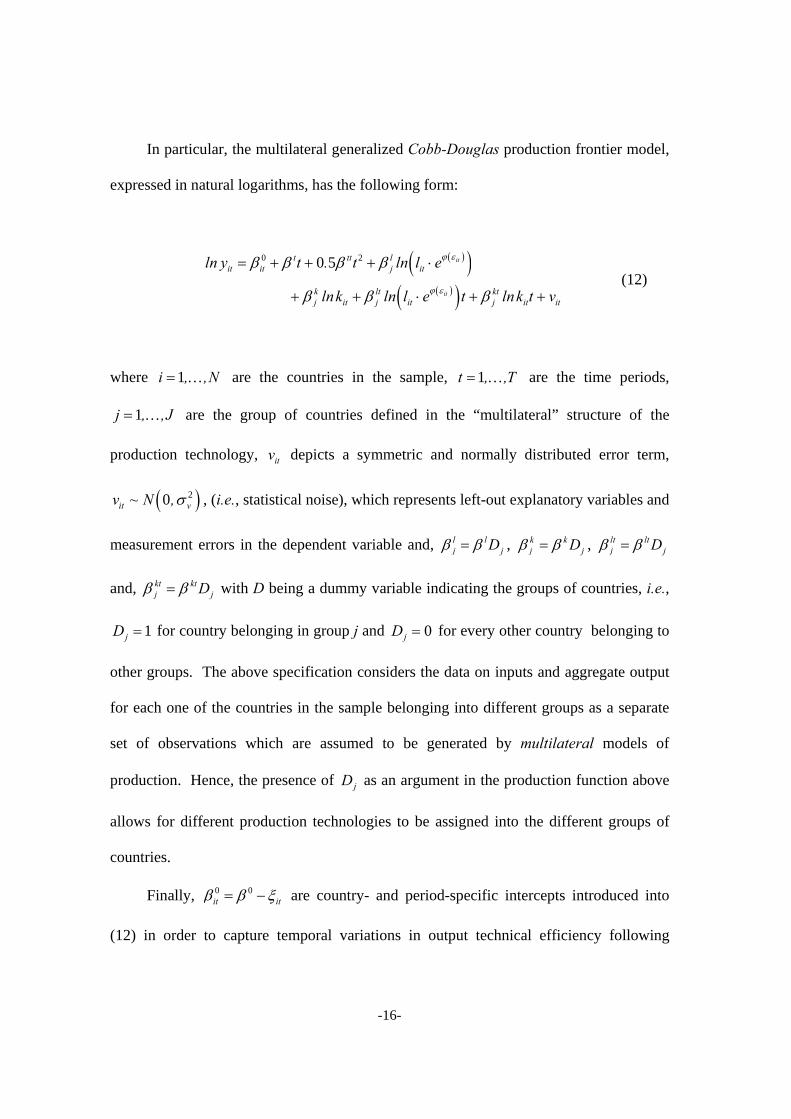
In particular, the multilateral generalized Cobb-Douglas production frontier model,

expressed in natural logarithms, has the following form:

( )( )

( )( )

0 20 5 it

it

t tt lit it j it

k lt ktj it j it j it it

ln y t . t ln l e

lnk ln l e t lnk t v

ϕ ε

ϕ ε

β β β β

β β β

= + + + ⋅

+ + ⋅ + + (12)

where 1i , ,N= … are the countries in the sample, 1t , ,T= … are the time periods,

1j , ,J= … are the group of countries defined in the “multilateral” structure of the

production technology, itv depicts a symmetric and normally distributed error term,

( )20it vv ~ N ,σ , (i.e., statistical noise), which represents left-out explanatory variables and

measurement errors in the dependent variable and, l lj jDβ β= , k k

j jDβ β= , lt ltj jDβ β=

and, kt ktj jDβ β= with D being a dummy variable indicating the groups of countries, i.e.,

1jD = for country belonging in group j and 0jD = for every other country belonging to

other groups. The above specification considers the data on inputs and aggregate output

for each one of the countries in the sample belonging into different groups as a separate

set of observations which are assumed to be generated by multilateral models of

production. Hence, the presence of jD as an argument in the production function above

allows for different production technologies to be assigned into the different groups of

countries.

Finally, 0 0it itβ β ξ= − are country- and period-specific intercepts introduced into

(12) in order to capture temporal variations in output technical efficiency following

-17-

Cornwell et al., (1990) fixed effects specification. According to this formulation output

technical inefficiency is assumed to follow a quadratic pattern over time, i.e.,

ξit = ζ i0 +ζ i1t +ζ i2t2 (13)

where, 0iζ , 1iζ and 2iζ are the ( )3N × unknown parameters to be estimated. If

1 2 0i iζ ζ= = i∀ , then output technical efficiency is time-invariant, while when 1 1iζ ζ=

and 2 2iζ ζ= i∀ then output technical efficiency is time-varying following, however, the

same pattern for all countries in the sample.10

The model in (12) and (13) can be estimated following either an one or a two step

procedure by single-equation methods under the assumption of expected profit

maximization. When N T is relatively small, one can adopt an one-step procedure

where itξ is included directly in (12) using dummy variables. However, in this case it is

not possible to distinguish between technical change and time-varying technical

efficiency if both are modeled via a simple time-trend (as in our case). In the two-step

procedure, OLS estimates on the within group deviations are obtained for β’s and then the

residuals for each producer in the panel are regressed against time and time-squared as in

(13) to obtain estimates of ζ’s for each country in the sample. In both cases time-varying

output technical inefficiency is obtained following the normalization suggested by

Schmidt and Sickles (1984). Specifically, define { }0t iti

maxβ ξ= as the estimated

intercept of the production frontier in period t. Then output technical efficiency of each

country in period t is estimated as ( )Oit itTE exp ξ= − , where ( )0

it t itˆ ˆξ β β= − .11 The

-18-

advantages of this specification are its parsimonious parameterization regardless of

functional form, its straightforward estimation, its independence of distributional

assumptions, and that it allows output technical inefficiency to vary across countries and

time. Moreover, since the expression in (13) is linear to its parameters, the statistical

properties of individual country-effects are not affected.

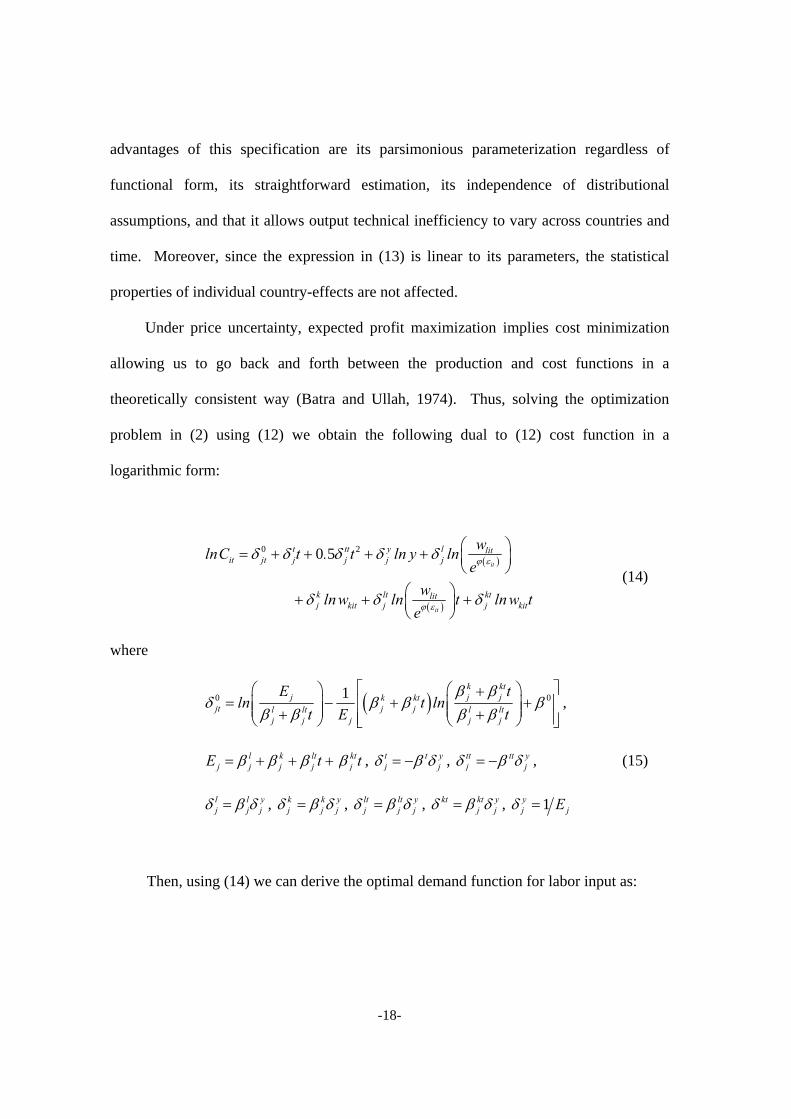
Under price uncertainty, expected profit maximization implies cost minimization

allowing us to go back and forth between the production and cost functions in a

theoretically consistent way (Batra and Ullah, 1974). Thus, solving the optimization

problem in (2) using (12) we obtain the following dual to (12) cost function in a

logarithmic form:

( )

( )

0 20 5it

it

t tt y l litit jt j j j j

k lt ktlitj kit j j kit

wlnC t . t ln y lne

w ln w ln t ln w te

ϕ ε

ϕ ε

δ δ δ δ δ

δ δ δ

⎛ ⎞= + + + + ⎜ ⎟⎝ ⎠

⎛ ⎞+ + +⎜ ⎟⎝ ⎠

(14)

where

( )0 01 k ktj j jk kt

jt j jl lt l ltj j j j j

E tln t ln

t E tβ β

δ β β ββ β β β

⎡ ⎤⎛ ⎞ ⎛ ⎞+= − + +⎢ ⎥⎜ ⎟ ⎜ ⎟⎜ ⎟ ⎜ ⎟+ +⎢ ⎥⎝ ⎠ ⎝ ⎠⎣ ⎦

,

l k ltj j j jE tβ β β= + + + kt

j tβ , t t yj jδ β δ= − , tt tt y

j jδ β δ= − , (15)

l l yj j jδ β δ= , k k y

j j jδ β δ= , lt lt yj j jδ β δ= , kt kt y

j jδ β δ= , 1yj jEδ =

Then, using (14) we can derive the optimal demand function for labor input as:

-19-

( ) ( )

0 20 5

it it

l ltj j* t tt y k

it jt j j j j kitlit

l lt ktlit litj j j kit

tlnl ln t . t ln y ln w

w

w w ln ln t ln w te eϕ ε ϕ ε

δ δδ δ δ δ δ

δ δ δ

⎛ ⎞+= + + + + +⎜ ⎟⎜ ⎟

⎝ ⎠⎛ ⎞ ⎛ ⎞+ + +⎜ ⎟ ⎜ ⎟⎝ ⎠ ⎝ ⎠

(16)

From (16) we can derive the compensated own- and cross-price elasticities of labor

demand, i.e.,

1*

d l ltitll j j

lit

lnle tln w

δ δ∂= = + −∂

(17)

and

*d k ktitlk j j

kit

lnle tln w

δ δ∂= = +∂

(18)

which are necessary for the estimation of the fifth term in (11). These demand elasticities

are both group and time-specific. Similarly the labor demand elasticity with respect to

human capital is obtained from:

( ) ( )*itd l ltit

l j j itlit it

lnle tlnε

ϕ εδ δ ε

ε ε∂∂

= = − +∂ ∂

(19)

that provides estimates of the fourth term in (11). The output cost elasticity necessary for

the estimation of the scale effect is obtained from:

-20-

C yity j

it

lnCln y

ε δ∂= =∂

(20)

The hypothesis of constant returns-to-scale can be statistically tested by imposing

the restriction that 1yj , jδ = ∀ which is equivalent with imposing linear homogeneity in

the aggregate production frontier given the restrictions in (15), i.e., 1l kj jβ β+ = and

0lt ktj j jβ β+ = ∀ . If this hypothesis cannot be rejected then the underlying technology

exhibits constant returns-to-scale and the second term in (11) vanishes.

For the estimation the technological change effects (third and last terms in (11)) we

need to compute the rate of cost diminution and the labor share equation. The former

under the multilateral generalized Cobb-Douglas specification in (14) is obtained,

( )it

t t tt lt ktit litit j j j j kit

lnC wC t ln ln wt eϕ εδ δ δ δ∂ ⎛ ⎞− = = + + +⎜ ⎟∂ ⎝ ⎠

(21)

The hypothesis of Hicks-neutral and zero technical change involves the following

parameter restrictions in (21): 0lt ktj jδ δ= = and 0t tt lt kt

j j j jδ δ δ δ= = = = j∀ ,

respectively.12 Accordingly, using the optimal labor share equation, i.e.,

l ltitlit j j

lit

lnCS tln w

δ δ∂= = +∂

(22)

we can compute the extended labor biased technical change effect as:

-21-

1 ltjlit

l ltlit j j

SS t t

δδ δ

∂=

∂ + (23)

Since the multilateral generalized Cobb-Douglas aggregate production model is

homothetic the second term in the extended labor biased technological change effect is

zero and therefore it does not contribute in labor productivity growth. If the underlying

aggregate production technology exhibits zero technical change then the third and the last

terms in (11) are zero and labor productivity growth is affected only from the remaining

four terms. If, however, technical progress is Hicks-neutral then only the extended labor

biased technical change effect vanishes. Finally, if the underlying technology is neutral

with respect to labor use, i.e., 0ltj jδ = ∀ , then again the final term in labor productivity

decomposition formula vanishes13.

Finally, for the estimation of the first term in (11) we need to compute labor

technical efficiency. For doing so we use Reinhard, Lovell and Thijssen (1999) approach

in the context of the multilateral generalized Cobb-Douglas production frontier.14

Conceptually, measurement of KPitLTE requires an estimate for the quantity it l itl lθ= ⋅

which is not observed. Substituting this into the aggregate production function model in

(12) and by noticing that the labor-specific technical efficient point lies on the frontier,

i.e., 0itξ = , relation (12) may be rewritten as:

( )( )

( )( )

0 20 5 it

it

t tt lit t j it

k lt ktj it j it j it it

ln y t . t ln l e

lnk ln l e t lnk t v

ϕ ε

ϕ ε

β β β β

β β β

= + + + ⋅

+ + ⋅ + + (24)

-22-

Since under weak monotonicity, output technical efficiency should imply and must

be implied by labor-specific technical efficiency, we can set the input specification in

(24) equal to the output-oriented specification in (12). Then, using the parameter

estimates obtained from the econometric estimation of the multilateral generalized Cobb-

Douglas production model and solving for itl , we can derive a measure of Kopp’s (1981)

non-radial labor-specific technical efficiency from the following relation (Reinhard

Lovell and Thijssen, 1999):15

KP itit l lt

j j

LTE expt

ξβ β

⎛ ⎞= −⎜ ⎟⎜ ⎟+⎝ ⎠

(25)

which is always different than zero as long as farms are technically inefficient from an

output-oriented perspective, i.e., 0itξ ≠ or 0 1 20 0 0i i i, ,ζ ζ ζ≠ ≠ ≠ i∀ . Using (13) and

(25) the time rate of change of labor technical efficiency is computed from:

( )( )

20 1 21 2

2

2lt

i i i jKP i iit l lt l lt

j j j j

t ttLTEt t

ζ ζ ζ βζ ζβ β β β

+ ++= − +

+ +

i

(26)

It is time-invariant if also output technical efficiency is time-invariant, i.e., 1 2 0i iζ ζ= =

i∀ and biased technical change is labor neutral, i.e., 0ltjβ = . It’s temporal pattern is

common across countries if 1 1i ,ζ ζ= 2 2iζ ζ= i∀ , l ljβ β= and lt lt

j jβ β= ∀ .

-23-

Labor allocative efficiency is then computed using the derived demand for labor

input in (16) and the labor technical efficient use, i.e., KPit it itl LTE l= × , as:

( )1

* itit it itl lt

j j

LAE l , y, ,t exp lt

ξεβ β

−⎡ ⎤⎛ ⎞

= − ×⎢ ⎥⎜ ⎟⎜ ⎟+⎢ ⎥⎝ ⎠⎣ ⎦w (27)

and it’s time rate of change is then computed using the time derivative of (16) and

relation (26) above as:

( ) ( )KP*it itit

it

ln LTE lln l , y, ,tLAE

t tε ∂ ×∂

= −∂ ∂wi

(28)

In effect it remains constant over time under zero technical change and time invariant

labor technical inefficiency, i.e., 1 2 0 i iζ ζ= = ∧ 0ltj jβ = ∀ and t tt lt

jβ β β= = =

0ktj jβ = ∀ , while it’s temporal pattern is common across countries if 1 1iζ ζ= ∧

2 2 i iζ ζ= ∀ and l ljβ β= , k k

jβ β= , lt ltjβ β= , kt kt

j jβ β= ∀ .

EMPIRICAL RESULTS

The fixed effects parameter estimates of the multilateral aggregate Cobb-Douglas

production frontier model in (12) are presented in Table 1 along with their corresponding

standard errors. The majority of the estimated parameters (except of two) were found to

be statistically significant at the 1 or 5 per cent level. All parameters have the anticipated

positive sign, while their magnitudes are bounded between 0 and 1 indicating that the

-24-

bordered Hessian matrix of first- and second-order partial derivatives is negative semi-

definite. This implies that all regularity conditions hold at the point of approximation,

i.e., positive and diminishing marginal productivities. In the lower panel of Table 1 are

also reported the country and time specific parameters of Cornwell et al., inefficiency

effects model in (13) for the country with the maximum efficiency score in each one of

the six groups. For the majority of the countries in the sample all parameters were found

to be positive (except of some African countries) implying improvements in output

technical efficiency over time (this finding is statistically examined next).16

Several hypotheses concerning the multilateral structure of the aggregate

production frontier model were tested using the generalized likelihood-ratio test statistic17

and the results are presented in the upper panel of Table 2. First, the hypothesis that the

imposed multilateral structure of the aggregate production frontier model in (12) is not

valid is rejected at the 5 per cent significance level (first hypothesis in table 2). Further,

the assumption that only the biases of technical change are similar across group of

countries is also rejected (second hypothesis in table 2). The same is true for the

marginal productivities of physical capital and labor inputs (third hypothesis in table 2).

Statistical testing results in the same conclusion when each one of the estimated

coefficients is tested separately (last four hypotheses). Hence, indeed data on inputs and

aggregate output in our sample are generated by multilateral models of production

supporting our initial hypothesis for approximating the worldwide production technology.

There are significant differences across group of countries in their respective choice of

production technology which should be taken into account in labor productivity growth

decomposition. Basu and Weil (1998) and Acemoglou and Zilibotti (2001),

-25-

appropriateness of technology paradigm is verified by the econometric estimation of our

aggregate production frontier.

The next set of hypotheses testing concerns the structure of technology, i.e.,

returns-to-scale and technical change. The results are presented in the middle panel of

Table 2. First, it seems that for every country group, the aggregate production technology

is not characterized by constant returns-to-scale as the relevant hypothesis was rejected at

the 5 per cent level, i.e., 1l kj jβ β+ = and 0lt kt

j jβ β+ = . This implies that the scale effect

is present constituting an important source of labor productivity growth. Average country

and time estimates of scale coefficients were found to be increasing for South and Central

American (1.0925), North America and Oceana (1.0412), Asian Tigers (1.2080) and

Europe (1.0141). On the other hand, African and Asian countries exhibit decreasing

returns as the relevant point estimates were found 0.9572 and 0.9573, respectively. This

implies that less developed countries in these two continents (i.e., Africa and Asia) have

gone beyond the potential capabilities of their aggregate own production technology.

The hypotheses of zero technical change i.e., 0lt ktT TT j jβ β β β= = = = and Hicks-

neutral technical change i.e., 0lt ktj j , jβ β= = ∀ were also rejected at the 5 per cent

significance level. On the average technical change was found progressive in all country

groups with the highest value being for Asian Tigers, 1.001 per cent. For North America

and Oceania the corresponding figure was 0.6076, for European countries 0.6909, for

South and Central American countries 0.5979, for African countries 0.6138 and for Asian

countries 0.7559. The parameters related with the neutral technical change, i.e., tβ and

ttβ , were found to be positive and statistically significant at the 1 per cent level, implying

-26-

that technical change was constantly progressive for the time period under consideration.

The second order parameters related with the biased part of technological change, i.e.,

ltjβ and kt

jβ were found to vary among the different groups of countries. Specifically,

technical change was found to be labor using in North America and Oceania and labor

saving in South and Central America, Africa, Asia and Asian Tigers, while the

corresponding parameter was found positive for Europe but statistically insignificant. On

the other hand, technical change was capital using in South and Central America, Africa,

and Asian Tigers and capital saving in Europe and North America and Oceania. The

relative parameter for Asia was found statistically insignificant. We have further

examined the hypothesis of labor-neutral technical change using the LR-test. The results

are in favour of labor-biased technical change rejecting the relevant hypothesis (last

hypothesis in the middle panel of table 2). Thus, the labor biased technical change effect,

i.e., first term in the last parenthesis in relation (11) is present and it should be taken into

consideration in the decomposition analysis of labor productivity growth.

The final set of statistical testing refers to the specification of labor technical and

allocative efficiency and it’s temporal pattern. First, countries in the sample are indeed

not exploiting full the potential of their aggregate production technology exhibiting

inefficiencies in resource utilization. These inefficiencies in labor use should be taken

into account when labor productivity growth is to be analyzed. Specifically the

hypothesis that all ζ parameters are jointly equal to zero is rejected at the 5 per cent level

of significance (first hypothesis in the lower panel of table 2). Further, labor technical

efficiency was found to be time varying during the 1965-90 period as the hypothesis that

1 2 0i iζ ζ= = and 0ltjβ = is also rejected at the same significance level (2nd hypothesis in

-27-

the lower panel). This temporal pattern of labor technical efficiency is not common

across countries in the sample, implying differences between countries in movements

towards their respective aggregate production frontier. Specifically the hypothesis that

1 1iζ ζ= , 2 2i iζ ζ= ∀ and l ljβ β= ∧ lt lt

j jβ β= ∀ is rejected from the generalized LR-

test (3rd hypothesis in the lower panel of the table). Concerning labor allocative

inefficiency, statistical testing implies that there are time varying labor utilization

mistakes at its technically efficient point. Finally, indeed countries in the sample are

making adjustments towards better utilization of labor under the prevailing factor prices

which are not common across countries in the sample (last two hypotheses in table 2).

Estimates of both labor technical and allocative efficiency in the form of frequency

distribution are reported in Table 3 for each group of countries. Estimated mean labor

technical efficiency over both countries and time was found to be 66.4 per cent. This

figure implies that the same level of aggregate output could have been produced on the

average, under the current technological conditions and physical capital use, if labor use

was decreased almost by 34 per cent. There is a notable difference on the average

efficiency scores between rich and poor group of countries. The most labor technically

efficient group was found to be Asian Tigers (87.81 per cent) followed by North America

and Oceania (79.42 per cent), and Europe (68.23 per cent). On the other hand, the less

labor technically efficient groups were South and Central America (63.88 per cent), Asia

(61.12 per cent) and Africa (44.75 per cent). Some of the Asian Tigers exhibit the

highest mean technical efficiency values (Thailand 90.59 per cent, Korea Rep 89.68 per

cent, Japan 87.64 per cent and Hong Kong 84.31 per cent) whereas African countries

-28-

have the lowest ones (Zambia 44.35 per cent, Zimbabwe 45.89 per cent, Malawi 45.38

per cent and Mauritius 47.04 per cent).

On the other hand, estimates of labor allocative efficiency further confirm this

divergence among poor and rich countries. In all three groups of developed countries

mean labor allocative efficiency is greater than unity indicating that labor is under-

utilized at its technical efficiency point compared with the groups of developing countries

where the corresponding figure is below one. Specifically, mean labor allocative

efficiency is 1.12 for North America and Oceania, 1.25 for Europe, and 1.32 for Asian

Tigers. Contrary, in South and Central America the corresponding figure is 0.66, 0.57 in

Africa and 0.67 in Asia. Israel and most European countries are underutilizing labor at its

technical efficient point having mean values well above unity (Israel 1.53, Belgium 1.56,

Ireland 1.40 and Denmark 1.41). On the other hand, India (0.34), Malawi (0.39), Turkey

(0.47) and Sri Lanka (0.47) seem to over-utilize extensively labor input.

Concerning the temporal pattern of these efficiency measures, the three less

efficient groups (South and Central America, Asia and Africa) were found to follow a

quite similar temporal pattern. As far as labor technical efficiency, all three groups were

found to follow an ascending path until 1975, followed by a constant decrease -except of

some slight upward variations- after this year. Only South and Central American

countries were found to present small improvements in their labor efficiency score at the

end of the period under consideration. The picture is different as regard allocative

efficiency scores. All three countries were found to follow an ascending temporal pattern

which was constantly sharper for Asian countries. On the other hand, North America and

Oceania and Europe were found to follow approximately a common path until the second

-29-

half of 70’s when European countries experienced a decrease in their labor technical

efficiency score. In the beginning of 80’s, North America and Oceania countries

overcame slightly the corresponding technical efficiency score of the European countries,

following however approximately a common path after this year. The results for the two

groups are similar, regarding labor allocative efficiency. Finally, Asian Tigers were

found to experience an increase in their labor technical efficiency score until 1975 which

is though lower than those of Europe and North America and Oceania. After a small

decrease in the second half of 70’s, Asian Tigers experienced an increase in labor

technical efficiency which was about two times higher than those of the other two

developed country-groups. As far as allocative efficiency, Asian Tigers were found to

follow a slightly descending path during the first five years, followed by a constant

increase until the end of the period. The highest rates of these improvements are observed

in the second half of 80’s.

Developing countries with low capital-labor mix seems to utilize more inefficiently

labor input compared with developed countries not exploring full the advantage of their

technological conditions. The appropriate technology paradigm of Basu and Weil (1998)

explains differences in the gap from the frontier among developed and developing

countries, but in a competitive economic environment exchange rate misalignments,

institutional features (e.g., rigidities in product and labor markets) and competitive

pressures affect the overall performance of individual economies. Further, the abundance

of labor input in developing countries results in over-utilization of its use in the

production process creating further inefficiency problems (e.g., India, Turkey and

Malawi). Finally, it is notable the fact that the variation on average labor technical

-30-

efficiency is higher for the groups of developing countries. It seems that some “rich”

developing countries have passed over some factor ratios and improved the technologies

specific to these ratios enhancing the utilization of their stock of labor (i.e., Mexico,

Colombia, Paraguay). This is also indicated by estimated mean labor allocative efficiency

values in Africa and South and Central America.

Table 4, reports the average values over countries and time of labor productivity

growth and it’s decomposition using relation (11). These figures are the weighted

averages computed following Olley and Pakes (1996) aggregation scheme. This is

actually a weighted average measure of worldwide labor productivity growth, using

countries’ output shares as weights. During the 1965-1990 time period, the weighted

average labor productivity growth was 1.431 per cent annually. The greatest part of that

labor productivity growth was due to TFP growth (75.76 per cent) and to a lesser extent

due to changes in factor intensities (15.45 per cent) and human capital accumulation (8.79

per cent). This finding is in accordance with the relevant literature that also attributes the

greatest share of productivity changes to TFP growth. Concerning the sources of TFP

growth, changes in the available technology (48.83 per cent) driven mainly by neutral

technical changes (45.04 per cent) and to a lesser extent due to factor biases (3.40 per

cent) are the most important factor accounting for that productivity growth. The effect of

scale economies and efficiency changes on labor productivity growth was found to be of

equal importance accounting for the 13.51 and 13.43 per cent of it, respectively.

Improvements in labor technical efficiency were more important indicating a trend

towards the respective technological frontier in each country. Still, however, the majority

-31-

of countries experienced a shift of the frontier rather than growth of their efficiency

scores.

In total, substitution effects (i.e., changes in capital-labor mix) were the second

highest source of that productivity growth accounting for the 15.45 per cent of it. Shifts

in relative capital-labor prices and the biases of technological change are important

possibilities for changes in the growth rate of factor intensities and the accumulation of

physical capital. The labor price effect (5.66 per cent) and the biased labor saving effect

(7.33 per cent) are dominant. The bias of technological change towards saving labor and

using capital is associated with the rising trend of labor price and the decline in the price

of capital. In this sense, the bias of technological change is consistent with the induced

innovation hypothesis (Hayami and Ruttan, 1970). Finally, human capital accumulation

accounts on the average for the 8.79 per cent of measured productivity growth. This is

mainly due to the high rates of growth in educational levels during 70’s in both developed

and developing countries.

Besides these average values it is also important to see the decomposition results

for each group of countries separately. Tables 5a and 5b present the decomposition of

labor productivity growth per group of country for the five sub-periods. The values

reported therein are the within groups weighted average for each sub-period. According

to these results Asian Tigers experienced the higher labor productivity growth during

1965-90 time period, 2.564 per cent, that is almost two times higher than the next two

groups of developed countries, namely North America and Oceania (1.352 per cent) and

Europe (1.218 per cent). South and Central America also experienced a high average

annual labor productivity growth, 1.232 per cent, driven mainly by scale economies and

-32-

technological improvements. On the other tail of the productivity distribution are African

and Asian countries that exhibit significant lower values, 0.886 and 1.004, per cent

respectively. Concerning the composition of these average values, productivity changes

rather than changes in factor intensities seems to dominate measured labor productivity

growth. There is only the exception of African countries where the contribution of

productivity changes accounts for the 52.60 per cent of that growth. Changes in relative

factor prices resulted to significant labor-saving technological improvements in these

countries given their input-mix which was abundant in labor input. Thus, the percentage

contribution of the extended labor saving technological change effect was the highest

among all groups of countries accounting for the 22.12 per cent of labor productivity

growth.

In Asian Tigers TFP accounts approximately for the 84.98 per cent of total labor

productivity changes whereas substitution effect only for the 11.43 per cent. The

contribution of human capital changes was the lowest among all groups of countries, 3.63

per cent (this figure is higher in Taiwan and Korea Rep.). These high TFP growth was

due to technological advances, 39.04 per cent, and the effect of scale economies, 39.47

per cent, (that was the highest scale effect among all groups). Korea Rep. and Taiwan

exhibit a very strong scale effect, whereas technological changes were significant in

Thailand, Japan and Korea Rep (see tables 6a and 6b). Given their factor endowments,

Asian Tigers seems to benefit a lot from exploring further the potential of their

technological conditions. They operate far below their minimum efficient size where the

average productivity of their resource endowments is maximized. Efficiency

improvements played an important role only in Japan, Taiwan and Thailand indicating

-33-

that only in these three countries significant movements towards the technological

frontier are observed. On the average improvements in labor technical and allocative

efficiency accounts only for the 6.48 per cent of productivity growth. Finally, changes in

factor intensities were also minor in labor productivity improvements, accounting for the

11.43 per cent.

In North America and Oceania changes in factor intensities and human capital

accumulation have a greater contribution in measured labor productivity growth. Still,

however, TFP changes account for the 71.60 per cent of labor productivity

improvements. Specifically, the human capital effect accounts for the 13.39 per cent of

measured productivity growth whereas the substitution effect for the 15.16 per cent.

Improvements in technical rather than in allocative efficiency are explaining the 12.80

per cent of total labor productivity (labor allocative accounts only for the 4.22 per cent of

total LP growth). Scale economies also have a minor contribution, 9.62 per cent, as all

countries operate close to maximizing average ray productivity. USA and Canada have

the highest annual productivity improvements, 1.370 and 1.323 per cent, respectively (see

tables 6a and 6b). In both countries, improvements in labor technical efficiency, human

capital accumulation and technological advances are the foremost important reasons of

the observed labor productivity growth.

Labor technical efficiency improvements are also important factor of labor

productivity growth for European countries. On the average labor technical efficiency

accounts for the 12.81 per cent of productivity improvements, while the corresponding

figure of labor allocative efficiency is only 2.22 per cent. In Switzerland, Denmark and

Netherlands technical efficiency changes are even higher than group average (see tables

-34-

6a and 6b). Given the input mix which is in favor of physical capital, developed

countries in both continents moved closer to their respective frontier as more cost

effective ways of improving their overall productivity rates. Still, however, technological

innovations account for the 56.73 per cent of total productivity rates, whereas the effect

of scale economies is also low, 3.53 per cent. In total TFP growth accounts for the 75.29

per cent of total labor productivity with insignificant variations among countries in the

group. On the other hand human capital accumulation accounts only for the 4.93 per

cent, whereas changes in factor intensities are significant as they contribute by 19.79 per

cent to total labor productivity growth. Changes in relative factor prices are the more

important source for the substitution effect. Netherlands, Austria and Sweden exhibit the

highest productivity rates among all European countries (1.454, 1.423 and 1.409,

respectively), whereas Italy (1.067 per cent), Germany (1.129 per cent) and UK (1.149

per cent) the lowest.

South and Central American countries present a similar picture in their

decomposition analysis. Specifically, the 74.35 per cent of measured labor productivity is

due to TFP, the 13.07 per cent to changes in factor intensities and the 12.66 per cent to

human capital accumulation. The latter is the third highest among all groups of countries

in the sample. The contribution of labor efficiency accounts for the 11.12 per cent with

both indices having and equal magnitude, 5.93 and 5.19 per cent for technical and

allocative efficiency, respectively. The effect of scale economies accounts for the 14.69

per cent of total labor productivity, higher than the European and North American and

Oceania countries. Caribbean and Central American countries exhibit the highest

productivity rates, Dominican Rep. 1.393 per cent, Guatemala 1.265 per cent, Honduras

-35-

1.321 per cent and Panama 1.243 per cent. In these countries, improvements in allocative

efficiency are more important than those of technical efficiency indicating better

adjustments of input mix relative to factor prices. This is in accordance with the

substitution effect whose contribution is increased for the countries with the highest

productivity rates in the group. Finally, no significant variation is observed on the

importance of technological innovations among South and Central American countries.

The effect of human capital accumulation was the highest in the group of Asian

countries accounting for the 15.94 per cent of total labor productivity. Still TFP accounts

for the 70.42 per cent and the substitution effect for the 13.75 per cent. Also changes in

input mix are towards improving allocation of physical capital and labor given the

prevailing factor prices as labor allocative efficiency has been considerably improved

over the period. On the average the effect of labor allocative efficiency accounts for the

11.65 per cent of measured productivity growth. This is the highest figure among all

groups. On the other hand movements towards the aggregate production frontier were

rather minor as the technically efficient effect was the 1.79 per cent of total labor

productivity. Finally, scale diseconomies combined with increased input use resulted in a

decrease of productivity rates by 18.33 per cent.

Finally, African countries exhibit the lowest labor productivity rates among all

groups with an average annual rate of only 0.886 per cent. Only the 52.60 per cent of it

arises from TFP growth and the 36.23 per cent from changes in factor intensities.

Mauritius and Malawi have the lowest productivity rates of 0.771 and 0.772 per cent,

respectively. On the other hand, Zambia and surprisingly Sierra Leone have the highest

mean values of 1.052 and 1.171 per cent, respectively. Like Asian countries, the scale

-36-

diseconomies accounted for a 17.72 per cent labor productivity slowdown during the

1965-90 period. It seems that both group of countries have gone beyond the potential

capabilities of their aggregate own production technology given their input-mix and

endowments. The striking result is that labor technical efficiency was deteriorated during

the period analyzed accounting for the 1.47 per cent productivity slowdown. However,

African countries seems to achieve a better input-mix given relative factor prices.

Finally, human capital accumulation is rather important indicating the gap of educational

levels in these countries.

Table 7 shows the decomposition of the average of labor productivity growth across

countries during the 1965-90 period. Labor productivity growth is following an

increasing pattern over time, experiencing however three falling sub-periods during 1970-

71, 1974-75 and 1981-1983 which were due to decreases in scale effect and human

capital effect that took place in these periods. The decreases in scale effect were caused

mainly by decreases in the relative output growth of many countries during the above-

mentioned periods which more or less coincide with the first oil crises. Moreover, as it

was expected, technical change was found to be constantly progressive over time, while

labor technical efficiency effect and substitution effect do not appear significant

variations during the period analyzed. The evolution of labor productivity growth for the

different groups of countries is illustrated in Figure 2. As we can observe, all groups seem

to have similar variations in labor productivity growth following an increasing trend.

However, we can notice two sharp decreases in labor productivity growth during the

years 1971 and 1975. The fall of labor productivity was found to be more intense for

Asian Tigers and African countries, while Asian countries seem to not have been

-37-

affected. During the first fifteen years, North America and Oceania group was found to

achieve greater labor productivity growth than Europe but after the early 80’s the

corresponding scores for the two groups were found to be quite similar.

CONCLUDING REMARKS

Motivated by the works of Färe et al., (1994), Kumar and Russell (2002) and Henderson

and Russell (2005), we provide a theoretically consistent parametric decomposition of

labor productivity growth. Relaxing the restrictive assumption of labor-specific technical

efficiency and incorporating human capital into our decomposition analysis we present a

detailed decomposition of labor productivity growth for a sample of developed and

developing countries drawn from Penn World Tables. Our empirical aggregate

production frontier model was based on the generalized Cobb-Douglas functional

specification suggested by Fan (1991) and was extended into a multilateral production

structure using Jorgenson and Nishimizu (1978) context of bilateral production functions.

The measurement of labor efficiency was based on Kopp’s (1981) orthogonal non-radial

index of factor-specific technical efficiency modified in a parametric frontier framework.

Finally, following Griliches (1963), human capital proxied by Hall and Jones (1999)

construction was introduced into the analysis as a multiplicative augmentation of labor

input.

Our empirical results confirms that Basu and Weil (1998) and Acemoglou and

Zilibotti (2001) appropriateness of technology paradigm as the hypothesis of a common

worldwide aggregate production technology does not fit data of our sampled countries.

Each continent seems to have different technological conditions that should be taken into

-38-

account in productivity analysis. TFP growth accounts for the greatest share of labor

productivity with significant variations though among group of countries. On the average

countries in the sample experienced an average labor productivity growth of 1.4309 per

cent annually. Asian Tigers, North America and Oceania and Europe exhibit the highest

labor productivity changes whereas, for African and Asian countries the corresponding

figures were significantly lower. In developed countries, changes in labor efficiency

seems to be important source explaining that productivity differentials, while human

capital accumulation had an important effect in developing countries productivity

improvements. In African countries labor utilization have been deteriorated as technical

efficiency of labor was decreased over time. Still changes in technological conditions are

the foremost important sources of productivity growth mainly in developing countries

that accounted approximately for the 65 per cent of that growth.

-39-

REFERENCES

Abramovitz, M. (1986). Catching up, Forging Ahead, and Falling Behind. Journal of

Economic History, 46: 385-406.

Acemoglou, D and F. Zilbotti (2001). Productivity Differences. Quarterly Journal of

Economics 116: 563-606.

Akridge, J.T. (1989). Measuring Productive Efficiency in Multiple Product Agribusiness

Firms: A Dual Approach. American Journal of Agricultural Economics 71: 116-

125.

Antle, J.M. and S.M. Capalbo (1988). An Introduction to Recent Development in

Production Theory and Productivity Measurement. In: Agricultural Productivity:

Measurement and Explanation. Resources for the future, Inc., Washington, DC.

Atkinson, S.E., and C. Cornwell (1998). Estimating Radial Measures of Productivity

Growth: Frontier vs Non-Frontier Approaches. Journal of Productivity Analysis 10:

35-46.

Badunenko, O., Hennderson, D.J. and V. Zelenyuk (2008). Technological Change and

Transition: Relative Contributions to Worldwide Growth During the 90s. Oxford

Bulletin of Economics and Statistics, 70: 461—492.

Barro, R.J. and J.W. Lee. (1993). International Comparisons of Educational Attainment.

Journal of Monetary Economics 32: 363-394.

Barro, R.J. and J.W. Lee. (2001). International Data on Educational Attainment: Updates

and Implication. Oxford Economic Papers 53: 541-563.

-40-

Bartel, A.P. and F.R. Lichtenberg (1987). The Comparative Advantage of Educated

Workers in Implementing New Technology. Review of Economics and Statistics,

69: 1-11.

Basu, S. and D.N. Weil (1998). Appropriate Technology and Growth. Quarterly Journal

of Economics, 113: 1025-1054.

Batra, R.N. and H. Ullah (1974). Competitive Firm and the Theory of the Input Demand

under Uncertainty. Journal of Political Economy 82: 537-548.

Becker, G.S. (1975). Human Capital: A Theoretical and Empirical Analysis. Columbia

University Press: New York.

Benhabib, J., and M.M. Spiegel (1994). The Role of Human Capital in Economic

Development: Evidence from Aggregate Cross-Country and Regional U.S. Data,

Journal of Monetary Economics, 34: 143–73.

Bils, M., and P.J. Klenow (2000). Does Schooling Cause Growth? American Economic

Review, 90: 1160–83.

Blackorby, C., C.A.K. Lovell, and M.C. Thursby (1976). Extended Hicks Neutral

Technological Change. Economic Journal 86: 845-52.

Caselli, F. (2005). Accounting for Cross-Country Income Differences. In Aghion, P.,

Durlauf, S. (eds), Handbook of Economic Growth, Elsevier: Amsterdam.

Cornwell, C., Schmidt, P. and R.C. Sickles (1990). Production Frontiers with Cross-

sectional and Time-series Variation in Efficiency Levels. Journal of Econometrics

46: 185-200.

-41-

Fan, S. (1991). Effects of Technological Change and Institutional Reform on Production

Growth in Chinese Agriculture. American Journal of Agricultural Economics 73:

266-275.

Fan, S. and P.G. Pardey (1997). Research, Productivity, and Output Growth in Chinese

Agriculture. Journal of Development Economics 53: 115-137.

Färe, R., Grosskopf, S., Noris, M. and Z. Zhang (1994). Productivity Growth, Technical

Progress and Efficiency Change in Industrialized Countries. American Economic

Review, 84: 66-83.

Gollin, D. (2002). Getting Income Shares Right. Journal of Political Economy 110: 458–

474.

Griliches, Z. (1963). Estimates of the Aggregate Agricultural Production Function from

Cross-Sectional Data. Journal of Farm Economics XLV: 1411-1427.

Griliches, Z. (1964). Research Expenditures, Education, and the Aggregate Agricultural

Production Function. American Economic Review, LIV: 961-974.

Griliches, Z. (1970). Notes on the Role of Education in Production Functions and

Growth Accounting. In Education, Income and Human Capital, W.L. Hansen (ed.),

UMI Press, Cambridge, MA: U.S.A..

Hall, R.E. and C.I. Jones (1999). Why Some Countries Produce so Much More Output

per Worker than Others? Quarterly Journal of Economics 114: 83-116.

Hayami, Y. and V.W Ruttan (1970). Agricultural Productivity Differences Among

Countries. American Economic Review 60: 895-911.

Henderson D.J. and R.R. Russell (2005). Human Capital and Convergence: A Production

Frontier Approach. International Economic Review 46:1167-1205.

-42-

Jorgenson, D.W. and B.M. Fraumeni (1993). Education and Productivity Growth in a

Market Economy. Atlantic Economic Journal, 21: 1-25.

Jorgenson, D.W. and M. Nishimizu (1978). US and Japanese Economic Growth, 1952-

1974: An International Comparison. Economic Journal 88, 707-726.

Kopp, R.J. (1981). The Measurement of Productive Efficiency: A Reconsideration.

Quarterly Journal of Economics 96: 477-503.

Krusell, P., and J.V. Rios-Rull (1996). Vested Interests in a Positive Theory of Stagnation

and Economic Growth. Review of Economic Studies, 63: 301-329.

Kumar, S. and R.R. Russell (2002). Technological Change, Technological Catch-Up, and

Capital Deepening: Relative Contributions to Growth and Convergence. American

Economic Review 92: 527-548.

Kuroda, Y. (1987). The Production Structure and Demand for Labor in Postwar Japanese

Agriculture. American Journal of Agricultural Economics 69: 326-337.

Kuroda, Y. (1995). Labor Productivity Measurement in Japanese Agriculture, 1956-1990.

Journal of Agricultural Economics 12: 55-68.

Los, B. and M.P. Timmer (2005). The Appropriate Technology Explanation of

Productivity Growth: An Empirical Approach. Journal of Development Economics,

77: 517-531.

Lucas, R.E. (1988). On the Mechanisms of Economic Development. Journal of Monetary

Economics, 22: 3-42.

Mamuneas, T., Savvides, A. and T. Stengos (2006). Economic Development and the

Return to Human Capital: A Smooth Coefficient Semiparametric Approach.

Journal of Applied Econometrics 21: 111-132.

-43-

O’Neil, D. (1995). Education and Income Growth: Implications for Cross-Country

Inequality, Journal of Political Economy, 103: 1289–1301.

Olley, G.S. and A. Pakes (1996). The Dynamics of Productivity in the

Telecommunications Equipment Industry. Econometrica 64: 1263-1297.

Olson, M. (1982). The Rise and Decline of Nations: Economic Growth, Stagflation and

Social Rigidities. Yale University Press.

Parente, S.L. and E.C. Prescott (1999). Monopoly Rights: A Barrier to Riches. American

Economic Review, 89: 1216-1233.

Prescott, E.C. (1988). Needed: A Theory of Total Factor Productivity. International

Economic Review, 39: 525-552.

Psacharopoulos, G. (1994). Returns to Investment in Education: A Global Update. World

Development 22: 1325-43.

Ray, S.C. (1998). Measuring Scale Efficiency from a Translog Production Function.

Journal of Productivity Analysis 11: 183-194.

Reinhard, S., C.A.K. Lovell, and G. J. Thijssen (1999). Econometric Estimation of

Technical and Environmental Efficiency: An Application to Dutch Dairy Farms.

American Journal of Agricultural Economics 81: 44-60.

Romer, P.M. (1990). Endogenous Technological Change. Journal of Political Economy,

98: S71-S102.

Schmidt, P. and C.A.K. Lovell (1980). Estimating Stochastic Production and Cost

Frontiers when Technical and Allocative Inefficiency are Correlated, Journal of

Econometrics 13: 83-100.

-44-

Schmidt, P. and R.C. Sickles (1984). Production Frontiers and Panel Data. Journal of

Business and Economic Statistics 2: 367-374.

Schultz, T.W. (1961). Investment in Human Capital. American Economic Review, 51: 1-

17.

Solow, R.M. (1957). Technical Change and the Aggregate Production Function. Review

of Economics and Statistics, 39: 312-320.

Welch, F. (1970). Education in production. Journal of Political Economy 80: 35-59.

-45-

Figure 1. Measurement of Labor Specific Technical and Allocative Efficiency.

A

l

k

0l 1l

0k

O

B

y( )C ,y, ,tεw

C

*l

*k

-46-

Table 1. Parameter Estimates of the Multilateral Cobb-Douglas Production Frontier.

Par. N. America&Oceania S.&C. America Europe Africa Asia Asian Tigers

Estimate StdError

Common Coefficient Estimates 0β 0.6469 (0.0350)* tβ 0.1250 (0.0151)* ttβ 0.0356 (0.0042)*

Estimate StdError Estimate StdError Estimate StdError Estimate StdError Estimate StdError Estimate StdError Multilateral Structure

lβ 0.4234 (0.1879)* 0.5783 (0.3408)** 0.3943 (0.0478)* 0.4627 (0.0428)* 0.5768 (0.0742)* 0.7403 (0.0814)* kβ 0.6182 (0.1500)* 0.5138 (0.0256)* 0.6162 (0.0278)* 0.4921 (0.0213)* 0.3728 (0.0520)* 0.4848 (0.0343)* ltβ 0.2795 (0.0540)* -0.0240 (0.0114)* 0.0060 (0.0092) -0.0772 (0.0416)** -0.0457 (0.0094)* -0.0849 (0.0161)* ktβ -0.2780 (0.0542)* 0.0226 (0.0075)* -0.0203 (0.0083)* 0.0673 (0.0260)* 0.0144 (0.0133) 0.1542 (0.0112)*

0iζ 0.9523 (0.0180)* 0.9070 (0.0148)* 0.9798 (0.0160)* 0.7928 (0.0207)* 0.9107 (0.0496)* 0.9205 (0.0199)*

1iζ 0.6439 (0.0156)* 0.6854 (0.0288)* 0.6568 (0.0118)* 0.6310 (0.0402)* 0.6360 (0.0187)* 0.5636 (0.0192)*

2iζ 0.3563 (0.0088)* 0.3149 (0.0163)* 0.3434 (0.0066)* 0.3694 (0.0227)* 0.3644 (0.0105)* 0.3374 (0.0108)* 2R 0.4690

Note: l refers to labor, c to capital and, t to time. In the lower panel of the table are reported the ζ parameters of the country with the maximum efficiency score. * and ** indicate statistical significance at the 1 and 5 per cent level, respectively.

-47-

Table 2. Model Specification Tests.

Hypothesis LR-test Critical Value (a=0.05)

Multilateral Structure Testing l lj β β= , k k

j β β= , lt ltj β β= and kt kt

jβ β= 37.61 24 9.49χ =

lt ltj β β= and kt kt

jβ β= 25.69 22 5.99χ =

l lj β β= and k k

j β β= 23.40 22 5.99χ =

l lj β β= 14.26 2

1 3.84χ =

k kj β β= 16.30 2

1 3.84χ =

lt ltj β β= 12.55 2

1 3.84χ =

kt ktj β β= 13.21 2

1 3.84χ =

Technological Specification

Constant returns-to-scale: 1l kj j β β+ = ∧ 0lt kt

j j jβ β+ = ∀ 64.20 22 5.99χ =

Hicks-neutral technical change: 0lt ktj j jβ β= = ∀ 49.28 2

2 5.99χ =

Zero-technical change: 0t tt lt ktj j jβ β β β= = = = ∀ 75.60 2

4 9.49χ =

Labor-neutral technical change: 0ltj jβ = ∀ 13.78 2

1 3.84χ =

Inefficiency Specification

Existence of inefficiency: 0 1 2 0 i i i iζ ζ ζ= = = ∀ 144.58 2156 71.52χ ≈

Time-invariant labor technical efficiency: 1 2 0 i iζ ζ= = ∧ 0ltj jβ = ∀ 123.21 2

105 69.92χ ≈

Common temporal pattern of labor technical efficiency across countries: 1 1iζ ζ= ∧ 2 2 i iζ ζ= ∀ and l l

jβ β= ∧ lt ltj jβ β= ∀ 106.37 2

106 70.34χ ≈

Time-invariant labor allocative efficiency: 1 2 0 i iζ ζ= = ∧ 0ltj jβ = ∀ and

0t tt lt ktj j jβ β β β= = = = ∀

198.42 2109 71.33χ ≈

Common temporal pattern of labor allocative efficiency across countries: 1 1iζ ζ= ∧ 2 2 i iζ ζ= ∀ and l l

jβ β= , k kjβ β= , lt lt

jβ β= , kt ktj jβ β= ∀ 174.57 2

108 71.05χ ≈

-48-

Table 3. Frequency Distribution of Labor-Specific Technical and Allocative Efficiency.

% N. America&Oceania S.&C. America Europe Africa Asia Asian Tigers All Countries

Labor Specific Technical Efficiency <40 0 0 0 0 0 0 0

40-50 0 0 0 6 0 0 6

50-60 0 1 1 0 3 0 5

60-70 0 12 12 0 2 0 26

70-80 1 0 5 0 1 0 7

80-90 3 0 0 0 0 4 7

90> 0 0 0 0 0 1 1

Mean 79.4 63.9 68.2 44.9 61.1 87.8 66.4

Min 72.3 58.9 56.1 44.3 51.2 84.3 44.3

Max 83.5 69.9 74.8 47.0 74.9 90.6 90.6 Labor Specific Allocative Efficiency

<0.5 0 0 0 1 4 0 5

0.5-0.75 0 12 1 4 0 0 17

0.75-1.0 1 1 0 1 1 0 4

1.0-1.25 1 0 6 0 0 1 8

1.25-1.5 2 0 10 0 0 4 16

1.5> 0 0 1 0 1 0 2

Mean 1.12 0.66 1.25 0.57 0.67 1.32 0.95

Min 0.81 0.51 0.56 0.40 0.35 1.23 0.35

Max 1.31 0.80 1.56 0.75 1.53 1.45 1.56

N 4 13 18 6 6 5 52

-49-

Table 4. Decomposition of Labor Productivity Growth (average values over countries and time).

Annual Rate (%)

Labor Productivity Growth 1.431 (100.0)

Changes in Labor Technical Efficiency 0.140 (9.80)

Changes in Allocative Efficiency 0.052 (3.63)

Scale Effect 0.193 (13.51)

Rate of Technical Change: 0.699 (48.83)

Autonomous Part 0.647 (45.04)

Biased Part 0.052 (3.40)

Human Capital Effect 0.126 (8.79)

Substitution Effect: 0.221 (15.45)

Price Effect: 0.116 (8.12)

Physical Capital 0.035 (2.46)

Labor 0.081 (5.66)

Extended Labor Biased TC Effect 0.105 (7.33)

Note: The average rate of labor productivity change was calculated using Olley and Pakes (1996) output share weighting. The values in parenthesis indicate the percentage contribution of each effect to labor productivity change.

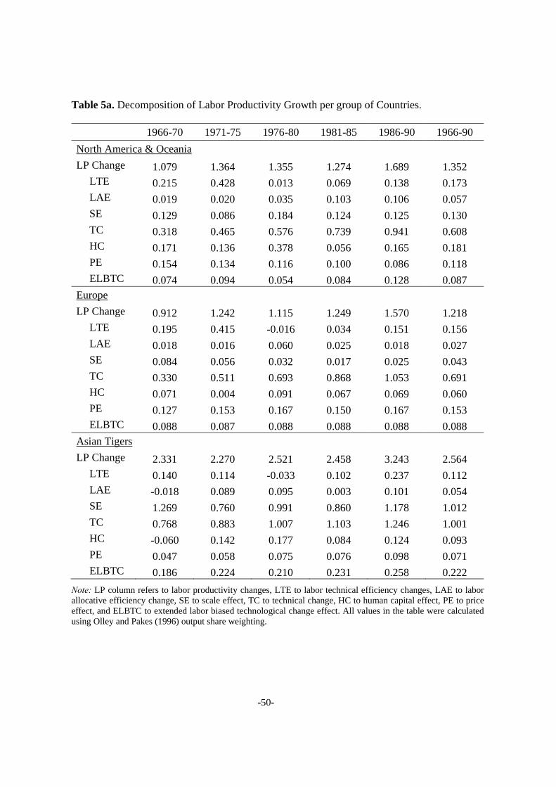
-50-

Table 5a. Decomposition of Labor Productivity Growth per group of Countries.

1966-70 1971-75 1976-80 1981-85 1986-90 1966-90 North America & Oceania LP Change 1.079 1.364 1.355 1.274 1.689 1.352

LTE 0.215 0.428 0.013 0.069 0.138 0.173 LAE 0.019 0.020 0.035 0.103 0.106 0.057 SE 0.129 0.086 0.184 0.124 0.125 0.130 TC 0.318 0.465 0.576 0.739 0.941 0.608 HC 0.171 0.136 0.378 0.056 0.165 0.181 PE 0.154 0.134 0.116 0.100 0.086 0.118 ELBTC 0.074 0.094 0.054 0.084 0.128 0.087

Europe LP Change 0.912 1.242 1.115 1.249 1.570 1.218

LTE 0.195 0.415 -0.016 0.034 0.151 0.156 LAE 0.018 0.016 0.060 0.025 0.018 0.027 SE 0.084 0.056 0.032 0.017 0.025 0.043 TC 0.330 0.511 0.693 0.868 1.053 0.691 HC 0.071 0.004 0.091 0.067 0.069 0.060 PE 0.127 0.153 0.167 0.150 0.167 0.153 ELBTC 0.088 0.087 0.088 0.088 0.088 0.088

Asian Tigers LP Change 2.331 2.270 2.521 2.458 3.243 2.564

LTE 0.140 0.114 -0.033 0.102 0.237 0.112 LAE -0.018 0.089 0.095 0.003 0.101 0.054 SE 1.269 0.760 0.991 0.860 1.178 1.012 TC 0.768 0.883 1.007 1.103 1.246 1.001 HC -0.060 0.142 0.177 0.084 0.124 0.093 PE 0.047 0.058 0.075 0.076 0.098 0.071 ELBTC 0.186 0.224 0.210 0.231 0.258 0.222

Note: LP column refers to labor productivity changes, LTE to labor technical efficiency changes, LAE to labor allocative efficiency change, SE to scale effect, TC to technical change, HC to human capital effect, PE to price effect, and ELBTC to extended labor biased technological change effect. All values in the table were calculated using Olley and Pakes (1996) output share weighting.

-51-

Table 5b. Decomposition of Labor Productivity Growth per group of Countries.

1966-70 1971-75 1976-80 1981-85 1986-90 1966-90 South and Central America LP Change 0.961 1.053 1.291 1.242 1.614 1.232

LTE 0.111 0.245 -0.012 -0.018 0.037 0.073 LAE 0.062 0.038 0.072 0.067 0.081 0.064 SE 0.157 0.078 0.303 0.192 0.176 0.181 TC 0.267 0.433 0.599 0.763 0.928 0.598 HC 0.202 0.083 0.158 0.081 0.258 0.156 PE 0.111 0.125 0.121 0.102 0.081 0.108 ELBTC 0.052 0.052 0.051 0.055 0.054 0.053

Africa LP Change 0.529 0.669 0.950 0.994 1.290 0.886

LTE 0.058 0.080 -0.083 -0.079 -0.042 -0.013 LAE 0.030 0.021 0.006 0.031 0.022 0.022 SE -0.120 -0.198 -0.156 -0.125 -0.184 -0.157 TC 0.205 0.406 0.624 0.814 1.021 0.614 HC 0.061 0.057 0.227 0.022 0.133 0.100 PE 0.122 0.131 0.145 0.113 0.113 0.125 ELBTC 0.175 0.173 0.187 0.217 0.227 0.196

Asia LP Change 0.762 0.935 0.925 1.079 1.320 1.004

LTE 0.141 0.121 -0.088 -0.064 -0.022 0.018 LAE 0.113 0.091 0.119 0.124 0.139 0.117 SE -0.135 -0.130 -0.153 -0.224 -0.279 -0.184 TC 0.368 0.557 0.749 0.951 1.156 0.756 HC 0.151 0.151 0.162 0.152 0.185 0.160 PE 0.027 0.036 0.035 0.033 0.030 0.032 ELBTC 0.098 0.109 0.102 0.108 0.113 0.106

Note: LP column refers to labor productivity changes, LTE to labor technical efficiency changes, LAE to labor allocative efficiency change, SE to scale effect, TC to technical change, HC to human capital effect, PE to price effect, and ELBTC to extended labor biased technological change effect. All values in the table were calculated using Olley and Pakes (1996) output share weighting.

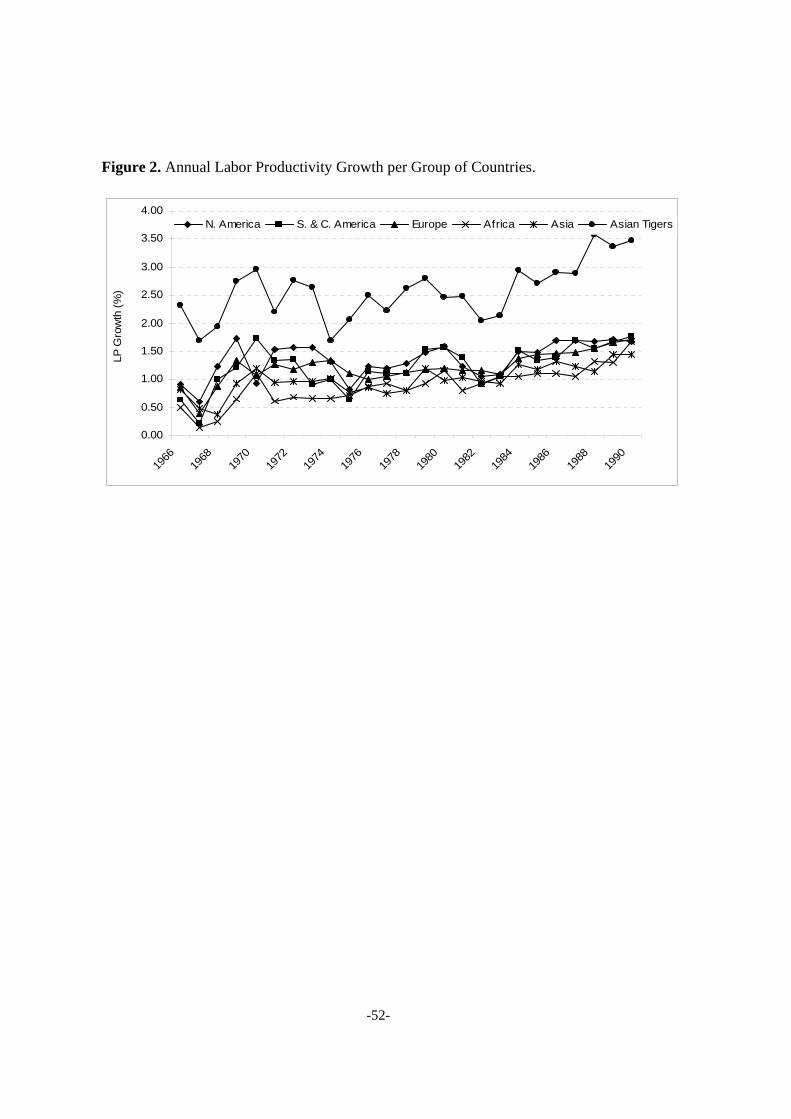
-52-

Figure 2. Annual Labor Productivity Growth per Group of Countries.

0.00

0.50

1.00

1.50

2.00

2.50

3.00

3.50

4.00

1966

1968

1970

1972

1974

1976

1978

1980

1982

1984

1986

1988

1990

LP G

row

th (%

)

N. America S. & C. America Europe Africa Asia Asian Tigers

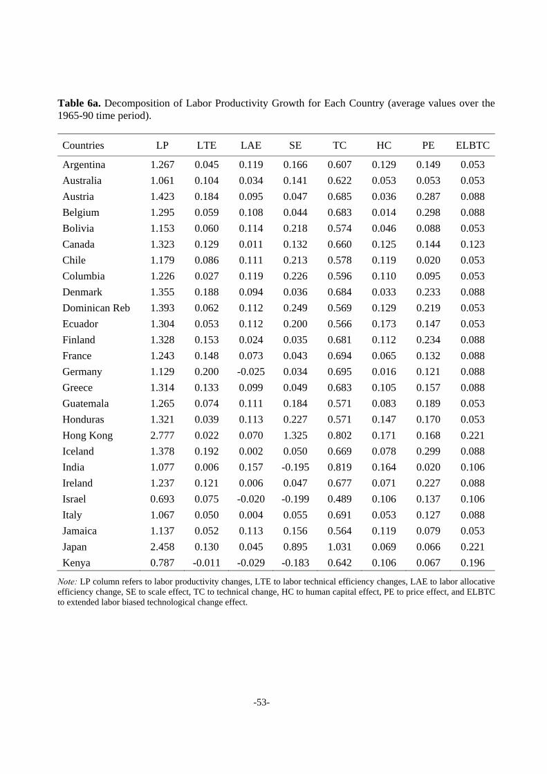
-53-

Table 6a. Decomposition of Labor Productivity Growth for Each Country (average values over the 1965-90 time period).

Countries LP LTE LAE SE TC HC PE ELBTC

Argentina 1.267 0.045 0.119 0.166 0.607 0.129 0.149 0.053 Australia 1.061 0.104 0.034 0.141 0.622 0.053 0.053 0.053 Austria 1.423 0.184 0.095 0.047 0.685 0.036 0.287 0.088 Belgium 1.295 0.059 0.108 0.044 0.683 0.014 0.298 0.088 Bolivia 1.153 0.060 0.114 0.218 0.574 0.046 0.088 0.053 Canada 1.323 0.129 0.011 0.132 0.660 0.125 0.144 0.123 Chile 1.179 0.086 0.111 0.213 0.578 0.119 0.020 0.053 Columbia 1.226 0.027 0.119 0.226 0.596 0.110 0.095 0.053 Denmark 1.355 0.188 0.094 0.036 0.684 0.033 0.233 0.088 Dominican Reb 1.393 0.062 0.112 0.249 0.569 0.129 0.219 0.053 Ecuador 1.304 0.053 0.112 0.200 0.566 0.173 0.147 0.053 Finland 1.328 0.153 0.024 0.035 0.681 0.112 0.234 0.088 France 1.243 0.148 0.073 0.043 0.694 0.065 0.132 0.088 Germany 1.129 0.200 -0.025 0.034 0.695 0.016 0.121 0.088 Greece 1.314 0.133 0.099 0.049 0.683 0.105 0.157 0.088 Guatemala 1.265 0.074 0.111 0.184 0.571 0.083 0.189 0.053 Honduras 1.321 0.039 0.113 0.227 0.571 0.147 0.170 0.053 Hong Kong 2.777 0.022 0.070 1.325 0.802 0.171 0.168 0.221 Iceland 1.378 0.192 0.002 0.050 0.669 0.078 0.299 0.088 India 1.077 0.006 0.157 -0.195 0.819 0.164 0.020 0.106 Ireland 1.237 0.121 0.006 0.047 0.677 0.071 0.227 0.088 Israel 0.693 0.075 -0.020 -0.199 0.489 0.106 0.137 0.106 Italy 1.067 0.050 0.004 0.055 0.691 0.053 0.127 0.088 Jamaica 1.137 0.052 0.113 0.156 0.564 0.119 0.079 0.053 Japan 2.458 0.130 0.045 0.895 1.031 0.069 0.066 0.221 Kenya 0.787 -0.011 -0.029 -0.183 0.642 0.106 0.067 0.196

Note: LP column refers to labor productivity changes, LTE to labor technical efficiency changes, LAE to labor allocative efficiency change, SE to scale effect, TC to technical change, HC to human capital effect, PE to price effect, and ELBTC to extended labor biased technological change effect.

-54-

Table 6b. Decomposition of Labor Productivity Growth for Each Country (average values over the 1965-90 time period).

Countries LP LTE LAE SE TC HC PE ELBTC

Korea Rep 3.028 0.035 0.027 1.552 0.903 0.221 0.070 0.221 Malawi 0.772 -0.039 0.037 -0.175 0.619 0.055 0.079 0.196 Mauritius 0.771 -0.029 0.072 -0.124 0.534 0.104 0.018 0.196 Mexico 1.180 0.096 0.012 0.142 0.605 0.192 0.081 0.052 Netherlands 1.454 0.218 0.060 0.046 0.686 0.113 0.244 0.088 New Zealand 1.314 0.216 0.055 0.079 0.640 0.174 0.023 0.128 Norway 1.298 0.104 0.001 0.048 0.684 0.146 0.227 0.088 Panama 1.243 0.079 0.026 0.173 0.550 0.160 0.203 0.052 Paraguay 1.165 0.090 0.032 0.134 0.571 0.136 0.150 0.052 Peru 1.312 0.086 0.043 0.227 0.590 0.165 0.149 0.052 Philippines 0.907 0.005 0.063 -0.140 0.671 0.165 0.038 0.106 Portugal 1.350 0.176 0.006 0.055 0.683 0.100 0.243 0.088 Sierra Leone 1.171 -0.031 0.022 -0.079 0.661 0.044 0.356 0.196 Spain 1.370 0.263 0.033 0.050 0.685 0.093 0.157 0.088 Sri Lanka 0.775 -0.007 0.049 -0.148 0.609 0.097 0.070 0.106 Sweden 1.409 0.182 0.038 0.039 0.688 0.048 0.327 0.088 Switzerland 1.331 0.267 0.037 0.031 0.684 0.069 0.155 0.088 Syria 0.837 0.000 0.005 -0.111 0.503 0.217 0.118 0.106 Taiwan 3.017 0.037 0.142 1.430 0.851 0.204 0.130 0.221 Thailand 2.692 0.056 0.125 1.160 0.959 0.131 0.040 0.221 Turkey 0.869 0.080 0.028 -0.167 0.645 0.141 0.036 0.106 UK 1.149 0.138 0.006 0.036 0.695 0.075 0.111 0.088 USA 1.370 0.180 0.062 0.129 0.602 0.193 0.120 0.084 Yugoslavia 1.277 0.141 0.098 0.053 0.688 0.097 0.113 0.088 Zambia 1.052 0.016 0.047 -0.095 0.580 0.128 0.179 0.196 Zimbabwe 0.939 -0.004 0.061 -0.162 0.604 0.113 0.131 0.196 Mean 1.431 0.140 0.052 0.193 0.699 0.126 0.116 0.105

Note: LP column refers to labor productivity changes, LTE to labor technical efficiency changes, LAE to labor allocative efficiency change, SE to scale effect, TC to technical change, HC to human capital effect, PE to price effect, and ELBTC to extended labor biased technological change effect.

-55-

Table 7. Annual Decomposition of Labor Productivity Growth (weighted average over countries)

Note: LP column refers to labor productivity changes, LTE to labor technical efficiency changes, LAE to labor allocative efficiency change, SE to scale effect, TC to technical change, HC to human capital effect, PE to price effect, and ELBTC to extended labor biased technological change effect. All values in the table were calculated using Olley and Pakes (1996) output share weighting.

Year LP LTE LAE SE TC HC PE ELBTC 1966 1.002 0.209 0.036 0.179 0.298 0.114 0.123 0.043 1967 0.600 -0.192 0.006 0.150 0.333 0.114 0.122 0.068 1968 1.104 0.104 0.025 0.251 0.368 0.112 0.121 0.123 1969 1.603 0.530 0.054 0.248 0.404 0.111 0.121 0.135 1970 1.287 0.287 0.001 0.247 0.440 0.109 0.119 0.085 1971 1.458 0.456 0.056 0.169 0.469 0.088 0.120 0.102 1972 1.515 0.387 0.004 0.262 0.503 0.088 0.122 0.149 1973 1.512 0.385 0.026 0.249 0.542 0.088 0.127 0.097 1974 1.335 0.404 0.053 0.004 0.571 0.088 0.127 0.090 1975 1.064 0.110 0.032 0.021 0.598 0.088 0.121 0.095 1976 1.276 -0.072 0.072 0.220 0.619 0.219 0.120 0.098 1977 1.240 -0.040 0.005 0.207 0.654 0.220 0.119 0.074 1978 1.354 -0.018 0.037 0.223 0.691 0.221 0.121 0.078 1979 1.534 0.026 0.094 0.242 0.724 0.220 0.124 0.103 1980 1.522 0.035 0.095 0.198 0.755 0.218 0.124 0.097 1981 1.376 0.042 0.074 0.168 0.786 0.073 0.116 0.117 1982 1.217 0.050 0.044 0.017 0.816 0.074 0.109 0.109 1983 1.230 -0.131 0.054 0.177 0.854 0.074 0.105 0.097 1984 1.652 0.127 0.083 0.267 0.890 0.074 0.104 0.109 1985 1.615 0.130 0.055 0.223 0.928 0.074 0.101 0.104 1986 1.747 0.149 0.066 0.185 0.968 0.136 0.106 0.139 1987 1.766 0.130 0.029 0.232 1.007 0.136 0.108 0.124 1988 1.873 0.137 0.061 0.266 1.047 0.136 0.110 0.116 1989 1.933 0.130 0.110 0.231 1.082 0.136 0.108 0.136 1990 1.968 0.130 0.128 0.208 1.120 0.136 0.108 0.137 Mean 1.431 0.140 0.052 0.193 0.699 0.126 0.116 0.105

-56-

ENDNOTES

1 Labor-specific technical efficiency as defined in (3), has an input conserving interpretation, which

however cannot be converted into a cost-saving measure due to its non-radial nature. Akridge (1989)

based on Kopp’s (1981) theoretical framework incorporated factor prices suggesting a single factor

technical cost efficiency index which measures the potential cost savings that can be realized by

adjusting single factor use.

2 If labor input is under-utilized at it’s technical efficient point, the second term of the efficiency

effect is positive (negative) as labor allocative efficiency decreases (increases) over time. In this case

in the measurement of labor productivity growth the correct direction has been accounted for.

3 The maintained assumption that derived demand for labor is non-increasing in ε, implies that human

capital and labor inputs are substitutes in the production of aggregate output (Griliches, 1964).

4 Our data set is the same with that used by Henderson and Russell (2005) and to some extent with

Kumar and Russell (2002) and so our results are comparable with those reported by these two

studies.

5 Aggregate output is real gross domestic product multiplied by population while capital stock and

labor inputs were retrieved from capital stock per worker and real GDP per worker. All variables are

measured in 1985 international prices.

6 Data obtained by National Account Statistics of the UN do not take into consideration self-

employment. To deal with this, the number of self employed workers was computed as a proportion

of the total number of employees, and then labor compensation was calculated by assuming that

employees and self-employed workers receive the same wages on average (Gollin, 2002). Then we

calculated labor compensation by multiplying the share of employee compensation, i.e., ls , in

national income with the product of GDP price i.e., YP , times the GDP. The remaining portion of this

-57-

product, i.e., ( ) ( )1 l Ys P GDP− × × , was the corresponding value for physical capital. Then, we

constructed a price index for labor by dividing labor compensation by the number of workers from

Penn World Tables, i.e., ( )l l Yw s P GDP l⎡ ⎤= × ×⎣ ⎦ . The constructed price index for labor was

converted to constant 1985 US dollars using PPP for labor in each country which was computed by

dividing the labor cost per worker at the base year by the corresponding value in the US. The same

approach was conducted for the calculation of the price of capital at constant 1985 US dollars.

7 Using the years of schooling for adult population is a good proxy for human capital given the

difficulties of alternative data source. As Griliches (1963) pointed out the use of “specific” or more

elegant variables does not alter significantly the econometric results as all these variables are highly

correlated with years of schooling.

8 Given that Barro and Lee (1993; 2001) data are available in five years intervals while the rest of out

data are on annual basis, we assume a constant annual rate of growth for human capital within each

interval.

9 This specification implicitly imposes perfect substitutability between human capital and physical

labor (Acemoglou and Zilboti, 2001). Alternatively we could have follow Welch (1970) approach

treating human capital as a separate factor of production. Following Griliches (1970) we used formal

statistical testing to examine both hypotheses. In doing so the production frontier model in (12) was

estimated using human capital as a separate factor of production. Then using a simple t-test we

examined the hypothesis that the coefficients of human capital and labor are equal. The result rejects

the alternative hypothesis validating our choice of using education as an augmentation factor for

physical labor in the production frontier model.

-58-

10 We have tried to introduce the multilateral structure into the temporal pattern of output technical

inefficiency, but unfortunately we couldn’t obtain statistical significant estimates.

11 This means that in each period at least one country is fully efficient, although the identity of this

country may vary through years.

12 Given (15) this is equivalent by testing the hypotheses that 0lt ktj jβ β= = and t tt

j jβ β= =

0lt ktj jβ β= = j∀ in the aggregate production function in (12).

13 Again given (15) this is equivalent by testing the hypotheses that 0ltjβ = in the aggregate

production function in (12).

14 In fact Ray (1998) based on Atkinson and Cornwell’s (1998) findings suggested a similar approach

with Reinhard Lovell and Thijssen (1999) for the estimation of input specific technical efficiency.

15 Reinhard, Lovell and Thijssen (1999) in developing their approach of measuring Kopp’s (1981)

orthogonal input-specific technical efficiency correctly argued that under a Cobb-Douglas

specification of the production function, both indices will exhibit the same ranking for countries in

the sample. However, this is not true with the multilateral generalized Cobb-Douglas production

model utilized herein which allows for different temporal patterns among the two efficiency

measures for countries belonging to different groups as well as across time.

16 The complete set of parameter estimates for the Cornwell et al., (1990) inefficiency effects model

are available upon request.

17 The generalized likelihood-ratio test statistic is computed as: ( ) ( ){ }0 12LR ln L H ln L H= − − ,

where ( )0L H and ( )1L H denote the values of the likelihood function under the null ( )0H and the

alternative ( )1H hypothesis, respectively.