declination (b1950) 13 12 smm3 smm5 … (b1950) right ascension (b1950) 18 27 45 30 15 00 01 16 15...

DE

CL

INA

TIO

N (

B1

95

0)

RIGHT ASCENSION (B1950)18 27 45 30 15 00

01 16

15

14

13

12

11

10

09

08

0 5 10

SMM1S68FIRS1

SMM2

SMM3

SMM4

SMM5

SMM6

S68N

On The Fly Observing at the 12 Meter

Je� Mangum([email protected])

September 21, 1999

Contents

1 Introduction 3

1.1 When to OTF Map . . . . . . . . . . . . . . . . . . . . . . . . . . . . . 3

1.2 How OTF Observing Works . . . . . . . . . . . . . . . . . . . . . . . . 4

1.3 An Important Note About Spatial Sampling . . . . . . . . . . . . . 5

1.4 Other Sources of Information . . . . . . . . . . . . . . . . . . . . . . . 6

2 Observing Setup 6

2.1 OTF Observing Checklist . . . . . . . . . . . . . . . . . . . . . . . . . 6

2.2 OTF Map Parameters . . . . . . . . . . . . . . . . . . . . . . . . . . . . 7

2.2.1 Row Sampling Rate . . . . . . . . . . . . . . . . . . . . . . . . . . . 7

2.2.2 Scanning Rate . . . . . . . . . . . . . . . . . . . . . . . . . . . . . . 8

2.2.3 Row Length Limitations . . . . . . . . . . . . . . . . . . . . . . . . 9

2.2.4 Bad Channel Flagging . . . . . . . . . . . . . . . . . . . . . . . . . 9

2.2.5 Map RMS . . . . . . . . . . . . . . . . . . . . . . . . . . . . . . . . 9

2.2.6 Total Map Time . . . . . . . . . . . . . . . . . . . . . . . . . . . . 12

2.2.7 Doppler Tracking . . . . . . . . . . . . . . . . . . . . . . . . . . . . 12

2.2.8 Examples . . . . . . . . . . . . . . . . . . . . . . . . . . . . . . . . 13

2.3 OTF Map Setup . . . . . . . . . . . . . . . . . . . . . . . . . . . . . . . 13

2.4 Data File Management . . . . . . . . . . . . . . . . . . . . . . . . . . . 18

3 On-Line Data Monitoring 19

3.1 Dataserve . . . . . . . . . . . . . . . . . . . . . . . . . . . . . . . . . . . 19

3.2 Databrowse . . . . . . . . . . . . . . . . . . . . . . . . . . . . . . . . . . 21

4 UniPops 21

4.1 Spectral Line . . . . . . . . . . . . . . . . . . . . . . . . . . . . . . . . . 21

4.2 Continuum . . . . . . . . . . . . . . . . . . . . . . . . . . . . . . . . . . . 23

1

5 OFF Scan Editing Utilities 23

6 AIPS Processing 24

6.1 Spectral Line . . . . . . . . . . . . . . . . . . . . . . . . . . . . . . . . . 25

6.1.1 Shotgun Analysis . . . . . . . . . . . . . . . . . . . . . . . . . . . . 25

6.1.2 Step-By-Step Analysis . . . . . . . . . . . . . . . . . . . . . . . . . 31

6.1.3 Combining Multiple Maps . . . . . . . . . . . . . . . . . . . . . . . 34

6.1.4 Spatial Smoothing . . . . . . . . . . . . . . . . . . . . . . . . . . . 36

6.2 Continuum . . . . . . . . . . . . . . . . . . . . . . . . . . . . . . . . . . . 36

6.3 More Extensive Processing . . . . . . . . . . . . . . . . . . . . . . . . 38

6.3.1 Integrated Intensity Images . . . . . . . . . . . . . . . . . . . . . . 38

6.3.2 Gaussian Fits . . . . . . . . . . . . . . . . . . . . . . . . . . . . . . 39

6.3.3 Displaying Your Data . . . . . . . . . . . . . . . . . . . . . . . . . . 40

2

1 Introduction

On-the- y (OTF) mapping is an observing technique in which the telescope is drivensmoothly and rapidly across a �eld while data and antenna position information arerecorded continuously. This technique is in contrast to traditional mapping of discretepositions on the sky, which is sometimes called \step-and-integrate" or \point-and-shoot"mapping. There are several advantages to OTF mapping. First, telescope overhead isreduced signi�cantly since a speci�c position on the sky does not have to be acquiredwithin a given tolerance. Second, since the entire �eld is covered rapidly, properties ofthe atmosphere and the system, including antenna pointing and calibration, change less incomparison to a conventional point-and-shoot map. Systematic changes may occur frommap to map, but such e�ects average down rapidly and may be correctable by cross corre-lation techniques. In general, global changes from map to map are more benign and easierto correct than drifts across a single map �eld.

OTF mapping is available at the 12 Meter for spectral line and continuum measure-ments. OTF is not a new concept and has been used at a number of radio telescopes invarying forms for many years. Nevertheless, given the rigor of the position encoding thatallows precise and accurate gridding of the data, the fast data recording rates that allowrapid scanning without beam smearing, and the analysis tools that are already available orare under development, we believe that the 12 Meter implementation is the most ambitiouse�ort at OTF imaging yet.

1.1 When to OTF Map

In principle, the OTF technique should be a superior way to make almost any map. It isparticularly eÆcient for large �elds and relatively strong emission. In these cases, one gainsconsiderable observing time from the low telescope overhead. We strongly recommend OTFmapping in these cases. OTF can, and has, been used to advantage for small �elds andweaker lines. For small �elds, however, the telescope must turn around at the end of a rowmore often. Weak lines may require many, many coverages of the �eld that can lead to asubstantial data reduction chore requiring many hours of your time and a fast computerwith gigabytes of disk space. This is a judgement the observer must make. Note thataside from the minimum hardware integration period imposed by the backends, all OTFintegrations are done in post-processing analysis software rather than by the real-timesystems.

Spectral line OTF guidelines are arbitrary, but we would recommend that for any �eld> 60 in width, you should most de�nitely use OTF. OTF may be entirely appropriatefor smaller �elds, but the advantages may not be as marked. If the �eld is only a fewgrid points across, you should probably use conventional grid mapping. If the emission isweak, you may elect to use a slow scanning rate to reduce the number of �eld coveragesrequired. Be advised that the OTF technique is constantly evolving. Observing options are

3

being enhanced, computers are being upgraded, and analysis software is being developed.Accordingly, the criteria for choosing which observing algorithm to use is also evolving.Check with us before planning your observations.

1.2 How OTF Observing Works

Before starting an OTF map, you con�gure the telescope control system for the widthof the �eld, the scanning rate, the row spacing, and a few other things. For spectralline OTF, the map is taken in a total power observing mode in the sense that you takea calibration spectrum (a vane CAL) and a total power OFF, followed by one or moretotal power scanning rows, typically made up of hundreds of individual spectra (the ONs).For continuum OTF, the map is acquired using the continuum beam-switched observingmode. In this mode, the subre ector is switched between two positions (the \+" and \-"beam) in azimuth while the telescope scans. Each of the individual spectra or continuum\+" and \-" beam total power measurements is tagged with the actual antenna encoderpositions. As a result, antenna tracking errors caused by wind gusts, for example, areactually recorded and taken into account in the data analysis stage.

For spectral line OTF, the same CAL and OFF are used to calibrate all of the ONs inthe scanning rows until another OFF is taken. Each total power OFF is given its own scannumber. All of the spectra or continuum \+" and \-" beam total power measurements ineach scanning row are concatenated along with arrays of time and position information andstored on disk under a single scan number with a single header. The header informationfor each scanning row contains the scan number of the previous OFF (for spectral lineOTF) and CAL.

Given the scanning parameters, the positioning system is con�gured for tracking rates,row o�sets, and the duration of a scanning row. The spectral line data-taking backendtells the tracking system to move to position and begin scanning. Using some handshakingbits on the telescope's status and monitor (SAM) bus, the two systems are synchronizedat the start of each row. In addition, both the tracking and backend computers haveIRIG clock cards that are driven by the observatory rubidium standard clock. The databackend reads out the spectrometers system every 100 milliseconds for spectral line OTF.The continuum data system is read out every 250 milliseconds. For both spectral lineand continuum OTF, the data backend tags each data parcel with the UT time stamp.Since the Millimeter Autocorrelator (MAC) is a digital autocorrelation device, before thedata can be read out Fourier transforms of the 100 millisecond data samples are required.To make data analysis as fast as possible, the FFT's are performed in real-time by theMAC control computers. Every 10 milliseconds, the tracking computer records its Az/Elposition with respect to the �eld center. At the end of the scanning row, the positioninformation from the tracking system is merged with the data. An interpolation of theposition information is done to align slight di�erences between the time stamps of the twodata sets.

4

1.3 An Important Note About Spatial Sampling

The following is due to Darrel Emerson

When setting up your map observations, it is important to keep in mind the followingfacts about sampling and aliasing in radio astronomical mapping data. If you want torepresent the full resolution of the telescope, you have to sample the data often enough torepresent all the spatial frequencies detected by the dish. You can think of the extremeedges of the dish of diameter D as part of an interferometer of spacing D, which has tobe sampled at �

2D. Depending on the illumination taper, this corresponds typically to

sampling at about 2.4 or 2.5 points per FWHM. Of course, if there is zero, or by somede�nition \negligible", illumination at the edge of the dish, you won't be sensitive to suchhigh spatial frequencies. It will be just the same as a smaller dish of diameter d equal tothe diameter of that part of the dish that has signi�cant illumination, and the samplingwill be calculated from �

2X, where X is de�ned as the diameter of the illuminated part of

the surface.

It's useful to consider what happens if you undersample data. Assume that the un-dersampling happens on the sky, rather than in later in the data processing. Suppose youhave a 10m dish, but you only sample at �

2�8mrather than the �

2�10mthat you should.

That means that the spatial frequencies present from the dish baselines of 8m to 10mget re ected back into the spatial frequencies of 8m down to 6m. Not only have spatialfrequencies from the 8m to 10m baselines been lost, but valid spatial frequencies frombaselines of 6m to 8m have been corrupted. You can't tell if structure in your map with aspatial wavelength of �

7mis genuine, or was really structure at �

9mwhich has been aliased

on top of any genuine �7m

spatial wavelength signal. In this sense, undersampling the skyis really twice as bad as you might have thought.

How important this undersampling is depends on exactly what the illumination taperis, how important it is that you retain the maximum possible resolution of the telescope,how good a dynamic range you want in the observations, and at some level how much�ne scale structure there is in the source itself. If you only sample at 0.8 Nyquist (e.g.FWHM

2rather than FWHM

2:5), what matters is the energy in the data at spatial wavelengths

shorter than �2�0:8�D

. So in a sense you need to ask what the illumination taper is at aradius of 0:4�D on the dish surface. The spatial frequency response of a single dish is theautocorrelation function of the voltage illumination pattern. So, you need to calculate howmuch area there is under the 2-D autocorrelation function beyond spatial frequencies of0:8�D, compared to the area within 0:8�D. This ratio is some measure of the dynamicrange. A better de�nition of dynamic range might take into account the spatial frequencystructure of the source. If the source has no structure on scales smaller than �

2�0:8�D, then

you don't need to sample at the full �2�D

anyway.

This is one circumstance where it is perfectly rigorous to undersample the data. If, say,you have a 10m dish, and you are taking data to compare with other observations using a1m dish at the same wavelength (or the equivalent number of wavelengths at some other

5

frequency) then you only need to sample the data at �2�5:5m

or �11m

. This is so because,when sampling a 10m dish as if it were a 5.5m dish, the spatial frequency components frombaselines of 5.5m out to 10m will be re ected back into the data as if corresponding tobaselines of 5.5m down to 1m. So, the spatial frequency terms of 1m baseline and belowwill not have been corrupted. The data analysis of this undersampled data would applya spatial frequency cuto� at 1m, and there will have been no corruption in this smootheddata caused by the undersampling. Putting it in more general terms, if you are going tobe smoothing a dish of diameter D to simulate observations made with a smaller dish ofdiameter d, then the sampling interval only needs to be �

d+Drather than �

2�D.

There are other aspects that make it desirable to sample more often than the Nyquistrate, as we recommend for OTF observing. These are practical points like how well grid-ding or interpolation works with a �nite sized gridding or interpolation function. A littleoversampling may enable you to reduce the convolution (interpolation) function by a factorof a few, saving a huge amount of computational overhead at the expense of a few per centmore data.

1.4 Other Sources of Information

� D. T. Emerson, \Increasing the Yield of our Telescopes", in Proceedings to IAU 170,CO: 25 Years of Millimeter-Wavelength Spectroscopy.

� E. Greisen, \Single-Dish Data in Aips", Chapter 10, AIPS Cookbook.

� J. G. Mangum, D. T. Emerson, & E. Greisen, \The On-The-Fly Observing Technique",in Proceedings to Imaging at Radio through Submillimeter Wavelengths.

2 Observing Setup

2.1 OTF Observing Checklist

The following list gives some step-by-step instructions which you can use as a guide toacquiring and processing OTF data. In each item, I indicate the appropriate section whichyou should refer to for further information.

� For Spectral Line OTF...

Have the operator con�gure the �lter bank, MAC, and position-switch parametersfor your measurements.

Test the system by having the operator make a short position-switched measure-ment of a strong source in the �eld you are going to map.

6

Use your test measurement to identify and ag any bad �lter bank channels (x2.2.4).For Both Spectral Line and Continuum OTF...

Tell the telescope operator that you will be doing OTF mapping. You will need tospecify the map setup parameters (x2.3).

Start a new data �le for each new map coverage.

Once the map has begun, adjust the Dataserv parameters to get the best on-linedisplay (x3.1).

Use the AIPS procedures OTFSET and OTFRUN to read and process your com-pleted map (x6.1.1).

Run the Unix shell script datacomp to compress your raw data �les (x2.4).Check the raw and AIPS disk status with the disk space monitor (select \Diskspace"

in the obs \Observer Tools" menu). If you reach the point where you need towrite data to tape, use the tar utility (x2.4).

2.2 OTF Map Parameters

In the following I describe some of the OTF map parameters which you must calculate inorder to setup your OTF observing.

2.2.1 Row Sampling Rate

It is very important that you set up your map to be properly sampled perpendicular to thescanning direction. If you under sample, you will miss information in the image �eld, youwill be unable to accurately combine your image with that from interferometers or othersingle-dish telescopes, and you may introduce artifacts from the analysis algorithms. Keepin mind that you can always smooth the map after it is taken to degrade the resolutionand improve signal-to-noise.

The scanning rows must be spaced at no more than the Nyquist spacing, which is alsoknown as \critical sampling" and is given by

�N � �obs2D

' 2576:53

�obs(GHz)

for a 12m aperture. In practice, though, a small amount of oversampling is recommended.If the rows are critically spaced, small scanning errors can result in the map being undersampled. In addition, the tail of the gridding function used by the analysis procedure

7

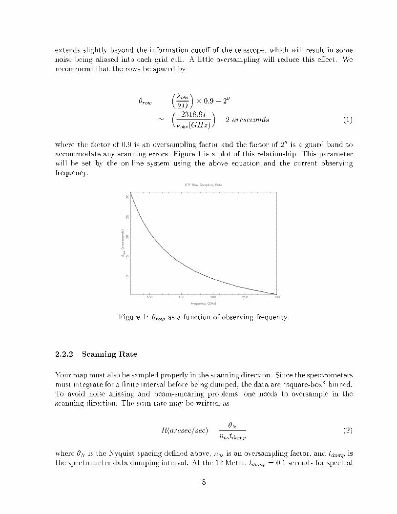
extends slightly beyond the information cuto� of the telescope, which will result in somenoise being aliased into each grid cell. A little oversampling will reduce this e�ect. Werecommend that the rows be spaced by

�row =��obs2D

�� 0:9� 200

'�

2318:87

�obs(GHz)

�� 2 arcseconds (1)

where the factor of 0.9 is an oversampling factor and the factor of 200 is a guard band toaccommodate any scanning errors. Figure 1 is a plot of this relationship. This parameterwill be set by the on-line system using the above equation and the current observingfrequency.

Figure 1: �row as a function of observing frequency.

2.2.2 Scanning Rate

Your map must also be sampled properly in the scanning direction. Since the spectrometersmust integrate for a �nite interval before being dumped, the data are \square-box" binned.To avoid noise aliasing and beam-smearing problems, one needs to oversample in thescanning direction. The scan rate may be written as

R(arcsec=sec) =�N

nostdump(2)

where �N is the Nyquist spacing de�ned above, nos is an oversampling factor, and tdump isthe spectrometer data dumping interval. At the 12 Meter, tdump = 0.1 seconds for spectral

8

line OTF, 0.25 seconds for continuum OTF. We recommend a minimum value for nos of2, which will result in < 3% increased noise as a result of aliasing and minimal beambroadening. Note that it is quite acceptable to oversample by much larger factors than theminimum value suggested above, particularly in the scanning direction. There are sometradeo�s to be considered, however. Large factors of oversampling will produce bettersignal-to-noise on a single coverage of the �eld and may result in simpler data processing,i.e. fewer maps to average together. On the other hand, the longer a single coverage takes,the more susceptible your image will be to drifts in the system, such as pointing andatmosphere. This eliminates some of the advantages of fast mapping mentioned above. Asa compromise, we recommend that the row spacing be computed from Equation 1, andthat the scan rate follow from Equation 2, with nos > 2. Other circumstances may comeinto play, of course. For example, if the �eld size is very small, you may choose to slowthe scan rate (increase nos) substantially.

2.2.3 Row Length Limitations

Since the telescope acquires a data sample every 0.1 (spectral line) or 0.25 (continuum)seconds, the combination of the telescope slew rate and the scan length in RA determineshow much data you get per row. Due to software and practical restrictions, the maximumnumber of samples one can acquire in a given scan is 3600. This corresponds to a slew rateof 10 arcseconds/second over a scan which is 1Æ in length. You should set your observingparameters to stay below the 3600 spectra per row limit.

2.2.4 Bad Channel Flagging

It is a good idea to ag bad �lter bank channels before processing the data in AIPS.Therefore, before you begin your OTF map, identify any bad �lter bank channels by makinga normal position-switched test measurement of your source. Use the badch procedure inunipops to identify the bad channels and tell the operator that you want these channelsto be agged. If you forget to ag some bad channels, you will have to use the chanseladverb in OTFUV (see x6.1.2).

2.2.5 Map RMS

When planning an OTF observing run you must calculate how much integration time youneed for each sampling cell to reach the desired signal-to-noise level. First determine theintegration time required using the standard Radiometer Equation

spec�cell =T �sysp

��spectcell

"1 +

spectcelltoff

#1=2(for spectral line)

9

cont�cell = something (for continuum) (3)

where T �sys is the e�ective system temperature, �� is the spectral resolution, tcell is the

time spent integrating on a cell, and toff is the o�-source integration time. For spectral lineOTF, the time spent integrating on a given cell is typically one second or less, while the o�-source integration time is typically 10 seconds (the default value). Therefore, tcell � toffand we can rewrite the spectral line Radiometer Equation as

spectcell =1

��

T �sys

�cell

!2

(4)

The integration time in a map cell is a function of the scanning rate and the number ofcoverages of the map �eld, and should be calculated with respect to the time accumulatedin a Nyquist sampling cell. Figure 2 shows some of the terms I will de�ne below.

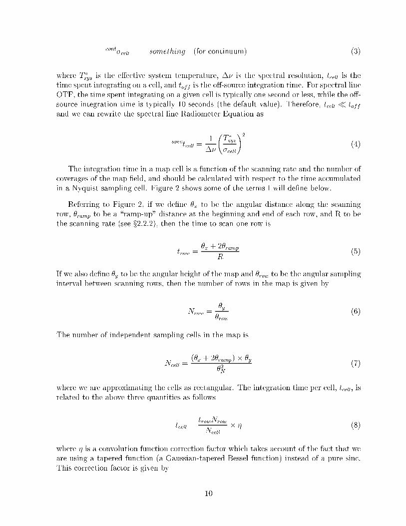
Referring to Figure 2, if we de�ne �x to be the angular distance along the scanningrow, �ramp to be a \ramp-up" distance at the beginning and end of each row, and R to bethe scanning rate (see x2.2.2), then the time to scan one row is

trow =�x + 2�ramp

R(5)

If we also de�ne �y to be the angular height of the map and �row to be the angular samplinginterval between scanning rows, then the number of rows in the map is given by

Nrow =�y�row

(6)

The number of independent sampling cells in the map is

Ncell =(�x + 2�ramp)� �y

�2N(7)

where we are approximating the cells as rectangular. The integration time per cell, tcell, isrelated to the above three quantities as follows

tcell =trowNrow

Ncell� � (8)

where � is a convolution function correction factor which takes account of the fact that weare using a tapered function (a Gaussian-tapered Bessel function) instead of a pure sinc.This correction factor is given by

10

θx

θramp

{θramp

{θy

θrow {

Figure 2: Map parameter de�nitions.

� =

RFFT (Gauss�Bessel) dxdyR

FFT (sinc) dxdy

' 2:9135 (9)

for the truncated functions we use in the AIPS task SDGRD (see x6.1.2). CombiningEquations 5, 6, 7, 8, and 9, we �nd that

tcell =2:9135�2NR�row

(10)

Combining this relation for tcell with our Radiometer Equation (Equation 4), we �nd that

11

the RMS noise per cell in an OTF map is given by

�cell =T �sys

�N

R�row

2:9135��

! 1

2

(11)

Note that a given RMS noise per cell obtainable with multiple coverages and/or polariza-tions is given by

� =�cellpNc

(12)

where Nc is the number of coverages and/or polarizations you combine to produce your�nal image. Note that you can also improve your map RMS by spatially smoothing it aftergridding (see x6.1.4).

2.2.6 Total Map Time

The total time required to acquire a map must include not only the integration timescanning across the �eld but also the time for calibration and OFF integrations. This canbe written as

specttot = Nrow

"trow +

toffNrpo

+tcal

NrpoNopc+

�

Nrpo

#(for spectral line)

contttot = Nrowtrow (for continuum) (13)

where Nrow is the number of rows in the map, trow is given by Equation 5 above, toff isthe OFF integration time, tcal is the calibration integration time (VANE plus SKY sampletimes), Nrpo is the number of rows per OFF measurement you do, Nopc is the numberof OFF measurements per calibration measurement you make, and � is the \overhead"time, which is the time that the telescope spends doing things other than integrating (likemoving from OFF positions to the map �eld). The value for � depends mainly on howfar away the OFF position is from the map, but 10 seconds is probably a good averageestimate. The CAL is taken at the same position and just before the OFF, and so doesn'tinvolve additional overhead. There may be other small overhead losses in moving from rowto row and starting scans, but these losses can usually be neglected.

2.2.7 Doppler Tracking

The default reference position for doppler tracking of OTF maps is the map center position.It is possible to change these settings to doppler track relative to any RA and Dec.

12

2.2.8 Examples

Spectral Line:

In early September of 1995 I made a map of the J=1! 0 C18O transition toward theSerpens star formation region. The rest frequency for this transition is 109.782160 GHz,which means that the Nyquist sampling rate was 2300 (Equation 1) and the row separationwas 2000 (Equation 1). I mapped a �eld 300 � 300 in size, which meant that my map had90 rows. I scanned at a rate of 50 arcsec/sec, which gave me an oversampling factor of4.6 (Equation 2). I used the default ramp-up distance of 10, which means that each rowtook 38.4 seconds to acquire (Equation 5). Given these map parameters, the number ofindependent sampling cells in the map was 6,533 (Equation 7). The system temperaturewas about 300 K while the �lter resolution was 100 kHz. Therefore, from Equation 11 wecalculate that �cell ' 0:76K for a single-polarization map. I actually did this map twice,both times with dual polarization, so that the resultant rms in my map will be about 0.38K (Equation 12). This estimate compares quite favorably to the measured rms of � 0.37K.

Continuum:

Coming soon...

2.3 OTF Map Setup

When you give your map setup parameters to the operator, he will �ll-in a menu likethe one shown in Figures 3 and 4. In the following, I describe each of these parametersand indicate how they should be set for both types of OTF map. I have also written aprogram called MAPCALC which will calculate your OTF map RMS given your inputmap parameters. This program is available on any of the 12 Meter Telescope computersand is also available by request from Je� Mangum.

OFF Integration Time: (spectral line only) This is the time spent acquiring OFF posi-tion measurements. The default value of 10 seconds is good for almost all situations.

CAL Integration Time: This is the time spent acquiring a vane calibration measure-ment. The default value of 5 seconds is good for almost all situations.

OFF Type: (spectral line only) You can choose between relative (PS) or absolute (APS)OFF position measurements. If you use APS, you must have an OFF source positionaccessible from your source catalog.

Rows per OFF: (spectral line only) The default value is 1, but under almost all circum-stances it will be more eÆcient to use 2. If you use 2, you should make sure that youuse the OFF-interpolation feature of the OTFUV task in AIPS to assign the closestOFF measurement in time to your ON scans. Larger numbers of rows per o� should

13

Figure 3: Spectral line OTF observing setup screen.

14

Figure 4: Continuum OTF observing setup screen.

15

only be done under the very best of weather conditions at 3mm, and rarely if everat 1mm.

Rows per Cal: (continuum only) The default value is 1, which is probably the best valueto use under all conditions.

OFF's per CAL: (spectral line only) This should be left at the default value of 1 sincecalibration measurements involve a minimal amount of overhead.

Scan Coordinate: This is the coordinate in which the map rows will be acquired. Forspectral line OTF you can scan in either RA, Dec, lII, or bII, while in continuumOTF the scan directions are Az and El.

Angle: (spectral line only) This is the angle relative to the scanning coordinate enteredabove that you want to have the telescope scan.

Map Size in RA(L): (spectral line only) This is your map dimension in RA or lII ex-cluding the rampup distance.

Map Size in DEC(B): (spectral line only) This is your map dimension in DEC or bIIexcluding the rampup distance.

Map Size in AZ: (continuum only) This is your map dimension in Az excluding therampup distance.

Map Size in EL: (continuum only) This is your map dimension in El excluding the ram-pup distance.

Scan Rate (arcsec/sec): Since the resultant map RMS noise level at a given observingfrequency and spectral resolution is given by

� /s

R

Nc

(14)

(see Equations 11 and 12), your target map RMS noise level can be achieved by slowscanning rates and fewer coverages or faster scanning rates and a larger number ofcoverages. When setting R, you should:

1. Measure at least 2 data samples per Nyquist interval (see x2.2.2). Note thatat 230 GHz the maximum scanning rate is 5600/sec for spectral line OTF, and??00/sec for continuum OTF.

2. Calibrate often enough so that the sky doesn't vary signi�cantly between yourON and associated OFF source measurements (for spectral line OTF) or duringa row (for continuum OTF). This time should be less than 2 minutes at 3mmand less than 1 minute at 1mm, with shorter intervals necessary under poorerweather conditions.

16

3. (spectral line only) Spend the majority of the total map time ON source, whichwould be the case if trow (Equation 5) is much larger than toff plus tcal.

4. Be able to complete your map in less than 1 hour to minimize changes in pointingand calibration.

Smaller map �elds are generally done at slower scanning rates (1000/sec is typical),while larger �elds are mapped using faster scanning rates (6000/sec is common, buttoo fast for observing frequencies � 230 GHz).

Ramp-up Distance: This is the distance at the end of each row that the telescope usesto get up to speed and on track. The default value of 10 is a good value for mostmap �elds, but if your row length is smaller than about 100, you should use a smallervalue (i.e. 3000).

Calc Conv, Calc8 Conv, and Calc8 Opt: These three buttons calculate the defaultrow spacing and number of rows for conventional OTF (Calc Conv) and conventional1mm array (8-Beam) OTF (Calc8 Conv) observing. For optimal 1mm array OTF, theCalc8 Opt button calculates the number of rows per footprint, number of footprints,and the rotator angle.

Row Spacing: See x2.2.1. This value is set by the control system.

Scanning Distance: This is an informational �eld which tells you what your total scan-ning distance, which is the row length plus ramp-up distances, along a row is.

Number of Rows: This is set by the control program based on your vertical �eld sizeand row spacing. Unless you are going to measure only a portion of your map �eld,this parameter should be left at the value set by the control system.

Starting Row Number: The �rst row to measure in your input map �eld. As with thenumber of rows, this is set by the control program and is left at the set value unlessyou are measuring a sub-map of your input �eld.

Ending Row Number: The last row to measure in your input map �eld. As with thenumber of rows, this is set by the control program and is left at the set value unlessyou are measuring a sub-map of your input �eld.

Recalculate Vertical Map Size: If you decide that you want to choose a �ner row spac-ing and/or a di�erent number of rows, this button will recalculate the vertical mapsize (map size in Dec or bII).

Conventional Spec OTF Map: Starts your map observation.

The following set of parameters in this setup screen are for 1mm array (or 8-Beam) obser-vations (see \Observing with the NRAO 1mm SIS Array Receiver" for details).

17

8-Beam Rows Per fprint: The number of 8-Beam rows which need to be acquired inorder to �ll-in one 1mm array footprint. This parameter is calculated by the controlprogram.

8-Beam fprints: The number of 8-Beam footprints which need to be acquired in orderto cover the designated �eld. This parameter is calculated by the control program.

8-Beam Rotator Angle: The current total o�set angle (which includes any user o�setangle speci�ed) of the 1mm array. This parameter is set by the control program.

8-Beam Starting fprint: The �rst 1mm array footprint to measure in your input map�eld. This parameter is set by the control program and is left at the default valueunless you are measuring a sub-map of your input �eld.

8-Beam Ending fprint: The last 1mm array footprint to measure in your input map�eld. This parameter is set by the control program and is left at the default valueunless you are measuring a sub-map of your input �eld.

Optimal 8-Beam Spec OTF Map: Starts an optimal 1mm array OTF map.

The following set of parameters in this setup screen are for changing the way that thedoppler tracking is done for spectral line OTF (see x2.2.7 for details).

Doppler RA (Hrs): This is the RA in in hh:mm:ss toward which the doppler trackingcalculations will be made.

Doppler Dec (Deg): This is the Dec in in dd:mm:ss toward which the doppler trackingcalculations will be made.

Frame: The coordinate reference frame for the RA and Dec toward which the dopplertracking calculations will be made.

2.4 Data File Management

Spectral line OTF generates a great deal of data. When in OTF mode, the data rate forthe �lter banks is 3.1 MBytes/minute, while for the MAC the rate is 11.7 MBytes/minutewhen observing in 2048 channel mode, and 159.1 MBytes/minute when observing in 32768channel mode. Therefore, including a bit for header information, the total data rateis between 14.8 and 162.2 MBytes/minute, or between 0.9 and 9.7 GBytes/hour. Wecurrently have 330 GBytes of raw data storage space spread across 10 partitions and anadditional 90 GBytes of AIPS storage space spread across 10 partitions.

Your OTF data are recorded in �les named sdd.ini nnn, sdd hc.ini nnn, gsdd.ini nnn,and gsdd hc.ini nnn where sdd stands for \single dish data" and are the standard data�les containing all �lter bank and continuum data, gsdd �les contain the calibration \gains"

18

data, hc indicates data from the hybrid correlator, ini are your 3 initials entered by thetelescope operator to designate your data directories and �les, and nnn is a 3-digit numberthat is incremented for each data �le. Your �rst data �le is numbered 001.

Given the high data rates of OTF observing, the raw data disks will �ll up quite quickly.In order to manage this large volume of data, we recommend that you open a new set ofdata �les for each map. When an OTF map is �nished, you should read the data intoAIPS (see x6). Once the raw data has been converted to \UV"1 data, you can compressthe �les using the datacomp script from the Unix prompt in the obs directory. Simplytype

datacomp nnn

and the data for version nnn will be compressed. The compression results in about a 50%reduction in the size of OTF �lter bank data �les, but leads to no compression of the OTFhybrid correlator �les. If your OTF observing run is particularly long, you will also needto write your data to tape. Use the Unix tar command to write your data to an 8 mmExabyte or 4 mm DAT tape as follows:

tar cvf /dev/rst? /home/data/ini

where the device name rst? can take on the values rst0 (a 4 mm DAT drive) or rst1 (an8 mm Exabyte). ini are your 3 observing initials set up by the operator.

3 On-Line Data Monitoring

3.1 Dataserve

The full reduction of a map using AIPS tasks can be done in about a 10 minutes by anexperienced user. More elaborate massaging of the data can take much longer, of course.Because it is diÆcult for one observer to keep up with both the data analysis and keep aneye on the progress of a current OTF map, we have developed a tool which will allow youto take a \quick look" at your OTF data.

Dataserve is a general utility program for automatically displaying all types of 12 Meterdata on an X Window system. During conventional switched power spectral line observing,Dataserve automatically displays the �lter bank and MAC spectra in a series of panels onthe workstation console in the southeast corner of the control room (Dataserve can displayon any X workstation, including remote stations on the Internet). Dataserve also displayscontinuum observations and displays and analyzes �ve-point pointing checks, focus checks,

1These data are called \UV" data because, in form and in data processing procedures, they are analo-

gous to UV data from an aperture synthesis instrument. One di�erence between single-dish and aperture

synthesis UV data is that single-dish UV data are actually in the image plane.

19

and sky tips, and transmits the results to the control computer.

Figure 5: Spectral line OTF Dataserve display.

When spectral line OTF is in progress Dataserve displays a series of panels as indicatedin Figure 5. The top set of �ve spectra are composed from �ve positions along the scanningrow { the beginning, one-quarter of the distance across the �eld, halfway across, three-quarters, and �nally at the end of the row. Each spectrum is actually an average of ten 100ms spectra. Use these spectra to monitor the quality of spectral baselines and to look forbad channels or other aws or anomalies. The bottom-left panel of the display is the valueof a user-selectable channel (in this case, channel 64) of the spectrometer as scanned acrossthe row. For stronger sources, this allows you to see a cross-section of source emission. Youcan also use this to monitor total power changes across the �eld. The bottom-right traceshows the di�erence between a linear �t to the right ascension coordinate as the telescopescans across the row and a straight line based on the starting point of the row. This traceshould be a smooth at line from start to �nish with the exception of a slight sinusoidal

20

wiggle at the start of the row owing to servo oscillations during telescope acceleration.This display allows you to ensure that the scanning is proceeding smoothly.

You can change the display parameters of Dataserve with the \Observer Tools" pull-down menu within your obs session.

3.2 Databrowse

Databrowse will let you get a quick look at OTF data. You can start Databrowse fromthe \Observer Tools" pull-down menu of your obs session. Databrowse has a variety ofoptions for displaying your data. Information and help on its use can be found within itsinternal help facility.

4 UniPops

UniPops is the default data reduction program for single-point observations and traditional,point-and-shoot maps made at the 12 Meter. UniPops was never designed to cope withthe large volume of data generated by spectral line OTF or the demands of large-scaleimage analysis. Nevertheless, UniPops does have some useful quick-inspection capabilitiesfor spectral line and continuum OTF. Full image analysis must be done with AIPS.

4.1 Spectral Line

UniPops can be used to display individual spectra in the scanning row and to plot the timeand position arrays. Each row of the map, usually scanned in right ascension, is designatedby an integer scan number with a fraction appended for the particular �lter bank block.If you are using the parallel �lter bank mode, four data scans will be recorded for eachmapping row; series mode gives two data scans. For example, for scan 30, in parallel mode,the data scans recorded would be

30.01 ! Filter Bank 1, Polarization 1




In series mode, the data scans would be


21


For the MAC, you will get between 1 and 8 data scans, dependent upon whether youobserve with 1, 2, 4, or 8 IF's. For example, if you con�gure the MAC for 2 IF's, yourhybrid correlator data scans would be

30.11 ! MAC Polarization 1

30.12 ! MAC Polarization 2

OTF data are recorded in the regular sdd data �le but in a special format: all thespectra in a scanning row are written in succession followed by the time and positionarrays. A typical scanning row may contain of order 1000 complete spectra stored undera single scan number. You cannot get access to an OTF spectrum using the standardUniPops GET verb. Instead, a special verb, GETOTF has been created for this job. Thesyntax for this verb is

getotf(scan#,spectrum#)

where scan# is the usual �lter bank or hybrid correlator scan number as explained above,and spectrum# is the number of the spectrum along the scanning row. For example, if arow takes 60 seconds of scanning time, there will be 600 spectra in the row. If you wantedto display the middle spectrum (number 300) of scan 40, �lter bank 1, polarization 2, youwould type

getotf(40.02,300); page show

You can also display the time and position arrays as follows:

Time ! getotf(scan#, -1)RA ! getotf(scan#, -2)DEC ! getotf(scan#, -3)AZ ! getotf(scan#, -4)EL ! getotf(scan#, -5)

We have written a set of UniPops procedures to make quick looks more convenient. Toload these procedures into the Line program, type

batch fbotf.prc

You will then have access to the following procedures:

ora(scan#) Plots the RA o�set versus scanning sample (time)

22

odec(scan#) Plots the DEC o�set versus sampleoaz(scan#) Plots the AZ o�set versus sampleoel(scan#) Plots the EL o�set versus sampleot(scan#) Plots the UT time array versus sampleos(scan#,channel#,#bins) Plots channel# as scanned across the �eld

averaging over #bins spectraos1(scan#,spectrum#) Plots a calibrated (on-o�/o�) spectrum

4.2 Continuum

Coming soon...

5 OFF Scan Editing Utilities

Tom Folkers has written a utility which allows one to modify the OFF measurement infor-mation in an OTF data set. The utility otfmakeo�s will synthesize an OFF measurementfrom the (presumably line-free) beginning and end of an OTF map. This utility writesits output �les to the directory /home/data4/�xed, which has been assigned the logicalname FIXDAT. These output �les have the same name as the unedited input �les. BelowI describe otfmakeo�s...

otfmakeo�s: Reads an sdd �le and discards any OFF scans. A new OFF scan is synthesizedfrom the begining and end (presumably signal-free) spectra. OFF scan numbers arederived from the original OTF OFF-scan number + 1000...

% otfmakeoffs [-e num1 [num2] &| -w num3 [num4]] datafile

...where...

-e ! Select east end spectra

-w ! Select west end spectra

num1 ! Number of spectra to include from east end; default 20

[num2] ! Optional argument: last east end spectrum to include (so that num1becomes the �rst east end spectrum to include)

num3 ! Number of spectra to include from west end; default 20

[num4] ! Optional argument: last west end spectrum to include (so that num4becomes the �rst west end spectrum to include)

23

For example, if one wanted to use the 5th through 15th spectra from the east end ofa map and the 10th through 20th spectra from the west end of a map to synthesizean OFF spectrum for sdd �le number 12...

% otfmakeoffs -e 5 15 -w 10 20 sdd.jgm 012

...while if one wanted to use the 10 spectra from the east end of a map and the20 spectra from the west end of a map to synthesize an OFF spectrum for sdd �lenumber 12...

% otfmakeoffs -e 10 -w 20 sdd.jgm 012

6 AIPS Processing

In the following, I describe general techniques for processing spectral line and continuumOTF data taken at the 12 Meter. As a result of a great deal of e�ort by Eric Greisen, thereduction of OTF data at the 12 Meter is done completely within the AIPS program.

In the following, I assume that you are familiar with the AIPS program syntax andstructure. If you are a novice AIPS user, it would be a good idea to review the AIPSCookbook. The AIPS Cookbook can be browsed using Netscape, which can be run usingthe Netscape selection in your \Programs" pull down menu on any of the 12 Meter Sunworkstations. Before you begin processing your data in AIPS, you should makesure that UniPOPS is not reading the sdd �le you wish to process. UniPOPSwill lock any �le it is reading and not allow AIPS to read the �le for processing.

For best eÆciency, we have set up our AIPS installation at the 12 Meter Telescopeto be run on the main analysis workstation (modelo). Therefore, one must �rst rlogin tomodelo before starting the AIPS program...

<sonora:jgm> rlogin modelo

<modelo:jgm> aips

You will be asked a number of questions by the AIPS startup. When you are asked fora user number, you can either enter your own personal AIPS user number (if you haveone) or you can enter either of the general user numbers 2067 (Observer-12m#1) or 2068(Observer-12m#2). Note that any AIPS data left on disk will be deleted shortly after theend of your observing run.

24

6.1 Spectral Line

The diagram shown in Figure 6 gives a pictoral description of the processing steps onemust follow to reduce spectral line OTF data.

AIPSSDD FILE

OTFMAKEOFFS

SPFLG

PRTSD UVSRT

OTFSET

OTFUV

SDGRD

SDLSF

Figure 6: Spectral line OTF data analysis ow chart.

6.1.1 Shotgun Analysis

Now that you are in the AIPS program, you can setup many of the basic parameters andprocess a map using the AIPS procedures otfset and otfrun. otfset will ask you a number ofquestions and will use your responses to these questions to set many of the more permanenttask parameters that you will use to reasonable values. otfrun will ask you a few morequestions and use your responses to process a single map. Both otfset and otfrun will settask parameters for both the \old" and \new" processing routes (see Figure 6). To runotfset and otfrun, issue the following commands within AIPS...

> run otfproc

> otfset

25

> otfrun

The RUN command will read the �le OTFPROC.001 in the $RUNSYS area of AIPSand place it into the AIPS core memory. You should only need to issue the RUNcommand this one time. Thereafter, otfset and otfrun are available for use (even if youexit and re-enter AIPS).

In the following I have reproduced a sample AIPS session where I have used otfset andotfrun to process a map.

>otfset

AIPS 1: ' '

AIPS 1: 'ENTER OBSERVER INITIALS (IN SINGLE QUOTES):'

#'jgm'

AIPS 1: ' '

AIPS 1: '...YOUR OBSERVER INITIALS ARE ' 'JGM '

AIPS 1: ' '

Your observer initials are the ones assigned to you at the beginning of your observing run.

AIPS 1: 'FIRST SET PARAMETERS FOR OTFUV...'

AIPS 1: '(NO USER INPUT NECESSARY)'

AIPS 1: ' '

AIPS 1: ' '

AIPS 1: '...NOW SET PARAMETERS FOR SPFLG...'

AIPS 1: ' '

AIPS 1: ' '

AIPS 1: 'SPFLG AVERAGE TIME SET TO 0.5 SECONDS...'

AIPS 1: ' '

The tasks OTFUV and SPFLG require no user input. You will rarely need to use the taskSDLSF, but we set the parameters here just in case.

AIPS 1: ' '

AIPS 1: '...NOW SET PARAMETERS FOR SDGRD...'

AIPS 1: ' '

AIPS 1: ' '

AIPS 1: 'ENTER HORIZONTAL DIMENSION OF MAP (IN ARCSECONDS):'

#1800

AIPS 1: ' '

AIPS 1: 'ENTER VERTICAL DIMENSION OF MAP (IN ARCSECONDS):'

#1800

AIPS 1: ' '

26

AIPS 1: 'ENTER ROW SPACING IN ARCSEC:'

#20

AIPS 1: 'YOUR CELL SIZE WILL BE ' 20 ' ARCSECONDS'

AIPS 1: ' '

AIPS 1: 'ENTER FINAL HORIZONTAL AND VERTICAL IMAGE SIZES:'

AIPS 1: '(THESE CAN BE ANY MULTIPLE OF 2)'

AIPS 1: 'GIVEN YOUR CELLSIZE OF ' 20 ' ARCSECONDS'

AIPS 1: 'AND IMAGE SIZE OF ' 1800 ' X ' 1800

AIPS 1: 'I WOULD CHOSE SOMETHING LARGER THAN ' 90

AIPS 1: ' X ' 90

AIPS 1: 'NOTE: IF THESE ARE LESS THAN 32, CHOOSE 32'

#100

#100

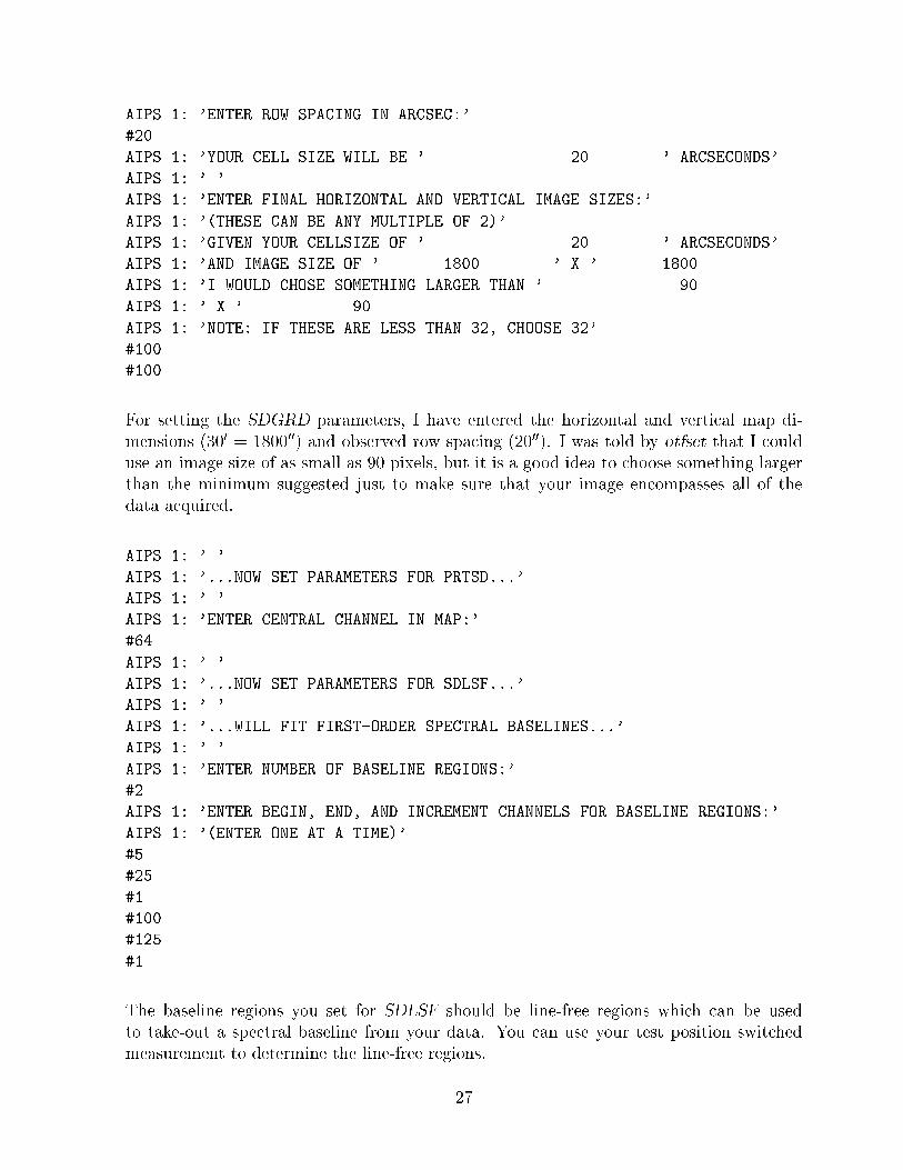
For setting the SDGRD parameters, I have entered the horizontal and vertical map di-mensions (300 = 180000) and observed row spacing (2000). I was told by otfset that I coulduse an image size of as small as 90 pixels, but it is a good idea to choose something largerthan the minimum suggested just to make sure that your image encompasses all of thedata acquired.

AIPS 1: ' '

AIPS 1: '...NOW SET PARAMETERS FOR PRTSD...'

AIPS 1: ' '

AIPS 1: 'ENTER CENTRAL CHANNEL IN MAP:'

#64

AIPS 1: ' '

AIPS 1: '...NOW SET PARAMETERS FOR SDLSF...'

AIPS 1: ' '

AIPS 1: '...WILL FIT FIRST-ORDER SPECTRAL BASELINES...'

AIPS 1: ' '

AIPS 1: 'ENTER NUMBER OF BASELINE REGIONS:'

#2

AIPS 1: 'ENTER BEGIN, END, AND INCREMENT CHANNELS FOR BASELINE REGIONS:'

AIPS 1: '(ENTER ONE AT A TIME)'

#5

#25

#1

#100

#125

#1

The baseline regions you set for SDLSF should be line-free regions which can be usedto take-out a spectral baseline from your data. You can use your test position switchedmeasurement to determine the line-free regions.

27

AIPS 1: 'ALL DONE SETTING OTF REDUCTION PARAMETERS'

Now that many of the more permanent OTF AIPS task parameters are set, we can runotfrun, which will ask a few more questions and actually process your map.

>otfrun

AIPS 1: 'SETTING OTF PROCEDURE PARAMETERS'

AIPS 1: ' '

AIPS 1: 'ENTER STARTING SEQUENCE NUMBER TO BE USED FOR ALL OUTPUT FILES:

'

AIPS 1: '(NOTE...SEQUENCE NUMBERS GREATER THAN OR EQUAL TO THIS VALUE'

AIPS 1: ' MUST BE UNIQUE)'

#1

This \sequence number" functions somewhat like the old VMS version numbers did andis a way of distinguishing AIPS data �les with the same name.

AIPS 1: ' '

AIPS 1: 'ENTER A UNIQUE NAME FOR AIPS OUTPUT FILES (IN SINGLE QUOTES):'

AIPS 1: '(SOME VARIATION ON THE OBJECT NAME WOULD BE A GOOD CHOICE)'

#'serpc18o'

AIPS 1: ' '

AIPS 1: 'YOUR DEFAULT AIPS OUTNAME WILL BE ' 'SERPC18O'

AIPS 1: ' '

AIPS 1: 'ENTER AIPS DISK NUMBER TO STORE DATA:'

#2

For the AIPS disk to store data, you should choose a number between 1 and 6. All of theoutput �les from the OTF AIPS tasks will reside on this disk, so it is a good idea to choosean AIPS disk with an ample amount of free space.

AIPS 1: ' '

AIPS 1: 'HOW MANY SDD FILES ARE YOU GOING TO READ?'

#2

I made two maps of this source and would like to process them both.

AIPS 1: ' '

AIPS 1: 'ENTER RAW DATA FILE NUMBER (IN SINGLE QUOTES):'

AIPS 1: '(NOTE...MUST BE A NUMBER LIKE 001)'

#'081'

28

AIPS 1: 'ARE YOU PROCESSING FILTERBANK OR MAC DATA?:'

AIPS 1: '(ENTER FB OR MAC IN SINGLE QUOTES)'

#'fb'

The �lter bank data for these maps is in data �les sdd.jgm 081 and sdd.jgm 082. If Iwere to process the millimeter autocorrelator data, it would look for the map data insdd hc.jgm 081 and sdd hc.jgm 082.

AIPS 1: 'IS THIS OFF-MADE DATA?:'

AIPS 1: '(I.E. HAVE YOU USED OTFMAKEOFFS?)'

AIPS 1: '(ENTER Y OR N IN SINGLE QUOTES)'

#'n'

OFF-made data is data that has been run through otfmakeo�s (see x5).

AIPS 1: ' '

AIPS 1: '...YOUR SDD FILE IS '

AIPS 1: 'OBSDAT:SDD.JGM_081 '

AIPS 1: '...YOUR GSDD FILE IS '

AIPS 1: 'OBSDAT:GSDD.JGM_081 '

AIPS 1: ' '

AIPS 1: 'HOW MANY SEPARATE BACKENDS ARE YOU GOING TO LOAD FROM THIS FILE?'

#1

I acquired this map in parallel mode, so I have two backends to process which I will need toput into two separate OTFUV �les. Each �le will have both polarizations concatenated foreach backend. At this point, I should explain the distinction between IF's and polarizations.An OTF measurement can consist of between 1 and 8 IF's. Each IF can be either anindependent frequency, the second polarization of a dual-polarization measurement, or anindependent beam element (for the 8-Beam receiver). Within AIPS, data samples aretagged with the IF number by using the \beam" random axis parameter. For example, anOTF map acquired in the �rst �lter bank IF will be IF number 01 and beam number 1,while an OTF map acquired in the �rst MAC IF will be IF number 11 and beam number11. This distinction between IF's within AIPS allows one to combine dual-polarizationor multiple-beam (8-Beam receiver) measurements into a single UV data �le. Tasks suchas SPFLG distinguish between IF's within the same data �le by reading each IF as an\autocorrelation pair". For example, data samples from IF number 18 are tagged asautocorrelation pair 18-18.

So for our parallel-mode �lter bank measurements, OTFUV will read IF's 01 and 02in one pass, and if you enter 03 for the polarization to load, will actually load IF's 03 and04 in one pass. In the following, I only loaded the �rst �lter bank set (IF's 01 and 02).

29

AIPS 1: ' '

AIPS 1: 'ENTER BACKEND NUMBER TO LOAD:'

AIPS 1: '(NOTE: ALL POLARIZATIONS ASSOCIATED WITH THIS BACKEND'

AIPS 1: 'WILL BE CONCATENATED)'

#1

AIPS 1: Resumes

AIPS 1: Task OTFUV has finished

Next, we load data from the second data �le in the same way as we did for the �rstdata �le.

AIPS 1: ' '

AIPS 1: 'ENTER RAW DATA FILE NUMBER (IN SINGLE QUOTES):'

AIPS 1: '(NOTE...MUST BE A NUMBER LIKE 001)'

#'082'

AIPS 1: 'ARE YOU PROCESSING FILTERBANK OR MAC DATA?:'

AIPS 1: '(ENTER FB OR MAC IN SINGLE QUOTES)'

#'fb'

AIPS 1: 'IS THIS OFF-MADE DATA?:'

AIPS 1: '(ENTER Y OR N)'

#'n'

AIPS 1: ' '

AIPS 1: '...YOUR SDD FILE IS '

AIPS 1: 'OBSDAT:SDD.JGM_082 '

AIPS 1: '...YOUR GSDD FILE IS '

AIPS 1: 'OBSDAT:GSDD.JGM_082 '

AIPS 1: ' '

AIPS 1: 'HOW MANY SEPARATE BACKENDS ARE YOU GOING TO LOAD FROM THIS FILE?'

#1

AIPS 1: ' '

AIPS 1: 'ENTER BACKEND NUMBER TO LOAD:'

AIPS 1: '(NOTE: ALL POLARIZATIONS ASSOCIATED WITH THIS BACKEND'

AIPS 1: 'WILL BE CONCATENATED)'

#1

AIPS 1: Resumes

AIPS 1: Task OTFUV has finished

At this point we have �nished loading the raw data into the OTFUV data �les. We cannow begin gridding the data.

AIPS 1: '...NOW RUNNING SDLSF ON SEQUENCE 1 ...'

AIPS 1: Resumes

AIPS 1: Task SDGRD has finished

30

AIPS 1: '...NOW RUNNING SDGRD ON SEQUENCE 1 ...'

AIPS 1: Resumes


AIPS 1: '...NOW RUNNING SDGRD TO CREATE A WEIGHTS IMAGE...'

AIPS 1: Resumes


Note that we have run the SDGRD task twice. The �rst pass through SDGRD was to gridthe data, while the second pass was to produce a weights image for this data cube whichcan be used in the WTSUM task (see x6.1.3).

AIPS 1: ' '

AIPS 1: 'ALL DONE PROCESSING MAP(S)'

AIPS 1: 'YOUR BASELINED CUBE(S) IS (ARE) ' 'SERPC18O '

AIPS 1: '.BASE;' 1 '-' 1

At this point, you have a processed map cube!

6.1.2 Step-By-Step Analysis

If after running otfset and otfrun you would like to run each AIPS task independently, youcan do so by using the tget verb in AIPS. Below I give a description of how to run eachtask.

OTFUV: Load your raw OTF data into AIPS for further processing using the task OT-FUV. Since otfset has already set many of the basic parameters for this procedure,including any data averaging selections you have made, you need only recall themfrom AIPS memory...

> tget otfuv

> bcount �rst scan to be included in map

> ecount last scan to be included in map

> inputs

You need only specify bcount and ecount if you need to exclude bad scans from yourmap (for example, you might have seen some bad data in your map while looking atit with Dataserve or Databrowse). If you are satis�ed with the input values, you canrun OTFUV with the \go" command...

> go

31

This will produce a UV data �le of your OTF map on the AIPS disk you speci�ed inotfset. NOTE: It is possible to average your 100 ms OTF data to the point whereyour sampling is greater than or equal to �

3D(1.5 times Nyquist) without sacri�cing

signal-to-noise or spatial resolution (Emerson, Jewell, & Mangum 1998). This is doneby specifying the yinc parameter in OTFUV. Please see the help and explain �les onOTFUV before using this method of data smoothing. Note also that we have notsuÆciently tested the e�ects of data smoothing on OTF data, so you should use thisfeature with caution.

PRTSD: The task PRTSD will print out useful information about your data which youcan use as a reference for further processing...

> tget prtsd

> getn uvdata�lenumber

> inputs

> go

SPFLG: The task SPFLG will allow you to edit your data using the AIPS TV display.Since SPFLG requires that your data be in \TB" order, you need to �rst run UVSRTon your UV data set...

> tget uvsrt


> sort 'TB'

> inputs

> go

By default, the output UV data �le from UVSRT will have the class name 'TBSRT'.It is this sorted UV data �le that one will edit in SPFLG and, if any editing is indeeddone, use in the subsequent analysis. The SPFLG parameters have been set suchthat your data will be time-smoothed within SPFLG to 0.5 seconds for editing anddisplay. Note that this is not a permanent smoothing of your data, but a necessitydue to the limited number of data points that SPFLG can process...

> tget spflg

> getn sorteduvdata�lenumber

> inputs

> go

32

The default settings will cause SPFLG to load the �rst IF (which is identi�ed in-ternally as autocorrelation baseline 01-01 in your UV data set) of your data set intothe TV display with channel number along the horizontal axis and time along thevertical axis. SPFLG has many options, which you might like to read about in theEXPLAIN �le for the task. Basic processing can be done by using any of the \clip"or \ ag" selections. If you have a dual-polarization data set, you can select and editthe second IF by using the \enter baseline" option (since there is only two \baselines"in your data set in this case, SPFLG will automatically choose the second one withthe \enter baseline" command). Note, though, that for strong (i.e. maser)sources, it is possible to mistake data samples with signal for bad samples.Be careful!

SDLSF: The task SDLSF will remove a least-squares-�t baseline from your raw (OTFUV)data. The output from SDLSF is a baseline-subtracted raw data �le. Since otfsethas already setup the default parameters for you, you need only recall these presetSDLSF parameters, tell SDLSF what UV data �le to process, review the inputs, andgo...

> tget sdlsf


> inputs

> go

...where uvdata�lenumber is the number of the UV data �le that you produced in theOTFUV step.

SDGRD: The task SDGRD will do a number of things to your OTF UV data set. Sinceyour UV data came into AIPS with no projection information, SDGRD will applythis information to your data set. The default projection (set by otfset) is the TAN(tangent) projection, which is the same projection in which the OTF data was ac-quired (for small �elds). SDGRD will then sort your UV data, followed by the actualgridding of the data. Since a Bessel function of the �rst kind of order 1 (J1(r)),divided by r, and multiplied by a Gaussian, is an appropriate gridding function forOTF data (see Mangum, Emerson, & Greisen 1999), otfset has preset the SDGRDgridding parameters so that the following gridding function is used...

J1�jrja

�jrja

� exp

24�

jrjb

!235

...where...

a = Nyquist sampling rate in pixels = 1.55

b ' half of the full width zero intensity for the primary beam = 2.52

33

The choice of the above function as the default convolution function is due to thefact that it gives the best representation of the response of the telescope beam to thesky distribution. Figures 7 and 8 show this and several other common convolutionfunctions with their associated Fourier transforms.

The output from SDGRD is a gridded/interpolated image cube. Since otfset hasalready setup the default parameters for you, you need only recall these preset SD-GRD parameters, tell SDGRD what UV data �le to process, review the inputs, andgo...

> tget sdgrd


> inputs

> go

...where uvdata�lenumber is either the number of the UV data �le that you producedin the OTFUV or the output UV data �le from your SDLSF step.

TVMOV: You can look at a \movie" of your baseline-subtracted cube channel imageplanes with the verb TVMOV. Do the following to look at a movie of your baseline-subtracted cube...

> getn baselinedcubenumber

> tvmov

Directions for changing the transfer function, color, frame rate, etc. will appear onyour screen.

6.1.3 Combining Multiple Maps

A common observing mode involves making many maps of a given �eld which are latercombined to build-up signal-to-noise. As described above, you can use OTFUV to loadeach polarization from each map data set into one UV data �le. If you have read andprocessed your maps and/or polarizations into AIPS individually and wish to combinethem as maps, use the task WTSUM. WTSUM requires four input maps/cubes; the twodata maps/cubes which are to be combined and their respective weights images. One canproduce a weights image for a given data cube by using SDGRD with REWEIGHT(1)= 3 (the 1/sigma**2 option) and BCHAN = ECHAN = 1 (the data weights are channelindependent). WTSUM will do a weighted-average of the two input maps/cubes. Theprocedures otfset and otfrun produce by default the necessary weights image you will needfor an analysis with WTSUM. You simply need to set the input parameters...

> task 'wtsum'

34

Figure 7: Representative convolution functions.

Figure 8: Representative Fourier transforms of convolution functions.

35

> indisk maplocation

> in2disk maplocation



> getn �rstgriddedcube

> get2n secondgriddedcube

> get3n �rstweightsimage

> get4n secondweightsimage

> doinver -1

> go

...where the doinver parameter will assure that we get the correct treatment of theweights images (see the AIPS help or explain �les for more information).

6.1.4 Spatial Smoothing

The AIPS task CONVL can be used to spatially smooth your gridded data. You shouldread the AIPS help or explain �le for this task for further information.

6.2 Continuum

In the following, I describe a general technique for processing spectral line OTF data takenat the 12 Meter. As a result of a great deal of e�ort by Eric Greisen, the reduction of OTFdata at the 12 Meter is done completely within the AIPS program. The diagram shownin Figure 9 gives a pictoral description of the processing steps one must follow to reduceOTF data.

Coming soon...

36

Figure 9: Continuum OTF data analysis ow chart.

37

6.3 More Extensive Processing

6.3.1 Integrated Intensity Images

XSUM: Integrated intensity images can be made using the task XSUM. Say you want tomake an integrated intensity image of channels 49 through 82 of your processed cube.You need to �rst make sure that the cube you want to make an integrated intensityimage of has velocity as its �rst axis. You can make such a cube using the TRANStask on your baseline-subtracted cube...

TRANS: This step is only necessary if you use the \old" processing route. You nowhave a channel map cube. You must now correct for any nonlinearities in yourspectral baselines. These nonlinearities will show up as declination stripes in yourmaps. Baseline removal in cubes is done using the IMLIN task. But, since IMLINexpects your data cube to have axes in an (velocity,RA,Dec) order, you need to �rstTRANSpose your cube to this axis order (transcode = '312'). Since otfset has alreadyset the TRANS task parameters for you, you need only recall these preset TRANSparameters, tell TRANS what �le to transpose, review the inputs, and go...

> tget trans


> inputs

> go

...where baselinedcubenumber is the number of the image cube �le that you producedin the SDGRD step.

...then run XSUM on this cube...

> task 'xsum'

> getn transposedcubenumber

> outn integratedintensityimagename

> outdisk indisk

> blc 49 0

> trc 82 0

> opco 'sum'

> go

38

...where baselinedcubenumber is the cube which resulted from the SDGRD task andintegratedintensityimagename is a name of your choosing. An example of an inte-grated intensity map taken from our sample Serpens data set is shown in the examplesfor the plotting tasks CNTR and GREYS given below.

NOTE: The units of this map should really be K*km/s. One can use the AIPS verbRESCALE to multiply this integrated intensity image by the channel width (0.845km/s in this case) and the verb PUTHEAD to insert the proper unit name (K*km/s)into the map header. I have done this for the example plots shown below.

6.3.2 Gaussian Fits

JMFIT: Gaussian �ts to individual channels can be made using the task JMFIT. Say yourintegrated intensity image has one main blob of emission to which you would like to�t a Gaussian.

> task 'jmfit'

> getn integratedintensityimagenumber

> tvall

> tvwin

> ngauss 1

> ctype 0

> domax 1

> dopos 1

> dowidth 1

> go

The TVALL and TVWIN steps will allow you to load the integrated intensity imageand determine the box (window) coordinates of the blob you want to Gaussian �t.

For information on other AIPS tasks that you might �nd usefull for processing yourOTF images, see the AIPS Cookbook.

39

6.3.3 Displaying Your Data

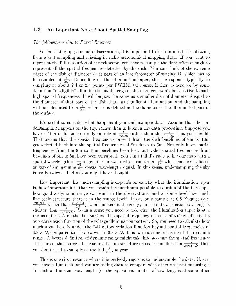
CNTR: Contour plots of individual maps can be made using the task CNTR. To makea contour plot of the integrated intensity map made above, I used the followinginputs...

> task 'cntr'


> clev 1

> levs 2,3,4,6,8

> go

Your plot will be attached to the integrated intensity image as a PL (plot) extension.To display it (either as hardcopy or on your workstation) you will need to use anyof the tasks LWPLA (for hardcopy output), TKPL (for a Tektronix display on yourAIPS Tek server), or TVPL (for a plot on your AIPS TV display). Figure 10 wasproduced using CNTR and LWPLA.

SERCTR IPOL SERPC18O.XSUM.1

PLot file version 1 created 07-SEP-1995 06:35:14

Peak flux = 8.2480E+00 K*KM/S Levs = 1.0000E+00 * ( 2.000, 3.000, 4.000, 6.000, 8.000)

DE

CL

INA

TIO

N (

B19

50)

RIGHT ASCENSION (B1950)18 27 45 30 15 00 26 45 30

01 20

15

10

05

00

Figure 10: Example output from the CNTR task.

40

GREYS: Greyscale and contour plots of individual maps can be made using the taskGREYS. To make a GREYS plot of the integrated intensity map made above, I usedthe following inputs...

> task 'greys'


> get2n integratedintensityimagenumber

> clev 1

> levs 2,3,4,5,6,8

> pixra 0 8

> dowedge 1

> go

As with CNTR, your plot will be attached to the integrated intensity image as a PL(plot) extension. To display it (either as hardcopy or on your workstation) you willneed to use any of the tasks LWPLA (for hardcopy output), TKPL (for a Tektronixdisplay on your AIPS Tek server), or TVPL (for a plot on your AIPS TV display).Figure 11 was produced using GREYS and LWPLA.

SERCTR IPOL SERPC18O.XSUM.1

Plot file version 2 created 07-SEP-1995 06:38:51

Grey scale flux range= 0.000 8.000 K*KM/S Peak contour flux = 8.2480E+00 K*KM/S Levs = 1.0000E+00 * ( 2.000, 3.000, 4.000, 6.000, 8.000)

DE

CL

INA

TIO

N (

B19

50)

RIGHT ASCENSION (B1950)18 27 45 30 15 00 26 45 30

01 20

15

10

05

00

0 2 4 6 8

Figure 11: Example output from the GREYS task.

41

KNTR: Contour plots of multichannel data can be made using the task KNTR. To makea KNTR plot of emission channels 60 through 63 from our processed Serpens dataset, I used the following inputs...

> task 'kntr'

> getn retransposedcubenumber

> clev 0.4

> levs -3,3,6,9,12

> blc 0 0 60

> trc 0 0 63

> go

As with CNTR, your plot will be attached to the integrated intensity image as a PL(plot) extension. To display it (either as hardcopy or on your workstation) you willneed to use any of the tasks LWPLA (for hardcopy output), TKPL (for a Tektronixdisplay on your AIPS Tek server), or TVPL (for a plot on your AIPS TV display).Figure 12 was produced using KNTR and LWPLA.

SERCTR 8.7 KM/S IPOL SERCTR.BASE.1


Peak flux = 4.7720E+00 K Levs = 4.0000E-01 * ( -3.00, 3.000, 6.000, 9.000, 12.00)

01 20

15

10

05

00

8.68 8.41

DE

CL

INA

TIO

N (

B19

50)

RIGHT ASCENSION (B1950)18 27 45 30 15 0026 45 30

01 20

15

10

05

00

8.14 7.86

Figure 12: Example output from the KNTR task.

42

PLCUB: Spectral plots of multichannel data can be made using the task PLCUB. To makea PLCUB plot of the spectra at the central 6 pixels processed (axis order must be(velocity,RA,Dec) Serpens data set, I used the following inputs...

> task 'plcub'


> pixra -0.5,3.5

> blc 0 31 31

> trc 0 33 33

> go

As with CNTR, your plot will be attached to the cube �le as a PL (plot) extension.To display it (either as hardcopy or on your workstation) you will need to use anyof the tasks LWPLA (for hardcopy output), TKPL (for a Tektronix display on yourAIPS Tek server), or TVPL (for a plot on your AIPS TV display). Figure 13 wasproduced using PLCUB and LWPLA.

DE

CL

INA

TIO

N (

B19

50)

RIGHT ASCENSION (B1950)18 27 25.0 24.5 24.0 23.5 23.0 22.5 22.0 21.5 21.0

01 13 00

12 45

30

15

SERCTR 8.1 KM/S IPOL SERCTR.BASE.2


K

Kilo VELO-LSR20 10 0

3.53.02.52.01.51.00.50.0

-0.5

Figure 13: Example output from the PLCUB task.

43

declination (b1950) 13 12 smm3 smm5 … (b1950) right ascension (b1950) 18 27 45 30 15 00 01 16 15...

Documents