decision trees: how to construct them and how to … decision tree tutorial by avi kak decision...
TRANSCRIPT

The Decision Tree Tutorial by Avi Kak
DECISION TREES: How to Construct
Them and How to Use Them for
Classifying New Data
Avinash Kak
Purdue University
August 28, 2017
8:59am
An RVL Tutorial Presentation
(First presented in Fall 2010; minor updates in August 2017)
c©2017 Avinash Kak, Purdue University
1
The Decision Tree Tutorial by Avi Kak
CONTENTS
Page
1 Introduction 3
2 Entropy 10
3 Conditional Entropy 15
4 Average Entropy 17
5 Using Class Entropy to Discover the Best Feature 19for Discriminating Between the Classes
6 Constructing a Decision Tree 25
7 Incorporating Numeric Features 38
8 The Python Module DecisionTree-3.4.3 50
9 The Perl Module Algorithm::DecisionTree-3.43 57
10 Bulk Classification of Test Data in CSV Files 64
11 Dealing with Large Dynamic-Range and 67Heavy-tailed Features
12 Testing the Quality of the Training Data 70
13 Decision Tree Introspection 76
14 Incorporating Bagging 84
15 Incorporating Boosting 92
16 Working with Randomized Decision Trees 102
17 Speeding Up DT Based Classification With Hash Tables 113
18 Constructing Regression Trees 120
19 Historical Antecedents of Decision Tree 125Classification in Purdue RVL
2

The Decision Tree Tutorial by Avi Kak
1. Introduction
• Let’s say your problem involves making a
decision based on N pieces of information.
Let’s further say that you can organize the
N pieces of information and the correspond-
ing decision as follows:
f_1 f_2 f_3 ...... f_N => DECISION---------------------------------------------------------------------------
val_1 val_2 val_3 ..... val_N => d1val_1 val_2 val_3 ..... val_N => d2val_1 val_2 val_3 ..... val_N => d1val_1 val_2 val_3 ..... val_N => d1val_1 val_2 val_3 ..... val_N => d3........
For convenience, we refer to each column
of the table as representing a feature f i
whose value goes into your decision making
process. Each row of the table represents
a set of values for all the features and the
corresponding decision.
3
The Decision Tree Tutorial by Avi Kak
• As to what specifically the features f i shownon the previous slide would be, that wouldobviously depend on your application. [In a
medical context, each feature f i could represent a laboratory
test on a patient, the value val i the result of the test, and
the decision d i the diagnosis. In drug discovery, each feature
f i could represent the name of an ingredient in the drug, the
value val i the proportion of that ingredient, and the decision
d i the effectiveness of the drug in a drug trial. In a Wall
Street sort of an application, each feature could represent a
criterion (such as the price-to-earnings ratio) for making a
buy/sell investment decision, and so on.]
• If the different rows of the training data,arranged in the form of a table shown onthe previous slide, capture adequately thestatistical variability of the feature valuesas they occur in the real world, you may beable to use a decision tree for automatingthe decision making process on any newdata. [As to what I mean by “capturing adequately the
statistical variability of feature values”, see Section 12 of this
tutorial.]
4

The Decision Tree Tutorial by Avi Kak
• Let’s say that your new data record for
which you need to make a decision looks
like:
new_val_1 new_val_2 new_val_2 .... new_val_N
the decision tree will spit out the best pos-
sible decision to make for this new data
record given the statistical distribution of
the feature values for all the decisions in
the training data supplied through the ta-
ble on Slide 3. The “quality” of this deci-
sion would obviously depend on the quality
of the training data, as explained in Section
12.
• This tutorial will demonstrate how the no-
tion of entropy can be used to construct a
decision tree in which the feature tests for
making a decision on a new data record are
organized optimally in the form of a tree of
decision nodes.
5
The Decision Tree Tutorial by Avi Kak
• In the decision tree that is constructed from
your training data, the feature test that is
selected for the root node causes maximal
disambiguation of the different possible de-
cisions for a new data record. [In terms of
information content as measured by entropy, the feature test
at the root would cause maximum reduction in the decision
entropy in going from all the training data taken together to
the data as partitioned by the feature test.]
• One then drops from the root node a set
of child nodes, one for each value of the
feature tested at the root node for the case
of symbolic features. For the case when a
numeric feature is tested at the root node,
one drops from the root node two child
nodes, one for the case when the value of
the feature tested at the root is less than
the decision threshold chosen at the root
and the other for the opposite case.
6
The Decision Tree Tutorial by Avi Kak
• Subsequently, at each child node, you posethe same question you posed at the rootnode when you selected the best featureto test at that node: Which feature test atthe child node in question would maximallydisambiguate the decisions for the train-ing data associated with the child node inquestion?
• In the rest of this Introduction, let’s seehow a decision-tree based classifier can beused by a computer vision system to au-tomatically figure out which features workthe best in order to distinguish between aset of objects. We assume that the visionsystem has been supplied with a very largenumber of elementary features (we couldrefer to these as the vocabulary of a com-puter vision system) and how to extractthem from images. But the vision systemhas NOT been told in advance as to whichof these elementary features are relevantto the objects.
7

The Decision Tree Tutorial by Avi Kak
• Here is how we could create such a self-
learning computer vision system:
– We show a number of different objects
to a sensor system consisting of cam-
eras, 3D vision sensors (such as the Mi-
crosoft Kinect sensor), and so on. Let’s
say these objects belong to M different
classes.
– For each object shown, all that we tell
the computer is its class label. We do
NOT tell the computer how to discrim-
inate between the objects belonging to
the different classes.
– We supply a large vocabulary of features
to the computer and also provide the
computer with tools to extract these
features from the sensory information
collected from each object.
8
The Decision Tree Tutorial by Avi Kak
– For image data, these features could
be color and texture attributes and the
presence or absence of shape primitives.
[For depth data, the features could be different types of
curvatures of the object surfaces and junctions formed by
the joins between the surfaces, etc.]
– The job given to the computer: From
the data thus collected, it must figure
out on its own how to best discrimi-
nate between the objects belonging to
the different classes. [That is, the computer
must learn on its own what features to use for discrimi-
nating between the classes and what features to ignore.]
• What we have described above constitutes
an exercise in a self-learning computer vi-
sion system.
• As mentioned in Section 19 of this tu-
torial, such a computer vision system was
successfully constructed and tested in my
laboratory at Purdue as a part of a Ph.D
thesis.
9
The Decision Tree Tutorial by Avi Kak
2. Entropy
• Entropy is a powerful tool that can be used
by a computer to determine on its own
own as to what features to use and how
to carve up the feature space for achieving
the best possible discrimination between
the classes. [You can think of each decision of a certain
type in the last column of the table on Slide 3 as defining a
class. If, in the context of computer vision, all the entries in
the last column boil down to one of “apple,” “orange,” and
“pear,” then your training data has a total of three classes.]
• What is entropy?
• If a random variable X can take N differ-
ent values, the ith value xi with probability
p(xi), we can associate the following en-
tropy with X:
H(X) = −
N∑
i=1
p(xi) log2 p(xi)
10
The Decision Tree Tutorial by Avi Kak
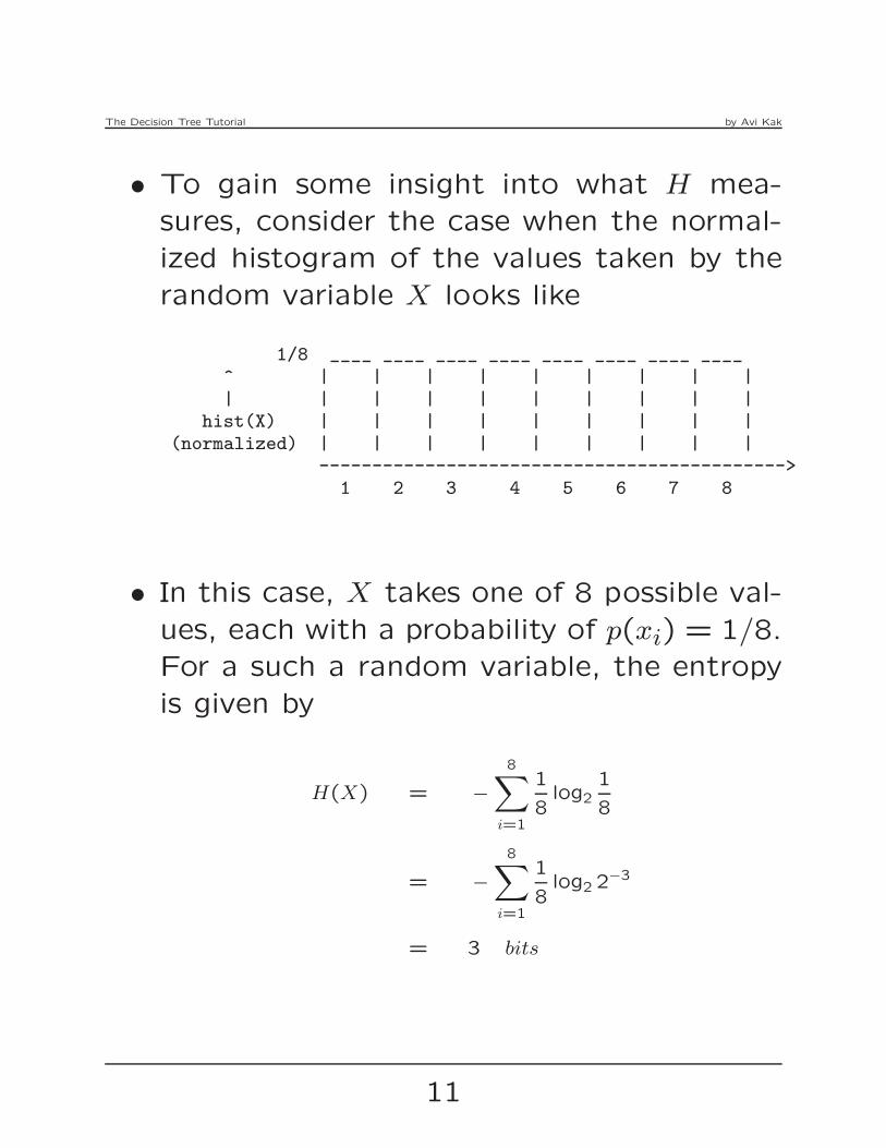
• To gain some insight into what H mea-
sures, consider the case when the normal-
ized histogram of the values taken by the
random variable X looks like
1/8 ____ ____ ____ ____ ____ ____ ____ ____^ | | | | | | | | || | | | | | | | | |
hist(X) | | | | | | | | |(normalized) | | | | | | | | |
-------------------------------------------->1 2 3 4 5 6 7 8
• In this case, X takes one of 8 possible val-
ues, each with a probability of p(xi) = 1/8.
For a such a random variable, the entropy
is given by
H(X) = −
8∑
i=1
1
8log2
1
8
= −
8∑
i=1
1
8log2 2
−3
= 3 bits
11
The Decision Tree Tutorial by Avi Kak
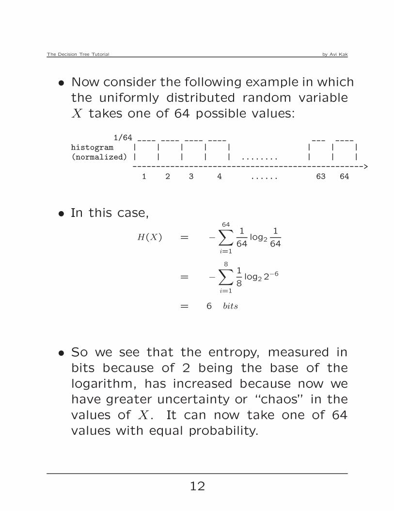
• Now consider the following example in which
the uniformly distributed random variable
X takes one of 64 possible values:
1/64 ____ ____ ____ ____ ___ ____histogram | | | | | | | |(normalized) | | | | | ........ | | |
------------------------------------------------->1 2 3 4 ...... 63 64
• In this case,
H(X) = −
64∑
i=1
1
64log2
1
64
= −
8∑
i=1
1
8log2 2
−6
= 6 bits
• So we see that the entropy, measured in
bits because of 2 being the base of the
logarithm, has increased because now we
have greater uncertainty or “chaos” in the
values of X. It can now take one of 64
values with equal probability.
12

The Decision Tree Tutorial by Avi Kak
• Let’s now consider an example at the other
end of the “chaos”: We will consider an Xthat is always known to take on a particular
value:
1.0 ___| || |
histogram | |(normalized) | |
| || 0 | 0 | 0 | 0 | | ........ | 0 | 0 |------------------------------------------------->
1 2 3 .. k ........ 63 64
• In this case, we obviously have
p(xi) = 1 xi = k
= 0 otherwise
• The entropy for such an X would be givenby:
H(X) = −
N∑
i=1
p(xi) log2 p(xi)
= − [p1 log2 p1 + ...pk log2 pk + ...+ pN log2 pN ]
13
The Decision Tree Tutorial by Avi Kak
= − 1× log2 1 bits
= 0 bits
where we use the fact that as p → 0+,
p log p → 0 in all of the terms of the sum-
mation except when i = k.
• So we see that the entropy becomes zero
when X has zero chaos.
• In general, the more nonuniform the
probability distribution for an entity, the
smaller the entropy associated with the
entity.
14
The Decision Tree Tutorial by Avi Kak
3. Conditional Entropy
• Given two interdependent random variables
X and Y , the conditional entropy H(Y |X)
measures how much entropy (chaos) re-
mains in Y if we already know the value of
the random variable X.
• In general,
H(Y |X) = H(X,Y ) − H(X)
The entropy contained in both variables
when taken together is H(X, Y ). The above
definition says that, if X and Y are interde-
pendent, and if we know X, we can reduce
our measure of chaos in Y by the chaos
that is attributable to X. [For independent X
and Y , one can easily show that H(X, Y ) = H(X) +H(Y ).]
15

The Decision Tree Tutorial by Avi Kak
• But what do we mean by knowing X in the
context of X and Y being interdependent?
Before we answer this question, let’s first
look at the formula for the joint entropy
H(X, Y ), which is given by
H(X,Y ) = −∑
i,j
p(
xi, yj)
log2 p(
xi, yj)
• When we say we know X, in general what
we mean is that we know that the variable
X has taken on a particular value. Let’s
say that X has taken on a specific value a.
The entropy associated with Y would now
be given by:
H(
Y∣
∣X=a)
= −∑
i
p(
yi∣
∣X=a)
× log2 p(
yi∣
∣X=a)
• The formula shown for H(Y |X) on the pre-
vious page is the average of H(
Y∣
∣
∣X = a)
over all possible instantiations a for X.
16
The Decision Tree Tutorial by Avi Kak
4. Average Entropies
• Given N independent random variables X1,
X2, . . .XN , we can associate an average
entropy with all N variables by
Hav =
N∑
1
H(Xi) × p(Xi)
• For another kind of an average, the condi-
tional entropy H(Y |X) is also an average,
in the sense that the right hand side shown
below is an average with respect to all of
the different ways the conditioning variable
can be instantiated:
H(
Y∣
∣X)
=∑
a
H(
Y∣
∣X=a)
× p(
X=a)
where H(
Y∣
∣X = a)
is given by the formula at
the bottom of the previous slide.
17

The Decision Tree Tutorial by Avi Kak
• To establish the claim made in the previous
bullet, note that
H
(
Y
∣
∣
∣X
)
=∑
a
H
(
Y
∣
∣
∣X=a
)
× p(X=a)
= −∑
a
{
∑
j
p
(
yj
∣
∣
∣X = a
)
log2 p
(
yj
∣
∣
∣X = a
)}
p(X = a)
= −∑
i
∑
j
p
(
yj
∣
∣
∣
xi
)
log2 p
(
yj
∣
∣
∣
xi
)
p(xi)
= −∑
i
∑
j
p(xi, yj)
p(xi)log2
p(xi, yj)
p(xi)p(xi)
= −∑
i
∑
j
p(xi, yj)
[
log2 p(xi, yj)− log2 p(xi)
]
= H(X,Y ) +∑
i
∑
j
p(xi, yj) log2 p(xi)
= H(X,Y ) +∑
i
p(xi) log2 p(xi)
= H(X,Y ) − H(X)
The 3rd expression is a rewrite of the 2nd
with a more compact notation. [In the 7th, we
note that we get a marginal probability when a joint probability
is summed with respect to its free variable.]
18

The Decision Tree Tutorial by Avi Kak
5. Using Class Entropy to Discover the
Best Feature for Discriminating Between
the Classes
• Consider the following question: Let us say
that we are given the measurement data as
described on Slides 3 and 4. Let the ex-
haustive set of features known to the com-
puter be {f1, f2, ....., fK}.
• Now the computer wants to know as to
which of these features is best in the sense
of being the most class discriminative.
• How does the computer do that?
19

The Decision Tree Tutorial by Avi Kak
• To discover the best feature, all that the
computer has to do is to compute the class
entropy as conditioned on each specific fea-
ture f separately as follows:
H(C|f) =∑
a
H(
C∣
∣
∣v(f) = a
)
× p(
v(f) = a)
where the notation v(f) = a means that
the value of feature f is some specific value
a. The computer selects that feature f for
which H(C|f) is the smallest value. [In
the formula shown above, the averaging carried out over the
values of the feature f is the same type of averaging as shown
at the bottom of Slide 17.] NOTATION: Note that
C is a random variable over the class labels. If your training
data mentions the following three classes: “apple,” “orange,”
and “pear,” then C as a random variable takes one of these
labels as its value.
• Let’s now focus on the calculation of the
right hand side in the equation shown above.
20

The Decision Tree Tutorial by Avi Kak
• The entropy in each term on the right hand
side in the equation shown on the previous
slide can be calculated by
H
(
C
∣
∣
∣
v(f) = a
)
= −∑
m
p
(
Cm
∣
∣
∣
v(f) = a
)
× log2 p
(
Cm
∣
∣
∣
v(f) = a
)
where Cm is the name of the mth class and
the summation is over all the classes.
• But how do we figure out p
(
Cm
∣
∣
∣
∣
v(f) = a
)
that is needed on the right hand side?
• We will next present two different ways for
calculating p
(
Cm
∣
∣
∣
∣
v(f) = a
)
. The first ap-
proach works if we can assume that the ob-
jects shown to the sensor system are drawn
uniformly from the different classes. If that
is not the case, one must use the second
approach.
21
The Decision Tree Tutorial by Avi Kak
• Our first approach for calculating p(Cm
∣
∣v(f)=
a) is count-based: Given M classes of objects
that we show to a sensor system, we pick objects
randomly from the population of all objects be-
longing to all classes. Say the sensor system is
allowed to measure K different kinds of features:
f1, f2, ...., fK. For each feature fk, the sensor sys-
tem keeps a count of the number of objects that
gave rise to the v(fk) = a value. Now we estimate
p(Cm
∣
∣v(f) = a) for any choice of f = fk simply by
counting off the number of objects from class Cm
that exhibited the v(fk) = a measurement.
• Our second approach for estimating p(
Cm
∣
∣v(f)=
a)
uses the Bayes’ Theorem:
p
(
Cm
∣
∣
∣v(f)=a
)
=
p
(
v(f)=a
∣
∣
∣Cm
)
× p(Cm)
p
(
v(f) = a
)
This formula also allows us to carry out
separate measurement experiments for ob-
jects belonging to different classes.
22
The Decision Tree Tutorial by Avi Kak
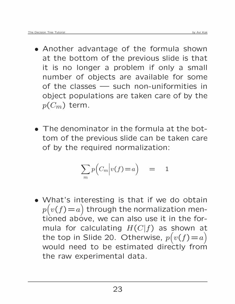
• Another advantage of the formula shown
at the bottom of the previous slide is that
it is no longer a problem if only a small
number of objects are available for some
of the classes — such non-uniformities in
object populations are taken care of by the
p(Cm) term.
• The denominator in the formula at the bot-
tom of the previous slide can be taken care
of by the required normalization:
∑
m
p(
Cm
∣
∣
∣v(f)=a
)
= 1
• What’s interesting is that if we do obtain
p(
v(f)=a)
through the normalization men-
tioned above, we can also use it in the for-
mula for calculating H(C|f) as shown at
the top in Slide 20. Otherwise, p(
v(f)=a)
would need to be estimated directly from
the raw experimental data.
23
The Decision Tree Tutorial by Avi Kak
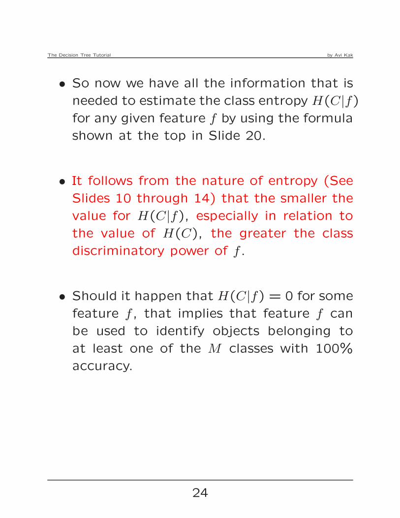
• So now we have all the information that is
needed to estimate the class entropy H(C|f)
for any given feature f by using the formula
shown at the top in Slide 20.
• It follows from the nature of entropy (See
Slides 10 through 14) that the smaller the
value for H(C|f), especially in relation to
the value of H(C), the greater the class
discriminatory power of f .
• Should it happen that H(C|f) = 0 for some
feature f , that implies that feature f can
be used to identify objects belonging to
at least one of the M classes with 100%
accuracy.
24
The Decision Tree Tutorial by Avi Kak
6. Constructing a Decision Tree
• Now that you know how to use the class
entropy to find the best feature that will
discriminate between the classes, we will
now extend this idea and show how you can
construct a decision tree. Subsequently
the tree may be used to classify future sam-
ples of data.
• But what is a decision tree?
• For those not familiar with decision tree
ideas, the traditional way to classify multi-
dimensional data is to start with a feature
space whose dimensionality is the same as
that of the data.
25
The Decision Tree Tutorial by Avi Kak
• In the traditional approach, each feature
in the space would correspond to the at-
tribute that each dimension of the data
measures. You then use the training data
to carve up the feature space into different
regions, each corresponding to a different
class. Subsequently, when you are trying to
classify a new data sample, you locate it in
the feature space and find the class label
of the region to which it belongs. One can
also give the data point the same class la-
bel as that of the nearest training sample.
(This is referred to as the nearest neighbor
classification.)
• A decision tree classifier works differently.
• When you construct a decision tree, you
select for the root node a feature test that
can be expected to maximally disambiguate
the class labels that could be associated
with the data you are trying to classify.
26

The Decision Tree Tutorial by Avi Kak
• You then attach to the root node a set of
child nodes, one for each value of the fea-
ture you chose at the root node. [This statement
is not entirely accurate. As you will see later, for the case of symbolic features, you create child nodes for only those
feature values (for the feature chosen at the root node) that reduce the class entropy in relation to the value of the class
entropy at the root.] Now at each child node you pose
the same question that you posed when
you found the best feature to use at the
root node: What feature at the child node
in question would maximally disambiguate
the class labels to be associated with a
given data vector assuming that the data
vector passed the root node on the branch
that corresponds to the child node in ques-
tion. The feature that is best at each node
is the one that causes the maximal reduc-
tion in class entropy at that node.
• Based on the discussion in the previous sec-
tion, you already know how to find the best
feature at the root node of a decision tree.
Now the question is: How we do construct
the rest of the decision tree?
27

The Decision Tree Tutorial by Avi Kak
• What we obviously need is a child node for
every possible value of the feature test that
was selected at the root node of the tree.
• Assume that the feature selected at the
root node is fj and that we are now at one
of the child nodes hanging from the root.
So the question now is how do we select
the best feature to use at the child node.
• The root node feature was selected as that
f which minimized H(C|f). With this choice,
we ended up with the feature fj at the
root. The feature to use at the child on the
branch v(fj) = aj will be selected as that
f 6= fj which minimizes H(
C∣
∣
∣v(fj)=aj, f)
.
[REMINDER: Whereas v(fj) stands for
the “value of feature fj,” the notation ajstands for a specific value taken by that
feature.]
28

The Decision Tree Tutorial by Avi Kak
• That is, for any feature f not previously
used at the root, we find the conditional
entropy (with respect to our choice for f) when we
are on the v(fj)=aj branch:
H
(
C
∣
∣
∣
f, v(fj) = aj
)
=
∑
b
H
(
C
∣
∣
∣
v(f)=b, v(fj)=aj
)
× p
(
v(f)=b, v(fj)=aj
)
Whichever feature f yields the smallest value
for the entropy mentioned on the left hand
side of the above equation will become the
feature test of choice at the branch in ques-
tion.
• Strictly speaking, the entropy formula shown
above for the calculation of average en-
tropy is not correct since it does not reflect
the fact that the probabilistic averaging on
the right hand side is only with respect to
the values taken on by the feature f .
29
The Decision Tree Tutorial by Avi Kak
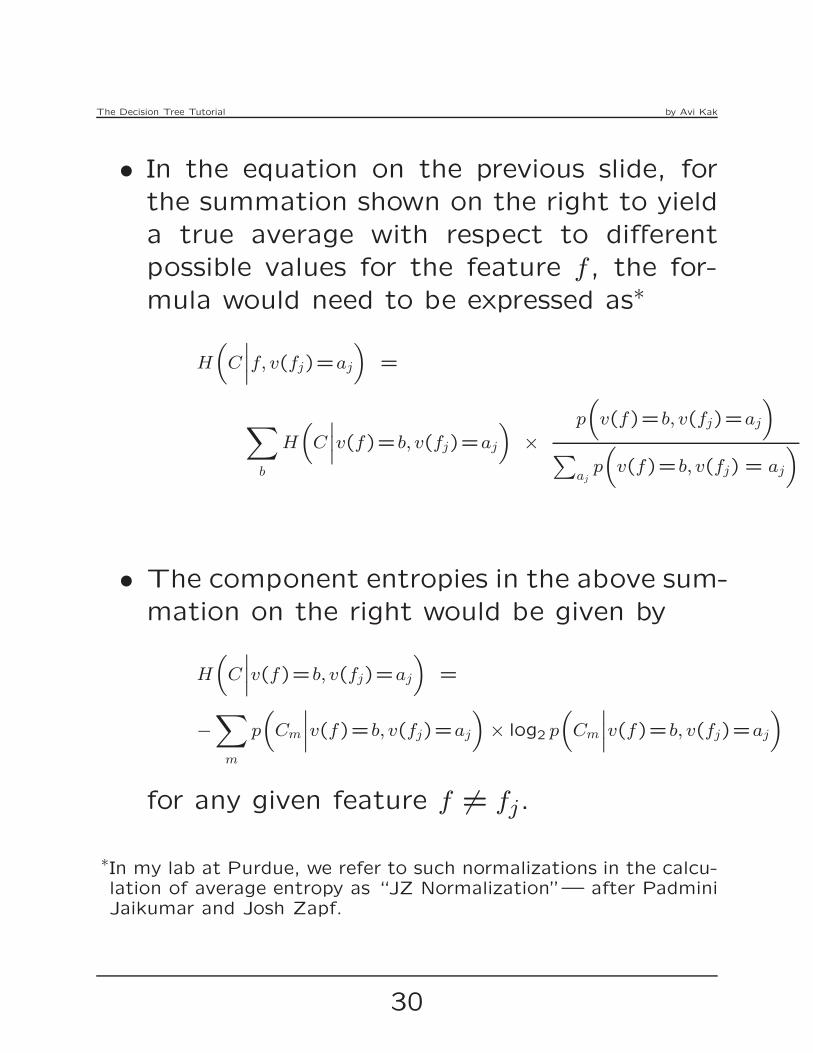
• In the equation on the previous slide, for
the summation shown on the right to yield
a true average with respect to different
possible values for the feature f , the for-
mula would need to be expressed as∗
H
(
C
∣
∣
∣f, v(fj)=aj
)
=
∑
b
H
(
C
∣
∣
∣v(f)=b, v(fj)=aj
)
×
p
(
v(f)=b, v(fj)=aj
)
∑
ajp
(
v(f)=b, v(fj) = aj
)
• The component entropies in the above sum-
mation on the right would be given by
H
(
C
∣
∣
∣v(f)=b, v(fj)=aj
)
=
−∑
m
p
(
Cm
∣
∣
∣
v(f)=b, v(fj)=aj
)
× log2 p
(
Cm
∣
∣
∣
v(f)=b, v(fj)=aj
)
for any given feature f 6= fj.
∗In my lab at Purdue, we refer to such normalizations in the calcu-lation of average entropy as “JZ Normalization”— after PadminiJaikumar and Josh Zapf.
30
The Decision Tree Tutorial by Avi Kak
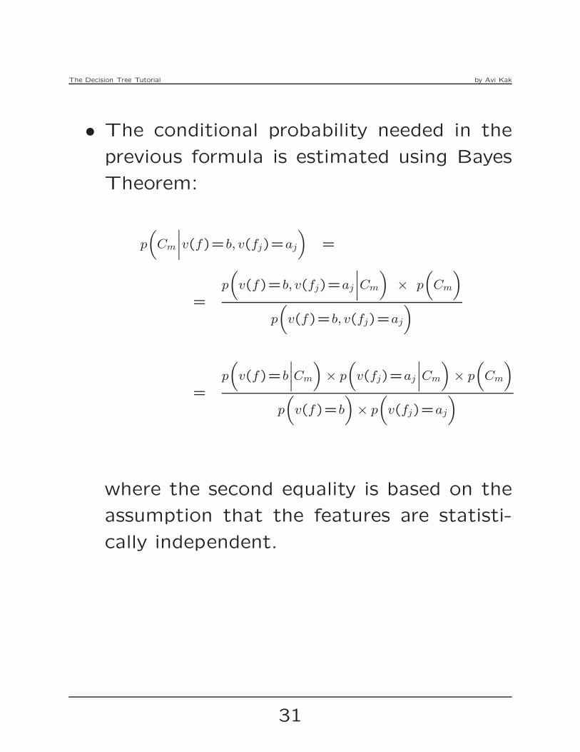
• The conditional probability needed in the
previous formula is estimated using Bayes
Theorem:
p
(
Cm
∣
∣
∣
v(f)=b, v(fj)=aj
)
=
=
p
(
v(f)=b, v(fj)=aj
∣
∣
∣
Cm
)
× p
(
Cm
)
p
(
v(f)=b, v(fj)=aj
)
=
p
(
v(f)=b
∣
∣
∣Cm
)
× p
(
v(fj)=aj
∣
∣
∣Cm
)
× p
(
Cm
)
p
(
v(f)=b
)
× p
(
v(fj)=aj
)
where the second equality is based on the
assumption that the features are statisti-
cally independent.
31
The Decision Tree Tutorial by Avi Kak
Feature Tested at This Nodef
Feature Tested at Root
f j
f = 1j f = 2
j
Feature Tested at This Nodef k l
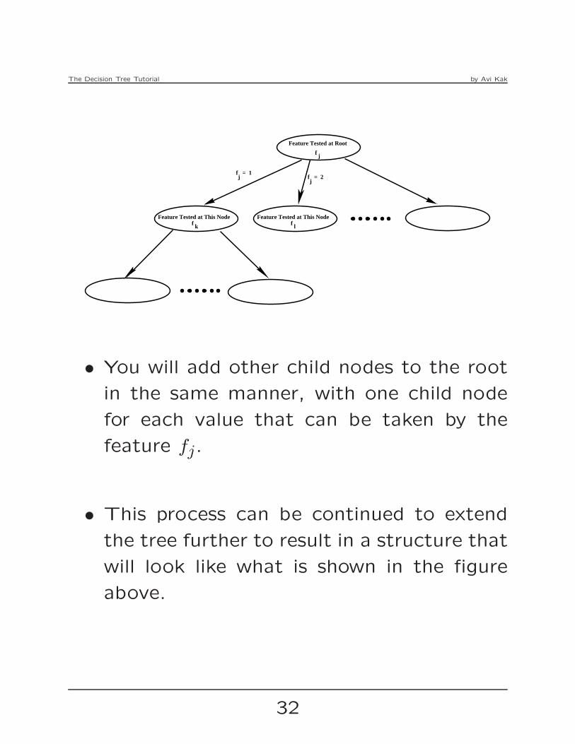
• You will add other child nodes to the root
in the same manner, with one child node
for each value that can be taken by the
feature fj.
• This process can be continued to extend
the tree further to result in a structure that
will look like what is shown in the figure
above.
32

The Decision Tree Tutorial by Avi Kak
• Now we will address the very important is-
sue of the stopping rule for growing the
tree. That is, when does a node get a fea-
ture test so that it can be split further and
when does it not?
• A node is assigned the entropy that re-
sulted in its creation. For example, the
root gets the entropy H(C) computed from
the class priors.
• The children of the root are assigned the
entropy H(C∣
∣
∣fj) that resulted in their cre-
ation.
• A child node of the root that is on the
branch v(fj)=aj gets its own feature test
(and is split further) if and only if we can
find a feature fk such that H(
C∣
∣fk, v(fj)=aj
)
is less than the entropy H(C∣
∣
∣fj) inherited
by the child from the root.
33
The Decision Tree Tutorial by Avi Kak
• If the condition H
(
C
∣
∣
∣f, v(fj) = aj
)
< H
(
C
∣
∣
∣fj)
)
cannot be satisfied at the child node on the
branch v(fj) = aj of the root for any fea-
ture f 6= fj, the child node remains without
a feature test and becomes a leaf node of
the decision tree.
• Another reason for a node to become a
leaf node is that we have used up all the
features along that branch up to that node.
• That brings us to the last important is-
sue related to the construction of a de-
cision tree: associating class probabilities
with each node of the tree.
• As to why we need to associate class prob-
abilities with the nodes in the decision tree,
let us say we are given for classification a
new data vector consisting of features and
their corresponding values.
34
The Decision Tree Tutorial by Avi Kak
• For the classification of the new data vec-
tor mentioned above, we will first subject
this data vector to the feature test at the
root. We will then take the branch that
corresponds to the value in the data vec-
tor for the root feature.
• Next, we will subject the data vector to
the feature test at the child node on that
branch. We will continue this process until
we have used up all the feature values in
the data vector. That should put us at one
of the nodes, possibly a leaf node.
• Now we wish to know what the residual
class probabilities are at that node. These
class probabilities will represent our classi-
fication of the new data vector.
35

The Decision Tree Tutorial by Avi Kak
• If the feature tests along a path to a node
in the tree are v(fj)=aj, v(fk)=bk, . . ., we
will associate the following class probability
with the node:
p
(
Cm
∣
∣
∣
∣
v(fj)=aj, v(fk)=bk, . . .
)
for m = 1,2, . . . ,M where M is the number
of classes.
• The above probability may be estimated
with Bayes Theorem:
p(
Cm
∣
∣
∣v(fj)=aj, v(fk)=bk, . . .
)
=
p(
v(fj)=aj, v(fk)=bk, . . .∣
∣
∣Cm
)
× p(
Cm
)
p(
v(fj)=aj, v(fk)=bk, . . .)
36

The Decision Tree Tutorial by Avi Kak
• If we again use the notion of statistical
independence between the features both
when they are considered on their own and
when considered conditioned on a given
class, we can write:
p
(
v(fj)=aj, v(fk)=bk, . . .
)
=∏
f on branch
p
(
v(f)=value
)
p
(
v(fj)=aj, v(fk) = bk, . . .
∣
∣
∣Cm
)
=∏
f on branch
p
(
v(f) = value
∣
∣
∣Cm
)
37

The Decision Tree Tutorial by Avi Kak
7. Incorporating Numeric Features
• A feature is numeric if it can take any
floating-point value from a continuum of
values. The sort of reasoning we have de-
scribed so far for choosing the best feature
at a node and constructing a decision tree
cannot be applied directly to the case of
numeric features.
• However, numeric features lend themselves
to recursive partitioning that eventually re-
sults in the same sort of a decision tree you
have seen so far.
• When we talked about symbolic features in
Section 5, we calculated the class entropy
with respect to a feature by constructing a
probabilistic average of the class entropies
with respect to knowing each value sepa-
rately for the feature.
38

The Decision Tree Tutorial by Avi Kak
• Let’s say f is a numeric feature. For a
numeric feature, a better approach consists
of calculating the class entropy vis-a-vis a
decision threshold on the feature values:
H
(
C
∣
∣
∣
vth(f) = θ
)
= H
(
C
∣
∣
∣
v(f) ≤ θ
)
× p
(
v(f) ≤ θ
)
+
H
(
C
∣
∣
∣
v(f) > θ
)
× p
(
v(f) > θ
)
where vth(f) = θ means that we have set
the decision threshold for the values of the
feature f at θ for the purpose of parti-
tioning the data into parts, one for which
v(f) ≤ θ and the other for which v(f) > θ.
• The left side in the equation shown above
is the average entropy for the two parts
considered separately on the right hand side.
The threshold for which this average en-
tropy is the minimum is the best threshold
to use for the numeric feature f .
39

The Decision Tree Tutorial by Avi Kak
• To illustrate the usefulness of minimizing
this average entropy for discovering the best
threshold, consider the case when we have
only two classes, one for which all values
of f are less than θ and the other for which
all values of f are greater than θ. For this
case, the left hand side above would be
zero.
• The components entropies on the right hand
side in the previous equation can be calcu-
lated by
H
(
C
∣
∣
∣
v(f) ≤ θ
)
= −∑
m
p
(
Cm
∣
∣
∣
v(f) ≤ θ
)
× log2 p
(
Cm
∣
∣
∣
v(f) ≤ θ
)
and
H
(
C
∣
∣
∣v(f) > θ
)
= −∑
m
p
(
Cm
∣
∣
∣v(f) > θ
)
× log2 p
(
Cm
∣
∣
∣v(f) > θ
)
40

The Decision Tree Tutorial by Avi Kak
• We can estimate p(
Cm
∣
∣v(f)≤θ)
and p(
Cm
∣
∣v(f)>
θ)
by using the Bayes’ Theorem:
p
(
Cm
∣
∣
∣v(f)≤θ
)
=
p
(
v(f)≤θ
∣
∣
∣
Cm
)
× p(Cm)
p
(
v(f) ≤ θ
)
and
p
(
Cm
∣
∣
∣v(f)>θ
)
=
p
(
v(f)>θ
∣
∣
∣
Cm
)
× p(Cm)
p
(
v(f) > θ
)
The various terms on the right sides in the
two equations shown above can be esti-
mated directly from the training data.
• However, in practice, you are better off us-
ing the normalization shown on the next
page for estimating the denominator in the
equations shown above.
41

The Decision Tree Tutorial by Avi Kak
• Although the denominator in the equations
on the previous slide can be estimated di-
rectly from the training data, you are likely
to achieve superior results if you calculate
this denominator directly from (or, at least,
adjust its calculated value with) the follow-
ing normalization constraint on the proba-
bilities on the left:
∑
m
p(
Cm
∣
∣
∣v(f) ≤ θ
)
= 1
and
∑
m
p(
Cm
∣
∣
∣v(f) > θ
)
= 1
• Now we are all set to use this partitioning
logic to choose the best feature for the
root node of our decision tree. We proceed
as explained on the next slide.
42
The Decision Tree Tutorial by Avi Kak
• Given a set of numeric features and a train-
ing data file, we seek that numeric feature
for which the average entropy over the two
parts created by the thresholding partition
is the least.
• For each numeric feature, we scan through
all possible partitioning points (these would
obviously be the sampling points over the
interval corresponding to the values taken
by that feature), and we choose that par-
titioning point which minimizes the aver-
age entropy of the two parts. We consider
this partitioning point as the best decision
threshold to use vis-a-vis that feature.
• Given a set of numeric features, their as-
sociated best decision thresholds, and the
corresponding average entropies over the
partitions obtained, we select for our best
feature that feature that has the least av-
erage entropy associated with it at its best
decision threshold.
43

The Decision Tree Tutorial by Avi Kak
• After finding the best feature for the root
node in the manner described above, we
can drop two branches from it, one for the
training samples for which v(f) ≤ θ and the
other for the samples for which v(f) > θ as
shown in the figure below:
Feature Tested at Root
f
f )v( f )v(
j
j j> θ<= θ
• The argument stated above can obviously
be extended to a mixture of numeric and
symbolic features as explained on the next
slide.
44

The Decision Tree Tutorial by Avi Kak
• Given a mixture or symbolic and numeric
features, we associate with each symbolic
feature the best possible entropy calculated
in the manner explained in Section 5. And,
we associate with each numeric feature the
best entropy that corresponds to the best
threshold choice for that feature. Given all
the features and their associated best class
entropies, we choose that feature for the
root node of our decision tree for which
the class entropy is the minimum.
• Now that you know how to construct the
root node for the case when you have just
numeric features or a mixture of numeric
and symbolic features, the next question is
how to branch out from the root node.
• If the best feature selected for the root
node is symbolic, we proceed in the same
way as described in Section 5 in order to
grow the tree to the next level.
45

The Decision Tree Tutorial by Avi Kak
• On the other hand, if the best feature f
selected at the root node is numeric and
the best decision threshold for the feature
is θ, we must obviously construct two child
nodes at the root, one for which v(f) ≤ θ
and the other for which v(f) > θ.
• To extend the tree further, we now select
the best features to use at the child nodes
of the root. Let’s assume for a moment
that the best feature chosen for a child
node also turns out to be numeric.
• Let’s say we used the numeric feature fj,
along with its decision threshold θj, at the
root and that the choice of the best feature
to use at the left child turns out to be fkand that its best decision threshold is θk.
46

The Decision Tree Tutorial by Avi Kak
• The choice (fk, θk) at the left child of the
root must be the best possible among all
possible features and all possible thresholds
for those features so that following average
entropy is minimized:
H
(
C
∣
∣
∣v(fj) ≤ θj, v(fk) ≤ θk
)
× p
(
v(fj) ≤ θj, v(fk) ≤ θk
)
+
H
(
C
∣
∣
∣
v(fj) ≤ θj, v(fk) > θk
)
× p
(
v(fj) ≤ θk, v(fk) > θk
)
• For the purpose of our explanations, we
assume that the left child at a node with a
numeric test feature always corresponds to
the “less than or equal to the threshold”
case and the right child to the “greater
than the threshold” case.
47
The Decision Tree Tutorial by Avi Kak
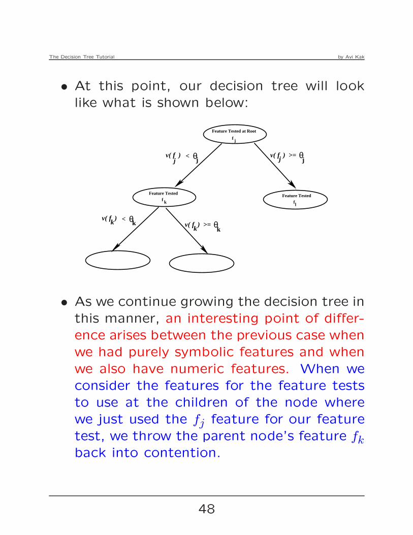
• At this point, our decision tree will look
like what is shown below:
Feature Tested Feature Tested
Feature Tested at Root
f
v( f < )
f f
v( f ) >= v( f < )
j
jv( f ) >=
j
k l
kk
θ θ
θθ
j j
kk
• As we continue growing the decision tree in
this manner, an interesting point of differ-
ence arises between the previous case when
we had purely symbolic features and when
we also have numeric features. When we
consider the features for the feature tests
to use at the children of the node where
we just used the fj feature for our feature
test, we throw the parent node’s feature fkback into contention.
48
The Decision Tree Tutorial by Avi Kak
• In general, this difference between the deci-
sion trees for the purely symbolic case and
the decision trees needed when you must
also deal with numeric features is more il-
lusory than real. That is because when
considering the root node feature fl at the
third-level nodes in the tree, the values of
fl will be limited to the interval [vmin(fl), θl)
in the left children of the root and to the
interval [θl, vmax(fl)) in the right children
of the root. Testing for whether the value
of the feature fl is in, say, the interval
[v(fmin(fl), θl) is not the same feature test
as testing for whether this value is in the
interval [vmin(fl), vmax(fl)).
• Once we arrive at a child node, we carry
out at the child node the same reasoning
that we carried out at the root for the se-
lection of the best feature at the child node
and to then grow the tree accordingly.
49

The Decision Tree Tutorial by Avi Kak
8. The Python Module
DecisionTree-3.4.3
NOTE: Versions prior to 2.0 could only handle symbolic train-
ing data. Versions 2.0 and higher can handle both symbolic and
numeric training data.
• Version 2.0 was a major re-write of the
module for incorporating numeric features.
• Version 2.1 was a cleaned up version of v.
2.0. Version 2.2 introduced the functional-
ity to evaluate the quality of training data.
The latest version is 3.4.3. To download
Version 3.4.3:
https://engineering.purdue.edu/kak/distDT/DecisionTree-3.4.3.html
Click on the active link shown above to navi-
gate directly to the API of this software pack-
age.
50

The Decision Tree Tutorial by Avi Kak
• The module makes the following two as-sumptions about the training data in a ‘.csv’
file: that the first column (meaning thecolumn with index 0) contains a unique in-
teger identifier for each data record, andthat the first row contains the names to
be used for the features.
• Shown below is a typical call to the con-structor of the module:
training_datafile = "stage3cancer.csv"
dt = DecisionTree.DecisionTree(training_datafile = training_datafile,csv_class_column_index = 2,csv_columns_for_features = [3,4,5,6,7,8],entropy_threshold = 0.01,max_depth_desired = 3,symbolic_to_numeric_cardinality_threshold = 10,csv_cleanup_needed = 1,
)
In this call to the DecisionTree constructor,the option csv class column index is used to tell
the module that the class label is in the col-umn indexed 2 (meaning the third column)of the ‘.csv’ training data file.
51

The Decision Tree Tutorial by Avi Kak
• The constructor option csv columns for features
is used to tell the module that the columns
indexed 3 through 8 are to be used as fea-
tures.
• To explain the role of the constructor op-
tion symbolic to numeric cardinality threshold in
the call shown on the previous slide, note
that the module can treat those numeric
looking features symbolically if the differ-
ent numerical values taken by the feature
are small in number. In the call shown, if
a numeric feature takes 10 or fewer unique
values, it will be treated like a symbolic
feature.
• If the module can treat certain numeric
features symbolically, you might ask as to
what happens if the value for such a feature
in a test sample is not exactly the same as
one of the values in the training data.
52
The Decision Tree Tutorial by Avi Kak
• When a numeric feature is treated symbol-
ically, a value in a test sample is “snapped”
to the closest value in the training data.
• No matter whether you construct a de-
cision tree from purely symbolic data, or
purely numeric data, or a mixture of the
two, the two constructor parameters that
determine the number of nodes in the deci-
sion are entropy threshold and max depth desired.
More on these on the next slide.
• As for the role of entropy threshold, recall
that a child node is created only if the dif-
ference between the entropy at the current
node and the child node exceeds a thresh-
old. This parameter sets that threshold.
• Regarding the parameter max depth desired, note
that the tree is grown in a depth-first man-
ner to the maximum depth set by this pa-rameter.
53

The Decision Tree Tutorial by Avi Kak
• The option csv cleanup needed is important for
extracting data from “messy” CSV files.
That is, CSV files that use double-quoted
strings for either the field names or the field
values and that allow for commas to be
used inside the double-quoted strings.
• After the call to the constructor, the fol-lowing three methods must be called toinitialize the probabilities:
dt.get_training_data()dt.calculate_first_order_probabilities_for_numeric_features()dt.calculate_class_priors()
• The tree itself is constructed and, if so de-sired, displayed by the following calls:
root_node = dt.construct_decision_tree_classifier()root_node.display_decision_tree(" ")
where the “white-space” string supplied as
the argument to the display method is used
to offset the display of the child nodes in
relation to the display of the parent nodes.
54

The Decision Tree Tutorial by Avi Kak
• After you have constructed a decision tree,
it is time classify a test sample.
• Here is an example of the syntax used for atest sample and the call you need to maketo classify it:
test_sample = [’g2 = 4.2’,’grade = 2.3’,’gleason = 4’,’eet = 1.7’,’age = 55.0’,’ploidy = diploid’]
classification = dt.classify(root_node, test_sample)
• The classification returned by the call to
classify() as shown on the previous slide
is a dictionary whose keys are the class
names and whose values are the classifica-
tion probabilities associated with the classes.
• For further information, see the various ex-
ample scripts in the Examples subdirectory
of the module.
55

The Decision Tree Tutorial by Avi Kak
• The module also allows you to generate
your own synthetic symbolic and numeric
data files for experimenting with decision
trees.
• For large test datasets, see the next section
for the demonstration scripts that show
you how you can classify all your data records
in a CSV file in one go.
• See the web page at
https://engineering.purdue.edu/kak/distDT/DecisionTree-3.4.3.html
for a full description of the API of this
Python module.
56

The Decision Tree Tutorial by Avi Kak
9. The Perl Module
Algorithm::DecisionTree-3.43
NOTE: Versions 2.0 and higher of this module can handle simulta-
neously the numeric and the symbolic features. Even for the purely
symbolic case, you are likely to get superior results with the latest
version of the module than with the older versions.
• The goal of this section is to introduce
the reader to some of the more impor-
tant functions in my Perl module Algo-
rithm::DecisionTree that can be down-
loaded by clicking at the link shown below:
http://search.cpan.org/ avikak/Algorithm-DecisionTree-3.43/lib/Algorithm/DecisionTree.pm
Please read the documentation at the CPAN
site for the API of this software package. [If
clicking on the link shown above does not work you, you can
also just do a Google search on “Algorithm::DecisionTree”
and go to Version 3.43 when you get to the CPAN page for
the module.]
57

The Decision Tree Tutorial by Avi Kak
• To use the Perl module, you first need to
construct an instance of the Algorithm::DecisionTree
class as shown below:
my $training_datafile = "stage3cancer.csv";
my $dt = Algorithm::DecisionTree->new(training_datafile => $training_datafile,csv_class_column_index => 2,csv_columns_for_features => [3,4,5,6,7,8],entropy_threshold => 0.01,max_depth_desired => 8,symbolic_to_numeric_cardinality_threshold => 10,csv_cleanup_needed => 1,
);
• The constructor option csv class column index
informs the module as to which column of
your CSV file contains the class labels for
the data records. THE COLUMN INDEX-
ING IS ZERO BASED. The constructor
option csv columns for features specifies which
columns are to be used for feature values.
The first row of the CSV file must specify
the names of the features. See examples
of CSV files in the Examples subdirectory of
the module.
58
The Decision Tree Tutorial by Avi Kak
• The option symbolic to numeric cardinality threshold
in the constructor is also important. For
the example shown above, if an ostensibly
numeric feature takes on only 10 or fewer
different values in your training data file,
it will be treated like a symbolic features.
The option entropy threshold determines the
granularity with which the entropies are
sampled for the purpose of calculating en-
tropy gain with a particular choice of de-
cision threshold for a numeric feature or a
feature value for a symbolic feature.
• The option csv cleanup needed is important for
extracting data from “messy” CSV files.
That is, CSV files that use double-quoted
strings for either the field names or the field
values and that allow for commas to be
used inside the double-quoted strings.
59
The Decision Tree Tutorial by Avi Kak
• After you have constructed an instance of
the DecisionTree module, you read in the
training data file and initialize the proba-
bility cache by calling:
$dt->get_training_data();$dt->calculate_first_order_probabilities();$dt->calculate_class_priors();
• Now you are ready to construct a decision
tree for your training data by calling:
$root_node = $dt->construct_decision_tree_classifier();
where $root node is an instance of the DTNode
class that is also defined in the module file.
• With that, you are ready to start classifying
new data samples — as I show on the next
slide.
60
The Decision Tree Tutorial by Avi Kak
• Let’s say that your data record looks like:
my @test_sample = qw / g2=4.2
grade=2.3
gleason=4
eet=1.7age=55.0
ploidy=diploid /;
you can classify it by calling:
my $classification = $dt->classify($root_node, \@test_sample);
• The call to classify() returns a reference
to a hash whose keys are the class names
and the values the associated classification
probabilities. This hash also includes an-
other key-value pair for the solution path
from the root node to the leaf node at
which the final classification was carried
out.
61

The Decision Tree Tutorial by Avi Kak
• The module also allows you to generate
your own training datasets for experiment-
ing with decision trees classifiers. For that,
the module file contains the following classes:
(1) TrainingDataGeneratorNumeric, and
(2) TrainingDataGeneratorSymbolic
• The class TrainingDataGeneratorNumeric outputs
a CSV training data file for experimenting
with numeric features.
• The numeric values are generated using
a multivariate Gaussian distribution whose
mean and covariance are specified in a pa-
rameter file. See the file param numeric.txt
in the Examples directory for an example of
such a parameter file. Note that the di-
mensionality of the data is inferred from
the information you place in the parameter
file.
62
The Decision Tree Tutorial by Avi Kak
• The class TrainingDataGeneratorSymbolic gener-
ates synthetic training data for the purely
symbolic case. It also places its output
in a ‘.csv’ file. The relative frequencies
of the different possible values for the fea-
tures is controlled by the biasing informa-
tion you place in a parameter file. See
param symbolic.txt for an example of such a
file.
• See the web page at
http://search.cpan.org/~avikak/Algorithm-DecisionTree-3.43/
for a full description of the API of this Perl
module.
• Additionally, for large test datasets, see
Section 10 of this Tutorial for the demon-
stration scripts in the Perl module that show
you how you can classify all your data records
in a CSV file in one go.
63

The Decision Tree Tutorial by Avi Kak
10. Bulk Classification of All Test Data
Records in a CSV File
• For large test datasets, you would obvi-
ously want to process an entire file of test
data records in one go.
• The Examples directory of both the Perl and
the Python versions of the module include
demonstration scripts that show you how
you can classify all your data records in one
fell swoop if the records are in a CSV file.
• For the case of Perl, see the following scripts
in the Examples directory of the module for
bulk classification of data records:
classify test data in a file.pl
64

The Decision Tree Tutorial by Avi Kak
• And for the case of Python, check out the
following script in the Examples directory for
doing the same things:
classify test data in a file.py
• All scripts mentioned on this section re-
quire three command-line arguments, the
first argument names the training datafile,
the second the test datafile, and the third
the file in which the classification results
will be deposited.
• The other examples directories, ExamplesBagging,
ExamplesBoosting, and ExamplesRandomizedTrees,
also contain scripts that illustrate how to
carry out bulk classification of data records
when you wish to take advantage of bag-
ging, boosting, or tree randomization. In
their respective directories, these scripts
are named:
65

The Decision Tree Tutorial by Avi Kak
bagging_for_bulk_classification.plboosting_for_bulk_classification.plclassify_database_records.pl
bagging_for_bulk_classification.pyboosting_for_bulk_classification.pyclassify_database_records.py
66

The Decision Tree Tutorial by Avi Kak
11. Dealing with Large Dynamic-Range
and Heavy-tailed Features
• For the purpose of estimating the probabil-
ities, it is necessary to sample the range of
values taken on by a numerical feature. For
features with “nice” statistical properties,
this sampling interval is set to the median
of the differences between the successive
feature values in the training data. (Obvi-
ously, as you would expect, you first sort all
the values for a feature before computing
the successive differences.) This logic will
not work for the sort of a feature described
below.
• Consider a feature whose values are heavy-
tailed, and, at the same time, the values
span a million to one range.
67

The Decision Tree Tutorial by Avi Kak
• What I mean by heavy-tailed is that rare
values can occur with significant probabili-
ties. It could happen that most of the val-
ues for such a feature are clustered at one
of the two ends of the range. At the same
time, there may exist a significant number
of values near the end of the range that is
less populated.
• Typically, features related to human eco-
nomic activities — such as wealth, incomes,
etc. — are of this type.
• With the median-based method of setting
the sampling interval as described on the
previous slide, you could end up with a
sampling interval that is much too small.
That could potentially result in millions of
sampling points for the feature if you are
not careful.
68
The Decision Tree Tutorial by Avi Kak
• Beginning with Version 2.22 of the Perl
module and Version 2.2.4 of the Python
module, you have two options for dealing
with such features. You can choose to go
with the default behavior of the module,
which is to sample the value range for such
a feature over a maximum of 500 points.
• Or, you can supply an additional option
to the constructor that sets a user-defined
value for the number of points to use. The
name of the option is number of histogram bins.
The following script
construct_dt_for_heavytailed.pl
in the “examples” directory shows an ex-
ample of how to call the constructor of the
module with the number of histogram bins
option.
69
The Decision Tree Tutorial by Avi Kak
12. Testing the Quality of the TrainingData
• Even if you have a great algorithm for con-structing a decision tree, its ability to cor-rectly classify a new data sample would de-pend ultimately on the quality of the train-ing data.
• Here are the four most important reasonsfor why a given training data file may beof poor quality: (1) Insufficient numberof data samples to adequately capture thestatistical distributions of the feature val-ues as they occur in the real world; (2) Thedistributions of the feature values in thetraining file not reflecting the distributionas it occurs in the real world; (3) The num-ber of the training samples for the differentclasses not being in proportion to the real-world prior probabilities of the classes; and(4) The features not being statistically in-dependent.
70

The Decision Tree Tutorial by Avi Kak
• A quick way to evaluate the quality of your
training data is to run an N-fold cross-
validation test on the data. This test di-
vides all of the training data into N parts,
with N − 1 parts used for training a deci-
sion tree and one part used for testing the
ability of the tree to classify correctly. This
selection of N−1 parts for training and one
part for testing is carried out in all of the N
different possible ways. Typically, N = 10.
• You can run a 10-fold cross-validation test
on your training data with version 2.2 or
higher of the Python Decision Tree mod-
ule and version 2.1 or higher of the Perl
version of the same.
• The next slide presents a word of caution
in using the output of a cross-validation to
either trust or not trust your training data
file.
71
The Decision Tree Tutorial by Avi Kak
• Strictly speaking, a cross-validation testis statistically meaningful only if thetraining data does NOT suffer fromany of the four shortcomings I men-tioned at the beginning of this section.[The real purpose of a cross-validation test is to
estimate the Bayes classification error — meaning
the classification error that can be attributed to the
overlap between the class probability distributions in
the feature space.]
• Therefore, one must bear in mind the fol-lowing when interpreting the results of across-validation test: If the cross-validationtest says that your training data is of poorquality, then there is no point in using a de-cision tree constructed with this data forclassifying future data samples. On theother hand, if the test says that your datais of good quality, your tree may still be apoor classifier of the future data sampleson account of the four data shortcomingsmentioned at the beginning of this section.
72

The Decision Tree Tutorial by Avi Kak
• Both the Perl and the Python Decision-
Tree modules contain a special subclass
EvalTrainingData that is derived from the
main DecisionTree class. The purpose of
this subclass is to run a 10-fold cross-validation
test on the training data file you specify.
• The code fragment shown below illustrateshow you invoke the testing function of theEvalTrainingData class in the Python ver-sion of the module:
training_datafile = "training3.csv"eval_data = DecisionTree.EvalTrainingData(
training_datafile = training_datafile,csv_class_column_index = 1,csv_columns_for_features = [2,3],entropy_threshold = 0.01,max_depth_desired = 3,symbolic_to_numeric_cardinality_threshold = 10,csv_cleanup_needed = 1,
)eval_data.get_training_data()eval_data.evaluate_training_data()
In this case, we obviously want to evaluate
the quality of the training data in the file
training3.csv.
73

The Decision Tree Tutorial by Avi Kak
• The last statement in the code shown on
the previous slide prints out a Confusion
Matrix and the value of Training Data Qual-
ity Index on a scale of 0 to 100, with 100
designating perfect training data. The Con-
fusion Matrix shows how the different classes
were misidentified in the 10-fold cross-validation
test.
• The syntax for invoking the data testing
functionality in Perl is the same:
my $training_datafile = "training3.csv";
my $eval_data = EvalTrainingData->new(
training_datafile => $training_datafile,csv_class_column_index => 1,
csv_columns_for_features => [2,3],
entropy_threshold => 0.01,
max_depth_desired => 3,
symbolic_to_numeric_cardinality_threshold => 10,
csv_cleanup_needed => 1,);
$eval_data->get_training_data();
$eval_data->evaluate_training_data()
74
The Decision Tree Tutorial by Avi Kak
• This testing functionality can also be used
to find the best values one should use for
the constructor parameters entropy threshold,
max depth desired, and symbolic to numeric
cardinality threshold.
• The following two scripts in the Examples
directory of the Python version of the mod-
ule:
evaluate_training_data1.pyevaluate_training_data2.py
and the following two in the Examples di-
rectory of the Perl version
evaluate_training_data1.plevaluate_training_data2.pl
illustrate the use of the EvalTrainingData
class for testing the quality of your data.
75
The Decision Tree Tutorial by Avi Kak
13. Decision Tree Introspection
• Starting with Version 2.3.1 of the Python
module and with Version 2.30 of the Perl
module, you can ask the DTIntrospection
class of the modules to explain the clas-
sification decisions made at the different
nodes of the decision tree.
• Perhaps the most important bit of infor-
mation you are likely to seek through DT
introspection is the list of the training sam-
ples that fall directly in the portion of the
feature space that is assigned to a node.
• However, note that, when training samples
are non-uniformly distributed in the under-
lying feature space, it is possible for a node
76

The Decision Tree Tutorial by Avi Kak
to exist even when there are no training
samples in the portion of the feature space
assigned to the node. [That is because the de-
cision tree is constructed from the probability den-
sities estimated from the training data. When the
training samples are non-uniformly distributed, it is
entirely possible for the estimated probability densi-
ties to be non-zero in a small region around a point
even when there are no training samples specifically
in that region. (After you have created a statisti-
cal model for, say, the height distribution of people
in a community, the model may return a non-zero
probability for the height values in a small inter-
val even if the community does not include a single
individual whose height falls in that interval.)]
• That a decision-tree node can exist even
where there are no training samples in that
portion of the feature space that belongs
to the node is an important indicator of
the generalization abilities of a decision-
tree-based classifier.
77
The Decision Tree Tutorial by Avi Kak
• In light of the explanation provided above,
before the DTIntrospection class supplies
any answers at all, it asks you to accept
the fact that features can take on non-
zero probabilities at a point in the feature
space even though there are zero training
samples at that point (or in a small re-
gion around that point). If you do not ac-
cept this rudimentary fact, the introspec-
tion class will not yield any answers (since
you are not going to believe the answers
anyway).
• The point made above implies that the
path leading to a node in the decision tree
may test a feature for a certain value or
threshold despite the fact that the portion
of the feature space assigned to that node
is devoid of any training data.
78
The Decision Tree Tutorial by Avi Kak
• See the following three scripts in the Examples
directory of Version 2.3.2 or higher of the
Python module for how to carry out DT
introspection:
introspection_in_a_loop_interactive.pyintrospection_show_training_samples_at_all_nodes_direct_influence.py
introspection_show_training_samples_to_nodes_influence_propagation.py
and the following three scripts in the Examples
directory of Version 2.31 or higher of the
Perl module
introspection_in_a_loop_interactive.pl
introspection_show_training_samples_at_all_nodes_direct_influence.pl
introspection_show_training_samples_to_nodes_influence_propagation.pl
• In both cases, the first script places you
in an interactive session in which you will
first be asked for the node number you are
interested in.
79
The Decision Tree Tutorial by Avi Kak
• Subsequently, you will be asked for whether
or not you are interested in specific ques-
tions that the introspection can provide an-
swers for.
• The second of the three scripts listed on
the previous slide descends down the deci-
sion tree and shows for each node the train-
ing samples that fall directly in the portion
of the feature space assigned to that node.
• The last of the three script listed on the
previous slide shows for each training sam-
ple how it affects the decision-tree nodes
either directly or indirectly through the gen-
eralization achieved by the probabilistic mod-
eling of the data.
80
The Decision Tree Tutorial by Avi Kak
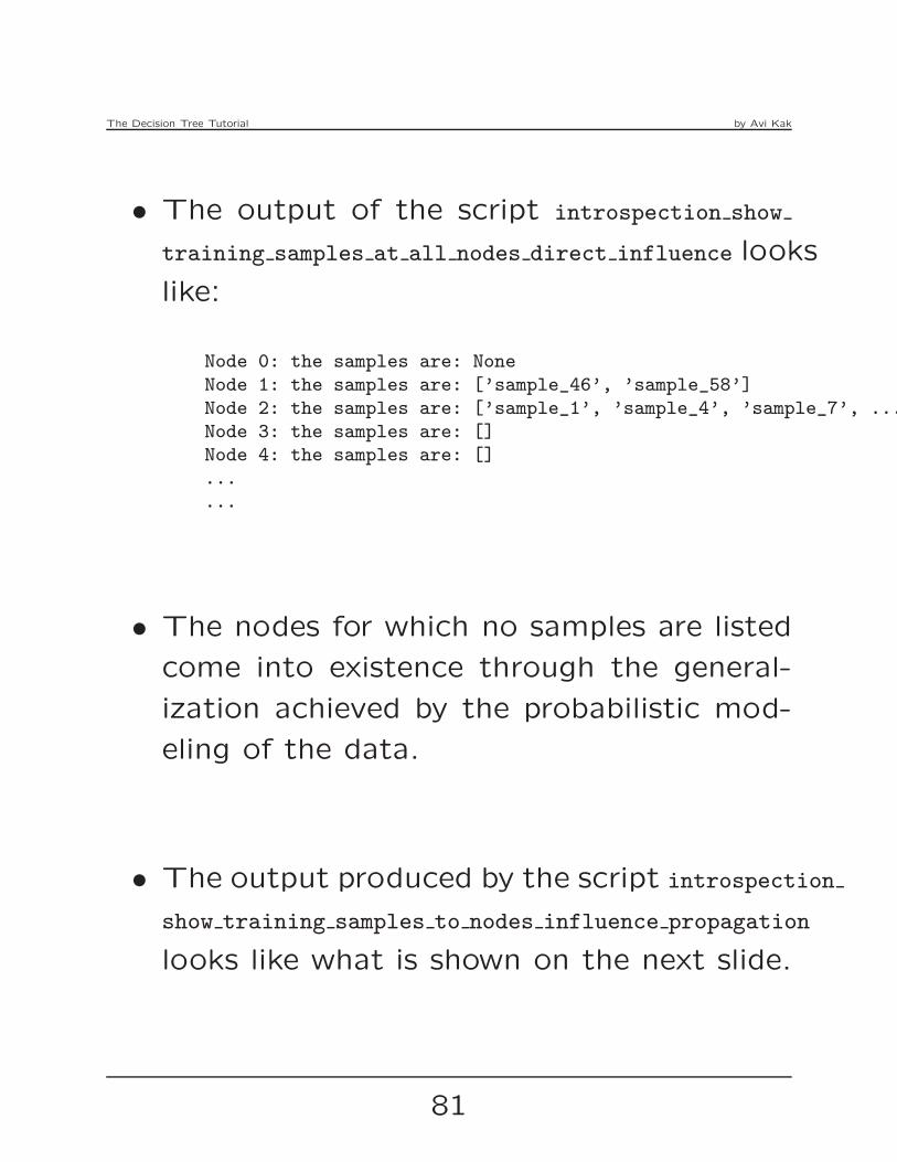
• The output of the script introspection show
training samples at all nodes direct influence looks
like:
Node 0: the samples are: None
Node 1: the samples are: [’sample_46’, ’sample_58’]
Node 2: the samples are: [’sample_1’, ’sample_4’, ’sample_7’, .....]
Node 3: the samples are: []Node 4: the samples are: []
...
...
• The nodes for which no samples are listed
come into existence through the general-
ization achieved by the probabilistic mod-
eling of the data.
• The output produced by the script introspection
show training samples to nodes influence propagation
looks like what is shown on the next slide.
81

The Decision Tree Tutorial by Avi Kak
sample_1:nodes affected directly: [2, 5, 19, 23]nodes affected through probabilistic generalization:
2=> [3, 4, 25]25=> [26]
5=> [6]6=> [7, 13]
7=> [8, 11]8=> [9, 10]11=> [12]
13=> [14, 18]14=> [15, 16]
16=> [17]19=> [20]
20=> [21, 22]23=> [24]
sample_4:nodes affected directly: [2, 5, 6, 7, 11]nodes affected through probabilistic generalization:
2=> [3, 4, 25]25=> [26]
5=> [19]19=> [20, 23]
20=> [21, 22]23=> [24]
6=> [13]13=> [14, 18]
14=> [15, 16]16=> [17]
7=> [8]8=> [9, 10]
11=> [12]
...
...
...
82
The Decision Tree Tutorial by Avi Kak
• For each training sample, the display on
the previous slide first presents the list of
nodes that are directly affected by the sam-
ple. A node is affected directly by a sam-
ple if the latter falls in the portion of the
feature space that belongs to the former.
Subsequently, for each training sample, the
display shows a subtree of the nodes that
are affected indirectly by the sample through
the generalization achieved by the proba-
bilistic modeling of the data. In general,
a node is affected indirectly by a sample if
it is a descendant of another node that is
affected directly.
• In the on-line documentation associated with
the Perl and the Python modules, the sec-
tion titled “The Introspection API” lists
the methods you can invoke in your own
code for carrying out DT introspection.
83

The Decision Tree Tutorial by Avi Kak
14. Incorporating Bagging
• Starting with Version 3.0 of the Python
DecisionTree module and Version 3.0 of the
Perl version of the same you can now carry
out decision-tree based classification with
bagging.
• Bagging means randomly extracting smaller
datasets (we refer to them as bags of data)
from the main training dataset and con-
structing a separate decision tree for each
bag. Subsequently, given a test sample,
you can classify it with each decision tree
and base your final classification on, say,
the majority vote from all the decision trees.
84

The Decision Tree Tutorial by Avi Kak
• (1) If your original training dataset is suffi-
ciently large; (2) you have done a good job
of catching in it all of the significant sta-
tistical variations for the different classes,
and (3) assuming that no single feature is
too dominant with regard to inter-class dis-
criminations, bagging has the potential to
reduce classification noise and bias.
• In both the Python and the Perl versions of
the DecisionTree module, bagging is imple-
mented through the DecisionTreeWithBagging
class.
• When you construct an instance of this
class, you specify the number of bags through
the constructor parameter how many bags and
the extent of overlap in the data in the bags
through the parameter bag overlap fraction,
as shown on the next slide.
85
The Decision Tree Tutorial by Avi Kak
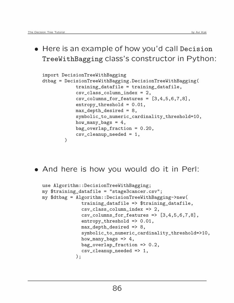
• Here is an example of how you’d call Decision
TreeWithBagging class’s constructor in Python:
import DecisionTreeWithBaggingdtbag = DecisionTreeWithBagging.DecisionTreeWithBagging(
training_datafile = training_datafile,csv_class_column_index = 2,csv_columns_for_features = [3,4,5,6,7,8],entropy_threshold = 0.01,max_depth_desired = 8,symbolic_to_numeric_cardinality_threshold=10,how_many_bags = 4,bag_overlap_fraction = 0.20,csv_cleanup_needed = 1,
)
• And here is how you would do it in Perl:
use Algorithm::DecisionTreeWithBagging;my $training_datafile = "stage3cancer.csv";my $dtbag = Algorithm::DecisionTreeWithBagging->new(
training_datafile => $training_datafile,csv_class_column_index => 2,csv_columns_for_features => [3,4,5,6,7,8],entropy_threshold => 0.01,max_depth_desired => 8,symbolic_to_numeric_cardinality_threshold=>10,how_many_bags => 4,bag_overlap_fraction => 0.2,csv_cleanup_needed => 1,
);
86
The Decision Tree Tutorial by Avi Kak
• As mentioned previously, the constructor
parameters how many bags and bag overlap fraction
determine how bagging is carried vis-a-vis
your training dataset.
• As implied by the name of the parameter,
the number of bags is set by how many bags.
Initially, the entire training dataset is ran-
domized and divided into how many bags non-
overlapping partitions. Subsequently, we
expand each such partition by a fraction
equal to bag overlap fraction by drawing
samples randomly from the other bags. For
example, if how many bags is set to 4 and
bag overlap fraction set to 0.2, we first di-
vide the training dataset (after it is ran-
domized) into 4 non-overlapping partitions
and then add additional samples drawn from
the other partitions to each partition.
87
The Decision Tree Tutorial by Avi Kak
• To illustrate, let’s say that the initial non-
overlapping partitioning of the training data
yields 100 training samples in each bag.
With bag overlap fraction set to 0.2, we
next add to each bag 20 additional train-
ing samples that are drawn randomly from
the other three bags.
• After you have constructed an instance of
the DecisionTreeWithBagging class, you can
call the following methods of this class for
the bagging based decision-tree classifica-
tion:get training data for bagging(): This method reads
your training datafile, randomizes it, and thenpartitions it into the specified number of bags.Subsequently, if the constructor parameter bagoverlap fraction is some positive fraction, it addsto each bag a number of additional samplesdrawn at random from the other bags. As tohow many additional samples are added to eachbag, suppose the parameter bag overlap fractionis set to 0.2, the size of each bag will grow by20% with the samples drawn from the otherbags.
88
The Decision Tree Tutorial by Avi Kak
show training data in bags(): Shows for each bagthe name-tags of the training data samples inthat bag.
calculate first order probabilities(): Calls on theappropriate methods of the main DecisionTreeclass to estimate the first-order probabilities fromthe samples in each bag.
calculate class priors(): Calls on the appropriatemethod of the main DecisionTree class to esti-mate the class priors for the data classes foundin each bag.
construct decision trees for bags(): Calls on theappropriate method of the main DecisionTreeclass to construct a decision tree from the train-ing data in each bag.
display decision trees for bags(): Display separatelythe decision tree for each bag.
classify with bagging( test sample ): Calls on theappropriate methods of the main DecisionTreeclass to classify the argument test sample.
display classification results for each bag(): Displaysseparately the classification decision made byeach the decision tree constructed for each bag.
89

The Decision Tree Tutorial by Avi Kak
get majority vote classification(): Using major-ity voting, this method aggregates the classifi-cation decisions made by the individual decisiontrees into a single decision.
See the example scripts in the directory Exam-plesBagging for how to call these methods forclassifying individual samples and for bulk clas-sification when you place all your test samplesin a single file.
• The ExamplesBagging subdirectory in the main
installation directory of the modules con-
tains the following scripts that illustrate
how you can incorporate bagging in your
decision tree based classification:
bagging_for_classifying_one_test_sample.py
bagging_for_bulk_classification.py
The same subdirectory in the Perl version
of the module contains the following scripts:
bagging_for_classifying_one_test_sample.pl
bagging_for_bulk_classification.pl
90

The Decision Tree Tutorial by Avi Kak
• As the name of the script implies, the first
Perl or Python script named on the pre-
vious slide shows how to call the different
methods of the DecisionTreeWithBagging class
for classifying a single test sample.
• When you are classifying a single test sam-
ple, as in the first of the two scripts named
on the previous slide, you can also see how
each bag is classifying the test sample. You
can, for example, display the training data
used in each bag, the decision tree con-
structed for each bag, etc.
• The second script named on the previous
slide is for the case when you place all
of the test samples in a single file. The
demonstration script displays for each test
sample a single aggregate classification de-
cision that is obtained through majority vot-
ing by all the decision trees.
91
The Decision Tree Tutorial by Avi Kak
15. Incorporating Boosting
• Starting with Version 3.2.0 of the Python
DecisionTree module and Version 3.20 of
the Perl version of the same, you can now
use boosting for decision-tree based classi-
fication.
• In both cases, the module includes a new
class called BoostedDecisionTree that makes
it easy to incorporate boosting in a decision-
tree classifier. [NOTE: Boosting does not
always result in superior classification per-
formance. Ordinarily, the theoretical guar-
antees provided by boosting apply only to
the case of binary classification. Addition-
ally, your training dataset must capture all
of the significant statistical variations in
the classes represented therein.]
92
The Decision Tree Tutorial by Avi Kak
• If you are not familiar with boosting, you
may want to first browse through my tu-
torial “AdaBoost for Learning Binary and
Multiclass Discriminations” that is avail-
able at:
https://engineering.purdue.edu/kak/Tutorials/AdaBoost.pdf
Boosting for designing classifiers owes its
origins to the now celebrated paper “A Decision-
Theoretic Generalization of On-Line Learn-
ing and an Application to Boosting” by
Yoav Freund and Robert Schapire that ap-
peared in 1995 in the Proceedings of the
2nd European Conf. on Computational
Learning Theory.
• A boosted decision-tree classifier consists
of a cascade of decision trees in which each
decision tree is constructed with samples
that are mostly those that are misclassified
by the previous decision tree.
93

The Decision Tree Tutorial by Avi Kak
• You specify a probability distribution over
the training dataset for selecting samples
for training each decision tree in the cas-
cade. At the beginning, the distribution is
uniform over all of the samples.
• Subsequently, this probability distribution
changes according to the misclassifications
by each tree in the cascade: if a sample
is misclassified by a given tree in the cas-
cade, the probability of its being selected
for training the next tree increases signifi-
cantly.
• You also associate a trust factor with each
decision tree depending on its power to
classify correctly all of the training data
samples.
94

The Decision Tree Tutorial by Avi Kak
• After a cascade of decision trees is con-
structed in this manner, you construct a
final classifier that calculates the class label
for a test data sample by taking into ac-
count the classification decisions made by
each individual tree in the cascade, the de-
cisions being weighted by the trust factors
associated with the individual classifiers.
• Here is an example of how you’d call the
constructor of the BoostedDecisionTree class
in Python:
import BoostedDecisionTreetraining_datafile = "training6.csv"
boosted = BoostedDecisionTree.BoostedDecisionTree(training_datafile = training_datafile,csv_class_column_index = 1,csv_columns_for_features = [2,3],entropy_threshold = 0.01,max_depth_desired = 8,symbolic_to_numeric_cardinality_threshold = 10,how_many_stages = 10,csv_cleanup_needed = 1,
)
95
The Decision Tree Tutorial by Avi Kak
• And here is an example of how you’d call
the constructor of the BoostedDecisionTree
class in Perl:
use Algorithm::BoostedDecisionTree;my $training_datafile = "training6.csv";my $boosted = Algorithm::BoostedDecisionTree->new(
training_datafile => $training_datafile,csv_class_column_index => 1,csv_columns_for_features => [2,3],entropy_threshold => 0.01,max_depth_desired => 8,symbolic_to_numeric_cardinality_threshold=>10,how_many_stages => 4,csv_cleanup_needed => 1,
);
• In both constructor calls shown above, note
the parameter how many stages. This pa-
rameter controls how many stages will be
used in the boosted decision tree classifier.
As mentioned earlier, a separate decision
tree is constructed for each stage of boost-
ing using a set of training samples drawn
randomly through a probability distribution
maintained over the entire training dataset.
96

The Decision Tree Tutorial by Avi Kak
• After you have constructed an instance of
the BoostedDecisionTree class, you can call
the following methods of this class for con-
structing the full cascade of decision trees
and for boosted decision-tree classification
of your test data:
• get training data for base tree(): In this methodname, the string base tree refers to the firsttree of the cascade. This is the tree for whichthe training samples are drawn assuming a uni-form distribution over the entire dataset. Thismethod reads your training datafile, creates thedata structures from the data ingested for con-structing the base decision tree.
show training data for base tree(): Shows the train-ing data samples and some relevant propertiesof the features used in the training dataset.
calculate first order probabilities and class priors():This method calls on the appropriate methodsof the main DecisionTree class to estimate thefirst-order probabilities and the class priors.
97
The Decision Tree Tutorial by Avi Kak
construct base decision tree(): This method callson the appropriate method of the main DecisionTreeclass to construct the base decision tree.
display base decision tree(): As you would guess,this method displays the base decision tree.
construct cascade of trees(): Uses the AdaBoostalgorithm (described in the AdaBoost tutorialmentioned at the beginning of this section) toconstruct a cascade of decision trees. As men-tioned earlier, the training samples for each treein the cascade are drawn using a probability dis-tribution over the entire training dataset. Thisprobability distribution for any given tree in thecascade is heavily influenced by which trainingsamples are misclassified by the previous tree.
display decision trees for different stages(): Thismethod displays separately the decision tree con-structed for each stage of the cascade.
classify with boosting( test sample ): This methodcalls on each decision tree in the cascade toclassify the argument test sample.
98

The Decision Tree Tutorial by Avi Kak
display classification results for each stage() Thismethod shows you the classification decisionsmade by each decision tree in the cascade. Themethod also prints out the trust factor associ-ated with each decision tree. It is important tolook simultaneously at the classification decisionand the trust factor for each tree — since a clas-sification decision made by a specific tree mayappear bizarre for a given test sample. Thismethod is useful primarily for debugging pur-poses.
show class labels for misclassified samples in stage(stage index):
As for the previous method, this method is use-ful mostly for debugging. It returns class labelsfor the samples misclassified by the stage whoseinteger index is supplied as an argument to themethod. Say you have 10 stages in your cas-cade. The value of the argument stage indexwould run from 0 to 9, with 0 corresponding tothe base tree.
trust weighted majority vote classifier(): Uses the“final classifier” formula of the AdaBoost algo-rithm to pool together the classification deci-sions made by the individual trees while takinginto account the trust factors associated withthe trees. As mentioned earlier, we associatewith each tree of the cascade a trust factor thatdepends on the overall misclassification rate as-sociated with that tree.
99

The Decision Tree Tutorial by Avi Kak
• The ExamplesBoosting subdirectory in the
main installation directory contains the fol-
lowing three scripts:
boosting_for_classifying_one_test_sample_1.pyboosting_for_classifying_one_test_sample_2.pyboosting_for_bulk_classification.py
that illustrate how you can use boosting
with the help of the BoostedDecisionTree
class. The Perl version of the module con-
tains the following similarly named scripts
in its ExamplesBoosting subdirectory:
boosting_for_classifying_one_test_sample_1.plboosting_for_classifying_one_test_sample_2.plboosting_for_bulk_classification.pl
• As implied by the names of the first two
scripts, these show how to call the different
methods of the BoostedDecisionTree class
100
The Decision Tree Tutorial by Avi Kak
for classifying a single test sample. When
you are classifying a single test sample, you
can see how each stage of the cascade of
decision trees is classifying the test sam-
ple. You can also view each decision tree
separately and also see the trust factor as-
sociated with the tree.
• The third script listed on the previous slide
is for the case when you place all of the
test samples in a single file. The demon-
stration script displays for each test sam-
ple a single aggregate classification deci-
sion that is obtained through trust-factor
weighted majority voting by all the decision
trees.
101

The Decision Tree Tutorial by Avi Kak
16. WORKING WITH RANDOMIZED
DECISION TREES
• Consider the following two situations that
call for using randomized decision trees,
meaning multiple decision trees that are
trained using data extracted randomly from
a large database of training samples:
– Consider a two-class problem for which
the training database is grossly imbal-
anced in how many majority-class sam-
ples it contains vis-a-vis the number of
minority class samples. Let’s assume
for a moment that the ratio of majority
class samples to minority class samples
is 1000 to 1. Let’s also assume that you
have a test dataset that is drawn ran-
domly from the same population mix-
ture from which the training database
102

The Decision Tree Tutorial by Avi Kak
was created. Now consider a stupid
data classification program that classi-
fies everything as belonging to the ma-
jority class. If you measure the clas-
sification accuracy rate as the ratio of
the number of samples correctly classi-
fied to the total number of test samples
selected randomly from the population,
this classifier would work with an accu-
racy of 99.99%.
– Let’s now consider another situation in
which we are faced with a huge train-
ing database but in which every class is
equally well represented. Feeding all the
data into a single decision tree would
be akin to polling all of the population
of the United States for measuring the
Coke-versus-Pepsi preference in the coun-
try. You are likely to get better results
if you construct multiple decision trees,
103

The Decision Tree Tutorial by Avi Kak
each trained with a collection of training
samples drawn randomly from the train-
ing database. After you have created all
the decision trees, your final classifica-
tion decision could then be based on,
say, majority voting by the trees.
• Both the data classification scenarios men-
tioned above can be tackled with ease through
the programming interface provided by the
new RandomizedTreesForBigData class that
comes starting with Version 3.3.0 of the
Python version and Version 3.42 of the Perl
version of the DecisionTree module.
• If you want to use RandomizedTreesForBigData
for classifying data that is overwhelmingly
dominated by one class, you would call the
constructor of this class in the following
fashion for the Python version of the mod-
ule:
104

The Decision Tree Tutorial by Avi Kak
import RandomizedTreesForBigDatatraining_datafile = "MyLargeDatabase.csv"rt = RandomizedTreesForBigData.RandomizedTreesForBigData(
training_datafile = training_datafile,csv_class_column_index = 48,csv_columns_for_features = [39,40,41,42],entropy_threshold = 0.01,max_depth_desired = 8,symbolic_to_numeric_cardinality_threshold = 10,looking_for_needles_in_haystack = 1,how_many_trees = 5,csv_cleanup_needed = 1,
)
Except for obvious changes, the syntax
is very similar for the Perl case also.
• Note in particular the constructor parame-ters:
looking_for_needles_in_haystack
how_many_trees
The parameter looking for needles in haystack
invokes the logic for constructing an en-
semble of decision trees, each based on a
105

The Decision Tree Tutorial by Avi Kak
training dataset that uses all of the mi-
nority class samples, and a random draw-
ing from the majority class samples. The
second parameter, how many trees, tells the
system how many trees it should construct.
• With regard to the second data classifica-
tion scenario presented at the beginning of
this section, shown at the top of the next
slide is how you would invoke the construc-
tor of the RandomizedTreesForBigData class
for constructing an ensemble of decision
trees, with each tree trained with randomly
drawn samples from a large database of
training data (with no consideration given
to any population imbalances between the
different classes):
106

The Decision Tree Tutorial by Avi Kak
import RandomizedTreesForBigDatatraining_datafile = "MyLargeDatabase.csv"rt = RandomizedTreesForBigData.RandomizedTreesForBigData(
training_datafile = training_datafile,csv_class_column_index = 48,csv_columns_for_features = [39,40,41,42],entropy_threshold = 0.01,max_depth_desired = 8,symbolic_to_numeric_cardinality_threshold = 10,how_many_training_samples_per_tree = 50,how_many_trees = 17,csv_cleanup_needed = 1,
)
Again, except for obvious changes, the
syntax is very similar for the Perl ver-
sion of the module.
• Note in particular the constructor parame-ters in this case:
how_many_training_samples_per_treehow_many_trees
The first parameter will set the number of
samples that will be drawn randomly from
the training database and the second the
107
The Decision Tree Tutorial by Avi Kak
number of decision trees that will be con-
structed. IMPORTANT: When you set
the how many training samples per tree pa-
rameter, you are not allowed to also set the
looking for needles in haystack parameter,
and vice versa.
• After you have constructed an instance of
the RandomizedTreesForBigData class, you can
call the following methods of this class for
constructing an ensemble of decision trees
and for data classification with the ensem-
ble:
get training data for N trees(): What this methoddoes depends on which of the two constructorparameters, looking for needles in haystack orhow many training samples per tree, is set. Whenthe former is set, it creates a collection of train-ing datasets for how many trees number of deci-sion trees, with each dataset being a mixture ofthe minority class and sample drawn randomly
108
The Decision Tree Tutorial by Avi Kak
from the majority class. However, whenthe latter option is set, all the datasetsare drawn randomly from the trainingdatabase with no particular attention given
to the relative populations of the twoclasses.
show training data for all trees(): As thename implies, this method shows thetraining data being used for all the deci-
sion trees. This method is useful for de-bugging purposes using small datasets.
calculate class priors(): Calls on the ap-propriate method of the main DecisionTree
class to estimate the class priors for the
training dataset to be used for each de-cision tree.
construct all decision trees(): Calls on theappropriate method of the main DecisionTree
class to construct the decision trees.
109
The Decision Tree Tutorial by Avi Kak
display all decision trees(): Displays all the
decision trees in your terminal window.
(The textual form of the decision trees
is written out to the standard output.)
classify with all trees(): A test sample is
sent to each decision tree for classifica-
tion.
display classification results for all trees():
The classification decisions returned by
the individual decision trees are written
out to the standard output.
get majority vote classification(): This method
aggregates the classification results re-
turned by the individual decision trees
and returns the majority decision.
110
The Decision Tree Tutorial by Avi Kak
• The ExamplesRandomizedTrees subdirectory
in the main installation directory of the
module shows example scripts that you can
use to become more familiar with the
RandomizedTreesForBigData class for solving
needle-in-a-haystack and big-data data clas-
sification problems. These scripts are:
randomized_trees_for_classifying_one_test_sample_1.py
randomized_trees_for_classifying_one_test_sample_2.py
classify_database_records.py
• The first of the scripts listed above shows
the constructor options to use for solving
a needle-in-a-haystack problem — that is,
a problem in which a vast majority of the
training data belongs to just one class.
111

The Decision Tree Tutorial by Avi Kak
• The second script shows the constructor
options for using randomized decision trees
for the case when you have access to a
very large database of training samples and
you’d like to construct an ensemble of de-
cision trees using training samples pulled
randomly from the training database.
• The third script listed on the previous page
illustrates how you can evaluate the classi-
fication power of an ensemble of decision
trees as constructed by RandomizedTreesForBigData
by classifying a large number of test sam-
ples extracted randomly from the training
database.
112
The Decision Tree Tutorial by Avi Kak
17. Speeding Up Decision Tree Based
Classification with Hash Tables
• Once you have constructed a decision tree
for classification, it can be converted into
a hash table for fast classification.
• In this section, we will assume that we only
have numeric features. As you now know,
each interior node for such a decision tree
has only two children, unless the node is a
leaf node, in which case it has no children.
• For the purpose of explanation and pic-
torial depiction, let’s assume that we are
dealing with the case of just two numeric
features. We will denote these features by
f1 and f2.
113
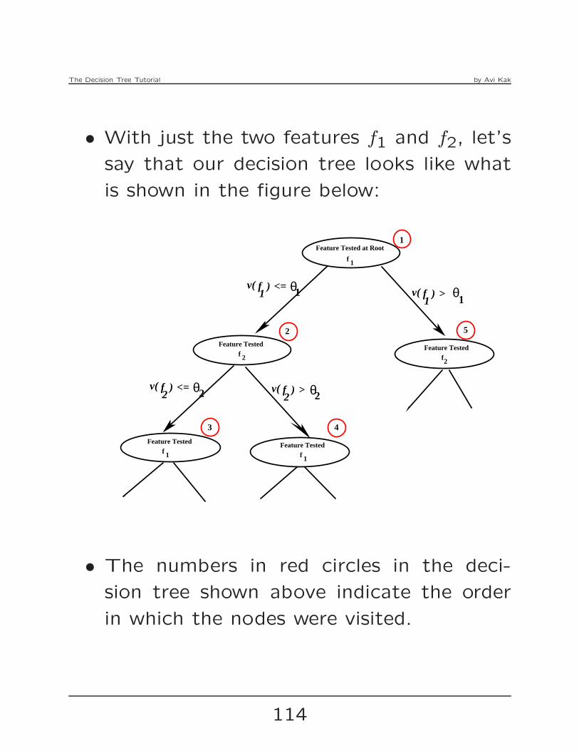
The Decision Tree Tutorial by Avi Kak
• With just the two features f1 and f2, let’s
say that our decision tree looks like what
is shown in the figure below:
f 1
f 1 f 1
Feature Tested Feature Tested
Feature Tested at Root
f 2 f2
Feature Tested Feature Tested
1
2
3 4
5
v( f1
) v( f )1
v( f ) >2
v( f ) <= 2
<= >θ1 θ1
θ2 θ2
• The numbers in red circles in the deci-
sion tree shown above indicate the order
in which the nodes were visited.
114
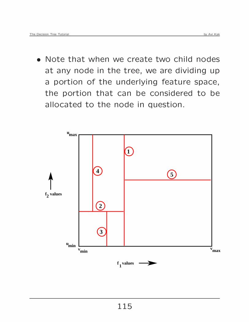
The Decision Tree Tutorial by Avi Kak
• Note that when we create two child nodes
at any node in the tree, we are dividing up
a portion of the underlying feature space,
the portion that can be considered to be
allocated to the node in question.
f values1
f values2
vminvmax
umin
umax
1
2
3
45
115
The Decision Tree Tutorial by Avi Kak
• Each node being in charge of a portion
of the feature space and how it gets par-
titioned when we create two child nodes
there is illustrated by the figure on the
previous page. In this figure, the circled
numbers next to the partitioning lines cor-
respond to the numbers attached to the
nodes in the decision tree on page 65.
• It is good for mental imagery to associate
the entropies we talked about earlier with
the different portions of the feature space.
For example, the entropy H(C | f1<) ob-
viously corresponds to the portion of the
feature space to the left of the vertical di-
viding line that has the number 1 in the fig-
ure. Similarly, the entropy H(C | f1<, f2<)
corresponds to the portion that is to the
left of the vertical dividing line numbered 1
and below the horizontal dividing line num-
bered 2.
116

The Decision Tree Tutorial by Avi Kak
• As we grow the decision tree, our goal must
be to reach the nodes that are pure or until
there is no further reduction in the entropy
in the sense we talked about earlier. A
node is pure if it has zero entropy. Obvi-
ously, the classification made at that node
will be unambiguous.
• After we have finished growing up the tree,
we are ready to convert it into a hash table.
• We first create a sufficiently fine quantiza-
tion of the underlying feature space so that
the partitions created by the decision tree
are to the maximum extent feasible on the
quantization boundaries.
• We are allowed to use different quantiza-
tion intervals along the different features
to ensure the fulfillment of this condition.
117
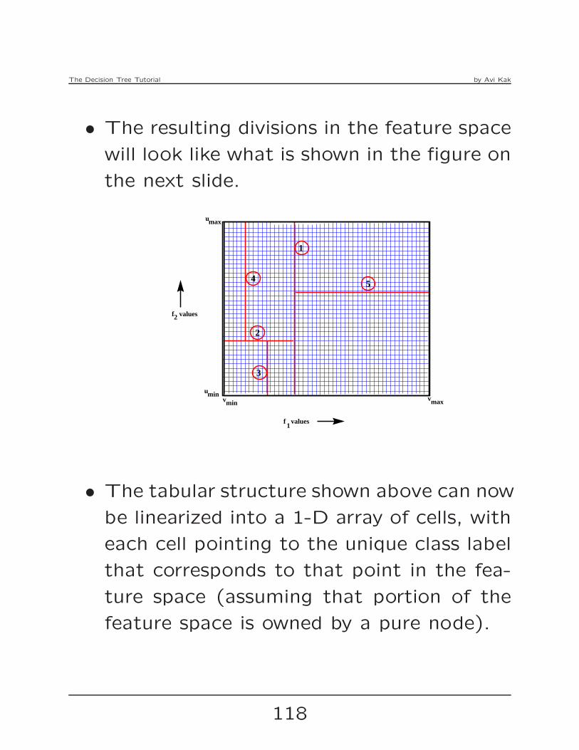
The Decision Tree Tutorial by Avi Kak
• The resulting divisions in the feature space
will look like what is shown in the figure on
the next slide.
f values1
f values2
vminvmax
umin
umax
1
2
3
45
• The tabular structure shown above can now
be linearized into a 1-D array of cells, with
each cell pointing to the unique class label
that corresponds to that point in the fea-
ture space (assuming that portion of the
feature space is owned by a pure node).
118

The Decision Tree Tutorial by Avi Kak
• However, should it be the case that the
portion of the feature space from which
the cell is drawn is impure, the cell in our
linearized structure can point to all of the
applicable class labels and the associated
probabilities.
• The resulting one-dimensional array of cells
lends itself straightforwardly to being stored
as an associative list in the form of a hash
table. For example, if you are using Perl,
you would use the built-in hash data struc-
ture for creating such a hash table. You
can do the same in Python with a dictio-
nary.
119

The Decision Tree Tutorial by Avi Kak
18. Constructing Regression Trees
• So far we have focused exclusively on de-
cision trees. As you should know by this
time, decision tree based modeling requires
that the class labels be distinct. That is,
the training dataset must contain a rela-
tively small number of discrete class labels
for all of your data records if you want to
model the data with one or more decision
trees.
• However, when one is trying to understand
all of the associational relationships that
exist in a large database, one often runs
into situations where, instead of discrete
class labels, you have a continuously val-
ued variable as a dependent variable whose
values are predicated on a set of feature
values.
120

The Decision Tree Tutorial by Avi Kak
• It is for such situations that you will find
useful the new class RegressionTree that is
now a part of the DecisionTree module. If in-
terested in regression, look for the RegressionTree
class in Version 3.4.3 of the Python module
and in Version 3.43 of the Perl module.
• For both the Perl and the Python cases,
the RegressionTree class has been programmed
as a subclass of the main DecisionTree class.
The RegressionTree calls on the DecisionTree
class for several record keeping and some
key low-level data processing steps.
• You can think of regression with a re-
gression tree as a powerful generaliza-
tion of the very commonly used linear
regression algorithms.
121

The Decision Tree Tutorial by Avi Kak
• Although you can certainly carry out poly-
nomial regression with run-of-the-mill lin-
ear regression algorithms for modeling non-
linearities between the predictor variables
and the dependent variable, specifying the
degree of a polynomial is often tricky. Ad-
ditionally, a polynomial can inject continuities be-
tween the predictor and the predicted variables that
may not actually exist in the real data.
• Regression trees, on the other hand, give
you a piecewise linear relationship between
the predictor and the predicted variables
that is freed from the constraints of super-
imposed continuities at the joins between
the different segments.
• See the following tutorial for further in-
formation regarding the standard linear re-
gression approach and the regression that
can be achieved with the RegressionTree class:
https://engineering.purdue.edu/kak/Tutorials/RegressionTree.pdf
122

The Decision Tree Tutorial by Avi Kak
• While linear regression has sufficed for many
applications, there are many others where
it fails to perform adequately. Just to il-
lustrate this point with a simple example,
shown below is some noisy data for which
the linear regression yields the line shown
in red. The blue line is the output of the
tree regression algorithm as implemented
in the RegressionTree class:
123

The Decision Tree Tutorial by Avi Kak
• You will find the RegressionTree class easy to
use in your own scripts. See my Regression
Tree tutorial at:
https://engineering.purdue.edu/kak/Tutorials/RegressionTree.pdf
for how to call the constructor of this class
and how to invoke the functionality incor-
porated in it.
• You will also find example scripts in the
ExamplesRegression subdirectories of the main
installation directory that you can use to
become more familiar with tree regression.
124

The Decision Tree Tutorial by Avi Kak
19. Historical Antecedents of Decision
Tree Classification in Purdue RVL
• During her Ph.D dissertation in the Robot
Vision Lab at Purdue, Lynne Grewe cre-
ated a full-blown implementation of a decision-
tree/hashtable based classifier for recog-
nizing 3D objects in a robotic workcell. It
was a pretty amazing dissertation. She
not only implemented the underlying the-
ory, but also put together a sensor suite for
collecting the data so that she could give
actual demonstrations on a working robot.
• The learning phase in Lynne’s demonstra-
tions consisted of merely showing 3D ob-
jects to the sensor suite. For each object
shown, the human would tell the computer
what its identity and pose was.
125
The Decision Tree Tutorial by Avi Kak
• From the human supplied class labels and
pose information, the computer constructed
a decision tree in the manner described in
the previous sections of this tutorial. Sub-
sequently, the decision tree was converted
into a hash table for fast classification.
• The testing phase consisted of the robot
using the hash table constructed during the
learning phase to recognize the objects and
to estimate their poses. The fact that
the robot successfully manipulated the ob-
jects established for us the viability of using
decision-tree based learning in the context
of robot vision.
• The details of this system are published in
Lynne Grewe and Avinash Kak, "Interactive Learningof a Multi-Attribute Hash Table Classifier forFast Object Recognition," Computer Vision andImage Understanding, pp. 387-416, Vol. 61,No. 3, 1995.
126

The Decision Tree Tutorial by Avi Kak
20. Acknowledgments
In one form or another, decision trees have been aroundfor over fifty years. From a statistical perspective, theyare closely related to classification and regression byrecursive partitioning of multidimensional data. Earlywork that demonstrated the usefulness of such parti-tioning of data for classification and regression can betraced, in the statistics community, to the work done byTerry Therneau in the early 1980’s, and, in the machinelearning community, to the work of Ross Quinlan in themid 1990’s.
I have enjoyed several animated conversations with JoshZapf and Padmini Jaikumar on the topic of decisiontree induction. As a matter of fact, this tutorial wasprompted by conversations with Josh regarding LynneGrewe’s implementation of decision-tree induction forcomputer vision applications. (As I mentioned in Sec-tion 19, Lynne Grewe was a former Ph.D. student ofmine in Purdue Robot Vision Lab.) We are still in somedisagreement regarding the computation of average en-tropies at the nodes of a decision tree. But then lifewould be very dull if people always agreed with one an-other all the time.
127