Decision Tree Learning

Based on “Machine Learning”, T. Mitchell, McGRAW Hill, 1997, ch. 3

Acknowledgement:

The present slides are an adaptation of slides drawn by T. Mitchell

0.

PLAN

• Concept learning: an example

• Decision tree representation

• ID3 learning algorithm

• Statistical measures in decision tree learning:

Entropy, Information gain

• Issues in DT Learning:

1. Inductive bias in ID3

2. Avoiding overfitting of data

3. Incorporating continuous-valued attributes

4. Alternative measures for selecting attributes

5. Handling training examples with missing attributes values

6. Handling attributes with different costs

1.

1. Concept learning: an exampleGiven the data:

Day Outlook Temperature Humidity Wind PlayTennis

D1 Sunny Hot High Weak No

D2 Sunny Hot High Strong No

D3 Overcast Hot High Weak Yes

D4 Rain Mild High Weak Yes

D5 Rain Cool Normal Weak Yes

D6 Rain Cool Normal Strong No

D7 Overcast Cool Normal Strong Yes

D8 Sunny Mild High Weak No

D9 Sunny Cool Normal Weak Yes

D10 Rain Mild Normal Weak Yes

D11 Sunny Mild Normal Strong Yes

D12 Overcast Mild High Strong Yes

D13 Overcast Hot Normal Weak Yes

D14 Rain Mild High Strong No

predict the value of PlayTennis for

〈Outlook = sunny, Temp = cool, Humidity = high, Wind = strong〉

2.

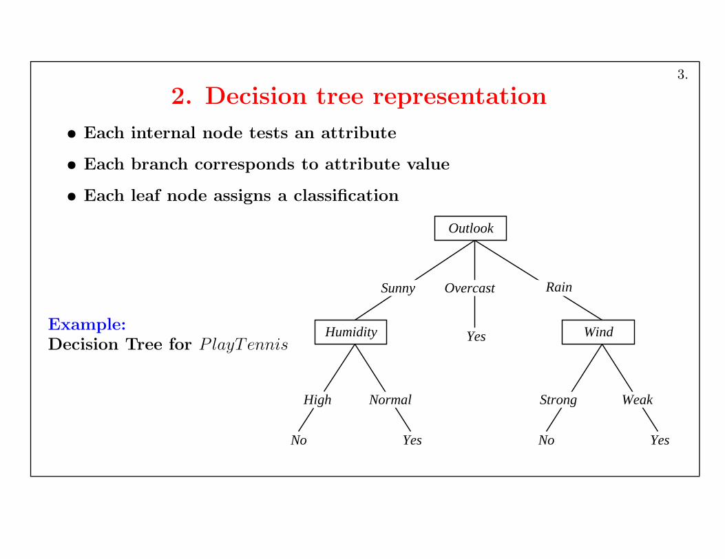
2. Decision tree representation

• Each internal node tests an attribute

• Each branch corresponds to attribute value

• Each leaf node assigns a classification

Example:

Decision Tree for P layTennis

Outlook

Overcast

Humidity

NormalHigh

No Yes

Wind

Strong Weak

No Yes

Yes

RainSunny

3.

Another example:

A Tree to Predict C-Section Risk

Learned from medical records of 1000 women

Negative examples are C-sections

[833+,167-] .83+ .17-

Fetal_Presentation = 1: [822+,116-] .88+ .12-

| Previous_Csection = 0: [767+,81-] .90+ .10-

| | Primiparous = 0: [399+,13-] .97+ .03-

| | Primiparous = 1: [368+,68-] .84+ .16-

| | | Fetal_Distress = 0: [334+,47-] .88+ .12-

| | | | Birth_Weight < 3349: [201+,10.6-] .95+ .05-

| | | | Birth_Weight >= 3349: [133+,36.4-] .78+ .22-

| | | Fetal_Distress = 1: [34+,21-] .62+ .38-

| Previous_Csection = 1: [55+,35-] .61+ .39-

Fetal_Presentation = 2: [3+,29-] .11+ .89-

Fetal_Presentation = 3: [8+,22-] .27+ .73-

4.

When to Consider Decision Trees

• Instances describable by attribute–value pairs

• Target function is discrete valued

• Disjunctive hypothesis may be required

• Possibly noisy training data

Examples:

• Equipment or medical diagnosis

• Credit risk analysis

• Modeling calendar scheduling preferences

5.

3. ID3 Algorithm:

Top-Down Induction of Decision Trees

START

create the root node;

assign all examples to root;

Main loop:

1. A← the “best” decision attribute for next node;

2. for each value of A, create a new descendant of node;

3. sort training examples to leaf nodes;

4. if training examples perfectly classified, then STOP;

else iterate over new leaf nodes

6.

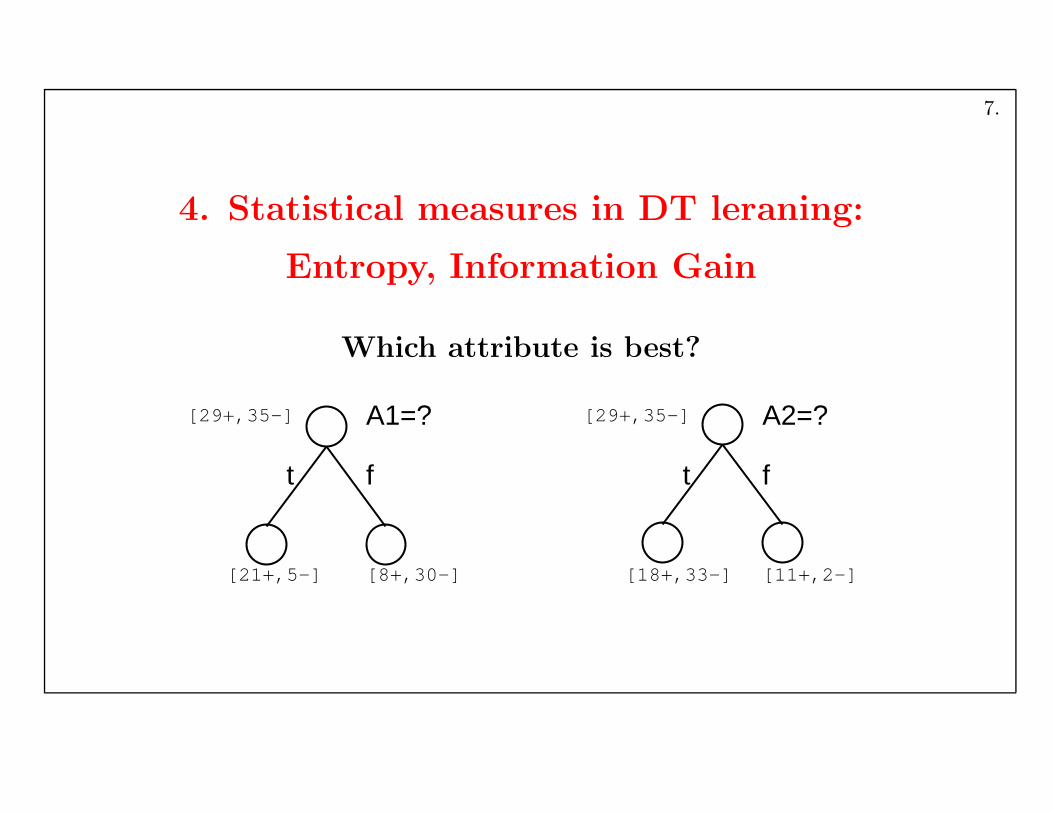
4. Statistical measures in DT leraning:

Entropy, Information Gain

Which attribute is best?

A1=? A2=?

ft ft

[29+,35-] [29+,35-]

[21+,5-] [8+,30-] [18+,33-] [11+,2-]

7.

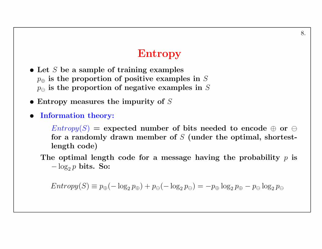
Entropy

• Let S be a sample of training examplesp⊕ is the proportion of positive examples in S

p is the proportion of negative examples in S

• Entropy measures the impurity of S

• Information theory:

Entropy(S) = expected number of bits needed to encode ⊕ or

for a randomly drawn member of S (under the optimal, shortest-length code)

The optimal length code for a message having the probability p is− log

2p bits. So:

Entropy(S) ≡ p⊕(− log2p⊕) + p(− log

2p) = −p⊕ log

2p⊕ − p log

2p

8.

Entropy

Ent

ropy

(S)

1.0

0.5

0.0 0.5 1.0p+

Entropy(S) ≡ −p⊕ log2 p⊕−p log2 p

9.

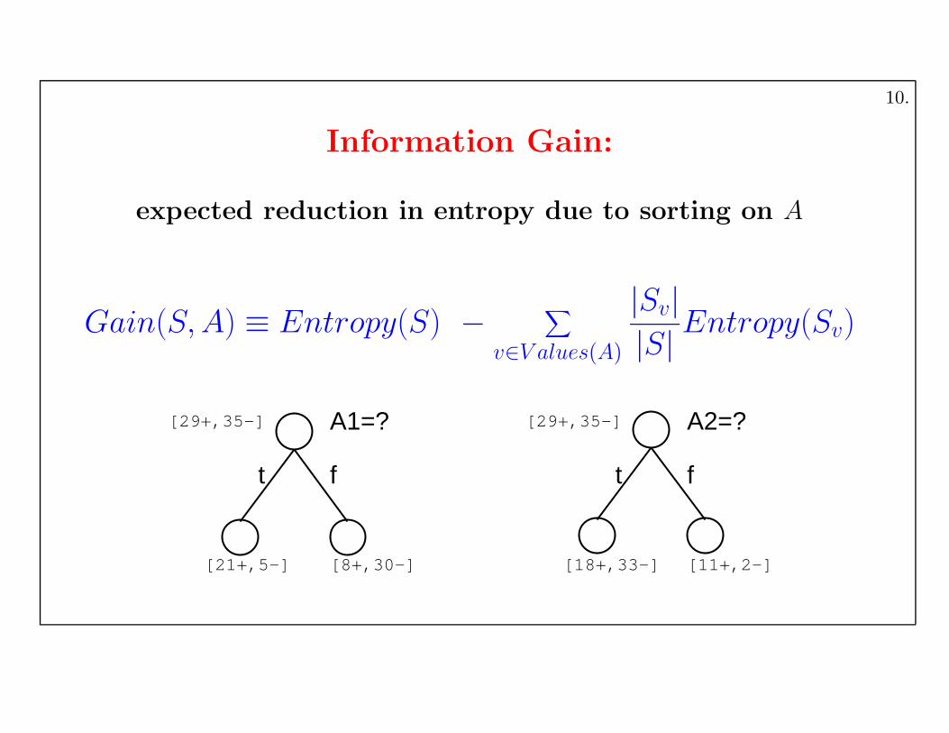
Information Gain:

expected reduction in entropy due to sorting on A

Gain(S, A) ≡ Entropy(S) −∑

v∈V alues(A)

|Sv|

|S|Entropy(Sv)

A1=? A2=?

ft ft

[29+,35-] [29+,35-]

[21+,5-] [8+,30-] [18+,33-] [11+,2-]

10.

Selecting the Next Attribute

Which attribute is the best classifier?

High Normal

Humidity

[3+,4-] [6+,1-]

Wind

Weak Strong

[6+,2-] [3+,3-]

= .940 - (7/14).985 - (7/14).592 = .151

= .940 - (8/14).811 - (6/14)1.0 = .048

Gain (S, Humidity ) Gain (S, )Wind

=0.940E =0.940E

=0.811E=0.592E=0.985E =1.00E

[9+,5-]S:[9+,5-]S:

11.

Partiallylearned tree

Outlook

Sunny Overcast Rain

[9+,5−]

{D1,D2,D8,D9,D11} {D3,D7,D12,D13} {D4,D5,D6,D10,D14}

[2+,3−] [4+,0−] [3+,2−]

Yes

{D1, D2, ..., D14}

? ?

Which attribute should be tested here?

Ssunny = {D1,D2,D8,D9,D11}

Gain (Ssunny , Humidity)

sunnyGain (S , Temperature) = .970 − (2/5) 0.0 − (2/5) 1.0 − (1/5) 0.0 = .570

Gain (S sunny , Wind) = .970 − (2/5) 1.0 − (3/5) .918 = .019

= .970 − (3/5) 0.0 − (2/5) 0.0 = .970

12.

HypothesisSpace Searchby ID3

...

+ + +

A1

+ – + –

A2

A3+

...

+ – + –

A2

A4–

+ – + –

A2

+ – +

... ...

–

13.

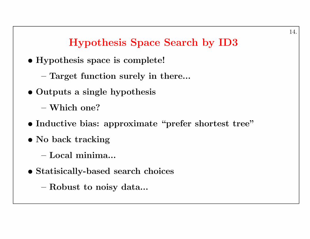
Hypothesis Space Search by ID3

• Hypothesis space is complete!

– Target function surely in there...

• Outputs a single hypothesis

– Which one?

• Inductive bias: approximate “prefer shortest tree”

• No back tracking

– Local minima...

• Statisically-based search choices

– Robust to noisy data...

14.

5. Issues in DT Learning

5.1 Inductive Bias in ID3

Note: H is the power set of instances X

→ Unbiased?

Not really...

• Preference for short trees, and for those with high infor-

mation gain attributes near the root

• Bias is a preference for some hypotheses, rather than a

restriction of hypothesis space H

• Occam’s razor: prefer the shortest hypothesis that fits the

data

15.

Occam’s Razor

Why prefer short hypotheses?

Argument in favor:

• Fewer short hypotheses than long hypsotheses

→ a short hypothesis that fits data unlikely to be coincidence

→ a long hypothesis that fits data might be coincidence

Argument opposed:

• There are many ways to define small sets of hypotheses

(E.g., all trees with a prime number of nodes that use attributes be-

ginning with “Z”.)

• What’s so special about small sets based on size of hypoth-

esis??

16.

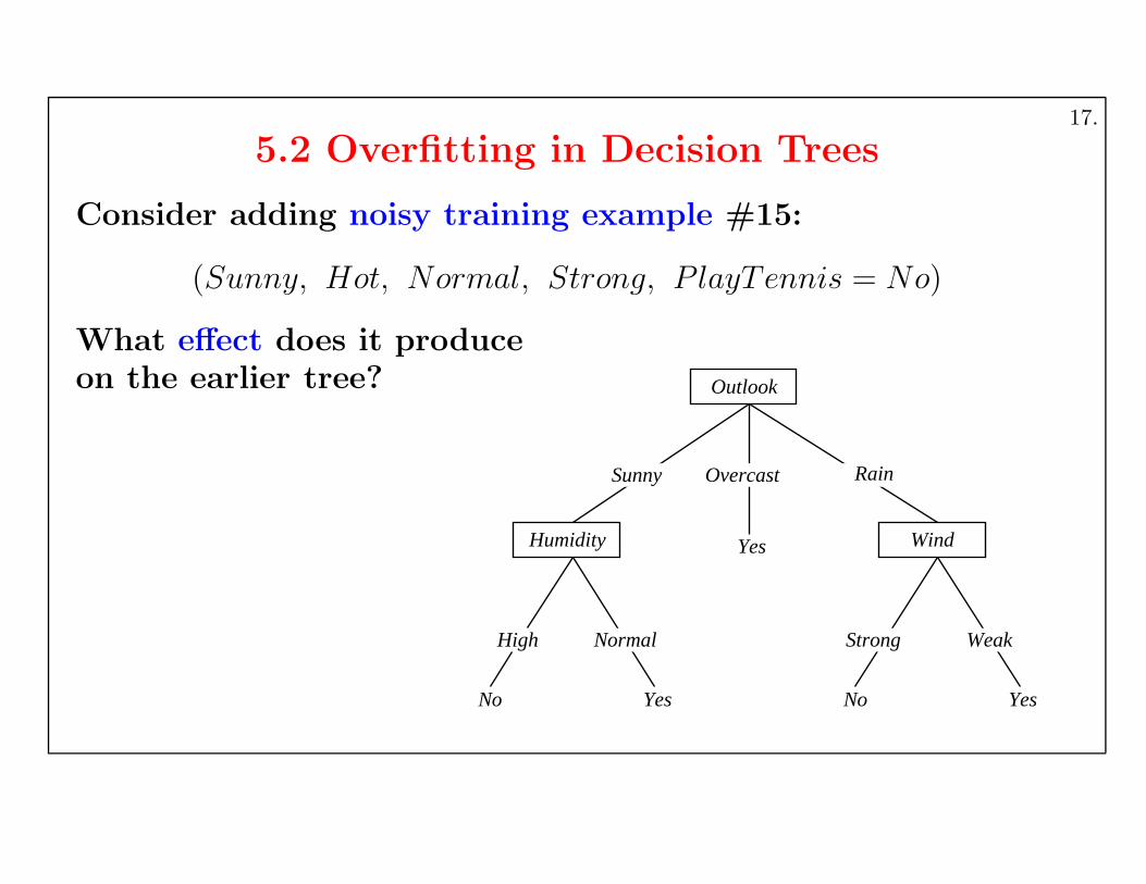
5.2 Overfitting in Decision Trees

Consider adding noisy training example #15:

(Sunny, Hot, Normal, Strong, P layTennis = No)

What effect does it produce

on the earlier tree? Outlook

Overcast

Humidity

NormalHigh

No Yes

Wind

Strong Weak

No Yes

Yes

RainSunny

17.

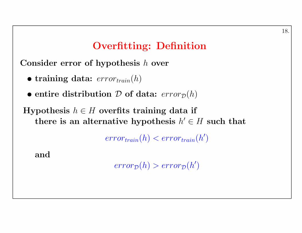
Overfitting: Definition

Consider error of hypothesis h over

• training data: errortrain(h)

• entire distribution D of data: errorD(h)

Hypothesis h ∈ H overfits training data if

there is an alternative hypothesis h′∈ H such that

errortrain(h) < errortrain(h′)

and

errorD(h) > errorD(h′)

18.

Overfitting in Decision Tree Learning

0.5

0.55

0.6

0.65

0.7

0.75

0.8

0.85

0.9

0 10 20 30 40 50 60 70 80 90 100

Acc

urac

y

Size of tree (number of nodes)

On training dataOn test data

19.

Avoiding Overfitting

How can we avoid overfitting?

• stop growing when the data split is not anymore statisti-

cally significant

• grow full tree, then post-prune

How to select “best” tree:

• Measure performance over training data

• Measure performance over a separate validation data set

• MDL: minimize size(tree) + size(misclassifications(tree))

20.

Reduced-Error Pruning

Split data into training set and validation set

Do until further pruning is harmful:

1. Evaluate impact on validation set of pruning each possiblenode (plus those below it)

2. Greedily remove the one that most improves validation setaccuracy

Efect: Produces the smallest version of most accurate subtree

Question: What if data is limited?

21.

Effect of Reduced-Error Pruning

0.5

0.55

0.6

0.65

0.7

0.75

0.8

0.85

0.9

0 10 20 30 40 50 60 70 80 90 100

Acc

urac

y

Size of tree (number of nodes)

On training dataOn test data

On test data (during pruning)

22.

Rule Post-Pruning

1. Convert tree to equivalent set of rules

2. Prune each rule independently of others

3. Sort final rules into desired sequence for use

It is perhaps most frequently used method (e.g., C4.5)

23.

Converting A Tree to Rules

Outlook

Overcast

Humidity

NormalHigh

No Yes

Wind

Strong Weak

No Yes

Yes

RainSunny

IF (Outlook = Sunny) ∧ (Humidity = High)THEN P layTennis = No

IF (Outlook = Sunny) ∧ (Humidity = Normal)THEN P layTennis = Y es

. . .

24.

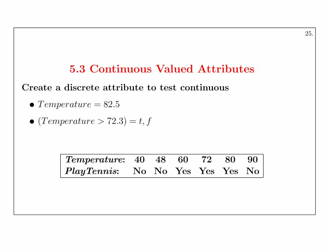
5.3 Continuous Valued Attributes

Create a discrete attribute to test continuous

• Temperature = 82.5

• (Temperature > 72.3) = t, f

Temperature: 40 48 60 72 80 90

PlayTennis: No No Yes Yes Yes No

25.

5.4 Attributes with Many Values

Problem:

• If attribute has many values, Gain will select it

• Imagine using Date = Jun 3 1996 as attribute

One approach: use GainRatio instead

GainRatio(S, A) ≡Gain(S, A)

SplitInformation(S, A)

SplitInformation(S, A) ≡ −c∑

i=1

|Si|

|S|log2

|Si|

|S|

where Si is the subset of S for which A has the value vi

26.

5.5 Attributes with Costs

Consider

• medical diagnosis, BloodTest has cost $150

• robotics, Width from 1ft has cost 23 sec.

Question: How to learn a consistent tree with low expected

cost?One approach: replace gain by

•Gain2(S,A)

Cost(A) (Tan and Schlimmer, 1990)

•2Gain(S,A)

−1(Cost(A)+1)w (Nunez, 1988)

where w ∈ [0, 1] determines importance of cost

27.

5.6 Unknown Attribute Values

Question: What if an example is missing the value of an at-

tribute A?

Use the training example anyway, sort through tree

• If node n tests A, assign the most common value of A among

the other examples sorted to node n

• assign the most common value of A among the other ex-

amples with same target value

• assign probability pi to each possible value vi of A

– assign the fraction pi of the example to each descendant

in the tree

Classify new examples in same fashion.

28.