decision diagrams for discrete...
TRANSCRIPT

Decision Diagrams
for Discrete Optimization
John HookerCarnegie Mellon University
ICAPS Tutorial
London, June 2016

Companion Tutorial:
Decision Diagrams
for Sequencing and Scheduling
Willem-Jan van HoeveCarnegie Mellon University
Immediately follows this tutorial

Decision Diagrams
• Used in computer science and AI for decades
– Logic circuit design
– Product configuration
• A new perspective on optimization
– Constraint programming
– Discrete optimization
3
Decision Diagrams
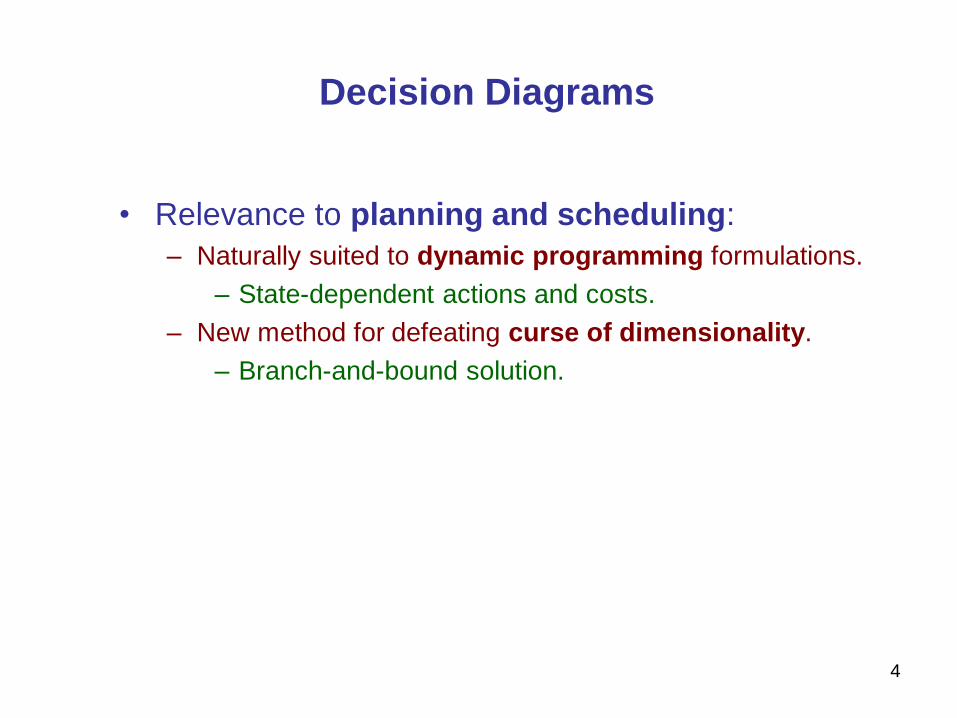
• Relevance to planning and scheduling:
– Naturally suited to dynamic programming formulations.
– State-dependent actions and costs.
– New method for defeating curse of dimensionality.
– Branch-and-bound solution.
4

Decision Diagrams
• DDs have been used in planning literature…
– To encode (or approximate) state-dependent cost or
cost-to-go.
– See yesterday’s tutorial “Planning with State-Dependent
Action Costs”
– By Robert Mattmüller and Florian Geißer.
• This tutorial presents DDs as a general
optimization method.
5

Decision Diagrams
• General advantages:
– No need for inequality formulations.
– No need for linear or convex relaxations.
– New approach to solving dynamic programming models.
– Very effective parallel computation.
– Ideal for postoptimality anaylsis
• Disadvantage:
– Developed only for discrete, deterministic optimization.
– …so far.
6

Outline
• Decision diagram basics
• Optimization with exact decision diagrams
• A general-purpose solver that scales up
– Relaxed decision diagrams
– Restricted decision diagrams
– Dynamic programming model
– A new branching algorithm
– Computational performance
• Modeling the objective function
– Inventory management example
• Nonserial decision diagrams
• References 7
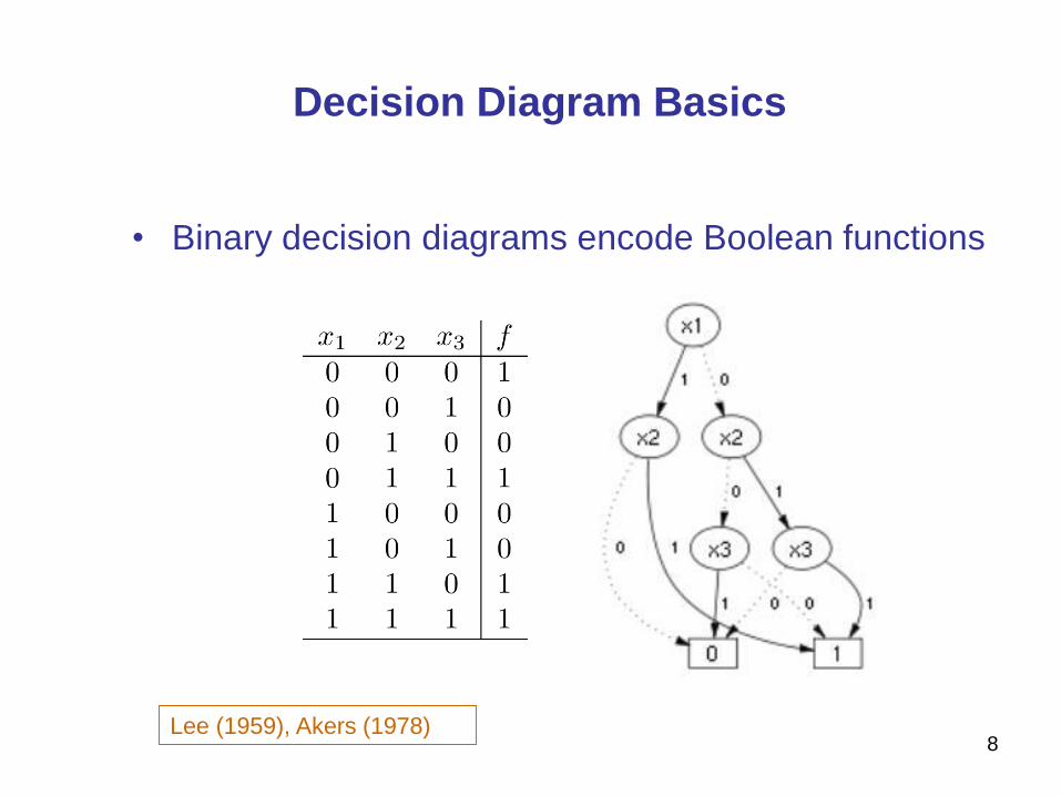
Decision Diagram Basics
• Binary decision diagrams encode Boolean functions
8Lee (1959), Akers (1978)

Decision Diagram Basics
• Binary decision diagrams encode Boolean functions
– Historically used for circuit design & verification
9Bryant (1986), etc.
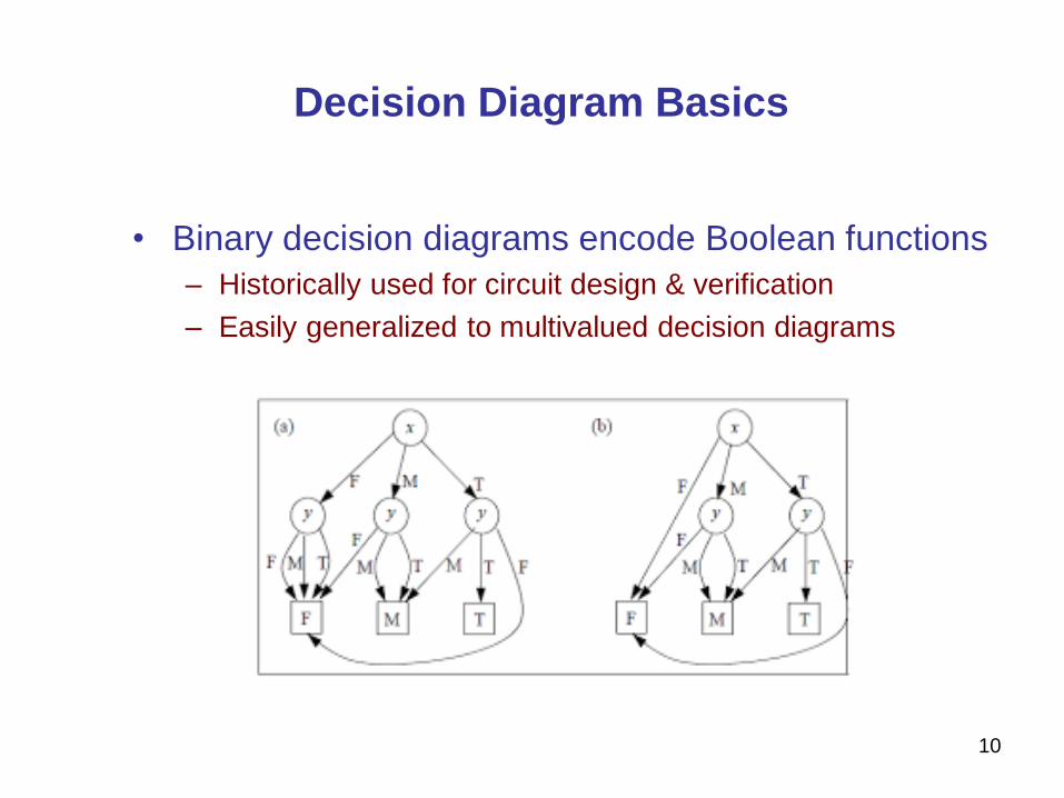
Decision Diagram Basics
• Binary decision diagrams encode Boolean functions
– Historically used for circuit design & verification
– Easily generalized to multivalued decision diagrams
10

Reduced Decision Diagrams
• There is a unique reduced DD representing any given
Boolean function.
– Once the variable ordering is specified.
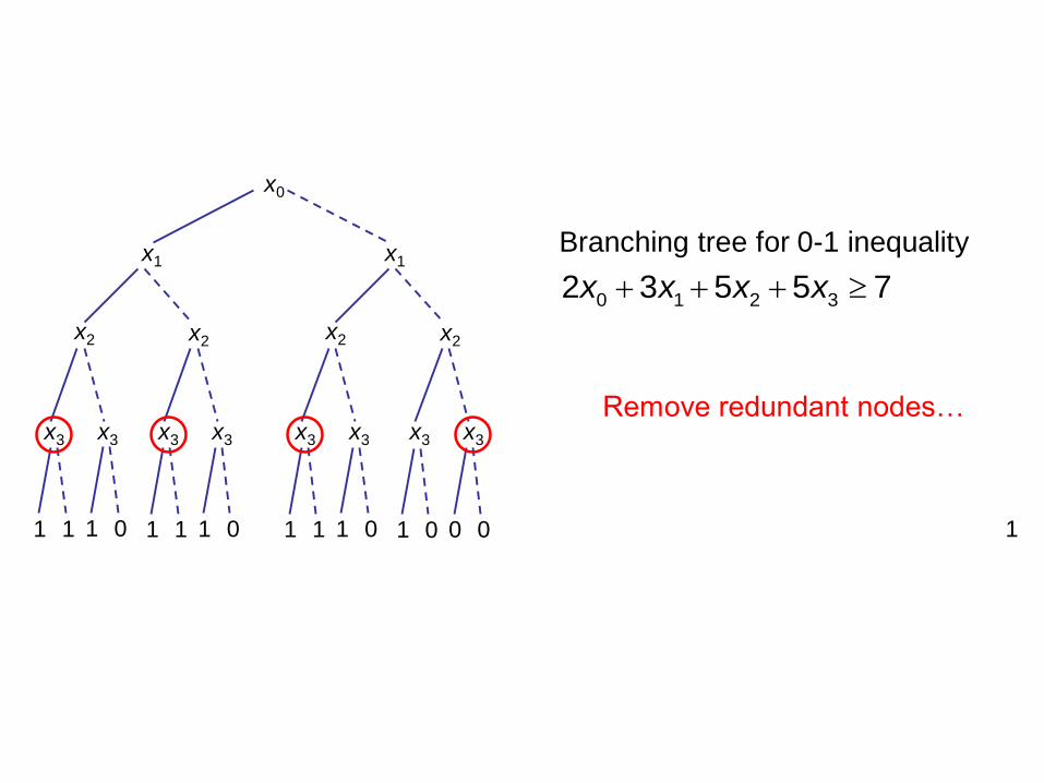
• The reduced DD can be viewed as a branching tree with
redundancy removed.
– Superimpose isomorphic subtrees.
– Remove redundant nodes.
Bryant (1986)

x0
x1
x2 x2
x3 x3 x3 x3
1 1
x1
x2 x2
x3 x3 x3 x3
1 0 1 1 1 0 1 1 1 0 1 0 0 0 1
Branching tree for 0-1 inequality
1 indicates feasible solution,
0 infeasible
0 1 2 32 3 5 5 7x x x x
0 1x 0 0x
x0
x1
x2 x2
x3 x3 x3 x3
1 1
x1
x2 x2
x3 x3 x3 x3
1 0 1 1 1 0 1 1 1 0 1 0 0 0 1
Remove redundant nodes…
Branching tree for 0-1 inequality
0 1 2 32 3 5 5 7x x x x

x0
x1
x2 x2
x3 x3 x3 x3
1 1
x1
x2 x2
x3 x3 x3 x3
1 0 1 1 1 0 1 1 1 0 1 0 0 0
x0
x1
x2 x2
x3
1
x1
x2 x2
0
x3
1 0
x3
1 0
x3
011 1 1 0

x0
x1
x2 x2
x3
1
x1
x2 x2
0
x3
1 0
x3
1 0
x3
01
Superimpose identical
subtrees…
1 1 1 0

x0
x2
x1
x2
x3
1 0
x3
1 0
x0
x1
x2 x2
x3
1
x1
x2 x2
0
x3
1 0
x3
1 0
x3
011 1 1 01 0

x0
x2
x1
x2
x3
1 0
x3
1 01 0
Superimpose identical
subtrees…

x0
x2
x1
x2
x3
1 0
x3
1 01 0
x0
x2
x1
x2
x3
1 0 01

x0
x2
x1
x2
x3
1 0 01
Superimpose identical
leaf nodes…

x0
x2
x1
x2
x3
1 0
x0
x2
x1
x2
x3
1 0 01

as generated by software
x0
x2
x1
x2
x3
1 0

Reduced Decision Diagrams
• Reduced DD for a knapsack constraint can be
surprisingly small…
The 0-1 inequality
has 117,520 maximal feasible solutions (or minimal covers)
But its reduced BDD has only 152 nodes…
0 1 2 3 4 5 6 7 8 9
10 11 12 13 14 15 16 17 18
300 300 285 285 265 265 230 230 190 200
400 200 400 200 400 200 400 200 400 2700
x x x x x x x x x x
x x x x x x x x x


Optimization with Exact Decision
Diagrams
24
• Decision diagrams can
represent feasible set
– Remove paths to 0.
– Paths to 1 are feasible
solutions.
– Associate costs with
arcs.
– Find longest/shortest
path
Hadžić and JH (2006, 2007)

1
2 3
5 4
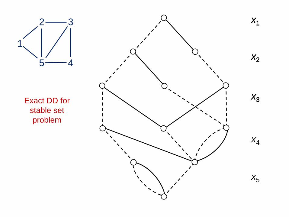
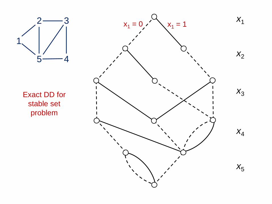
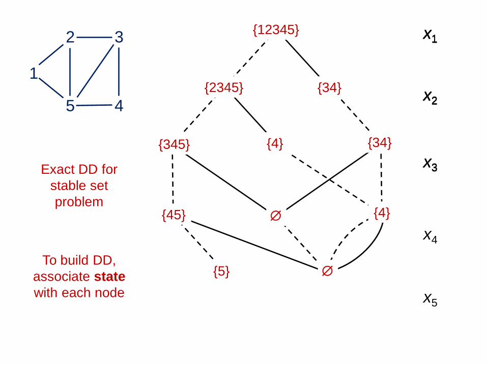
Stable Set Problem
x1
x2
x3
x4
x5
Exact DD for
stable set
problem
1
2 3
5 4
x1
x2
x3
Exact DD for
stable set
problem
1
2 3
5 4
x1 = 1x1 = 0
x4
x5
x1
x2
x3

1
2 3
5 4
x1 = 1x1 = 0
Paths from top
to bottom
correspond to
the 9 feasible
solutions x4
x5
x1
x2
x3

1
2 3
5 4
For objective
function,
associate
weights with
arcs x4
x5
x1
x2
x3
20
40
5050
10
10
30
0
0 0
00
0
00
0
00
20
40 50
30 10

For objective
function,
associate
weights with
arcs x4
x5
x1
x2
x3
Optimal solution
is longest path
1
2 3
5 4
For objective
function,
associate
weights with
arcs
20
40
5050
10
10
30
0
0 0
00
0
00
0
00
20
40 50
30 10

For objective
function,
associate
weights with
arcs x4
x5
x1
x2
x3
20
40
5050
10
10
30
0
0 0
00
0
00
0
00
Optimal solution
is longest path
1
2 3
5 4
20
40 50
30 10
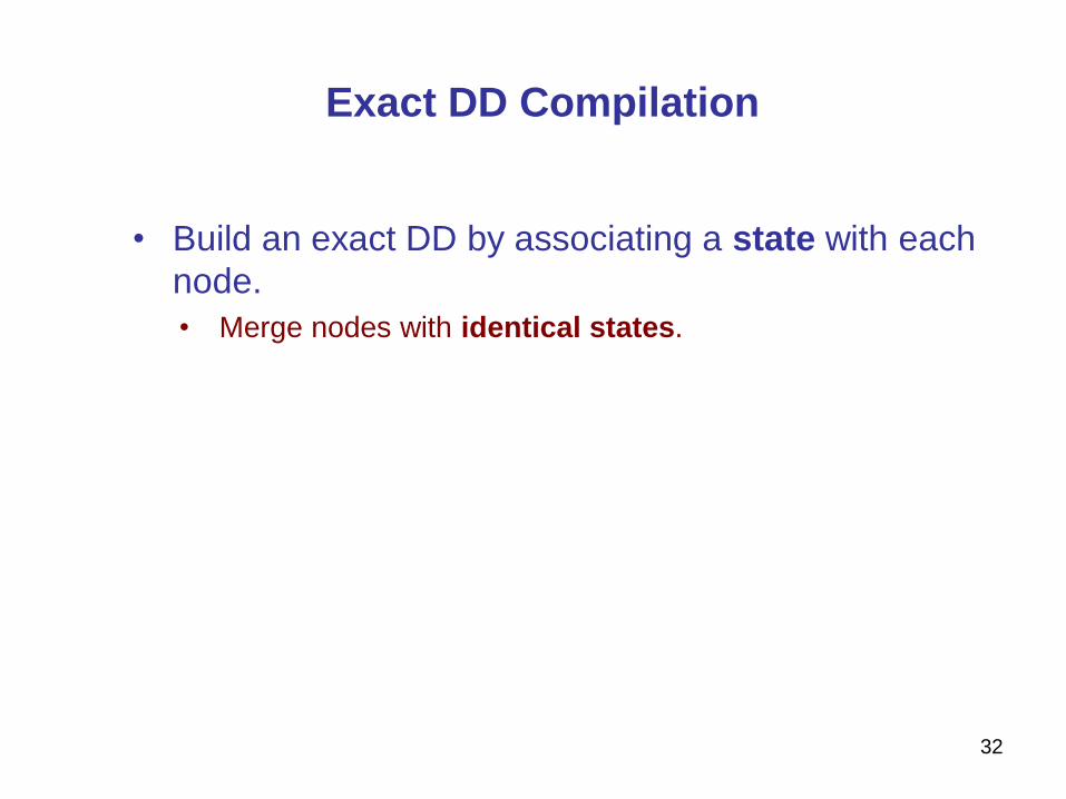
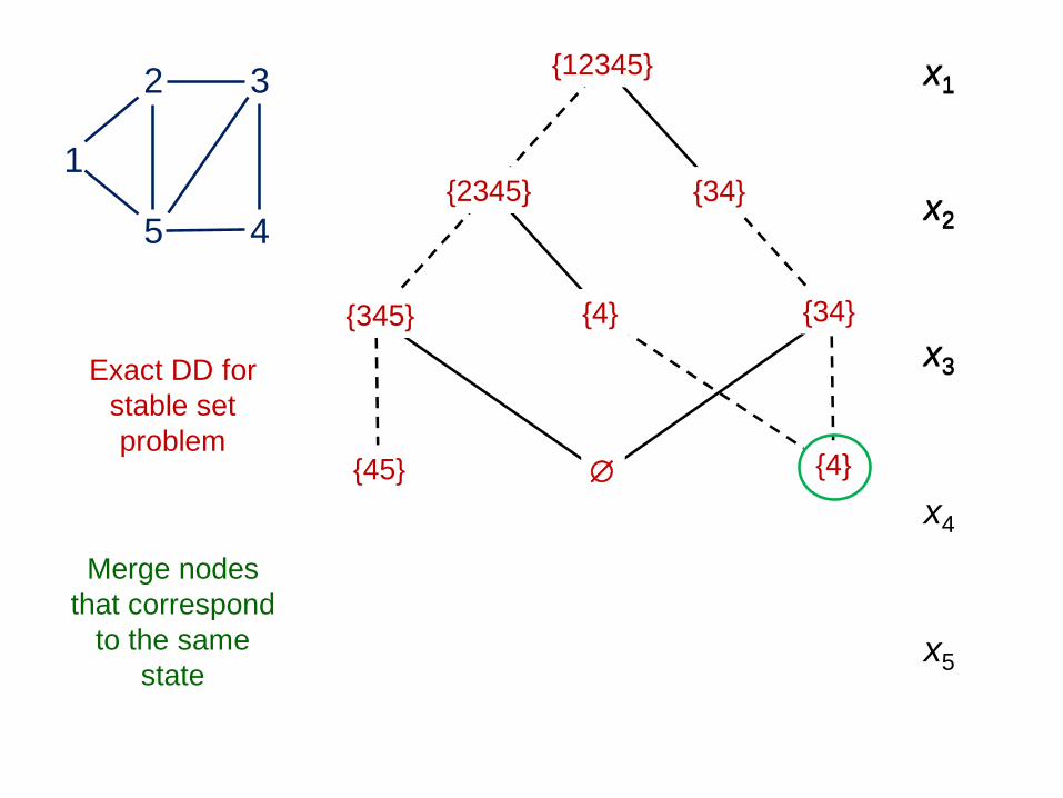
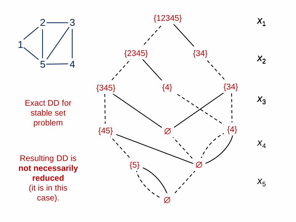
Exact DD Compilation
• Build an exact DD by associating a state with each
node.
• Merge nodes with identical states.
32

x1
x2
x3
x4
x5
Exact DD for
stable set
problem
1
2 3
5 4
x1
x2
x3
{12345}
{2345} {34}
{345} {4} {34}
{45} {4}
{5}
To build DD,
associate state
with each node

x1
x2
x3
x4
x5
Exact DD for
stable set
problem
1
2 3
5 4
x1
x2
x3
{12345}
To build DD,
associate state
with each node

x1
x2
x3
x4
x5
Exact DD for
stable set
problem
1
2 3
5 4
x1
x2
x3
{12345}
{2345} {34}
To build DD,
associate state
with each node

x1
x2
x3
x4
x5
Exact DD for
stable set
problem
1
2 3
5 4
x1
x2
x3
{12345}
{2345} {34}
{345} {4} {34}
To build DD,
associate state
with each node

x1
x2
x3
x4
x5
Exact DD for
stable set
problem
1
2 3
5 4
x1
x2
x3
{12345}
{2345} {34}
{345} {4} {34}
{45} {4}
Merge nodes
that correspond
to the same
state
{4}
x1
x2
x3
x4
x5
Exact DD for
stable set
problem
1
2 3
5 4
x1
x2
x3
{12345}
{2345} {34}
{345} {4} {34}
{45} {4}
Merge nodes
that correspond
to the same
state
x1
x2
x3
x4
x5
Exact DD for
stable set
problem
1
2 3
5 4
x1
x2
x3
{12345}
{2345} {34}
{345} {4} {34}
{45} {4}
{5}
To build DD,
associate state
with each node
x1
x2
x3
x4
x5
Exact DD for
stable set
problem
1
2 3
5 4
x1
x2
x3
{12345}
{2345} {34}
{345} {4} {34}
{45} {4}
{5}
Resulting DD is
not necessarily
reduced
(it is in this
case).

A General-Purpose Solver
• The decision diagram tends to grow exponentially.
• To build a practical solver:
– Use limited-width relaxed decision diagrams to bound the
objective value.
– Use limited-width restricted decision diagrams for primal
heuristic
– Use a recursive dynamic programming model.
– Use novel branching scheme within relaxed decision
diagrams.
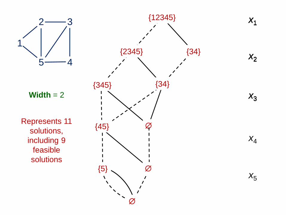
Relaxed Decision Diagrams
• A relaxed DD represents a superset of feasible set.
– Shortest (longest) path length is a bound on optimal value.
– Size of DD is controlled.
– Analogous to LP relaxation in IP, but discrete.
– Does not require linearity, convexity, or inequality constraints.
Andersen, Hadžić, JH, Tiedemann (2007)

x1
x2
x3
x4
x5
1
2 3
5 4
x1
x2
x3
{12345}
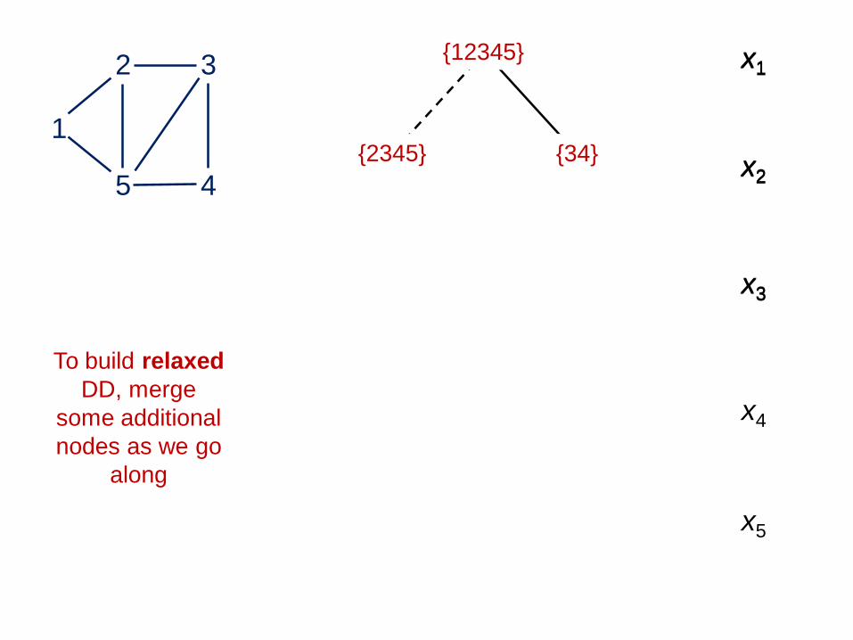
To build relaxed
DD, merge
some additional
nodes as we go
along
x1
x2
x3
x4
x5
1
2 3
5 4
x1
x2
x3
{12345}
{2345} {34}
To build relaxed
DD, merge
some additional
nodes as we go
along

x1
x2
x3
x4
x5
1
2 3
5 4
x1
x2
x3
{12345}
{2345} {34}
{345} {4} {34}
To build relaxed
DD, merge
some additional
nodes as we go
along.
Take the union
of merged
states

x1
x2
x3
x4
x5
1
2 3
5 4
x1
x2
x3
{12345}
{2345} {34}
{345} {34}
To build relaxed
DD, merge
some additional
nodes as we go
along.
Take the union
of merged
states.

x1
x2
x3
x4
x5
1
2 3
5 4
x1
x2
x3
{12345}
{2345} {34}
{345} {34}
{45} {4}To build relaxed
DD, merge
some additional
nodes as we go
along.
Take the union
of merged
states.

x1
x2
x3
x4
x5
1
2 3
5 4
x1
x2
x3
{12345}
{2345} {34}
{345} {34}
{45}
{5}
To build relaxed
DD, merge
some additional
nodes as we go
along.
Take the union
of merged
states.
x1
x2
x3
x4
x5
1
2 3
5 4
x1
x2
x3
{12345}
{2345} {34}
{345} {34}
{45}
{5}
Represents 11
solutions,
including 9
feasible
solutions
Width = 2
x1
x2
x3
x4
x5
x1
x2
x3
{12345}
{2345} {34}
{345} {34}
{45}
{5}
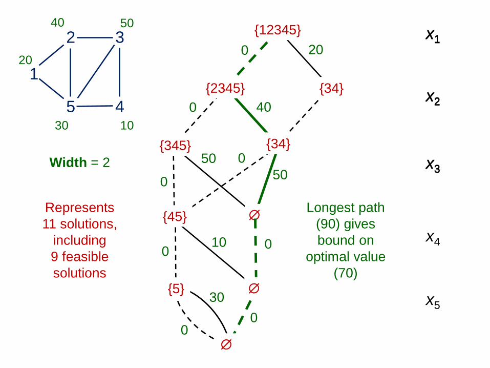
Represents
11 solutions,
including
9 feasible
solutions
Width = 2
Longest path
(90) gives
bound on
optimal value
(70)
20
40
0
0
050
10
0
0
0
1
2 3
5 4
20
40 50
30 10
50
30
0
0

Relaxed Decision Diagrams
• Alternate relaxation method: node refinement.
– Start with DD of width 1 representing Cartesian product of
variable domains.
– Split nodes so as to remove some infeasible paths.
– Will be illustrated in next tutorial.
51
Andersen, Hadžić, JH, Tiedemann (2007)
Relaxed Decision Diagrams
• Original application: enhanced propagation in
constraint programming
– In multiple alldiff problem (graph coloring), reduced
1 million node search trees to 1 node.
52
Andersen, Hadžić, JH, Tiedemann (2007)
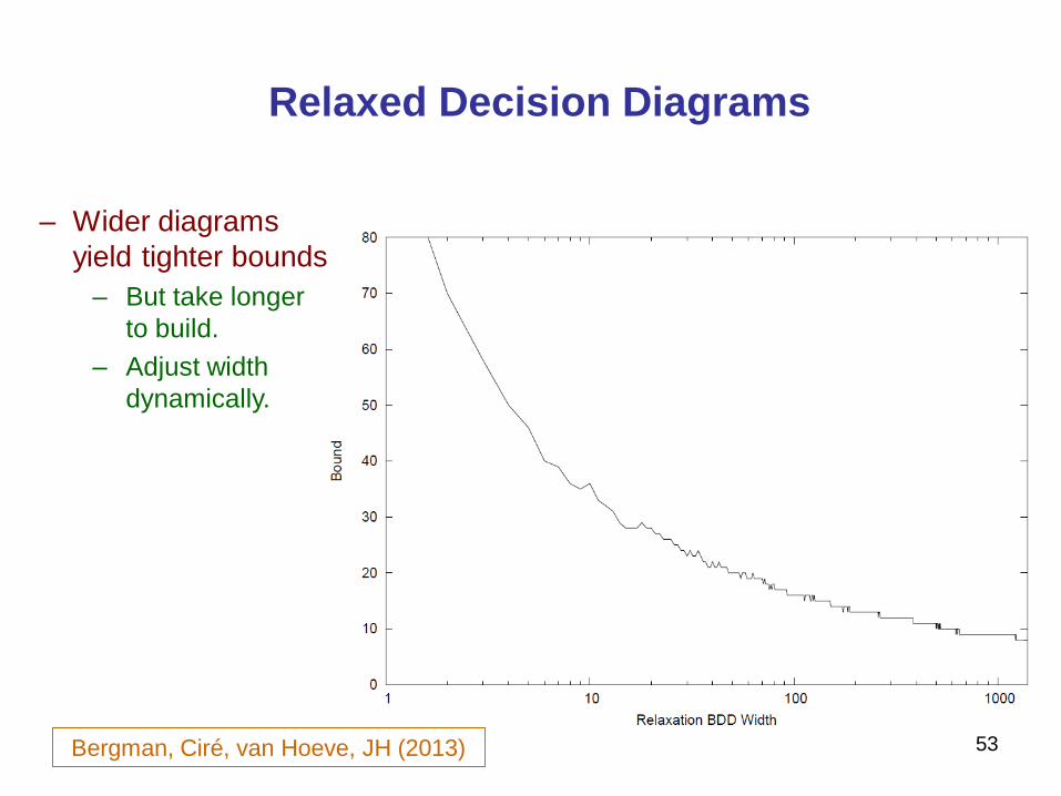
Relaxed Decision Diagrams
– Wider diagrams
yield tighter bounds
– But take longer
to build.
– Adjust width
dynamically.
53Bergman, Ciré, van Hoeve, JH (2013)

Relaxed Decision Diagrams
– DDs vs. CPLEX
bound at root node
for max stable set
problem
– Using CPLEX
default cut
generation
– DD max width
of 1000.
– DDs require
about 5% the
time of CPLEX
54
Bergman, Ciré,
van Hoeve, JH (2013)
CPLEX bound
is better
DD bound
is better

Restricted Decision Diagrams
● A restricted DD represents a subset of the feasible set.
● Restricted DDs provide a basis for a primal heuristic.
– Shortest (longest) paths in the restricted DD provide good
feasible solutions.
– Generate a limited-width restricted DD by deleting nodes that
appear unpromising.
Bergman, Ciré, van Hoeve, Yunes (2014)
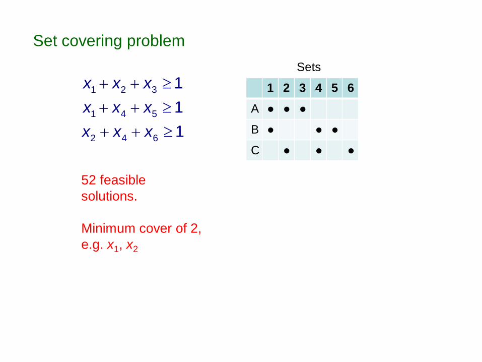
Set covering problem
1 2 3
1 4 5
2 4 6
1
1
1
x x x
x x x
x x x
52 feasible
solutions.
Minimum cover of 2,
e.g. x1, x2
Sets
1 2 3 4 5 6
A ● ● ●
B ● ● ●
C ● ● ●

Restricted DD of width 4
41 paths (< 52 feasible solutions)
Several shortest paths have
length 2.
All are minimum covers.

Restricted DD of width 4
41 paths (< 52 feasible solutions)
Several shortest paths have
length 2.
All are minimum covers.
In this case, restricted DD
delivers optimal solutions.

Optimality gap for set covering, n variables
Restricted DDs vs
Primal heuristic at root node of CPLEX
IP
DD

Computation time
Restricted DDs vs
Primal heuristic at root node of CPLEX (cuts turned off)
IP
DD
IP
DD

Dynamic Programming Model
● Formulate problem with dynamic programming model.
– Rather than constraint set.
– Problem must have recursive structure
– But there is great flexibility to represent constraints and
objective function.
– Any function of current state is permissible.
– We don’t care if state space is exponential, because we don’t
solve the problem by dynamic programming.
● State variables are the same as in relaxed DD.
– Must also specify state merger rule.
Dynamic Programming Model
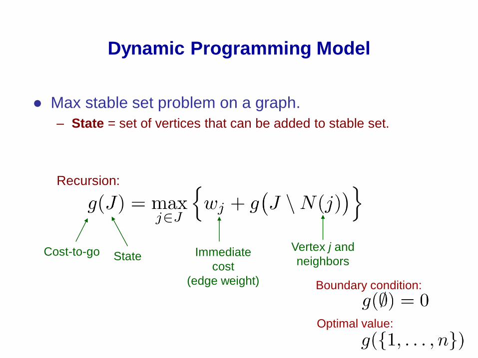
● Max stable set problem on a graph.
– State = set of vertices that can be added to stable set.
Recursion:
Cost-to-go State Immediate
cost
(edge weight)
Vertex j and
neighbors
Boundary condition:
Optimal value:

Dynamic Programming Model
● Max stable set problem on a graph.
– State = set of vertices that can be added to stable set.
– State merger = union
Recursion:
Merger of states in M =
Cost-to-go State Immediate
cost
(edge weight)
Vertex j and
neighbors
Boundary condition:
Optimal value:

Dynamic Programming Model
● Single-machine scheduling with due dates
Minimize total tardiness.
– State = (set of jobs not yet processed,
latest finish time of jobs processed so far)
Cost-to-go
Jobs
remaining
Tardiness of
job j
Boundary condition:
Optimal value:
Last
finish
time

Dynamic Programming Model
● Single-machine scheduling with due dates
Minimize total tardiness.
– State = (set of jobs not yet processed,
latest finish time of jobs processed so far)
– State merger = union, min
Merger of states in M =
Cost-to-go
Jobs
remaining
Tardiness of
job j
Boundary condition:
Optimal value:
Last
finish
time
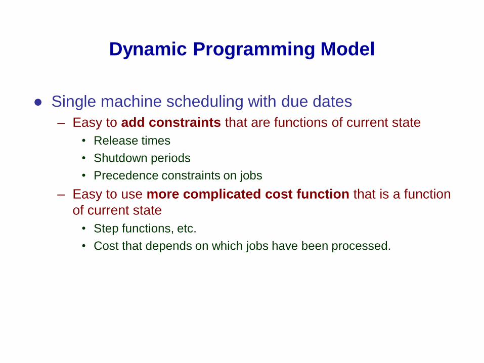
Dynamic Programming Model
● Single machine scheduling with due dates
– Easy to add constraints that are functions of current state
• Release times
• Shutdown periods
• Precedence constraints on jobs
– Easy to use more complicated cost function that is a function
of current state
• Step functions, etc.
• Cost that depends on which jobs have been processed.

Dynamic Programming Model
● Scheduling with sequence-dependent setup times
– State = (Ji, last job processed, fi )
– State merger requires modification of states
Last job
processedProcessing + setup timeTardiness of job j

Dynamic Programming Model
● Scheduling with sequence-dependent setup times
– To allow for state merger:
– State = ( , set of pairs , representing jobs
that could have been the last processed)
Merger of states in M =

Dynamic Programming Model
● Max cut problem on a graph.
– Partition nodes into 2 sets so as to maximize total weight
of connecting edges.
– State = marginal benefit of placing each remaining vertex on left
side of cut.
– State merger =
• Componentwise min if all components 0 or all 0; 0 otherwise
• Adjust incoming arc weights
● Max 2-SAT.
– Similar to max cut.

Branching Algorithm
• Solve optimization problem using a novel
branch-and-bound algorithm.
– Branch on nodes in last exact layer of relaxed decision
diagram.
– …rather than branch on variables.
– Create a new relaxed DD rooted at each branching node.
– Prune search tree using bounds from relaxed DD.
71
Bergman, Ciré, van Hoeve, JH (2016)

● Solve optimization problem using a novel
branch-and-bound algorithm.
– Branch on nodes in last exact layer of relaxed decision
diagram.
– …rather than branch on variables.
– Create a new relaxed DD rooted at each branching node.
– Prune search tree using bounds from relaxed DD.
– Advantage: a manageable number states may be
reachable in first few layers.
– …even if the state space is exponential.
– Alternative way of dealing with curse of dimensionality.
72
Branching Algorithm
Bergman, Ciré, van Hoeve, JH (2016)

1
2
3
4
5
6
Diagram is exact
down to here
Branching in a relaxed
decision diagram
73
Branching Algorithm

Branch on nodes
in this layer
Branching in a relaxed
decision diagram
74
1
2
3
4
5
6
Branching Algorithm
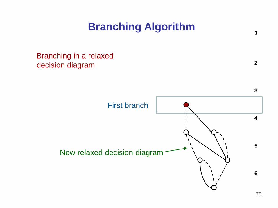
First branch
New relaxed decision diagram
Branching in a relaxed
decision diagram
75
1
2
3
4
5
6
Branching Algorithm

First branch
New relaxed decision diagram
Branching in a relaxed
decision diagram
76
1
2
3
4
5
6
Branching Algorithm
Prune this branch if cost bound from
relaxed DD is no better than cost
of best feasible solution found so far
(branch and bound).
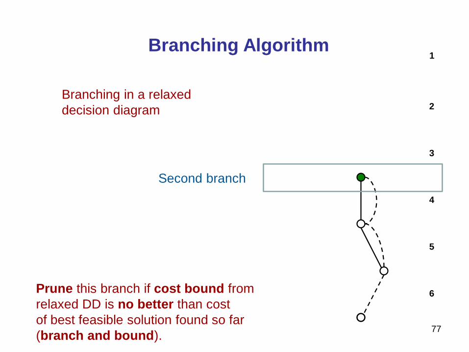
Second branch
Branching in a relaxed
decision diagram
77
1
2
3
4
5
6
Branching Algorithm
Prune this branch if cost bound from
relaxed DD is no better than cost
of best feasible solution found so far
(branch and bound).

Third branch
Continue recursively
Branching in a relaxed
decision diagram
78
1
2
3
4
5
6
Branching Algorithm
Prune this branch if cost bound from
relaxed DD is no better than cost
of best feasible solution found so far
(branch and bound).
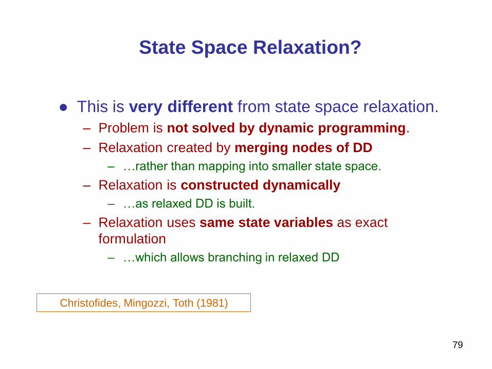
● This is very different from state space relaxation.
– Problem is not solved by dynamic programming.
– Relaxation created by merging nodes of DD
– …rather than mapping into smaller state space.
– Relaxation is constructed dynamically
– …as relaxed DD is built.
– Relaxation uses same state variables as exact
formulation
– …which allows branching in relaxed DD
79
State Space Relaxation?
Christofides, Mingozzi, Toth (1981)
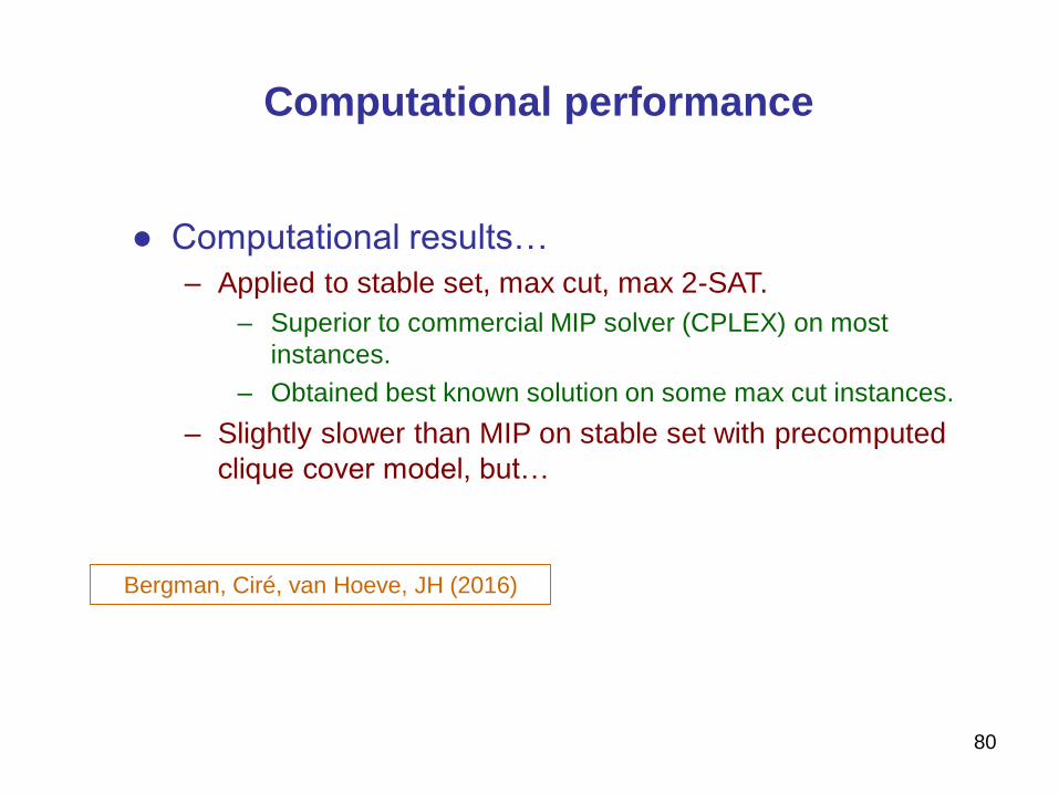
Computational performance
● Computational results…
– Applied to stable set, max cut, max 2-SAT.
– Superior to commercial MIP solver (CPLEX) on most
instances.
– Obtained best known solution on some max cut instances.
– Slightly slower than MIP on stable set with precomputed
clique cover model, but…
80
Bergman, Ciré, van Hoeve, JH (2016)

Max cut
on a graph
Avg. solution time
vs
graph density
30 vertices
0
10
20
30
40
50
60
70
80
0 0.2 0.4 0.6 0.8 1
Avera
ge s
olu
tion t
ime (
sec)
Density of graph
CPLEX
MDDs
Computational performance

Max 2-SAT
Performance
profile
30 variables
0
10
20
30
40
50
60
70
80
90
100
0.1 1 10 100 1000
Num
ber
of
insta
nces s
olv
ed
Computation time (sec)
MDDs
CPLEX
Computational performance
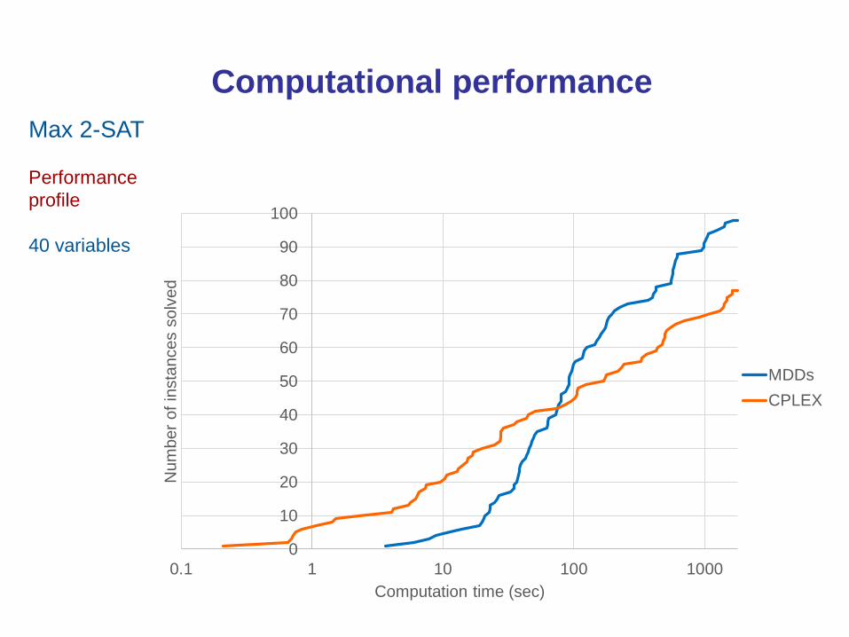
Max 2-SAT
Performance
profile
40 variables
0
10
20
30
40
50
60
70
80
90
100
0.1 1 10 100 1000
Num
ber
of
insta
nces s
olv
ed
Computation time (sec)
MDDs
CPLEX
Computational performance

● Potential to scale up
– No need to load large inequality model into solver.
– Parallelizes very effectively
– Near-linear speedup.
– Much better than mixed integer programming.
84
Computational performance

Computational performance
● In all computational comparisons so far…
– Problem is easily formulated for IP.
● DD-based optimization is most competitive when…
– Problem has a recursive dynamic programming model…
– and no convenient IP model.

Computational performance
● In all computational comparisons so far…
– Problem is easily formulated for IP.
● DD-based optimization is most competitive when…
– Problem has a recursive dynamic programming model…
– and no convenient IP model.
● Such as…
– Sequencing and scheduling problems (next talk)
– Planning problems
– DP problems with exponential state space
• New approach to “curse of dimensionality”
– Problems with nonconvex, nonseparable objective function…

● Weighted DD can represent any objective function
– Separable functions are the easiest, but any
nonseparable function is possible.
– Can be nonlinear, nonconvex, etc.
– The issue is complexity of resulting DD
87
Modeling the Objective Function

● Weighted DD can represent any objective function
– Separable functions are the easiest, but any
nonseparable function is possible.
– Can be nonlinear, nonconvex, etc.
– The issue is complexity of resulting DD
● Multiple encodings
– A given objective function can be encoded by multiple
assignments of costs to arcs.
– There is a unique canonical arc cost assignment.
– Which can reduce size of exact DD.
– Design state variables accordingly
88
Modeling the Objective Function
Modeling the Objective Function
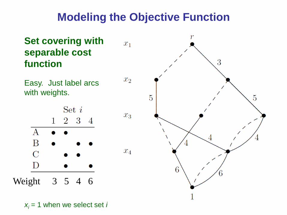
Set covering with
separable cost
function
Easy. Just label arcs
with weights.
xi = 1 when we select set i
Weight 3 5 4 6

Nonseparable cost
function
Now what?
Modeling the Objective Function

Nonseparable cost function
Put costs on leaves
of branching tree.
Modeling the Objective Function
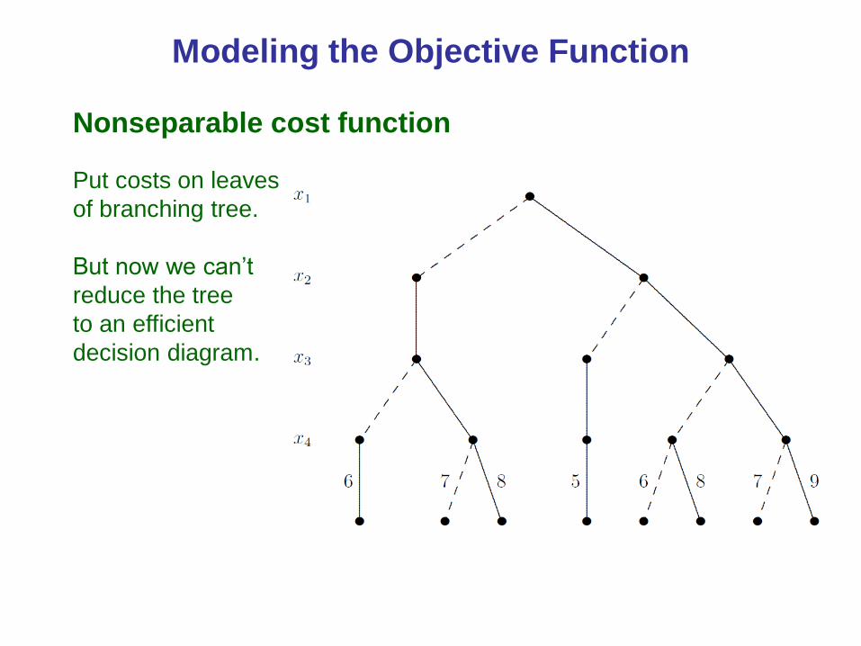
Nonseparable cost function
Put costs on leaves
of branching tree.
But now we can’t
reduce the tree
to an efficient
decision diagram.
Modeling the Objective Function

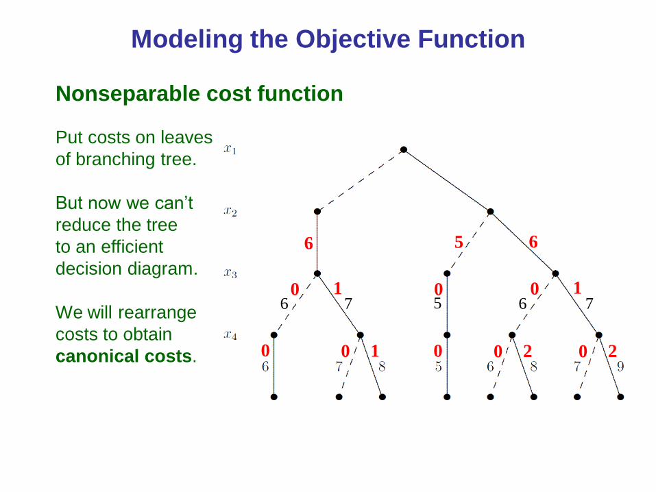
Nonseparable cost function
Put costs on leaves
of branching tree.
But now we can’t
reduce the tree
to an efficient
decision diagram.
We will rearrange
costs to obtain
canonical costs.
Modeling the Objective Function

Nonseparable cost function
Put costs on leaves
of branching tree.
But now we can’t
reduce the tree
to an efficient
decision diagram.
We will rearrange
costs to obtain
canonical costs. 0
6
0 1
7
0
5
0 2 0 2
6 7
Modeling the Objective Function
0
6
0 1
7
0
5
0 2 0 2
6 70 1
6
0 10
5 6
Modeling the Objective Function
Nonseparable cost function
Put costs on leaves
of branching tree.
But now we can’t
reduce the tree
to an efficient
decision diagram.
We will rearrange
costs to obtain
canonical costs.

0
6
0 1
7
0
5
0 2 0 2
6 70 1
6
0 10
5 60 0 1
6 5
Modeling the Objective Function
Nonseparable cost function
Put costs on leaves
of branching tree.
But now we can’t
reduce the tree
to an efficient
decision diagram.
We will rearrange
costs to obtain
canonical costs.

Nonseparable cost function
Now the tree can
be reduced.
0
6
0 1
7
0
5
0 2 0 2
6 70 1
6
0 10
5 60 0 1
6 5
Modeling the Objective Function

Nonseparable cost function
Now the tree can
be reduced.
Modeling the Objective Function
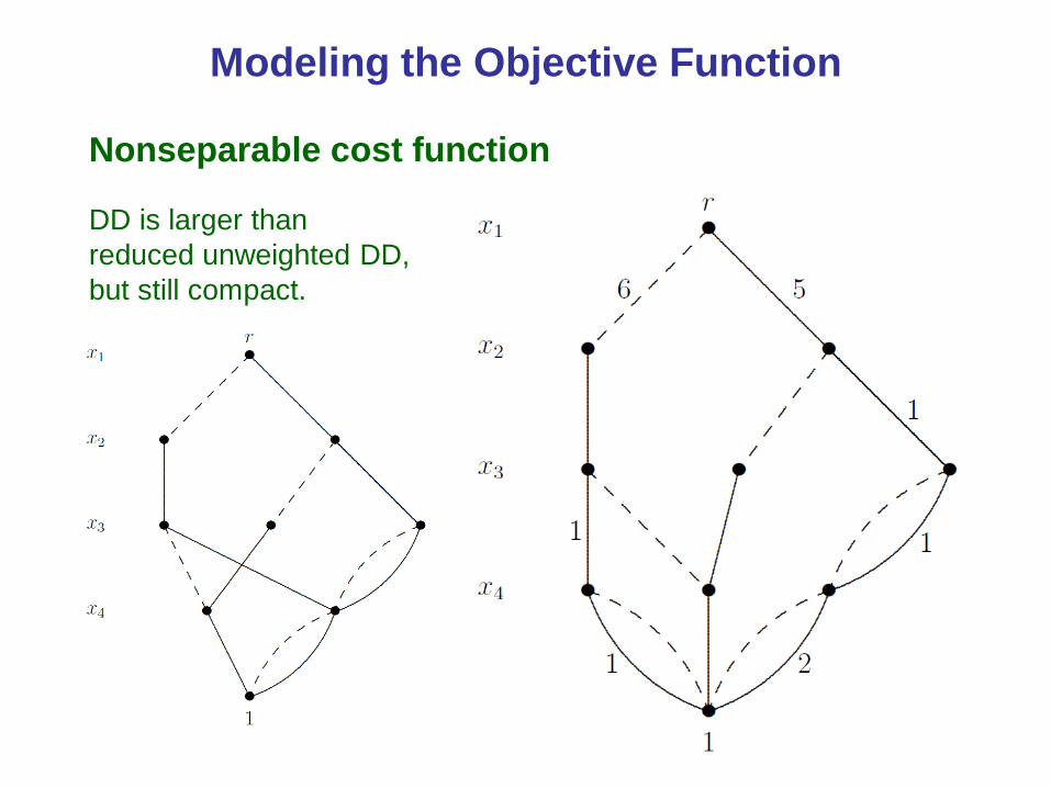
Nonseparable cost function
DD is larger than
reduced unweighted DD,
but still compact.
Modeling the Objective Function

Theorem. For a given variable ordering, a given
objective function is represented by a unique
weighted decision diagram with canonical costs.
Modeling the Objective Function
JH (2013),
Similar result for AADDs:
Sanner & McAllester (2005)

Inventory Management Example
● In each period i, we have:
– Demand di
– Unit production cost ci
– Warehouse space m
– Unit holding cost hi
● In each period, we decide:
– Production level xi
– Stock level si
● Objective:
– Meet demand each period while minimizing production and
holding costs.
2+5
1+15
4+3
2+9
0+6
0 21
0 21
0 21
0
0
0+8
0+60+4
0+12
0+9
0+10
0+20
0+15
4+6
4+0
2+10
2+0
4+0
0+12
2+3
2+6
1+5
1+10
2+6
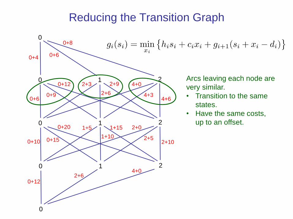
Arcs leaving each node are
very similar.
• Transition to the same
states.
• Have the same costs,
up to an offset.
Reducing the Transition Graph
0 21
0 21
0 21
0
0
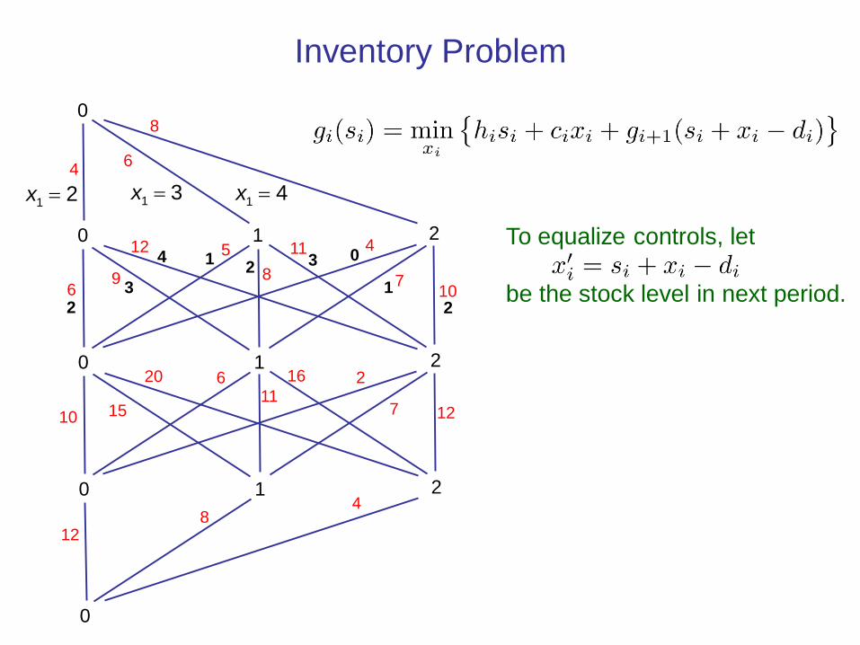
Inventory Problem
1 2x 1 3x 1 4x
To equalize controls, let
be the stock level in next period.
7
16
7
11
6
8
64
12
9
10
20
15
10
4
12
2
4
12
5
8
611
8
2
3
4 12 3 0
1
2

0 21
0 21
0 21
0
0
Inventory Problem
1 0x 1 1x 1 2x
To equalize controls, let
Be the stock level in next period.
7
16
7
11
6
8
64
12
9
10
20
15
10
4
12
2
4
12
5
8
611
8
0
1
2 01 2 0
1
2

7
16
7
11
6
0 21
0 21
0 21
0
0
8
64
12
9
10
20
15
10
4
12
2
4
12
5
8
611
8
Inventory Problem
1 0x 1 1x 1 2x
To equalize controls, let
Be the stock level in next period.0
1
2 01 2 0
1
2
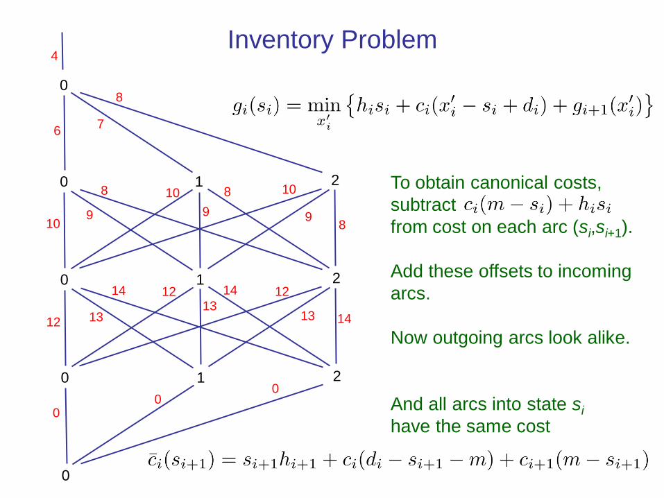
New recursion:

Inventory Problem
To obtain canonical costs,
subtract
from cost on each arc (si,si+1).
7
16
7
11
6
0 21
0 21
0 21
0
0
8
64
12
9
10
20
15
10
4
12
2
4
12
5
8
611
8

Inventory Problem
To obtain canonical costs,
subtract
from cost on each arc (si,si+1).
Add these offsets to incoming
arcs.5
10
3
6
0
0 21
0 21
0 21
0
0
4
20
6
3
0
10
5
6
0
10
0
4
0
0
3
05
0

Inventory Problem
To obtain canonical costs,
subtract
from cost on each arc (si,si+1).
Add these offsets to incoming
arcs.13
14
9
8
10
0 21
0 21
0 21
0
0
8
76
8
9
12
14
13
8
10
14
12
0
0
10
9
1213
0
4
Inventory Problem
To obtain canonical costs,
subtract
from cost on each arc (si,si+1).
Add these offsets to incoming
arcs.
Now outgoing arcs look alike.
And all arcs into state si
have the same cost
13
14
9
8
10
0 21
0 21
0 21
0
0
8
76
8
9
12
14
13
8
10
14
12
0
0
10
9
1213
0
4

Inventory Problem
These are canonical costs with
offset
13
14
9
8
10
0 21
0 21
0 21
0
0
8
76
8
9
12
14
13
8
10
14
12
0
0
10
9
1213
0
4

Inventory Problem
13
14
9
8
10
0 21
0 21
0 21
0
0
8
76
8
9
12
14
13
8
10
14
12
0
0
10
9
1213
0
4
These are canonical costs with
offset
New recursion:

Now there is only one state per period.
12
0
13 14
10 9 8
6 7 8
4
0
0
12
20
26
30
New recursion:
Inventory Problem
JH (2013)

Nonserial Decision Diagrams
● Analogous to nonserial dynamic programming,
independently(?) rediscovered many times:
– Nonserial DP (1972)
– Constraint satisfaction (1981)
– Data base queries (1983)
– k-trees (1985)
– Belief logics (1986)
– Bucket elimination (1987)
– Bayesian networks (1988)
– Pseudoboolean optimization (1990)
– Location analysis (1994)
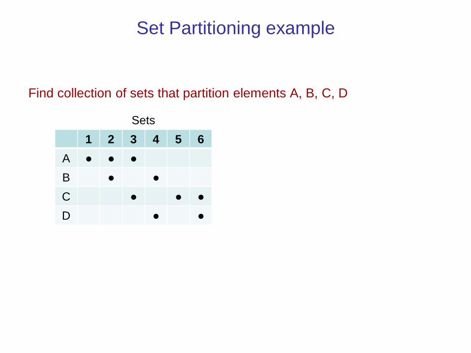
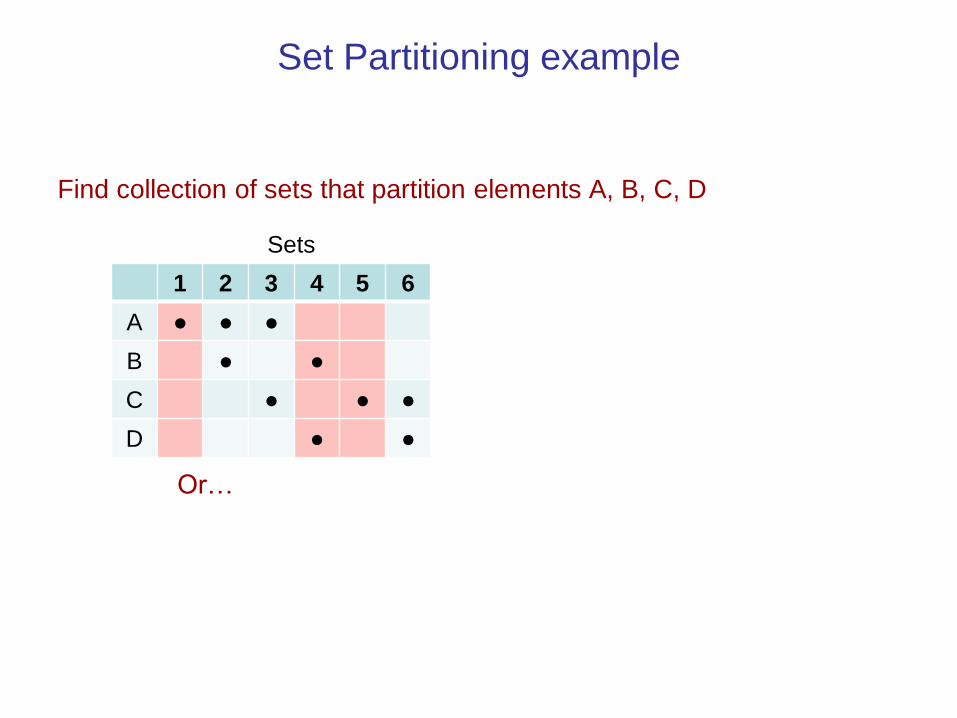
Set Partitioning example
Find collection of sets that partition elements A, B, C, D
1 2 3 4 5 6
A ● ● ●
B ● ●
C ● ● ●
D ● ●
Sets

Set Partitioning example
Find collection of sets that partition elements A, B, C, D
1 2 3 4 5 6
A ● ● ●
B ● ●
C ● ● ●
D ● ●
Sets
For example…
Set Partitioning example
Find collection of sets that partition elements A, B, C, D
1 2 3 4 5 6
A ● ● ●
B ● ●
C ● ● ●
D ● ●
Sets
Or…

Set Partitioning example
Find collection of sets that partition elements A, B, C, D
1 2 3 4 5 6
A ● ● ●
B ● ●
C ● ● ●
D ● ●
Sets
1 2 3
2 4
3 5 6
4 6
1
1
1
1
x x x
x x
x x x
x x
0-1 formulation
1 set selectedjx j

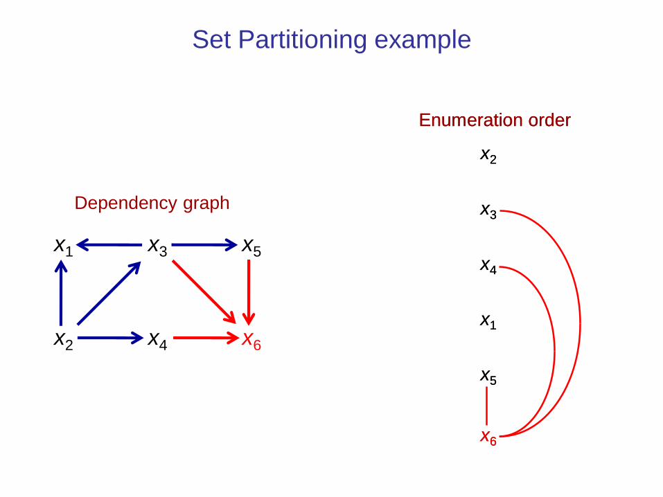
Set Partitioning example
Dependency graph
1 2 3
2 4
3 5 6
4 6
1
1
1
1
x x x
x x
x x x
x x
0-1 formulation
1 set selectedjx j
x1
x2
x3
x4
x5
x6

Set Partitioning example
Dependency graph
x1
x2
x3
x4
x5
x6
Enumeration order
x2
x3
x4
x5
x1
x6
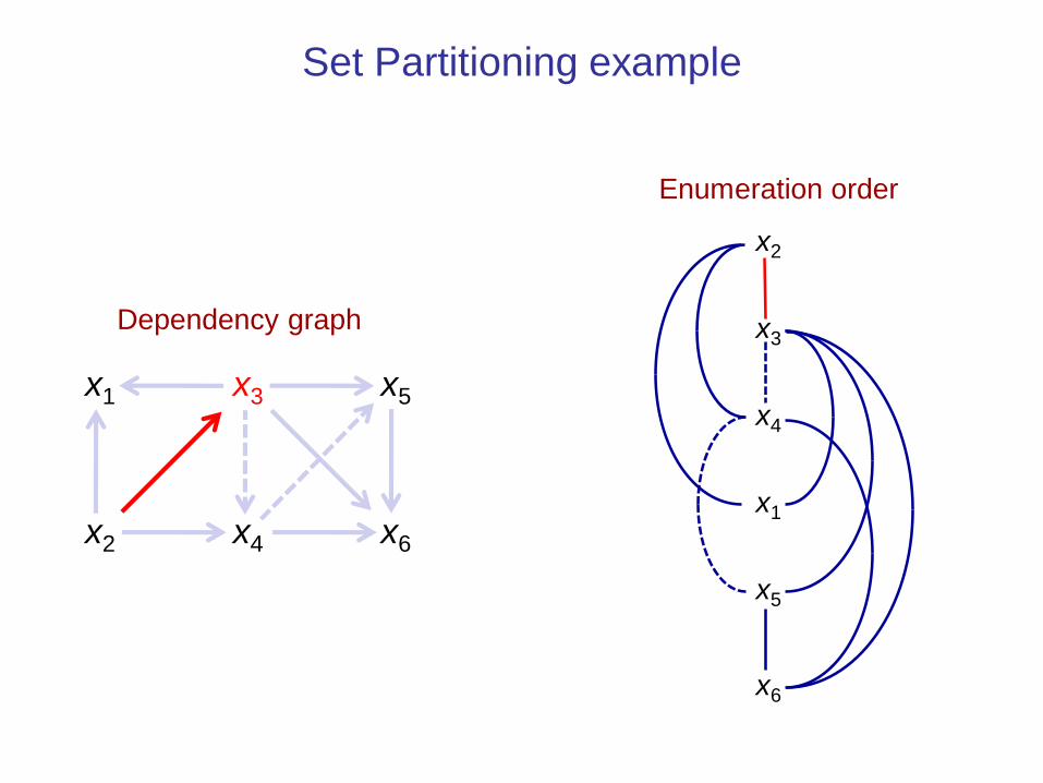
Set Partitioning example
Dependency graph
x1
x2
x3
x4
x5
x6
Enumeration order
x2
x3
x4
x5
x1
x6
Enumeration order
x2
x3
x4
x5
x1
x6

Set Partitioning example
Dependency graph
x1
x2
x3
x4
x5
x6
Enumeration order
x2
x3
x4
x5
x1
x6
Enumeration order
x2
x3
x4
x5
x1
x6

Set Partitioning example
Enumeration order
x2
x3
x4
x5
x1
x6
Dependency graph
x1
x2
x3
x4
x5
x6

Set Partitioning example
Dependency graph
x1
x2
x3
x4
x5
x6
Enumeration order
x2
x3
x4
x5
x1
x6

Set Partitioning example
Dependency graph
x1
x2
x3
x4
x5
x6
Enumeration order
x2
x3
x4
x5
x1
x6
Enumeration order
x2
x3
x4
x5
x1
x6
Set Partitioning example
Enumeration order
x2
x3
x4
x5
x1
x6
Dependency graph
x1
x2
x3
x4
x5
x6

Set Partitioning example
Dependency graph
x1
x2
x3
x4
x5
x6
Induced width = 3
(max in-degree)
Enumeration order
x2
x3
x4
x5
x1
x6

Set Partitioning example
Enumeration order
x2
x3
x4
x5
x1
x6
Solution by nonserial DP
x20 1
x2x3 00 01 10
x3x4 01 11
x1
x3x4x5 010 011 110 000 001
x6 0 1
00
1 0

Set Partitioning example
1 2 3 4 5 6
A ● ● ●
B ● ●
C ● ● ●
D ● ●
Sets
Solution by nonserial DP
x20 1
x2x3 00 01 10
x3x4 01 11
x1
x3x4x5 010 011 110 000 001
x6 0 1
00
1 0

Set Partitioning example
1 2 3 4 5 6
A ● ● ●
B ● ●
C ● ● ●
D ● ●
Sets
1 0 0 1 1 0
Feasible solution
x20 1
x2x3 00 01 10
x3x4 01 11
x1
x3x4x5 010 011 110 000 001
x6 0 1
00
1 0

Set Partitioning example
1 2 3 4 5 6
A ● ● ●
B ● ●
C ● ● ●
D ● ●
Sets
1 0 0 1 1 0
0 0 1 1 0 0
Feasible solution
x20 1
x2x3 00 01 10
x3x4 01 11
x1
x3x4x5 010 011 110 000 001
x6 0 1
00
1 0

Set Partitioning example
1 2 3 4 5 6
A ● ● ●
B ● ●
C ● ● ●
D ● ●
Sets
1 0 0 1 1 0
0 0 1 1 0 0
0 1 0 0 0 1
Feasible solution
x20 1
x2x3 00 01 10
x3x4 01 11
x1
x3x4x5 010 011 110 000 001
x6 0 1
00
1 0

Set Partitioning example
Solution by nonserial DP
x20 1
x2x3 00 01 10
x3x4 01 11
x1
x3x4x5 010 011 110 000 001
x6 0 1
00
1 0
Serialized DP
0 1
00 01 10
001 011
010 011 110 000 001
0 1
100
1001 0011 0100
x3x3x4
x1x2x3x4
x3x4x5
x6
x2
x2x3
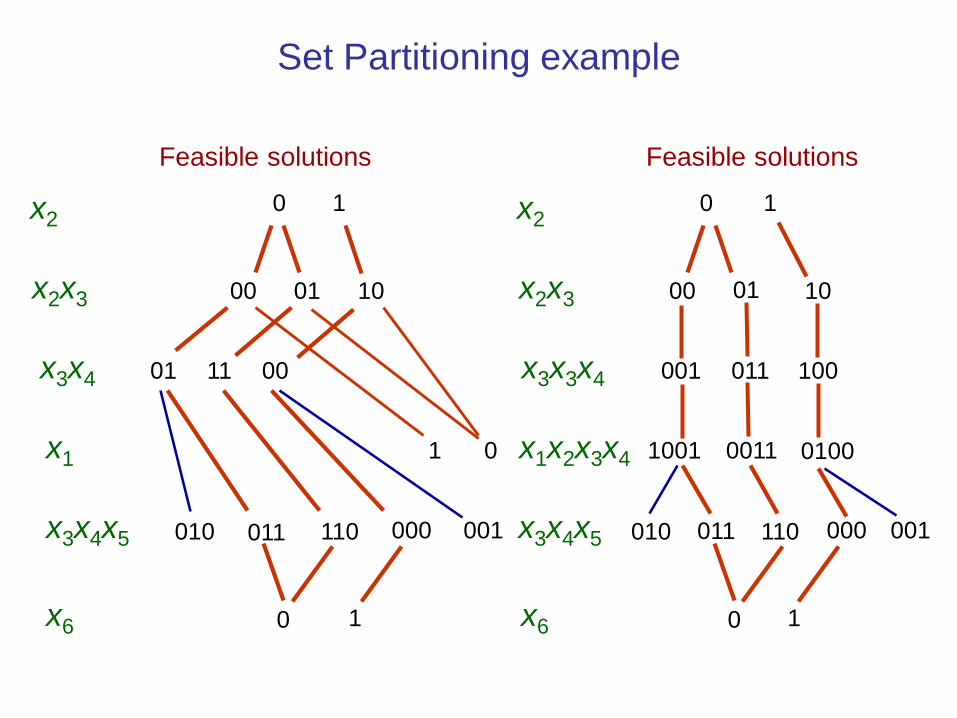
Set Partitioning example
Feasible solutions
x20 1
x2x3 00 01 10
x3x4 01 11
x1
x3x4x5 010 011 110 000 001
x6 0 1
00
1 0
Feasible solutions
0 1
00 01 10
001 011
010 011 110 000 001
0 1
100
1001 0011 0100
x3x3x4
x1x2x3x4
x3x4x5
x6
x2
x2x3

BDD vs. DP Solution
Serialized DP
0 1
00 01 10
001 011
010 011 110 000 001
0 1
100
1001 0011 0100
BDD
x20 1
x2x3 00 01 10
x3x4 001 011
x1
x3x4x5 011
110
000
x6 0
1
100
1001 0011 0100
x3x3x4
x1x2x3x4
x3x4x5
x6
x2
x2x3

BDD vs. DP Solution
Serialized DP
0 1
00 01 10
001 011
010 011 110 000 001
0 1
100
1001 0011 0100
BDD
x20 1
x2x3 00 01 10
x3x4 001 011
x1
x3x4x5 011
110
000
x6 0
1
100
1001 0011 0100
Deleted
x3x3x4
x1x2x3x4
x3x4x5
x6
x2
x2x3

BDD vs. DP Solution
Serialized DP
x20 1
x2x3 00 01 10
x3x3x4 001 011
x1x2x3x4
x3x4x5 010 011 110 000 001
x6 0 1
100
1001 0011 0100
BDD
x20 1
x2x3 00 01 10
x3x4 001 011
x1
x3x4x5 011
110
000
x6 0
1
100
1001 0011 0100
Merged

Set Partitioning example
Solution by nonserial DP
x20 1
x2x3 00 01 10
x3x4 01 11
x1
x3x4x5 010 011 110 000 001
x6 0 1
00
1 0

Set Partitioning example
Solution by nonserial DP
0 1
00 01 10
01 11
010 011 110 000 001
0 1
00
1 0
Nonserial BDD
x2 0 1
x2x3 00 01 10
x3x4 01 11
x1
x3x4x5011
110000
x60
1
00
0
1
x2
x2x3
x3x4
x1
x3x4x5
x6

Constructing the Join Tree
Clique in the
dependency graph
x1
x2
x3
x4
x5
x6
x1x2x3
x2 x3 x4 x1 x5 x6
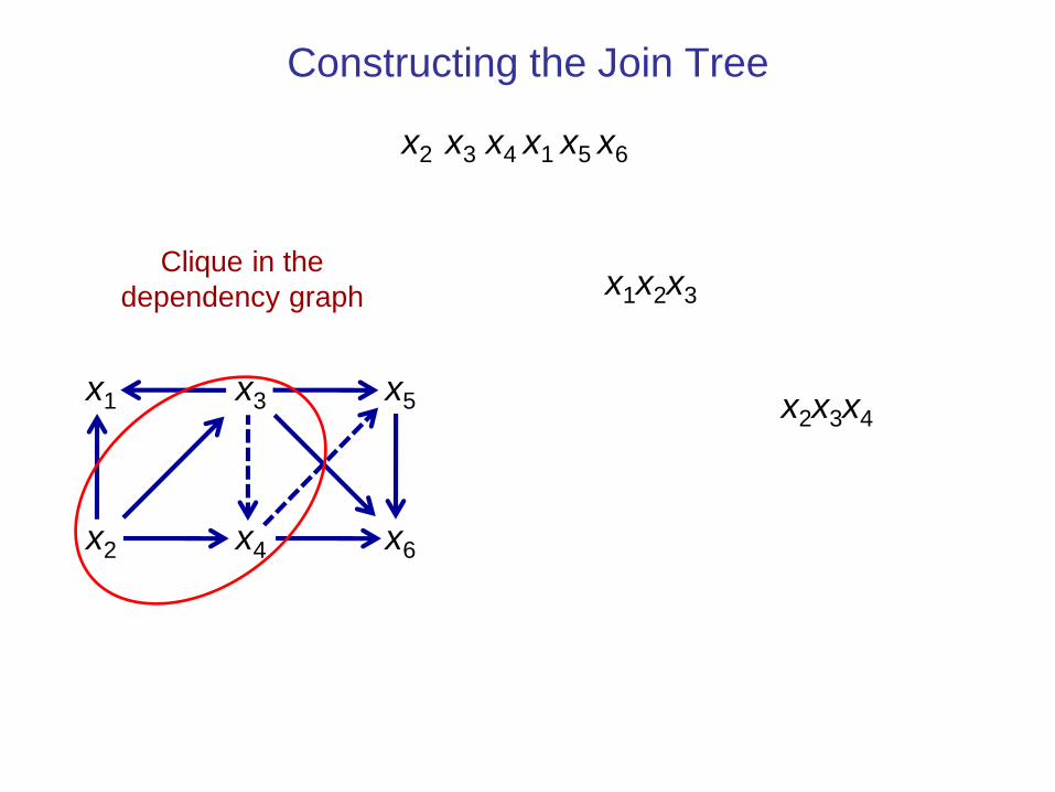
Constructing the Join Tree
x1
x2
x3
x4
x5
x6
x1x2x3
x2x3x4
Clique in the
dependency graph
x2 x3 x4 x1 x5 x6
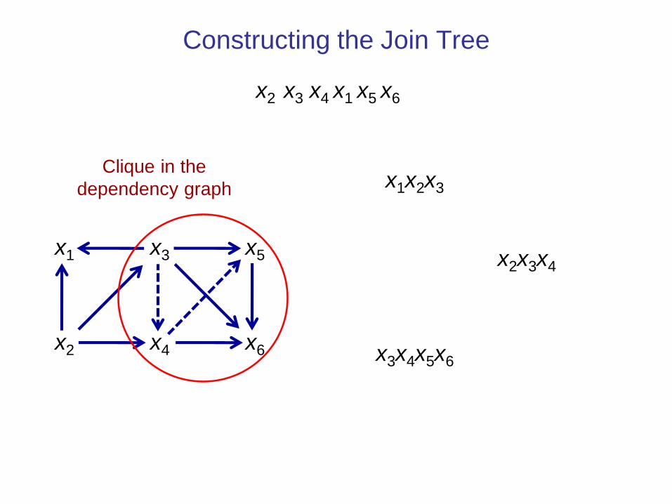
Constructing the Join Tree
x1
x2
x3
x4
x5
x6
x1x2x3
x2x3x4
x3x4x5x6
Clique in the
dependency graph
x2 x3 x4 x1 x5 x6

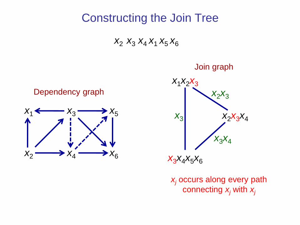
Constructing the Join Tree
x1
x2
x3
x4
x5
x6
x1x2x3
x2x3x4
x3x4x5x6
x3
x2x3
x3x4
Join graph
Connect nodes with
common variables
Dependency graph
x2 x3 x4 x1 x5 x6
Constructing the Join Tree
x1
x2
x3
x4
x5
x6
x1x2x3
x2x3x4
x3x4x5x6
x3
x2x3
x3x4
Join graph
xj occurs along every path
connecting xj with xj
Dependency graph
x2 x3 x4 x1 x5 x6

Constructing the Join Tree
x1
x2
x3
x4
x5
x6
x1x2x3
x2x3x4
x3x4x5x6
x3
x2x3
x3x4
Join graph
This can be viewed as the
constraint dual
Binary constraints equate common
variables in subproblems
Dependency graph
x2 x3 x4 x1 x5 x6

Constructing the Join Tree
Dependency graph
x1
x2
x3
x4
x5
x6
x1x2x3
x2x3x4
x3x4x5x6
x3
x2x3
x3x4
Join graph
Some edges may be redundant
when equating variables
x2 x3 x4 x1 x5 x6

Constructing the Join Tree
Dependency graph
x1
x2
x3
x4
x5
x6
x1x2x3
x2x3x4
x3x4x5x6
x2x3
x3x4
Join tree
Removing redundant edges
yields join tree
x2 x3 x4 x1 x5 x6
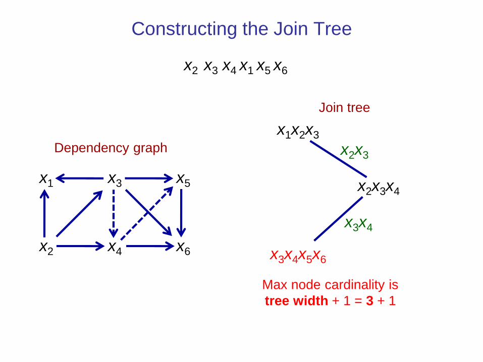
Constructing the Join Tree
Dependency graph
x1
x2
x3
x4
x5
x6
x1x2x3
x2x3x4
x3x4x5x6
x2x3
x3x4
Join tree
Max node cardinality is
tree width + 1 = 3 + 1
x2 x3 x4 x1 x5 x6

Constructing the Join Tree
Dependency graph
x1
x2
x3
x4
x5
x6
x1x2x3
x2x3x4
x3x4x5x6
x2x3
x3x4
Join tree
Induced width = tree width = 3
x2 x3 x4 x1 x5 x6

Designing the Nonserial BDD
x2x3x1
x2x3x4
x3x4x5x6
x2x3
x3x4
Join tree
x2 x3 x4 x1 x5 x6
x2
BDD design

Designing the Nonserial BDD
x2x3x1
x2x3x4
x3x4x5x6
x2x3
x3x4
Join tree
x2 x3 x4 x1 x5 x6
x2
x2x3
BDD design

Designing the Nonserial BDD
x2x3x1
x2x3x4
x3x4x5x6
x2x3
x3x4
Join tree
x2 x3 x4 x1 x5 x6
x2
x2x3
x3x4
BDD design

Designing the Nonserial BDD
x2x3x1
x2x3x4
x3x4x5x6
x2x3
x3x4
Join tree
x2 x3 x4 x1 x5 x6
x2
x2x3
x1
BDD design
x3x4

Designing the Nonserial BDD
x2x3x1
x2x3x4
x3x4x5x6
x2x3
x3x4
Join tree
x2 x3 x4 x1 x5 x6
x2
x2x3
x3x4 x1
x5
BDD design

Designing the Nonserial BDD
x2x3x1
x2x3x4
x3x4x5x6
x2x3
x3x4
Join tree
x2 x3 x4 x1 x5 x6
x2
x2x3
x3x4 x1
x6
x3x4x5
BDD design

Designing the Nonserial BDD
x2 x3 x4 x1 x5 x6
x2
x2x3
x3x4 x1
x6
x3x4x5
Nonserial BDD
x2 0 1
x2x3 00 01 10
01 11
x1
x3x4x5011
110000
x60
1
00
0
1
x3x4
BDD design

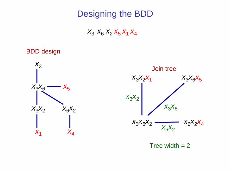
Another Variable Ordering
x1
x2
x3
x4
x5
x6
x3x2x1 x3x6x5
x3x6x2
x3x2
x3
x3x6
Join graph
Dependency graph
x3 x6 x2 x5 x1 x4
x6x2x4x6x2
x2
x6
Induced width = 2

Constructing the Join Tree
x1
x2
x3
x4
x5
x6
x3x2x1 x3x6x5
x3x6x2
x3x2
x3x6
Join treeDependency graph
x3 x6 x2 x5 x1 x4
x6x2x4x6x2
Induced width = 2 Tree width = 2

Designing the BDD
x3x2x1 x3x6x5
x3x6x2
x3x2
x3x6
Join tree
x3 x6 x2 x5 x1 x4
x6x2x4x6x2
Tree width = 2
x3
BDD design

Designing the BDD
x3x2x1 x3x6x5
x3x6x2
x3x2
x3x6
Join tree
x3 x6 x2 x5 x1 x4
x6x2x4x6x2
Tree width = 2
x3
x3x6
BDD design

Designing the BDD
x3x2x1 x3x6x5
x3x6x2
x3x2
x3x6
Join tree
x3 x6 x2 x5 x1 x4
x6x2x4x6x2
Tree width = 2
x3
x3x2
x3x6
x6x2
BDD design
Designing the BDD
x3x2x1 x3x6x5
x3x6x2
x3x2
x3x6
Join tree
x3 x6 x2 x5 x1 x4
x6x2x4x6x2
Tree width = 2
x3
x3x2
x3x6
x6x2
x5
x1 x4
BDD design

Nonserial BDD
x3 x6 x2 x5 x1 x4
x3
x3x2
x3x6
x6x2
x5
x1 x4
BDD design
Nonserial BDD
x3 0 1
x3x6 00 01 10
00
x10
1
01
10x2x3
0
1
x5
00 11
x2x6
x40
1

● Broader applicability
– Stochastic dynamic programming
– Continuous global optimization
● Combination with other techniques
– Lagrangean relaxation.
– Column generation
– Logic-based Benders decomposition
– Solve separation problem
163
Current Research
References
2006
• T. Hadzic and J. N. Hooker. Discrete global optimization with binary decision diagrams. In
Workshop on Global Optimization: Integrating Convexity, Optimization, Logic Programming,
and Computational Algebraic Geometry (GICOLAG), Vienna, 2006.
2007
• Tarik Hadzic and J. N. Hooker. Cost-bounded binary decision diagrams for 0-1
programming. In Proceedings of CPAIOR. LNCS 4510, pp. 84-98. Springer, 2007.
• Tarik Hadzic and J. N. Hooker. Postoptimality analysis for integer programming using binary
decision diagrams. December 2007, revised April 2008 (not submitted).
• M. Behle. Binary Decision Diagrams and Integer Programming. PhD thesis, Max Planck
Institute for Computer Science, 2007.
• H. R. Andersen, T. Hadzic, J. N. Hooker, and P. Tiedemann. A constraint store based on
multivalued decision diagrams. In Proceedings of CP. LNCS 4741, pp. 118-132. Springer,
2007.
2008
• T. Hadzic, J. N. Hooker, B. O'Sullivan, and P. Tiedemann. Approximate compilation of
constraints into multivalued decision diagrams. In Proceedings of CP. LNCS 5202, pp. 448-
462. Springer, 2008.
• T. Hadzic, J. N. Hooker, and P. Tiedemann. Propagating separable equalities in an MDD
store. In Proceedings of CPAIOR. LNCS 5015, pp. 318-322. Springer, 2008.

References
2010
• S. Hoda. Essays on Equilibrium Computation, MDD-based Constraint Programming and
Scheduling. PhD thesis, Carnegie Mellon University, 2010.
• S. Hoda, W.-J. van Hoeve, and J. N. Hooker. A Systematic Approach to MDD-Based
Constraint Programming. In Proceedings of CP. LNCS 6308, pp. 266-280. Springer, 2010.
• T. Hadzic, E. O’Mahony, B. O’Sullivan, and M. Sellmann. Enhanced inference for the
market split problem. In Proceedings, International Conference on Tools for AI (ICTAI),
pages 716–723. IEEE, 2009.
2011
• D. Bergman, W.-J. van Hoeve, and J. N. Hooker. Manipulating MDD Relaxations for
Combinatorial Optimization. In Proceedings of CPAIOR. LNCS 6697, pp. 20-35. Springer,
2011.
2012
• A. A. Cire and W.-J. van Hoeve. MDD Propagation for Disjunctive Scheduling. In
Proceedings of ICAPS, pp. 11-19. AAAI Press, 2012.
• D. Bergman, A.A. Cire, W.-J. van Hoeve, and J.N. Hooker. Variable Ordering for the
Application of BDDs to the Maximum Independent Set Problem. In Proceedings of CPAIOR.
LNCS 7298, pp. 34-49. Springer, 2012.

References
2013
• A. A. Cire and W.-J. van Hoeve. Multivalued Decision Diagrams for Sequencing Problems.
Operations Research 61(6): 1411-1428, 2013.
• D. Bergman. New Techniques for Discrete Optimization. PhD thesis, Carnegie Mellon
University, 2013.
• J. N. Hooker. Decision Diagrams and Dynamic Programming. In Proceedings of CPAIOR.
LNCS 7874, pp. 94-110. Springer, 2013.
• B. Kell and W.-J. van Hoeve. An MDD Approach to Multidimensional Bin Packing. In
Proceedings of CPAIOR, LNCS 7874, pp. 128-143. Springer, 2013.
2014
• D. R. Morrison, E. C. Sewell, S. H. Jacobson , Characteristics of the maximal independent
set ZDD, Journal of Combinatorial Optimization 28 (1) 121-139, 2014
• D. R. Morrison, E. C. Sewell, S. H. Jacobson, Solving the Pricing Problem in a Generic
Branch-and-Price Algorithm using Zero-Suppressed Binary Decision Diagrams,
• D. Bergman, A. A. Cire, W.-J. van Hoeve, and J. N. Hooker. Optimization Bounds from
Binary Decision Diagrams. INFORMS Journal on Computing 26(2): 253-258, 2014.
• A. A. Cire. Decision Diagrams for Optimization. PhD thesis, Carnegie Mellon University,
2014.
• D. Bergman, A. A. Cire, and W.-J. van Hoeve. MDD Propagation for Sequence Constraints.
JAIR, Volume 50, pages 697-722, 2014.
• D. Bergman, A. A. Cire, W.-J. van Hoeve, and T. Yunes. BDD-Based Heuristics for Binary
Optimization. Journal of Heuristics 20(2): 211-234, 2014.

References
2014
• D. Bergman, A. A. Cire, A. Sabharwal, H. Samulowitz, V. Saraswat, and W.-J. van Hoeve.
Parallel Combinatorial Optimization with Decision Diagrams. In Proceedings of CPAIOR,
LNCS 8451, pp. 351-367. Springer, 2014.
• A. A. Cire and J. N. Hooker. The Separation Problem for Binary Decision Diagrams. In
Proceedings of the International Symposium on Artificial Intelligence and Mathematics
(ISAIM), 2014. ]
2015
• D. Bergman, A. A. Cire, and W.-J. van Hoeve. Lagrangian Bounds from Decision Diagrams.
Constraints 20(3): 346-361, 2015.
• B. Kell, A. Sabharwal, and W.-J. van Hoeve. BDD-Guided Clause Generation. In
Proceedings of CPAIOR, 2015.
2016
• D. Bergman, A. A. Cire, W.-J. van Hoeve, and J. N. Hooker, Decision Diagrams for
Optimization, Springer, to appear.
• D. Bergman, A. A. Cire, W.-J. van Hoeve, and J. N. Hooker. Discrete Optimization with
Decision Diagrams. INFORMS Journal on Computing 28: 47-66, 2016.