Decentralized Multigrid for In-situ Big DataComputing

Abstract—Modern seismic sensors are capable of recordinghigh precision vibration data continuously for several months.Seismic raw data consists of information regarding earthquake’sorigin time, location, wave velocity, etc. Currently, these highvolume data are gathered manually from each station for analysis.This process restricts us from obtaining high-resolution imagesin real-time. A new in-network distributed method is requiredthat can obtain a high-resolution seismic tomography in realtime. In this paper, we present a distributed multigrid solutionto reconstruct seismic image over large dense networks. Thealgorithm performs in-network computation on large seismicsamples and avoids expensive data collection and centralizedcomputation. Our evaluation using synthetic data shows that theproposed method accelerates the convergence and reduces thenumber of messages exchanged. The distributed scheme balancesthe computation load and is also tolerant to severe packet loss.

Keywords—Distributed Multigrid, Cyber Physical System, BigData, Seismic Tomography, Sensor Network, In-network Computing

I. INTRODUCTION

Current volcano monitoring systems lack the capabilityof obtaining real time information and recover the physicaldynamics of seismic activity with sufficient resolution. Atpresent, the seismic tomography process involves aggregationof raw seismic data to centralized server for post-processingand analysis. To give some perspective on the volume, theraw seismic data are sampled with 16 − 24 bit precision at50−200Hz. These high fidelity samples are generally primary(p) or secondary (s) wave, that contains information such asearthquake origin time, location, wave velocity, etc. This highfrequency sampling at each node makes it extremely difficultto transmit the data over a dense sensor network due to severelimitations on energy and bandwidth. Due to these restrictions,many of the most threatening active volcanoes worldwideuse fewer than 20 nodes [26]. The existing scheme alsorequires months to generate satisfactory tomography images.This limits our ability to understand volcano dynamics andphysical processes in real-time. The centralized solution alsointroduces a bottleneck in computation. The risk of data lossalso increases in case of node failures, especially at the basestation. The centralized algorithm for these battery powerednodes, which have high risk of failures, are not suitable forvolcano monitoring.

The high volume raw samples consists of sparse earthquakeinformation, however current technology requires station totransfer all the raw samples of p and s wave to centralizedstation for post processing. In [29] the data collected from1980 - 2004 consists only of 19379 useful earthquake eventsand in addition 6916 events from october 2004 - december2005. Fig. 1 shows the parse distribution of earthquake eventsobtained from 78 station placed on Mt St Helens (MSH).

Few stations receive as few as 10 events while others receivemore than 900. This sparse feature of raw samples have ledresearchers to adopt distributed techniques to perform in-network processing and avoid centralized computation. Theadvancement in current wireless sensor technology makes itpossible to deploy and maintain a large-scale network forenvironmental monitoring and surveillance. However, seismictomography algorithms commonly in use today cannot beeasily implemented under this distributed scenario as it relieson centralized processing. Thus, real-time volcano tomographyrequires a practical approach which is distributed, scalable, andefficient with respect to tomography computation.

��

�

�

�

�

�

�

�

�

�

�

�

�

�

�

�

��

��

�

�

�

�

�

�

�

�

�

�

�

�

�

�

�

�

�

�

�

�

�

�

�

�

�

�

�

�

�

�

�

�

�

�

�

�

�

�

�

�

�

�

�

�

�

�

�

�

�

��

�

�

�

�

�

�

�

�

�

�

�

�

�

�

�

�

�

�

�

�

�

�

�

�

�

�

�

�

�

�

�

�

�

�

�

�

�

��

�

�

�

�

�

�

�

�

�

�

�

�

�

�

�

�

�

�

�

��

�

�

�

�

��

�

�

�

�

�

�

�

�

�

�

�

�

�

�

�

�

�

�

�

�

�

�

�

�

�

�

�

�

�

�

�

�

�

�

�

�

�

�

�

�

�

�

�

�

�

�

�

��

�

�

�

�

�

�

�

�

�

�

�

�

�

�

�

�

�

�

�

�

�

�

�

�

�

�

�

�

�

�

�

�

�

�

�

�

�

�

� �

�

�

�

�

�

�

�

�

�

�

�

�

�

�

�

�

�

�

�

�

�

�

�

�

�

�

�

�

�

�

�

�

�

�

�

�

�

�

�

�

�

�

�

�

�

�

�

�

�

�

�

�

��

��

�

�

�

�

�

�

�

�

�

�

�

�

�

�

�

�

�

�

�

�

�

�

�

�

�

�

�

�

�

�

�

�

�

�

�

�

�

�

�

�

�

�

�

�

�

�

�

�

�

�

�

�

�

�

�

�

�

�

��

�

�

�

�

��

�

�

�

�

�

�

�

�

�

�

��

�

��

��

�

��

�

�

�

�

�

�

�

�

�

�

�

�

�

�

�

�

�

�

�

�

�

�

�

�

�

�

�

�

�

�

�

�

�

�

�

�

�

�

��

�

�

�

� �

�

�

�

�

�

�

�

�

�

�

��

�

�

�

�

�

�

�

�

�

�

�

�

��

�

�

� �

�

�

�

�

�

�

�

�

�

�

�

�

�

�

�

�

�

�

�

�

�

�

�

�

�

�

�

�

�

�

�

��

�

�

�

�

�

�

�

�

�

�

�

�

�

�

�

�

�

�

�

�

�

�

�

�

� �

�

�

�

�

�

�

�

�

�

�

�

�

�

�

�

�

�

�

�

��

�

�

�

�

��

�

�

�

�

��

�

�

�

�

��

�

�

�

�

�

�

�

�

�

�

�

�

�

�

�

�

�

� �

��

�

�

�

�

�

��

�

�

�

�

�

�

�

�

�

�

�

�

�

�

�

�

�

�

�

�

�

�

��

�

�

�

�

�

� �

�

�

�

�

�

�

�

�

�

�

�

�

�

�

��

��

�

���

�

�

�

�

�

�

�

�

�

�

�

�

�

�

�

�

�

�

�

�

�

�

�

�

�

�

�

��

�

�

�

�

�

�

�

�

�

�

��

�

�

�

�

�

�

�

�

�

�

�

�

�

�

�

�

�

�

�

�

�

�

��

�

�

�

�

�

��

�

��

�

�

�

�

�

�

��

�

�

�

�

�

�

�

�

�

�

�

�

��

�

�

�

�

�

�

���

�

�

�

�

�

�

�

�

�

��

�

�

�

�

�

�

�

�

�

�

�

��

�

�

�

�

�

�� �

�

�

�

�

�

�

�

�

�

�

�

�

�

�

�

��

�

�

�

��

�

�

�

�

�

�

�

�

�

�

�

�

�

�

�

�

��

��

�

�

�

�

�

�

�

�

�

�

�

�

�

�

�

�

�

�

�

��

�

�

�

�

�

�

�

�

�

��

�

�

�

�

�

�

�

�

�

�

�

�

�

�

�

�

�

�

�

�

�

�

�

�

��

�

�

���

�

�

�

�

�

�

�

�

�

�

�

�

�

�

� �

�

�

�

�

�

�

��

��

�

�

�

�

�

�

�

�

�

�

�

�

��

�

�

�

�

�

�

�

�

�

�

��

�

�

�

�

�

�

�

�

�

�

�

��

�

�

�

�

�

�

�

�

�

�

�

�

�

�

�

�

�

�

�

�

�� �

�

�

��

�

�

�

�

�

��

�

�

�

�

�

�

�

�

�

�

�

�

�

�

�

�

�

�

�

�

�

�

�

�

�

�

�

�

�

�

�

�

�

�

�

�

�

�

�

�

�

�

�

�

��

�

�

�

�

�

�

�

�

�

�

�

��

�

�

�

�

��

�

�

� �

��

�

�

�

�

�

�

�

�

�

��

�

�

�

�

�

�

�

� �

�

�

�

�

�

��

�

�

�

�

�

�

�

�

�

�

�

�

�

�

�� �

�

�

�

�

�

�

�

�

�

�

�

�

�

�

�

�

�

�

�

�

�

�

�

�

�

�

�

��

�

�

� �

�

�

�

�

�

�

�

�

�

�

�

�

�

��

��

�

� �

�

�

�

�

�

�

�

60 70 80 90

3020

100

−10

X

Dept

h

(a) Earthquake Locations

0 10 20 30 40 50 60 70 800

200

400

600

800

1000

No.

of E

arth

quak

s

Station ID

(b) Event detection distribution

Fig. 1. Non-uniform distribution of rays and events at Mt St Helens.

Seismic tomography can be broadly classified into twomain categories: active and passive tomography. In active seis-mic tomography, earths interior is studied by sending p-wavesignal through external source such as vibrator, however inpassive tomography, measurements are taken based on p-wavegenerated by natural sources such as earthquake. Since late70’s active tomographic inversion of 2D and 3D structures havebeen studied widely both theoretically and also experimentallyby applying it to oil field exploration and volcanoes [13].Only in recent years, passive seismic tomography has beenstudied and the data obtained from few tens of nodes are beingused to study seismic activities. As mentioned earlier theseinversion methods rely on centralized data gathering schemeand has been implemented on volcanoes such as Mount St.Helens [17], Mount Rainier [19] as well as many others. Theresolution of such inversions are typically in tens of km’sand higher resolutions are hard to obtain from the existingsystems as the number of sensors are not sufficient to coverthe entire region of interest. Deploying large sensor nodesusing the current data gathering network is also not feasibleas these networks do not scale and sometimes it becomesimpossible due to data load. To overcome this, we developeda method called Component Average- Distributed Multiresolu-tion Evolving Tomography (CA-DMET) which computes thetomography over sensor networks [15]. In this method eachsensor nodes were responsible to calculate partial solution bysolving large sparse linear equation available to them using

2

Bayesian ART(BART) [18]. The partial solution obtained fromeach node was later combined with others to obtain thenext iterate. Convergence of this algorithm was proved to bebetter than other distributed methods. In this paper we try toaccelerate its convergence and improve the performance of thereconstruction using multigrid approach.

Typically when solving large sparse linear systems, it-erative methods tend to reduce high-frequency (oscillatory)components directly while not lower the errors caused due tolow-frequency. Multigrid methods are often used to mitigatethese low-frequency errors, as they reduce them by transferringthe problem to lower grids. We investigated our seismic to-mography inversion problem and found that multigrid could beused to accelerate the convergence. In this paper, we proposeDistributed MultiGrid Tomography (DMGT) algorithm whichaccelerates the convergence rate of CA-DMET. Our contribu-tion in the proposed approach differs from our previous algo-rithm CA-DMET in three ways: firstly we prove that BARTsatisfies the smoothing property and can be used as a smootherin multigrid. Secondly, we show that multigrid with BARTas smoother when applied on each node converge faster thanapplying only BART as used in CA-DMET. Thirdly, we showthat multigrid can be applied on each node distributedly andthe intermediate result can be combined using the componentaverage method. This paper mainly focuses on the distributedtomography algorithm, while assuming the arrival time ofevents at each node has been extracted from the raw seismicdata by each node itself [24], [27]. The algorithm proposedhere has application to fields far beyond the specifics ofvolcanology, e.g., oil field explorations have similar problemsand needs.

The rest of the paper is organized as follows. In section IIwe provide background on seismic tomography inversion andpresent the problem formulation. Section III presents relatedwork on distributed least squares, and distributed multigridmethods. In section IV we first discuss mathematical devel-opments that lead to the design of DMGT and then presentthe DMGT algorithm in detail. Simulation results are shownin section V. Finally we conclude the paper in section VI.

II. PROBLEM FORMULATION

Seismic Tomography: The methodology used in seismictomography is borrowed from medical tomography where thetravel time of elastic wave is used to probe internal structure.Although this idea is common in these two applications, thereare significant differences, mainly pertaining to size of thestructures and to event generation. The velocity model usedin seismic tomography is non-linear and the ray path of thewaves traveling through the ground may be highly curved dueto the size and complexity of the volcano. Typically, the raysource in volcano tomography is an earthquake event wherethe distribution of the ray path is highly non-uniform unlikeuniform short distance rays generated in medical imaging.These differences indicate that special care must be taken whentechniques borrowed from medical tomography are applied toseismic data.

The basic principle behind 2D or 3D seismic tomographyis to use the arrival time of the P-wave to derive the internal ve-locity structure of the volcano. This approach is called travel-time seismic tomography and the model here is continuously

evolving and refined as more earthquakes are recorded. Belowwe explain the three basic principles involved in travel-timeseismic tomography.

i) Event Location: Once an earthquake occurs, seismicdisturbances are detected by sensor nodes and arrival timesare recorded. Using these estimated arrival times, Geiger [8]introduced a technique to estimate the earthquake location andorigin time. This is a classic and widely used event localizationscheme generally using Gauss-Newton optimization.

ii) Ray Tracing: This is the technique of finding the raypaths from the seismic source locations to the sensor nodeswith minimum travel time. Given the source location of theseismic events and the current velocity mode of the volcano,ray tracing finds the ray paths from the event source locationto the nodes as shown in Fig. 2(b).

iii) Tomographic Inversion: The ray paths traced in turnare used to estimate the velocity model of the volcano. Thevolcano is partitioned into small blocks as shown in Fig. 2(c).This allows us to formulate the tomography problem as asystem of sparse linear equations. Suppose there are N sen-sor nodes and E earthquakes and x∗ denotes the referenceslowness (reciprocal of velocity) model of the volcano withresolution M blocks (eg. 32×32). Let x∗ denote the sum of x0,unperturbed model and x a small perturbation i.e., x∗ = x0+x.

Let b∗i = [b∗i1, b∗i2, · · · , b∗iE ]T , where b∗ie be the travel time

experienced by node i in the eth event. Based on the ray pathstraced in step (2), the travel time of a ray is the sum of theslowness in each block times the length of the ray within thatblock, i.e., b∗ie = Ai[e,m] ·x∗[m] where Ai[e,m] is the lengthof the ray from the eth event to node i in the mth block and x∗is the slowness of the mth block. Let b0i = [b0i1, b

0i2, · · · , b0iE ]T

be the unperturbed travel times where b0i = Ai[e,m] · x0[m].In the matrix notation we have following equation,

Aix∗ −Aix0 = Aix (1)

where Ai ∈ RE×M . Let bi = [bi1, bi2, · · · , biE ]T be the traveltime residual such that bi = b∗i − b0i , equation (1) can berewritten as,

Aix = bi (2)

Since each ray path intersects the model at a small number ofblocks, the design matrix, Ai, is sparse. For the system withN sensor nodes, the equation of the entire system would be,

Ax = B (3)

where B = [b1, b2, ....bN ]T , bi = [bi1, bi2, ....., biE ]T andA = [A1, A2, ....AN ]T .

Now from the above equation, each seismic sensor i ∈(1, · · · , N) contains at least E rows, i.e., earthquake eventsand travel time information. The column size of A denotes theresolution of the slowness model x being calculated. Our goalis to obtain the slowness model x without collecting the eventinformation from each node in a centralized server, but onlyby exchanging partial slowness between the sensors.

3

Earthquake

Event Location Ray Tracing Tomographic Inversion

Sensor Node

Seismic Wave

Estimated Magma Area

Blocks on Ray Path

Legends

Magma Magma

Earthquake

Estimated Event Location

Fig. 2. Procedures of Seismic Tomography Inversion

III. RELATED WORK

Distributed Linear Least Squares: The tomography in-version process mainly involve solving large sparse overdeter-mined systems of linear equations (3) and iterative methodsare commonly used. Several parallel and distributed iterativemethods have been developed and are currently being used tosolve a large variety of problems [11], [1]. Consensus basedmethods are the most widely used distributed algorithm forwireless sensor networks, e.g., [23]. These algorithms use aweighted sum of local estimates to achieve consensus. Eachsensor node maintains its own local estimation and exchangesinformation locally to achieve consensus. These methods areprimarily designed for estimation of low dimensional vec-tors typically in a parallel environment. To achieve globalconvergence, consensus protocols generally require relativelyhigh execution time and frequent communication betweenneighbors. In seismic tomography networks, this approach notonly means high communication overhead but also longerdelays involving many multi-hop communications. Therefore,the consensus-based distributed least square algorithms arenot suitable for high-resolution seismic tomography in sensornetworks.

Another method originally proposed for parallel computingis the multi-splitting solution of the least squares problem [22].This method partitions the system into columns instead ofrows, letting each processor compute a partial solution. Thesepartial solutions are exchanged iteratively to obtain globalconvergence. Column splitting of equation (3) in seismictomography means splitting the travel time ~B. Since we onlyhave the information of total travel time from event source tonode, we cannot divide ~B exactly and any heuristic approachwill add error in addition to existing system noise. Apart fromthat, this method is only linearly convergent and the communi-cation cost is very expensive as it requires exchanging ~B whichin our case increases with occurrences of earthquake events.Due to these reasons, column partitioning is not suitable forseismic tomography.

A popular iterative method for solving overdeterminedsystems was proposed by Kaczmarz (KACZ) [14] whichis an alternating projection method. This method is alsoknown under the name Algebraic Reconstruction Technique(ART) in computer tomography [12]. This algorithm doesnot require the full matrix to be in memory at one timeand can incorporate new information (ray paths), on the fly.The vectors of unknowns are updated after processing eachequation of the system and this cycle repeats until conver-gence. These iterative algorithms are distributed by averaging

the boundary information, e.g., Component Averaging (CAV)[4], Block Iterative-Component Averaging (BI-CAV) [3] andComponent-Averaged Row Projections (CARP) [9]. A surveypaper comparing various block parallel methods based ontheir performance on GPU’s is [7]. CA-DMET [15]involvedmodification of these algorithms for seismic tomography. Theconvergence of the iterative method used depended on spec-tral properties of the iteration matrix. Generally in iterativemethods, convergence stalls once the error is smooth i.e. high-frequency errors are reduced. Multigrid methods provide greattool to prevent stagnation by transferring smooth errors fromfine grids to coarse grids, resulting in overall acceleration ofconvergence [28], however, it cannot be applied to solve allthe problems arising from systems of linear equations [2].In this paper, we analyze the tomography problem carefullyand develop tools such as smoothers, intergrid operator etcsatisfying the requirements of multigrid.

Distributed Multigrid: Multigrid has been parallelized onmulticore computers and distributed memory clusters [30], [5].To perform multigrid in distributed networks, many new con-siderations arise, including high communication cost and thepossibility of packet loss. For example, some existing paralleland distributed multigrid algorithms partition the multigridlevels among different cores/nodes and the intergrid operatorscommunicate between each other to perform a multigrid cycle[25], [31]. In case of seismic tomography, exchanging the rowsof matrix A (ray information) between each nodes is expensiveand defeats the whole purpose of the distributed approach.Thus, we cannot adopt all previous techniques for parallelizingmultigrid and apply them to volcano tomography over sensornetworks.

Iterative methods such as Jacobi, Gauss-Seidel, and SORfor many problems have the property of smoothing the errorand are used as the “smoother” in multigrid methods [28].However, for solving overdetermined systems, it is more natu-ral to use Kaczmarz or ART as the smoother. This appears tobe first considered in [20], [16] for multigrid in medical imagetomography in a centralized setup. For inconsistent overde-teremined systems, Extended Kacmarz (KE) was introduced[21] which performs column operations at each iteration tomanipulate the right hand side of the linear equation. Howeverin our case, since information over sensors are split row wise,column operations over the entire network will add significantcommunication. In this paper we propose Distributed Multi-Grid Tomography (DMGT) which accelerates the convergenceof seismic tomography inversion over a network and balancesthe computation cost with reduced communication. DMGT

4

uses Bayesian ART (BART) as a smoother and we provethat BART satisfies the smoothing property. We also showthat DMGT is applicable to seismic tomography. To the bestof our knowledge, this work is the first attempt to distributethe multigrid computation of seismic tomography in sensornetworks.

IV. DISTRIBUTED ALGEBRAIC MULTIGRID FORTOMOGRAPHY

This section is divided into two sub-sections. In sub-section(A) we present mathematical developments and algorithmsetup, where we give the mathematical tools that are requiredfor designing the algorithm. Later in sub-section (B) we givea detailed explanation of the design of the DMGT algorithm.

A. Mathematical developments

1) Bayesian ART: The tomography inverse probleminvolves finding a solution x which satisfies equation(3). Typically, the seismic tomography equation is quasi-overdetermined, inconsistent and contains measurement noise.Therefore, we need to use some form of regularization to avoidstrong, undesired influence of small singular values dominatingthe solutions. This can be achieved by using a regularizationparameter for the least-squares solution xLS , i.e.,

xLS = arg maxx‖B −Ax‖2 + λ2‖x‖2 (4)

where λ is the trade-off parameter that regulates the relativeimportance we assign to models that predict the data versusmodels that have a characteristic, a priori variance.

A variant of ART called Bayesian ART (BART) can beused for solving equation (3) by minimizing equation (4).Suppose the system Ax = b is inconsistent, then we haveAx + y = b where y is chosen from any given x. Thenthe system is transformed to a well-posed problem. Nowx and y can be solved simultaneously using the followingiterative algorithm [1], where ei is a unit vector with the ithcomponent equal to one, and λ is the regularization parameter.

Algorithm 1 Bayesian ART1: for k ← 0 until convergence or maximum number of iteration

do2: k ← i mod m +1

3: d(k) = ρ(k)λbi−(y

(k)i +λaTi ·x

(k))

1+λ2‖ai‖2

4: x(k+1) = x(k) + λd(k)ai5: y(k+1) = y(k) + d(k)ei6: end

Note that in the Bayesian ART method, we need anadditional vector y of length E, but in the kth step only onecomponent of r(k) needs to be updated. This method has beenused for seismic imaging in [18].

2) Multigrid: Multigrid methods are among the most effi-cient methods for solving the very large sparse system of linearequations [28], [2]. The core idea of multigrid is to reducethe error via transferring the problem between multiple levelsand solving them over these levels. The residual equation istransferred to coarser grids and its solution is used to correct

the finer resolution solution. This is performed recursively untilconvergence is met. The idea of multigrid aligns with multi-resolution techniques and we have shown in [15] that multi-resolution is essential in estimating volcano tomography.

The main components of multigrid are the smoother, pro-longation and restriction operators, and wide variety of theseare used in different scenarios. These components are chosenbased on the type of the problem to optimize convergence.Prolongation and restriction operators mainly decide the con-struction of finer and coarser grids. In case of tomography thegrids are constructed based on the principle of ray tracing andhere we will show that ray tracing can be used for prolongationand restriction in multigrid. Prolongation and restriction aregenerally termed as intergrid operators as they define thetransfer process between the grids. As mentioned earlier, thetomography problem has a geometric structure and here weexploit this structure to define the intergrid operators. However,these intergrid operators must have certain properties and inthis section we will show that our ray tracing satisfies theseproperties.

P1 P2

P5

P9

P13

P6

P14

P10

P3

P7

P11

P15

P4

P8

P12

P16

PH1 PH

2

PH3 PH

4

(a) Fine Grid

Pj1

Pj3 Pj4

Pj2

PHj

ray i { {{

Aij1

Aij2

Aij4

(Ap)ij

(b) Coarse Grid

Fig. 3. Relation between fine and coarse grid

Let n be the number of columns in A and suppose thatn = 4p and let P1, · · · , Pn be the pixels on the fine grid. Thecoarse grid is obtained by combining its 4 adjacent pixels ofthe fine grid as shown in Fig 3(a). Let S(j), j ∈ 1, · · · , p bethe set of indices of the fine grid that form the coarse gridPHj . i.e.,

S(j) = {j1, j2, j3, j4} ∀j = 1, · · · , p

wherej1 < j2 < j3 < j4

such that

PHj = {Pj1 ∪ Pj2 ∪ Pj3 ∪ Pj4}

From the above equation the coarse grid matrix Ap will be

Aijp =∑

k∈S(j)

Aik,∀i = {1, · · · ,m} j = {1, · · · , p} (5)

Now the interpolation operator Inp is given by

Inp =

{1 if i ∈ S(j)0 if i /∈ S(j)

(6)

5

We now see that A = Ap × Inp satisfying the interpolationproperty. We also observe that Inp has full column rank.

Remark 1. Notice that the interpolation operator only in-creases the number of columns in matrix A. We can alsoconsider a similar operator which also reduces the rows byweighting them, however this is beyond the scope of this paper.

Remark 2. The above multigrid operators are designed for 2Dcases, however 3D case can be easily derived using n = 8pi.e. cuboid.

We have now shown that the interpolation operator formedby using the property of ray tracing can be used as an intergridoperator in multigrid. We also saw that Bayesian ART (BART)can be used for solving tomography problems. Next we showhow BART can act as a smoother and prove it satisfies thesmoothing property of multigrid.

3) Bayesian ART as smoother: For seismic tomography,BART is commonly used rather than ART or Gauss-Seidel.The problem being inconsistent and ill-posed, BART outper-forms other standard iterative algorithms in terms of conver-gence and solution [18]. However, BART has not been provenas a smoother in a multigrid setup and in this section we willprove that BART satisfies the smoothing property.

Definition 1. The smoothing property is satisfied by therelaxation scheme if there exists a constant α > 0 (independentof size or eigenvalues of A) such that

‖e‖2A ≤ ‖e‖2A − α‖r‖2D−1 + ‖y‖2D−1 (7)

where, e = x − x∗ , r = Ae = Ax − b , e = x − x∗ , D =diag(A) , ‖x‖A =

√〈Ax, x〉 and ‖r‖D−1 =

√〈D−1r, r〉

With respect to the above definitions and notation, Theo-rem 6 in [20] shows that Kaczmarz relaxation for consistentsystems satisfies the following smoothing property

‖e‖2 ≤ ‖e‖2 − γ‖D 12 r‖2 (8)

where

D12 = diag(

1

‖A1‖2, · · · , 1

‖An‖2) (9)

γ =1

(1 + γ−(A))(1 + γ+(A))(10)

and

γ−(A) = max1≤i≤n

∑j≤i

|〈Ai, Aj〉|‖Ai‖2

; γ+(A) = max1≤i≤n

∑j≥i

|〈Ai, Aj〉|‖Ai‖2

Theorem 1. Bayesian ART (algorithm 1) as a relaxationscheme for inconsistent system (3) satisfies the smoothingproperty if there exists,

‖e‖2 ≤ ‖e‖2 − γ‖D 12 r‖2 + ‖D 1

2 y‖2 (11)

Proof: Shown in Appendix A

4) Three-Grid V Cycle: Here we describe the three-gridcorrection scheme used in our algorithm. If the finest resolutionof our system to solve is of dimension 32×32, then resolution16 × 16 is used as an intermediate grid and resolution 8 × 8the coarsest grid. The coarsest grid is solved directly as thedimension is small, however we can also solve it by certainsweeps/iteration of BART. Later, the fine grid correction stepis applied. The total number of iterations for one three-gridV-cycle will be equal to 4× l1. The three-grid V-cycle schemeis represented diagrammatically in Fig. 4.

Algorithm 2 vh ← V cycle(vh, bh)

1: vh = BART(Ah, bh, vh) % Relax using l1 sweeps of BART2: rh = bh −Ahvh % Compute fine-grid residual3: r2h = I2hh rh % Restrict the residual to coarse grid4: v2h = BART(A2h, r2h, 0)5: r4h = r2h −A2hv2h

6: r4h = I4h2hr2h

7: A4hu4h = r4h % Solve directly8: e4h = (A4h)−1r4h

9: e2h = I2h4he4h % Interpolate coarse grid error to fine grid

10: v2h = v2h + e2h % Correct the fine-grid approximation11: e2h = BART(A2h, b2h, v2h) % Relax using l1 sweeps of BART12: eh = Ih2he

2h

13: vh = vh + eh

14: vh = BART(Ah, bh, vh)

Fig. 4. V Cycle Scheme for three levels

B. Design of DMGT algorithm

In the previous sub-section, we discussed separately thecomponents of multigrid suitable for tomography. In this sub-section we will put these ideas together to design a distributedmultigrid scheme that can balance the computation load andcompute the least-square solution for seismic tomographyinversion over a sensor network. The seismic sensors aredeployed on top of the volcano and each sensor gathers rayinformation after detecting earthquake events and forms apartial set of linear equations. Later, each sensor performsDMGT locally to obtain the partial slowness model (xk) whichis then combined with the partial slowness model obtainedfrom other nodes using component averaging as shown inFig. 5 to obtain the next iterate (xk+1). This process isrepeated until it converges to a threshold after which weobtain the global slowness model (x). Here, we first showhow component averaging can be used to combine the partialslowness from each node to form the next iterate. Later wediscuss the working of distributed multigrid algorithm in detail.

Suppose there are N sensor nodes in the network and Eray paths are traced on each sensor node, following some

6

earthquake events. From section II the seismic tomographymodel will be of the form

Ax = B (12)

where B = [b1, b2, ....bN ]T , bi = [bi1, bi2, ....., biE ]T and A =[A1, A2, ....AN ]T .

Let the size of A be m×n, where√n denotes the resolution

we are calculating in case of 2-D. Let A1, A2 · · · , AN eachcontain m1,m2, · · · ,mE number of rows. Now in each node,we calculate the number of non-zero coefficients ∀j, where1 ≤ j ≤ n. Let Ij denote the index set of the blocks thatcontain an equation with a non-zero coefficient of xj . Let sj =|Ij | (size of Ij).

We first show how the partial slowness obtained fromeach node can be combined with others using an averag-ing lemma. Let A = A1,A2, . . . ,AN and xij denote thejth component of partial slowness obtained from ith node.The component averaging operator relative to A is transferoperator CAA : (Rn)N → (Rn) and defined as follows:Let x1, · · · , xN ∈ Rn be partial solution from all N sensornodes. Then CAA(x1, · · · , xN ) is the point in Rn whose jthcomponent is given by

CAA(x1, · · · , xN ) =1

sj

N∑t=1

xtj

Assume that for some 1 ≤ r ≤ n the partial slownessx1, · · · , xr are shared by two or more nodes i.e., s1, · · · , sr ≥2 and sr+1, · · · , sn = 1. For simplicity, denote y as thecomponents of Rs, and index vectors of Rs is given by:

y = (y1,1, · · · , ys,s1 , · · · , yr,1, · · · , yr,sr , yr+1, · · · , yn)

Now we map the space from E : Rn → Rs:

E(x1, .., xn) = (y1,1, .., ys,s1 , .., yr,1, .., yr,sr , yr+1, .., yn)

we can see from the above equation that (y1,1, · · · , ys,s1contains s1 elements, (yr,1, · · · , yr,sr ) contains sr elements.Now after taking averages component-wise, we have our newupdate as follows:

x1 =1

s1(y1,1 + · · ·+ ys,s1) ; xr =

1

sr(yr,1, · · · , yr,sr )

xr+1 = yr+1 ; xn = yn

Remark 3. We notice that, number of nodes N in componentaverage scheme theoretically has no upper limit and can bevery large. It should be noted that increasing N will increasethe communication cost to carry out the summation over thenetwork. This might also effect the rate of convergence and isshown in the simulation result.

Now we give the formal description of Distributed Multi-grid Tomography (DMGT) algorithm, see Algorithm [3].

Initialize line 1-4: Suppose there are N sensors and eachsensor initializes its ID and starting resolution d. Let Q = d×dbe the current tomography resolution where d is the initialresolution dimension. A slowness model xl of resolution Q isused as an initial guess for ray tracing.

Algorithm 3 Distributed Multigrid TomographyInitialize

1: Node ID id,2: Initialize the starting resolution dimension d3: Initialize the number of seismic sensors N4: Current resolution dimension Q = d× d5: Initial slowness model for ray tracing xl

Repeat1: Upon the detection of an event2: Trace the ray path ae for every node3: Upon the reception of ~ae and be at each node start performing4: calculation at each node5: For each 1 ≤ j ≤ Q, calculate sj6: Where sj = |Ij | = {1 ≤ t ≤ N |xj has nonzero7: coefficient in some equation of node N8: k ← 0, xk ← 09: while not converged do

10: In Every node t for 1 ≤ t ≤ N do in parallel11: xt ← V cycle(xk, bt)12: Aggregate the partial slowness xt

13: from all nodes and find the next iterate:

14: x(k+1)j =

{xtj if sj = 11sj

∑Nt=1 x

tj if sj > 1

15: Send x(k+1)j to all the node N

16: k ← k + 117: end while18: xl ← x(k−1)

19: Upon the convergence obtaining final xl

20: Update slowness model: x(l+1) = xl

21: TERMINATE

Repeat line 1-2: After the initialization, each node willperform specific tasks based on the event detection and mes-sage reception. Once an event is detected by some node, thenode will perform the ray tracing algorithm (assuming eachnode is aware of event location) and obtain the ray path. Theneach node will compute the ray information forming a set oflinear equation,

[A1,A2, . . . ,AN ] · [x1,x2, . . . ,xQ]T = [b1,b2, . . . ,bN ]

where rows in Ai represents the ray information in each node,bi represents the travel time residual of rays obtained by thatnode and xj denotes the slowness of the jth grid in a 2Dtomographic cube of dimension Q.

Repeat line 3-18: Once all nodes compute the ray informa-tion, a parameter sj for all 1 ≤ j ≤ Q is calculated by each ofthem. sj is the number of nodes which has nonzero coefficientof particular xj . Once sj is calculated, each node simulta-neously performs some finite number of Multigrid VCycle(algorithm 2.). The next iterate is determined by componentaveraging technique given by x

(k+1)j = 1

sj

∑Nt=1 x

tj . Here a

tree based aggregation protocol is used calculate the sum andbroadcast back x

(k+1)j to all the nodes. The updated x

(k+1)j

is used as an initial guess for the next iteration. A stoppingcriteria is used to stop distributed multigrid and the finalslowness is sent to all the sensor nodes.

Repeat line 19-21: Once a sensor node receives the finalslowness model xl from all N nodes it will update the previousslowness model x(l+1) = xl. The algorithm will TERMINATEif obtained result is satisfactory for the volcanologists to

7

interpret. Otherwise the process is repeated with x(l+1) as theslowness model to do ray tracing with same resolution or withhigher depending upon the quality needed.

C. Communication Cost

From the above algorithm we see that the actual commu-nication in the network occurs in line 12− 15 which involvesaggregation of partial slowness data of size n from all thenodes and then broadcast the component averaged result backto each node. The communication scheme is shown in Fig. 5.Let xi for 1 ≤ i ≤ N be the partial solution of node i. Let|xi| denote the size of xi given by n. Then the worst casecommunication cost involved would be N

∑i dim(xi) = Nn.

Similarly after calculation of the component average, eachnode needs to flood the information to all other nodes whichinvolves another Nn communication. Since this algorithmconverges after k iterations, the worst case communication costwill be 2knN .

Sensor Nodes

Cluster Head

Tree based aggregate

[x’]

[x’]

[x’] [x’]

[x’]

[x’]

[x’] [x’]

[x’] [x’] Partial Slowness

Fig. 5. Communication Pattern for component averaging

In case of centralized computation we need to transfer theinformation from all the nodes to centralized server. Let mbe average size of rows in each node, then the worst casecommunication cost involved for transferring data over thenetworks will be Nmn. The average events each node detectsi.e. m will be of the order thousands or tens of thousands.Moreover, m is not constant and increases with occurrence ofearthquake,therefore we see that m� 2k. Also, in line 12−15the communication involved is summation of partial slownessover the network and the size of xi i.e n remains constantand is cheaper than passing all the node information to a basestation. Moreover, in centralized scenario if a node close tobase station fail then lots of packets will be dropped makingreconstruction impossible. While node failure in distributedcase will only lead to loss of part of A and reconstruction isstill possible using A’s on remaining nodes.

V. EVALUATION AND VALIDATION

In this section, we evaluate the DMGT algorithm andpresent the simulation results. Typically, to test tomographyinversion algorithm a synthetic model is used. This serves twopurpose: a) the real data set such as from Mt. St Helens donot have a ground truth and it is still uncertain which modelis reliable. b) The simulation using synthetic model enables usto investigate individually various phenomena which cannot beseparated physically. For example, p-wave data always contain

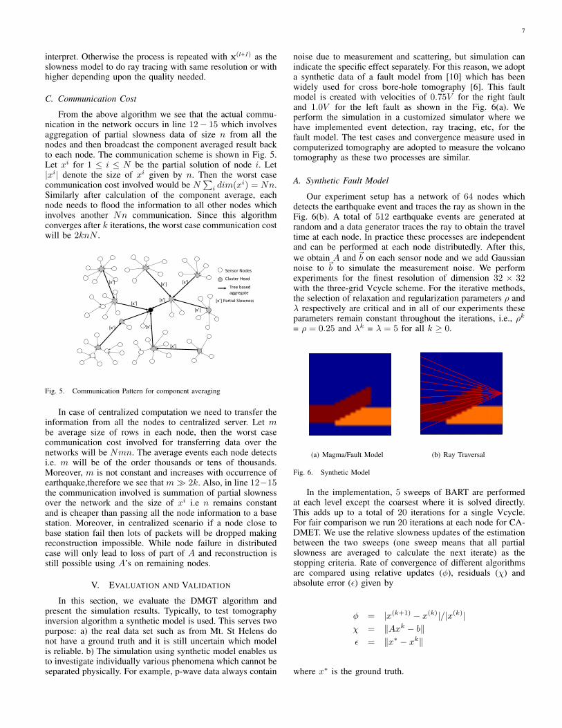
noise due to measurement and scattering, but simulation canindicate the specific effect separately. For this reason, we adopta synthetic data of a fault model from [10] which has beenwidely used for cross bore-hole tomography [6]. This faultmodel is created with velocities of 0.75V for the right faultand 1.0V for the left fault as shown in the Fig. 6(a). Weperform the simulation in a customized simulator where wehave implemented event detection, ray tracing, etc, for thefault model. The test cases and convergence measure used incomputerized tomography are adopted to measure the volcanotomography as these two processes are similar.

A. Synthetic Fault Model

Our experiment setup has a network of 64 nodes whichdetects the earthquake event and traces the ray as shown in theFig. 6(b). A total of 512 earthquake events are generated atrandom and a data generator traces the ray to obtain the traveltime at each node. In practice these processes are independentand can be performed at each node distributedly. After this,we obtain A and ~b on each sensor node and we add Gaussiannoise to ~b to simulate the measurement noise. We performexperiments for the finest resolution of dimension 32 × 32with the three-grid Vcycle scheme. For the iterative methods,the selection of relaxation and regularization parameters ρ andλ respectively are critical and in all of our experiments theseparameters remain constant throughout the iterations, i.e., ρk= ρ = 0.25 and λk = λ = 5 for all k ≥ 0.

(a) Magma/Fault Model (b) Ray Traversal

Fig. 6. Synthetic Model

In the implementation, 5 sweeps of BART are performedat each level except the coarsest where it is solved directly.This adds up to a total of 20 iterations for a single Vcycle.For fair comparison we run 20 iterations at each node for CA-DMET. We use the relative slowness updates of the estimationbetween the two sweeps (one sweep means that all partialslowness are averaged to calculate the next iterate) as thestopping criteria. Rate of convergence of different algorithmsare compared using relative updates (φ), residuals (χ) andabsolute error (ε) given by

φ = |x(k+1) − x(k)|/|x(k)|χ = ‖Axk − b‖ε = ‖x∗ − xk‖

where x∗ is the ground truth.

8

TABLE I. ROBUSTNESS OF DMGT

Cases Relative Error (φ) Absolute Error (ε )No Packet Loss 0.0052 3.4606

10% Packet Loss 0.0386 3.528140% Packet Loss 0.0612 3.7411

B. Correctness and Accuracy

Firstly, we compare the relative performance of DMGTwith two different algorithms: CA-DMET and MG-ART [16].We use residuals and absolute error as the parameters forcomparison and results are shown in Fig. 7. These plotsdemonstrate that there is a difference in the initial convergencebehavior in these algorithms. Although the residuals of CA-DMET and MG-ART decrease at a similar rate, the absoluteerror of MG-ART tends to diverge from ground truth. Thisbehavior is due to the lack of regularization parameter in thisalgorithm to handle inconsistent systems, whereas BART inDMGT takes care of this using appropriate λ. The iterations onx-axis denote the number of component averages required overa network i.e k as discussed earlier. We can see that DMGTconverges faster (lesser k) compared to CA-DMET whichmeans it requires lesser communication over the network.

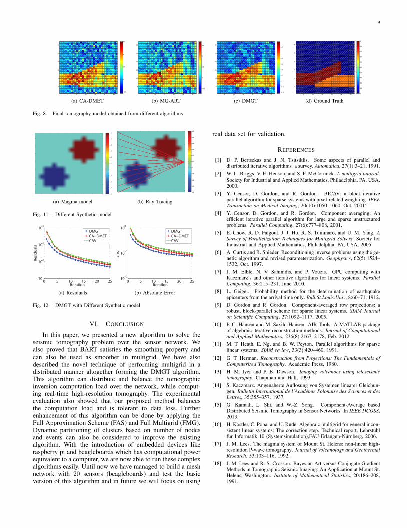
A visual verification of these three algorithms is shownin Fig. 8. All the algorithms are run for the same number ofiterations. The reconstructed images from different algorithmsreveal that DMGT is able to obtain better reconstructioncompared to other algorithms. We also observed that CA-DMET and DMGT algorithms continued to improve its imagereconstruction with further increase in iterations, however MG-ART’s reconstruction deteriorated with increase in iterations.This is also because of the inconsistent system as mentionedearlier.

5 10 15 20

102.1

102.5

Iteration

Residuals

CA-DMET

MG−ART

DMGT

(a) Residual

5 10 15 20

101

Iteration

Error

CA-DMET

MG−ART

DMGT

(b) Absolute Error

Fig. 7. Comparing CA-DMET, MG-ART and DMGT

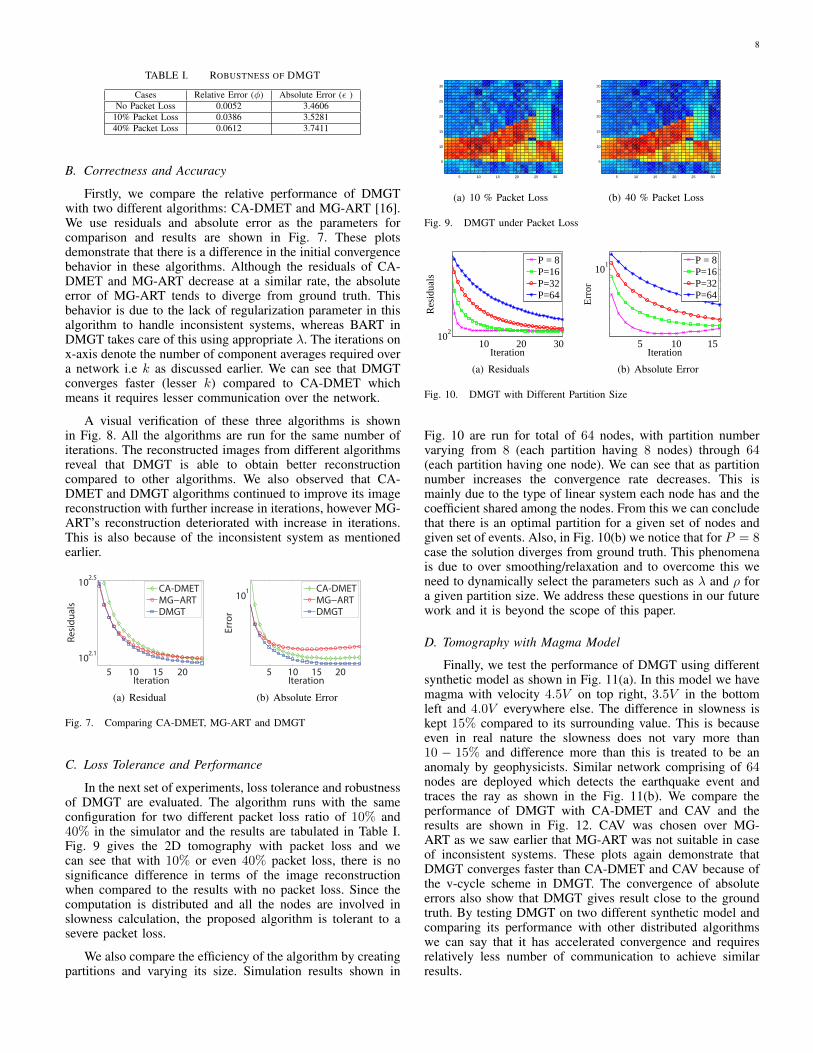
C. Loss Tolerance and Performance

In the next set of experiments, loss tolerance and robustnessof DMGT are evaluated. The algorithm runs with the sameconfiguration for two different packet loss ratio of 10% and40% in the simulator and the results are tabulated in Table I.Fig. 9 gives the 2D tomography with packet loss and wecan see that with 10% or even 40% packet loss, there is nosignificance difference in terms of the image reconstructionwhen compared to the results with no packet loss. Since thecomputation is distributed and all the nodes are involved inslowness calculation, the proposed algorithm is tolerant to asevere packet loss.

We also compare the efficiency of the algorithm by creatingpartitions and varying its size. Simulation results shown in

5 10 15 20 25 30

5

10

15

20

25

30

(a) 10 % Packet Loss

5 10 15 20 25 30

5

10

15

20

25

30

(b) 40 % Packet Loss

Fig. 9. DMGT under Packet Loss

10 20 3010

2

Iteration

Res

idua

ls

P = 8P=16P=32P=64

(a) Residuals

5 10 15

101

Iteration

Err

or

P = 8P=16P=32P=64

(b) Absolute Error

Fig. 10. DMGT with Different Partition Size

Fig. 10 are run for total of 64 nodes, with partition numbervarying from 8 (each partition having 8 nodes) through 64(each partition having one node). We can see that as partitionnumber increases the convergence rate decreases. This ismainly due to the type of linear system each node has and thecoefficient shared among the nodes. From this we can concludethat there is an optimal partition for a given set of nodes andgiven set of events. Also, in Fig. 10(b) we notice that for P = 8case the solution diverges from ground truth. This phenomenais due to over smoothing/relaxation and to overcome this weneed to dynamically select the parameters such as λ and ρ fora given partition size. We address these questions in our futurework and it is beyond the scope of this paper.

D. Tomography with Magma Model

Finally, we test the performance of DMGT using differentsynthetic model as shown in Fig. 11(a). In this model we havemagma with velocity 4.5V on top right, 3.5V in the bottomleft and 4.0V everywhere else. The difference in slowness iskept 15% compared to its surrounding value. This is becauseeven in real nature the slowness does not vary more than10 − 15% and difference more than this is treated to be ananomaly by geophysicists. Similar network comprising of 64nodes are deployed which detects the earthquake event andtraces the ray as shown in the Fig. 11(b). We compare theperformance of DMGT with CA-DMET and CAV and theresults are shown in Fig. 12. CAV was chosen over MG-ART as we saw earlier that MG-ART was not suitable in caseof inconsistent systems. These plots again demonstrate thatDMGT converges faster than CA-DMET and CAV because ofthe v-cycle scheme in DMGT. The convergence of absoluteerrors also show that DMGT gives result close to the groundtruth. By testing DMGT on two different synthetic model andcomparing its performance with other distributed algorithmswe can say that it has accelerated convergence and requiresrelatively less number of communication to achieve similarresults.

9

5 10 15 20 25 30

5

10

15

20

25

30

−0.5

0

0.5

1

1.5

(a) CA-DMET5 10 15 20 25 30

5

10

15

20

25

30

−0.5

0

0.5

1

1.5

(b) MG-ART5 10 15 20 25 30

5

10

15

20

25

30

−0.4

−0.2

0

0.2

0.4

0.6

0.8

1

1.2

(c) DMGT5 10 15 20 25 30

5

10

15

20

25

30

0

0.1

0.2

0.3

0.4

0.5

0.6

0.7

0.8

0.9

1

(d) Ground Truth

Fig. 8. Final tomography model obtained from different algorithms

3.6

3.7

3.8

3.9

4

4.1

4.2

4.3

4.4

4.5

4.6

(a) Magma model

3.6

3.7

3.8

3.9

4

4.1

4.2

4.3

4.4

4.5

4.6

(b) Ray Tracing

Fig. 11. Different Synthetic model

0 5 10 15 20 2510

1

102

103

104

Iteration

Residuals

DMGT

CA−DMET

CAV

(a) Residuals

0 5 10 15 20 2510

−2

10−1

100

Iteration

Error

DMGT

CA−DMET

CAV

(b) Absolute Error

Fig. 12. DMGT with Different Synthetic model

VI. CONCLUSION

In this paper, we presented a new algorithm to solve theseismic tomography problem over the sensor network. Wealso proved that BART satisfies the smoothing property andcan also be used as smoother in multigrid. We have alsodescribed the novel technique of performing multigrid in adistributed manner altogether forming the DMGT algorithm.This algorithm can distribute and balance the tomographicinversion computation load over the network, while comput-ing real-time high-resolution tomography. The experimentalevaluation also showed that our proposed method balancesthe computation load and is tolerant to data loss. Furtherenhancement of this algorithm can be done by applying theFull Approximation Scheme (FAS) and Full Multigrid (FMG).Dynamic partitioning of clusters based on number of nodesand events can also be considered to improve the existingalgorithm. With the introduction of embedded devices likeraspberry pi and beagleboards which has computational powerequivalent to a computer, we are now able to run these complexalgorithms easily. Until now we have managed to build a meshnetwork with 20 sensors (beagleboards) and test the basicversion of this algorithm and in future we will focus on using

real data set for validation.

REFERENCES

[1] D. P. Bertsekas and J. N. Tsitsiklis. Some aspects of parallel anddistributed iterative algorithms a survey. Automatica, 27(1):3–21, 1991.

[2] W. L. Briggs, V. E. Henson, and S. F. McCormick. A multigrid tutorial.Society for Industrial and Applied Mathematics, Philadelphia, PA, USA,2000.

[3] Y. Censor, D. Gordon, and R. Gordon. BICAV: a block-iterativeparallel algorithm for sparse systems with pixel-related weighting. IEEETransaction on Medical Imaging, 20(10):1050–1060, Oct. 2001‘.

[4] Y. Censor, D. Gordon, and R. Gordon. Component averaging: Anefficient iterative parallel algorithm for large and sparse unstructuredproblems. Parallel Computing, 27(6):777–808, 2001.

[5] E. Chow, R. D. Falgout, J. J. Hu, R. S. Tuminaro, and U. M. Yang. ASurvey of Parallelization Techniques for Multigrid Solvers. Society forIndustrial and Applied Mathematics, Philadelphia, PA, USA, 2005.

[6] A. Curtis and R. Snieder. Reconditioning inverse problems using the ge-netic algorithm and revised parameterization. Geophysics, 62(5):1524–1532, Oct. 1997.

[7] J. M. Elble, N. V. Sahinidis, and P. Vouzis. GPU computing withKaczmarz’s and other iterative algorithms for linear systems. ParallelComputing, 36:215–231, June 2010.

[8] L. Geiger. Probability method for the determination of earthquakeepicenters from the arrival time only. Bull.St.Louis.Univ, 8:60–71, 1912.

[9] D. Gordon and R. Gordon. Component-averaged row projections: arobust, block-parallel scheme for sparse linear systems. SIAM Journalon Scientific Computing, 27:1092–1117, 2005.

[10] P. C. Hansen and M. Saxild-Hansen. AIR Tools A MATLAB packageof algebraic iterative reconstruction methods. Journal of Computationaland Applied Mathematics, 236(8):2167–2178, Feb. 2012.

[11] M. T. Heath, E. Ng, and B. W. Peyton. Parallel algorithms for sparselinear systems. SIAM review, 33(3):420–460, 1991.

[12] G. T. Herman. Reconstruction from Projections: The Fundamentals ofComputerized Tomography. Academic Press, 1980.

[13] H. M. Iyer and P. B. Dawson. Imaging volcanoes using teleseismictomography. Chapman and Hall, 1993.

[14] S. Kaczmarz. Angenaherte Auflosung von Systemen linearer Gleichun-gen. Bulletin International de l’Academie Polonaise des Sciences et desLettres, 35:355–357, 1937.

[15] G. Kamath, L. Shi, and W.-Z. Song. Component-Average basedDistributed Seismic Tomography in Sensor Networks. In IEEE DCOSS,2013.

[16] H. Kostler, C. Popa, and U. Rude. Algebraic multigrid for general incon-sistent linear systems: The correction step. Technical report, Lehrstuhlfur Informatik 10 (Systemsimulation),FAU Erlangen-Nurnberg, 2006.

[17] J. M. Lees. The magma system of Mount St. Helens: non-linear high-resolution P-wave tomography. Journal of Volcanology and GeothermalResearch, 53:103–116, 1992.

[18] J. M. Lees and R. S. Crosson. Bayesian Art versus Conjugate GradientMethods in Tomographic Seismic Imaging: An Application at Mount St.Helens, Washington. Institute of Mathematical Statistics, 20:186–208,1991.

10

[19] S. C. Moran, J. M. Lees, and S. D. Malone. P wave crustal velocitystructure in the greater Mount Rainier area from local earthquaketomography. Journal of Geophysical Research, 104(B5):10775–10786,1999.

[20] C. Popa. Algebraic Multigrid Smoothing Property of Kaczmarz’s Relax-ation for General Rectangular Linear Systems. Electronic Transactionson Numerical Analysis, 29:150–162, 2008.

[21] C. Popa and R. Zdunek. Kaczmarz extended algorithm for tomographicimage reconstruction from limited-data. Mathematics and Computersin Simulation, 65:579–598, 2004.

[22] R. A. Renaut. A Parallel Multisplitting Solution of the Least SquaresProblem. Numerical Linear Algebra with Applications, 5(1):11–31,1998.

[23] I. D. Schizas, G. Mateos, and G. B. Giannakis. Distributed LMS forconsensus-based in-network adaptive processing. IEEE Transactions onSignal Processing, 57(6):2365–2382, 2009.

[24] R. Sleeman and T. van Eck. Robust automatic P-phase picking:an on-line implementation in the analysis of broadband seismogramrecordings. Physics of the Earth and Planetary Interiors, 113(1-4):265–275, 1999.

[25] B. Smith, P. Bjorstad, and W. Gropp. Domain Decomposition: ParallelMulti-level Methods for Elliptic Partial Differential Equations. Cam-bridge University Press, 1996.

[26] W.-Z. Song, R. Huang, M. Xu, A. Ma, B. Shirazi, and R. Lahusen.Air-dropped Sensor Network for Real-time High-fidelity Volcano Mon-itoring. In The 7th Annual International Conference on Mobile Systems,Applications and Services (MobiSys), June 2009.

[27] R. Tan, G. Xing, J. Chen, W. Song, and R. Huang. Quality-drivenVolcanic Earthquake Detection using Wireless Sensor Networks. InThe 31st IEEE Real-Time Systems Symposium (RTSS), San Diego, CA,USA, 2010.

[28] U. Trottenberg, C. Oosterlee, and A. Schuller. Multigrid. AcademicPress, San Diego, CA, 2001.

[29] G. P. Waite and S. C. Moranb. VP Structure of Mount St. Helens,Washington, USA, imaged with local earthquake tomography. Journalof Volcanology and Geothermal Research, 182(1-2):113–122, 2009.

[30] U. M. Yang. Parallel Algebraic Multigrid Methods - High PerformancePreconditioners, volume 51, pages 209–236. Springer-Verlag, 2006.

[31] H. Yserentant. On the multi-level splitting of finite element spaces.Numer. Math, 49:379–412, 1986.

APPENDIX APROOF OF THEOREM 1

Proof: From the previous notations we have:

ek = xk − s(x0), k = 1, 2, · · · , e = em

ek = x(k−1) + λρ(k−1)(λbi − (y

(k−1)i + λaTi x

(k−1)))ai1 + λ2‖ai‖2

− s(x0)

ek = e(k−1) − λ2ρ(k−1) rki1 + λ2‖ai‖2

ai −

λρ(k−1)y(k−1)i

1 + λ2‖ai‖2ai

‖ek‖2 = ‖ek−1 − λ2ρ(k−1) rk−1i

1 + λ2‖ai‖2ai‖2 +

|λρ(k−1)|2 y(k−1)i

1 + λ2‖ai‖2ai −

2〈e(k−1) − λ2ρ(k−1) r(k−1)i

1 + λ2‖ai‖2ai,

λρ(k−1)y(k−1)i

1 + λ2‖ai‖2ai〉

= ‖ek−1‖2 − 2〈e(k−1), λ2ρ(k−1) rk−1i

1 + λ2‖ai‖2ai〉

+(λ2ρ(k−1))2(r

(k−1)i )2

1 + λ2‖ai‖2a2i +

(λρ(k−1))2(y

(k−1)i )2

1 + λ2‖ai‖2a2i −

2〈e(k−1), λρ(k−1) y(k−1)i

1 + λ2‖ai‖2ai〉+

2〈λ2ρ(k−1) r(k−1)i

1 + λ2‖ai‖2ai, λρ

(k−1) y(k−1)i

1 + λ2‖ai‖2ai〉

= ‖ek−1‖2 − (λ2ρ(k−1))2(r

(k−1)i )2

1 + λ2‖ai‖2a2i +

(λρ(k−1))2(y

(k−1)i )2

1 + λ2‖ai‖2a2i

= ‖e(k−1)‖2 − ‖D 12λ2r

(k−1)i ‖2 + ‖D 1

2 y(k−1)i ‖2

where : D = diag(ρ(k−1)a

2i

1 + λ2‖ai‖2)

Since, ‖D 12 y

(k−1)i ‖2 ≥ 0 , from equation (8)

we know, ‖e‖2 ≤ ‖e‖2 − γ‖D 12 r‖2

Therefore

ek ≤ ‖e(k−1)‖2 − ‖D 12λ2r

(k−1)i ‖2 + ‖D 1

2 y(k−1)i ‖2

We have now shown that BART satisfies the smoothingproperty and can be used as smoother in multigrid to solvethe tomography problem.