This paper was written for the October 5-6, 1995 Conference on "Structural Adjustment Policies in the 1990s:1

Experience and Prospects" organized by the Institute of Developing Economies, Tokyo, Japan. We are indebted toElaine Zimmerman for research assistance. We would also like to thank Lant Pritchett and Phillip Swagel for kindlyproviding us with data and Evelyn Taylor for assistance in preparing the manuscript.

December 11, 1995

Accounting for Differences in Economic Growth1

Barry BosworthThe Brookings Institution

Susan M. Collins

The Brookings Institution and Georgetown University

Yu-chin ChenHarvard University

Accounting for Differences in Economic Growthby

Barry Bosworth, Susan M. Collins and Yu-chin Chen

Abstract

This paper uses a combination of growth accounting and regression analysis to examine economicgrowth experiences of 88 developing and industrial economies over the period 1960-1992. The decompositionshows that increases in total factor productivity (TFP) have been surprisingly small in developing countries,and that accumulation of physical and human capital account for most of the growth per worker. Thisreinforces a finding of some previous authors, but for a much larger sample of countries. Further, the fact thatcountries with high rates of factor accumulation do not have unusually high rates of TFP growth provides littlesupport for the new endogenous growth theories. Our analysis also uncovers significant difficulties with theuse of investment rates and school enrollment rates as proxies for capital accumulation, highlighting a reasonwhy some previous studies have understated the importance of accumulation.

Our regression results strongly support the growing consensus that stable, orthodox macroeconomicpolicy, combined with outward oriented trade policies foster economic growth. We explore the channelsthrough which determinants of growth operate. Among other findings, we show that larger budget deficitsslow growth through reducing capital accumulation, while real exchange rate volatility operates mainly throughslowing TFP growth. Outward orientation appears to work through both channels.

Introduction

The question of why rates of economic growth differ across nations has long been a subject of research

and policy debate. The last decade has witnessed the development of several theoretical ideas that attempt to

move beyond the neoclassical model with its emphasis on diminishing returns to factors, such as capital

accumulation, that might be influenced by government policies. At the policy level, a new consensus has

emerged that has replaced the old emphasis on inward-oriented growth policies. Today, developing countries

are urged to focus their attention on the maintenance of a stable macroeconomic environment and the adoption

of microeconomic policies that limit the role of government and give precedence to private agents in open,

liberalized markets. Particular emphasis is assigned to the removal of barriers to free economic interchange

between the domestic economy and international markets.

In recent years, there have also been a large number of empirical studies aimed at providing

evidentiary support for the policy advice and identifying the key features that distinguish countries with high

and low rates of economic growth. On some issues the empirical evidence has been weak and contradictory.

For example, there is little agreement on some of the most basic issues, such as the importance of capital

accumulation in the growth process.

A recent paper by King and Levine suggested that differences in the amount of capital per worker

account for only a small amount of the differences in national standards of living; and, while capital

accumulation is important, it is far from a dominant factor in the explanation of differences in rates of

2

King and Levine (1994).2

Alwyn Young (1994a and 1994b).3

economic growth over time. Their analysis is supportive of much of the new policy consensus in that it2

implies that countries can achieve high rates of growth through means other than the painful postponement

of consumption. Measures aimed at liberalizing markets, increasing the degree of interaction with the global

economy and reducing the scope of government can speed the process of catching up with the industrial

countries through increasing the efficiency with which capital and labor are employed, total factor productivity

growth.

Alwyn Young has disputed this view by showing that high rates of factor accumulation largely account

for the rapid growth of the East Asian economies. He finds that gains in total factor productivity have been3

very similar to those of other economies. This conclusion is challenging both to those who perceive large

efficiency gains from market liberalization, and to those who advance East Asia as evidence of the benefits

of government industrial policies aimed at planning the structural evolution of the economy. On the other

hand, most researchers would interpret the empirical studies of the link between stable macroeconomic policies

and economic growth, and the positive contribution of an open trade regime as relatively robust findings.

However, the channels through which these actions affect growth remain very unclear.

Much of the empirical research has been stimulated by the development of large multi-country

databases at the World Bank and the Penn World Table that make it possible to undertake cross-country

comparisons of economic growth and its relationship to various indicators of economic policy. The cross-

country studies have pursued three basic methods of empirical analysis. The first uses regression analysis to

estimate the parameters of an underlying common production function. These studies have a long history, but

much of the work was limited to a few industrial countries until recently because of a shortage of the required

data. The second approach is of more recent vintage, and, although it also relies on regression analysis, it takes

a more eclectic view of the growth process -- including in the regressions a wide range of conditioning

3

variables that might influence the growth process rather than focusing on estimates of the production function

per se. The third approach, growth accounting, eschews the regression approach in favor of a framework

which concentrates on dividing the sources of growth between the contribution of increases in the quantity of

the factor inputs and the efficiency with which they are used.

Each of these approaches has its uses, but none are free from problems. Regression analysis is often

used to estimate the relative role of the different factors, such as capital and labor, in the production process;

but there are major issues of simultaneity, measurement error, and the choice of a specific functional form that

generate considerable controversy. For many purposes, the use of each factor's share in total income is an

equally valid and more straight-forward means of measuring their relative importance. Finally, production

function estimation often relies upon very simple measures of changes in technology -- a time trend plus a

catch-up term, for example. Yet, there is an increasing emphasis on differences in the technological

component, total factor productivity, as critical to the explanation of differences in levels and rates of change

of income per capita across countries.

Today, the more common objective of the regression-based studies is to search for important

regularities in the data: examining the correlation between economic growth, initial conditions, and the role

of the government policy regime. These studies can be very useful in identifying important characteristics that

distinguish the high and low-growth economies, but the methodology is limited as a means of providing insight

into the channels through which the various factors operate. Thus, there is a substantial concern that the

empirical results may reflect spurious correlations or the common influence of other unidentified factors.

Growth accounting offers a more structured framework for assessing the role of various factors in the

growth process. It relies upon principles of cost minimization and marginal productivity analysis to use

earnings as the basis for developing a set of weights to combine the various factor inputs into a total index.

The focus is on obtaining quantity series for each input, which when multiplied by the input's weight yields

its contribution to changes in output. A growth accounting exercise has the added benefit of forcing a more

4

Barro-Lee (1993b), World Bank (1991), and World Bank(1993c).4

Examples are provided by the papers in the World Bank Conference on National Policies and Long-term Growth5

that are published in the December 1993 issue of the Journal of Monetary Economics.

careful evaluation of the quality of the underlying data used in the analysis. It is, however, only an accounting

framework in which the efficiency component is obtained as a residual; and, by its nature, it cannot really

identify the contribution of the more ultimate sources of growth, such as institutions and government policy

that determine the environment within which economic activity takes place.

The recent regression studies reflect a particular interest in those policies than are commonly grouped

together under the heading of structural adjustment programs -- achieving a combination of stable

macroeconomic policies and the enactment of liberalization policies that expand the scope for private markets.

The studies have sought to go beyond measurement of the proximate sources of growth to identify the role

of the underlying institutional and other factors responsible for growth. They have been stimulated by the

new literature on endogenous growth models, where there is a greater emphasis on efforts to explain changes

in total factor productivity. The approach is well-illustrated by the empirical work of Robert Barro and Jong-

Wha Lee, who have sought to identify some basic characteristics that can discriminate between slow and fast-

growing economies, the supporting papers for the 1991 World Development Report, and the 1993 World Bank

Conference on national policies and long-term growth. The Barro-Lee analysis, for example, leads to a focus4

on the positive effects of improved education and physical investment, a convergence effect for countries that

begin with a low level of GDP per capita, negative effects due to large and distorting effects of government,

and political instability. Other researchers have sought to explore the growth implications of different

macroeconomic policies or liberalizing reforms in the area of international economic relations and financial

markets.5

A primary difficulty of the above type of analysis is in the interpretation of the results. The regressions

provide little insight into the channels through which the various right-hand side variables affect growth, giving

5

Carrol and Weil (1994) , for example, find a causal link running from income growth to saving, but not the reverse6

based on Granger-causality tests of panel data for 59 countries spanning the period 1960-87.

rise to concerns that they may reflect a reverse causal relationship or that the left and right-hand side variables

are both influenced by a third set of other unspecified factors. Some of these concerns could be ameliorated6

if we could distinguish between effects on economic growth operating through changes in factor accumulation

versus the efficiency with which they are used.

This paper complements the existing research in two respects. First, we use an accounting framework

to isolate the contributions to growth in output per worker of the accumulation of physical capital, improved

education and gains in the efficiency with which the factors are used. This involves the use of data on the

stock of physical capital and measures on the educational attainment of the workforce, rather than relying on

proxies, such as the investment rate or school enrollment rates, as is common with many of the prior studies.

Second, we use these data to examine the correlation between economic growth and some of the posited

fundamentals, but within a framework in which we can distinguish between their influence on factor

accumulation and total factor productivity (TFP) growth. That is, we attempt to combine the discipline of a

growth accounting framework with the greater flexibility of the regression analysis to explore the channels

through which government policies and institutional arrangements affect the growth process.

In the following section we construct a set of growth accounts, covering the period of 1960 to 1992,

for a sample of 88 countries that provides coverage of all of the major regions of the global economy. We are

able to take account of the growth in physical capital, changes in labor-force participation rates, and

improvements in the educational qualifications of the work force. The result is a decomposition of the growth

in output per worker into two basic components of increases in capital (physical and education) per worker and

gains in total factor productivity. One important conclusion is that a growth accounting exercise yields

substantially different implications about the relative roles of factor accumulation and TFP growth than is often

inferred from regression studies that rely on various proxies as measures of factor accumulation. We find that

6

Three of the most detailed recent examples are the studies of: Elias (1990) covering seven Latin American countries;7

Hofman(1993), who compared six Latin American countries with three in Asia: and Young(1994), for four newlyindustrializing economies of Asia.

measures, such as the share of investment in GDP or school enrollment rates, that are often used as proxies

for factor accumulation in regression studies can be very poor representations of the basic processes they are

meant to represent.

The second section illustrates the use of a combination of growth accounting and regression analysis

to examine the role of initial conditions, changes in the external economic environment, macroeconomic

policy, and the trade regime in accounting for differences in growth rates across countries. We use regression

analysis to explore the correlation between the overall growth rate and a wide range of policy indicators that

have been used in prior studies; but we go on to distinguish between those factors that primarily affect the rate

of factor accumulation and those that alter TFP growth.

Construction of the Accounts

While growth accounts have long provided a useful framework for analyzing economic growth in the

industrial economies, their use for a broader group of developing countries has been limited by the lack of

available data on the major inputs. Most previous studies have been restricted to a select few countries where

the researcher was able to obtain the required information from national sources. That situation has changed7

recently due to the development of several large international data sets. First, the International Labor

Organization has compiled a consistent set of data stretching back to 1960 that provides estimates of the

economically-active population (labor force) for most countries. Second, Robert Barro and Jong-Wha Lee

have constructed measures of the educational attainment of the adult population covering 129 countries over

the period of 1960 to 1985. This makes possible some adjustment of the labor force for improvements in

skills. Third, a World Bank project has created a data set with estimates of the physical capital stock (92

7

Summers and Heston (1991). We actually use a revised version of the data set made available in early 1995 that8

extends the original data through 1992.

A complete list is given in the appendix.9

countries) and an alternative measure of educational attainment (85 countries). We have also made use of an

updated version of the Penn World Tables (version 5.6) that provides output data at comparable international

prices for 155 countries. 8

These data are used to construct measures of real output per worker over the period of 1960 to 1992

for a sample of 88 countries, and the growth in output is partitioned between the contribution of increases in

capital (broadly defined to include physical capital and educational skills) per worker and improvements in

the efficiency with which the factors are used, total factor productivity (TFP). The choice of countries is

determined largely by the availability of information on the physical capital stock and educational attainment,

but the result provides very good coverage of the major regions: East Asia (8 countries), South Asia (5), Sub-

Sahara Africa (21), the Middle East and North Africa (9), Latin America (22), and the OECD countries (23).9

Growth accounts are consistent with a wide range of alternative formulations of the relationship

between the factor inputs and output. It is only necessary to assume a degree of competition sufficient to

ensure that the earnings of the factors are proportionate to their factor productivities. The shares of income

paid to the factors can then be used to measure their importance in the production process. However, we do

not have consistent annual income data at the level of individual countries. Hence, we are compelled to use

fixed income-share weights in the construction of the indexes. The assumption of fixed weights over time is

only consistent with a more limited set of production functions, but the near constancy of income shares in

those countries where they can be measured suggests that it is not a serious simplification Furthermore, we

have assumed constant returns to scale.

In the initial stages we explored several alternative formulations. The first assumes a simple two-factor

production function which relates output (Y) to the quantities of physical capital (K) and labor (L):

8

The most recent data are drawn from the World Tables for 1994, the International Financial Statistics and the10

November 1994 version of the Penn World Table.

(1) Y = Ae K L (Two-Factor).2t " (1-")

Technology is assumed to improve at a rate 2. The second formulation is motivated by a study by Mankiw,

Romer, and Weil in which they interpreted education as playing an independent role in the production process

of defining the degree of technological sophistication. That is, the production function incorporates three

factors, capital, labor and education (as measured by years of schooling), with equal weights:

(2) Y = Ae K H L . (Three-Factor)2t " $ (1-"-$)i

The subscript, i, is included to denote two alternative measures of years-of-schooling, Barro-Lee and the World

Bank. Our third formulation views education as embodied in the supply of labor, rather than operating as an

independent factor:

(3) Y = Ae K (H L) . (Augmented Labor)2t " (1-")iq

In this version we also use two different formulations, discussed later, of the relationship between educational

levels and improvements in labor quality, as indicated by the subscript, q. Because of the alternative functional

formulations and measures of educational attainment, the possible permutations are quite large. The following

three sections discuss the measures of output, physical capital, labor, and education in greater detail and outline

the decisions we made in constructing the final set of estimates.

Measures of Output

The basic source for the output measures is Gross Domestic Product (GDP) as published by the World

Bank. But, because of data revisions and what appear to be some errors in the published data, we compared

these output measures with those of the International Monetary Fund, the Penn World table, and the OECD.

For the industrial countries, the GDP measure is that of the OECD. For nearly all of the developed countries10

the source is the World Bank, but in some cases we used revised estimates from the IMF. For a few countries

9

there are important differences between the data sources for the earliest years that could not be fully resolved.

In those cases, we used the data of the World Bank.

The output measure of the Penn World Table differs conceptually from that of standard national

accounts because it is denominated in a common set of prices in a common currency for the base year of 1985.

Thus, the output measures can be compared across countries as well as over time. The conversion can be

thought of as being done for detailed product groups in the base year with an aggregation to the level of three

broad categories of GDP: private consumption, government consumption, and investment. The result is three

price weights that are combined with indexes of real growth in each of the three components (based on national

prices) and re-aggregated to form a time series estimate of total GDP in international prices.

In comparing the two output measures, it is important to appreciate the extent to which the

composition of output, measured in international prices, can differ from that shown by the standard national

accounts which are based on national prices. Most of these differences are the result of wide variations in the

price of labor used to produce non-traded products, but it can also reflect the influence of various restrictions

on international trade that prevent an equalization of the domestic and foreign prices of tradables. In general,

the conversion to international prices raises the share of output devoted to investment (capital and skill

intensive) in the high-income countries and lowers the share of government consumption (labor intensive).

The opposite is true for poor countries. If there are large differences in the real growth rates of the three

components, and if the base year output shares are much different from those based on national prices, the

measure of output growth in international prices can depart substantially from that based on national

currencies.

If the purpose is to compare levels of real output across countries, the measure based on international

prices clearly is to be preferred; but the situation is less clear-cut for a focus on growth rates. The benchmark

comparisons of domestic and international prices in the base year of 1985 are still subject to considerable error,

and can be only viewed as indicative -- particularly for the poorer countries that are the focus of our interest.

10

The six countries with large differences are: China, Jordan, Mali, Myanmar, Nigeria, and Rwanda. In the case of11

China, the Penn-World Table reflects a special adjustment to the underlying national accounts that reduced the growthrate of investment by 40 percent over the 1980-93 period, and that of consumption by 30 percent. The authors and manyother researchers believe that China's national accounts underestimate the rate of inflation, overstating real growth. Forthe other countries, there may be differences between the national accounts data used in the computation of the table andthe World Bank data that we have used.

The shifts in the composition of output between investment and consumption can be quite large, substantially

altering the estimates of capital accumulation. A country's effort to save and accumulate capital is best

measured in domestic prices. Yet, when the savings of a low income country is used to obtain investment

goods, it may purchase very little capital because the domestic price of high-technology capital is very high

relative to its international price. As a typical example of a low-income country, Egypt saved and invested 16

percent of its GDP over the 1960-92 period, measured in its own currency. In international prices, however,

that percentage falls to less than 5 percent. Investment goods are a mixture of tradables (machinery) and

nontradables (structures), however, and it is not evident which of the measures is most appropriated for an

analysis of production. In particular, the use of international prices to obtain quantities of capital that are

comparable across countries would seem to ignore the domestic relative price structure that producers actually

face.

In measuring the change in total output over time, however, the choice between GDP measured in

national and international prices makes surprisingly little difference. Over the period of 1960 to 1990, the

correlation coefficient between the two measures of the change in output per capita exceeds 0.95. The

difference in the average annual growth rate exceeds one percentage point in only six countries; and, in one

case, China, the difference reflects a special methodology of the Penn World Tables in which the authors' did

not use the country's own national accounts as the basis for their calculations. At the regional level, shown11

in table 1, the differences are insignificant except for Africa, where the average annual rate of growth is only

0.35 percent using national prices, compared to 0.91 percent in international prices.

In this paper, we measure output changes in terms of national prices because we have it for a more

complete time period, extending through 1992, and it is more consistent with the other data that we use.

11

Nehru and Dhareshwar (1993). We extended the estimates through 1992 using data from the 1994 World Tables.12

Readers might note that other cross-national studies have commonly used the output and investment measures

from the earlier versions 4 and 5 of the Penn World Tables.

Physical Capital

The measure of the capital stock is based on a perpetual inventory estimation with a common fixed

annual geometric depreciation rate of 0.04. Estimates of the capital stock are normally viewed as unreliable12

because of lack of information about the initial capital stock and the rate of depreciation. However, the

researchers who developed the World Bank data set devoted substantial effort to incorporate the results of

previous studies of individual or small groups of countries, and they obtained investment data extending as

far back as 1950. The use of a long time series on investment is significant because it reduces the importance

of the assumption about the initial stock. In addition, the researchers explored the implications of different

methods for estimating the initial stock. On balance, we believe that the World Bank estimates are the best

available in terms of the number of countries that are included and the use of investment data prior to the

beginning of our analysis in 1960.

An alternative approach, reflecting skepticism about any estimate of the capital stock, involves using

the gross investment rate as a proxy for the change in the capital stock. Indeed, that is the route taken by most

past studies. The change in the capital stock is given by

(4) )K = I -dK,

where d is a measure of the geometric rate of depreciation. Dividing through by K and assuming a steady-state

constant value (() for the inverse of the capital-output ratio allows the rate of change of capital (k) to be

12

measured by the investment rate (i = I/Y):

(5) k = i( -d.

Furthermore, a production relationship, such as that given by equation (1), can be re-written in rate of change

terms to decompose the rate of output growth (y) into the contribution of growth in the inputs, capital (k) and

labor (l), and a constant rate of productivity growth (2):

(1N) y= "k + (1-")l + 2.

Replacement of k with its steady state approximation yields the formulation used in many past cross-national

growth studies,

(1O) y= "((i -d) + (1-")l + 2.

The assumption of a constant capital-output ratio, however, seems particularly unreasonable in the

present case. Many developing countries have had a growth experience over the past three decades that was

very far from the conditions of a steady-state. As a result, the investment rate appears to be a very poor proxy

for the rate of capital accumulation. In fact, in our sample of 88 countries there is no significant correlation

between rate of change in the capital stock and the mean investment rate, even over a period as long as 30

years (See panel A of Figure 1). Furthermore, as shown in column 5 of table 1, the newly-industrializing

economies of Asia all stand out with a very high rate of growth of the capital stock, but they are less unique

in terms of the share of output devoted to investment. The combination of an elevated investment share and

a rapid growth of GDP has yielded a very rapid rate of capital accumulation for the East Asian economies,

whereas other countries with high investment shares have had less growth in the capital stock.

Panel B of Figure 1 also provides a comparison of investment shares based on national and

international prices. It is evident that empirical studies are likely to reach substantially different conclusions

about the role of capital accumulation in growth depending on the particular measure that they use. The same

point is also evident in a comparison of columns (6) and (7) of table 1. For low income countries, such as

13

those of Sub-Sahara Africa, the investment rate can differ by a factor of two depending on whether it is

measured in national or international prices. In a later section we show that these differences are important

because the change in the capital stock is much more highly correlated with output growth than is either

measure of the investment share.

Labor Inputs

The measure of the quantity of labor is actual employment for the industrial countries and estimates

from the International Labor Organization of the economically-active population for the others. For many

countries, data on the economically-active population are available only every five or ten years from population

surveys or censuses. The ILO has used the information on age-specific labor force participation rates and

more-frequent population estimates to develop consistent estimates of the labor force at five-year intervals

extending over the period of 1960 to 1990. Those participation rates are then interpolated and applied to

annual estimates of the total population.

The use of a labor force measure instead of the total population, as is more common in other studies,

makes little difference in the aggregate: over the 1960-92 period, the two series have nearly identical growth

rates at the level of the total sample (2.1 versus 2.0 percent), and the correlation between the changes is 0.82.

It does makes a difference, however, for some individual countries. Because of rising participation rates, the

growth of the labor force is larger in most industrial countries and East Asia -- adding as much as one percent

annually to the growth of labor inputs in Korea, Singapore, and Taiwan (see columns 3 and 4 of table 1). It

is lower for the low-income, high-population-growth economies of South Asia and Sub-Sahara Africa. Thus,

the use of the labor force to measure growth in the labor input will tend to lower the the residual growth in

TFP in the faster growing economies and reduce its variance across countries.

14

See, for example, Young (1994).13

Barro and Lee (1994b), and Nehru and others (1994).14

Education

Our adjustments for labor quality are simpler than those of many growth accounting studies because

we only take account of changes in educational attainment. Yet, an examination of the more detailed studies

shows education to be by far the most important element in accounting for differences in labor quality. We13

have access to two sources of information on educational attainment of the adult population, Barro-Lee and

the World Bank, that cover the period of 1960-85 and 1960-87 respectively.14

These two databases reflect the major alternative approaches to estimating educational attainment.

The first method, as illustrated by the World Bank study, relies on school enrollment data, which are quite

widely available. The approach is similar to that used to construct measures of the physical capital stock, past

'investments' are used to build up a stock of educational skills in the current working population. It requires

keeping track of the educational attainment of each age cohort as it passes through the ages of school

attendance and enters into the labor force, and as it retires or dies. The researchers had access to school

enrollment data extending back into the 1930s. The alternative approach, used by Barro-Lee, uses census

reports of the educational level of the population aged 25 and over as the primary information source. Thus,

it can be viewed as developing direct estimates of the stock of education at various points in time and

interpolating between them.

Both of these methods encounter significant problems. The approach used by Barro-Lee is obviously

more direct, but the number of censuses is very limited for all but a few countries, and they are subject to

substantial reporting errors. Their data also exclude the population aged 15 to 25 where educational levels are

changing most rapidly. Furthermore, most censuses do not provide a measure of the number of years of

schooling; only whether the respondents attended primary, secondary, or tertiary schools. The school

enrollment data are more detailed, but the reports are subject to large errors. In some countries the reports are

15

inflated because of a link between reported enrollment and financing. The data often include grade repeaters

and under-report dropouts, leading to an overstatement of educational attainment. Because of the long lags,

the cumulation of such data over long time periods can result in large biases due to errors in estimating

mortality and migration. Barro and Lee incorporated elements of both methods: making use of enrollment

information to interpolate the census data. However, their methodology for using the enrollment data is less

complete than that of the World Bank researchers.

The World Bank study reports a close correlation between the two measures of educational attainment:

but their comparison is restricted to the levels of the two series, rather than reflecting our interest in the change

over time. In our sample there are 81 countries for which both measures were available. For total years of

schooling over the period of 1965-85, the two series have nearly identical means and standard deviations --

the average years of schooling is 4.1 in the Barro-Lee data set and 4.8 in that of the World Bank. Furthermore,

the correlation between the country means of the two series is 0.88. A scatter-plot of the two series is shown

in Figure 2. Surprisingly the largest discrepancies are in the industrial countries, and Ireland looks like an

outlier in the World Bank data set. For the non-industrial countries, there is little to choose between the two

series since the correlation coefficient is 0.95.

In terms of changes, however, the story is quite different. As shown in the second panel of Figure 2,

there is no significant correlation between the two estimates of the change in the number of years of schooling

between 1965 and 1985. Obviously, there are several individual outliers, but the elimination of seven

countries whose difference in the growth rates is more than two standard deviations, still produces a

relationship with an R of only 0.47 and a slope coefficient of 0.53.2

The two measures are more similar when they are aggregated to the regional level, as shown in the first

two columns of tables 2 and 3. Both the levels and changes in the two indexes are closely related, although

the differences remain large for the industrial countries. On balance, we have a preference for the Barro-Lee

data because it seems more in accord with expectations; however, for the vast majority of countries it is

16

Pritchett (1995).15

Mankiw, Romer, and Weil (1992) and Barro and Lee (1994).16

Barro and Lee (1993b).17

difficult to chose. The Barro-Lee approach should provide high-quality results for the industrial countries

where there are several censuses over the relevant period. The discrepancies with the World Bank estimates

for those countries does cast some doubt on the methodology of the World Bank study.

The second major issue involves the incorporation of education into the production relationship. In

an interesting contrarian paper, Lant Pritchett has pointed to the lack of direct evidence that improvements in

education raise output growth. Changes in "years of schooling" typically show a negative correlation with15

output growth in regression analyses. Furthermore, two studies that found a positive role for education actually

used the initial enrollment rate or the initial level of educational attainment. This is similar to the use of the16

gross investment rate as a proxy for growth in the physical capital stock. Yet, just as for the case of physical

investment, the appeal to steady-state conditions as a justification for using the gross inflow to measure the

change in the stock seems very un-appealing. In some countries, a high enrollment rate would be reflective

of a future large increase in average educational attainment. In others, however, a high enrollment rate is

needed just to maintain an existing high level of educational attainment. In fact, the growth in years of

schooling in both the Barro-Lee and World Bank data sets over the 1965-85 period is uncorrelated with the

1965 enrollment rate. Thus, while the enrollment rate is frequently statistically significant in cross-national

growth regressions, its seems evident that it is not measuring the effects of growth in the stock of education.

In this respect, Barro and Lee explicitly did not interpret their inclusion of the initial level of educational

attainment in their regressions as implying anything about the growth of human capital; instead, they viewed

it, together with the initial level of GDP per capita, as a conditioning variable measuring the potential for

catchup.17

Part of the problem of finding a relationship between gains in educational attainment and economic

17

The largest number of examples is given in the study by Denison (1967). See as well the discussion of relative wage18

rates in the 1995 World Development Report.

growth may be due to the frequent use in the empirical studies of "years of schooling" to measure the change

in labor quality. Initially, we tried a similar methodology, suggested by Maddison, of assuming that only of

a portion of the increase in years of schooling is directed at improving labor-market skills; and we applied an

exponent of 0.5 to the measure of years-of-schooling (s) to compute an index of labor quality (H):

(6) H = s ( i = Barro-Lee, World Bank)i1 i 0.5

But, this approach still implies very large gains in quality for countries that begin with a very low level of

educational attainment. Essentially, those with no schooling are being assigned a zero weight in the index of

labor quality.

Instead, it is necessary to construct a measure that explicitly incorporates relative wage rates to

aggregate the skills of workers at different levels of educational attainment. Of course, this type of detailed

data is not available for more than a few countries; and, even then, it can be distorted if education is used as

a simple screening device to separate workers whose skills differ for other reasons. However, those few studies

that have examined the structure of relative wage rates by education find surprisingly little variation across

countries. Thus, we have used Denison's studies to construct a single set of weights that we apply to the18

proportions of the population at different educational levels (P ). The measures are standardized at 1.0 forj

those who have completed the primary level of education. The relevant wage weights are 0.7 for no schooling,

1.4 for completion of the secondary level, and 2.0 for completion of the third level. Weights for intervening

levels of education are assigned by interpolation:

(7) H = E w @ P (i= Barro-Lee),i2 j j ij

where P equals the proportion of the working age population in the jth education level. For the World Bankj

data, we did not have information on the proportions of the population at each educational level. Instead, the

data are reported as years of average schooling at each level. The constructed index is based on a comparable

18

relationship that translates years of schooling at each level into an overall measure:

(8) H = .7 + .5*total years + .3*secondary years+.6*tertiary years (i=World Bank).i2

These constructed indexes have a high correlation with years of schooling, both across countries and

over time; but the magnitude of implied change is far smaller. As shown in the last two columns of table 3,

East Asia emerges as the region with the largest improvements in labor quality -- adding about 0.8 percent

annually to the growth in the effective labor force--and the differences across regions are sharply reduced.

While Africa had the largest gains in years of schooling, it ranks at the bottom in terms of the gain in labor

quality.

The Decomposition of Output Growth

The final step in the construction of our indexes of growth in factor inputs and total factor productivity

involves the choice of weights for aggregating the factor inputs. Drawing on a large volume of prior growth

accounting exercises for the industrial countries, we assign a weight of 0.3 to capital in the estimation of the

growth in factor inputs. However, we use a larger weight of 0.4 for the developing economies. This seems

consistent with the finding that labor's share of total income is lower in developing countries. Part of the

difference is attributable to a larger proportion of self-employment in those economies: the labor component

of self-employment income is assigned to capital income in the national accounts. Efforts to adjust for the

effect of self-employment, however, do not completely eliminate the difference. Admittedly, it could be a

mistake to attribute the higher share to the greater importance of capital in the developing economies. For

example, income shares could overstate the role of capital, if developing countries systematically suffer from

weaker competition and a greater role for monopoly profits. Simple analysis provides some support for the

weight assigned to capital: We obtained a coefficient of 0.4 on the capital term in a regression relating

differences in the growth of output per worker the over the 1960-92 period among the developing countries

19

John Page (1994) obtained a coefficient of 0.4 for capital in regression analysis for the developing economies and19

evidence of a much smaller capital coefficient in regressions that included the industrial economies.

in our sample to growth in the capital-labor ratio. The same analysis, however, provided no particular support

for the lower estimate of 0.3 for the industrial countries. The alternative of using the same capital weight for19

all the countries would lower the estimated annual growth of TFP for the industrial countries from 1.0 to 0.7

for the 1960-92 period.

We used the above assumptions about relative factor weights to construct alternative indexes of the

growth in factor inputs over the period of 1960 to 1992 for the 88 countries in our sample. That calculation

provided the basis for decomposing the growth in output per worker into two components: (1) increased

physical and education capital per worker, and (2) total factor productivity.

We began with three basic variants of the underlying production relationship. The first is the simple

two-factor model in physical capital and labor; the second incorporates years of schooling as an independent

element in a three-factor production relationship with equal geometric weights; and the third uses the education

data to adjust the labor input for quality improvements. The major difference between the second and third

formulations is that in the former the increased role of education comes at the expense of a reduced weight on

the labor component. Furthermore, the second and third formulations were constructed using both the Barro-

Lee and the World Bank estimates of educational attainment. Since we also used two different methods of

adjusting for labor quality -- the first uses years-of-schooling with an elasticity of 0.5, and the second employs

the relative wage rates to construct an index of labor quality -- we had a total of seven different measures of

the growth in the factor inputs and the residual of growth in TFP.

The three basic relationships are shown more formally as:

(1a) y/l = "(k/l) + 2, " = 0.4 (0.3 for industrial countries);

(2a) y/l = "(k/l) +$(h /l) + 2, " = $ = 1/3; andi

20

The aggregation uses geometric weights where the weights are the shares of each country's GDP in the regional total,20

based on the estimates from the Penn World Table for the years 1970-85.

(3a) y/l = "(k/l) + (1-") h + 2 " = 0.4 (0.3 for industrial countries);iq

where y represents the rate of growth of output per worker and 2 the growth of TFP.

A summary of the results is provided in table 4. The data for individual countries are aggregated to

the regional level, and we report the average annual rate of growth in output per worker and the estimated

growth in TFP for each of the seven versions over the period of 1960-92. China is separated out from the20

East Asian total because of its size and because there are large doubts about the accuracy of the high growth

rate reported in its national accounts.

The results for the two-factor model, shown in column (2), imply that total factor productivity has

grown the most in East Asia and the industrial countries and has actually been negative over the last three

decades for Sub-Sahara Africa. The three-factor formulation, columns (3) and (4), implies very low rates of

TFP growth outside the industrialized countries because it attributes so much of the growth in output to large

percentage gains in years of schooling. In fact, these results seem very unreasonable for a few countries whose

initial level of schooling was very low. In such countries years-of-schooling shows extremely high growth

rates, leaving very little output growth to be attributed to improvements in TFP. The alternative use of years-

of-schooling to augment the labor supply, columns (5) and (6) yields less extreme results because the growth

in years of schooling is damped by the exponent of 0.5; but it still results in wide variations in TFP growth

among the African countries. Finally, the wage-weighted index, columns (7) and (8), yields the smallest

adjustments for education. Using the two-factor model as a baseline, the use of this measure of labor quality

lowers the estimated growth of the residual TFP by about 0.5 percent per year in East Asia, by about 0.4

percent in the industrial countries, and by only 0.2 percent in Sub-Sahara Africa.

Another means of comparing the alternative measures of factor input growth is to examine the extent

of the correlation of each index with that of output. The basic correlation with output growth over the full

21

1960-92 period for the 88 countries in the sample is shown in column (1) of table 5. The problem with those

measures that incorporate a simple index of years-of-schooling is immediately evident in the low degree of

correlation with output growth (0.4-0.5). There is, however, little difference in the correlations with output

for the two-factor model and the augmented labor formulation that uses the wage-weighted indexes of

education. The high correlation (0.98) between the two-factor index of factor input growth and the augmented

labor measures, also provides some insight into the problems of producing strong empirical evidence of a

positive role for education in the growth process. Apparently, gains in physical capital and educational

attainment are highly correlated across countries. Finally, the two wage-weighted formulations of the

augmented labor supply, based on the Barro-Lee and World Bank data, are very similar.

We chose to emphasize the labor-augmented formulation using the Barro-Lee education data for our

subsequent analysis. Some further evaluation of that measure is provided by a scatter diagram of the

relationship between the growth in the factor inputs and TFP over the 1960-92 period (figure 3). If there were

large errors in measuring the influence of factor input growth, we would expect to observe a significant

negative correlation between the two components of the total growth rate. Given the rate of overall output

growth, an over-estimate of one component would yield and under-estimate of the other. We cannot be as

certain about the implication of a positive correlation because some growth theories argue that technological

innovations are embodied in new capital. However, for our sample, the correlation between the two measures

is positive, but not statistically significant, and the diagram shows that it is not the result of a few outliers. The

same conclusion holds if we examine various sub-periods.

The growth in output per worker, separated between the contributions of increases in physical capital

per worker, education, and TFP changes, and aggregated to the regional level for various sub-periods, is shown

in table 6. An alternative perspective is provided in the graphical summary of the indexes on an annual basis

in Figure 4 -- again, with a division of growth in output per worker between capital-labor substitution and

TFP. Detailed results for the individual countries are provided in the appendix tables.

22

We show a somewhat higher rate of TFP growth than Young, but only because our analysis does not take account21

of some of the factors that he included, such as the reallocation of labor associated with the shift from agriculture toindustry.

As noted earlier, the use of a larger capital weight for the industrial countries, 0.4, would imply a growth of TFP,22

0.7 percent per year, slightly less than that of East Asia.

The results are interesting in several respects. First, as stressed by Alwyn Young, it is quite surprising

to note the extent to which the extraordinary growth of East Asia has been driven by factor accumulation, with

rather ordinary gains in TFP. While it might be tempting to argue that developing economies can make rapid21

strides forward by simply accelerating the pace at which they adopt the more efficient technologies of the

industrial countries, this does not appear to be an important aspect of the Asian success story. The estimated

growth of TFP, 0.8 percent per year over the full 32-year period, is less than that for the industrial countries,

and only marginally above that of South Asia. Gains in TFP account for only about 20 percent of the growth22

in output per worker over the last three decades in East Asia compared to 40 percent in the industrialized

economies. The situation may be changing as there is some evidence of more extensive gains in TFP in the

1986-92 period.

However, there is a qualification in that, while the rate of TFP growth in East Asia may seem low in

an absolute sense, it is far better than that achieved by the other regions. It has been negative in Africa and

the Middle East, and nearly zero in Latin America. The real surprise is that TFP growth is low in all of the

developing countries. We would have expected that the ability to borrow existing technology and management

knowhow from the advanced industrial nations would make the process easier for those who come after. That

is not very evident in this data set. Furthermore, East Asia does stand out in the extent to which these

countries have avoided the large reversals of TFP growth that are common for other regions, such as Latin

America in the 1980s and the Middle East since the mid-1970s. This point in perhaps more evident in Figure

3 where there is a surprising number of countries with negative TFP growth over the full 32-year period.

In addition, there does seem to be some basis for questioning the magnitude of growth reported for

China in the 1980s because the size of the gain in TFP is so large and out of line with that experienced by the

23

other East Asian economies at similar stages of their development. When the high rate of residual growth is

combined with the large secular decline in China's measured real exchange rate throughout the high-growth,

post-1980 period, there is a strong suspicion that the rate of price inflation in being underestimated in the

official statistics, overstating the rate of real growth.

Among the other regions, South Asia seems to have enjoyed considerably better productivity

performance in the 1980s after a decade of very weak performance. A larger portion of the growth of these

economies has been the result of improvements in TFP relative to East Asia. Africa stands out as a very sad

case in which output/worker has increased by an average of only 0.5 percent over the past three decades, and

TFP growth has been highly negative. Finally, the 1980s may have been a lost decade for Latin American

from the perspective of growth in output per worker, but there is an even longer history of low rates of growth

in the TFP component. In fact it is interesting that all of the regions of the world, except East Asia,

experienced a sharp slowing of growth after the 1973 oil crisis.

The Determinants of Economic Growth

In this section we use the results of the prior analysis to explore the channels through which

differences in the external conditions that countries face and their economic policies may have influenced the

pace of economic growth. Since many of the phenomena in which we are interested, such as a stable

macroeconomic environment or an open trade regime, cannot be measured directly, we are forced to use

various indicators of policy. In that respect this study does not differ greatly from prior analysis. The larger

difference is in the effort to divide growth between factor accumulation and TFP gains, and to examine the

contribution of the policy indicators to changes in each of these components.

As a point of departure it is worth asking whether the growth accounting has actually yielded a

meaningful division of growth between the components, and whether the result implies any different

24

conclusion about their relative importance than that of prior regression analysis. Most of the prior studies

adjusted for variations in factor accumulation by including the investment rate as a right-hand side variable.

Table 7 reports a set of simple regressions in which the rate of growth of output per worker is regressed on

three alternative measures of capital accumulation: the estimate of capital-labor substitution from the growth

accounting, the investment share in international prices from the Penn World Table, and the average share of

investment in GDP based on the standard national accounts in national prices.

There is a striking difference in the proportion of the variation in output explained by each of these

indicators. When the changes are measured over the full 32-year period, the R for the regression that2

incorporates the measure of capital-labor substitution is about twice that for the regressions that use the

investment rate as a proxy for capital accumulation Furthermore, as mentioned earlier, there is a substantial

difference between the investment rate measured in national and international prices; and in our sample the

latter has a higher correlation with output growth. Presumably, this results because the investment rate is lower

in international prices for the low-growth countries of Africa. In fact, if the international price measure of the

investment share is included together with the estimate of capital-labor substitution, as in column 4 of the table,

both are statistically significant, and, together, they account for 64 percent of the variation in the growth rate.

Finally, when the output changes are measured over a 10-year period (the bottom of table 7), a larger portion

of the cross-country variance is attributed to differences in the residual component of TFP. However, there

is very little change in the relative role of capital accumulation and the investment rate.

We find these results of interest in three respects. First, they suggest that the growth accounting has

resulted in a meaningful measure of the contribution of accumulation to output growth as reflected in the high

correlation between the two series. Second, it appears that the use of the investment rate in empirical studies

as a proxy for capital accumulation has resulted in a substantial understatement of its importance in accounting

for variations in growth rates across countries. In fact, there is some suggestion in the large coefficient on the

factor substitution term (1.4) that we may have underestimated its importance, but this may be the result of bias

25

Barro and Lee (1993b).23

We did not find any role in our data set for Barro-Lee measure of revolutions and political instability and it is24

excluded from the following analysis. We also do not attempt to differentiate between the role of male and femaleeducation levels. The most important difference in the dependent variable is that we use adjust for changes in labor forceparticipation by using GDP per worker as the dependent variable. Barro and Lee used per capita GDP.

in the estimates due to that fact that both capital accumulation and growth are highly endogenous over the long

time periods for which the changes are computed.

Finally, the significance of both capital-labor substitution and the investment rate, measured in

international prices, in the combined equation is puzzling. In part, it seems to reflect a measurement problem

in which the estimation of the capital stock in national currency has resulted in a misstatement of the amount

of physical capital per worker for some countries. It may be over-estimated for those countries in which the

domestic price of investment goods is very high relative to the international price. As a test of this hypothesis,

we included the ratio of each country's international price of investment to the international price of its GDP

in the regressions. It is highly significant in an equation that includes both the capital stock and the investment

rate in national prices, but not in an equation using investment in international prices.

In what follows we group the discussion of the various determinants of growth into three subsections

of (1) initial conditions and the external environment, (2) macroeconomic policy indicators, and (3) descriptive

measures of the trade policy regime. This is far from a complete list of factors that have been proposed as

important for explaining differences in growth rates, but we believe it is sufficient to explore the usefulness

of estimating separate regression estimates for the two components of growth.

Initial Conditions and the External Environment

In specifying the role of initial conditions as a determinant of growth, we have drawn heavily on prior

work by Barro and Lee. We were able to replicate the essential features of their results for our different23

sample of countries and somewhat different measures of output per worker. As they found, it is helpful in24

constructing a measure of conditional convergence to include, in addition to the initial level of income per

26

This series is from the World Tables (1994), but we only have it for the period beginning in 1965. Its major25

advantage is that it is more independent of developments in the domestic economy.

capita from the Penn World Table, differences in the level of human capital and health. We use the same

measure, life expectancy, for the health term and experimented with both secondary school enrollment and

average levels of schooling as measures of the initial level of human capital. Because the years of schooling

variable performed slightly better, we use it in the reported results.

The role of external conditions is represented primarily by changes in each country's terms of trade.

We have two alternative measures. The first is the terms of trade adjustment from the Penn World Table

(PWT) data set, measured as a percent of GDP. It is a national accounts concept that adjusts for the size of

the trade sector in a country's GDP. The second is simply the ratio of the price index of exports over the price

index of imports, both measured in dollars. Surprisingly, the two measures are not closely correlated (a25

correlation coefficient of 0.55 over the full 32 year period); the PWT measure includes some extreme changes

that are not reflected in the ratio of the price indexes. For both of these measures we computed the change over

the relevant time period and the standard deviation of the annual changes. We found that the change and the

variance in the index measure were far more closely correlated with output growth, and it is the only version

that we report in detail. We believe that it is also to be preferred as a measure of external conditions because

it is less likely to be influenced by domestic developments.

A summary of the means of these variables, grouped by regions for the full 32-year period, is provided

in the top portion of table 8. The unweighted means of each variable are shown in column (1) and the regional

averages are reported in columns (2) through (8). We do not report the data separated by high and low growth

countries because the classification is very similar to including the East Asian and most industrial countries

as high growth, and Sub-Sahara Africa and most of Latin America as low growth. One interesting comparison

is between East Asia and Latin America. They have nearly identical initial levels of schooling and life

expectancy; but, with a much lower initial level of income per capita, East Asia has a greater capacity to gain

27

from a catch-up effect, and it has a smaller decline and variation in its terms of trade. South Asia and Sub-

Sahara Africa also have low levels of initial income, but with less favorable education and health conditions.

Some preliminary results are reported in table 9. The five variables that were found to be consistently

significant are reported in column (1), and they account for about 45 percent of the variance in output growth,

measured over the full 32 years. Like Barro-Lee, we find a role for the initial level of income, schooling and

life expectancy; but the schooling variable is only marginally significant. In addition, a rise in the terms of

trade increases growth, and a high variance has a depressive effect.

The consequence of adding fixed regional effects is shown in column (2). The regional influences are

large and not fully accounted for by the other variables. Relative to the base region, East Asia, the others have

consistently lower growth rates. The differences are unimportant for the industrial countries; but, they are very

large for Latin America and Sub-Sahara Africa, and in-between for South Asia and the Middle East The

inclusion of the regional effects reduces the statistical significance of the other variables; but, except for

schooling, they continue to be important. Finally, a regression in which the capital-labor substitution is

included as a right-hand side variable is reported in column (3). The inclusion of the capital term results in

a very large increase in the overall R to 0.70, and its coefficient is not significantly different from its expected2

value of unity. The other variables continue to be statistically significant, suggesting that they have a major

influence on the rate of TFP growth.

Columns (4) through (7) report the results of using the same set of explanatory variables to account

for the variation in the growth of capital per worker and TFP. All of the terms, except schooling, are

statistically significant for capital accumulation, but they account for a relatively low proportion, 0.22, of the

total variance. Similar results are obtained in column (6) for TFP growth, with a slightly higher R . Except2

for schooling, there is not a sharp division among the right-hand side variables in whether they contribute to

explaining variations in capital accumulation or TFP growth.

The results of including the fixed regional effects, columns (5) and (7) are strikingly supportive of

28

Fisher (1993), p. 487.26

Alwyn Young's argument, discussed earlier, that the East Asian economies are unusual only in the dimension

of their capital accumulation, not TFP growth. The regional coefficients are highly negative and significant

for capital accumulation; but they are small and insignificant for TFP growth. This result is not very

encouraging for either the argument that the East Asian experience reflects the benefits of open, liberalized

markets, or that it illustrates the efficiency gains of an activist industrial policy. Instead, it appears that the East

Asian economies do well because they are willing to make the sacrifices necessary to accumulate capital at

very high rates. For TFP growth, the largest regional difference is between the industrial countries and Latin

America.

Macroeconomic Policy

The importance of a stable macroeconomic environment for promoting economic growth is the aspect

with the largest degree of consensus in the growth literature; hence, the emphasis by the international agencies

on stabilization as the cornerstone of any economic adjustment program. However, as pointed out by Fischer,

many of the criteria for a stable macroeconomic environment are difficult to quantify. Some aspects of the26

issue are also controversial, such as Barro and Lee's argument that a large role for government, as measured

by the share of government consumption in GDP, has a consistently negative correlation with economic

growth.

In developing a set of macroeconomic indicators, we tried to build on the earlier work of both Barro-

Lee and Fischer. We use as indicators of macroeconomic policy the rate of change in the consumer price index

and its variability over time, the average budget balance as a share of GDP, and the share of government

consumption in GDP. We also followed the previous analysis in using the black market exchange rate

premium as a measure of the extent of government-induced distortions in the exchange rate regime. We added

the level and variance of a constructed measure of the real exchange rate. The real interest rate, suggested by

29

some previous studies as a measure of distortions in financial market policies, was not included because it was

not available for a large proportion of the countries in our sample. A summary of the macroeconomic policy

indicators and their regional averages are shown in the bottom half of table 8.

The consumer price index was readily available from the International Financial Statistics (IFS).

While we have estimates of the budget balance, as a share of GDP, for the 88 countries used in our analysis,

they are drawn from a variety of sources and are of questionable quality. For the industrial countries, the data

are taken from OECD statistical files and are generally close to a standard national accounts concept of general

government. For the developing countries, the majority of the data are drawn from the IFS and prior World

Bank studies. In general, we tried to use the concept of the consolidated central government budget as reported

in the Government Finance Yearbooks of the International Monetary Fund; but in a few cases we used a

broader concept of the public sector budget balance. Furthermore, for some developing countries, we could

not extend the data back to the 1960s. The black market exchange rate is taken from the Barro-Lee data file.

We followed Barro and Lee in using the data from the Penn World Table to construct a measure of

the share of government consumption in GDP. However, for purposes of measuring the size of government,

their use of data based on international prices is peculiar. In terms of the share of national resources controlled

by government, a ratio drawn from the standard national accounts would seem more appropriate. Thus, we

also computed the government share using the national accounts as published in World Tables. Just as with

investment shares measured at national and international prices, there is a substantial difference between these

two indicators. The conversion to international prices dramatically raises the share of labor-intensive

government consumption in GDP for the low-income economies of Africa and lowers it for the high income

countries (see table 8).. Even though the two series are based on the same underlying national accounts data,

the correlation between them for the 88 country sample is only 0.32.

The real exchange rate is constructed using the international price of consumption goods from the

Penn World Table. Originally we chose these data, as opposed to the consumer price index, because we were

30

Dollar (1992).27

The estimated relationship was28

Pc = 47.8 + 65.58 ( rgdpl / ), wherergdplUS

Pc is the international price of consumption converted to dollars and rgdpl is income per capita, both from the PennWorld Table. The adjusted price level is composed of the residuals from this regression.

seeking a measure of the real exchange rate that would provide some indication of over- or under-valuation

relative to Purchasing Power Parity. There is, however, a predictable tendency for the relative price level of

countries to vary positively with their relative income level. Presumably, this is due to the existence of

nontradables and differences across countries in their factor endowments. Thus, we followed a procedure used

by Dollar to adjust the indexes for this systematic bias. The international price of consumption goods27

converted to the U.S. dollar using the standard exchange rate was regressed on the ratio of a country's per

capita GDP to that of the United States. While there is evidence of some non-linearity in this relationship, it

was not quantitatively important and we used a simple linear relationship to its relative per capita GDP to

adjust each country's price level over the period of 1960 to 1992. The share of each country's trade in the total28

was then used to construct a set of weights to define an average price level for the total 88-country sample.

Each country's real exchange rate is then the ratio of its adjusted price level to the total.

As shown in the bottom panel of table 8, there are clear differences in many of the macroeconomic

policy indicators across regions. Latin America stands out for the volatility of its inflation and real exchange

rate. It also experienced the smallest real depreciation over the 32 year period, and the highest average level

of inflation. East Asia has maintained very low government budget deficits, and relatively small price

distortions, as measured by the low black market premium. Sub-Saharan Africa, South Asia and the Middle

East have all experienced large budget deficits, while Africa and South Asia have also averaged very large

black market premia.

Some basic results, adding the macroeconomic indicators to the prior regressions, are shown in table

10. First, we could find no significant role for either the rate of inflation or its variance. Used alone, both

variables have a negative effect with marginal statistical significance, but they are dominated by the other

31

variables in the regressions. Both the level and the change in the real exchange rate were insignificant. We

obtained the most consistently significant effects for the average budget deficit and the variance of annual

changes in the real exchange rate. Furthermore, while we could replicate the findings of other studies of a

significant correlation between the black market exchange rate premium and growth, it is dominated by the

measure of real exchange rate variance. For the growth in output per worker, the macroeconomic variables

were largely additive in raising the R from 0.45 to 0.55 (see column (1)). The statistical significance of the2

measures of initial conditions and external factors actually increased with little change in the size of their

coefficients.

There is also a sharp distinction between the two macroeconomic indicators in their influence on factor

accumulation versus TFP growth. The budget balance is highly significant in the equation for capital

accumulation, but it is very insignificant as an explanation for differences in TFP growth rates. The opposite

situation holds for the measure of the variance in the real exchange rate, which is highly significant in the

equation for TFP growth, but not for factor accumulation. Both of these results seem plausible and in line with

prior expectations.

The macroeconomic measures do very little to reduce the significance of the regional effects when they

are included in the regressions. Again, we observe that the regional differences are concentrated in the area

of capital accumulation, not TFP growth. For capital accumulation, the public sector budget balance reduces

the regional variation, but large differences in the private sector contribution to capital accumulation remain,

and they are not accounted for by the other variables in the regressions.

Finally, the Barro-Lee measure of the share of government in GDP is statistically significant in the

regression for output per worker, but it is marginal in the equation for capital accumulation and insignificant

for TFP growth. Furthermore, the measure based on national prices is never significant, and the international

price measure becomes insignificant if it is included with the budget balance. We conclude that the

international-price measure of the government share is actually a proxy for two other factors, the budget deficit

32

For example, in his comments on Sachs and Warner (1995), Fischer (1995) points out that the authors have29

"stacked the deck" against import-substitution by leaving out the 1960s during which many protectionist countries grewrapidly.

The term "Washington consensus" was coined by Williamson (1990) in his essay "What Washington means by30

policy reform."

and the previously mentioned tendency for countries with large differences between domestic and international

prices to have low rates of growth. We find no evidence that it can be interpreted as a measure of government-

induced distortions that lower economic efficiency.

The Trade Regime and Economic Growth

There is a long-standing debate on the role of trade policy in promoting economic growth. Views on

this issue have often differed sharply among policy-makers and among researchers, and there have been

significant shifts over time in the relevant "climate of opinion". By the 1960s, the belief that a regime of

import substitution was the most promising way to foster growth had become widespread, though by no means

universal. In this regime, tariff and other barriers were intended to stimulate activity among import competing

sectors domestically. However, by the late 1980s, advocacy of import substitution had largely given way to

the view that the best policy regime to facilitate growth should be either neutral across sectors, or perhaps

export promoting, helping to launch a "rush to reform" (Rodrik (1992)) among large numbers of developing

economies and transition economies. Recent studies by Krueger (1995) and Sachs and Warner (1995) have

gone so far as to identify trade policy as the most important element of economic policy. Other scholars and

policy-makers are skeptical that openness per se is the key to growth, stressing the relative importance of macro

policy, infrastructure and other factors. Some (such as Taylor (1988,1991)) continue to support a strategy29

of selective import protection, questioning the so-called "Washington consensus" of outward oriented trade

policies. 30

This section revisits the linkage between trade policy and growth. We begin with an overview of key

issues, and return to our empirical analysis of the determinants of growth below. Not surprisingly, there is a

33

For examples of how trade liberalization may spur growth, see Ben-David and Loewy (1995), Lucas (1988), Rivera-31

Batiz and Romer (1993) and Romer (1990) and the discussions in Lee(1993) and Roubini and Sala-i-Martin (1991).

very large literature on aspects of this linkage and a growing volume of empirical work which supports the

view that outward orientation is positively related to growth. We choose to examine the linkage once again

because a study of how well differences in economic policy can account for differences in growth would be

incomplete without considering the potential role for trade policy. Further, if trade policy matters, then we

would like to know whether it works through an influence on factor accumulation and/or through an influence

on total factor productivity growth, an issue that has received less attention to date.

Theoretical work has identified a variety of channels through which trade policy might affect growth.

In traditional models, trade policy is not linked to long run growth rates but it can affect growth over a (long)

transitional period. For example, Lee (1993) shows that, by raising the costs of importing capital goods, trade

distortions can lower the return to capital and slow growth. This could show up through low capital

accumulation or TFP growth.

Many papers in the endogenous growth literature show how trade liberalization may raise growth rates

over the long run by generating economies of scale, operating through R&D and knowledge spill-overs, human

capital accumulation and/or learning-by-doing. This work suggests that there should be large productivity31

gains associated with trade liberalization. However, in some cases, protection may be better for growth than

free trade. Grossman and Helpman (1991) show that countries with a comparative dis-advantage in R&D

could use tariffs to reallocate resources and raise growth. Young (1991) shows that, under free trade, a country

might get stuck producing goods for which the learning-by-doing gains have already been exhausted. Thus,

the theoretical literature suggests that any effects of trade policy on growth could work through factor

accumulation, factor productivity or both. The exact nature of the linkage between free trade and growth

remains open to debate.

The section is organized as follows. After a discussion of alternative classifications of trade regimes,

34

See Krueger (1995), Rodrik (1993) and Sachs and Warner (1995) for recent discussions of reasons for the32

prevalence of import substitution regimes during the 1950s, 60s and 70s and the widespread liberalization that beganin the mid 1980s. Edwards (1993a&b) stresses that trade liberalization has not been a monotonic process in manydeveloping countries. Particularly in Latin America, the tendency was to raise the level of protection immediately afterthe 1982 onset of the debt crisis. Protection rates did not begin to decline until the end of the decade.

Defining openness as policy neutrality is common in the theoretical literature. See Harrison (1991) and33

Papageorgiou et. al (1990) in the empirical literature.

we summarize the alternative measures that have been used in empirical applications and provide an overview

of the existing evidence on the links between trade, trade policy and growth. We then describe the measures

of the trade regime that we use, followed by the empirical analysis of the influence of trade regime on growth,

factor accumulation and productivity.

Openness and Outward Orientation

There is some ambiguity about the way terms such as outward orientation and openness are used in

the literature on growth, and it is important to be explicit about our own usage. Our starting place is the now

standard distinction between three broad types of trade policy regimes: import substitution, neutrality and

export promotion. With no policy intervention (free trade) the domestic relative prices of tradeable goods

should be the same as the foreign relative prices. Also, the domestic resource cost of a unit of foreign

exchange should be the same whether it is earned through forgoing imports or expanding exports. Such a

regime is called neutral. In contrast, an import-substitution regime raises the domestic relative prices of

imports through tariff and non-tariff barriers; and an export promotion regime provides incentives for the

production of exports, for example using subsidies such as a preferential tax structure or the allocation of

loans. 32

Some authors define an open trade regime in terms of policy neutrality. In this context, trade33

liberalization can be seen as part of a broader advocacy of reducing government intervention and freeing

markets. Many available indicators of trade policy, however, focus on import protection and do a poor job of

separating neutrality from export promotion. Much of the empirical literature explicitly or implicitly uses

35

See for example Krueger (1995) and Havrylyshyn (1990).34

See for example the studies edited by Balassa (1971) and by Bhagwati and Krueger (1978) and the more recent35

studies commissioned by the World Bank and summarized in Cooper et. al (1994).

terms such as openness and outward (or outer) oriented policy to encompass either neutral or export promoting

regimes. This is true even though the latter may entail active government intervention and may run the risk34

of being labeled "unfair" by competitors in the global marketplace -- a point that has received surprisingly little

discussion in this context.

Our analysis also emphasizes the distinction between policy regimes that are import substituting and

outward oriented policy regimes, when the latter includes both neutrality and export promotion. In addition

to direct measures of import barriers, we attempt to go beyond the existing literature in developing measures

of the structure of each country's import protection across major types of imports.

An Overview of Empirical Evidence

There is a large and growing body of empirical literature relating the trade regime and growth, using

different methodologies and trade regime indicators. One interesting and informative approach has been to

conduct detailed case studies of individual countries. Some particularly influential studies of this type

conclude that outward orientation is associated with higher medium to long run growth. Michaely et. al35

(1991) also conclude that the short run costs of liberalization have been overstated, based on their study of

liberalization episodes in 19 countries. However, Taylor (1991) concludes that trade liberalization can lead

to costly consumption binges with few benefits in terms of higher growth, based on a series of case studies

commissioned by WIDER.

A large number of researchers have studied the link between trade policy and growth using cross-

section regressions over relatively long time periods. Some have also conducted regression analysis using

panel data on short periods or annual data. We survey key aspects of this work below, without attempting a

36

Edwards uses trade shares as an instrument for tariff revenues because of his concern about measurement error in36

trade taxes. However, this approach may exacerbate the problem of endogeneity.

The disaggregated nature of the UNCTAD data allows Lee and Swagel (1994) to study the joint determination of37

level (and type) of protection and trade flows among manufacturing sectors.

comprehensive review. The econometric work all confronts the thorny problem of how to measure outward

orientation. Unfortunately, there are problems with all of the alternatives and, as stressed by Pritchett (1991),

correlations between the alternatives can be quite low.

The discussion of trade regime above suggests that the best indicators would be based on relative

prices. However, appropriate data on the structures of relative prices are not generally available. Both because

of the different concepts being utilized (openness, outward orientation) and the difficulty of constructing

measures of particular policy stances, it is not surprising that different authors find somewhat different results

using a wide range of measures. The basic alternatives can be divided into four groups: direct policy measures,

trade shares, adjusted trade shares and categorical indicators.

One approach is to try to measure protection directly. Lee (1993) uses measures of average tariffs and

NTB coverage ratios in his study which concludes that trade distortions hinder growth. Using revenues from

trade taxes as an indicator of the level of protection, Edwards (1993b) finds that trade barriers reduce growth,

and total factor productivity. But tariff based measures ignore non-tariff barriers (NTBs) which have grown36

in importance over time. There is also the issue of how to weight individual tariffs in forming the average.

As is well known, import weights tend to understate the degree of protection while production weights tend

to overstate. (Note that this also implies that revenues from trade taxes understate protection.) NTBs are

notoriously difficult to measure, with information only generally available about coverage (the percent of each

sector subject to a barrier) and not about the size of these barriers. Although UNCTAD has made available

extremely useful data on tariffs and NTB coverage for most developing countries in the late 1980s, comparable

data are not available for a similarly broad set of countries over time. Thus, the tariff information does not37

provide a basis for measuring the effect of changes in the trade regime.

37

Some studies measure outward orientation using trade flows (imports, exports or the sum) as a share

of output. A number of cross-section studies conclude that countries with high trade shares tend to grow more

quickly. (See Harrison (1991) and Edwards (1993a).) Renelt and Levine (1992) find that the significance of

this result is sensitive to which other explanatory variables are included. Interestingly, they find a robust

positive relationship between trade and investment as shares of output, suggesting that any benefits from trade

work through factor accumulation, not productivity growth.

It is difficult to interpret the results based on trade shares. First, these shares are expected to differ

across countries for reasons that have nothing to do with policy stance, such as difference in factor

endowments, or country size. A second problem is that trade shares are likely to be endogenous and it is

certainly plausible that the causality runs from increases in the growth rate to the trade share. Finally, these

measures, which focus on total import, export or trade shares, may not be able to pick up differences in the

structure of trade policy across countries.

A related approach uses adjusted trade shares. The idea is to estimate a model of the structural

determinants of trade flows, and to treat the residuals from this estimation as measures of differences in trade

policy. Syrquin and Chenery (1989) and Leamer (1988) have both taken this route, and their indicators have

since been used in other studies. These adjusted measures also tend to be positively related to growth, though

less strongly than unadjusted trade shares.

Adjusted trade shares are preferable to simple trade shares as a policy measure, but they should also

be used with caution. As Leamer stresses, the residuals can only be interpreted as unbiased indicators of trade

policy -- which is omitted from the regression -- under the assumption that trade policy is uncorrelated with

the determinants of trade that are included. Further, this approach takes the average level of protection in the

sample -- not a country with neutral trade policy -- as the norm. The adjusted trade shares are also likely to

be endogenous, and may not be disaggregated enough to capture differences in the structure of trade policy.

Further, these measures tend to have relatively low correlations with direct trade policy indicators, such as the

38

Note that the published version of this paper omits the sections on trade regime and growth, focusing only on38

financial repression.

Sachs and Warner (1995) reach the surprisingly strong conclusion that, as long as they are open, all countries will39

converge to the same level of per capita income, albeit over very long time periods.

average tariff rate.

Finally, a number of authors have attempted to categorize countries' trade regimes on the basis of a

variety of indicators. A well known example is the World Bank's (1987) classification of countries into four

groupings from strongly inward oriented to strongly outward oriented. Various studies, including World Bank

researchers, have found this measure to be positively related to growth. Using this indicator among others,

Roubini and Sala-i-Martin (1991) argue that differences in trade policy can explain the negative coefficient38

on a dummy variable for Latin America that is often found in growth regressions. However, they are unable

to explain the similarly negative coefficient for Africa. More recently, Sachs and Warner (1995) constructed

an indicator based on their identification of the year each country in their sample "opened" its trade regime.

They find the measure to have a very close correlation with cross-country variation in economic growth. 39

Thus, some of the strongest results linking trade regime with growth have been reached using the

categorical measures -- perhaps precisely because they force stark distinctions between groups of countries.

But any simple grouping generates considerable controversy about how particular countries should be labeled

and how to identify when a country undergoing a phased liberalization should be reclassified from closed to

open. The categorical indicators also tend to incorporate information such as black market premia or real

exchange rate overvaluation which are arguably more related to macroeconomic policy than trade stance per

se. (Even though they are sometimes used as measures of trade regime, we have not considered measures such

as the Dollar (1992) index or the black market premium in this section because we view them as indicators of

macroeconomic policy.) A related difficulty is that countries often undertake many types of policy reform

simultaneously. The categorical indicators may attribute to trade reform the effects of a wide range of other

policy measures.

39

The literature survey in the text focuses on the studies that use macroeconomic data. A few studies have used40

microeconomic data to look for evidence that trade reform raises productivity, with mixed results. See, for example,Tybout (1992).

Our tariff and NTB measures refer to the entire economy. Tariffs and NTBs for capital goods and intermediates41

were available for an additional eight countries from Sachs and Warner (1995). Thus, we used the coefficients fromsimple OLS regressions of the overall indicators on the latter measures to construct indicators for: Austria, China,Finland, Honduras, Mozambique, New Zealand, Norway, Sierra Leone, Switzerland, Uganda and Zimbabwe

While much of the empirical literature supports the view that outward orientation is associated with

growth, it remains unclear whether any positive linkage works through factor accumulation or productivity

growth. Although some researchers find evidence linking outward orientation to productivity growth in large40

cross-country studies, (Edwards (1993), Kawai (1994)) other work is more ambiguous. For example, recent

studies of seven Asian economies finds at best weak evidence that trade liberalization has increased TFP

growth (Urata (1994)), and Havrylyshyn's (1990) survey of work on whether trade liberalization raises

productivity (including both microeconomic and macroeconomic studies) concludes that the evidence is neither

consistent nor robust.

Constructing Measures of Trade Regime

Because the correlations among alternative trade regime measures are often moderate or low,

suggesting that they capture somewhat different features of trade regime, our analysis considers a number of

different measures, described below.

We use direct indicators of tariff (TAR87) and non-tariff barriers (NTB87) based on a production

weighted index of sectoral trade barrier data compiled for the late 1980s by UNCTAD. We also use two41

categorical measures. The outward orientation index reported in the 1987 World Development Report (coded

from 1=strongly outward oriented to 4=strongly inward oriented) is available for 38 developing countries for

the periods 1963-73 (WBI63) and 1973-83 (WBI73). Following Roubini and Sala-i-Martin (1991), we

augment these series to include twenty industrial countries and Taiwan, all coded as strongly outward oriented.

We also use the Sachs-Warner (1995) designation of the years in which each of the 83 countries is open. This

40

We use United Nations data on import flows, and World Bank data on GDP measured in U.S. dollars to form the42

trade shares. Our total import measure includes only SITC categories 0 through 8.

There is a large literature on gravity equations, focusing on explaining bilateral trade flows. See Anderson (1979)43

and Bergstrand (1985). Deardorff (1995) provides a useful overview. He notes that the simplest gravity equation (tradeshould decline with country size and with distance from trading partners) is likely to come out of a range of sensible trademodels. However, a number of authors have developed theoretical models that would generate a gravity type equation.Note also that aggregation of the bilateral gravity equations leads to a simple specification for aggregate trade flows,along the lines of the equations estimated here. See Evenett (1995).

enables us to form a series of dummy variables, equal to one if a country was open throughout a decade, and

zero otherwise (OPEN60, OPEN70 & OPEN80). We also use OPEN% -- the percentage of the period each

country was classified as open.

Finally, we constructed three adjusted import share indicators. One indicator uses each country's total

imports as a percent of its GDP. We focus on imports, instead of exports or total trade, because our concept42

of trade regime essentially asks how intensively countries do or do not pursue import substitution. The

underlying idea is that deviations of a country's imports from a "norm" based on measurable country

characteristics are (at least partially) attributable to differences in the country's trade policy regime. The more

outward oriented, the larger should be the regression residual. A measure based on total imports, however,

can not capture any differences in the structure of protection among countries. For example, some countries

may discourage imports of consumer goods relative to imports of capital goods while other countries with

similar average levels of import barriers may exhibit the reverse. Thus, we also consider deviations of

consumer goods imports and of capital goods imports (as percentages of output) from sample norms.

For all three trade indicators, our norms are based on a simple gravity model of the determinants of

trade flows. We assume that a country's imports (total as well as by type) tend to decline with country size,43

measured by its geographical area and its population. Imports should also decline with a country's distance

from its major trading partners. We include per capita income so as to allow for differences due to wealth,

41

Our indicators of area and distance are taken from data constructed by Barro and Lee. The distance measure is a44

trade weighted average of the distance between each country's capital and the capitals of the world's 20 largest traders.We use the Penn World Table measure of per capita income measure. Population figures come from the World Bank.

without strong priors about how the three import measures might depend on wealth. One important44

advantage of these adjusted trade shares is that it is possible to construct consistent indicators for the 1960s

as well as for more recent periods. Our data on imports are for the years 1965, 1970, 1975, 1980, 1985 and

1990, although the latter is not used in the growth analysis. For each of these years, we use a three-year

centered average, both to smooth lumpy series and to minimize the number of missing values. Similar

averages are used for the explanatory variables.

The gravity model regressions are reported in Table 11. Overall, the equations explain roughly half

of the variation in total and consumer goods imports and a quarter of the variation in capital goods imports.

The size and distance variables enter as expected. Per capita income is not a significant determinant of total

or capital goods imports but richer countries do tend to import relatively larger shares of consumer goods.

We use the residuals from each equation as our adjusted import share indicator. Interestingly, these

indicators have changed considerably over time. As shown in Table 12, all three imply that our sample, was

relatively closed in 1965 and 1970. The dramatic move towards liberalization during the 1970s was reversed

somewhat during the early 1980s, consistent with a return to protection during the debt crisis. All three show

a return to liberalization since 1985.

Table 13 shows how the various measures of the trade regime differ across regions. The adjusted

import shares (in the first three columns) are averaged over 1965, 1970, 1975, 1980 and 1985. The direct tariff

and NTB measures relate to the late 1980s. WBI is the average of the 1963-73 and 1973-83 world bank

indicators, and OPEN% is the percentage of the period 1960-92 open, based on the Sachs-Warner index. Note

that higher numbers indicate greater outward orientation in the Sachs-Warner and adjusted import share

measures, but greater inward orientation in the World Bank, tariff and NTB measures.

Overall, the categorical indicators provide a similar ranking by region, with the OECD and East Asian

42

In most cases, similar results were obtained using the World Bank Indices, however these are available for many45

fewer countries, and are not reported here.

regions the most outward oriented, and South Asia and sub-Saharan Africa the least. The direct tariff and NTB

measures rank Africa as relatively more and the Mid East as relatively less open than the categorical indicators.

The indicator based on imports of capital goods implies that the OECD, and especially Latin America are

considerably less outward oriented than the other proxies for trade regime.

Regression Analysis -- 32-year changes

We look next at the implications of adding trade policy measures to the growth regressions.

Unfortunately, most of our trade indicators are available for only a subset of the 88 country sample. We begin

by adding to the previous equations the Sachs-Warner categorical indicators, which were available for the

largest group of countries (83). The categorized variable indicating whether a country was "open" during45

the 1970s was the variant that consistently added the most explanatory power. (Interestingly, our results imply

that given openness in the 1970s, whether a country was open during the 1960s and/or the 1980s was not an

important determinant of growth.) Estimation results are reported in Table 14. As shown, countries that were

open during the 1970s appear to have had significantly more rapid growth rates than those that were not. The

variable enters both the capital accumulation and the productivity growth equations significantly, but appears

to be a more important determinant of the former. Inclusion of this openness indicator raises total explanatory

power to levels close to those obtained with inclusion of the regional dummies. The initial condition, life

expectancy, is no longer significant and the openness dummy reduces the importance of real exchange rate

variability and the regional dummies -- but most of the results discussed above still hold. In particular, this

openness indicator can explain only part of East Asia's relatively rapid capital accumulation.

As discussed above, a difficulty with the categorical indicators is that they are not easy to interpret.

They measure a broader set of policies than trade regime alone; and there is the potential for subjectivity in

43

If the trade variables are added to the initial conditions without the macroeconomic policy variables, the coefficient46

estimates and degree of significance of included variables is similar to those reported in Table 15. However, the adjustedR is only slightly above that obtained with just the initial conditions. The trade indicators by themselves do not add2

much explanatory power -- with theexception of the categorical indicators.

their construction. Also, their qualitative nature may exaggerate the differences among countries. These

difficulties may explain why categorical measures tend to give much stronger results than other trade regime

measures, both here and in the literature. Thus, we explore whether the other trade indicators help to explain

growth rates. The direct measures of tariff and non-tariff barriers were consistently insignificant, both in the

statistical sense and in terms of extremely small coefficient estimates. This result might be due to the fact that

our indicator is based on policies in place during the mid-to-late 1980s, with limited relevance for the period

as a whole, a point that we return to below.

Table 15 reports results obtained when the adjusted import shares are added to the initial conditions

and macroeconomic policy indicators. The consumer goods measure was consistently insignificant, and is not

included here. A number of authors have noted that changing the sample of countries can significantly alter

estimation results. Since the number of countries drops from 88 to 70 with these trade measures, we re-

estimated previous regressions on this sample, and found very similar results to those reported in Table 14.46

We find that countries with relatively high capital goods imports did indeed tend to grow more rapidly. Not

surprisingly, this seems to be related to capital accumulation, and not to productivity growth. The results also

suggest that, controlling for capital goods imports, large import shares overall tends to be associated with

slower growth, although this result is not statistically significant. Note that inclusion of the adjusted import

shares cannot explain much more of the overall variation in the dependent variables -- instead, it reduces the

significance of years of schooling and the budget surplus. When the OPEN70 dummy is added to the

equations, it enters very significantly. But with the exception of the budget surplus in the capital accumulation

equation and the standard deviation of RER in the total factor productivity equation, all of the macroeconomic

and trade policy indicators become insignificant. The categorical indicator appears to be picking up key

44

While we recognize that there may be more reason for concern about the endogeneity of some of our policy47

indicators, we leave more careful attention to this issue through instrumental variables procedures, to future work.

differences in economic policy, and the regression is unable to distinguish separate effects of the other

indicators, possibly because of the sample size.

Regression Analysis -- the 10-year sample

Finally, we take a preliminary look at the 10-year sample. Our focus is to explore whether the 10-year

sample enables us to pin down further the role of policy in economic growth. An advantage of this sample is

that it adds variation across time to the variation across countries from the 32 year sample. At the same time,

growth rates over the shorter time period are influenced by cyclical factors and shocks to a much greater

degree. Our emphasis on factors that should influence long run growth should be expected to explain a much

smaller proportion of the variation in these medium term growth rates. 47

Table 16 reports basic regressions for all three dependent variables using the initial conditions

discussed above, both with and without regional dummies. For comparison purposes, these use the same

sample of countries that are included in the regressions with trade and macroeconomic policy indicators. As

expected, the initial conditions explain little of the variation in growth rates. Regional dummies enter very

significantly overall and in the capital accumulation equation.

We next explore the role of economic policies. Columns (1), (4), and (7) of Table 17 show the basic

results including macroeconomic and trade policy. In terms of macroeconomic policy indicators, the variations

in the real exchange rate and the budget surplus continue to enter significantly. Both are more important as

determinants of capital accumulation than productivity growth. However, in contrast to the 32-year sample,

the variation in inflation rates also appears to be a significant determinant of growth over ten-year periods.

This result is quite sensible since major episodes of high and volatile inflation were concentrated during the

1980s and would not be expected to have a major influence on economic performance over a 32 year period

45

However, the tariff and non-tariff barrier indicators are highly correlated. Little explanatory power is added by48

including both. Of the two, the tariff rate appeared to dominate.

beginning in 1960. The small coefficient estimate implies that inflation volatility must be extreme to hinder

growth. Further, the channel appears to be the effects of this volatility on productivity growth.

In terms of trade policy, we looked first at the non-categorical indicators. In contrast to the 32-year

sample, we found a very strong role for direct indicators. The average tariff rate is included in all of the48

regressions. Because these data are for the mid- to late-1980s, the tariff rate is multiplied by a dummy variable

equal to one for the 1980s and zero for the 1960s and 1970s. This result suggests that lack of direct trade

policy measures representing the longer time period may explain the insignificance of this indicator in the 32-

year sample. We found at best weak evidence that the adjusted import shares are important once the tariff rate

is included, and the reported results do not include these indicators.

Table 17 also shows the result of including the Sachs-Warner categorical indicator. (Recall that OPEN

is a dummy variable equal to one if a country was open during the relevant decade.) Although OPEN is

strongly significant in all three equations, all of the policy indicators except the real exchange rate variation

remain significant as well. With this larger sample, we do find distinct and significant roles for both stable

macroeconomic policy and outward oriented trade policy in promoting economic growth. Finally the policy

variables do not fully account for the regional differences. We continue to find that East Asia stands out for

rapid accumulation of capital. And interestingly, these results imply that East Asia stands out in terms of

relatively low productivity growth as well.

Concluding Remarks

This study has examined the economic growth experiences of a large sample of developing and

industrial economies. Unlike many of the previous studies which begin in the 1970s, we analyze the period

46

from 1960-1992. We also diverge from much of the existing literature in combining the growth accounting

methodology with regression analysis. The accounting approach enables us to obtain a decomposition of

growth rates per worker into the contributions from the accumulation of physical and human capital and from

increases in total factor productivity. The regressions enable us to explore the determinants of growth, and the

channels through which these determinants operate. In particular, we study the roles of initial and external

conditions and of macroeconomic and trade policies. The results are presented in some detail in the body of

the paper. In this final section, we focus on the major conclusions that emerge from the analysis.

First, the accounting methodology, which forces us to look carefully at the available data on factor

inputs, provides some important insights into the composition of growth across regions. In particular,

regression studies often use investment rates and school enrollment rates as proxies for physical and human

capital accumulation. We show that these proxies are quite poor. Their usage appears to significantly

understate the importance of capital accumulation as a source of economic growth. Indeed, we find that capital

accumulation accounts for 80% of East Asia's 4.1 percent growth per worker over the 32 year period, and for

at least two-thirds of the growth of all developing country regions (excluding China).

Second, our decomposition also finds an important role for total factor productivity. One way to make

the point is to note that Sub-Saharan Africa, Latin America and the industrial countries experienced roughly

the same rates of capital accumulation over the period. All of the differences in the overall growth rates among

these three regions are attributable to differences in average productivity growth, which ranged from 1% per

annum among the industrial countries to 0.1% in Latin America to -0.7% in Sub-Saharan Africa. Although

slower than in the industrial countries, the East Asian countries enjoyed quite rapid productivity growth

compared to other developing economies.

Our regression results strongly support the growing consensus that stable, and orthodox

macroeconomic policy combined with outward oriented trade policies foster economic growth. Based on our

32-year sample, we find that larger budget deficits (as a share of GDP) are associated with slower growth,

47

working through slower accumulation of capital. Real exchange rate volatility, which we interpret as another

macroeconomic policy indicator, also reduces growth, and it operates primarily through lowering the growth

of factor productivity. Outward orientation is associated with faster growth, working through both channels.

However, these results are based on general indicators of trade regime, that may not adequately distinguish

between trade and macroeconomic policies. Our direct indicators of trade policy refer to the 1980s, and the

adjusted import share measures we construct may capture only some aspects of the underlying trade regime.

Thus, we also consider growth rates over 10-year periods. Using the panel data, we find strong evidence that

direct trade policy indicators influence growth. In particular, higher average tariff rates are associated with

slower growth, working through both channels. We continue to find an important role for macroeconomic

policy as a determinant of growth in the 10-year sample.

We conclude this paper by outlining two possible extensions to our research. First, the regression

analysis presented here pays little attention to the possible endogeneity of our right hand side variables. This

issue could be addressed using instrumental variables techniques, particularly with the 10-year (or the 5-year)

data samples. Second, it would be interesting to explore timing issues. For example, do policy changes

influence growth rates relatively quickly, or only after many years? The 5-year sample provides data that could

be used to explore this issue.

REFERENCES

Anderson, James E. 1979. "A Theory Foundation for the Gravity Equation." American Economic Review,LXIX, no. 1, pp. 106-16.

Barro, Robert J. 1991. "Economic Growth in A Cross Section of Countries," Quarterly Journal of Economics106:407-443.

and Jong-Wha Lee. 1994a. "International Comparisons of Educational Attainment," Journal of MonetaryEconomics 32: 363-394.

. 1994b. "Sources of Economic Growth," Carnegie-Rochester Conference Series on Public Policy 40, 1-46.

Ben-David, Dan. 1995. "Trade and Convergence Among Countries. International Macroeconomics and

48

International Trade Discussion Paper, No. 1126. London: Centre for Economic Policy Research (February).

and Michael B. Loewy. 1995. "Free Trade and Long-Run Growth." International Macroeconomics andInternational Trade Discussion Paper, No. 1183. London: Centre for Economic Policy Research (May).

Bhagwati, Jagdish. 1978. Foreign Trade Regimes and Economic Development: Antomy and Consequencesof Exchange Control Regimes. Cambridge Mass: Ballinger Publishing Company for the National Bureau ofEconomic Research.

Conway, Patrick. 1994. "An Atheoretic Evaluation of Success in Structural Adjustment." EconomicDevelopment and Cultural Change 42 (January):267-92.

Corden, W.M. 1971. "The Effects of Trade on the Rate of Growth." In Trade, Balance of Payments andGrowth, ch. 6, edited by J. N. Bhagwati, R. W. Jones, R. A. Mundell, and J. Vanek, pp. 117-43. Amsterdam:North Holland.

Corden, W. Max. 1991. "Macroeconomic Policy and Growth: Some Lessons of Experience," In Proceedingsof the World Bank Annual Conference on Evelopment Economics. Washington D.C: World Bank : 59-84.

Deardorff, Alan V. 1995. "Determinants of Bilateral Trade." Paper prepared for a pre-conference onRegionalization of the World Economy. Cambridge, Mass.: National Bureau of Economic Research (June 17).

Easterly, William, and others. 1993. "Good Policy or Good Luck: Country Growth Performance andTemporary Shocks," Journal of Monetary Economics 32:459-484. Easterly, William and Sergio Rebelo. 1993. "Fiscal Policy and Economic Growth." Journal of MonetaryEconomics 32 (December): 417-58.

Edwards, Sebastian. 1992. "Trade Orientation, Distortions, and Growth in Developing Countries," Journalof Economic Development 39:31-57.

49

. 1993a. "Openness, Trade Liberalization, and Growth in Developing Countries." Journal of EconomicLiterature, XXXI (September):1358-93.

. 1993b. "Trade Policy, Exchange Rates and Growth." Cambridge, Mass.: National Bureau of EconomicResearch. Working Paper 4511 (October).

Elias, Victor J. 1990. Sources of Growth: a Study of Seven Latin American Economies. San Francisco:Institute for Contemporary Studies Press.

Evenett, Simon J. 1995. "An Evaluation of Two Theories of the Volume of Trade." Mimeo (August).

Fischer, Stanley. 1993. "The Role of Macroeconomic Factors in Growth," Journal of Monetary Economics32:485-512.

Fishlow, Albert, Catherine Gwin, Stephan Haggard, Dani Rodrik, and Robert Wade. 1994. Miracle orDesign? Lessons from the East Asian Experience. Policy Essay, No. 11. Washington: Overseas DevelopmentCouncil.

Greenaway, David. 1993. "Liberalising Foreign Trade Through Rose-Tinted Glasses." The Economic Journal103 (January): 208-22.

Grossman, Gene M. and Elhanan Helpman. 1991a. "Endogenous Growth: Trade, Knowledge Spillovers, andGrowth." European Economic Review, 35:517-26. North-Holland.

Grossman, Gene, and Elhanan Helpman. 1991b. Innovation and Growth: Technical Competition in the WorldEconomy (Boston: MIT Press).

Hanson, James A. 1992. "Opening the Capital Account: A Survey of Issues and Results," Policy ResearchWorking Paper 901. Washington D.C: World Bank.

Harrison, Ann. 1991. "Openness and Growth: A Time Series, Cross-Country Analysis for DevelopingCountires." Washington: The World Bank. World Development Working Paper WPS 809 (November).

Havrylyshyn, Oli. 1990. "Trade Policy and Productivity Gains in Developing Countries." World BankResearch Observer, 5, no. 1 (January):1-24.

Heitger, Bernhard. 1987. "Import Protection and Export Performance — Their Impact on Economic Growth."Weltwirtschaftliches Archiv, 132, no. 2, pp. 249-61.

Helliwell, John F. 1994. "International Growth Linkages: Evidence from Asia and the OECD." In Kruegerand Ito, editors, Macroeconomic Linkages: Savings, Exchange Rates, and Capital Flows, :7-28. Cambridge,Mass.: National Bureau of Economic Research.

Hoffman, André. 1993. "Economic Development in Latin America in the 20th Century: A ComparativePerspective." In Explaining Economic Growth, edited by A. Szirmai, B. van Ark, and D. Pilat,241-66. NewYork: North Holland.

Kawai, Hiroki. 1994. "International Comparative Analysis of Economic Growth: Trade Liberalization and

50

Productivity." Journal of Institute of Developing Economies, XXXII, no. 4 (December):373-97.

King, Robert. 1994. "Capital Fundamentalism, Economic Development, and Economic Growth," Carnegie-Rochester Conference Series on Public Policy 40: 259-292.

Krueger, Anne O. 1978. Foreign Trade Regimes and Economic Development: Liberalization Attempts andConsequences. Cambridge Mass: Ballinger Publishing Company for the National Bureau of EconomicResearch.

Krueger, Anne O. 1995. Trade Policies and Developing Nations. Washington: Brookings Institution.

Lau, Lawrence J., and Jong-Il Kim. 1992. "The Sources of Economic Growth of the Newly IndustrializingCountries of the Pacific Rim." Publication 295. Stanford University: Center for Economic Policy Research.

Leamer, Edward E. 1988. "Measures of Openness." In Trade Policy Issues and Empirical Analysis, editedby Robert E. Baldwin, 147-204. University of Chicago Press.

Lee, Jong-Wha. 1993. "International Trade, Distortions, and Long-Run Economic Growth." IMF StaffPapers, 40, no. 2 (June):299-328.

and Phillip Swagel. 1994. "Trade Barriers and Trade Flows across Countries and Industries."Cambridge, Mass.: National Bureau of Economic Research. Working Paper 4788 (July).

Levine, Ross and D. Renelt. 1991. "Cross-Country Studies of Growth and Policy: Methodological,Conceptual and Statistical Problems," Policy Research Working Paper No. 608 (Washington D.C: The WorldBank).

and David Renelt. 1992. "A Sensitivity Analysis of Cross-Country Growth Regressions." AmericanEconomic Review 82 (September):942-63.

Levine, Ross, and S. Zervos. 1992. "Looking at the Facts: What We Know About Policy and Growth Fromthe Cross-country Analysis, mimeo (Washington D.C: The World Bank). Little, Ian and others. 1993. Boom, Crisis, and Adjustment: The Macroeconomic Experience of DevelopingCountries. New York: Oxford University Press for the World Bank.

Lucas, Robert. 1988. "On the Mechanics of Economic Development." Journal of Monetary Economics 22:3-42.

Mankiw, N. Gregory, David Romer, and David N. Weil. 1992. "A Contribution to the Empirics of Growth,"Quarterly Journal of Economics 107:407-438.

. 1995. "The Growth of Nations," Brookings Papers on Economic Activity, 1995:1, 275-310.

McKinnon, Ronald M. 1991. The Order of Economic Liberalization: Financial Control in the Transition toa Market Economy. Baltimore: John Hopkins University Press.

Michaely, Michael. 1977. "Exports and Growth: An Empirical Investigation." Journal of Development

51

Economics, 4 (March): 49-53. North-Holland.

Nehru, Vikram, and Ashok Dhareshwar. 1993. "A New Database on Physical Capital Stock: Sources,Methodology and Results," Revista de Análisísis Económico 8: 37-59.

Nehru, Vikram. 1994. "New Estimates of Total Factor Productivity Growth for Developing and IndustrialCountries," Policy Research Working Paper No. 1313 (Washington D.C: the World Bank).

, Eric Swanson, and Ashutosh Dubey. 1994. "A New Database on Human Capital Stock: Sources,Methodology, and Results," Journal of Development Economics, forthcoming. Page, John. 1994. "The East Asian Miracle: Four Lessons for Development Policy," in Stanley Fischer andJulio Rotemberg (editors) NBER Macroeconomics Annual, 1994. Cambridge Mass: the National Bureau ofEconomic Research. 219-69.

Papageorgiou, Demetrios, Armeane M. Choksi, and Michael Michaely. 1990. "Liberalizing Foreign Tradein Developing Countries: The Lessons of Experience." Washington: The World Bank.

, Michael Michaely, and Armeane M. Choksi (editors). 1991. Liberalizing Foreign Trade, Seven volumes.New York: Basil Blackwell for the World Bank.

Polak, Jaques J. 1991. "The Changing Nature of IMF Conditionality." Essays in International Finance 184(September)

Pritchett, Lant. 1991. "Measuring Outward Orientation: Can It Be Done?" World Bank Policy ResearchWorking Paper 566. Washington: The World Bank.

and Geeta Sethi. 1993. "Tariff Rates: What Do We Know? Why Do We Care?" Mimeo (June 18).

. 1995. "Where Has All the Education Gone?" Mimeo (June).

Ram, Rati. 1990. "Imports and Economic Growth: A Cross-Country Study." Economia Internazionale, 43,no. 1 (February):45-66.

Rivera-Batiz, Luis A., and Paul M. Romer. 1993. "Economic Integration and Endogenous Growth." InImperfect Competition and International Growth edited by Gene M. Grossman. Cambridge, Mass.: MIT Press.

Rodrik, Dani. 1992a. "Closing the Technology Gap: Does Trade Liberalization Really Help?" In TradePolicy, Industrialization, and Development: New Perspectives, edited by G. Helleiner. New York: ClarendonPress.

. 1992b. "The Rush to Free Trade in the Developing World: Why so Late? Why Now? Will It Last?"NBER Working Paper No. 3947.

. 1993. "Trade and Industrial Policy Reform in Developing Countries: A Review of Recent Theory andEvidence," Working Paper 4417. Cambridge Mass: National Bureau of Economic Research.

Romer, Paul M. 1986. "Increasing Returns and Long-run Growth," Journal of Political Economy 94: 1002-

52

1037.

. 1990. "Endogenous Technical Change," Journal of Political Economy 98: S71-S102.

. 1994. "The Origins of Endogenous Growth," Journal of Economic Perspectives 8: 3-32.

Roubini, Nouriel and Xavier Sala-i-Martin. 1991. "Financial Development, the Trade Regime and EconomicGrowth." NBER Working Paper 3876.

Ruffin, Roy J. 1994. "Endogenous Growth and International Trade." Review of International Economics,2, no. 1 (February):27-39.

Sachs, Jeffrey D. and Andrew Warner. 1995. "Economic Reform and the Process of Global Integration."Brookings Papers on Economic Activity, 1:1994, pp. 1-118.

Solow, Robert. 1956. "A Contribution to the Theory of Economic Growth," Quarterly Journal of Economics70: 65-94.

. 1957. "Technical Change and the Aggregate Production Function," Review of Economics and Statistics39: 312-20.

Summers, Robert, and Alan Heston. 1991. "The Penn World Table (Mark V): An Expanded Set ofInternational Comparisons 1950-88," Quarterly Journal of Economics 106: 327-368.

Syrquin, Moshe and Hollis Chenery. 1989. "Three Decades of Industrialization." World Bank EconomicReview 3 (2):145-81.

Taylor, Lance. 1988. Varieties of Stabilization Experience: Towards Sensible Macroeconomics in the ThirdWorld. Oxford: Clarendon Press.

Tybout, J.R. 1992. "Linking Trade and Productivity: New Research Directions," World Bank EconomicReview 6 (May):189-211.

United Nations Conference on Trade and Development. 1987. Handbook of Trade Control Measures OfDeveloping Countries. New York: United Nations.

Urata, Shujiro. 1994. "Trade Liberalization and Productivity Growth." Journal of Institute of DevelopingEconomies, XXXII, no. 4 (December):363-72.

Williamson, John, ed. 1990. Latin American Adjustment: How Much Has Happened? Washington: Institutefor International Economics.

World Bank. 1991. World Development Report. Washington, D.C.: The World Bank.

. 1993a. The East Asian Miracle: Economic Growth and Public Policy. Washington D.C: World Bank.

. 1993b. Latin America and the Caribbean: A Decade After The Debt Crisis. Washington D.C: WorldBank.

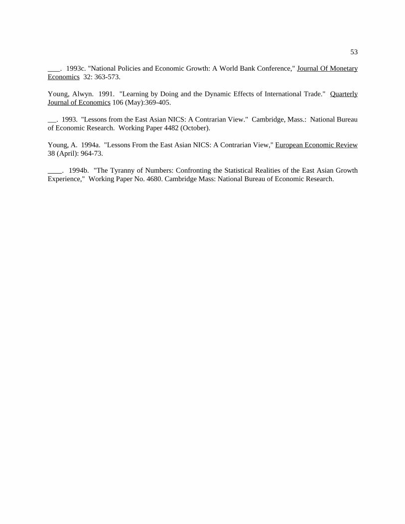
53

. 1993c. "National Policies and Economic Growth: A World Bank Conference," Journal Of MonetaryEconomics 32: 363-573.

Young, Alwyn. 1991. "Learning by Doing and the Dynamic Effects of International Trade." QuarterlyJournal of Economics 106 (May):369-405.

. 1993. "Lessons from the East Asian NICS: A Contrarian View." Cambridge, Mass.: National Bureauof Economic Research. Working Paper 4482 (October).

Young, A. 1994a. "Lessons From the East Asian NICS: A Contrarian View," European Economic Review38 (April): 964-73.

. 1994b. "The Tyranny of Numbers: Confronting the Statistical Realities of the East Asian GrowthExperience," Working Paper No. 4680. Cambridge Mass: National Bureau of Economic Research.

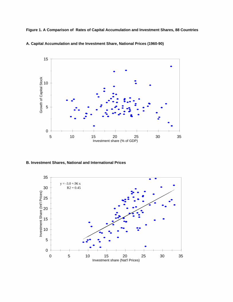
0

5

10

15

20

25

30

35

Inve

stm

ent S

hare

(In

t'l P

rices

)

0 5 10 15 20 25 30 35 Investment share (Nat'l Prices)

y = -3.0 +.96 xR2 = 0.45

0

5

10

15

Gro

wth

of C

apita

l Sto

ck

5 10 15 20 25 30 35 Investment share (% of GDP)

Figure 1. A Comparison of Rates of Capital Accumulation and Investment Shares, 88 Countries

A. Capital Accumulation and the Investment Share, National Prices (1960-90)

B. Investment Shares, National and International Prices

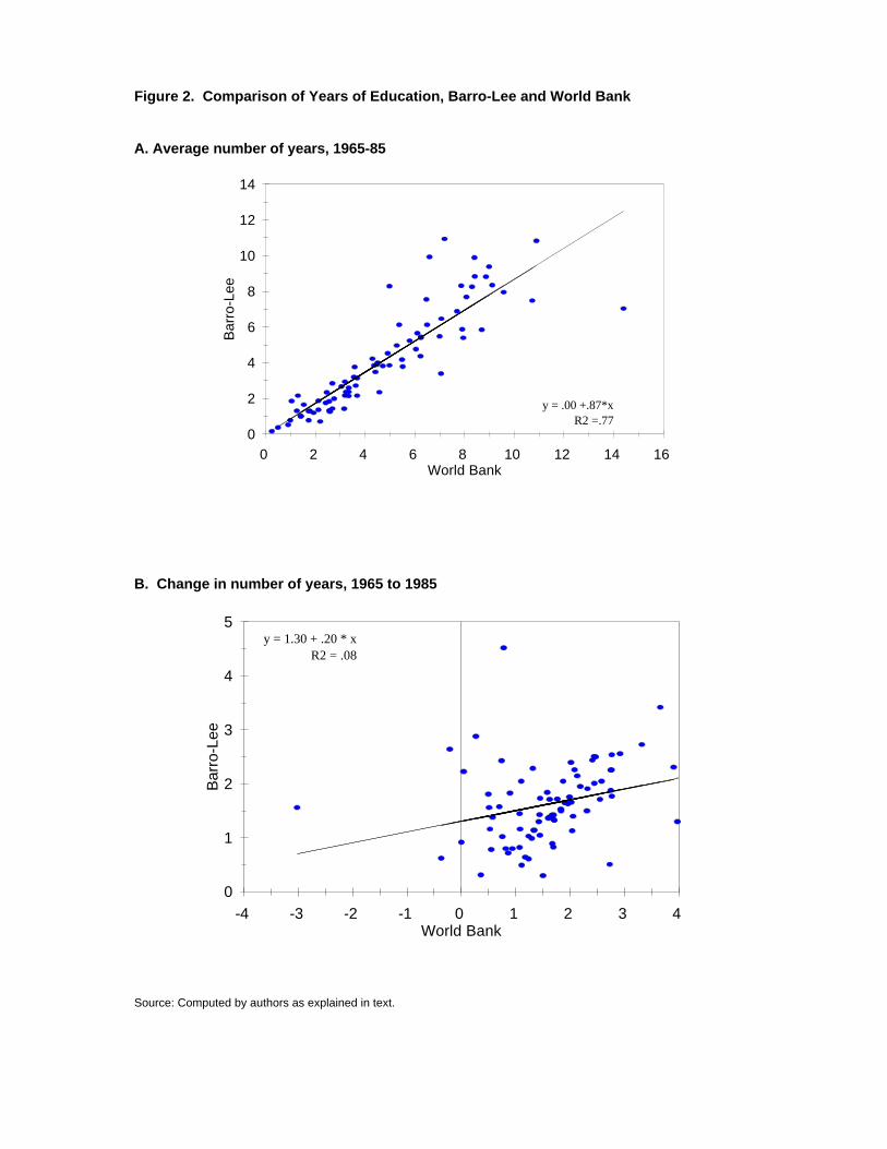
0

1

2

3

4

5

Bar

ro-L

ee

-4 -3 -2 -1 0 1 2 3 4 World Bank

y = 1.30 + .20 * xR2 = .08

0

2

4

6

8

10

12

14

Bar

ro-L

ee

0 2 4 6 8 10 12 14 16 World Bank

y = .00 +.87*xR2 =.77

Figure 2. Comparison of Years of Education, Barro-Lee and World Bank

A. Average number of years, 1965-85

B. Change in number of years, 1965 to 1985

Source: Computed by authors as explained in text.

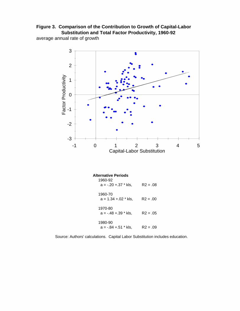
-3

-2

-1

0

1

2

3

Fac

tor

Pro

duct

ivity

-1 0 1 2 3 4 5 Capital-Labor Substitution

Figure 3. Comparison of the Contribution to Growth of Capital-Labor Substitution and Total Factor Productivity, 1960-92 average annual rate of growth

Alternative Periods 1960-92 a = -.20 +.37 * kls, R2 = .08

1960-70 a = 1.34 +.02 * kls, R2 = .00

1970-80 a = -.48 +.39 * kls, R2 = .05

1980-90 a = -.84 +.51 * kls, R2 = .09

Source: Authors' calculations. Capital Labor Substitution includes education.

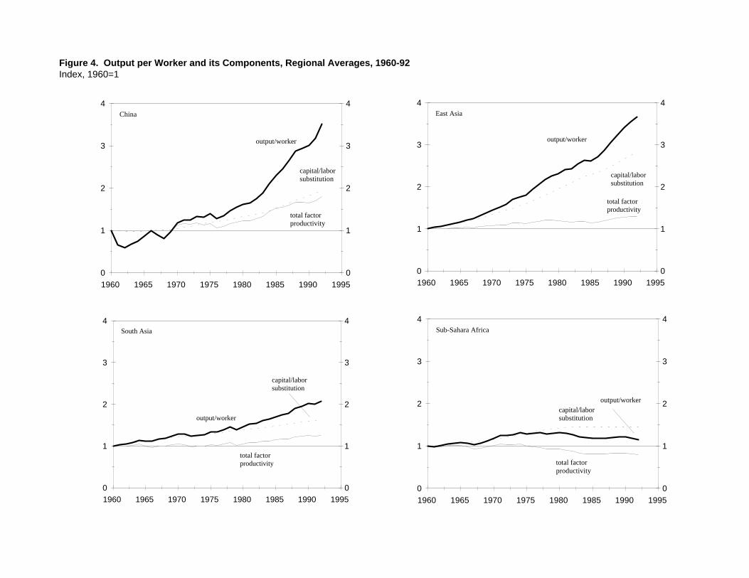
0

1

2

3

4

0

1

2

3

4

1960 1965 1970 1975 1980 1985 1990 1995

output/workercapital/laborsubstitution

total factorproductivity

Sub-Sahara Africa

0

1

2

3

4

0

1

2

3

4

1960 1965 1970 1975 1980 1985 1990 1995

output/worker

capital/laborsubstitution

total factorproductivity

South Asia

0

1

2

3

4

0

1

2

3

4

1960 1965 1970 1975 1980 1985 1990 1995

output/worker

capital/laborsubstitution

total factorproductivity

East Asia

0

1

2

3

4

0

1

2

3

4

1960 1965 1970 1975 1980 1985 1990 1995

output/worker

capital/laborsubstitution

total factorproductivity

China

Figure 4. Output per Worker and its Components, Regional Averages, 1960-92Index, 1960=1

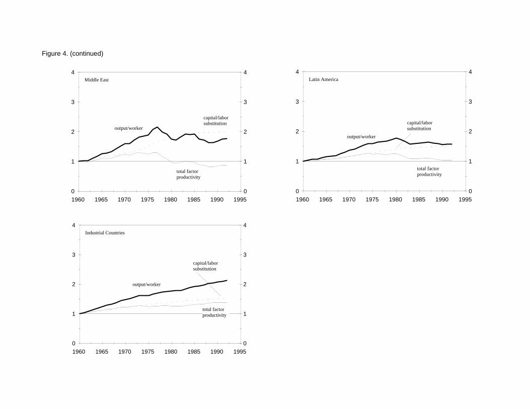
0

1

2

3

4

0

1

2

3

4

1960 1965 1970 1975 1980 1985 1990 1995

output/worker

capital/laborsubstitution

total factorproductivity

Industrial Countries

0

1

2

3

4

0

1

2

3

4

1960 1965 1970 1975 1980 1985 1990 1995

output/worker

capital/laborsubstitution

total factorproductivity

Latin America

0

1

2

3

4

0

1

2

3

4

1960 1965 1970 1975 1980 1985 1990 1995

output/worker

capital/laborsubstitution

total factorproductivity

Middle East

Figure 4. (continued)

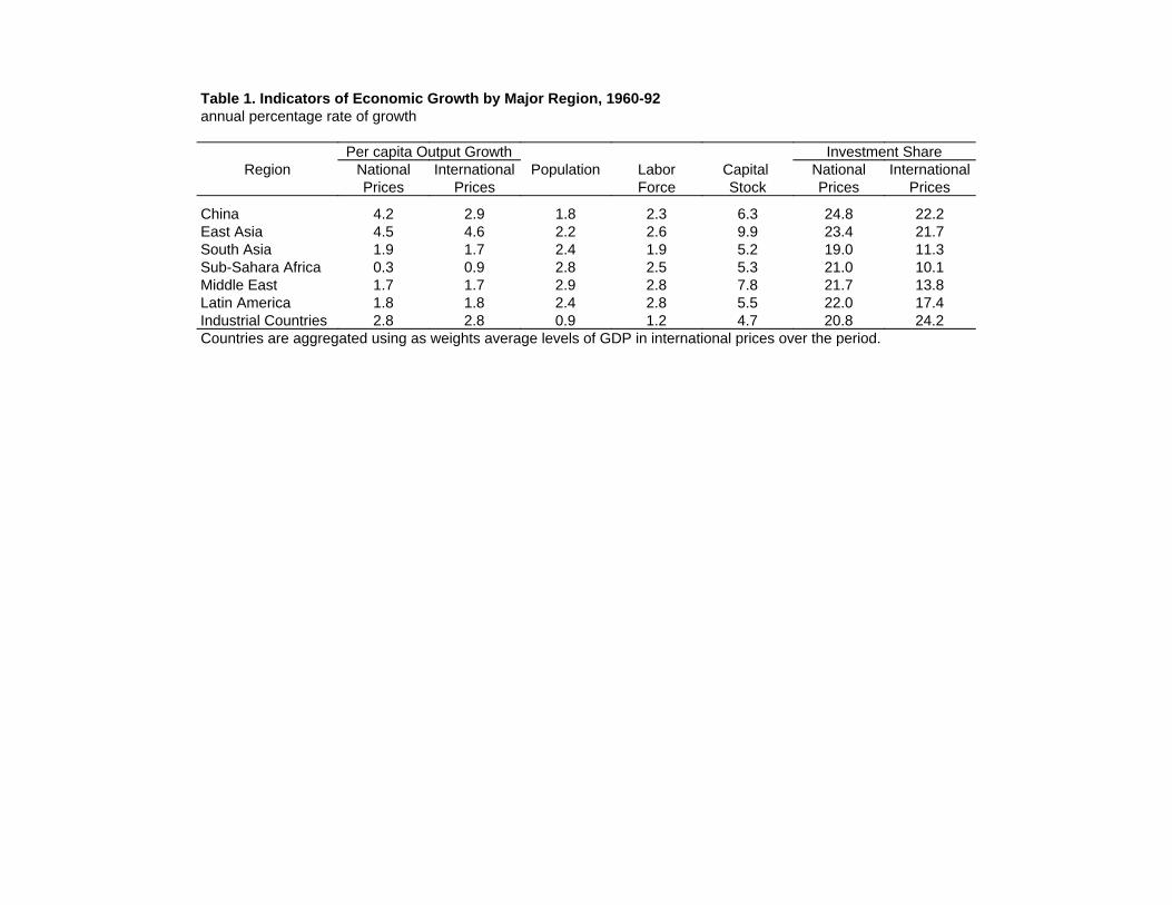
Table 1. Indicators of Economic Growth by Major Region, 1960-92annual percentage rate of growth

Investment SharePer capita Output GrowthInternationalNationalCapital LaborPopulationInternationalNationalRegion

PricesPricesStockForcePricesPrices

22.224.86.32.31.82.94.2China21.723.49.92.62.24.64.5East Asia11.319.05.21.92.41.71.9South Asia10.121.05.32.52.80.90.3Sub-Sahara Africa13.821.77.82.82.91.71.7Middle East17.422.05.52.82.41.81.8Latin America24.220.84.71.20.92.82.8Industrial Countries

Countries are aggregated using as weights average levels of GDP in international prices over the period.

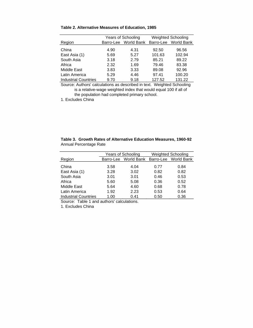
Table 2. Alternative Measures of Education, 1985

Weighted SchoolingYears of SchoolingWorld BankBarro-LeeWorld BankBarro-LeeRegion

96.5692.504.314.90China102.94101.635.275.69East Asia (1)89.2285.212.793.18South Asia83.3879.461.692.32Africa92.9689.083.333.83Middle East100.2097.414.465.29Latin America131.22127.529.189.70Industrial Countries

Source: Authors' calculations as described in text. Weighted Schooling is a relative-wage weighted index that would equal 100 if all of the population had completed primary school.1. Excludes China

Table 3. Growth Rates of Alternative Education Measures, 1960-92Annual Percentage Rate

Weighted SchoolingYears of SchoolingWorld BankBarro-LeeWorld BankBarro-LeeRegion

0.840.774.043.58China0.820.823.023.28East Asia (1)0.530.463.013.01South Asia0.520.365.085.60Africa0.780.684.605.64Middle East0.640.532.231.92Latin America0.360.500.411.00Industrial Countries

Source: Table 1 and authors' calculations.1. Excludes China

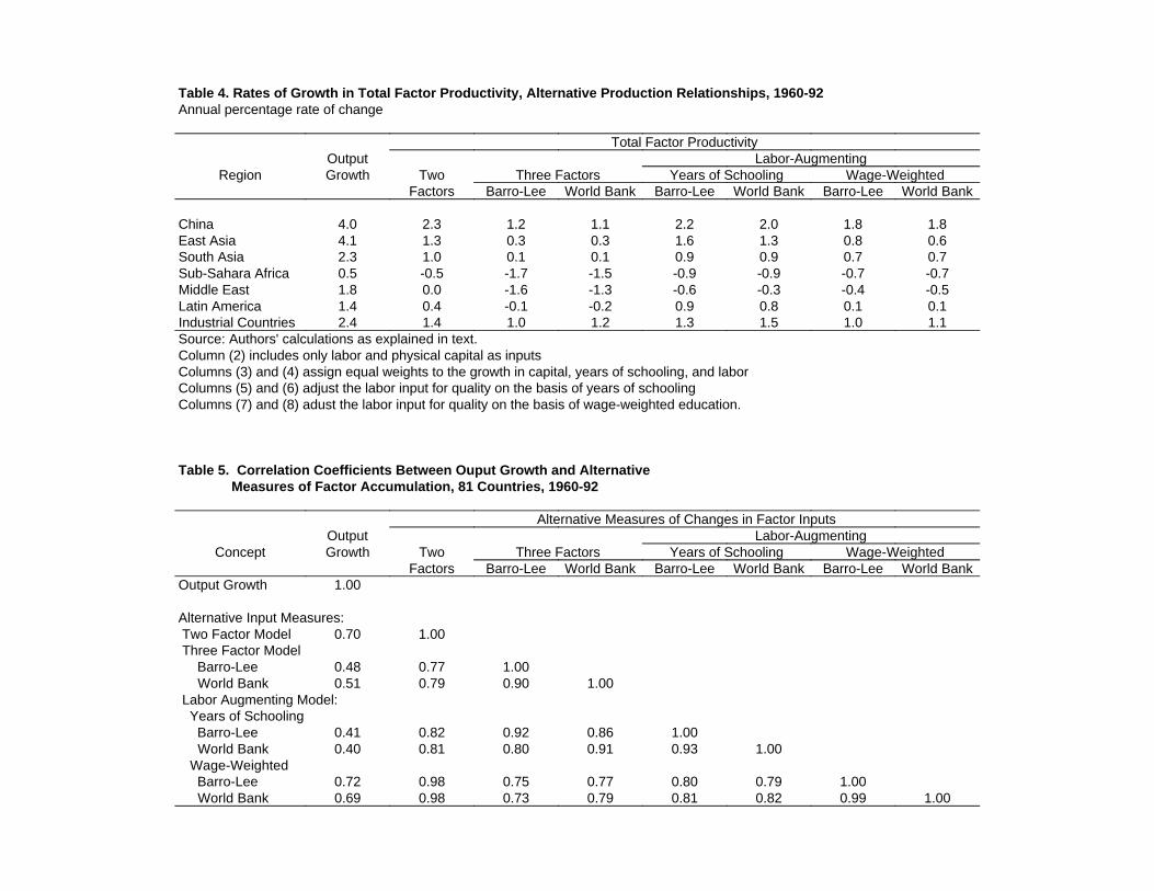
Table 4. Rates of Growth in Total Factor Productivity, Alternative Production Relationships, 1960-92Annual percentage rate of change

Total Factor ProductivityLabor-AugmentingOutput

Wage-WeightedYears of SchoolingThree FactorsTwoGrowthRegionWorld BankBarro-LeeWorld BankBarro-LeeWorld BankBarro-LeeFactors

1.81.82.02.21.11.22.34.0China0.60.81.31.60.30.31.34.1East Asia0.70.70.90.90.10.11.02.3South Asia-0.7-0.7-0.9-0.9-1.5-1.7-0.50.5Sub-Sahara Africa-0.5-0.4-0.3-0.6-1.3-1.60.01.8Middle East0.10.10.80.9-0.2-0.10.41.4Latin America1.11.01.51.31.21.01.42.4Industrial Countries

Source: Authors' calculations as explained in text.Column (2) includes only labor and physical capital as inputsColumns (3) and (4) assign equal weights to the growth in capital, years of schooling, and laborColumns (5) and (6) adjust the labor input for quality on the basis of years of schoolingColumns (7) and (8) adust the labor input for quality on the basis of wage-weighted education.

Table 5. Correlation Coefficients Between Ouput Growth and Alternative Measures of Factor Accumulation, 81 Countries, 1960-92

Alternative Measures of Changes in Factor InputsLabor-AugmentingOutput

Wage-WeightedYears of SchoolingThree FactorsTwoGrowthConceptWorld BankBarro-LeeWorld BankBarro-LeeWorld BankBarro-LeeFactors

1.00Output Growth

Alternative Input Measures:1.000.70 Two Factor Model

Three Factor Model1.000.770.48 Barro-Lee

1.000.900.790.51 World Bank Labor Augmenting Model: Years of Schooling

1.000.860.920.820.41 Barro-Lee1.000.930.910.800.810.40 World Bank

Wage-Weighted1.000.790.800.770.750.980.72 Barro-Lee

1.000.990.820.810.790.730.980.69 World Bank

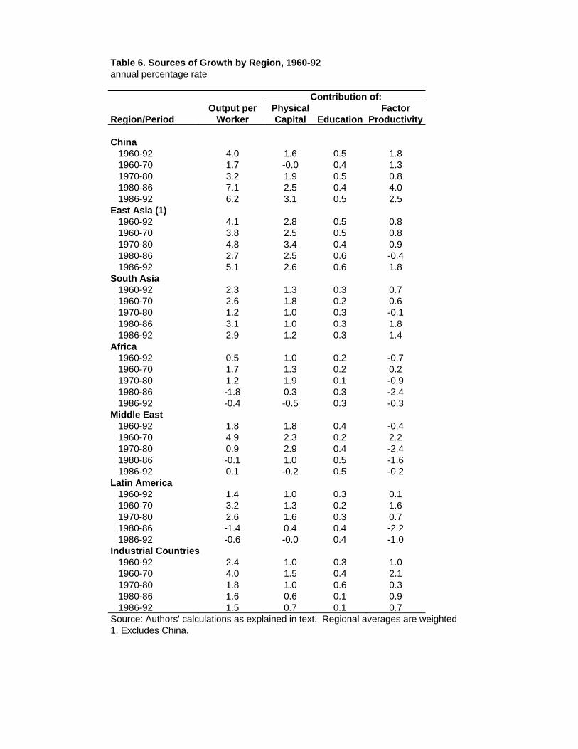
Table 6. Sources of Growth by Region, 1960-92annual percentage rate

Contribution of:FactorPhysicalOutput per

ProductivityEducationCapitalWorkerRegion/Period

China1.80.51.64.0 1960-921.30.4-0.01.7 1960-700.80.51.93.2 1970-804.00.42.57.1 1980-862.50.53.16.2 1986-92

East Asia (1)0.80.52.84.1 1960-920.80.52.53.8 1960-700.90.43.44.8 1970-80-0.40.62.52.7 1980-861.80.62.65.1 1986-92

South Asia0.70.31.32.3 1960-920.60.21.82.6 1960-70-0.10.31.01.2 1970-801.80.31.03.1 1980-861.40.31.22.9 1986-92

Africa-0.70.21.00.5 1960-920.20.21.31.7 1960-70-0.90.11.91.2 1970-80-2.40.30.3-1.8 1980-86-0.30.3-0.5-0.4 1986-92

Middle East-0.40.41.81.8 1960-922.20.22.34.9 1960-70-2.40.42.90.9 1970-80-1.60.51.0-0.1 1980-86-0.20.5-0.20.1 1986-92

Latin America0.10.31.01.4 1960-921.60.21.33.2 1960-700.70.31.62.6 1970-80-2.20.40.4-1.4 1980-86-1.00.4-0.0-0.6 1986-92

Industrial Countries1.00.31.02.4 1960-922.10.41.54.0 1960-700.30.61.01.8 1970-800.90.10.61.6 1980-860.70.10.71.5 1986-92

Source: Authors' calculations as explained in text. Regional averages are weighted1. Excludes China.

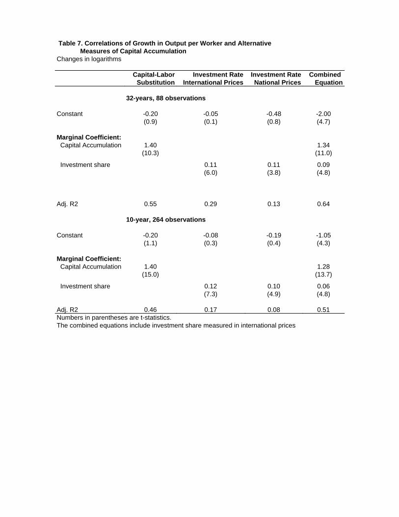
Table 7. Correlations of Growth in Output per Worker and Alternative Measures of Capital AccumulationChanges in logarithms

Combined Investment RateInvestment RateCapital-LaborEquationNational PricesInternational PricesSubstitution

32-years, 88 observations

-2.00-0.48-0.05-0.20Constant(4.7)(0.8)(0.1)(0.9)

Marginal Coefficient:1.341.40 Capital Accumulation

(11.0)(10.3)

0.090.110.11 Investment share(4.8)(3.8)(6.0)

0.640.130.290.55Adj. R2

10-year, 264 observations

-1.05-0.19-0.08-0.20Constant(4.3)(0.4)(0.3)(1.1)

Marginal Coefficient:1.281.40 Capital Accumulation

(13.7)(15.0)

0.060.100.12 Investment share(4.8)(4.9)(7.3)

0.510.080.170.46Adj. R2Numbers in parentheses are t-statistics.The combined equations include investment share measured in international prices

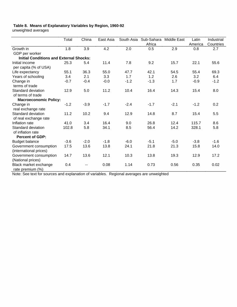
Table 8. Means of Explanatory Variables by Region, 1960-92unweighted averages

IndustrialLatinMiddle EastSub-SaharaSouth AsiaEast AsiaChinaTotalCountriesAmericaAfrica

2.70.82.90.52.04.23.91.8Growth in GDP per worker Initial Conditions and External Shocks:

55.622.115.79.27.811.45.425.3Initial income per capita (% of USA)

69.355.454.542.147.755.036.355.1Life expectancy6.43.22.61.21.73.32.13.4Years of schooling-1.2-0.91.7-1.3-1.2-0.0-0.4-0.7Change in

terms of trade8.015.414.316.410.411.25.012.9Standard deviation

of terms of trade Macroeconomic Policy:

0.2-1.2-2.1-1.7-2.4-1.7-3.9-1.2Change in real exchange rate

5.515.48.714.812.99.410.211.2Standard deviation of real exchange rate

8.6115.712.426.89.016.43.441.0Inflation rate5.8328.114.256.48.534.15.8102.8Standard deviation

of inflation rate Percent of GDP:

-1.6-3.8-5.0-5.1-6.0-1.8-2.0-3.6Budget balance14.015.821.321.824.113.813.617.5Government consumption

(international prices)17.212.919.313.810.312.113.614.7Government consumption

(National prices)0.020.350.560.731.140.08--0.4Black market exchange

rate premium (%)Note: See text for sources and explanation of variables. Regional averages are unweighted

Table 9. Regression Results for Changes in Output per Worker and its Components, Initial conditions, 32 year sampleChanges in logarithms

TFPCapital per WorkerOutput per workerVariable(7)(6)(5)(4)(3)(2)(1)

-0.4-0.3-0.04-0.04-0.03-0.05-0.06Initial income(3.8)(3.4)(2.5)(2.5)(2.9)(4.5)(4.9)

0.170.19-0.150.140.190.090.26Years of(1.9)(2.0)(0.9)(0.7)(1.9)(0.8)(1.9)schooling

0.030.040.060.070.040.060.07Life expectancy(1.9)(2.4)(2.0)(2.1)(2.2)(2.9)(3.0)

0.060.140.080.370.130.090.3Change in tot(1.1)(2.7)(0.7)(3.4)(2.3)(1.2)(4.3)

-0.03-0.07-0.03-0.13-0.07-0.05-0.12Standard Dev.(1.9)(3.8)(0.8)(3.4)(3.3)(2.0)(4.9)of tot

1.08Capital-labor(8.2)substitution

yesnoyesnonoyesnoRegionaldummies

0.5-4.0-1.7 South Asia(0.1)(4.3)(3.0)

-0.4-4.5-2.6 Africa(1.0)(5.6)(5.0)

0.3-2.9-1.0 Middle East(0.8)(3.8)(2.0)

-0.7-4.4-2.7 Latin America(1.7)(6.0)(5.8)

0.8-1.6-0.5 Industrial cntry.(1.7)(1.7)(0.8)

0.490.390.500.220.700.650.45Adj. R2Numbers in parentheses are t-statistics. Changes in logarithms are multiplied by 100.

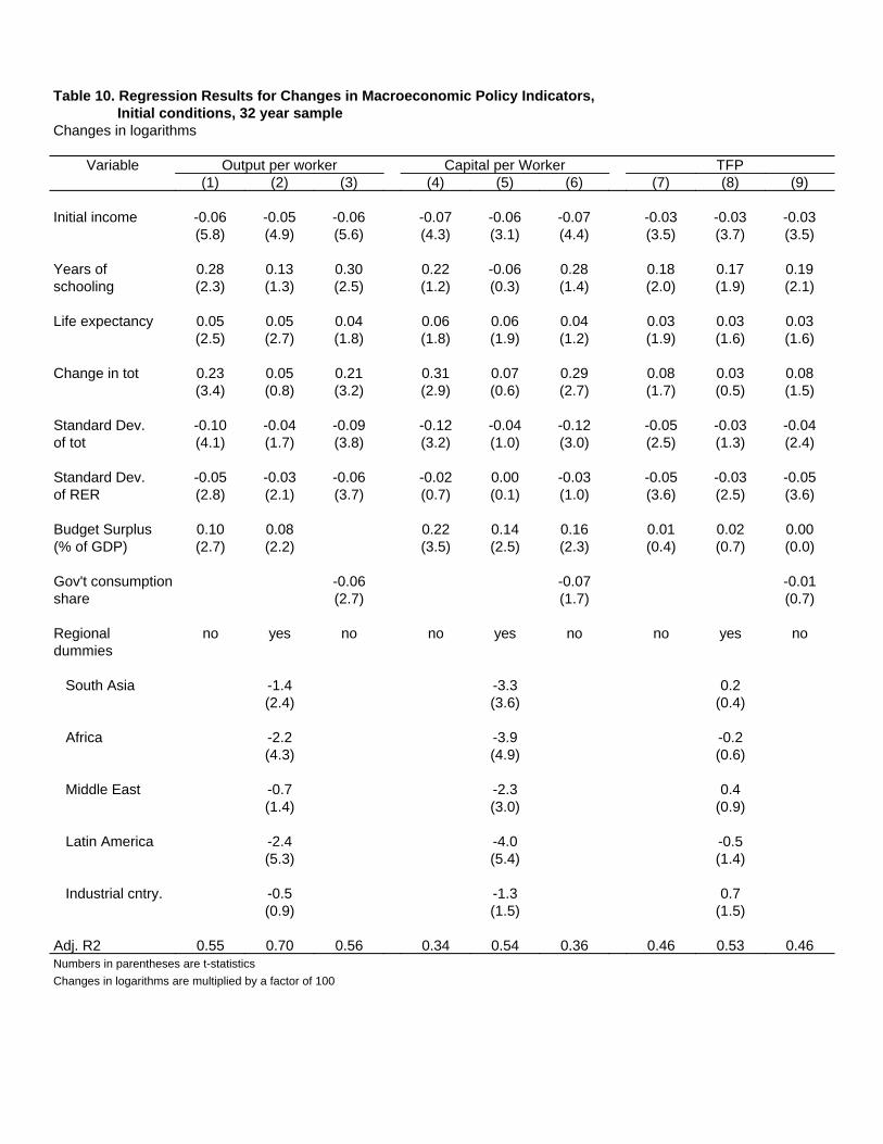
Table 10. Regression Results for Changes in Macroeconomic Policy Indicators, Initial conditions, 32 year sampleChanges in logarithms

TFPCapital per WorkerOutput per workerVariable(9)(8)(7)(6)(5)(4)(3)(2)(1)

-0.03-0.03-0.03-0.07-0.06-0.07-0.06-0.05-0.06Initial income(3.5)(3.7)(3.5)(4.4)(3.1)(4.3)(5.6)(4.9)(5.8)

0.190.170.180.28-0.060.220.300.130.28Years of(2.1)(1.9)(2.0)(1.4)(0.3)(1.2)(2.5)(1.3)(2.3)schooling

0.030.030.030.040.060.060.040.050.05Life expectancy(1.6)(1.6)(1.9)(1.2)(1.9)(1.8)(1.8)(2.7)(2.5)

0.080.030.080.290.070.310.210.050.23Change in tot(1.5)(0.5)(1.7)(2.7)(0.6)(2.9)(3.2)(0.8)(3.4)

-0.04-0.03-0.05-0.12-0.04-0.12-0.09-0.04-0.10Standard Dev.(2.4)(1.3)(2.5)(3.0)(1.0)(3.2)(3.8)(1.7)(4.1)of tot

-0.05-0.03-0.05-0.030.00-0.02-0.06-0.03-0.05Standard Dev.(3.6)(2.5)(3.6)(1.0)(0.1)(0.7)(3.7)(2.1)(2.8)of RER

0.000.020.010.160.140.220.080.10Budget Surplus(0.0)(0.7)(0.4)(2.3)(2.5)(3.5)(2.2)(2.7)(% of GDP)

-0.01-0.07-0.06Gov't consumption(0.7)(1.7)(2.7)share

noyesnonoyesnonoyesnoRegionaldummies

0.2-3.3-1.4 South Asia(0.4)(3.6)(2.4)

-0.2-3.9-2.2 Africa(0.6)(4.9)(4.3)

0.4-2.3-0.7 Middle East(0.9)(3.0)(1.4)

-0.5-4.0-2.4 Latin America(1.4)(5.4)(5.3)

0.7-1.3-0.5 Industrial cntry.(1.5)(1.5)(0.9)

0.460.530.460.360.540.340.560.700.55Adj. R2Numbers in parentheses are t-statistics

Changes in logarithms are multiplied by a factor of 100

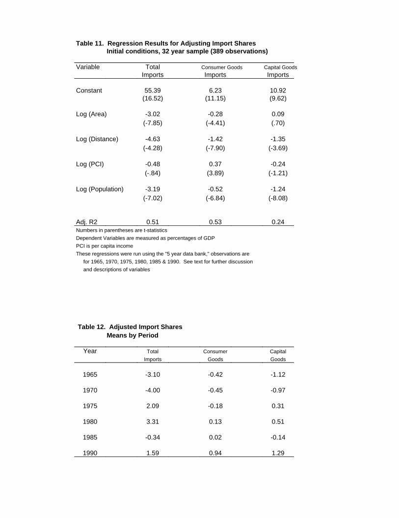
Table 11. Regression Results for Adjusting Import Shares Initial conditions, 32 year sample (389 observations)

Capital GoodsConsumer GoodsTotalVariableImportsImportsImports

10.926.2355.39Constant(9.62)(11.15)(16.52)

0.09-0.28-3.02Log (Area)(.70)(-4.41)(-7.85)

-1.35-1.42-4.63Log (Distance)(-3.69)(-7.90)(-4.28)

-0.240.37-0.48Log (PCI)(-1.21)(3.89)(-.84)

-1.24-0.52-3.19Log (Population)(-8.08)(-6.84)(-7.02)

0.240.530.51Adj. R2Numbers in parentheses are t-statistics

Dependent Variables are measured as percentages of GDP

PCI is per capita income

These regressions were run using the "5 year data bank," observations are

for 1965, 1970, 1975, 1980, 1985 & 1990. See text for further discussion

and descriptions of variables

Table 12. Adjusted Import Shares Means by Period

CapitalConsumerTotalYearGoodsGoodsImports

-1.12-0.42-3.101965

-0.97-0.45-4.001970

0.31-0.182.091975

0.510.133.311980

-0.140.02-0.341985

1.290.941.591990

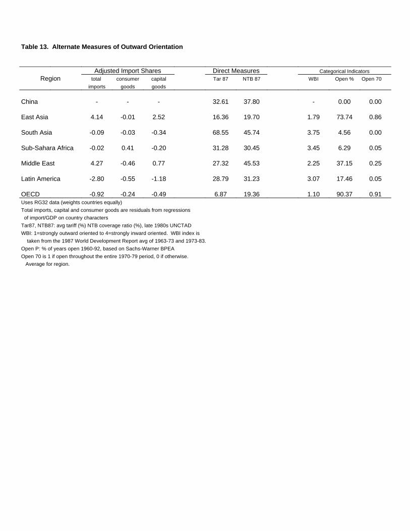
Table 13. Alternate Measures of Outward Orientation

Categorical IndicatorsDirect MeasuresAdjusted Import SharesOpen 70Open %WBINTB 87Tar 87capitalconsumertotal Region

goodsgoodsimports

0.000.00-37.8032.61---China

0.8673.741.7919.7016.362.52-0.014.14East Asia

0.004.563.7545.7468.55-0.34-0.03-0.09South Asia

0.056.293.4530.4531.28-0.200.41-0.02Sub-Sahara Africa

0.2537.152.2545.5327.320.77-0.464.27Middle East

0.0517.463.0731.2328.79-1.18-0.55-2.80Latin America

0.9190.371.1019.366.87-0.49-0.24-0.92OECDUses RG32 data (weights countries equally)

Total imports, capital and consumer goods are residuals from regressions

of import/GDP on country characters

Tar87, NTB87: avg tariff (%) NTB coverage ratio (%), late 1980s UNCTAD

WBI: 1=strongly outward oriented to 4=strongly inward oriented. WBI index is

taken from the 1987 World Development Report avg of 1963-73 and 1973-83.

Open P: % of years open 1960-92, based on Sachs-Warner BPEA

Open 70 is 1 if open throughout the entire 1970-79 period, 0 if otherwise.

Average for region.

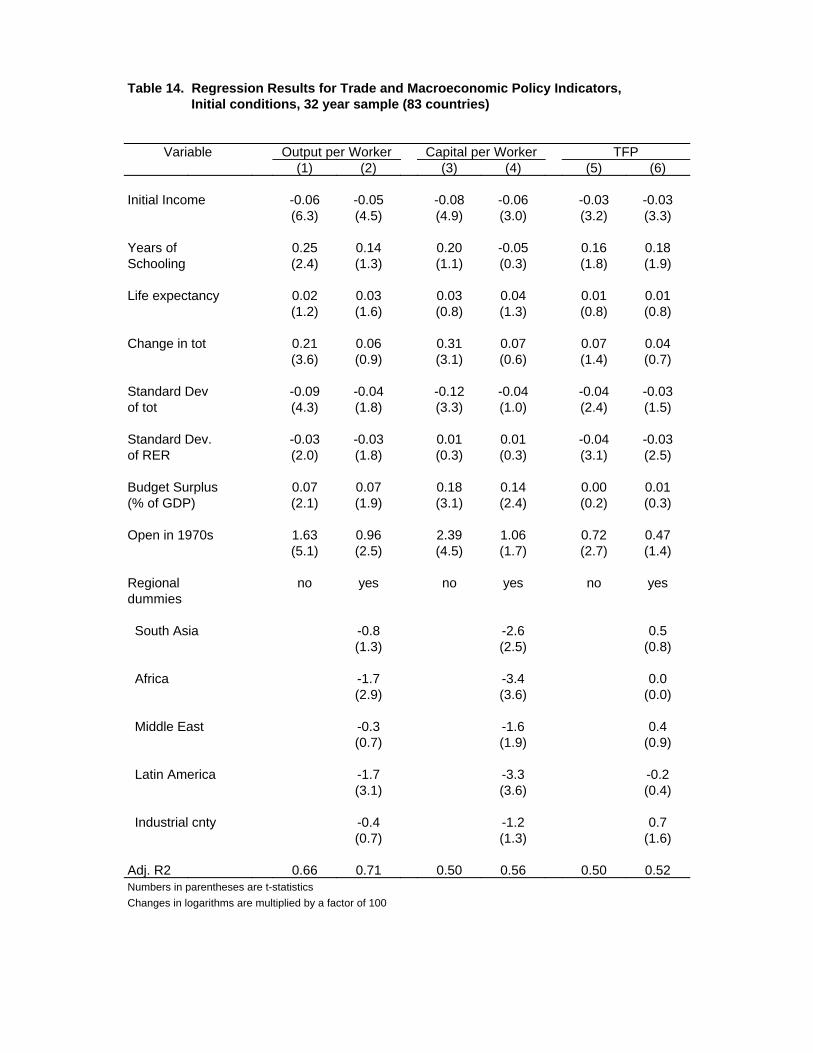
Table 14. Regression Results for Trade and Macroeconomic Policy Indicators,Initial conditions, 32 year sample (83 countries)

TFPCapital per WorkerOutput per WorkerVariable(6)(5)(4)(3)(2)(1)

-0.03-0.03-0.06-0.08-0.05-0.06Initial Income(3.3)(3.2)(3.0)(4.9)(4.5)(6.3)

0.180.16-0.050.200.140.25Years of(1.9)(1.8)(0.3)(1.1)(1.3)(2.4)Schooling

0.010.010.040.030.030.02Life expectancy(0.8)(0.8)(1.3)(0.8)(1.6)(1.2)

0.040.070.070.310.060.21Change in tot(0.7)(1.4)(0.6)(3.1)(0.9)(3.6)

-0.03-0.04-0.04-0.12-0.04-0.09Standard Dev(1.5)(2.4)(1.0)(3.3)(1.8)(4.3)of tot

-0.03-0.040.010.01-0.03-0.03Standard Dev.(2.5)(3.1)(0.3)(0.3)(1.8)(2.0)of RER

0.010.000.140.180.070.07Budget Surplus(0.3)(0.2)(2.4)(3.1)(1.9)(2.1)(% of GDP)

0.470.721.062.390.961.63Open in 1970s(1.4)(2.7)(1.7)(4.5)(2.5)(5.1)

yesnoyesnoyesnoRegionaldummies

0.5-2.6-0.8 South Asia(0.8)(2.5)(1.3)

0.0-3.4-1.7 Africa(0.0)(3.6)(2.9)

0.4-1.6-0.3 Middle East(0.9)(1.9)(0.7)

-0.2-3.3-1.7 Latin America(0.4)(3.6)(3.1)

0.7-1.2-0.4 Industrial cnty(1.6)(1.3)(0.7)

0.520.500.560.500.710.66Adj. R2Numbers in parentheses are t-statistics

Changes in logarithms are multiplied by a factor of 100

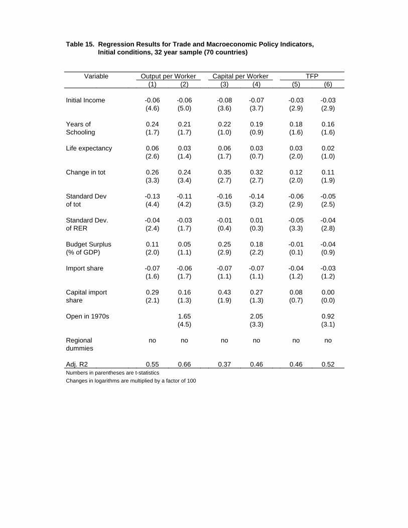
Table 15. Regression Results for Trade and Macroeconomic Policy Indicators,Initial conditions, 32 year sample (70 countries)

TFPCapital per WorkerOutput per WorkerVariable(6)(5)(4)(3)(2)(1)

-0.03-0.03-0.07-0.08-0.06-0.06Initial Income(2.9)(2.9)(3.7)(3.6)(5.0)(4.6)

0.160.180.190.220.210.24Years of(1.6)(1.6)(0.9)(1.0)(1.7)(1.7)Schooling

0.020.030.030.060.030.06Life expectancy(1.0)(2.0)(0.7)(1.7)(1.4)(2.6)

0.110.120.320.350.240.26Change in tot(1.9)(2.0)(2.7)(2.7)(3.4)(3.3)

-0.05-0.06-0.14-0.16-0.11-0.13Standard Dev(2.5)(2.9)(3.2)(3.5)(4.2)(4.4)of tot

-0.04-0.050.01-0.01-0.03-0.04Standard Dev.(2.8)(3.3)(0.3)(0.4)(1.7)(2.4)of RER

-0.04-0.010.180.250.050.11Budget Surplus(0.9)(0.1)(2.2)(2.9)(1.1)(2.0)(% of GDP)

-0.03-0.04-0.07-0.07-0.06-0.07Import share(1.2)(1.2)(1.1)(1.1)(1.7)(1.6)

0.000.080.270.430.160.29Capital import (0.0)(0.7)(1.3)(1.9)(1.3)(2.1)share

0.922.051.65Open in 1970s(3.1)(3.3)(4.5)

nonononononoRegionaldummies

0.520.460.460.370.660.55Adj. R2Numbers in parentheses are t-statistics

Changes in logarithms are multiplied by a factor of 100

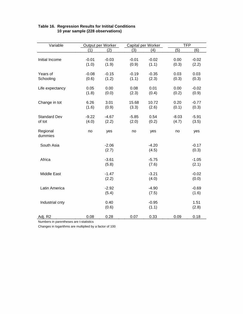
Table 16. Regression Results for Initital Conditions10 year sample (228 observations)

TFPCapital per WorkerOutput per WorkerVariable(6)(5)(4)(3)(2)(1)

-0.020.00-0.02-0.01-0.03-0.01Initial Income(2.2)(0.3)(1.1)(0.9)(1.9)(1.0)

0.030.03-0.35-0.19-0.15-0.08Years of(0.3)(0.3)(2.3)(1.1)(1.2)(0.6)Schooling

-0.020.000.010.080.000.05Life expectancy(0.9)(0.2)(0.4)(2.3)(0.0)(1.8)

-0.770.2010.7215.683.016.26Change in tot(0.3)(0.1)(2.6)(3.3)(0.9)(1.6)

-5.91-8.030.54-5.85-4.67-9.22Standard Dev(3.5)(4.7)(0.2)(2.0)(2.2)(4.0)of tot

yesnoyesnoyesnoRegionaldummies

-0.17-4.20-2.06 South Asia(0.3)(4.5)(2.7)

-1.05-5.75-3.61 Africa(2.1)(7.6)(5.8)

-0.02-3.21-1.47 Middle East(0.0)(4.0)(2.2)

-0.69-4.90-2.92 Latin America(1.6)(7.5)(5.4)

1.51-0.950.40 Industrial cnty(2.8)(1.1)(0.6)

0.180.090.330.070.280.08Adj. R2Numbers in parentheses are t-statistics

Changes in logarithms are multiplied by a factor of 100

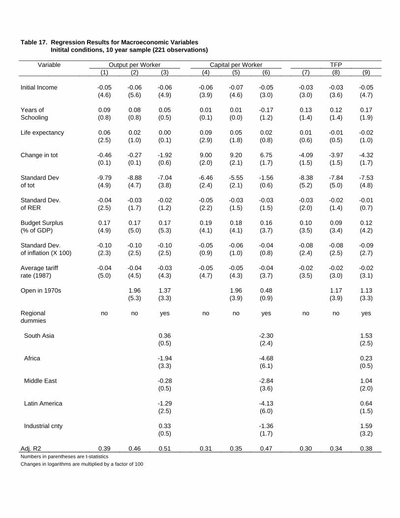
Table 17. Regression Results for Macroeconomic VariablesInitital conditions, 10 year sample (221 observations)

TFPCapital per WorkerOutput per WorkerVariable(9)(8)(7)(6)(5)(4)(3)(2)(1)

-0.05-0.03-0.03-0.05-0.07-0.06-0.06-0.06-0.05Initial Income(4.7)(3.6)(3.0)(3.0)(4.6)(3.9)(4.9)(5.6)(4.6)

0.170.120.13-0.170.010.010.050.080.09Years of(1.9)(1.4)(1.4)(1.2)(0.0)(0.1)(0.5)(0.8)(0.8)Schooling

-0.02-0.010.010.020.050.090.000.020.06Life expectancy(1.0)(0.5)(0.6)(0.8)(1.8)(2.9)(0.1)(1.0)(2.5)

-4.32-3.97-4.096.759.209.00-1.92-0.27-0.46Change in tot(1.7)(1.5)(1.5)(1.7)(2.1)(2.0)(0.6)(0.1)(0.1)

-7.53-7.84-8.38-1.56-5.55-6.46-7.04-8.88-9.79Standard Dev(4.8)(5.0)(5.2)(0.6)(2.1)(2.4)(3.8)(4.7)(4.9)of tot

-0.01-0.02-0.03-0.03-0.03-0.05-0.02-0.03-0.04Standard Dev.(0.7)(1.4)(2.0)(1.5)(1.5)(2.2)(1.2)(1.7)(2.5)of RER

0.120.090.100.160.180.190.170.170.17Budget Surplus(4.2)(3.4)(3.5)(3.7)(4.1)(4.1)(5.3)(5.0)(4.9)(% of GDP)

-0.09-0.08-0.08-0.04-0.06-0.05-0.10-0.10-0.10Standard Dev.(2.7)(2.5)(2.4)(0.8)(1.0)(0.9)(2.5)(2.5)(2.3)of inflation (X 100)

-0.02-0.02-0.02-0.04-0.05-0.05-0.03-0.04-0.04Average tariff(3.1)(3.0)(3.5)(3.7)(4.3)(4.7)(4.3)(4.5)(5.0)rate (1987)

1.131.170.481.961.371.96Open in 1970s(3.3)(3.9)(0.9)(3.9)(3.3)(5.3)

yesnonoyesnonoyesnonoRegionaldummies

1.53-2.300.36 South Asia(2.5)(2.4)(0.5)

0.23-4.68-1.94 Africa(0.5)(6.1)(3.3)

1.04-2.84-0.28 Middle East(2.0)(3.6)(0.5)

0.64-4.13-1.29 Latin America(1.5)(6.0)(2.5)

1.59-1.360.33 Industrial cnty(3.2)(1.7)(0.5)

0.380.340.300.470.350.310.510.460.39Adj. R2Numbers in parentheses are t-statistics

Changes in logarithms are multiplied by a factor of 100

Appendix Table 1. List of Included Countries, by Region

Middle East and Industrial countriesNorth AfricaEast AsiaAustraliaChinaAustriaAlgeriaIndonesiaBelgiumCyprusKoreaCanadaEgyptMalaysiaDenmarkIranPhilippinesFinlandIsraelSinaporeFranceJordonTaiwan GermanyMaltaThailandGreeceMoroccoIcelandTunisiaSouth AsiaIrelandBangladeshItalyLatin AmericaIndiaJapanArgentinaMyanmarNetherlandsBoliviaPakistanNew ZealandBrazilSri LankaNorwayChilePortugalColumbiaSub-Sahara AfricaSpainCosta RicaCameroonSwedenDominican Rep.Cote d' IvoireSwitzerlandEcuadorEthiopiaTurkeyEl SalvadoreGhanaUnited KingdomGuatemalaKenyaUnited StatesGuyanaMadagascar

HaitiMalawiHondurasMaliJamaicaMauritiusMexicoMozambiqueNicaraguaNigeriaPanamaRwandaParaguaySenegalPeruSierra LeoneTrinidad & TobagoSouth AfricaUruguaySudanVenezuelaTanzania

UgandaZaireZambiaZimbabwe

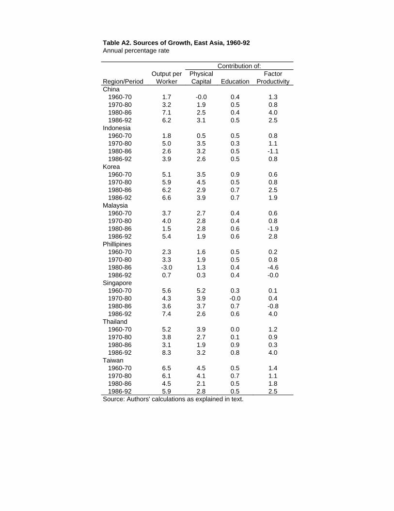
Table A2. Sources of Growth, East Asia, 1960-92Annual percentage rate

Contribution of:FactorPhysicalOutput per

ProductivityEducationCapitalWorkerRegion/PeriodChina

1.30.4-0.01.7 1960-700.80.51.93.2 1970-804.00.42.57.1 1980-862.50.53.16.2 1986-92

Indonesia0.80.50.51.8 1960-701.10.33.55.0 1970-80-1.10.53.22.6 1980-860.80.52.63.9 1986-92

Korea0.60.93.55.1 1960-700.80.54.55.9 1970-802.50.72.96.2 1980-861.90.73.96.6 1986-92

Malaysia0.60.42.73.7 1960-700.80.42.84.0 1970-80-1.90.62.81.5 1980-862.80.61.95.4 1986-92

Phillipines0.20.51.62.3 1960-700.80.51.93.3 1970-80-4.60.41.3-3.0 1980-86-0.00.40.30.7 1986-92

Singapore0.10.35.25.6 1960-700.4-0.03.94.3 1970-80-0.80.73.73.6 1980-864.00.62.67.4 1986-92

Thailand1.20.03.95.2 1960-700.90.12.73.8 1970-800.30.91.93.1 1980-864.00.83.28.3 1986-92

Taiwan1.40.54.56.5 1960-701.10.74.16.1 1970-801.80.52.14.5 1980-862.50.52.85.9 1986-92

Source: Authors' calculations as explained in text.

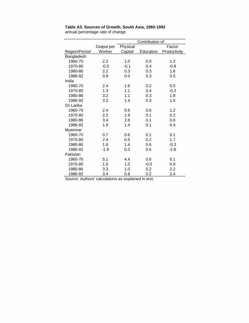
Table A3. Sources of Growth, South Asia, 1960-1992annual percentage rate of change

Contribution of:FactorPhysicalOutput per

ProductivityEducationCapitalWorkerRegion/PeriodBangladesh

1.20.01.02.2 1960-70-0.80.4-0.1-0.5 1970-801.60.30.32.2 1980-860.50.30.00.9 1986-92

India0.50.21.62.4 1960-70-0.20.41.11.3 1970-801.80.31.13.2 1980-861.50.31.43.3 1986-92

Sri Lanka1.20.60.62.4 1960-700.20.11.92.2 1970-800.60.12.63.4 1980-860.40.11.41.9 1986-92

Myanmar0.10.10.60.7 1960-701.70.20.52.4 1970-80-0.30.61.41.8 1980-86-2.80.60.3-1.9 1986-92

Pakistan0.10.64.45.1 1960-700.9-0.01.01.9 1970-802.20.21.03.3 1980-862.40.20.83.4 1986-92

Source: Authors' calculations as explained in text.

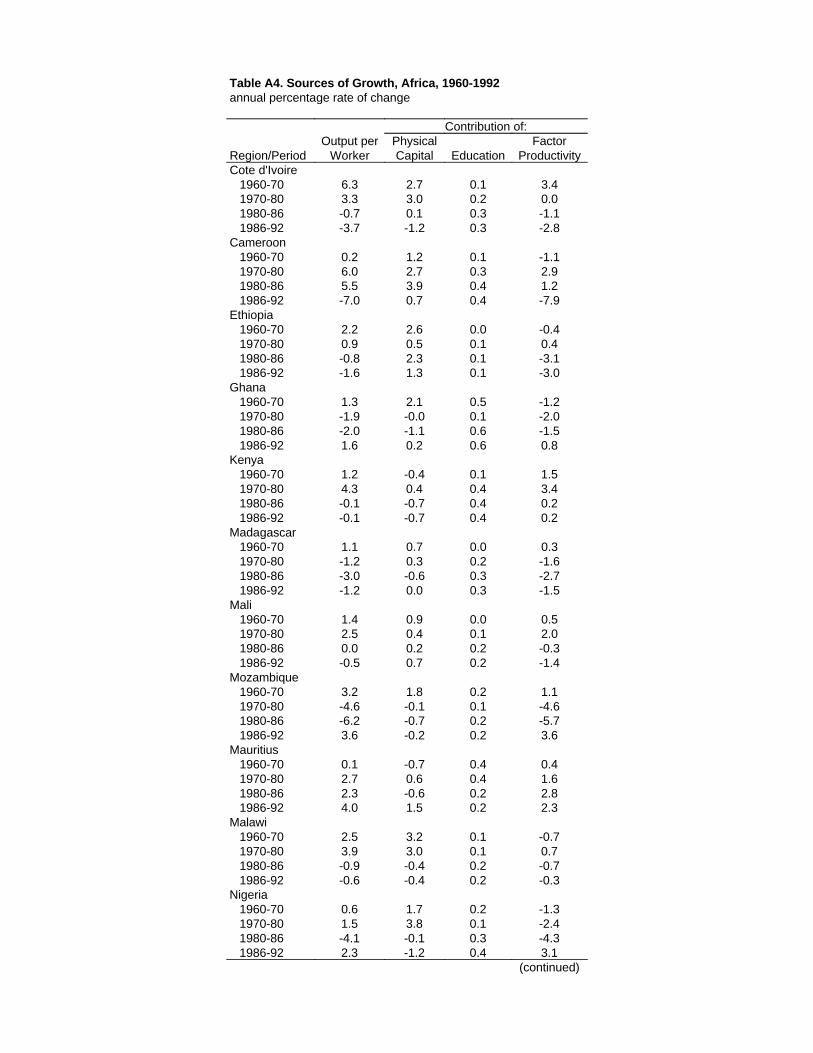
Table A4. Sources of Growth, Africa, 1960-1992annual percentage rate of change

Contribution of:FactorPhysicalOutput per

ProductivityEducationCapitalWorkerRegion/PeriodCote d'Ivoire

3.40.12.76.3 1960-700.00.23.03.3 1970-80-1.10.30.1-0.7 1980-86-2.80.3-1.2-3.7 1986-92

Cameroon-1.10.11.20.2 1960-702.90.32.76.0 1970-801.20.43.95.5 1980-86-7.90.40.7-7.0 1986-92

Ethiopia-0.40.02.62.2 1960-700.40.10.50.9 1970-80-3.10.12.3-0.8 1980-86-3.00.11.3-1.6 1986-92

Ghana-1.20.52.11.3 1960-70-2.00.1-0.0-1.9 1970-80-1.50.6-1.1-2.0 1980-860.80.60.21.6 1986-92

Kenya1.50.1-0.41.2 1960-703.40.40.44.3 1970-800.20.4-0.7-0.1 1980-860.20.4-0.7-0.1 1986-92

Madagascar0.30.00.71.1 1960-70-1.60.20.3-1.2 1970-80-2.70.3-0.6-3.0 1980-86-1.50.30.0-1.2 1986-92

Mali0.50.00.91.4 1960-702.00.10.42.5 1970-80-0.30.20.20.0 1980-86-1.40.20.7-0.5 1986-92

Mozambique1.10.21.83.2 1960-70-4.60.1-0.1-4.6 1970-80-5.70.2-0.7-6.2 1980-863.60.2-0.23.6 1986-92

Mauritius0.40.4-0.70.1 1960-701.60.40.62.7 1970-802.80.2-0.62.3 1980-862.30.21.54.0 1986-92

Malawi-0.70.13.22.5 1960-700.70.13.03.9 1970-80-0.70.2-0.4-0.9 1980-86-0.30.2-0.4-0.6 1986-92

Nigeria-1.30.21.70.6 1960-70-2.40.13.81.5 1970-80-4.30.3-0.1-4.1 1980-863.10.4-1.22.3 1986-92

(continued)

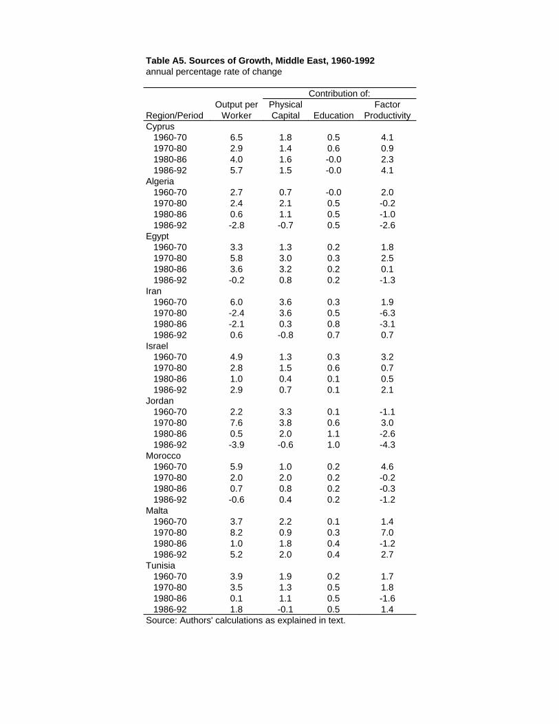
Table A5. Sources of Growth, Middle East, 1960-1992annual percentage rate of change

Contribution of:FactorPhysicalOutput per

ProductivityEducationCapitalWorkerRegion/PeriodCyprus

4.10.51.86.5 1960-700.90.61.42.9 1970-802.3-0.01.64.0 1980-864.1-0.01.55.7 1986-92

Algeria2.0-0.00.72.7 1960-70-0.20.52.12.4 1970-80-1.00.51.10.6 1980-86-2.60.5-0.7-2.8 1986-92

Egypt1.80.21.33.3 1960-702.50.33.05.8 1970-800.10.23.23.6 1980-86-1.30.20.8-0.2 1986-92

Iran1.90.33.66.0 1960-70-6.30.53.6-2.4 1970-80-3.10.80.3-2.1 1980-860.70.7-0.80.6 1986-92

Israel3.20.31.34.9 1960-700.70.61.52.8 1970-800.50.10.41.0 1980-862.10.10.72.9 1986-92

Jordan-1.10.13.32.2 1960-703.00.63.87.6 1970-80-2.61.12.00.5 1980-86-4.31.0-0.6-3.9 1986-92

Morocco4.60.21.05.9 1960-70-0.20.22.02.0 1970-80-0.30.20.80.7 1980-86-1.20.20.4-0.6 1986-92

Malta1.40.12.23.7 1960-707.00.30.98.2 1970-80-1.20.41.81.0 1980-862.70.42.05.2 1986-92

Tunisia1.70.21.93.9 1960-701.80.51.33.5 1970-80-1.60.51.10.1 1980-861.40.5-0.11.8 1986-92

Source: Authors' calculations as explained in text.

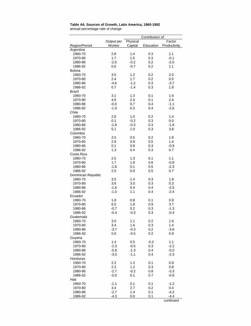
Table A6. Sources of Growth, Latin America, 1960-1992annual percentage rate of change

Contribution of:FactorPhysicalOutput per

ProductivityEducationCapitalWorkerRegion/PeriodArgentina

1.10.31.42.8 1960-70-0.10.31.51.7 1970-80-2.00.2-0.2-2.0 1980-861.10.2-0.70.6 1986-92

Bolivia2.00.21.23.5 1960-700.50.21.72.4 1970-80-3.70.3-1.2-4.6 1980-861.80.3-1.40.7 1986-92

Brazil1.60.11.33.1 1960-702.40.12.44.9 1970-80-1.10.40.7-0.0 1980-86-2.60.40.3-1.9 1986-92

Chile1.40.21.02.6 1960-700.00.3-0.20.1 1970-80-1.90.3-0.3-1.9 1980-863.80.31.05.1 1986-92

Colombia1.80.20.52.5 1960-701.40.50.92.9 1970-80-0.90.30.80.1 1980-860.70.30.41.3 1986-92

Costa Rica1.10.11.32.5 1960-70-0.80.61.81.7 1970-80-2.30.50.1-1.8 1980-860.70.50.92.0 1986-92

Dominican Republic1.80.31.43.5 1960-700.30.33.03.6 1970-80-2.50.40.4-1.6 1980-86-2.40.41.1-1.0 1986-92

Ecuador0.80.10.81.8 1960-703.70.91.86.5 1970-80-1.30.30.2-0.7 1980-86-0.40.3-0.3-0.4 1986-92

Guatemala1.60.21.13.0 1960-701.40.31.63.4 1970-80-3.60.2-0.3-3.7 1980-860.90.2-0.50.6 1986-92

Guyana1.1-0.20.51.4 1960-70-2.20.3-0.5-2.3 1970-80-5.00.4-1.3-5.8 1980-86-2.30.4-1.1-3.0 1986-92

Honduras0.90.11.22.2 1960-700.80.31.22.3 1970-80-3.30.8-0.2-2.7 1980-86-0.80.70.1-0.0 1986-92

Hati-1.20.10.1-1.1 1960-700.40.22.73.4 1970-80-4.20.11.4-2.7 1980-86-4.40.10.0-4.3 1986-92

continued

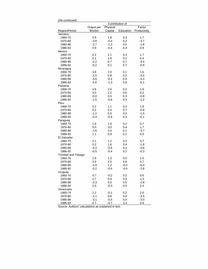
(A6 continued)Contribution of:

FactorPhysicalOutput perProductivityEducationCapitalWorkerRegion/Period

Jamaica1.70.31.83.9 1960-70-3.70.2-0.3-3.8 1970-80-1.80.5-1.3-2.7 1980-860.80.4-0.40.9 1986-92

Mexico1.70.42.14.2 1960-700.40.11.62.1 1970-80-3.50.70.7-2.2 1980-86-0.90.70.1-0.2 1986-92

Nicaragua1.60.12.03.8 1960-70-3.50.20.8-2.5 1970-80-4.30.9-0.2-3.6 1980-86-5.10.8-1.3-5.6 1986-92

Panama1.90.22.64.8 1960-700.20.62.23.0 1970-80-0.80.30.5-0.0 1980-86-1.20.3-0.6-1.5 1986-92

Peru1.80.31.13.2 1960-70-0.90.70.30.2 1970-80-1.50.30.0-1.2 1980-86-5.10.3-0.6-5.4 1986-92

Paraguay0.70.21.01.9 1960-701.70.43.05.0 1970-80-3.70.12.0-1.6 1980-860.00.10.91.1 1986-92

El Salvador0.70.21.22.1 1960-70-1.80.41.60.2 1970-80-3.80.2-0.6-4.2 1980-86-0.30.2-0.4-0.5 1986-92

Trinidad and Tobago1.50.01.32.9 1960-700.70.62.53.9 1970-80-6.0-0.01.2-4.9 1980-86-2.8-0.0-0.4-3.2 1986-92

Uruguay0.60.2-0.20.7 1960-701.30.40.92.7 1970-80-2.80.50.0-2.3 1980-862.40.5-0.32.5 1986-92

Venezuela2.00.2-0.12.2 1960-70-3.50.90.6-2.1 1970-80-3.00.4-0.5-3.1 1980-860.90.4-0.70.7 1986-92

Source: Authors' calculations as explained in text.

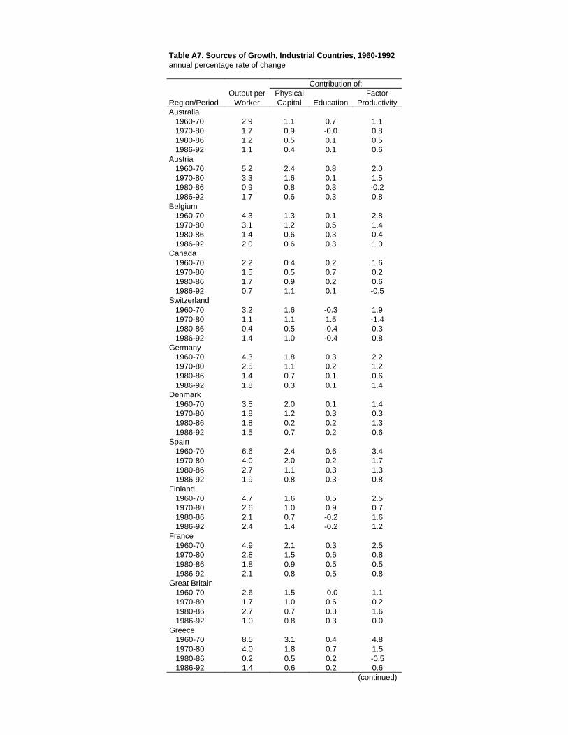
Table A7. Sources of Growth, Industrial Countries, 1960-1992annual percentage rate of change

Contribution of:FactorPhysicalOutput per

ProductivityEducationCapitalWorkerRegion/PeriodAustralia

1.10.71.12.9 1960-700.8-0.00.91.7 1970-800.50.10.51.2 1980-860.60.10.41.1 1986-92

Austria2.00.82.45.2 1960-701.50.11.63.3 1970-80-0.20.30.80.9 1980-860.80.30.61.7 1986-92

Belgium2.80.11.34.3 1960-701.40.51.23.1 1970-800.40.30.61.4 1980-861.00.30.62.0 1986-92

Canada1.60.20.42.2 1960-700.20.70.51.5 1970-800.60.20.91.7 1980-86-0.50.11.10.7 1986-92

Switzerland1.9-0.31.63.2 1960-70-1.41.51.11.1 1970-800.3-0.40.50.4 1980-860.8-0.41.01.4 1986-92

Germany2.20.31.84.3 1960-701.20.21.12.5 1970-800.60.10.71.4 1980-861.40.10.31.8 1986-92

Denmark1.40.12.03.5 1960-700.30.31.21.8 1970-801.30.20.21.8 1980-860.60.20.71.5 1986-92

Spain3.40.62.46.6 1960-701.70.22.04.0 1970-801.30.31.12.7 1980-860.80.30.81.9 1986-92

Finland 2.50.51.64.7 1960-700.70.91.02.6 1970-801.6-0.20.72.1 1980-861.2-0.21.42.4 1986-92

France2.50.32.14.9 1960-700.80.61.52.8 1970-800.50.50.91.8 1980-860.80.50.82.1 1986-92

Great Britain1.1-0.01.52.6 1960-700.20.61.01.7 1970-801.60.30.72.7 1980-860.00.30.81.0 1986-92

Greece4.80.43.18.5 1960-701.50.71.84.0 1970-80-0.50.20.50.2 1980-860.60.20.61.4 1986-92

(continued)

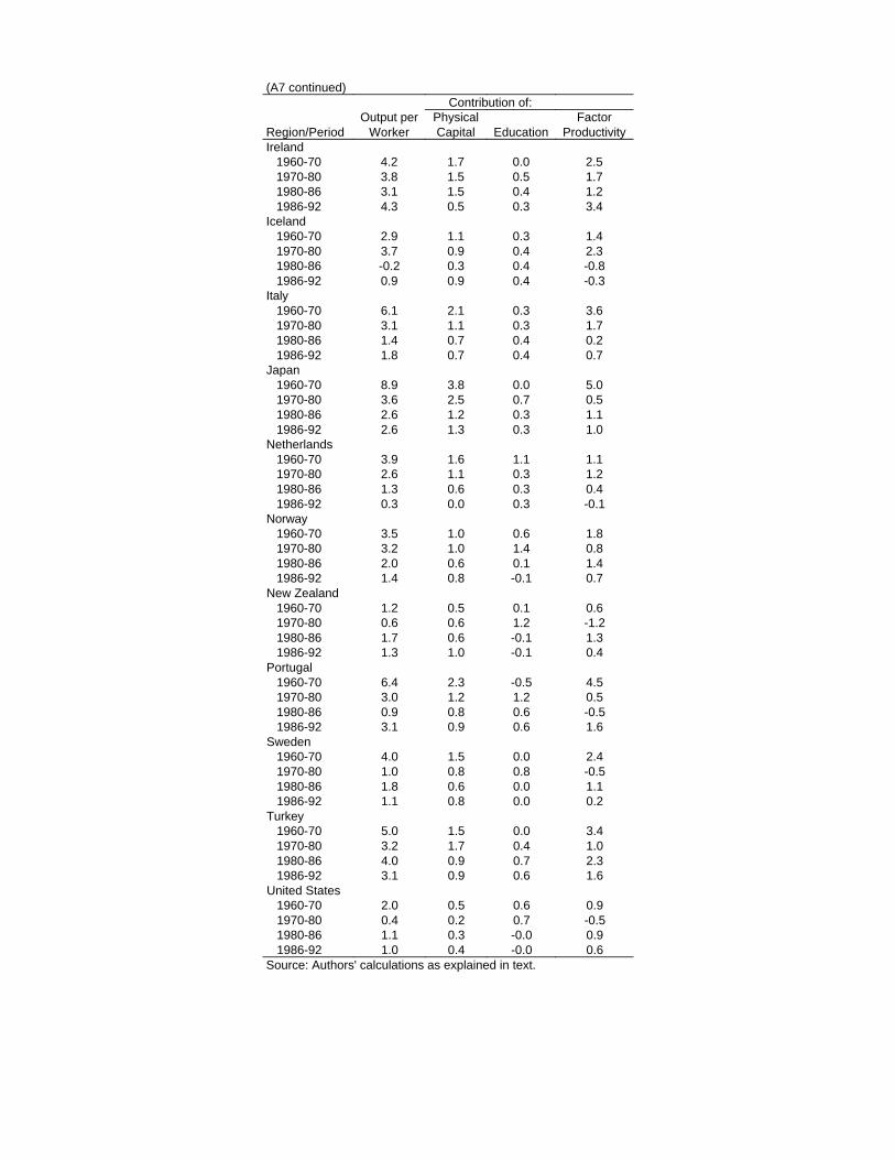
(A7 continued)Contribution of:

FactorPhysicalOutput perProductivityEducationCapitalWorkerRegion/Period

Ireland2.50.01.74.2 1960-701.70.51.53.8 1970-801.20.41.53.1 1980-863.40.30.54.3 1986-92

Iceland1.40.31.12.9 1960-702.30.40.93.7 1970-80-0.80.40.3-0.2 1980-86-0.30.40.90.9 1986-92

Italy3.60.32.16.1 1960-701.70.31.13.1 1970-800.20.40.71.4 1980-860.70.40.71.8 1986-92

Japan5.00.03.88.9 1960-700.50.72.53.6 1970-801.10.31.22.6 1980-861.00.31.32.6 1986-92

Netherlands1.11.11.63.9 1960-701.20.31.12.6 1970-800.40.30.61.3 1980-86-0.10.30.00.3 1986-92

Norway1.80.61.03.5 1960-700.81.41.03.2 1970-801.40.10.62.0 1980-860.7-0.10.81.4 1986-92

New Zealand0.60.10.51.2 1960-70-1.21.20.60.6 1970-801.3-0.10.61.7 1980-860.4-0.11.01.3 1986-92

Portugal4.5-0.52.36.4 1960-700.51.21.23.0 1970-80-0.50.60.80.9 1980-861.60.60.93.1 1986-92

Sweden2.40.01.54.0 1960-70-0.50.80.81.0 1970-801.10.00.61.8 1980-860.20.00.81.1 1986-92

Turkey3.40.01.55.0 1960-701.00.41.73.2 1970-802.30.70.94.0 1980-861.60.60.93.1 1986-92

United States0.90.60.52.0 1960-70-0.50.70.20.4 1970-800.9-0.00.31.1 1980-860.6-0.00.41.0 1986-92

Source: Authors' calculations as explained in text.

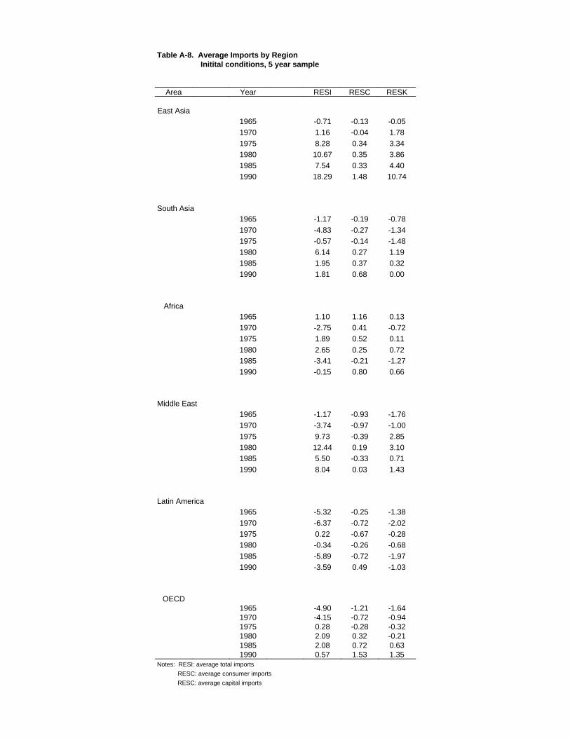
Table A-8. Average Imports by Region Initital conditions, 5 year sample

RESKRESCRESIYearArea

East Asia-0.05-0.13-0.7119651.78-0.041.1619703.340.348.2819753.860.3510.6719804.400.337.54198510.741.4818.291990

South Asia-0.78-0.19-1.171965-1.34-0.27-4.831970-1.48-0.14-0.5719751.190.276.1419800.320.371.9519850.000.681.811990

Africa0.131.161.101965-0.720.41-2.7519700.110.521.8919750.720.252.651980-1.27-0.21-3.4119850.660.80-0.151990

Middle East-1.76-0.93-1.171965-1.00-0.97-3.7419702.85-0.399.7319753.100.1912.4419800.71-0.335.5019851.430.038.041990

Latin America-1.38-0.25-5.321965-2.02-0.72-6.371970-0.28-0.670.221975-0.68-0.26-0.341980-1.97-0.72-5.891985-1.030.49-3.591990

OECD-1.64-1.21-4.901965-0.94-0.72-4.151970-0.32-0.280.281975-0.210.322.0919800.630.722.0819851.351.530.571990

Notes: RESI: average total imports

RESC: average consumer imports

RESC: average capital imports