decay of entropy from a conservative spectral method for ... boltzmann and landau equations,...
TRANSCRIPT

Decay of Entropy From a Conservative Spectral Method forFokker-Planck-Landau Type Equations
Clark A. Pennie1,a) and Irene M. Gamba1,b)
1The University of Texas at Austin, Austin, TX 78712, USA
a)Corresponding author: [email protected])[email protected]
Abstract. Expanding upon the conservative spectral method for solving the Landau equation, developed by Zhang and Gamba, adeterministic scheme has been developed for modeling Fokker-Planck-Landau type equations with Maxwell molecules and hardsphere interactions. The original case, corresponding to the classical physical problem of Coulomb interactions, is also includedand the stability for all three scenarios investigated. The power of the method is exemplified through simulations demonstrating thedecay of relative entropy for both Coulomb interactions and hard potentials. The Coulomb interaction example shows that there isa degenerate spectrum, with the relative entropy decaying at a rate close to the law of two thirds as predicted by Strain and Guo,while the hard potential example exhibits a spectral gap.
1 Introduction
An important model for plasmas is the Landau equation, which results from the grazing collision limit of the Boltz-mann equation. This limit, first derived by Landau [1], assumes that colliding particles are travelling almost parallelto each other due to repulsive Coulomb forces. A more mathematical description of the limit was detailed by Villani[2] and Desvillettes and Villani [3], even for extended potential rates higher than Coulumb interactions and up tohard spheres. When rates different to Coulomb interactions are used, the equation is referred to as being of Fokker-Planck-Landau type. Computationally, the problem has been studied by Bobylev and Potapenko [4], using MonteCarlo methods, and in Fourier space by Haack and Gamba [5].
The Landau equation is rather difficult to model, either analytically or numerically, due to the high dimensionality,non-linearity and non-locality. For numerical simulations, a deterministic scheme can be used, such as the conservativespectral method, developed by Zhang and Gamba [6], which is the model of choice for the current work. Spectralmethods were first considered as a model for the homogeneous Landau equation by Bobylev and Rjasanow [7] andPareschi et al. [8]. The evolution of the Landau equation has also been simulated by means of a Monte-Carlo schemefor the Boltzmann equation with sufficiently singular angular cross-sections that cancel the Coulomb potential. Thisapproach results in an expensive algorithm compared to the spectral-based methods.
The version of the spectral method in this work exploits the weak form of the Landau equation in order tocalculate the Fourier transform of the collision operator. It does so in justO(N3 log N) operations, where the number ofFourier modes N in each velocity dimension can be small, thanks to the conservation enforcement. For computationalpurposes, a cut-off domain in velocity space is used, within which the majority of the solution’s mass should besupported, based on a result by Gamba et al. [9] for the Boltzmann equation. This general construction of a spectralmethod was first applied to the Boltzmann equation by Gamba and Tharkabhushaman [10] and the details for thederivation of the Landau equation scheme can be found in [6].
Pareschi’s construction of a spectral method involved extending the solution periodically, which did not respectthe decay of the solution toward infinity in velocity space. As a result, aliasing effects were noticed in their solution.Subsequently, Filbet and Pareschi [11] applied this idea to the inhomogeneous Landau equation by using a finitevolume method in space but this scheme did not preserve the conservation properties of the Landau equation. Aconservative method was later proposed by Crouseilles and Filbet [12], using centered finite differences, but this onlyconserved mass and energy, not momentum, and required certain symmetry properties of the initial data.

One particular attraction to the current method is its ability to yield the correct decay of entropy. The conservationenforcement is essential in the proof of convergence of the spectral method applied to the Boltzmann equation [13]and it is believed that the same should be true for Fokker-Planck-Landau type equations. The entropy decay rate isalso a consequence of this fact. To the best of the authors’ knowledge, this is the first time that the convergence rateof two thirds, proven analytically by Strain and Guo [14], has been seen through a numerical approximation of therelative entropy.
The method described in [6] is in fact a solver for the inhomogeneous Landau equation, coupled to Poisson’sequation, where the advection is modeled by a discontinuous Galerkin scheme. Extensions of the relative entropyresults in this work to the inhomogeneous case are in progress. In addition, this paper contains results for Fokker-Planck-Landau type equations associated to Maxwell molecules and hard spheres, expanding upon the previous work.
The layout of this work is as follows. First, the set up of the problem is described in section 2, along with anyrequired definitions. The expressions for the Fourier transform of the Fokker-Planck-Landau type operators corre-sponding to Coulomb interactions, Maxwell molecules and hard spheres are derived in section 3 and the stabilityresults given in section 4. Finally, section 5 contains the numerical results, demonstrating the correct decay rate toequilibrium for both Coulomb interactions and hard spheres. All work here is part of a PhD thesis by the first author,under advisorship of the second, and elaborated on in a future work by both authors [15].
2 Description of Problem
A space-homogeneous Fokker-Planck-Landau type equation for the probability density function (pdf) f (t, v), where(t, v) ∈ (R+,Ωv), with Ωv ⊆ R3, is of the form
ft(t, v) =1ε
Q( f , f )(t, v), (1)
where ε is the Knudsen number and Q( f , f ) is the collision operator given by
Q( f , f ) = ∇v ·
∫Ωv
S (v − v∗)( f∗∇v f − f∇v∗ f∗) dv∗, for S (u) = |u|γ+2(I −
uuT
|u|2
),
with −3 ≤ γ ≤ 1, I ∈ R3×3 the identity matrix and the subscript notation f∗ meaning evaluation at v∗. In general, γ > 0corresponds to hard potentials and γ < 0 to soft potentials. In particular, γ = 1 model hard spheres; γ = 0 are knownas Maxwell molecules; and γ = −3 model Coulomb interactions between particles.
Since Fokker-Planck-Landau type equations are a limit of the Boltzmann equation, they enjoy the same conser-vation laws. In particular, for the set of collision invariants φk(v)4k=0 =
1, v1, v2, v3, |v|2
,∫
R3Q( f , f )(v)φk(v) dv = 0, for k = 0, 1, . . . , 4. (2)
This is important because it leads to the conservation of mass ρ, average velocity V and temperature T , where each ofthese quantities are found via
ρ =
∫R3
f (t, v) dv, V =1ρ
∫R3
f (t, v)v dv and T =1
3ρ
∫R3
f (t, v)|v − V|2 dv.
These moments will always be conserved for the single-species homogeneous Landau equation (1) as well as forthe corresponding space-inhomogenous version, if modeled with appropriate boundary conditions (e.g. reflective orperiodic boundary conditions).
If the initial mass, average velocity and temperature are denoted by ρ0, V0 and T0, respectively, the equilibriumsolution of the Landau equation is a Gaussian distribution with the same moments. This is referred to as the equilibriumMaxwellian, denoted byMeq, and is the specific Maxwellian distribution with moments equal to those of the initialcondition, given by
Meq(v) =ρ0
(2πT0)32
e−|v−V0 |
2
2T0 .

Similarly, the H-theorem holds for Fokker-Planck-Landau type equations, which states that the entropy decaysthroughout time.
The entropy is defined as H[ f ](t) =
∫R3
f log( f ) dv
and so the H-theorem gives thatddt
(H[ f ]) ≤ 0.
At this point it is also useful to define the entropy relative to the equilibrium MaxwellianMeq as
H[ f |Meq](t) =
∫R3
f log( f ) dv −∫R3Meq log(Meq) dv =
∫R3
f log(
fMeq
)dv. (3)
Initially f (0, v) = f0(v) and it is assumed that supp f b Ωv, since f should have sufficient decay in velocity-space[9] and Ωv is chosen depending on the initial data (see [13], section 2). In fact, v ∈ R3 but values of f are negligibleoutside a sufficiently large ball. The initial data is then extended by zero outside the computational domain, whichmeans it can be controlled by e−c|v|2 , for c > 0 depending on the moments of f0. Under such conditions, it is expectedthat the computational solution will remain supported on Ωv up to a fixed small error that depends on the initial data(more details can be seen in the proof for the conservative spectral method applied to the Boltzmann equation in [13]).
Equation (1) is solved by the conservative spectral method with fourth order Runge-Kutta for time-stepping.Conservation is enforced by considering a constrained minimisation problem. Given a collection of discrete values ofthe collision operator, resulting from the spectral method, a new set of values must be found which are as close aspossible to the original values in `2-norm but satisfy the discrete form of (2), where the integrals are replaced withquadrature sums. The solution to this problem is a matrix multiplication of the original values, where the matrix isidentical for both the Boltzmann and Landau equations. The complete derivation can be found in [10] and [6] forthe Boltzmann and Landau equations, respectively. As will be seen in the current work, the method also respects thecorrect decay rate of entropy. The spectral method will be described in the next section and is extended from theLandau equation with Coulomb interactions to Fokker-Planck-Landau type equations with Maxwell molecule andhard sphere interactions.
3 The Fourier Transform of the Collision Operator
As is shown in [6], when using a ball of radius R > 0 as the cut-off domain for computational purposes, the Fouriertransform of the collision operator Q is
Q( f , f ) (ξ) =
∫Ωξ
f (ξ − ω) f (ω)(ωT S (ω)ω − (ξ − ω)T S (ω) (ξ − ω)
)dω, for ξ ∈ Ωξ ⊆ R3, (4)
where S (ω) = (2π)−32
∫BR(0)
S (u)e−iω·udu, for S (u) = |u|γ+2(I −
uuT
|u|2
), with − 3 ≤ γ ≤ 1.
This means that evaluating Q is performed by a fast Fourier transform (FFT) of the pdf f and then a weightedconvolution with itself. The FFT requires O(N3 log N) operations and multiplication by the weight and quadrature tocalculate the convolution requiresO(N3) operations. The weights can also be pre-computed and stored at the beginningof the code run, where the bulk of the calculation is in evaluation of S . This has different forms depending on the valueof γ but the results are found through the same general method.
First, the entries of S can be decomposed as S i, j(ω) = S 1i, j(ω) − S 2
i, j(ω), for i, j = 1, 2, 3, with
S 1i, j(ω) = (2π)−
32
∫BR(0)|u|γ+2δi, je−iω·u du and S 2
i, j(ω) = (2π)−32
∫BR(0)|u|γuiu je−iω·u du. (5)
Then, for a given ω = (ω1, ω2, ω3), it should be noted that when j = i, there is only one value of S 1i,i(ω), for each
i = 1, 2, 3, and that S 1i, j(ω) = 0 when i , j (thanks to the Kronecker delta). Also note that
S 21,1(ω1, ω2, ω3) = S 2
3,3(ω2, ω3, ω1) and S 22,2(ω1, ω2, ω3) = S 2
3,3(ω1, ω3, ω2), for i = j
and S 21,2(ω1, ω2, ω3) = S 2
1,3(ω1, ω3, ω2) and S 22,3(ω1, ω2, ω3) = S 2
1,3(ω2, ω1, ω3), for i , j.
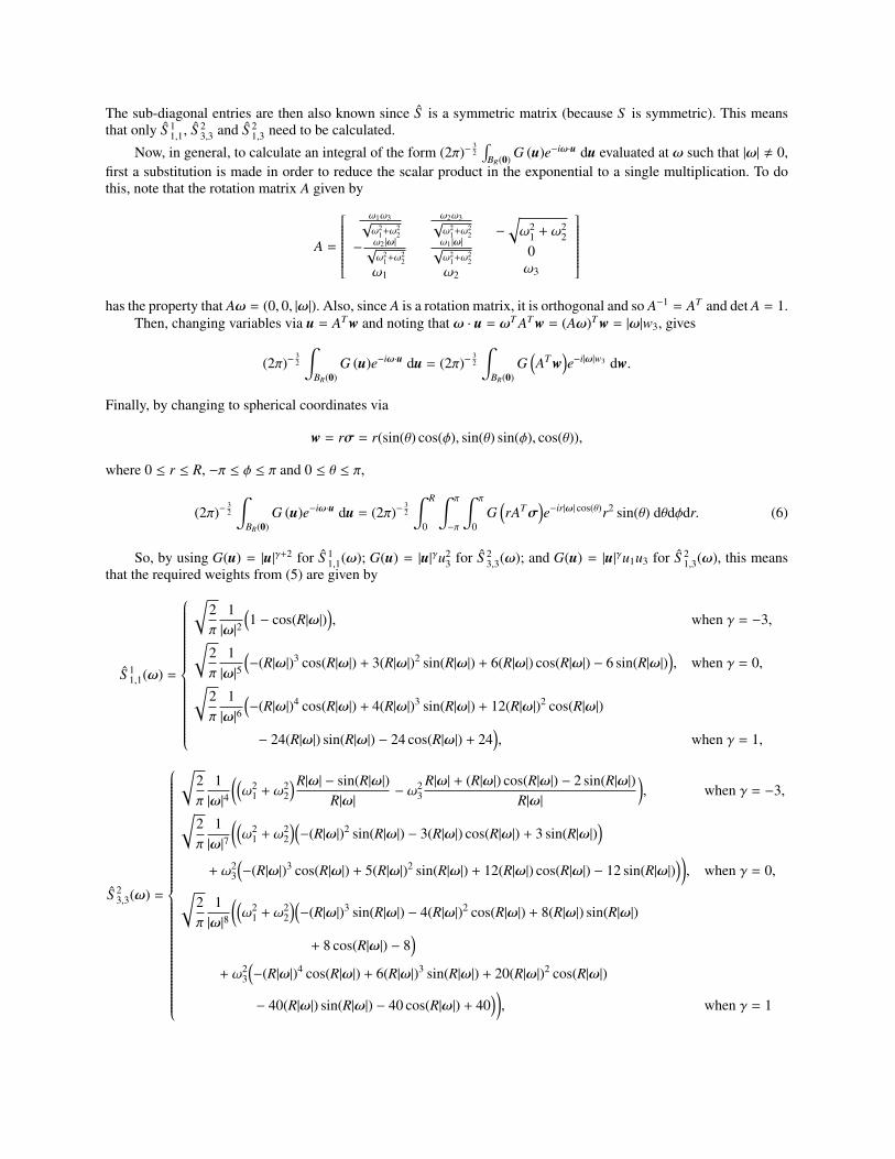
The sub-diagonal entries are then also known since S is a symmetric matrix (because S is symmetric). This meansthat only S 1
1,1, S 23,3 and S 2
1,3 need to be calculated.
Now, in general, to calculate an integral of the form (2π)−32
∫BR(0) G (u)e−iω·u du evaluated at ω such that |ω| , 0,
first a substitution is made in order to reduce the scalar product in the exponential to a single multiplication. To dothis, note that the rotation matrix A given by
A =
ω1ω3√ω2
1+ω22
−ω2 |ω|√ω2
1+ω22
ω1
ω2ω3√ω2
1+ω22
ω1 |ω|√ω2
1+ω22
ω2
−
√ω2
1 + ω22
0ω3
has the property that Aω = (0, 0, |ω|). Also, since A is a rotation matrix, it is orthogonal and so A−1 = AT and det A = 1.
Then, changing variables via u = AT w and noting that ω · u = ωT AT w = (Aω)T w = |ω|w3, gives
(2π)−32
∫BR(0)
G (u)e−iω·u du = (2π)−32
∫BR(0)
G(AT w
)e−i|ω|w3 dw.
Finally, by changing to spherical coordinates via
w = rσ = r(sin(θ) cos(φ), sin(θ) sin(φ), cos(θ)),
where 0 ≤ r ≤ R, −π ≤ φ ≤ π and 0 ≤ θ ≤ π,
(2π)−32
∫BR(0)
G (u)e−iω·u du = (2π)−32
∫ R
0
∫ π
−π
∫ π
0G
(rATσ
)e−ir|ω| cos(θ)r2 sin(θ) dθdφdr. (6)
So, by using G(u) = |u|γ+2 for S 11,1(ω); G(u) = |u|γu2
3 for S 23,3(ω); and G(u) = |u|γu1u3 for S 2
1,3(ω), this meansthat the required weights from (5) are given by
S 11,1(ω) =
√2π
1|ω|2
(1 − cos(R|ω|)
), when γ = −3,√
2π
1|ω|5
(−(R|ω|)3 cos(R|ω|) + 3(R|ω|)2 sin(R|ω|) + 6(R|ω|) cos(R|ω|) − 6 sin(R|ω|)
), when γ = 0,√
2π
1|ω|6
(−(R|ω|)4 cos(R|ω|) + 4(R|ω|)3 sin(R|ω|) + 12(R|ω|)2 cos(R|ω|)
− 24(R|ω|) sin(R|ω|) − 24 cos(R|ω|) + 24), when γ = 1,
S 23,3(ω) =
√2π
1|ω|4
((ω2
1 + ω22
)R|ω| − sin(R|ω|)R|ω|
− ω23
R|ω| + (R|ω|) cos(R|ω|) − 2 sin(R|ω|)R|ω|
), when γ = −3,√
2π
1|ω|7
((ω2
1 + ω22
)(−(R|ω|)2 sin(R|ω|) − 3(R|ω|) cos(R|ω|) + 3 sin(R|ω|)
)+ ω2
3
(−(R|ω|)3 cos(R|ω|) + 5(R|ω|)2 sin(R|ω|) + 12(R|ω|) cos(R|ω|) − 12 sin(R|ω|)
)), when γ = 0,√
2π
1|ω|8
((ω2
1 + ω22
)(−(R|ω|)3 sin(R|ω|) − 4(R|ω|)2 cos(R|ω|) + 8(R|ω|) sin(R|ω|)
+ 8 cos(R|ω|) − 8)
+ ω23
(−(R|ω|)4 cos(R|ω|) + 6(R|ω|)3 sin(R|ω|) + 20(R|ω|)2 cos(R|ω|)
− 40(R|ω|) sin(R|ω|) − 40 cos(R|ω|) + 40)), when γ = 1

and
S 21,3(ω) =
−
√2π
ω1ω3
|ω|42R|ω| + R|ω| cos(R|ω|) − 3 sin(R|ω|)
R|ω|, when γ = −3,√
2π
ω1ω3
|ω|7
(−(R|ω|)3 cos(R|ω|) + 6(R|ω|)2 sin(R|ω|) + 15(R|ω|) cos(R|ω|) − 15 sin(R|ω|)
), when γ = 0,√
2π
ω1ω3
|ω|8
(−(R|ω|)4 cos(R|ω|) + 7(R|ω|)3 sin(R|ω|) + 24(R|ω|)2 cos(R|ω|)
− 48(R|ω|) sin(R|ω|) − 48 cos(R|ω|) + 48), when γ = 1.
In addition, by substituting ω = 0 into the integrands found in S 11,1, S 2
3,3 and S 21,3 from (5) and evaluating directly
(noting that the exponential evaluated at ω = 0 is equal to one),
S 11,1(0) =
√1
2πR2, when γ = −3,
25
√1
2πR5, when γ = 0,
13
√1
2πR6, when γ = 1,
S 23,3(0) =
1
3√
2πR2, when γ = −3,
2
15√
2πR5, when γ = 0,
1
9√
2πR6, when γ = 1
and S 21,3(0) = 0 (for all γ).
4 Stability of the Space-homogeneous Spectral Method
In order to consider the stability of the spectral method, first note that the integral (4) to calculate Q is approximatedusing quadrature. The current code uses the composite trapezoidal rule but, in general, for M equally spaced quadraturenodes ξm
Mm=1 in Fourier space, corresponding weights wm
Mm=1 and Fourier space stepsize hξ,
Q(ξk
)= h3
ξ
M∑m=1
wm f(ξk − ξm
)f (ξm)
(ξm
T S(ξm
)ξm −
(ξk − ξm
)T S(ξm
) (ξk − ξm
)), (7)
Now, according to Lebedev [16], the criterion for stability of a numerical method of the form
ddt
(f (ξk)
)= F( f (ξk))
is that the time-stepsize ∆t must satisfy ∆t ≤1
Lip(F),
for the Lipschitz norm of F, Lip(F). If an upper bound can be found on Lip(F), this will in turn give a lower boundon (Lip(F))−1, which ∆t must be below for the numerical method to remain stable. To find the upper bound, note that
Lip(F) ≤ |Jk,l|, for the Jacobian Jk,l of F( f (ξk)), given by Jk,l =∂
∂ f (ξl)
(F( f (ξk))
).
Here, F( f (ξk)) = 1εQ( f , f )
(ξk
)and, to calculate the derivative of Q( f , f )
(ξk
)with respect to f (ξl), it should be
noted that there are two chances for f (ξl) to appear in the quadrature sum (7). These are when m = l and in general(depending on the choice of quadrature nodes) at another index, say m = n, where ξk−ξn = ξl. Assuming that there areindeed two indices which give rise to non-zero derivatives in the sum, and considering that ξk − ξn = ξl is equivalentto ξn = ξk − ξl, the derivative is given by
∂
∂ f (ξl)
(Q( f , f )
(ξk
))= h3
ξwl f(ξk − ξl
) (ξl
T S(ξl)ξl −
(ξk − ξl
)T S(ξl) (ξk − ξl
))+ h3
ξwn f(ξn
) (ξn
T S(ξn
)ξn −
(ξk − ξn
)T S(ξn
) (ξk − ξn
))= h3
ξwl f(ξk − ξl
) (ξl
T S(ξl)ξl −
(ξk − ξl
)T S(ξl) (ξk − ξl
))+ h3
ξwn f(ξk − ξl
) ((ξk − ξl)
T S(ξk − ξl
)(ξk − ξl) − ξ
Tl S
(ξk − ξl
)ξl
). (8)

Then, since hξ = πLv
and |wl| ≤ 1 for any l, by the triangle inequality,∣∣∣∣∣∣ ∂
∂ f (ξl)
(Q( f , f )
(ξk
))∣∣∣∣∣∣ ≤ π3
L3v| f
(ξk − ξl
)|(|ξl
T S(ξl)ξl| + |
(ξk − ξl
)T S(ξl) (ξk − ξl
)|
+ |(ξk − ξl)T S
(ξk − ξl
)(ξk − ξl)| + |ξ
Tl S
(ξk − ξl
)ξl|
).
Note that if there had been no such ξn then the final two terms would be omitted here and the bound would only besmaller.
Also, by definition of the Fourier transform,
| f(ξk − ξl
)| ≤ (2π)−
32
∫BR(0)| f (u) ||e−i(ξk−ξl)·u|du = (2π)−
32 || f ||L1(BR(0)),
since |e−i(ξk−ξl)·u| = 1, and so∣∣∣∣∣∣ ∂
∂ f (ξl)
(Q( f , f )
(ξk
))∣∣∣∣∣∣ ≤ π32
2√
2L3v
|| f ||L1(BR(0))
(|ξl
T S(ξl)ξl| + |
(ξk − ξl
)T S(ξl) (ξk − ξl
)|
+ |(ξk − ξl)T S
(ξk − ξl
)(ξk − ξl)| + |ξ
Tl S
(ξk − ξl
)ξl|
). (9)
Now, for the terms involving S , note that for a general matrix A ∈ R3×3 and vectors y, z ∈ R3,
yT Az =
3∑i, j=1
Ai, jyiz j and so |yT Az| ≤ (3)2 maxi, j=1,2,3
|Ai, j|( maxi=1,2,3
yi)( maxi=1,2,3
zi). (10)
This means that a bound must be found on |S i, j(ξ)|, which is achieved by using the expressions in section 3 for S 11,1,
S 23,3 and S 2
1,3, for γ = −3, 0 and 1. It is shown in [15] that, for any k = 1, 2, . . . ,M,
|S i, j(ξk)| ≤
(√1
2π+
3π3
(π + 1
)√2π
)L2
v , when γ = −3,√2π
1π5
(2π3 + 9π2 + 21π + 21
)L5
v , when γ = 0,√2π
1π6
(2π6 + 11π3 + 36π2 + 72π + 144
)L6
v , when γ = 1
.
L2
v , when γ = −3,
L5v , when γ = 0,
L6v , when γ = 1.
Then, by using the identity (10) and noting that |(ξk)i| ≤ Lξ = πhv
, for any k, l, n = 1, 2, . . . ,M,
|ξTk S (ξl)ξn| . 9
π2
h2v×
L2
v , when γ = −3,
L5v , when γ = 0,
L6v , when γ = 1.
Now, since ξk − ξl = ξn, each mixed ξk − ξl and ξl term in inequality (9) has the same upper bound. This gives
∣∣∣∣∣∣ ∂
∂ f (ξl)
(Q( f , f )
(ξk
))∣∣∣∣∣∣ . 4
9 π72
2√
2h2v L3
v
|| f ||L1(BR(0))
×
L2v , when γ = −3,
L5v , when γ = 0,
L6v , when γ = 1,
and so
|Jk,l| ≤1ε
∣∣∣∣∣∣ ∂
∂ f (ξl)
(Q( f , f )
(ξk
))∣∣∣∣∣∣ . 18π72
√2εh2
v
|| f ||L1(BR(0)) ×
1Lv, when γ = −3,
L2v , when γ = 0,
L3v , when γ = 1,
which means
1|Jk,l|
&
√2εLvh2
v
18π72 || f ||L1(BR(0))
, when γ = −3,
√2εh2
v
18π72 L2
v || f ||L1(BR(0)), when γ = 0,
√2εh2
v
18π72 L3
v || f ||L1(BR(0)), when γ = 1.
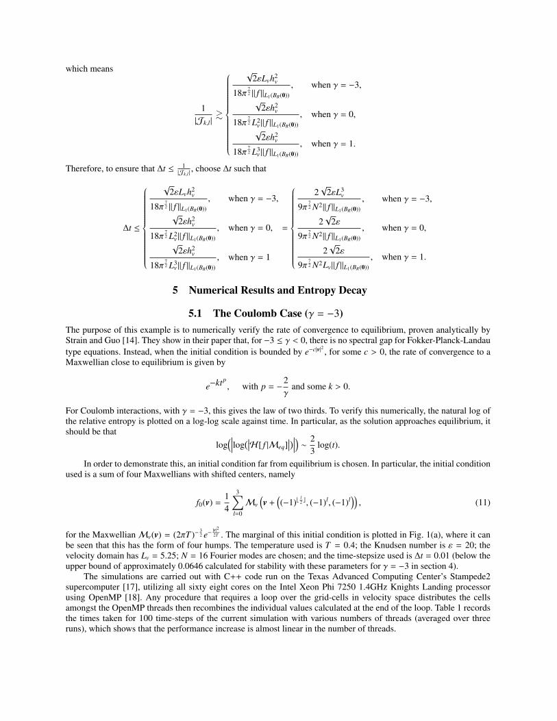
Therefore, to ensure that ∆t ≤ 1|Jk,l |
, choose ∆t such that
∆t ≤
√2εLvh2
v
18π72 || f ||L1(BR(0))
, when γ = −3,
√2εh2
v
18π72 L2
v || f ||L1(BR(0)), when γ = 0,
√2εh2
v
18π72 L3
v || f ||L1(BR(0)), when γ = 1
=
2√
2εL3v
9π72 N2|| f ||L1(BR(0))
, when γ = −3,
2√
2ε
9π72 N2|| f ||L1(BR(0))
, when γ = 0,
2√
2ε
9π72 N2Lv|| f ||L1(BR(0))
, when γ = 1.
5 Numerical Results and Entropy Decay
5.1 The Coulomb Case (γ = −3)The purpose of this example is to numerically verify the rate of convergence to equilibrium, proven analytically byStrain and Guo [14]. They show in their paper that, for −3 ≤ γ < 0, there is no spectral gap for Fokker-Planck-Landautype equations. Instead, when the initial condition is bounded by e−c|v|2 , for some c > 0, the rate of convergence to aMaxwellian close to equilibrium is given by
e−ktp, with p = −
2γ
and some k > 0.
For Coulomb interactions, with γ = −3, this gives the law of two thirds. To verify this numerically, the natural log ofthe relative entropy is plotted on a log-log scale against time. In particular, as the solution approaches equilibrium, itshould be that
log(∣∣∣∣log
(∣∣∣H[ f |Meq]∣∣∣)∣∣∣∣) ∼ 2
3log(t).
In order to demonstrate this, an initial condition far from equilibrium is chosen. In particular, the initial conditionused is a sum of four Maxwellians with shifted centers, namely
f0(v) =14
3∑l=0
Mv
(v +
((−1)b
l2 c, (−1)l, (−1)l
)), (11)
for the MaxwellianMv(v) = (2πT )−32 e−
|v|22T . The marginal of this initial condition is plotted in Fig. 1(a), where it can
be seen that this has the form of four humps. The temperature used is T = 0.4; the Knudsen number is ε = 20; thevelocity domain has Lv = 5.25; N = 16 Fourier modes are chosen; and the time-stepsize used is ∆t = 0.01 (below theupper bound of approximately 0.0646 calculated for stability with these parameters for γ = −3 in section 4).
The simulations are carried out with C++ code run on the Texas Advanced Computing Center’s Stampede2supercomputer [17], utilizing all sixty eight cores on the Intel Xeon Phi 7250 1.4GHz Knights Landing processorusing OpenMP [18]. Any procedure that requires a loop over the grid-cells in velocity space distributes the cellsamongst the OpenMP threads then recombines the individual values calculated at the end of the loop. Table 1 recordsthe times taken for 100 time-steps of the current simulation with various numbers of threads (averaged over threeruns), which shows that the performance increase is almost linear in the number of threads.
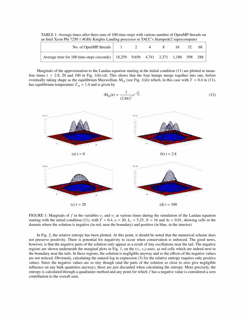
TABLE 1: Average times after three runs of 100 time-steps with various number of OpenMP threads onan Intel Xeon Phi 7250 1.4GHz Knights Landing processor in TACC’s Stampede2 supercomputer
No. of OpenMP threads 1 2 4 8 16 32 68
Average time for 100 time-steps (seconds) 18,259 9,656 4,741 2,371 1,188 598 288
Marginals of the approximation to the Landau equation starting at the initial condition (11) are plotted at mean-free times t = 2.8, 20 and 100 in Fig. 1(b)-(d). This shows that the four humps merge together into one, beforeeventually taking shape as the equilibrium MaxwellianMeq (see Fig. 1(d)) which, in this case with T = 0.4 in (11),has equilibrium temperature Teq = 1.4 and is given by
Meq(v) =1
(2.8π)32
e−|v|22.8 . (12)
(a) t = 0 (b) t = 2.8
(c) t = 20 (d) t = 100
FIGURE 1: Marginals of f in the variables v1 and v2 at various times during the simulation of the Landau equationstarting with the initial condition (11), with T = 0.4, ε = 20, Lv = 5.25, N = 16 and ∆t = 0.01, showing cells in thedomain where the solution is negative (in red, near the boundary) and positive (in blue, in the interior).
In Fig. 2, the relative entropy has been plotted. At this point, it should be noted that the numerical scheme doesnot preserve positivity. There is potential for negativity to occur when conservation is enforced. The good news,however, is that the negative parts of the solution only appear as a result of tiny oscillations near the tail. The negativeregions are shown underneath the marginal plots in Fig. 1, on the (v1, v2)-axes, as red cells which are indeed next tothe boundary near the tails. In these regions, the solution is negligible anyway and so the effects of the negative valuesare not noticed. Obviously, calculating the natural log in expression (3) for the relative entropy requires only positivevalues. Since the negative values are so tiny though (and the parts of the solution so close to zero give negligibleinfluence on any bulk quantities anyway), these are just discarded when calculating the entropy. More precisely, theentropy is calculated through a quadrature method and any point for which f has a negative value is considered a zerocontribution to the overall sum.

When natural logarithms have been taken, the curve does indeed become a straight line when close to equilibrium.It can be seen that, when t = 2.8 (corresponding to Fig. 1(b)), the curve is not yet straight but that is because thesolution is still far from a Maxwellian. At around t = 20 (corresponding to Fig. 1(c)), however, the four humps havedisappeared and the solution is becoming close to that of a Maxwellian. This is part of the entropy plot which is astraight line, with a slope of approximately 0.634, which is fairly close to two thirds, as hoped.
log(t)-5 -4 -3 -2 -1 0 1 2 3 4 5
log(∣ ∣ ∣log(∣ ∣
H[f|M
eq]∣ ∣
)
∣ ∣ ∣
)
-1
-0.5
0
0.5
1
1.5
(a)
(b)
(c)
(d)Relative entropyLine with slope 0.634
FIGURE 2: Plot of log(∣∣∣∣log
(∣∣∣H[ f |Meq]∣∣∣)∣∣∣∣) against log(t) for the numerical approximation f to the Landau equation,
given initial condition (11), with T = 0.4, ε = 20, Lv = 5.25, N = 16 and ∆t = 0.01, which has equilibrium solutionMeq given by (12). A straight line has been added to show that the slope near equilibrium is close to two thirds,exhibiting the lack of spectral gap, but a degenerate spectrum corresponding to a stretch-time exponential decay givenby e−ktp
, with p = 23 and some k > 0. The labels correspond to the marginal plots in Fig. 1.
The importance of the conservation routine should also be noted here. The numerical scheme was run with thesame parameters as above but without enforcing conservation and the deviations of mass and kinetic energy from theirinitial values during this simulation are plotted in Fig. 3(a). When the conservation routine is applied, to produce theresults of Fig. 1-2, the mass and energy were held constant to machine accuracy. Here, however, there is a significantdeviation of O(10−2) showing that there is no hope of convergence to the Maxwellian with the same moments asthe initial data. Nevertheless, a plot of the relative entropy has also been included in Fig. 3(b). Another problemhere is that the entropy in the simulation without conserved moments drops below that of the theoretical equilibriumentropy, resulting in the spike around log(t) ≈ 4.35. There is still an exponential decay of relative entropy, however,as demonstrated by the straight line with a slope of approximately 0.6119. As expected, this is not as accurate as theslope of 0.634 when conservation is enforced.
5.2 The Hard Sphere Case (γ = 1)Unlike when γ < 0, there is a spectral gap when γ = 1. This means the rate of convergence to a Maxwellian close toequilibrium is in fact exponential, of the form e−kt, for some k > 0. Similar to the previous example, when close toequilibrium, the relative entropy should behave like log
(∣∣∣∣log(∣∣∣H[ f |Meq]
∣∣∣)∣∣∣∣) ∼ log(t).Trying to simulate hard spheres introduced a fair amount of difficulty, which shed light on an issue that should
be considered for modeling hard potentials with the current spectral method. In particular, when choosing an initialcondition for which the bulk of the mass is supported in too small a region near the center of the domain, the tails ofthe solution start to ripple after a small number of time-steps, causing an instability which leads to a blow-up. It isbelieved that this problem stems from the fact that collisions are much more significant for hard potentials than softones, with more weight being given to larger relative velocities. The relative velocity becomes larger when closer tothe tails in velocity-space.
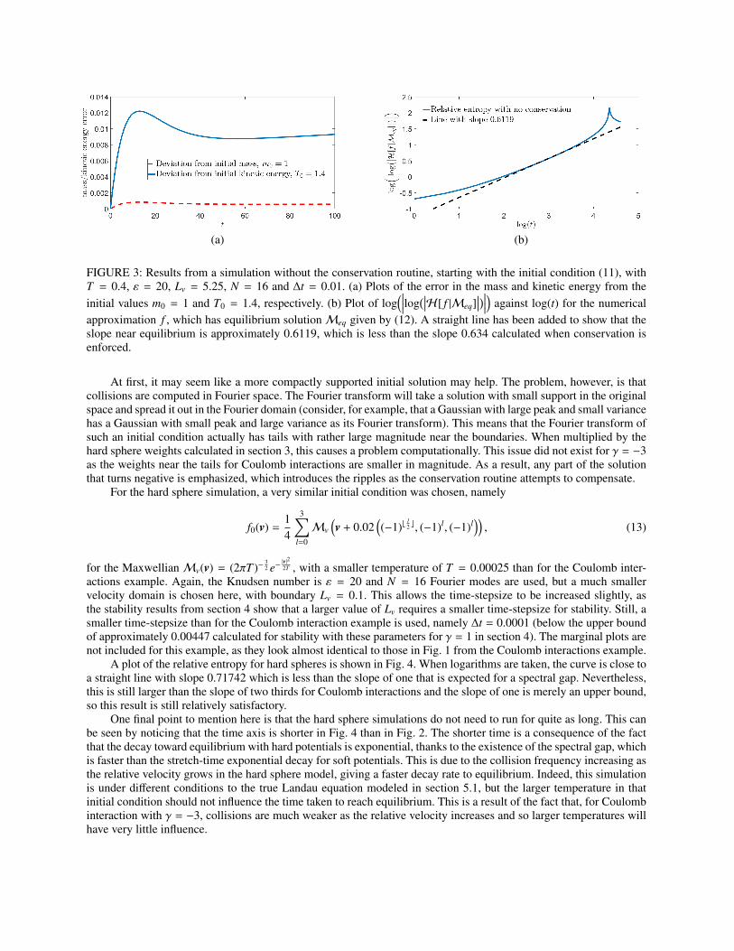
(a) (b)
FIGURE 3: Results from a simulation without the conservation routine, starting with the initial condition (11), withT = 0.4, ε = 20, Lv = 5.25, N = 16 and ∆t = 0.01. (a) Plots of the error in the mass and kinetic energy from theinitial values m0 = 1 and T0 = 1.4, respectively. (b) Plot of log
(∣∣∣∣log(∣∣∣H[ f |Meq]
∣∣∣)∣∣∣∣) against log(t) for the numericalapproximation f , which has equilibrium solutionMeq given by (12). A straight line has been added to show that theslope near equilibrium is approximately 0.6119, which is less than the slope 0.634 calculated when conservation isenforced.
At first, it may seem like a more compactly supported initial solution may help. The problem, however, is thatcollisions are computed in Fourier space. The Fourier transform will take a solution with small support in the originalspace and spread it out in the Fourier domain (consider, for example, that a Gaussian with large peak and small variancehas a Gaussian with small peak and large variance as its Fourier transform). This means that the Fourier transform ofsuch an initial condition actually has tails with rather large magnitude near the boundaries. When multiplied by thehard sphere weights calculated in section 3, this causes a problem computationally. This issue did not exist for γ = −3as the weights near the tails for Coulomb interactions are smaller in magnitude. As a result, any part of the solutionthat turns negative is emphasized, which introduces the ripples as the conservation routine attempts to compensate.
For the hard sphere simulation, a very similar initial condition was chosen, namely
f0(v) =14
3∑l=0
Mv
(v + 0.02
((−1)b
l2 c, (−1)l, (−1)l
)), (13)
for the MaxwellianMv(v) = (2πT )−32 e−
|v|22T , with a smaller temperature of T = 0.00025 than for the Coulomb inter-
actions example. Again, the Knudsen number is ε = 20 and N = 16 Fourier modes are used, but a much smallervelocity domain is chosen here, with boundary Lv = 0.1. This allows the time-stepsize to be increased slightly, asthe stability results from section 4 show that a larger value of Lv requires a smaller time-stepsize for stability. Still, asmaller time-stepsize than for the Coulomb interaction example is used, namely ∆t = 0.0001 (below the upper boundof approximately 0.00447 calculated for stability with these parameters for γ = 1 in section 4). The marginal plots arenot included for this example, as they look almost identical to those in Fig. 1 from the Coulomb interactions example.
A plot of the relative entropy for hard spheres is shown in Fig. 4. When logarithms are taken, the curve is close toa straight line with slope 0.71742 which is less than the slope of one that is expected for a spectral gap. Nevertheless,this is still larger than the slope of two thirds for Coulomb interactions and the slope of one is merely an upper bound,so this result is still relatively satisfactory.
One final point to mention here is that the hard sphere simulations do not need to run for quite as long. This canbe seen by noticing that the time axis is shorter in Fig. 4 than in Fig. 2. The shorter time is a consequence of the factthat the decay toward equilibrium with hard potentials is exponential, thanks to the existence of the spectral gap, whichis faster than the stretch-time exponential decay for soft potentials. This is due to the collision frequency increasing asthe relative velocity grows in the hard sphere model, giving a faster decay rate to equilibrium. Indeed, this simulationis under different conditions to the true Landau equation modeled in section 5.1, but the larger temperature in thatinitial condition should not influence the time taken to reach equilibrium. This is a result of the fact that, for Coulombinteraction with γ = −3, collisions are much weaker as the relative velocity increases and so larger temperatures willhave very little influence.

-5 -4 -3 -2 -1 0 1 2 3 4
0
0.2
0.4
0.6
0.8
1
1.2
1.4
1.6
FIGURE 4: Plot of log(∣∣∣∣log
(∣∣∣H[ f |Meq]∣∣∣)∣∣∣∣) against log(t) for the numerical approximation f to the Fokker-Planck-
Landau type equation with γ = 1 and weights calculated by the exact formulae in section 3, given initial condition(13), with T = 0.00025, ε = 20, Lv = 0.1, N = 16 and ∆t = 0.0001, which has equilibrium solution given by aMaxwellian with temperature Teq = 0.0009750. A straight line has been added to show that the slope near equilibriumis now approximately 0.71742, slightly below the value of one expected for the existence of a spectral gap.
6 Conclusion
In this work, the conservative spectral method for solving space-homogeneous Fokker-Planck-Landau type equationswas expanded upon by extending the calculations to hard spheres and Maxwell molecules. Conditions for stabilitywere then derived for each of the three cases. Finally, examples of the numerical method for Coulomb interactions andhard spheres were given to show the power of the scheme. In particular, the relative entropy during a simulation wasshown to decay close to the correct rate for Coulomb interactions, in accordance with the rate of two thirds predictedby Strain and Guo, which shows that this code is an excellent model for the Landau equation. When the model isapplied to the Fokker-Planck-Landau type equation with hard spheres interactions, the existence of the spectral gapis less evident but it is believed that this result can be improved upon by altering the parameters. The importance ofthe conservation routine was also demonstrated by showing that the decay rate without it is less accurate. Indeed, themethod does not preserve positivity but the regions in which the solution falls below zero are always near the tails andthe solution is negligible there anyway. Clearly this is true as dropping those values in calculation of the entropy didnot detract too much from the result.
The code is easily expandable to the space-inhomogeneous case by use of a discontinuous Galerkin method andtime-splitting. The simulations behave just as expected, also with negligible effects resulting from negative points inthe distribution, and similar decay rates to equilibrium are observed. These results will be featured in an upcomingmanuscript [15]. In addition, work is currently underway to implement the present method in a multi-species setting,based on the calculations by Gamba et al. [19] to develop an asymptotic preserving explicit-implicit numerical schemefor species with disparate masses.
7 ACKNOWLEDGMENTS
The authors would like to thank Chenglong Zhang for help in understanding the code used to implement the conserva-tive spectral method and being available to give advice on any developments. Both authors have been partially fundedby grants from the NSF. The Institute for Computational Engineering Sciences has also been incredibly supportive.

REFERENCES
[1] L. Landau, Phys. Zs. Sov. Union 10, 154–164 (1936).[2] C. Villani, Archive for Rational Mechanics and Analysis 143, 273–307 (1998).[3] L. Desvillettes and C. Villani, Communications in Partial Differential Equations 25, 179–298 (2000).[4] A. Bobylev and I. Potapenko, J. Comput. Phys. 246, 123–144 (2013).[5] J. Haack and I. Gamba, Conservative deterministic spectral Boltzmann solver near the grazing collisions
limit, 28th rarefied gas dynamics conference, AIP Conference Proceedings ( 2012).[6] C. Zhang and I. Gamba, J. Comput. Physics 340, 470–497 (2017).[7] A. Bobylev and S. Rjasanow, Eur. J. Mech. B Fluids 18, 869–887 (1999).[8] L. Pareschi, G. Russo, and G. Toscani, J. Comput. Physics 165, 216–236 (2000).[9] I. Gamba, V. Panferov, and C. Villani, Arch. Rational Mech. Anal. 194, 253–282 (2009).
[10] I. Gamba and S. Tharkabhushaman, J. Comput. Physics 228, 2012–2036 (2009).[11] F. Filbet and L. Pareschi, J. Comput. Physics 179, 1–26 (2002).[12] N. Crouseilles and F. Filbet, J. Comput. Physics 201, 546–572 (2004).[13] R. Alonso, I. Gamba, and S. Tharkabhushaman, SIAM Num. Anal. 56, 3534–3579 (2018).[14] R. Strain and Y. Guo, Arch. Rational Mech. Anal. 187, 287–339 (2008).[15] C. Pennie and I. Gamba, work in progress (2019).[16] V. Lebedev, “How to solve stiff systems of differential equations by explicit methods; numerical methods and
applications (1994),” in Numerical methods and applications (CRC Revivals) 1st ed.[17] The University of Texas at Austin, Texas Advanced Computing Center, http://www.tacc.utexas.edu ( TACC).[18] OpenMP Architecture Review Board, OpenMP Application Program Interface Version 3.0,
http://www.openmp.org/mp-documents/spec30.pdf (May 2008).[19] I. Gamba, S. Jin, and L. Liu, submitted for publication (2018).