decay of dyonic black holes - tata institute of fundamental...
TRANSCRIPT

Decay of dyonic black holes
Rahul Nigam
Department of Theoretical Physics
Tata Institute of Fundamental Research
Mumbai, India.
A thesis submitted for the degree of
Doctor of Philosophy
November, 2008


Declaration
I state that the work, embodied in this thesis, forms my own contribu-
tion to the research work carried out under the guidance of Professor
Sunil Mukhi. I also collaborated with Anindya Mukherjee while he
was a student at TIFR. This work has not been submitted for any
other degree to this or any other University or body. Whenever refer-
ences have been made to previous works of others, it has been clearly
indicated.
(Rahul Nigam)
In my capacity as the supervisor of the candidate’s thesis, I certify
that the above statements are true to the best of my knowledge.
(Sunil Mukhi)


Acknowledgements
Firstly, I would like to thank my advisor, Sunil Mukhi for all his help
during my research span in TIFR. He always supported and guided
me patiently while I was struggling with the new ideas. Discussions
with him were always fun and revealing at the same time. Most
importantly while working with him I learnt that there is always a
solution to every problem, its just one has to look for it at right place
and not to give up before finding it.
I would also like to thank Atish Dabholkar, Avinash Dhar, Gautam
Mandal, Shiraz Minwalla, Sandip Trivedi and Spenta Wadia for all
the help I received from them during my stay in TIFR. They were
always very approachable . Other members of the theory group have
also been very helpful. In particular I would like to thank Deepak
Dhar, Mustansir Barma and Sridhar K. for their help and support.
My collaborator and a good friend Anindya Mukherji has helped me
with stimulating discussions when we were finding it difficult to solve
a problem. I want to thank Debashis Ghoshal, Rajesh Gopakumar
and Ashoke Sen for their help whenever I visited HRI.
I had the good fortune to befriend a lot of students and postdocs in
TIFR. Presence of Costis, Kevin, Lars, Rakesh, Rudra, Sashideep,
Suresh and Suvrat made it a very joyable journey with all the serious
discussions on random topics. I am thankful to Basu, Shamik and
Tridib to patiently answer all my computer related queries. My special
thanks to my friends Anil and Anuradha for their emotional support
and for keeping me updated with the world outside institute.

My thanks are due to the DTP office staff, Raju Bathija, Girish Ogale,
Rajan Pawar and Mohan Shinde who have helped me with any offi-
cial matters. They have always been very friendly. I wish to spe-
cially thank Ajay Salve, our system administrator for his friendship
and prompt help whenever things went wrong with the student room
computers.
Finally I thank my parents and brother for all their love and support.

I dedicate this thesis to my loving parents and brother. I further
dedicate it to all the researchers in India for their sustained
contribution to the field of fundamental sciences.

Contents
1 Introduction 1
2 Decay of Dyonic black holes 7
2.1 Introduction . . . . . . . . . . . . . . . . . . . . . . . . . . . . . . 7
2.2 The system . . . . . . . . . . . . . . . . . . . . . . . . . . . . . . 10
2.3 Decays into a pair of dyons . . . . . . . . . . . . . . . . . . . . . . 12
2.4 Analysis of the marginal stability curves: 12-BPS decay products . 17
2.4.1 Equations of the curves . . . . . . . . . . . . . . . . . . . . 17
2.4.2 Farey fractions and Ford circles . . . . . . . . . . . . . . . 20
2.4.3 Analysis of the decays: Sen circles and Ford circles . . . . 21
2.4.4 Analysis of the decays: higher torsion case . . . . . . . . . 23
2.5 Analysis of the marginal stability curves: 14-BPS decay products . 26
2.5.1 Decays into a 12-BPS and a 1
4-BPS dyon . . . . . . . . . . 26
2.5.2 Decays into two 14-BPS dyons . . . . . . . . . . . . . . . . 27
2.6 Discussion . . . . . . . . . . . . . . . . . . . . . . . . . . . . . . . 31
3 Constraints on “rare” dyon decays 32
3.1 Introduction . . . . . . . . . . . . . . . . . . . . . . . . . . . . . . 32
3.2 Marginal stability for N = 4 dyons . . . . . . . . . . . . . . . . . 34
3.3 Rare dyon decays . . . . . . . . . . . . . . . . . . . . . . . . . . . 37
3.3.1 Analysis and implicit solution . . . . . . . . . . . . . . . . 37
3.3.2 Explicit solution: special cases . . . . . . . . . . . . . . . . 38
3.3.3 General charges, “triangular” moduli . . . . . . . . . . . . 45

CONTENTS
3.3.4 Explicit solution: the general case . . . . . . . . . . . . . . 48
3.4 Multi-particle decays . . . . . . . . . . . . . . . . . . . . . . . . . 50
3.5 Multi-centred black holes . . . . . . . . . . . . . . . . . . . . . . . 51
3.6 Discussion . . . . . . . . . . . . . . . . . . . . . . . . . . . . . . . 58
4 String Networks 59
4.1 String Networks . . . . . . . . . . . . . . . . . . . . . . . . . . . . 59
4.2 Classification of periodic string networks . . . . . . . . . . . . . . 64
4.2.1 Some general properties . . . . . . . . . . . . . . . . . . . 64
4.2.2 Dual grid diagrams . . . . . . . . . . . . . . . . . . . . . . 66
4.2.3 Periodic identifications . . . . . . . . . . . . . . . . . . . . 73
4.3 Discussion . . . . . . . . . . . . . . . . . . . . . . . . . . . . . . . 76
5 Kinematical Analogy for Marginal Dyon Decay 77
5.1 Introduction and review . . . . . . . . . . . . . . . . . . . . . . . 77
5.1.1 Kinematic Analogy . . . . . . . . . . . . . . . . . . . . . . 78
5.1.2 Momentum ellipsoid . . . . . . . . . . . . . . . . . . . . . 82
5.1.3 Multiparticle decays and the issue of codimension . . . . . 84
5.1.4 Decay widths on marginal stability curves . . . . . . . . . 85
6 Conclusions 86
References 91

Chapter 1
Introduction
Black holes in String theory
String theory is a prominent candidate for being the quantum theory of gravity.
The physical idea of this theory is that instead of elementary point like parti-
cles, the most basic building blocks of the nature are string like objects. The
different vibrational modes of these strings give rise to different particles. Ex-
tended objects called “D-Branes” also contribute to the spectrum of the particles
in string theory. Physical consistency requires that a supersymmetric string the-
ory has a 10-dimensional space-time background1. This superstring theory can
still describe a 4 dimensional real world spacetime if we assume that the 6 extra
dimensions are compact, and too small to be detected by present experiments.
Hence a 10-dimensional critical string theory is a quantum theory of supergravity
coupled to supersymmetric matter.
String theory has become a very powerful tool in understanding the very in-
teresting objects known as black holes. Classical black holes are solutions to
Einstein’s equation with very unique properties. Its a region of space in which
the gravitational field is so powerful that nothing, not even electromagnetic ra-
diation, can escape its pull after having fallen past its event horizon. The term
”black hole” derives from the fact that the absorption of visible light renders
the hole’s interior invisible, and indistinguishable from the black space around
1Theories in less than 10d are subcritical and more than 10d are referred to as supercritical.
1

it. While general relativity describes a black hole as a region of empty space
with a point-like singularity at the center and an event horizon at the outer
edge, the description changes when the effects of quantum mechanics are taken
into account.Its been shown that rather than holding captured matter forever,
black holes may slowly leak a form of thermal black body energy called Hawking
radiation and may well have a finite life.
This lead to a striking correspondence between the laws of thermodynamics
and the laws of black hole mechanics. The first law of thermodynamics states that
the variation of the total energy is equal to the temperature times the variation
of the entropy plus the work. The corresponding formula for black hole states
that the variation of the black hole mass is related to the variation of the horizon
area plus the work term proportional to the variation of the all the charges.
δM =κs
2π
δA
4+ µδQ + ΩδJ (1.1)
Consequently, it was shown that the temperature of the black hole is given as
T = κs/2π, κs being the surface gravity.This leads to the identification of the
black hole entropy in terms of the event horizon area,
Smacro =Ahor
4GNh(1.2)
It was shown that the total area of the event horizons of any collection of classical
black holes can never decrease, even if they collide and merge. This is remarkably
similar to the second Law of Thermodynamics, with area playing the role of
entropy.
Although general relativity can be used to perform a semi-classical calcula-
tion of black hole entropy, this situation is theoretically unsatisfying. In statistical
mechanics, entropy is understood as counting the number of microscopic config-
urations of a system which have the same macroscopic qualities(such as mass,
charge, etc.). But without a satisfactory theory of quantum gravity, one cannot
perform such a computation for black holes. However it has been one of the suc-
cesses of string theory that it provides such a microscopic quantum description
for black hole entropy. Black hole is identified with certain states in the spectrum
of string theory and the logarithm of the degeneracy of these states is identified
with the black hole entropy.
2

In string theory, black holes are viewed as a bound state of strings and Dbranes
wrapped around non-contractible cycles of a compact manifold. If gs is the string
coupling constant and N is the order of the number of strings/branes then the
effective perturbation coupling constant is gsN . For N large so that gsN >> 1,
this bound state can gravitate and form a black hole which can be analyzed as
solutions of the low energy effective action. The black hole entropy then can
be computed for this using the Bekenstein-Hawking formula. Now, in the regime
where gsN << 1 and N >> 1, the field theory associated with the strings/branes
bound state becomes weakly coupled and amenable to perturbation. Hence the
degeneracies of various states in the Hilbert space of this theory can be computed
in the weak coupling limit. Now to compare the entropy in two limits we need to
vary gsN gradually from small to large values. However we have no control over
the system for intermediate values of gsN and hence it is not possible to compare
the two limits. This problem can be avoided in a supersymmetric string theory if
we study a certain class of black holes known as BPS black holes. Supersymmetry
provides a lower bound called the Bogomol’nyi-Prasad-Sommerfield bound on the
mass of a state in the theory. For any state, the mass is always greater than or
equal to the central charge in the supersymmetry algebra. The states which
saturate this bound are referred to as BPS states. These states are annihilated
by some subset1 of the total of 16 supercharges and therefore many of their
properties, like mass and degeneracy, are protected under the flow of coupling
constant. In 1996 in a 5-dimensional supersymmetric example, Strominger and
Vafa[2] calculated the leading order degeneracy of the microscopic BPS states and
showed that it was equal to the Bekenstein-Hawking entropy. Subsequent works
in 4-dimensions were performed in this direction and this relation was established
there also.
Black holes which have both electrical and magnetic charges are called dyons.
Extremal dyonic black holes are those that carry minimum mass for a given set
of charges. So, regarding them as states in superstring theory its easy to see that
they saturate the BPS bound, and hence a BPS state which can be counted at
weakly coupling and reliably extrapolated to strong coupling. Therefore counting
1A 1
2-BPS state is annihilated by half of these supercharges while a 1
4-BPS is annihilated
by one-fourth of them.
3

the degeneracy of this class of black hole is an important problem which can give
insight into the non-perturbative aspect of the theory. A degeneracy counting
formula for such an extremal dyonic black hole in four dimensional N = 4 string
theory was proposed by[16] . In this formula, degeneracy is generated by the
inverse of a Siegel modular form of Sp(2, Z). This modular form has well defined
modular transformation properties under the group Sp(2, Z) and is invariant un-
der the subgroup of Sp(2, Z), which is isomorphic to SL(2, Z). The degeneracy
is extracted from this inverse modular form by taking its Fourier transform. The
leading order degeneracy, in the large charge expansion, must be equal to the
Bekenstein-Hawking entropy. The question arises as to what structures in grav-
ity correspond to these subleading terms. This problem is intimately connected
with the idea of curve of marginal stability, as we explain now. The zeroes of the
modular form are poles of the integrand and the residues of these poles cause dis-
crete jumps in the degeneracy formula[10, 11, 14] as we vary the parameters of the
theory. It was argued that this change in degeneracy corresponds to appearance
and disappearance of a two-centered 12-BPS black hole along with the original
single-centered solution. [10, 13, 14, 15] The single-centered solutions exists ev-
erywhere in the moduli space while the two-centered ones can decay on “curves
of marginal stability”. Hence information about curve of marginal stability can
potentially throw light on the various states in string theory that contribute to
the counting formula and their supergravity realization.
A black hole in 4-dimensions is uniquely characterized by it angular momen-
tum,mass and electric and magnetic charges. However we will see that instead
of each charge component, the properties of a black hole depends on certain pa-
rameters which can be constructed out of these charges. These parameters are
invariant under the dualities of the theory and hence play an important role in
defining the entropy. For given electric and magnetic charge vectors qe and qm,
one can combine them as
q =
(qe
qm
)(1.3)
Both qe and qm are Lorentzian vectors which lie in Γ22,6 Narain lattice. There are
three quadratic combinations q2e , q
2m, qe.qm which are invariant under O(22, 6; Z)
4

transformations. It was shown that the partition function that counts the degen-
eracies of dyonic black holes is given in terms of the Igusa cusp form which is a
modular form of weight ten of the group Sp(2, Z). It depends on three complex
variables with a Fourier expansion given by :
1
Φ10(p, q, l)=∑
c(m, n, l)pmqnyl (1.4)
Where sum is over m, n ≥ −1 and l ∈ Z. Then the degeneracies is given in terms
of the Fourier coefficients:
d(Γ) = c(q2e/2, q2
m/2, qe.qm) (1.5)
This calculation requires an integration over a three real dimensional subspace
of the Seigel upper half plane where the integrand involves the inverse of the
above mentioned modular form. However as this integrand develops poles at
different points in the parameter space and whenever these poles are crossed,
the degeneracy picks up an extra contribution. The degeneracy of these black
holes depends on the charges and the moduli fields at infinity. This jump in the
entropy indicated the presence of curves of marginal stability in the moduli space
at which the black holes become marginally stable. These marginal curves were
studied in detail for the case where product black holes were both 12BPS[13]. The
curve of marginal stability for this case are of codimension 1.
We studied this phenomenon of marginal dyon decay for the cases where
either one or both of the products were 14BPS. This led to the generalization of
the equation of marginal curve. Since the products have less supersymmetry in
this case, extra constraints have to be imposed on the moduli fields. Because of
the extra constraints the codimension of the curve in this case is two or more
and hence can be avoided in the moduli space. Therefore these decay modes are
called ”rare decays“ and they do not lead to any discrete jumps in the entropy of
the system. We did an intensive study of these rare decay modes and derived the
formula for the marginal curve. We also extended this work to the case where the
original dyon decays into an N-centered dyon. These are also rare decays and do
not change the entropy. We found the maximum codimension of the curve for any
given decay process and our investigation completes the study of a 14-BPS dyon
5

decay. We also discovered a kinematic analogy for the dyon decay phenomenon
and using this analogy we derived the curve of marginal stability in a somewhat
different way.
There is an alternate string network representation to study the dynamics of
a 14BPS dyonic state. It was shown that supersymmetric string theories have a
stable configuration in which three strings of different type meet in a plane. If
the three strings are of type (pi, qi), (1 ≤ i ≤ 3), where p and q are the magnetic
and electric charges respectively, then the charge conservation requires:
3∑
i
pi =
3∑
i
qi = 0 (1.6)
The angles between different strings are adjusted such that the net force on the
vertex due to the tensions between different strings cancel. It Tp,q denotes the
tension of the (p, q) string and ni denotes the direction of the ith string meeting
at the vertex, then we must have
3∑
i
Tp,qni = 0 (1.7)
It was proved that such a configuration satisfies BPS condition. Now given such
a configuration, a string network is constructed by joining many of these vertices
together with above equations satisfied at each vertex. We did a thorough study
of these string networks of arbitrary torsion. The mass of a general dyonic state
can be looked at as a product of the string tension and the length of string
network. We elaborated this geometric way of deriving the mass formula for
a 14BPS dyonic state. The marginal decay of a dyon occurs when one of the
intermediate strings in the network vanishes. The lengths of different strings can
be written as a function of the torus modular parameter. As this length shrinks
to zero, the string network breaks into two disjoint networks. This is exactly
the same process of a 14BPS dyon marginally decaying into two different dyons.
Therefore the constraint which makes the length vanish is same as the constraint
of marginal equation. We further provided a complete classification procedure
for periodic string networks, in the process re-deriving and extending some of the
considerations in Ref.[11].
6

Chapter 2
Decay of Dyonic black holes
In this chapter we study general two-body decays of arbitrary torsion 14-BPS
dyons in four-dimensional type IIB string compactifications. We find a “master
equation” for marginal stability that generalizes the curve found by Sen for 12-
BPS decay, and analyze this equation in a variety of cases including decays to14-BPS products. For 1
2-BPS decays, an interesting and useful relation is exhibited
between walls of marginal stability and the mathematics of Farey sequences and
Ford circles. We exhibit an example in which two curves of marginal stability
intersect in the interior of moduli space.
2.1 Introduction
In the last couple of years there has been renewed interest in the properties of
dyonic black holes in four dimensions, particularly those associated to N = 4
compactifications (type II strings on K3 × T 2 or heterotic/type I strings on T 6,
as well as supersymmetry-preserving orbifolds of these systems) [1, 3, 4, 5, 6, 7,
8, 9, 10, 11, 12, 13, 14, 15]. A key advance has been a better understanding of a
classic degeneracy formula due to Dijkgraaf, Verlinde and Verlinde[16]1.This DVV
counting formula was a conjecture based on some essential requirements that the
answer was required to satisfy, including reduction to the correct formula for
purely electric states, duality invariance and a suitable asymptotic growth. In
1This formula really computes a supersymmetric index, and in what follows when we say
“degeneracy” we will always be referring to this index
7
2.1 Introduction
more recent times this result has been put on a firmer footing by using dualities
involving M-theory, namely the 4d-5d connection[1] and the duality between M-
theory on K3 and the heterotic string[3]. Among other things, the generalization
of this formula to CHL orbifolds and the origin of a genus-2 modular form have
been illuminated in many of these works.
However this formula has been considerably refined from its original form.
To start with any such formula must satisfy the symmetries of the theory. The
symmetry group of the theory under consideration is a 4 dimensional U-duality
group. This can be expressed as the product of a T-duality and a S-duality group.
The T-duality group keeps the norms of the electric charges and magnetic charges
as well as their inner product fixed. While the S-duality group keeps only one
quartic combination of the T-duality invariants fixed. The degeneracy formula is
expressed in terms of the T-duality invariants. S-duality of course changes the
argument of the degeneracy formula but also changes the moduli and the contour
of integration which depends upon the moduli and the T-duality invariants. On
deforming the new contour to the old one a residue corresponding to poles that
the partition function might have, are picked up. Hence degeneracy specification
includes specifying the integration contour in the degeneracy formula and noting
that different contours can lead to different answers for the degeneracy [10, 11].
The effect of varying the integration contours is in the form of discontinuous
jumps in the degeneracy whenever the contour crosses a pole in the integration
variable and picks up the corresponding residue. This has been interpreted as
due to the decay of some 14-BPS dyons into a pair of 1
2-BPS dyons at curves of
marginal stability, which are computed using the BPS mass formula.
Because for large charges the decaying states are black holes, a mechanism
is needed to explain exactly how these decay on curves of marginal stability.
The answer turns out to be [13, 14] that 14-BPS black holes (for a given set of
charges) exist both in single-centre and multi-centre varieties. For the latter, the
separations of the centres are determined by the moduli [25]. If we specialize to
two-centred dyons with both centres being 12-BPS, then it was shown in Ref.[13]
that as we approach a curve of marginal stability the two centres fly apart to
infinity. On the other side of the curve the constraint equation has no solutions.
This explains (in principle, though no method is known to explicitly count states
8

2.1 Introduction
of a two-centred black hole) the phenomenon of marginal stability and jumping in
the counting formula, in terms of the disintegration of two-centred black holes. It
should be noted that the degeneracy of single-centred black holes with the same
charges does not vary across moduli space, therefore they exist either everywhere
or nowhere.
In these developments, the only type of marginal decay that plays a role is
into two 12-BPS final states. Also, the only multi-centred black holes needed to
complete the explanation are those with a pair of 12-BPS centres. Though the
correspondence between these two situations was derived for some special cases,
it is believed to hold in general, namely for any charge vectors and any point in
the entire SL(2)U(1)
× SO(6,22)SO(6)×SO(22)
moduli space of N = 4 compactifications.
Recent work has focused on the issue of marginal stability of these dyons.
Curves of marginal stability for specific decays have been obtained[10], the impact
of such decays on the degeneracy formula has been studied[10, 11, 14] and the
decays across such walls have been identified with the disappearance of two-
centred black holes from the spectrum[13, 14], following previous ideas in the
N = 2 context[17]. A formula has been proposed in [14] to count the “immortal”
dyons which exist everywhere. And very recently, Sen has considered the case
of unit torsion dyons decaying into 14-BPS states[15] and demonstrated that this
takes place only on surfaces of codimension 2 or more in moduli space.
In the present chapter we take a step towards resolving the first problem.
We consider the most general decay of a 14-BPS dyon into two decay products,
each one of which can be either 12- or 1
4-BPS. We find a necessary condition for
marginal two-body decays and study the resulting equation in a variety of cases.
It turns out that some solutions of our equation are “spurious” in the sense that
they describe an inverse decay process rather than the forward decay. This puts
constraints on the possible decay products which are identical to those found in
[15]. We are also able to reproduce some of the results in Refs.[10] as a special
case, as well as generalize them to the case of higher torsion dyons. On the way
we will see that a known mathematical construction, that of Farey sequences and
Ford circles, bears a remarkably close relation to the circles of marginal stability
in Ref.[10] and helps us understand the properties of these circles.
9

2.2 The system
2.2 The system
We consider type IIB string theory first compactified on K3. This is a very
special background, being chiral and half-maximally supersymmetric in six di-
mensions. In this background there are no 1-form gauge fields, and therefore no
BPS particles. However, there are 26 2-form fields in six dimensions, of which 5
are self-dual and the remaining anti-self-dual. Correspondingly there is a spec-
trum of charged BPS strings. These can be enumerated as follows: the NS-NS
field B and the RR field C(2) in 10d each reduce to a 2-form in 6d that can be
decomposed into its self-dual and anti-self-dual parts. The self-dual RR 4-form
C(4) in 10d can be decomposed over each of the 22 2-cycles of K3. The resulting
2-forms in 6d are self-dual or anti-self-dual depending on which cycle of K3 they
come from: as is well known, there are 3 self-dual and 19 anti-self-dual 2-cycles of
K3. The corresponding charged objects arise as follows: two strings correspond
to the F-string and D-string in 10d, two more come from the NS5 and D5-branes
wrapped over K3, and another 22 from D3-branes wrapping the 2-cycles of K3.
With these 26 charged objects one can construct a 26-component charge vector~Q with integer entries. For a given charge vector, a 1
2-BPS string with those
charges exists if ~Q2 ≥ −2. Since 2-forms in 6d are decomposable into their self-
dual and anti-self-dual parts, the same is true of the strings. The strings arising
from F1, D1, NS5 and D5 can be combined into F1± NS5 and D1± D5, which
can be thought of as bound-state strings that are self-dual (for plus signs) and
anti-self-dual (for minus signs). The remaining 22 strings are directly self-dual or
anti-self-dual depending on the cycle over which they are wrapped.
We further compactify the theory on a T 2. The resulting four-dimensional
system has 28 U(1) gauge fields as elaborated above and their electric-magnetic
duals. Therefore we can have dyons of charge ( ~Q, ~P ) where the first entry is a
28-component vector denoting electric charge under these gauge fields and the
second denotes the magnetic charge. The dyons will be 12-BPS if the vectors ~Q, ~P
are parallel, and 14-BPS otherwise.
Note that a modular transformation of the 2-torus T 2 that changes its modular
parameter as:
τ → aτ + b
cτ + d(2.1)
10

2.2 The system
with (a b
c d
)∈ PSL(2, Z) (2.2)
sends the dyon charges to:(
~Q
~P
)→(
a~Q + b ~P
c ~Q + d~P
)(2.3)
We are interested in the marginal decays of these 14-BPS dyons. The stability
or otherwise is dictated by the charges carried by the dyons as well as the values
of the moduli of K3 × T 2. These are encoded as follows. Define the matrix:
L ≡ diag(16; (−1)22) (2.4)
In 4 dimensions there are, first of all, vevs of 132 moduli at infinity can be
assembled into a matrix M that is symmetric and orthogonal with respect to the
L metric:
MT = M, MT LM = L (2.5)
The relevant inner product for an electric charge vector, which we will call Q2 or~Q · ~Q, is1:
Q2 ≡ ~QT (M + L) ~Q (2.6)
Correspondingly we have:
P 2 ≡ ~P T (M + L) ~P
P · Q ≡ ~P T (M + L) ~Q (2.7)
We will also make use of the quantities ~QR, ~PR defined such that
Q2R ≡ ~QT
R~QR = ~QT (M + L) ~Q (2.8)
and similarly for the other inner products (for details see for example [14, 15]).
In addition to the moduli appearing in M , there is the modular parameter of
the 4-5 torus:
τ = τ1 + iτ2 (2.9)
1Because our focus is on microstates, our inner products are always defined with respect to
the moduli at infinity, so this notation should not cause confusion.
11

2.3 Decays into a pair of dyons
The BPS mass formula for general 14-BPS dyons is [18, 48]:
MBPS( ~Q, ~P )2 =1√τ 2
( ~Q − τ ~P ) · ( ~Q − τ ~P ) + 2√
τ2
√∆( ~Q, ~P ) (2.10)
where
∆( ~Q, ~P ) ≡ Q2P 2 − (P · Q)2 (2.11)
Before going on, it is useful to transform the dyon charges to bring them into
a standard form. Consider the electric and magnetic charge vectors ~Q, ~P of the
dyon and define[11]:
I( ~Q, ~P ) ≡ gcd( ~Q ∧ ~P ) = gcd(QiP j − QjP i), all i, j (2.12)
If for a given dyon we find that I( ~Q, ~P ) > 1, we first perform an SL(2, Z)
transformation as in Eq. (2.3). Using some properties of finitely generated alge-
bras (see for example Ref.[19], Chapter I, Section 8), we can always find such a
transformation1 that yields new dyon charges of the form (m~Q′, n ~P ′) for some
positive integers m, n and some new vectors ~Q′, ~P ′ such that I( ~Q′, ~P ′) = 1. Un-
der this transformation I( ~Q, ~P ) remains invariant, so m, n must be such that
I( ~Q, ~P ) = mn. If the m, n so obtained are not co-prime then the dyon with those
m, n will be marginally unstable at all points of moduli space. This does not
mean a bound state does not exist, but that determining its existence is more
subtle and requires actually quantizing the system. Therefore we will restrict
ourselves to the case where m, n are co-prime.
To summarize, in what follows we assume that our dyons have charge vectors
(m~Q, n~P ) with co-prime m, n and with I( ~Q, ~P ) = 1. The special case (m, n) =
(1, 1) will be called a unit torsion dyon.
2.3 Decays into a pair of dyons
We can now examine the decay of a 14-BPS dyons into two other dyons. From
charge conservation, the most general decay is of the form:(
m~Q
n~P
)→(
~Q1
~P1
)+
(m~Q − ~Q1
n~P − ~P1
)(2.13)
1We are grateful to Nitin Nitsure for helpful discussions on this point.
12

2.3 Decays into a pair of dyons
where ~Q1, ~P1 are arbitrary vectors in the (6, 22)-dimensional integral charge lat-
tice.
From the study of BPS string junctions and networks[20, 21, 22], we know
that the decay products can be mutually BPS with each other and with the initial
state only if the corresponding charges all lie in a plane rather than being generic
28-dimensional vectors as above. However, the properties of the networks are
determined in the present context not by the charge vectors ~Q, ~P but by their
projections ~QR, ~PR. Indeed it is only the latter which appear in the BPS mass
formula Eq. (2.10) that we will be using. Therefore the BPS condition requires
that the R projections of the final-state charges are in the same plane as those
of the initial-state charges. This happens automatically in some cases, while in
others it requires adjusting the moduli in M to make this happen.
It follows that we must have the relation:(
m~QR
n~PR
)→(
m1~QR + r1
~PR
s1~QR + n1
~PR
)+
(m2
~QR + r2~PR
s2~QR + n2
~PR
)(2.14)
where the coefficients mi, ni, ri, si satisfy:
m1 + m2 = m, n1 + n2 = n, r1 + r2 = s1 + s2 = 0 (2.15)
We cannot, however, assume that these coefficients are integers since the above
equation refers not to the original vectors in the integral lattice but to their
projections to the ~QR, ~PR plane.
Without any additional conditions on these coefficients the decay products
will both be 14-BPS dyons. It is possible to have one or both of them be 1
2-BPS
by suitably constraining the integers, as we will see shortly.
If M, M1, M2 denote the BPS masses of the initial state and the two decay
products (for simplicity we henceforth drop the subscript BPS), we can use
Eqs.(2.10) and (2.14) to evaluate the condition on the moduli imposed by the
marginality condition M = M1 + M2. Because of the square root in Eq. (2.10),
this is most easily done by computing a combination of squared masses that
vanishes when the marginality condition is satisfied.
13

2.3 Decays into a pair of dyons
First, define the angles θ and θ12 by:
θ = tan−1 τ2
τ1
θQP = cos−1 QR · PR
QRPR
(2.16)
where QR ≡ | ~QR|, PR ≡ |~PR|. Geometrically, θ is the opening angle of the torus
while θQP is the angle between the projected electric and magnetic charge vectors
(which coincides with the angle appearing in the string junction description of
the dyon). We also define a “cross-product” between the integers m1, n1, m2, n2
as:
m ∧ n = m1n2 − m2n1 (2.17)
Let us now find the condition that, at some point(s) in moduli space, the
decay Eq. (2.14) becomes marginal: M = M1 +M2. The BPS formula Eq. (2.10)
involves a square root on the RHS and another square root to extract M from
M2. The simplest square-root-free expression that vanishes when the marginality
condition is satisfied is the combination:
M4 + M41 + M4
2 − 2(M2M21 + M2M2
2 + M21 M2
2 )
= (M − M1 − M2)(M + M1 + M2)(M − M1 + M2)(M + M1 − M2) (2.18)
Now we require this expression to vanish. However, subsequently we must check
that on the vanishing curve, it is really the first factor of the RHS of Eq. (2.18) that
vanishes rather than any of the other factors. Notice that the second factor never
vanishes (since all the M ’s are positive), while vanishing of the third or fourth
factor corresponds to the inverse decays M1 = M +M2 and M2 = M +M1. When
we turn to a detailed analysis of marginal decay processes, it will be necessary
to rule out these inverse decays before concluding that we are dealing with the
correct decay mode. Only in the case where both the final products are 12-BPS,
this check becomes unnecessary because the reverse process is forbidden: a 12-BPS
state cannot decay into a 14-BPS state.
Now we use the BPS mass formula Eq. (2.10), the formula for the decay
process Eq. (2.14), and and the definitions of the angles in Eq. (2.16), to find
14

2.3 Decays into a pair of dyons
after a tedious calculation that:
M4 + M41 + M4
2 − 2(M2M21 + M2M2
2 + M21 M2
2 ) = −4τ 22
[QRPR
sin(θ + θQP )
sin θm ∧ n
+ r1PR
(mQR
sin θQP
|τ | sin θ+ nPR
)− s1QR
(nPR
|τ | sin θQP
sin θ+ mQR
)]2
(2.19)
Vanishing of the RHS is a necessary condition for marginal stability.
This condition can be usefully rewritten by eliminating the angles θ, θQP and
reverting to τ1, τ2 coordinates for the modular parameter of the torus. It is
convenient to introduce the following quantity depending on charges of the initial
and final states as well as the moduli:
E ≡ 1√∆
(~Q(1) ~P − ~P (1) ~Q
)(2.20)
Interestingly the numerator of this quantity is the Saha angular momentum be-
tween one of the final-state dyons and the initial state, evaluated with respect to
the moduli at infinity. Now we find that the equation for marginal stability is:
(τ1 −
m ∧ n
2ns1
)2
+
(τ2 +
E
2ns1
)2
=1
4n2s21
((m ∧ n)2 + 4mnr1s1 + E2
)(2.21)
This is the “master equation” governing all two-body decays of 14-BPS states in
this theory. However we will need careful analysis to see when the equation does
actually describe such a decay and what type of decay it describes.
Note first of all that the equation is invariant under the transformation:
r1 → r2 = −r1, s1 → s2 = −s1, m1 → m2 = m − m1, n1 → n2 = n − n1
(2.22)
under which m ∧ n and E both change sign. This corresponds to interchange of
the two decay products.
If the RHS of Eq. (2.21) can be shown to be positive definite, this will be a
circle in the torus moduli space with centre at:
(τ1, τ2) =
(m ∧ n
2ns1,− E
2ns1
)(2.23)
15

2.3 Decays into a pair of dyons
and radius1
2ns1
√(m ∧ n)2 + 4mnr1s1 + E2 (2.24)
Because there is no restriction on the signs of r, s, it may appear that the
RHS of Eq. (2.21) is not positive definite. However, after a little computation we
are able to rewrite it as:
(m ∧ n)2 + 4mnr1s1 + E2 =1
∆
( [(m ∧ n)QRPR − (ms1 Q2
R − nr1 P 2R) cos θQP
]2
+(ms1 Q2R + nr1 P 2
R)2 sin2 θQP
)(2.25)
which is a sum of squares. Therefore the equation does indeed describe a non-
trivial circle in every case.
The next step is to check whether this circle intersects the upper half-plane.
There are two cases. If E
s1> 0 then the centre of the circle is in the lower half
plane. The circle will then intersect the upper half plane only if it intersects the
real axis, which happens if:
(m ∧ n)2 + 4mnr1s1 > 0 (2.26)
It is easy to see that:
(m ∧ n)2 + 4mnr1s1 = trF2 − 2 detF (2.27)
where
F =
(nm1 nr1
ms1 mn1
)=
(n 0
0 m
)(m1 r1
s1 n1
)(2.28)
Now if α1, α2 are the eigenvalues of F then:
trF2 − 2 detF = (α1 − α2)2 (2.29)
This is positive if α1, α2 are both real, and negative if they are complex conjugate
pairs. Therefore when E
s1is positive, only decays for which the eigenvalues of F
are real can produce genuine curves of marginal stability in the upper half plane
of τ -space.
If E
s1< 0 then the circle has its centre in the upper half plane, and therefore
always has a finite region in the upper half-plane.
16

2.4 Analysis of the marginal stability curves: 12-BPS decay products
2.4 Analysis of the marginal stability curves: 12-
BPS decay products
2.4.1 Equations of the curves
To analyze the equation of marginal stability we have obtained, let us first con-
sider the special case when both decay products are 12-BPS. This requires that
the electric and magnetic charge vectors of the decay products be proportional.
The equation for the charges of the decay products Eq. (2.13) can now be written:
(m~Q
n~P
)→(
m1~Q + r1
~P
s1~Q + n1
~P
)+
(m2
~Q + r2~P
s2~Q + n2
~P
)(2.30)
with mi, ni, ri, si satisfying:
m1 + m2 = m, n1 + n2 = n, r1 + r2 = s1 + s2 = 0 (2.31)
and where the electric and magnetic (upper and lower) components of each charge
vector are proportional to each other. Note that this is the equation for the full,
rather than projected, charge vector. The absence of any term out of the plane of~Q, ~P comes from the fact that if such a term were present, it would be impossible
to make the electric and magnetic charges proportional in both decay products.
Because the above equation is for the full charge vectors, integrality of the charge
lattice requires that mi, ri, si, ni are integers. In case all four integers (for each
i) have a common factor then the decay will be into three or more final states.
Since we want to focus on two-body decays, we should exclude such cases.
Proportionality of electric and magnetic charges is equivalent to requiring that
the determinant of the associated matrices vanish:
det
(m1 r1
s1 n1
)= 0 (2.32)
and
det
(m − m1 −r1
−s1 n − n1
)= 0 (2.33)
17

2.4 Analysis of the marginal stability curves: 12-BPS decay products
The first of these equations is solved by the substitution:
(m1 r1
s1 n1
)=
(ad −ab
cd −bc
)(2.34)
where a, b, c, d are defined only upto an overall reversal of sign. The second
equation then tells us that
mn + bc m − ad n = 0 (2.35)
Suppose now that the original dyon had unit torsion, namely (m, n) = (1, 1).
In this case Eq. (2.35) becomes
ad − bc = 1 (2.36)
and therefore the decay products are parametrised by a matrix in PSL(2, Z). In
going to the coefficients a, b, c, d, we see that they are invariant under the scaling
a, b, c, d → λa, λ−1b, λc, λ−1d as well as an exchange a, b, c, d → −b, a,−d, c. These
transformations, along with Eq. (2.36) can be used to show that a, b, c, d are
unique integers[10].
Making the substitutions (m, n) = (1, 1) as well as Eq. (2.34) in the curve of
marginal stability Eq. (2.21), and using the PSL(2, Z) property, we find that the
curve reduces to:
(τ1 −
ad + bc
2cd
)2
+
(τ2 +
E
2cd
)2
=1
4c2d2
(1 + E2
)(2.37)
where
E ≡ 1√∆
(cd Q2 + ab P 2 − (ad + bc)Q · P
)(2.38)
This is the equation found by Sen in Ref.[10].
These curves are circles with centre at ad+bc2cd
and radius√
1+E2
2cd. They intersect
the real axis in the pair of pointsb
d,a
c(2.39)
Sen showed that, for unit torsion dyons, two different curves never intersect in
the upper half plane but can touch on the real axis in τ -space. This implies that
18

2.4 Analysis of the marginal stability curves: 12-BPS decay products
a given unit torsion 14-BPS dyon can at most be marginally unstable to decay
into a single definite pair of 12-BPS dyons at a given point in moduli space.
While the fractions bd, a
cneed not in general be positive or lie between 0 and
1, they can be brought into the form of positive fractions between 0 and 1 by a
modular transformation. Suppose for example that bd
does not lie between 0 and
1. Then for some suitable integer N , we define b′ = b− dN such that 0 < b′ ≤ d.
For the same N) we can show that a′ = a − cN satisfies 0 < a′ ≤ c. As a result,
0 < a′
c, b′
d≤ 1. The formula for E above is unchanged under this transformation
if we simultaneously re-define ~Q → ~Q − N ~P , and the curve of marginal stability
is invariant if we also send τ1 → τ1 + N .
To complete the discussion of decays into 12-BPS final states, we need to
consider the case of dyons that have higher torsion, i.e. (m, n) 6= (1, 1). In this
case we can obtain the curve of marginal stability by starting from Eq. (2.21)
and making the appropriate substitutions from Eq. (2.34) and Eq. (2.35). The
coefficients ad, ab, cd, bc are still integers but they no longer describe a matrix in
PSL(2, Z). Instead they satisfy the condition:
ad n − bc m = mn (2.40)
Moreover, one can check that a, b, c, d are not unique in this case. However only
the combinations ad, ab, cd, bc actually appear in the curve of marginal stability,
so this curve is unique and can be written:
(τ1 −
nad + mbc
2ncd
)2
+
(τ2 +
E
2ncd
)2
=1
4n2c2d2
(m2n2 + E2
)(2.41)
where
E ≡ 1√∆
(mcd Q2 + nabP 2 − (nad + mbc)Q · P
)(2.42)
This is the most general curve of marginal stability for decay into 12-BPS dyons.
Examining the curve we find that it intersects the real axis at the points ac
andmbnd
. Even though m, n are co-prime, we cannot be sure that mb, nd are co-prime,
so the latter fraction is not necessarily reduced to lowest terms. We will discuss
the geometry of these curves in a later subsection.
19

2.4 Analysis of the marginal stability curves: 12-BPS decay products
2.4.2 Farey fractions and Ford circles
In this subsection we briefly review some mathematical constructions that will
facilitate the analysis of the 12-BPS curves of marginal stability. In the math-
ematical literature one encounters the notion of a Farey sequence Fn (see for
example Ref.[23]). This is the set of all fractions (reduced to lowest terms) with
denominators ≤ n and taking values in the interval between 0 and 1, arranged in
order of increasing magnitude. As an example we have:
F5 =
0
1,1
5,1
4,1
3,2
5,1
2,3
5,2
3,3
4,4
5,1
1
(2.43)
Relevant properties of Farey sequences, for us, are the following (more details can
be found in Ref.[23]). For any pair of fractions bd
and ac
that appear consecutively
in any Farey sequence, we have ad− bc = ±1. We can always order them so that
the sign is positive, therefore ad − bc = 1. Given any such pair, a new fraction
called the mediant is given by:
mediant
(b
d,a
c
)≡ a + b
c + d(2.44)
The mediant lies between the two members of the original pair and will occur
between them in subsequent Farey sequences. Moreover, if we define
h
k=
a + b
c + d(2.45)
then hd − kb = 1 = ak − ch. Thus the fraction hk
will occur after bd
as well as
before ac
in some Farey sequence.
The above construction, which is seen to be related to the structure of the
discrete group PSL(2, Z), can be geometrically visualized in terms of circles called
Ford circles. These will turn out to be helpful in understanding the properties
of the Sen circles of Eq. (2.37). For a pair of co-prime integers a, c such that
0 ≤ ac≤ 1, the associated Ford circle[23] C
(ac
)is a circle centred at (a
c, 1
2c2) with
radius 12c2
. It is tangent to the horizontal axis at ac, and can be thought of as
“sitting above” this fraction. The size of a Ford circle is inversely proportional to
the square of the denominator of the fraction. Accordingly the largest possible
Ford circles, above the points 01
and 11, have radius 1
2.
20
2.4 Analysis of the marginal stability curves: 12-BPS decay products
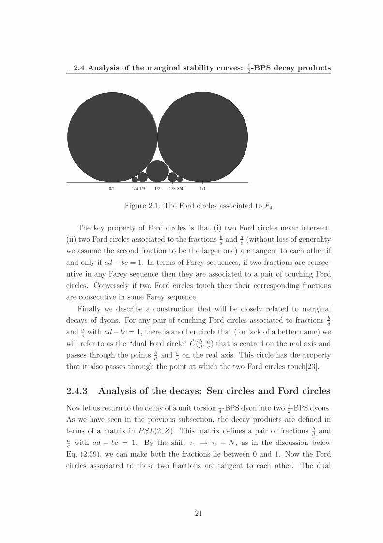
1/20/1 1/11/4 2/3 3/41/3
Figure 2.1: The Ford circles associated to F4
The key property of Ford circles is that (i) two Ford circles never intersect,
(ii) two Ford circles associated to the fractions bd
and ac
(without loss of generality
we assume the second fraction to be the larger one) are tangent to each other if
and only if ad − bc = 1. In terms of Farey sequences, if two fractions are consec-
utive in any Farey sequence then they are associated to a pair of touching Ford
circles. Conversely if two Ford circles touch then their corresponding fractions
are consecutive in some Farey sequence.
Finally we describe a construction that will be closely related to marginal
decays of dyons. For any pair of touching Ford circles associated to fractions bd
and ac
with ad− bc = 1, there is another circle that (for lack of a better name) we
will refer to as the “dual Ford circle” C( bd, a
c) that is centred on the real axis and
passes through the points bd
and ac
on the real axis. This circle has the property
that it also passes through the point at which the two Ford circles touch[23].
2.4.3 Analysis of the decays: Sen circles and Ford circles
Now let us return to the decay of a unit torsion 14-BPS dyon into two 1
2-BPS dyons.
As we have seen in the previous subsection, the decay products are defined in
terms of a matrix in PSL(2, Z). This matrix defines a pair of fractions bd
andac
with ad − bc = 1. By the shift τ1 → τ1 + N , as in the discussion below
Eq. (2.39), we can make both the fractions lie between 0 and 1. Now the Ford
circles associated to these two fractions are tangent to each other. The dual
21

2.4 Analysis of the marginal stability curves: 12-BPS decay products
Ford circle C(
bd, a
c
)has its origin on the real axis at the midpoint of these two
fractions, at ad+bc2cd
. Its radius is given by half the distance between these two
fractions, namely 12cd
. Thus the equation of this dual Ford circle is:
(τ1 −
ad + bc
2cd
)2
+ τ 22 =
1
4c2d2(2.46)
Comparing with Eq. (2.37), we see that the dual Ford circle is the limit of the Sen
circle for marginal decays of a unit torsion 14-BPS dyon into two 1
2-BPS dyons, as
E → 0. (Recall that E was defined in Eq. (2.38)). Conversely, the Sen circle can
be thought of as a deformation of the dual Ford circle with deformation parameter
E. For given integers a, b, c, d, both circles are centred at the same value of τ1
but have their centres vertically displaced from each other. The radius of the Sen
circle is such that it intersects the real axis in the same pair of points as the dual
Ford circle. Note that E
cdcan be positive or negative, so the Sen circle can be
displaced either downwards or upwards relative to the dual Ford circle.
This similarity is intriguing and may point to a more profound relation be-
tween Sen circles and Ford circles that we have not yet uncovered (in particular,
it seems plausible that by deforming the K3 moduli one can set E → 0, which
would make the two circles actually coincide). However, already the relation we
have exhibited is sufficient to understand a key property of Sen circles, which is
that they do not intersect in the upper half plane, but only on the real axis[10].
This can can be seen as follows. Every Sen circle is associated to a dual
Ford circle and thereby to a pair of Ford circles. Consider the two Sen circles
associated to a, b, c, d and h, p, k, q with ad − bc = pk − qh = 1. Clearly we havebd
< ac
as well as hk
< p
q. The two possible orderings of the fractions are b
d, h
k, a
c, p
q
and bd, a
c, h
k, p
q. The first ordering is ruled out by the Ford circle construction, since
it implies that the Ford circle of the first fraction touches that of the third one,
while the Ford circle of the second fraction touches that of the fourth one. This
contradicts the fact that all the Ford circles are non-overlapping. Thus only the
second ordering is possible, where we have the fractions bd, a
c, h
k, p
qin increasing
order. Let us consider the case where ac
= hk, so that the Sen circles touch on the
real axis. Clearly the dual Ford circles also touch on the real axis, which means
the three fractions bd, a
c, p
qare consecutive terms in a Farey sequence.
22

2.4 Analysis of the marginal stability curves: 12-BPS decay products
We want to show that the Sen circles in this case do not intersect in the upper
half plane. This imposes a condition on the slopes of the Sen circles at the real
axis. From Eq. (2.37) we find that the slope at the real axis is given by:
tanφ = ± 1
E(2.47)
where the two signs hold for the two intersection points. Now it is easy to check
that the condition we are seeking is:
E(a, b, c, d) + E(a, p, c, q) > 0 (2.48)
This is of course satisfied if both E’s are positive, though that is not in general
the case. But even in the general case the condition above does hold, as we now
demonstrate. From the definition of E one finds that:
E(a, b, c, d)+E(a, p, c, q) =1√∆
(c(q+d)Q2+a(p+b)P 2−(a(q + d) + c(p + b)) P ·Q
)
(2.49)
Now we use the fact, explained in the discussion around Eq. (2.45), that if three
fractions are consecutive in a Farey sequence then the middle one is the mediant
of the other two. Hence we have:
a
c=
p + b
q + d(2.50)
from which we get:
Na = (p + b), Nc = (q + d) (2.51)
for some integer N ≥ 1. It follows that:
E(a, b, c, d) + E(a, p, c, q) =N√∆
(c ~Q − a~P )2 > 0 (2.52)
as desired. By similar methods the non-intersecting property of Sen circles can
be proved for the case where bd, a
c, h
k, p
qare all distinct fractions.
2.4.4 Analysis of the decays: higher torsion case
The above discussion was for the case of a unit torsion dyon as the initial state.
Now let us look at the case where the initial state is a dyon with torsion ≥ 2. In
23

2.4 Analysis of the marginal stability curves: 12-BPS decay products
this case the Sen circle is replaced by Eq. (2.41), which intersects the real axis at
the points ac
and mbnd
. Let us now analyze the condition Eq. (2.40) in some detail.
Because m and n are co-prime, writing this condition as adn = m(bc+n) tells us
that m divides ad and also that n divides bc. Therefore we can rewrite Eq. (2.40)
as:ad
m− bc
n= 1 (2.53)
where each of the terms on the LHS is an integer. This can only be realized if,
for some (not necessarily prime or unique) factorization of m and n;
m = pq, n = kl (2.54)
we have that:
a′ =a
p, b′ =
b
k, c′ =
c
l, d′ =
d
q(2.55)
are all integers. Evidently they satisfy a′d′ − b′c′ = 1. Substituting in the curve
of marginal stability for this case, Eq. (2.41), we find:
(τ1 −
p
l
a′d′ + b′c′
2c′d′
)2
+
(τ2 +
p
l
E′
2c′d′
)2
=p2
4l2c′2d′2(1 + E′2) (2.56)
where
E′ ≡ mn√∆
(q
kc′d′ Q2 +
k
qa′b′ P 2 − (a′d′ + b′c′)Q · P
)(2.57)
This curve intersects the real axis at the points:
p
l
b′
d′ ,p
l
a′
c′, (2.58)
For a fixed value of p
l, the set of intersection points is in one to one correspondence
with those for the unit torsion case, where using Ford circles (or the methods of
Ref.[10]) we saw that curves of marginal stability do not intersect. However the
value of p
lis not fixed. For given m, n specifying a higher torsion dyon, Eq. (2.54)
permits several solutions for p and l in general. For each of them we obtain a
construction in 1-1 correspondence with the set of curves of marginal stability for
the unit torsion case, and it appears quite likely that curves from one of these
sets can intersect with curves from another set. This would result in curves of
marginal stability that intersect each other in the upper half plane.
24

2.4 Analysis of the marginal stability curves: 12-BPS decay products
To generate examples, it is convenient to revert to the notation in which the
charges of the decay products are labelled by a matrix of integers
(m1 r1
s1 n1
)
satisfying Eqs.(2.32) and (2.33). From these two equations we find that:
m1n + n1m = mn (2.59)
from which we see that m1 is a multiple of m. We write:
m1 = mα1 (2.60)
where α1 is another integer. The equations now yield the following general form
for the matrix: (m1 r1
s1 n1
)=
(mα1
mn α1(1−α1)s1
s1 n(1 − α1)
)(2.61)
The strategy is now to choose a value for α1 and then look for the set of s1 that
divide mn α1(1 − α1). Finally to ensure that we are dealing with a two-body
decay, we must check that there is no overall common factor in either of the
matrices (m1 r1
s1 n1
),
(m − m1 −r1
−s1 n − n1
)(2.62)
In this way we can generate a large number of examples of curves of marginal
stability for higher torsion dyons decaying into a pair of 12-BPS dyons.
To check the possible intersections of such curves, we recall that they intersect
the real axis in the points m1−ms1
and m1
s1. If two such intervals intersect then the
curves will necessarily intersect in the upper half-plane. Let us consider a definite
example. Suppose (m, n) = (2, 3). Then choosing α1 = 1, we see that s1 can be
arbitrary. On the other hand choosing α1 = 2 we find that the allowed values
of s1 are 1, 2, 3, 4, 6, 12. It is easy to check that for the very simplest choices the
curves do not intersect. However, picking α1 = 1, s1 = 7 and α1 = 2, s1 = 12 we
find that all the conditions are satisfied and the decay products are given by the
matrices:
α1 = 1, s1 = 7 :
(2 0
7 0
),
(0 0
−7 3
)
α1 = 2, s1 = 12 :
(4 −1
12 −3
),
(−2 1
−12 6
)(2.63)
25

2.5 Analysis of the marginal stability curves: 14-BPS decay products
In terms of the integers a, b, c, d the two decay processes are parametrised by the
matrices:
(i)
(a b
c d
)=
(2 0
7 1
)
(ii)
(a b
c d
)=
(1 1
3 4
)(2.64)
Each matrix satisfies 3ad − 2bc = 6.
Now the curves of marginal stability for the two decay modes intersect the
real axis at the following values:
(i) τ1 = 0,2
7
(ii) τ1 =1
6,
1
3(2.65)
These two intervals are overlapping, hence the associated curves must intersect in
the interior of the upper half plane. We conclude that curves of marginal stability
for the decay of higher torsion dyons can in general intersect in the upper half
plane, unlike what happens for unit torsion dyons. It would be important to
understand the physical and mathematical reasons why the curves intersect, as
well as the consequences of this fact.
2.5 Analysis of the marginal stability curves: 14-
BPS decay products
2.5.1 Decays into a 12-BPS and a 1
4-BPS dyon
We now consider decays of a 14-BPS dyon into one 1
2-BPS and one 1
4-BPS dyon.
This is parametrised as in Eq. (2.14). If the first decay product is taken to be 12-
BPS then we must impose the condition Eq. (2.32) which is solved by Eq. (2.34).
However, the coefficients mi, ri, si, ni are no longer required to be integers and
therefore nor are a, b, c, d. Moreover we want the second state to be 14-BPS and
therefore adn − bcm 6= mn. Finally, as indicated earlier, we must check that
26

2.5 Analysis of the marginal stability curves: 14-BPS decay products
the curve we obtain from Eq. (2.21) actually describes the forward and not the
reverse decay process.
Consider the case where the initial state is a unit torsion dyon with (m, n) =
(1, 1). For this case we find the curve of marginal stability to be:
(τ1 −
m1 − n1
2s1
)2
+
(τ2 +
E
2s1
)2
=1
4s21
((m1 − n1)
2 + 4r1s1 + E2)
(2.66)
where
E ≡ 1√∆
(s1 Q2
R − r1 P 2R − (m1 − n1)QR · PR
)(2.67)
On replacing m1, r1, s1, n1 by their expressions in terms of a, b, c, d we can also
bring it to the form:
(τ1 −
ad + bc
2cd
)2
+
(τ2 +
E
2cd
)2
=1
4c2d2
((ad − bc)2 + E2
)(2.68)
with
E ≡ 1√∆
(cd Q2
R + ab P 2R − (ad + bc)QR · PR
)(2.69)
The equation is very similar to the Sen circle for decays of a unit torsion dyon into12-BPS decay products. However, the constraints on a, b, c, d are quite different.
Instead of analyzing this case further, we will return to it as a special case of the
more general decay into two 14-BPS states.
2.5.2 Decays into two 14-BPS dyons
We now address the case in which the initial 14-BPS dyon decays into a pair of
14-BPS dyons. Again we start with the unit torsion case, (m, n) = (1, 1). The
relevant curve of marginal stability is the same as in the previous subsection,
Eq. (2.66), except that the determinants of
(mi ri
si ni
)are both nonzero. (Later
we will also be able to specialize to the case where one of them is zero.)
Let us now address the constraints on the final state parameters that are
required to ensure that the decay process corresponds to the correct branch of
Eq. (2.18). First of all, the quantity ∆ that appears in the BPS mass formula
27

2.5 Analysis of the marginal stability curves: 14-BPS decay products
Eq. (2.10) involves a square root, and we have taken all square roots to be positive.
This has the following consequence. Observe that:
∆(mi~Q + ri
~P , si~Q + ni
~P ) = det
(mi ri
si ni
)∆( ~Q, ~P ) (2.70)
Positivity of ∆ on both sides of the equation imposes the condition:
det
(mi ri
si ni
)> 0, i = 1, 2 (2.71)
Since (m2 r2
s2 n2
)=
(1 − m1 −r1
−s1 1 − n1
)(2.72)
we find that:
m1n1 − r1s1 > max (m1 + n1 − 1, 0) (2.73)
For what follows, it will be convenient to introduce the eigenvalues β1, γ1 of(m1 r1
s1 n1
)and β2, γ2 of
(m2 r2
s2 n2
). Because the two matrices commute (they
are of the form F and 1−F) they can be simultaneously diagonalised, from which
we see that:
β1 + β2 = 1 = γ1 + γ2 (2.74)
From the determinant conditions above, we have:
β1γ1 > 0, (1 − β1)(1 − γ1) > 0 (2.75)
We will now examine the quantities M1
M, M2
Mon the curve Eq. (2.66). For
convenience, we would like to choose a particular point on the curve and evaluate
these quantities there. The possible results are as follows. If we find M1
M> 1 at a
point, then the marginal stability curve cannot correspond to M = M1 + M2. It
may correspond to either M1 = M +M2 or M2 = M +M1. Which of the two cases
it corresponds to is then not very important, but can be distinguished by looking
at M2
M. If on the other hand we find M1
M< 1 then we have the possibilities of being
on the correct branch M = M1 +M2 or on the wrong branch M2 = M +M1. This
time it is essential to distinguish the two, which can again be done by evaluatingM2
M. Being on the correct branch requires Mi
M< 1 for both i = 1 and 2.
28
2.5 Analysis of the marginal stability curves: 14-BPS decay products
In any of these cases, having determined the relevant branch of Eq. (2.18) at
one point on the curve, we can be sure that we will not cross over to another
branch elsewhere on the same curve, since crossing from one branch to another
requires passing through a point where one of the masses vanishes. But the BPS
mass formula does not vanish for any value of the moduli, so this is not possible
(unless the charges of that state vanish identically).
Let us assume that the matrix
(m1 r1
s1 n1
)is such that the curve Eq. (2.66)
intersects the real axis. This will happen if the eigenvalues β1, γ1 are both real
(without loss of generality we take γ1 ≥ β1). Then, a convenient point at which
to evaluate the mass ratios is one of the intersection points of the curve with the
real axis. Setting τ2 = 0 in Eq. (2.21), we get the following equation for τ1:
n1 −r1
τ1
= m1 − τ1s1 (2.76)
Now let us consider the expressionM2
1
M2 in the limit τ2 → 0. We have:
M21
M2
∣∣∣∣τ2→0
=[(m1
~QR + r1~PR) − τ1(s1
~QR + n1~PR)]2
[ ~QR − τ1~PR]2
=[(m1 − τ1s1) ~QR − τ1(n1 − r1
τ1)~PR]2
[ ~QR − τ1~PR]2
(2.77)
Using Eq. (2.76) we now get:
M1
M
∣∣∣∣τ2→0
= |m1 − τ1s1| (2.78)
On the real axis, Eq. (2.66) gives:
τ1 =1
2s1
(± (γ1 − β1)| + (m1 − n1)
)(2.79)
Inserting this into Eq. (2.78) we find:
m1 − τ1s1 = β1 or γ1 (2.80)
Let us first consider the case m1n1−r1s1 > 1. We will show that in this region
the decay is not the desired one, but corresponds instead to a branch of Eq. (2.18)
29
2.5 Analysis of the marginal stability curves: 14-BPS decay products
describing a reverse decay. With this condition on the determinant, one of the
eigenvalues (say γ1) must be > 1. Positivity of the second determinant, which
equals (1 − β1)(1 − γ1), tells us that if γ1 > 1 then also β1 > 1. Thus we have
that both eigenvalues are > 1. It follows that M1
M> 1 and we are, as promised,
on the wrong branch.
Next suppose m1n1 − r1s1 = 1. The above considerations then show that
β1 = γ1 = 1. Then we M1
M= 1. This means M2 = 0 and therefore the charges
associated to the second state are identically zero. In other words,
(m1 r1
s1 n1
)=
(0 0
0 0
). This is a trivial case where the first decay product is the original state
itself.
Let us note at this point that if m1, r1, s1, n1 had been taken to be integers,
and the corresponding state was restricted not to be 12-BPS, we would necessarily
have m1n1 − r1s1 ≥ 1. We have shown that all such cases do not correspond to
a valid decay of M into M1 and M2, therefore no such decays exist for integer
coefficients. This is one of the key results of Ref.[15].
That leaves the case
0 < m1n1 − r1s1 < 1, 0 < m2n2 − r2s2 < 1 (2.81)
which can only be satisfied for fractional coefficients.
Requiring β1γ1 < 1 and also β2γ2 = (1 − β1)(1 − γ1) < 1 we see that 0 <
β1, γ1 < 1 and 0 < β2, γ2 < 1. From this and Eq. (2.80) we find M1
M< 1, M2
M<
1 and this indeed corresponds to the decay process that we were looking for.
Thus Eq. (2.81) provides a necessary condition for the coefficients m1, n1, r1, s1
in Eq. (2.14) in order to have a decay of the original dyon into two 14-BPS dyons.
Under this condition, our curve Eq. (2.21) describes the marginal stability locus
in the τ1, τ2 plane. However this is a locus of co-dimension 2 or more in the
full moduli space, for the following reason. Fractional m1, r1, s1, n1 means that
the decay process in terms of the original integral charge vectors was into states
living outside the ~Q, ~P plane. This is precisely the case, referred to earlier, where
the moduli in M need to be adjusted to make the final state charges (after R
projection) lie in the same plane as the initial state charges[15]. We will explore
30

2.6 Discussion
the sufficient conditions on the values of m1, r1, s1, n1 as well as to understand
more precisely the condition on the moduli matrix M which put the projected
charge vectors in the plane of the decaying dyon.
2.6 Discussion
We have found a general equation for marginal stability of 14-BPS dyons to de-
cay into two final state particles, Eq. (2.21). Analysis of the equation reveals
many distinct cases with different properties. We will extend this analysis to
multi-particle final states in next chapter. The construction of Ford circles and
especially their dual circles proved useful in this analysis and we suspect that
there may be a deeper mathematical relationship to the Sen circles of marginal
instability for unit torsion dyons decaying into 12-BPS final states.
31

Chapter 3
Constraints on “rare” dyon
decays
After deriving the curve of marginal stability in terms of constraint equation on
the torus modular parameter, now we obtain the complete set of constraints on all
the moduli of N = 4 superstring compactifications that permit “rare” marginal
decays of 14-BPS dyons to take place. The constraints are analyzed in some special
cases. The analysis extends in a straightforward way to multi-particle decays. We
will then discuss the possible relation between general multi-particle decays and
multi-centred black holes.
3.1 Introduction
In the previous chapter we have analyzed in detail the lines of marginal stability
corresponding to decays of 14BPS states into 2 1
2BPS states. We also saw that
there are many more types of marginal decays in the theory, and in one sense
they are far more generic. These decays are into a pair of 14-BPS final states, or
into three or more final states each of which can be 12-BPS or 1
4-BPS. In another
sense these decays are “rare”, which we also discussed in details in the earlier
chapter of this thesis, (at least for unit-torsion initial dyons) that they take place
on curves of marginal stability that have a co-dimension > 1 in the moduli space1.
1Therefore they should not technically be called “curves”, but we use this terminology
anyway and hope it does not cause confusion.
32

3.1 Introduction
Therefore these have been labelled “rare decays”. In particular they cannot lead
to jumps in the degeneracy formula1. Nevertheless the existence of such decay
modes is of importance in understanding the behavior of dyons as we move around
in moduli space, and we will study them here for their own sake as well as for
possible interesting physical consequences that they may turn out to have.
In previous chapter these curves were precisely characterized as circles in the
upper half-plane labelled by the parameter τ corresponding to the SL(2)/U(1)
factor of the moduli space2. These circles depend on the other moduli as well.
However, as was demonstrated in Refs.[15, 26, 27], there are additional conditions
that need to be imposed on the remaining moduli in order to make the decay
possible. These latter conditions have not yet been worked out. In this chapter we
will obtain these conditions and thereby completely characterize the codimension
> 1 subspace on which rare decays can take place.
It is also known that there exist multi-centred dyonic black holes with two 14-
BPS centres, or three or more centres each of which can be 12- or 1
4-BPS. However,
because the degeneracy formula does not jump at curves of marginal stability,
these multi-centred dyons have not played a role in studies of dyons in N = 4
compactifications. In particular they have not been related to marginal decays
into two 14-BPS final states or multiple final states, and in fact such a relation
does not seem necessary for the state-counting problem. Nevertheless, in what
follows we will argue that the relation between curves of marginal stability and
multi-centred black holes flying apart is quite generic.
In what follows, we start by briefly reviewing the “rare” marginal decays in
N = 4 compactifications. Then we find a precise form for the constraints on
moduli space in order for such rare decays to take place. We examine and solve
these constraints in a variety of special cases, to give a flavour of what they look
like. Then using some known results on T-duality orbits, we will obtain the con-
straints in the general case. Next we recursively identify the loci of marginal
1For higher-torsion initial dyons the curves can be of codimension 1, but the degeneracy
(or rather, index) is still not expected to jump, because of fermion zero modes. We will focus
largely on unit-torsion dyons in this paper.2In the type IIB on K3×T
2 description this τ is the modular parameter of the geometrical
torus, hence we sometimes refer to the τ UHP as the “torus moduli space” – although technically
it would be more accurate to call it the Teichmuller space of the torus.
33

3.2 Marginal stability for N = 4 dyons
stability for multi-particle decays. Finally we examine the special-geometry for-
mula for generic multi-centred black holes and write it in a form that relates their
separations to curves of marginal stability for n ≥ 2-body decays.
3.2 Marginal stability for N = 4 dyons
The electric and magnetic charge vectors of a dyon in an N = 4 string compactifi-
cation are elements of a 28 dimensional integral charge lattice of signature (6, 22).
The formulae for BPS mass involve a 28 × 28 matrix L, which in our basis will
be taken to be:
0 II6 0
II6 0 0
0 0 −II16
(3.1)
as well as a 28 × 28 matrix M of moduli satisfying MLMT = L. The inner
product of charge vectors appearing in the BPS mass is taken with the matrix
L+M . In the heterotic basis where the compactification is specified by a constant
metric Gij, an antisymmetric tensor field Bij and constant gauge potentials AIi
(where i = 1, 2, · · · , 6 and I = 1, 2, · · · , 16), this matrix is [28, 29]:
L+M =
G−1 1 + G−1(B + C) G−1A
1 + (−B + C)G−1 (G − B + C)G−1(G + B + C) (G − B + C)G−1A
AT G−1 AT G−1(G + B + C) AT G−1A
(3.2)
Here C is a symmetric 6 × 6 matrix constructed from A as C = 12AT A, more
concretely Cij = 12AI
i AIj .
In this basis we parametrise the charge vectors explicitly as:
~Q =
~Q′(6)
~Q′′(6)
~Q′′′(16)
, ~P =
~P ′(6)
~P ′′(6)
~P ′′′(16)
(3.3)
where we have broken up the original vectors into three parts with 6,6 and 16
components respectively. In subsequent discussions we will not explicitly write
out the subscripts (6), (16) that appear in the above formula.
34

3.2 Marginal stability for N = 4 dyons
The BPS mass formula for 14-BPS dyons in N = 4 compactifications was
defined in Eq. (2.10). The inner products of charge vectors appearing in mass
formula are of the form:
Q P ≡ ~QT (L + M)~P (3.4)
The matrix L + M has 22 zero eigenvalues and therefore the inner product only
contains a projected set of 6 components from the original 28 components of the
charge vector. Explicitly, the zero eigenvectors take the form:
G + B + C AI
−1 0
0 −1
(3.5)
where each column of the above matrix describes an independent zero eigenvector.
It is convenient to replace the inner product on charge vectors in Eq. (3.4)
by an ordinary product acting on some projected vectors. To do this, define√L + M as a 28 × 28 matrix satisfying
√L + M
T√L + M = L + M . This will
be ambiguous upto a “gauge” freedom but we will select a specific solution that
is particularly useful, namely:
√L + M =
E−1 E−1(G + B + C) E−1A
0 0 0
0 0 0
(3.6)
where E stands for the vielbein: Eai Ea
i = Gij.
With this matrix it is evident that the projected charges only have their first 6
components nonzero, namely for any arbitrary vectors ~Q, ~P the projected vectors~QR, ~PR defined by:
~QR =√
L + M ~Q, ~PR =√
L + M ~P (3.7)
are 6-component vectors. The components of these vectors are moduli dependent
and not quantized. On the projected vectors, one only needs to consider ordinary
inner products, for example ~QTR
~QR is equal (by construction) to ~QT (L + M) ~Q.
Hence in what follows we will denote this quantity either by ~Q ~Q or equivalently
by ~QR · ~QR, and analogously for other inner products.
35

3.2 Marginal stability for N = 4 dyons
Within the 6-dimensional projected charge space, the electric and magnetic
charge vectors of the initial dyon span a 2-dimensional plane. Decay of a 14-BPS
dyon into a set of decay products with quantized charge vectors ( ~Q(1), ~P (1)), · · · , ( ~Q(n), ~P (n))
can take place only when the plane spanned by the projected charge vectors of
each decay product coincides with this plane (this is the condition for all states
to be mutually 14-BPS):
(~Q
(i)R
~P(i)R
)=
(mi ri
si ni
)(~QR
~PR
)(3.8)
When there are just two decay products and both are 12-BPS, the pair of decay
products defines a 2-plane. Charge conservation then implies that this plane
coincides with the plane of the original charge vectors, so in this very special
case the above requirement imposes no conditions on the moduli. Indeed, the
numbers mi, ri, si, ni are then integers and the above relation holds between the
full (quantized) charge vectors, not only the projected ones. Marginal decay
takes place on a wall of marginal stability whose equation is explicitly known
(see Ref.[10] and references therein). In all other cases, the numbers mi, ri, si, ni
are non-integral and moduli-dependent. In these cases the above condition puts
additional constraints on the background moduli M . Our goal here is to identify
these constraints explicitly.
For a two-body decay into 14-BPS constituents, once the constraints are satis-
fied and we find the numbers m1, r1, s1, n1 (the corresponding numbers m2, r2, s2, n2
are determined by charge conservation) the condition for marginal decay is ex-
pressed in terms of the curve [26] Eq. (2.21). We rewrite the curve for the case
of unit torsion in following form:
(τ1 −
m1 − n1
2s1
)2
+
(τ2 +
E
2s1
)2
=1
4s21
((m1 − n1)
2 + 4r1s1 + E2)
(3.9)
Here we have restricted to the case of unit-torsion dyons, so we have put m =
n = 1 with respect to the notation in Ref.[26]. Also, E is defined by:
E ≡ 1√∆
(~Q(1) ~P − ~P (1) ~Q
)(3.10)
36

3.3 Rare dyon decays
We notice that exchanging the role of the two final-state dyons sends E → −E.
It also sends m1 −n1 → (1−m1)− (1−n1) = −(m1 −n1) and r1, s1 → −r1,−s1.
The curve of marginal stability is invariant under this set of transformations, as
it should be.
We now turn to the detailed study general two-body decays into 14-BPS con-
stituents. We will find explicit expressions for the numbers m1, r1, s1, n1 in terms
of the quantized charge vectors ~Q, ~P , ~Q1, ~P1 and the moduli M . We will also ex-
plicitly characterize the loci in moduli space where such rare decays are allowed.
3.3 Rare dyon decays
3.3.1 Analysis and implicit solution
It will be useful to define a quartic scalar invariant of four different vectors by:
∆( ~A, ~B; ~C, ~D) ≡ det
(~A ~C ~A ~D
~B ~C ~B ~D
)= ( ~A ~C)( ~B ~D) − ( ~A ~D)( ~B ~C)
(3.11)
As explained above, the “” product is the moduli-dependent inner product in-
volving the matrix L + M . The above quantity is antisymmetric under exchange
of the first pair or last pair of vectors, and symmetric under exchange of the two
pairs. The quartic invariant of two variables defined earlier is a special case of
this new invariant:
∆( ~Q, ~P ) = ∆( ~Q, ~P ; ~Q, ~P ) (3.12)
Now start with the following vector equation that is part of Eq. (3.8):
~Q(1)R = m1
~QR + r1~PR (3.13)
Contracting this successively with ~QR and ~PR we find:
~Q(1)R · ~QR = m1
~Q2R + r1
~QR · ~PR
~Q(1)R · ~PR = m1
~QR · ~PR + r1~P 2
R (3.14)
Multiplying the first equation by ~P 2R and the second by ~QR · ~PR and subtracting,
we find:
m1∆( ~QR, ~PR) = ∆( ~QR, ~PR; ~Q(1)R , ~PR) (3.15)
37

3.3 Rare dyon decays
which enables us to solve for m1. Repeating this process we can solve for r1, s1, n1
leading to the result:(
m1 r1
s1 n1
)=
1
∆( ~QR, ~PR)
(∆( ~QR, ~PR; ~Q
(1)R , ~PR) ∆( ~QR, ~PR; ~QR, ~Q
(1)R )
∆( ~QR, ~PR; ~P(1)R , ~PR) ∆( ~QR, ~PR; ~QR, ~P
(1)R )
)
(3.16)
It follows that Eq. (3.8) can be expressed as:(
~Q(1)R
~P(1)R
)=
1
∆( ~QR, ~PR)
(∆( ~QR, ~PR; ~Q
(1)R , ~PR) ∆( ~QR, ~PR; ~QR, ~Q
(1)R )
∆( ~QR, ~PR; ~P(1)R , ~PR) ∆( ~QR, ~PR; ~QR, ~P
(1)R )
)(~QR
~PR
)
(3.17)
For fixed, quantized charge vectors ~Q, ~P of the initial dyon and ~Q(1), ~P (1) of the
first decay product (the charge of the second product is determined by charge
conservation), the above equation provides a set of constraints on the moduli
that must be satisfied for the 14→ 1
4+ 1
4decay to be possible. These constraints
together with the curve of marginal stability Eq. (2.21) provide a necessary and
sufficient set of kinematic conditions for marginal decay.
In the above form, it is rather difficult to disentangle the constraints or to
physically understand their significance. Therefore we will consider a number
of special cases. Along the way we will see the advantage of using T-duality
to bring the charges into a convenient form and performing the analysis in that
basis. Finally we write down the explicit constraint equation in the general case,
again in the chosen T-duality basis.
3.3.2 Explicit solution: special cases
(i) 12-BPS final states
The case where the decay products are 12-BPS should provide no constraints on
the moduli as this is a “non-rare” decay. This provides a check on our equations.
Inserting the 12-BPS conditions:
~P (1) =k1
l1~Q(1), ~P (2) =
k2
l2~Q(2) (3.18)
with ki, li integers, we find that:(
m1 r1
s1 n1
)=
(k2
l2− k1
l1
)∆( ~Q
(1)R , ~Q
(2)R )
∆( ~QR, ~PR)
(k2
l2−1
k1k2
l1l2−k1
l1
)(3.19)
38

3.3 Rare dyon decays
We also have:
∆( ~QR, ~PR) =
(k2
l2− k1
l1
)2
∆( ~Q(1)R , ~Q
(2)R ) (3.20)
Substituting in the above equation, we find:
(m1 r1
s1 n1
)=
1
k2l1 − k1l2
(k2l1 −l1l2
k1k2 −k1l2
)(3.21)
At this stage all moduli-dependence has disappeared from the matrix, and equa-
tion Eq. (3.8) indeed provides no constraints on the moduli. Rather, it reduces to
an identity. It is also easy to see that k1l2−k2l1 divides the torsion of the original
dyon, so if we are also considering the unit-torsion case then k1l2 − k2l1 = 1 and
m1, r1, s1, n1 are all manifestly integral [10].
(ii) Special charges and moduli
The next special case we will study has a restricted set of charges. Additionally,
some of the background moduli are set to a specific value, namely zero in the
chosen coordinates. We then examine the constraints on the remaining mod-
uli. In choosing special values for the moduli, we should in principle avoid loci
of enhanced gauge symmetry where the dyons we are studying would become
massless.
Let us restrict ourselves to special initial-state charges given by:
~Q′ = (Q′1, 0, · · · , 0), ~Q′′ = (Q′′
1, 0, · · · , 0), ~Q′′′ = 0 (3.22)
and
~P ′ = (0, P ′2, 0, · · · , 0), ~P ′′ = (0, P ′′
2 , 0, · · · , 0), ~P ′′′ = 0 (3.23)
Next we set Bij = 0 = AIi as well as Gij = 0, i 6= j. The above restrictions
allow us to choose the orthonormal frames Eai to be diagonal:
Eii = Ri, i = 1, 2, · · · , 6 (3.24)
with Ri the radii of the six compactified directions in the heterotic basis.
39

3.3 Rare dyon decays
In the restricted subspace of moduli space that we are considering here, the
matrix√
L + M reduces to:
√L + M =
E−1 E 0
0 0 0
0 0 0
(3.25)
with E given as in Eq. (3.24). Therefore the projected initial-state charge vectors
are:
~QR =
Q′
1
R1+ Q′′
1R1
0
...
0
, ~PR =
0P ′
2
R2+ P ′′
2 R2
0
...
0
(3.26)
For this configuration we clearly have ~QR · ~PR = 0 and therefore the quartic
invariant ∆ is:
∆(QR, PR) =
(Q′
1
R1
+ Q′′1R1
)2(P ′
2
R2
+ P ′′2 R2
)2
(3.27)
We take the decay products to have generic charges ~Q(1), ~P (1) and ~Q(2), ~P (2)
subject of course to the requirement that they add up to ~Q, ~P . We then have:
~Q(1)R =
Q(1)′
1
R1+ Q
(1)′′
1 R1
Q(1)′
2
R2+ Q
(1)′′
2 R2
...
Q(1)′
6
R6+ Q
(1)′′
6 R6
, ~P(1)R =
P(1)′
1
R1+ P
(1)′′
1 R1
P(1)′
2
R2+ P
(1)′′
2 R2
...
P(1)′
6
R6+ P
(1)′′
6 R6
(3.28)
40
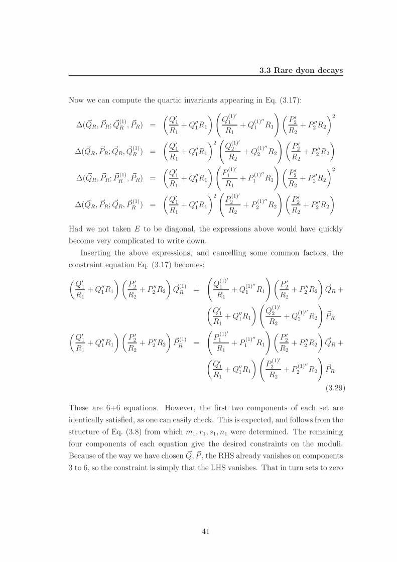
3.3 Rare dyon decays
Now we can compute the quartic invariants appearing in Eq. (3.17):
∆( ~QR, ~PR; ~Q(1)R , ~PR) =
(Q′
1
R1+ Q′′
1R1
)(Q
(1)′
1
R1+ Q
(1)′′
1 R1
)(P ′
2
R2+ P ′′
2 R2
)2
∆( ~QR, ~PR; ~QR, ~Q(1)R ) =
(Q′
1
R1+ Q′′
1R1
)2(
Q(1)′
2
R2+ Q
(1)′′
2 R2
)(P ′
2
R2+ P ′′
2 R2
)
∆( ~QR, ~PR; ~P(1)R , ~PR) =
(Q′
1
R1
+ Q′′1R1
)(P
(1)′
1
R1
+ P(1)′′
1 R1
)(P ′
2
R2
+ P ′′2 R2
)2
∆( ~QR, ~PR; ~QR, ~P(1)R ) =
(Q′
1
R1
+ Q′′1R1
)2(
P(1)′
2
R2
+ P(1)′′
2 R2
)(P ′
2
R2
+ P ′′2 R2
)
Had we not taken E to be diagonal, the expressions above would have quickly
become very complicated to write down.
Inserting the above expressions, and cancelling some common factors, the
constraint equation Eq. (3.17) becomes:
(Q′
1
R1
+ Q′′1R1
)(P ′
2
R2
+ P ′′2 R2
)~Q
(1)R =
(Q
(1)′
1
R1
+ Q(1)′′
1 R1
)(P ′
2
R2
+ P ′′2 R2
)~QR +
(Q′
1
R1+ Q′′
1R1
)(Q
(1)′
2
R2+ Q
(1)′′
2 R2
)~PR
(Q′
1
R1+ Q′′
1R1
)(P ′
2
R2+ P ′′
2 R2
)~P
(1)R =
(P
(1)′
1
R1+ P
(1)′′
1 R1
)(P ′
2
R2+ P ′′
2 R2
)~QR +
(Q′
1
R1+ Q′′
1R1
)(P
(1)′
2
R2+ P
(1)′′
2 R2
)~PR
(3.29)
These are 6+6 equations. However, the first two components of each set are
identically satisfied, as one can easily check. This is expected, and follows from the
structure of Eq. (3.8) from which m1, r1, s1, n1 were determined. The remaining
four components of each equation give the desired constraints on the moduli.
Because of the way we have chosen ~Q, ~P , the RHS already vanishes on components
3 to 6, so the constraint is simply that the LHS vanishes. That in turn sets to zero
41

3.3 Rare dyon decays
the components 3 to 6 of the vectors ~Q(1)R and ~P
(1)R . Thus we find the constraints:
Q(1)′
i
Ri
+ Q(1)′′
i Ri = 0, i = 3, 4, 5, 6
P(1)′
i
Ri
+ P(1)′′
i Ri = 0, i = 3, 4, 5, 6 (3.30)
If the components of ~Q(1), ~P (1) are all nonvanishing, this implies that:
Ri =
√√√√−Q(1)′
i
Q(1)′′
i
=
√√√√− P(1)′
i
P(1)′′
i
, i = 3, 4, 5, 6 (3.31)
In this special case the constraint equations have some particular features. First
of all, for generic charge vectors ~Q(1) and ~P (1), there are no solutions. To have
any solutions at all, one must choose the charges of the decay products in such
a way that the second equality in the above equation can be satisfied. In other
words, the sign of Q(1)′
i and Q(1)′′
i must be opposite (for i = 3, 4, 5, 6), and the
same has to be true for P (1). In this case we find four constraints on the moduli,
which fix the compactification radii R3, R4, R5, R6.
For this special case, the numbers m1, r1, s1, n1 in Eq. (3.8) are given by:
m1 =Q
(1)′
1R1
+Q(1)′′
1 R1
Q′
1R1
+Q′′
1R1
, r1 =
Q(1)′
2
R2+ Q
(1)′′
2 R2
P ′
2
R2+ P ′′
2 R2
s1 =P
(1)′
1R1
+P(1)′′
1 R1
Q′
1R1
+Q′′
1R1
, n1 =
P(1)′
2
R2+ P
(1)′′
2 R2
P ′
2
R2+ P ′′
2 R2
(3.32)
We see that m1, s1 depend only on R1 and r1, n1 depend only on R2.
So far the decay products were taken to have generic charges (consistent of
course with charge conservation). The situation changes if we choose less generic
decay products. Earlier we took all components of ~Q(1), ~P (1) are nonvanishing.
However if Q(1)′
i = Q(1)′′
i = P(1)′
i = P(1)′′
i = 0 for any i ∈ 3, 4, 5, 6 then the
corresponding constraint Eq. (3.30) is trivially satisfied. In this situation we will
have a reduced number of constraints. As an example if the above situation
holds for all directions except i = 3 and ifQ
(1)′
3
Q(1)′′
3
=P
(1)′
3
P(1)′′
3
then there is only a single
constraint coming from the above equations. The curve of marginal stability
42

3.3 Rare dyon decays
provides one more constraint, so the decay will take place on a codimension-2
subspace of the restricted moduli space in which we are working for this class of
examples. The fact that in some situations there are no solutions (for example if
we do not satisfy that Q(1)′
i and Q(1)′′
i have opposite signs for i = 3, 4, 5, 6) simply
means that our restricted moduli space fails to intersect the marginal stability
locus in that case.
If the charges Q(1)′
i , Q(1)′′
i , P(1)′
i , P(1)′′
i vanish for all i ∈ 3, 4, 5, 6 then there are
no constraints (beyond the curve of marginal stability). This corresponds to two
distinct solutions. One is that the final states are now both 12-BPS. The other
possibility is that they are still 14-BPS, but apparent contradiction of having no
constraints on the moduli is resolved by the fact that we are already in a restricted
subspace of the moduli space.
(iii) General charges, “diagonal” moduli
In this subsection we study rare decays allowing for completely general charges
~Q, ~P , but we will restrict the moduli so that the formulae are tractable. The
situation turns out to be rather similar to the case studied in the previous sub-
section.
Considerable simplification can be brought about in the formulae by using
some known results on T-duality orbits from Ref.[30] (as reviewed in Appendix A
of [31]). For this purpose we first change basis from the L matrix used in Ref.[31]:
L′ =
σ1 0 · · · 0 0 · · · 0
0 σ1 · · · 0 0 · · · 0
0 · · · 0 0 · · · 0
0 · · · 0 σ1 0 · · · 0
0 · · · −LE8 0
0 · · · 0 −LE8
(3.33)
to the one we have defined in Eq. (3.1). Here σ1 is a Pauli matrix, which occurs
6 times in the above, and LE8 is the Cartan matrix of E8.
In fact using T-duality we will be able to restrict to charge vectors that have
the last 16 components vanishing, therefore we can ignore these components and
43
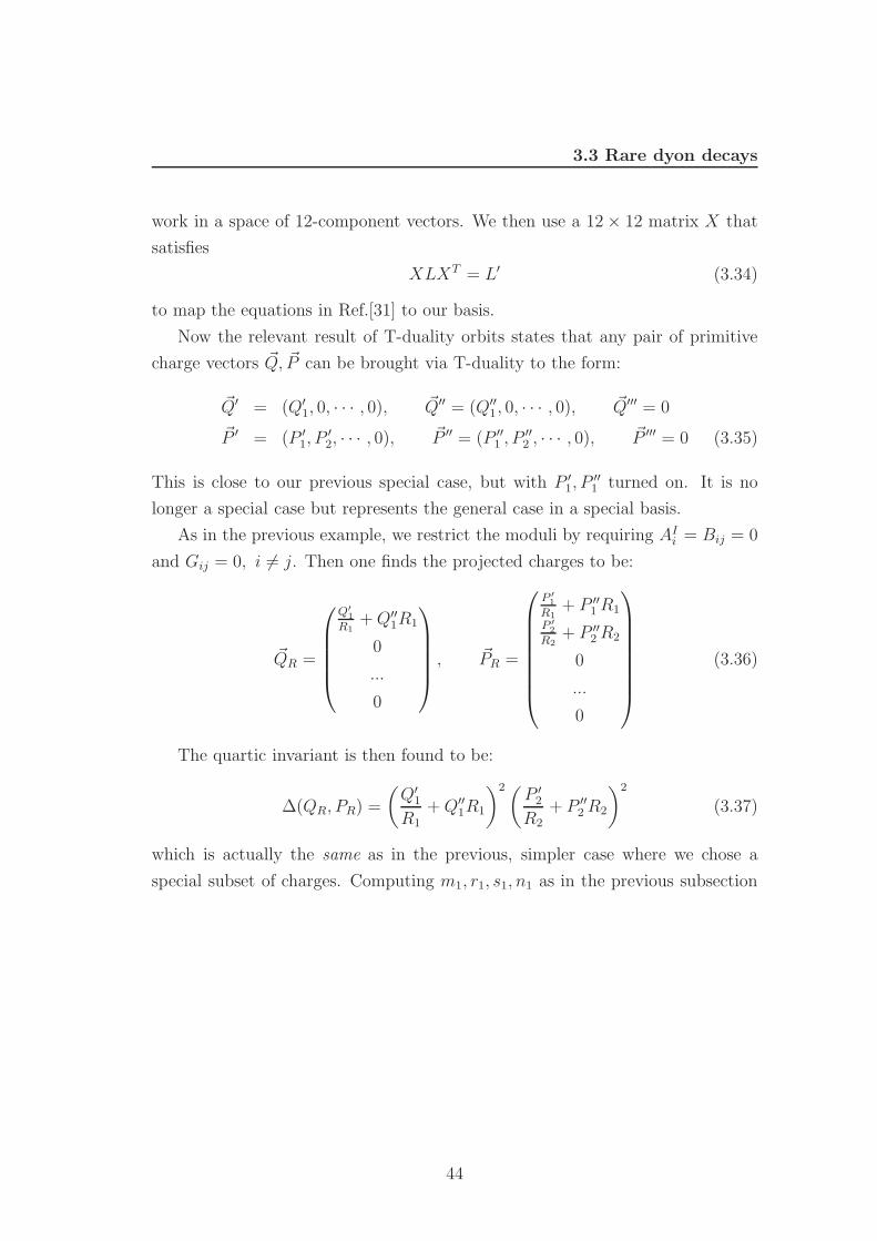
3.3 Rare dyon decays
work in a space of 12-component vectors. We then use a 12 × 12 matrix X that
satisfies
XLXT = L′ (3.34)
to map the equations in Ref.[31] to our basis.
Now the relevant result of T-duality orbits states that any pair of primitive
charge vectors ~Q, ~P can be brought via T-duality to the form:
~Q′ = (Q′1, 0, · · · , 0), ~Q′′ = (Q′′
1, 0, · · · , 0), ~Q′′′ = 0
~P ′ = (P ′1, P
′2, · · · , 0), ~P ′′ = (P ′′
1 , P ′′2 , · · · , 0), ~P ′′′ = 0 (3.35)
This is close to our previous special case, but with P ′1, P
′′1 turned on. It is no
longer a special case but represents the general case in a special basis.
As in the previous example, we restrict the moduli by requiring AIi = Bij = 0
and Gij = 0, i 6= j. Then one finds the projected charges to be:
~QR =
Q′
1
R1+ Q′′
1R1
0
...
0
, ~PR =
P ′
1
R1+ P ′′
1 R1
P ′
2
R2+ P ′′
2 R2
0
...
0
(3.36)
The quartic invariant is then found to be:
∆(QR, PR) =
(Q′
1
R1
+ Q′′1R1
)2(P ′
2
R2
+ P ′′2 R2
)2
(3.37)
which is actually the same as in the previous, simpler case where we chose a
special subset of charges. Computing m1, r1, s1, n1 as in the previous subsection
44

3.3 Rare dyon decays
and inserting them back, the constraint equation can now be written:
(Q′
1
R1+ Q′′
1R1
)(P ′
2
R2+ P ′′
2 R2
)~Q
(1)R =
[(Q
(1)′
1
R1+ Q
(1)′′
1 R1
)(P ′
2
R2+ P ′′
2 R2
)−(
Q(1)′
2
R2+ Q
(1)′′
2 R2
)(P ′
1
R1+ P ′′
1 R1
)]~QR +
(Q′
1
R1+ Q′′
1R1
)(Q
(1)′
2
R2+ Q
(1)′′
2 R2
)~PR
(Q′
1
R1+ Q′′
1R1
)(P ′
2
R2+ P ′′
2 R2
)~P
(1)R =
[(P
(1)′
1
R1
+ P(1)′′
1 R1
)(P ′
2
R2
+ P ′′2 R2
)−(
P(1)′
2
R2
+ P(1)′′
2 R2
)(P ′
1
R1
+ P ′′1 R1
)]~QR +
(Q′
1
R1
+ Q′′1R1
)(P
(1)′
2
R2
+ P(1)′′
2 R2
)~PR
(3.38)
These equations are slightly more complicated than the previous case for which
we had ~Q ~P = 0, but the extra complication is only in the first two components,
which are again trivially satisfied. For the remaining components we find:
Q(1)′
i
Ri
+ Q(1)′′
i Ri = 0, i = 3, 4, 5, 6
P(1)′
i
Ri
+ P(1)′′
i Ri = 0, i = 3, 4, 5, 6 (3.39)
These are exactly the same as the constraints we found in the previous case. The
analysis is therefore also the same: the constraints cannot be satisfied for generic
charges because our restricted moduli space need not intersect the marginal sta-
bility locus. When they can be satisfied there are at most four constraints, though
there will be less if some of the decay product charges vanish.
3.3.3 General charges, “triangular” moduli
In this subsection we restrict the moduli in the most minimal way consistent with
finding a simple form of the constraint equation. The restriction will be a kind
45
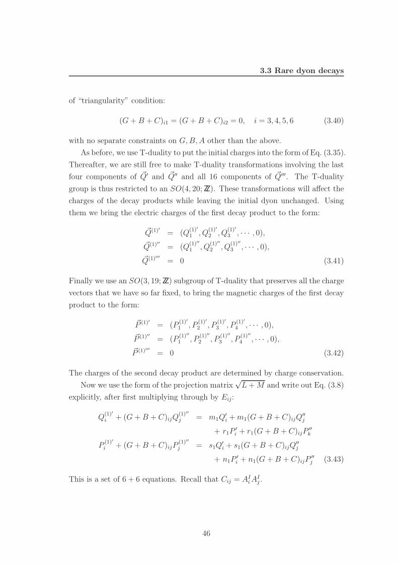
3.3 Rare dyon decays
of “triangularity” condition:
(G + B + C)i1 = (G + B + C)i2 = 0, i = 3, 4, 5, 6 (3.40)
with no separate constraints on G, B, A other than the above.
As before, we use T-duality to put the initial charges into the form of Eq. (3.35).
Thereafter, we are still free to make T-duality transformations involving the last
four components of ~Q′ and ~Q′′ and all 16 components of ~Q′′′. The T-duality
group is thus restricted to an SO(4, 20; ZZ). These transformations will affect the
charges of the decay products while leaving the initial dyon unchanged. Using
them we bring the electric charges of the first decay product to the form:
~Q(1)′ = (Q(1)′
1 , Q(1)′
2 , Q(1)′
3 , · · · , 0),
~Q(1)′′ = (Q(1)′′
1 , Q(1)′′
2 , Q(1)′′
3 , · · · , 0),
~Q(1)′′′ = 0 (3.41)
Finally we use an SO(3, 19; ZZ) subgroup of T-duality that preserves all the charge
vectors that we have so far fixed, to bring the magnetic charges of the first decay
product to the form:
~P (1)′ = (P(1)′
1 , P(1)′
2 , P(1)′
3 , P(1)′
4 , · · · , 0),
~P (1)′′ = (P(1)′′
1 , P(1)′′
2 , P(1)′′
3 , P(1)′′
4 , · · · , 0),
~P (1)′′′ = 0 (3.42)
The charges of the second decay product are determined by charge conservation.
Now we use the form of the projection matrix√
L + M and write out Eq. (3.8)
explicitly, after first multiplying through by Eij:
Q(1)′
i + (G + B + C)ijQ(1)′′
j = m1Q′i + m1(G + B + C)ijQ
′′j
+ r1P′i + r1(G + B + C)ijP
′′k
P(1)′
i + (G + B + C)ijP(1)′′
j = s1Q′i + s1(G + B + C)ijQ
′′j
+ n1P′i + n1(G + B + C)ijP
′′j (3.43)
This is a set of 6 + 6 equations. Recall that Cij = AIi A
Ij .
46

3.3 Rare dyon decays
We immediately see that for our choice of T-duality frame for the initial
charges, as well as using the “triangularity” condition, the RHS of the above
equations vanishes for i = 3, 4, 5, 6. Hence we find the constraint equations still
in a relatively simple form:
Q(1)′
i + (G + B + C)ijQ(1)′′
j = 0, i = 3, 4, 5, 6
P(1)′
i + (G + B + C)ijP(1)′′
j = 0, i = 3, 4, 5, 6 (3.44)
These are then the 4+4 constraints on rare dyon decays, though still with the
triangularity restriction on moduli and in a specific T-duality frame. They must
be supplemented by the curve of marginal stability, for which we need to know
the numbers m1, r1, s1, n1.
The first two components of each line of equations Eq. (3.43) determine the
values of m1, r1, s1, n1. From the first line of those equations we find:
Q(1)′
1 + (G + B + C)1i
−→Q
(1)′′
i = m1Q′1 + m1(G + B + C)1iQ
′′i + r1P
′1 + r1(G + B + C)1iP
′′i
Q(1)′
2 + (G + B + C)2iQ(1)′′
i = r1P′2 + r1(G + B + C)2iP
′′i (3.45)
Solving for r1 from the second equation above, we get:
r1 =Q
(1)′
2 + (G + B + C)2iQ(1)′′
i
P ′2 + (G + B + C)2iP ′′
i
(3.46)
Inserting this in the first equation determines m1:
m1 =(P ′
2 + (G + B + C)2iP′′i
)−1(Q′
1 + (G + B + C)1iQ′′i
)−1
×[(
Q(1)′
1 + (G + B + C)1iQ(1)′′
i
)(P ′
2 + (G + B + C)2iP′′i
)
−(Q
(1)′
2 + (G + B + C)2iQ(1)′′
i
)(P ′
1 + (G + B + C)1iP′′i
)](3.47)
47

3.3 Rare dyon decays
Similarly we solve for s1, n1 from the second line of Eq. (3.43) and find:
n1 =P
(1)′
2 + (G + B + C)2iP(1)′′
i
P ′2 + (G + B + C)2iP ′′
i
s1 =(P ′
2 + (G + B + C)2iP′′i
)−1(Q′
1 + (G + B + C)1iQ′′i
)−1
×[(
P(1)′
1 + (G + B + C)1iP(1)′′
i
)(P ′
2 + (G + B + C)2iP′′i
)
−(P
(1)′
2 + (G + B + C)2iP(1)′′
i
)(P ′
1 + r(G + B + C)1iPi
)](3.48)
Admittedly these are somewhat complicated expressions for the numbers
m1, r1, s1, n1 that one needs to plug in to determine the curve of marginal stabil-
ity on the torus moduli space. It is conceivable that a more opportune choice of
variables could simply them further. Nevertheless, the constraints Eq. (3.44) on
the remaining moduli are rather simple.
3.3.4 Explicit solution: the general case
We now turn to the case where the initial and final charges are completely general
and the moduli are generic as well. Most of the relevant analysis has already
been done in previous subsections and it only remains to write down the result.
However, as we will see, the equations rapidly become messy – despite the use of
T-duality transformations - once we use completely general moduli.
Let us again start by writing out Eq. (3.8) explicitly, but now without any
condition on the moduli. After multiplying through by Eij , we find the equations:
Q(1)′
i + (G + B + C)ijQ(1)′′
j = m1Q′i + m1(G + B + C)ijQ
′′j
+ r1P′i + r(G + B + C)ijP
′′k
P(1)′
i + (G + B + C)ijP(1)′′
j = s1Q′i + s1(G + B + C)ijQ
′′j
+ n1P′i + n1(G + B + C)ijP
′′j (3.49)
which are actually the same as Eq. (3.43) that we had before. The difference
is that the RHS no longer vanishes for any of the components (earlier that was
guaranteed by the triangularity condition that we had assumed on the moduli).
48

3.3 Rare dyon decays
Notice that even in the most general case, we have gained something by fixing the
initial and final state charges using T-duality. The last 16 components of these
charges have all been set to 0, and the result is that most of the terms involving
the gauge field moduli AIi have disappeared. The only appearance of these moduli
is through Cij = AIi A
Ij which in turn only appears in the combination G+B +C.
This time our strategy will be to choose any 4 equations from the above set of
12 to determine the variables m1, n1, r1, s1. Then in the remaining 8 equations we
insert these values for the variables and obtain the desired constraint equations.
Picking the first 2 components for each charge vector, we find:
Q(1)′
1 + (G + B + C)1iQ(1)′′
i = m1Q′1 + m1(G + B + C)1iQ
′′i + r1P
′1 + r(G + B + C)1iP
′′i
Q(1)′
2 + (G + B + C)2iQ(1)′′
i = r1P′2 + r1(G + B + C)2iP
′′i (3.50)
Solving for r1 from the second equation above, we get:
r1 =Q
(1)′
2 + (G + B + C)2iQ(1)′′
i
P ′2 + (G + B + C)2iP ′′
i
(3.51)
and inserting this in the first equation, we find m1:
m1 =(P ′
2 + (G + B + C)2iP′′i
)−1(Q′
1 + (G + B + C)1iQ′′i
)−1
×[(
Q(1)′
1 + (G + B + C)1iQ(1)′′
i
)(P ′
2 + (G + B + C)2iP′′i
)
−(Q
(1)′
2 + (G + B + C)2i
−→Q
(1)′′
i
)(P ′
1 + r(G + B + C)1iPi
)](3.52)
Similarly we solve for s1, n1 from the second equation and find:
n1 =P
(1)′
2 + (G + B + C)2iP(1)′′
i
P ′2 + (G + B + C)2iP ′′
i
(3.53)
and
s1 =(P ′
2 + (G + B + C)2iP′′i
)−1(Q′
1 + (G + B + C)1iQ′′i
)−1
×[(
P(1)′
1 + (G + B + C)1iP(1)′′
i
)(P ′
2 + (G + B + C)2iP′′i
)
−(P
(1)′
2 + (G + B + C)2iP(1)′′
i
)(P ′
1 + (G + B + C)1iPi
)](3.54)
49

3.4 Multi-particle decays
We feed in these values of m1, n1, r1, s1 into the remaining 8 equations to find the
most general constraint equations on the moduli:
Q(1)′
i + (G + B + C)ijQ(1)′′
j = m1
(Q′
i + (G + B + C)ijQ′′j
)+ r1
(P ′
i + (G + B + C)ijP′′j
)
P(1)′
i + (G + B + C)ijP(1)′′
j = s1
(Q′
i + (G + B + C)ijQ′′j
)+ n1
(P ′
i + (G + B + C)ijP′′j
)
(3.55)
here i = 3, 4, 5, 6, and m1, n1, r1, s1 are given in the above equations. We see
that the values of m1, n1, r1, s1 come out the same as in the previous special
case, however the constraints are much more complicated and – unlike in all
the previous special cases – depend explicitly on these numbers. Nevertheless,
the above equations embody the most general kinematic constraints on moduli
space to allow a two-body decay of a dyon of charges ~Q, ~P into 14-BPS final state
with charges ~Q(1) and ~P (1) (the charges of the second state being, as always,
determined by charge conservation). It is quite conceivable that a more detailed
study of possible T-duality bases will allow us to further simplify the most general
case, and we leave such an investigation for the future.
3.4 Multi-particle decays
So far in this work, as well as in previous work[26], we have written down condi-
tions for decay of a dyon into two 14-BPS final states. One could certainly imagine
extending these considerations to three or more final states. Indeed, it turns out
rather simple to do so and we will here discuss an iterative way to obtain the
relevant formulae.
Consider the decay of a dyon of charges ( ~Q, ~P ) into n decay products of
charges ( ~Q(1), ~P (1)), ( ~Q(2), ~P (2)), · · · ( ~Q(n), ~P (n)). The condition for marginality of
such a decay is the condition for the original dyon to go into two decay products of
charges ( ~Q(1), ~P (1)) and∑n
i=2(~Q(i), ~P (i)), along with the condition for the second
decay product to further decay into say ( ~Q(2), ~P (2)) and∑n
i=3(~Q(i), ~P (i)). The
latter condition must in turn be iterated. Each of these is a two-body decay
(with both final states being 14-BPS) so we already know the condition for each
50

3.5 Multi-centred black holes
one to take place. The intersection of all these loci will give the marginal stability
locus for the multiparticle decay.
There is a simpler way to iterate the condition. Instead of looking at the curve
where the second decay product decays into further subconstituents, as above,
we can simply consider the collection of all marginal stability loci for the decays:
(~QR
~PR
)→(
~Q(i)R
~P(i)R
)+
(~QR − ~Q
(i)R
~PR − ~P(i)R
), i = 1, 2, · · · , n (3.56)
For each of these, the curve is precisely Eq. (2.21) with the subscript “1” replaced
by “i”. We write it as:
C(mi, ri, si, ni) ≡(
τ1 −mi − ni
2si
)2
+
(τ2 +
Ei
2si
)2
− 1
4s2i
((mi−ni)
2+4risi+E2i
)= 0
(3.57)
where
Ei ≡1√∆
(~Q(i) ~P − ~P (i) ~Q
)(3.58)
In addition to this curve we have the constraints on the remaining moduli as in
Sec.3 above. Those too can be expressed in terms of the single decay product
labelled “i”. Now to find the condition for a multi-dyon decay, we simply take
the intersection of all these loci of marginal stability. As the number of final
states increases, we will generically find loci of marginal stability of increasing
codimension.
3.5 Multi-centred black holes
It was argued in Refs.[13, 14] that the curves of marginal stability for decays of
the form:14-BPS → 1
2-BPS + 1
2-BPS (3.59)
are also the curves of disintegration for two-centred 14-BPS black holes whose
centres are individually 12-BPS. The method used in these works, which we will
summarize and extend below, was to use a constraint equation due to Denef [25]
to express the separation between the centres of such a black hole in terms of
charges and moduli. Requiring that the separation be infinite places a condition
51

3.5 Multi-centred black holes
on charges and moduli which turns out to be precisely the curve of marginal
stability, Eq. (2.21), specialized to this decay.
Now Denef’s constraint equation is not confined to two-centred black holes
alone, but applies to any number of centres. It has a different limitation: it is
defined in the context of N = 2, rather than N = 4 compactifications, and relies on
special geometry. Nevertheless, for the cases to which it applies, we can certainly
use it in the N = 4 context. We will do so and will find the result that the curves of
marginal stability for generic decays to n final states, which we discussed in Sec.4
above, are precisely reproduced by the constraint equations for multi-centred
black holes. This suggests a more generic relationship between multi-particle
decays and multi-centred black holes than has been previously considered.
The constraint equation on multi-centred dyons, (see for example Ref.[13]1)
reads as follows. Let p(i)I , q(i)I be the charges of the i-th centre where i =
1, 2, · · · , N . These charges are expressed in the special-geometry basis2. Let
the 3-vector ~ri be the location of the i-th centre. And let the moduli be en-
coded in the standard holomorphic special-geometry variables XI , FI . Then the
constraint equations are:
p(i)IIm (FI∞) − q(i)I Im (XI
∞) +1
2
∑
j 6=i
p(i)Iq(j)I − q
(i)I p(j)I
|~ri − ~rj |= 0 (3.60)
Here the subscript ∞ indicates that the corresponding moduli are measured at
spatial infinity (for brevity of notation we will drop it when there is no risk of
ambiguity). Note that the numerators inside the summation correspond to the
Saha angular momentum between each pair of centres.
These are N equations for (N
2) pairwise distances between the centres. We
analyze them following the procedure in Ref.[13] for the two-centred case. First
of all, one of the equations is redundant. Adding all the equations, we find:
pIIm (FI∞) − qIIm (XI∞) = 0 (3.61)
1A sign in equation (3.2) of Ref.[13] should be corrected so that it reads X1
X0 = −τ . This
leads to some sign changes in other equations there.2As we will see, this differs by an interchange of some components from the standard basis
used in N = 4 compactifications.
52

3.5 Multi-centred black holes
where (pI , qI) are the charges of the entire black hole. This provides one real
constraint on the extra modulus X0∞. As the above equation is invariant under
XI → λXI for real XI , as well as under XI → −XI , we see that the magnitude
of X0 is undetermined by this condition, while the phase is determined (in terms
of the XI , I = 1, 2, 3) upto a two-fold ambiguity. Another real constraint is now
imposed in the form of a “gauge condition”:
XIFI − XIFI = −i (3.62)
This determines the magnitude of X0 but leaves intact the two-fold ambiguity in
the phase. The remaining N − 1 equations then provide constraints on the (N
2)
separations.
For the case N = 2 we therefore have a single equation, which completely
determines the separation between the two centres. This works as follows. The
relevant part of the theory is described by the holomorphic prepotential:
F = −X1X2X3
X0(3.63)
where the XI are complex scalar fields related to a subset of the K3×T 2 moduli,
namely τ = τ1 + iτ2 describing the 2-torus complex structure, and
M = diag(R−2, R−2, R2, R2) (3.64)
describing a 2-parameter subset of the remaining moduli (including the K3 mod-
uli). The precise relationship is:
X1
X0= −τ,
X2
X0= iRR,
X3
X0= i
R
R(3.65)
The gauge condition Eq. (3.62) then tells us that:
|X0∞|2 =
1
8R2 τ2
(3.66)
As in the previous sections, we will consider a dyon with charges ( ~Q, ~P ), but
now each taken to be 4-component (the first two components should be thought
of as two of the six ~Q′ and the second two components constitute two of the six
~Q′′. The charges correspond to unit torsion, namely:
g.c.d.(QiPj − PiQj) = 1 (3.67)
53

3.5 Multi-centred black holes
We begin by determining the modulus X0 in terms of the T-duality invariants
P P, Q Q, P Q, where as before the inner products are defined in terms of
the moduli at infinity, e.g. P P = P T (L + M)P .
As promised, we will use the transcription between the natural electric-magnetic
basis ~P , ~Q for the type IIB superstring and the natural basis pI , qI for special ge-
ometry (see for example Ref. [13]):
qI = (Q1, P1, Q4, Q2), pI = (P3,−Q3, P2, P4) (3.68)
In addition we have:
Im (F0) = R2Im (X0τ), Im (F1) = R2Im (X0),
Im (F2) =R
RRe (X0τ), Im (F3) = RRRe (X0τ)
(3.69)
while
Im (X0) = Im (X0), Im (X1) = −Im (X0τ),
Im (X2) = RRRe (X0), Im (X3) =R
RRe (X0)
(3.70)
Inserting these into Eqs.(3.61),(3.66), one finds:
X0 =1
(2√
2Rτ2)
√∆τ + i (Q P τ − Q Q)√
Q Q MBPS
(3.71)
where MBPS is the BPS mass given by Eq. (2.10).
Now let us assume our dyon has n centres of charges ( ~Q(i), ~P (i)):(
~Q(i)
~P (i)
)=
(mi ri
si ni
)(~Q
~P
), i = 1, 2, · · · , n (3.72)
with mi, ri, si, n1 integers satisfying:
n∑
i=1
mi =n∑
i=1
ni = 1,n∑
i=1
ri =n∑
i=1
si = 0 (3.73)
From Eq. (3.68) we find that the charges of the decay products in the qI , pJ
basis are given by:
q(i)I = (miQ1 + riP1, siQ1 + niP1, miQ4 + riP4, miQ2 + riP2)
p(i)I = (siQ3 + niP3,−(miQ3 + riP3), siQ2 + niP2, siQ4 + niP4)(3.74)
54

3.5 Multi-centred black holes
Now the first term in Eq. (3.60) can be written:
p(i)IIm (FI)−q(i)I Im (XI) = RRe
(−X0 X0τ
)(mi ri
si ni
)(Q2
R+ RQ4 − i(Q1
R+ RQ3)
P2
R+ RP4 − i(P1
R+ RP3)
)
(3.75)
The invariants P P, Q Q, Q P are given by:
Q Q =
(Q1
R+ RQ3
)2
+
(Q2
R+ RQ4
)2
P P =
(P1
R+ RP3
)2
+
(P2
R+ RP4
)2
Q P =
(Q1
R+ RQ3
)(P1
R+ RP3
)+
(Q2
R+ RQ4
)(P2
R+ RP4
)(3.76)
The column vector in Eq. (3.75) depends on four combinations of Qi, Pi and
therefore cannot in general be expressed in terms of T-duality invariants. There-
fore we restrict to the special case, discussed in particular in Ref.[13], for which
Q1 = Q3 = 0. In this case only three independent combinations appear in the
column vector and it is easy to show that:
p(i)IIm (FI) − q(i)I Im (XI) = RReX0
(−1 τ
)(mi ri
si ni
)(√Q Q
QP+i√
)
=s1
√∆
2√
2 τ2 MBPS
C(mi, ri, si, ni)
(3.77)
where C(mi, ri, si, ni) is the curve of marginal stability for multiparticle decays,
defined in Eq. (3.57).
The numerator of the second term in Eq. (3.60), denoted:
Jij ≡ p(i)Iq(j)I − p(j)Iq
(i)I (3.78)
is the angular momentum between each pair of decay products evaluated in the
moduli-independent norm. We will denote the pairwise separation between the
centres by:
Lij = |~ri − ~rj| (3.79)
Note that Jij = −Jji and Lij = Lji.
55

3.5 Multi-centred black holes
Inserting the above results into Eq. (3.60), one finds that it can be expressed
as follows:
Ci +∑
j 6=i
Jij
Lij
= 0 (3.80)
where
Ci ≡si
√∆√
2 τ2 MBPS
C(mi, ri, si, ni) (3.81)
Clearly the first term in Eq. (3.80) depends only on the charges of a single centre
(as well as the initial charges) while the second term depends on the charges of a
pair of centres. Note that we have∑
i Ci = 0. Thus we have shown that the curves
of marginal stability for multi-centred decays appear also from considerations of
multi-centred black holes and the constraints on the locations of their centres.
In the special case considered previously [13, 14] where the dyon has two 12-
BPS centres, the corresponding curve of marginal stability is of codimension 1.
In this case it is known that the degeneracy of states jumps as we cross the curve.
From the supergravity point of view, it was suggested in the N = 2 context in
Ref.[25] and shown more explicitly in the present N = 4 context in Refs.[13, 14],
that this decay occurs as a result of the two centres flying apart to infinity at a
curve of marginal stability. This is seen by specializing Eq. (3.80) to this case. As
long as J12 6= 0, the separation L12 → ∞ when Ci → 0. Moreover for a fixed sign
of J12, the separation L12 can be positive only on one side of the curve of marginal
stability. On the other side it is negative, which indicates that the corresponding
two-centred black hole does not exist.
Now let us return to the more general case where there are two centres but
both are 14-BPS. As we have seen, in this case the locus of marginal stability is
not a wall in moduli space, but rather a curve of codimension ≥ 2. Therefore
the degeneracy formula cannot jump as one crosses the curve. Hence one need
not have expected any relationship between marginal decays and multi-centred
dyons. Nevertheless, we see that Eq. (3.80) continues to hold in the more general
case (with the limitation that the charges are those that can be embedded in an
N = 2 compactification).
We interpret this as evidence that the relationship between dyon decay and the
disintegration of multi-centred black holes holds more generally than required by
56

3.5 Multi-centred black holes
the degeneracy formula. Therefore we conjecture that even with the most general
charges, n-centred black holes exist in N = 4 string compactifications with generic14-BPS centres for which Eq. (3.80) holds true. It would be worth trying to prove
that this is the case, or else to show that such solutions do not exist beyond the
cases that can be embedded in the charge space and moduli space of N = 2. An
intermediate possibility also exists: that in N = 4 compactifications such multi-
centred black holes do exist with arbitrary charges, but only on a subspace of the
moduli space.
Examining Eq. (3.80) one sees that if the marginal stability condition Ci = 0
is satisfied for a particular i, then we must have:
∑
j 6=i
Jij
Lij
= 0 (3.82)
One possible solution is to have Lij → ∞ for all j 6= i. This means the ith
centre has been taken infinitely far away from all the others, in agreement with
the picture of marginal decay that we developed in Section 4 above. Since the
pairwise Saha angular momenta Jij ≡ P (i) ·Q(j)−P (j) ·Q(i) cannot all be positive
in every equation (since Jij = −Jji) there could be other configurations where
the Ci = 0, except in the case of two centres. It is not clear to us how these other
solutions should be interpreted.
Note that in the above equation the angular momentum is measured with
respect to moduli-independent inner product P · Q ≡ P TLQ unlike the angular
momentum appearing in the curve of marginal stability Eq. (3.57) which is com-
puted using the moduli-dependent inner product P Q ≡ P T (L + M)Q. One
may think of the latter evolving to the former as we follow the attractor flow
from infinity to the horizon of the black hole. However it would be nice to have
a better physical understanding of the role of dyonic angular momenta in these
discussions1.
1As is well-known, the dyonic angular momentum plays a physical role in the wall-crossing
formulae [25, 17, 13, 14, 32] that describe how the degeneracy jumps, but in the present
discussions there are no walls or jumps.
57

3.6 Discussion
3.6 Discussion
In this work we have obtained the loci of marginal stability for decays of 14-BPS
dyons into any number of BPS constituents in N = 4 string compactifications.
These loci appear as equations constraining the 132+2 moduli, more precisely as a
curve of marginal stability in the upper-half-plane that represents a torus moduli
space (in the basis of type IIB on K3×T 2, this is the geometric torus) as well as
some more complicated equations on the remaining moduli. While in this chapter
we worked with unit-torsion initial dyons, it should be quite straightforward to
extend our results to general torsion. We showed how to extend our analysis to
multi-particle decays, and found a relation between the loci of marginal stability
obtained in this way and the supergravity constraints on pairwise separations of
the centres of multi-centred black holes.
The physical role of “rare” marginal dyon decays, namely all those other
than of a 14-BPS dyon into two 1
2-BPS dyons, has yet to be explored. Because
such decays take place on loci of codimension ≥ 2 in moduli space, they do
not form “domain walls” across which the degeneracy can jump. Therefore, in
accordance with the discussion in section 2.1, they do not affect the basic entropy
or dyon counting formulae. However it is certainly possible that they have other
interesting physical effects which may emerge on further investigation.
58

Chapter 4
String Networks
Our goal here is to develop an understanding of the marginal dyon decays us-
ing the properties of string networks. Then we will discuss the classification of
arbitrary torsion string networks using dual grid diagrams.
4.1 String Networks
We will consider the system of type IIB theory compactified on K3. The U-
duality group of this six-dimensional background is SO(5, 21)[38]. On further
compactification on a circle to five dimensions, the duality group does not change.
Instead, each self-dual or anti-self-dual 2-form reduces to a 2-form in 5d along
with a gauge field, with the two being mutually dual. Correspondingly there are
dual pairs of charged particles and strings, corresponding to 6d strings that wind
or do not wind on x5. The resulting 5d theory is T-dual to type IIA on K3× S1
which in turn is dual to the heterotic string on T 5[36, 37].
Compactification on a second circle leads to a 4d theory that can be thought
of as IIB on K3 × T 2, IIA on K3 × T 2 or heterotic on T 6. The electric states of
this theory in the IIB frame are 6d strings that wind on x4, while the ones that
wind on x5 are magnetic. Winding a particular 6d string on more general 1-cycles
of the x4, x5 torus produces dyons, but these are 12-BPS. The more general 1
4-BPS
dyons arise when we take two distinct 6d strings from the set of 26 enumerated
above, then wrap one on the electric and another one on the magnetic direction,
and finally allow the configuration to relax into a bound state.
59
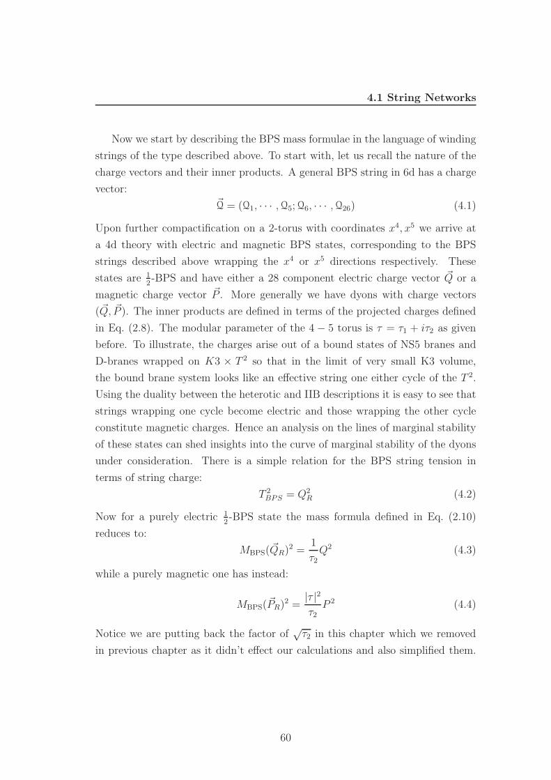
4.1 String Networks
Now we start by describing the BPS mass formulae in the language of winding
strings of the type described above. To start with, let us recall the nature of the
charge vectors and their inner products. A general BPS string in 6d has a charge
vector:~Q = (Q1, · · · , Q5; Q6, · · · , Q26) (4.1)
Upon further compactification on a 2-torus with coordinates x4, x5 we arrive at
a 4d theory with electric and magnetic BPS states, corresponding to the BPS
strings described above wrapping the x4 or x5 directions respectively. These
states are 12-BPS and have either a 28 component electric charge vector ~Q or a
magnetic charge vector ~P . More generally we have dyons with charge vectors
( ~Q, ~P ). The inner products are defined in terms of the projected charges defined
in Eq. (2.8). The modular parameter of the 4 − 5 torus is τ = τ1 + iτ2 as given
before. To illustrate, the charges arise out of a bound states of NS5 branes and
D-branes wrapped on K3 × T 2 so that in the limit of very small K3 volume,
the bound brane system looks like an effective string one either cycle of the T 2.
Using the duality between the heterotic and IIB descriptions it is easy to see that
strings wrapping one cycle become electric and those wrapping the other cycle
constitute magnetic charges. Hence an analysis on the lines of marginal stability
of these states can shed insights into the curve of marginal stability of the dyons
under consideration. There is a simple relation for the BPS string tension in
terms of string charge:
T 2BPS = Q2
R (4.2)
Now for a purely electric 12-BPS state the mass formula defined in Eq. (2.10)
reduces to:
MBPS( ~QR)2 =1
τ2
Q2 (4.3)
while a purely magnetic one has instead:
MBPS(~PR)2 =|τ |2τ2
P 2 (4.4)
Notice we are putting back the factor of√
τ2 in this chapter which we removed
in previous chapter as it didn’t effect our calculations and also simplified them.
60

4.1 String Networks
For the case when of a dyonic 12-BPS states having parallel vectors ~Q and ~P :
MBPS( ~QR, ~PR)2∣∣∣~QR‖~PR
=1
τ2( ~QR − τ ~PR) · ( ~QR − τ ~PR) (4.5)
Now the above formulae can be derived from the winding string picture by not-
ing that the minimum length of a string winding once round the electric (resp.
magnetic) direction is√
Aτ2
(resp.√
Aτ2|τ |) where A is the area of the 4-5 torus.
More generally, the length of a string winding q times along x4 and p times
along x5 is√
Aτ2|q + pτ | (in what follows, we will refer to such a string as a (p, q)
wound string). Now if the string in question has a charge vector ~QR, then when
it winds, the resulting BPS particle has electric and magnetic charge vectors~QR = q~QR, ~PR = −p~QR. From Eq. (4.2) we see that the BPS mass is:
MBPS(q~QR, p~QR) =
√A
τ2|q + pτ |
√Q2
=
√A
τ2
√( ~Q − τ ~P ) · ( ~Q − τ ~P ) (4.6)
which agrees with Eq. (4.5) upto an overall factor of√
A which is accounted for
by the relation between the metric in 6d and 4d. Henceforth we drop this factor
of√
A.
Let us now turn to the 14-BPS dyons. These have non-parallel charge vectors
~Q, ~P . The BPS mass formula for these is given by Eq. (2.10) The key point[3]
is that these correspond to BPS string junctions[21, 22] wrapped over the 4-5
torus. To see this, consider a junction where a string of charge vector ~Q1 and
another string of charge vector ~Q2 (not parallel to ~Q1) merge into a string of
charge ~Q1 + ~Q2 and then split back into the original constituents. (This is not
by any means the most general configuration, a point to which we will return
in the following section.) This can be extended to a periodic string network, in
other words one that can be wrapped on a 2-torus. The corresponding dyon has
electric and magnetic charge vectors:
~QR = ~Q1R, ~PR = −~Q2R (4.7)
Thus the BPS mass formula Eq. (2.10) becomes:
M2BPS =
1
τ2(~Q1R + τ ~Q2R) · (~Q1R + τ~Q2R) + 2
√∆(~Q1R, ~Q2R) (4.8)
61

4.1 String Networks
l3l1
l2
ω
ω1
2
l3
ω1
2ωl2
l1
θφ
Figure 4.1: A simple periodic network. Same network with a different basic cell.
which is more or less the same formula as before, but expressed in terms of the
charge vectors of two different BPS strings of the 6d theory.
Following [22, 40], this can be rewritten as the contribution of different seg-
ments of the junction. First of all, suppose that Re τ = τ1 = 0 and also the charge
vectors are orthogonal: ~Q1R · ~Q2R = 0. In this case the torus is rectangular and
the junction degenerates to a pair of intersecting strings (the intervening string
shrinks away), so we have:
mnetwork =
√1
τ2
(Q21R + S2Q2
2R) + 2|Q1R||Q2R|
=|~Q1R|√
τ2+√
τ2|~Q2R| (4.9)
A more general situation, where the torus is slanted but the junction is still
degenerate, arises for arbitrary τ1 if ~Q1 · ~Q2 = − τ1|τ | |~Q1||~Q2|. In this case we find
that:
mnetwork =|~Q1|√
τ2
+
√τ 21 + S2
τ2
|~Q2| (4.10)
Therefore the BPS mass is the sum of the BPS masses of two strings of charge
vectors ~Q1, ~Q2 that are separately wrapped on the electric and magnetic directions
to make 12-BPS particles. This is, in fact, a point of marginal stability.
Finally we consider the basic network of Fig.4.1. We want to show that MBPS
in Eq. (2.10) is equal to:
mnetwork = l1|~Q1| + l2|~Q2| + l3|~Q1 + ~Q2| (4.11)
62

4.1 String Networks
To see this, note that the generators of the torus ω1, ω2, are given by:
~ω1 = ~l1 −~l3
~ω2 = ~l2 −~l3 (4.12)
where the ~li are all outward-pointing vectors at the junction. Define the angles
θ, θ12, θ23, θ31 as follows:
~ω1 · ~ω2 = |~ω1||~ω2| cos θ
~l1 ·~l2 = l1 l2 cos θ12
~l2 ·~l3 = l2 l3 cos θ23
~l3 ·~l1 = l1 l3 cos θ31 (4.13)
satisfying θ12 + θ23 + θ31 = 2π.
Then the modular parameter τ and area A of the torus are:
τ =|~ω2||~ω1|
eiθ
A = |~ω1||~ω2| sin θ (4.14)
From the force balance condition for BPS string junctions, it follows that:
~Q1 · ~Q2 = |~Q1||~Q2| cos θ12
sin θ13|~Q1| = sin θ23|~Q2||~Q1 + ~Q2| = − cos θ31|~Q1| − cos θ32|~Q2| (4.15)
Inserting the above relations in Eq. (4.8) and dropping a factor of the area A
as before, we find:
M2BPS = (l21 + l23 − 2 l1 l3 cos θ13)Q
21 + (l22 + l23 − 2 l2 l3 cos θ23)Q
22
+2|~ω1||~ω2|(cos θ12 cos θ + sin θ12 sin θ)|~Q1||~Q2| (4.16)
It is easily shown that
|~ω1||~ω2|(cos θ12 cos θ + sin θ12 sin θ) = l1 l2 − l1 l3 cos θ23 − l2 l3 cos θ31 + l23 cos θ12
(4.17)
63

4.2 Classification of periodic string networks
and therefore
M2BPS = (l21 + l23 − 2 l1 l3 cos θ13)Q
21 + (l22 + l23 − 2 l2 l3 cos θ23)Q
22
+2(l1 l2 − l1 l3 cos θ23 − l2 l3 cos θ31 + l23 cos θ12
)|~Q1||~Q2| (4.18)
Finally, using Eq. (4.15), we end up with:
MBPS = l1|~Q1| + l2|~Q2| + l3|~Q1 + ~Q2| = mnetwork (4.19)
as desired.
From the above considerations we see that the 14-BPS state we have considered,
with charge vectors ~Q, ~P , is equivalent to a string junction made of three types
of strings with charge vectors ~Q1 = ~Q, ~Q2 = ~P and ~Q1 + ~Q2. In the following
sections we first examine the simplest junctions and study their possible modes
of marginal decay. Thereafter we generalize these considerations to include the
most general 14-BPS states and study a number of their properties.
4.2 Classification of periodic string networks
From the discussions of the previous section, classifying 14-BPS dyons amounts to
classifying all periodic string networks on the torus. Previous discussions of this
classification problem were mostly in the context of non-periodic networks with
infinitely extended external strings, see Refs.[39, 40]. Recently some aspects of
periodic networks were discussed in Ref.[11]. Below we will provide a complete
classification procedure for periodic string networks, in the process re-deriving
and extending some of the considerations in Ref.[11].
4.2.1 Some general properties
Start with a state with dyonic charge vector (~Q, ~P ). Because of the force-balance
condition, all the strings in the network must lie in the linear span of ~Q, ~P .
The corresponding string network, when inscribed on a torus, will have a net
number of strings of total charge ~Q winding around the x4 direction and another
number of strings of total charge ~P winding on the x5 direction. In the standard
representation of the torus as a parallelogram, the most convenient way to identify
64

4.2 Classification of periodic string networks
these charges is to add up the charge vectors of all the strings going “out” of the
parallelogram towards the right and the top respectively.
Suppose V, E, F are the total number of vertices, edges and faces in the net-
work. The fact that the network is on a torus means that V −E+F = 0. Suppose
also that the network is completely non-degenerate, meaning that all vertices are
three-string junctions (as opposed to the situation when a string degenerates to
zero length, in which case two three-point vertices merge to form a four-point
vertex, which should really be thought of as two strings crossing each other). It
follows that 2E = 3V . Therefore the number of vertices is always even and the
number of edges is a multiple of 3.
Next, write:
~Q = m~Q1, ~P = n~Q2 (4.20)
where m, n are the largest integer factors in ~Q, ~P respectively. As defined before
when m = n = 1 we call the dyon has unit torsion. The corresponding network
necessarily has a single string of charge ~Q1 going out towards the right of the
torus and a single string of charge ~Q2 going out towards the top. The unique way
to join these into a non-degenerate network is the one depicted in Fig.4.1. This
is a hexagonal network with V = 2, E = 3. It follows that all unit torsion string
networks on the torus are hexagonal. To make contact with the observations in
Ref.[11] we note that I in that reference is just mn in our discussion, therefore
the networks that we say have unit torsion are those having I = 11.
Arbitrary torsion networks have a more complicated structure. Suppose first
that (m, n) 6= (1, 1) and are relatively prime. We will refer to this case as an
irreducible 14-BPS dyon. At a generic point in moduli space, it is represented
by a non-degenerate string web with m strings of charge ~Q1 wrapping x4 and n
strings of charge ~Q2 wrapping x5. The total number of vertices in this network
is 2mn. One way to see this is that if the strings just cross each other forming a
completely degenerate network then we have mn four-point intersections, but in
the fully non-degenerate case each four-point intersection is blown up into a pair
of three-point vertices which are therefore 2mn in number. It also follows that
1In an M-theory lift they correspond to genus-2 surfaces. Here we focus primarily on the
string network representation.
65

4.2 Classification of periodic string networks
Figure 4.2: A dyon with charges 3~Q1, 2~Q2
the number of edges in an (m, n) network is 3mn. An example for (m, n) = (3, 2)
is shown in Fig.4.2, where one sees by inspection that there are 12 vertices and 18
edges. In this example we have assumed ~Q21 = ~Q2
2 and ~Q1 ·~Q2 = 0. The network is
not purely hexagonal, in fact it is made up of two types of rectangles, two types
of hexagons and two types of octagons.
Higher torsion networks necessarily have bosonic zero modes. These are vari-
ations in the lengths of one or more segments consistent with the periodicity of
the torus and not changing the mass of the state. For a general irreducible dyon
of charges (m~Q1, n~Q2) the number of bosonic zero modes is mn − 1. This comes
from the fact that the number of faces in an (m, n) network is F = mn and the
number of zero modes is F − 1[40]. It follows that only unit torsion networks do
not have zero modes.
4.2.2 Dual grid diagrams
The presence of zero modes means we need to quantize the system to correctly
count the states. Temporarily postponing this quantization issue, let us address
the following question: given dyonic charges m~Q1, n~Q2 and a fixed x4, x5 torus,
what are all the topologically distinct non-degenerate networks one can draw?
66

4.2 Classification of periodic string networks
Figure 4.3: Dual grid diagrams and networks for (m, n) = (1, 1)
This is a well-defined question. We have already seen that when (m, n) = (1, 1)
the topology is that of a hexagonal lattice and therefore unique. For the other
cases, a method to obtain all possible topologies can be found by adapting the
idea of dual grid diagrams[40] to the present case, which differs from the cases
considered in the older literature in two ways: (i) instead of two possible types of
strings (F and D) and their bound states, we have 26 types of strings and their
bound states, and (ii) the resulting networks are to be drawn on a torus.
We have seen that fixing the charges of a dyon amounts to choosing two unit
torsion charge vectors ~Q1, ~Q2 in terms of which the charges are represented as
m~Q1, n~Q2. Since BPS networks are planar, and the directions of the strings are
determined by the charge vectors, it follows that all charges appearing in a planar
BPS network are in the linear span (with integer coefficients) of ~Q1, ~Q2. Therefore
after fixing ~Q1, ~Q2, all possible networks and their degeneration can be understood
in terms of the two integers m, n. This essentially makes this problem similar to
the one of F- and D-string junctions for which dual grid diagrams were originally
proposed.
Now we address the more nontrivial issue of periodicity. Let us represent an
m, n dyon by a rectangular grid of m points by n points. The outer walls of the
rectangle are drawn as solid lines. Additional solid lines are drawn joining any
pair of points in the grid, but intersecting lines are not allowed. When no more
lines can be added, the diagram is called non-degenerate. In this case the interior
of the rectangle has been divided up into triangles. Degenerate diagrams can be
drawn by removing any subset of internal lines of a non-denegerate diagram. The
allowed non-degenerate dual grid diagrams for (1, 1) and (1, 2) dyons are shown
in Figs. 4.3, 4.4. Some of them are related to others by obvious symmetries. In
67

4.2 Classification of periodic string networks
Figure 4.4: Dual grid diagrams for (m, n) = (1, 2)
what follows, the grid diagrams of interest to us will always be the non-degenerate
ones.
Given such a diagram, a periodic network is constructed as follows. Draw
strings passing transversely through every line of the grid diagram. The charge
vector of each string coming in from the left is ~Q1 and of each one coming in
from the bottom is ~Q2. The remaining charge vectors can be assigned by charge
conservation at a vertex, or equivalently by noting that a line in the grid diagram
described by the 2-vector (n,−m) is crossed by an (m, n) string. Once a string
network has been drawn in this way we can forget about the original grid diagram.
We are left with an open string network (“open” in the sense that some strings
are emerging from it) with m strings of charge vector ~Q1 coming in from the left
and going out to the right, and n strings of charge vector ~Q2 coming in from below
and emerging at the top. This non-periodic network will constitute the unit cell
of a periodic network of strings.
Next we adjust the angles between the strings at every vertex to ensure force
balance. For much of the following discussion we will find it convenient to choose~Q1 · ~Q2 = 0 in which case the incoming and outgoing strings are either horizontal
or vertical, but the general case is not much more complicated. Some dual grid
diagrams and their corresponding open networks after performing this operation
are shown in Fig.4.5.
68

4.2 Classification of periodic string networks
Figure 4.5: Some grid diagrams and their corresponding networks, for (m, n) =
(1, 2)
Now we can allow the internal and external lengths in the open network to
vary. However, this variation must be consistent with the possibility of making
a periodic network out of the given open network. This restricts the number of
independent parameters, for which we now derive a formula.
Consider a dual grid diagram with m rows and n columns. We will show
that the total number of freely adjustable parameters consistent with making the
corresponding string network periodic is mn + 2.
Before doing this, we single out a class of special cases where all diagonals in
the network are ”simple”, namely they are created by joining a single horizontal
and a single vertical string. In the dual grid diagram this corresponds to all
diagonals lying at 45 degrees, or equivalently being diagonals of a unit square.
There are 2mn such grid diagrams, corresponding to an independent choice of
orientation of the diagonal in each unit square. An example of a “simple” grid
diagram is is shown in Fig 4.6.
69

4.2 Classification of periodic string networks
Figure 4.6: A simple and a non-simple 5 × 3 grid diagram.
More complicated diagonals in the network occur when a vertical or horizontal
string joins a diagonal one such that the outgoing string is slanted at more than
45 degrees. In the dual diagram this corresponds to diagonals that extend across
more than one unit square, as on the right hand side of Fig.4.6.
For the counting, let us start with the simplest of all (m, n) grid diagrams, in
which all diagonals are parallel. This, along with its accompanying open network
which is a hexagonal lattice, is illustrated in Fig.4.7. It is easy to count the number
of free parameters in the corresponding network. There are mn lines of each
type: horizontal, vertical and diagonal, making 3mn altogether. Incorporating
them into a network with fixed angles puts constraints on the lengths of these
3mn lines. We can think of these constraints as follows. In a given row there
is a set of n − 1 spacings between consecutive vertical lines. These must be
matched with those of the following row, leading to n − 1 constraints per row,
or m(n− 1) “row-type” constraints. Similarly there are n(m− 1) “column-type”
constraints. Finally when we make the open network periodic, we find constraints
on the external lines. The horizontal ones are all determined by the periodicity
requirement in terms of one horizontal line, making (m − 1) constraints, and
similarly there are (n− 1) constraints on the vertical ones. This exhausts all the
70

4.2 Classification of periodic string networks
Figure 4.7: The simplest (m, n) grid diagram.
constraints1. Thus we have:
3mn − m(n − 1) − n(m − 1) − (m − 1) − (n − 1) = mn + 2 (4.21)
as the final number of free parameters in a network of the type shown in Fig.4.7.
Turning now to more general, but still “simple”, grid diagrams as on the left
side of Fig.4.6, we notice that any such diagram can be obtained from the one
of Fig.4.7 by a series of “flops” which consist of individual diagonals within unit
squares being replaced by the opposite diagonals of these squares. These “flops”
can be thought of as a four-string junction inside the network having its inter-
mediate line shrink to zero and grow back with the opposite orientation. After
a flop, the number of adjustable parameters is the same as before since we have
merely replaced a diagonal by another one. In fact for all simple grid diagrams,
the counting can be done as before by identifying lengths and constraints, and
leads to the same result as for the simplest case.
Now let us turn to the most general case, like the one shown on the right hand
side of Fig.4.6. Although it seems less obvious, here too one can obtain the grid
diagram by a series of “flops” starting from the simplest one of Fig.4.7. This time
1In addition there is a discrete choice involving a cyclic permutation of the outgoing lines,
which will play an important role in what follows but is not relevant for parameter counting.
71

4.2 Classification of periodic string networks
1
2
1
2
Figure 4.8: A flop where a horizontal line is replaced by a diagonal.
the flops are not solely of the diagonals, but also of the horizontal and vertical
internal lines. An example of such a flop is depicted in Fig 4.8. We conclude
that all periodic m × n string networks have the same number of independent
parameters, namely mn + 2.
There is a useful check to this formula. If we try to inscribe a periodic network
with mn + 2 length parameters on a 2-torus, this fixes three parameters of the
network in terms of the three torus parameters: the complex modular parameter
and the area. That leaves mn − 1 free parameters for the toroidal network,
precisely equal to the number of zero modes that we have already determined.
It is worth mentioning here that the parameter space is bounded by the re-
quirement that all the lengths be positive or zero. The boundary is reached when
one or more strings shrink to zero length, causing a degeneration of some seg-
ment of the whole network into crossed strings. A “flop”, where a new string then
grows back with a different orientation, corresponds in some ways to a negative
length parameter, much like what happens at Calabi-Yau singularities.
72

4.2 Classification of periodic string networks
4.2.3 Periodic identifications
To complete our classification, we now need to address the issue of periodic iden-
tifications. For definiteness, consider the open network depicted in Fig.4.7. We
see that it has three strings emerging from top and bottom. To make a periodic
network out of this, we need to pairwise identify these strings. Clearly there
are three distinct ways to do this, which are just cyclic permutations of each
other. Similarly, when we identify the five horizontal strings at left with their
counterparts on the right, we encounter a five-fold choice corresponding to cyclic
permutations. In more generality, given a specific (m, n) grid diagram and its
associated open network, we want to ask how many ways this network can be
closed into a periodic one on a torus. The possible ways can be labelled by a pair
of integers (r, s), 0 ≤ r ≤ m, 0 ≤ s ≤ n. What we will see is that for a given dual
grid diagram, not all (r, s) lead to valid networks. The reason is that in some
cases the length constraints can only be solved by assigning a negative length to
one or more of the lines. In this case the given (non-degenerate) grid diagram
does not lead to a periodic network, though some “flopped” version of it may be
allowed, since as mentioned above, a negative length can typically be thought of
as a positive length after a flop.
Let us work this out in detail for the case of a (1, 3) network. This, with
all its length parameters labelled, is shown in Fig.4.9. Note that vij are to be
understood as the total lengths of the vertical lines after suitable identifications
of the upper and lower verticals. We have introduced√
2 factors in the definition
of the diagonal lengths to simplify the resulting formulae.
Let us make this periodic by identifying the first vertical line on the top with
the first one below. In terms of our previous notation this can be labelled as an
(r, s) = (0, 0) identification. The resulting constraint equations can be read off
from the figure, and are:
h12 + d11 = h12 + d12
h13 + d12 = h13 + d13
v11 + d11 = v12 + d12 = v13 + d13 (4.22)
73

4.2 Classification of periodic string networks
h
h
h
v v v
2 d
2 d
2 d
11
11
11 12
12
13
13
1312
Figure 4.9: A (1, 3) open network with labelled lengths.
As expected, these are 4 equations on 9 variables and they leave 5 independent
variables. These variables must be taken to be one diagonal (since all diagonals
are set equal), one vertical (for the same reason) and three horizontals, all of
which remain independent and arbitrary.
Now let us consider the next identification, in which the first line on the
top is identified with the second line below. In this case, which corresponds to
(r, s) = (0, 1), the equations are:
h12 + d11 = h13 + d13
h13 + d12 = h11 + d11
v11 + d11 + d12 = v12 + d12 + d13 = v13 + d13 + d11 (4.23)
This time we can arbitrarily choose, for example, three diagonals, one horizontal
and one vertical, or else three horizontals, one diagonal and one vertical.
Finally the identification obtained by matching the first line on top to the
third line below, namely (r, s) = (0, 2), leads to the equations:
h12 + d11 = h11 + d11
h13 + d12 = h12 + d12
v11 = v12 = v13 (4.24)
74

4.2 Classification of periodic string networks
hv
2 d
11
11
11 2 d
h13
122 d13
1312v v
12h
Figure 4.10: A different (1, 3) open network with labelled lengths.
This time all the verticals are equal and the remaining independent variables are
three diagonals and a horizontal or the other way around.
We see that all the periodic identifications are allowed for the particular open
network in Fig.4.9. However, if we choose a different network with the same
charges, as in Fig.4.10, then things will be rather different.
In this case, if we match the first vertical lines on top and bottom, the resulting
equations are:
h12 + d11 + d12 = h12
h13 = h13 + d12 + d13
v11 + d11 = v12 + d12 = v13 + d13 (4.25)
which has no solutions if we require all lengths to be positive. If we allow one
diagonal, say d12, to be negative then we can have solutions, but those will cor-
respond to the network of Fig.4.9 which we have already taken into account.
This only shows that the (r, s) = (0, 0) identification does not work for the
network of Fig.4.10. With (r, s) = (0, 1) we instead have:
h12 + d11 + d12 = h13 + d12 + d13
h13 = h11 + d11
v11 + d11 = v12 + d13 = v13 + d13 + d11 (4.26)
75

4.3 Discussion
which does admit sensible solutions, for example we can choose all the diagonals
independently along with one horizontal and one vertical length. Similarly one
can check that (r, s) = (0, 2) is also allowed.
We can generalize from this example to reach the following conclusions. First,
for every dual grid diagram and its corresponding open string network there are
several possible periodic networks, depending on the (r, s) shift in the identifi-
cation of vertical and horizontal external lines. Second, some of these may be
disallowed by the positivity condition on lengths.
4.3 Discussion
In this chapter we discussed the process of marginal decay of a 14-BPS in terms of
BPS string junctions. We showed how we arrive at the mass formula of a general
dyon by calculating the effective length of strings wrapping the T 2 for the basic
network. The marginal dyon decay is essentially the process when the length of
one of the strings in the string junction vanishes. Implementing this condition
on the torus modular parameter we arrive at the curve of marginal stability.
Classifying 14-BPS dyons amounts to classifying all periodic string networks on
the torus. We provided a complete classification procedure for periodic string
networks. For an arbitrary torsion network, this required us to study the dual
grid diagrams. For a given dual grid diagram, the force balance condition and
periodicity restricts the number of allowed topologically distinct non-degenerate
networks. We illustrated this fact using few higher torsion string networks.
76

Chapter 5
Kinematical Analogy for
Marginal Dyon Decay
Now we explore a kinematical analogy for the previously discussed marginal decay
of 14-BPS dyons in 4-dimensional N = 4 string compactifications. In this analogy,
the electric and magnetic charges play the role of spatial momenta, the BPS mass
plays the role of energy, and 12-BPS dyons correspond to massless particles. Using
SO(12, 1) “Lorentz” invariance and standard kinematical formulae in particle
physics, we provide simple derivations of the curves of marginal stability. We
also show how these curves map into the momentum ellipsoid, and propose some
applications of this analogy.
5.1 Introduction and review
The system and notations we will be working with are the same as that in the
previous chapters. we work in the duality frame corresponding to IIB compactifi-
cation on K3×T 2 or the heterotic string on T 6, the two being related by duality.
In what follows we will use the duality frame appropriate for type IIB. For pur-
poses of the BPS mass formula, the relevant inner products for the charge vectors
are:
Q2 ≡ ~QT (M + L) ~Q, P 2 ≡ ~P T (M + L) ~P , P · Q ≡ ~P T (M + L) ~Q (5.1)
77

5.1 Introduction and review
We define these right-moving projections of the charge vectors, ~QR, ~PR, by:
Q2R ≡ ~QT
R~QR = ~QT (M + L) ~Q = Q2 (5.2)
and similarly for the other inner products. In this way the moduli-dependent
inner product Eq. (5.1) for the charge vectors is replaced by a standard moduli-
independent product while the moduli-dependence is moved to the vectors them-
selves1. In what follows, we will not always write the suffix R, since the inner
products are by definition the same whether we are dealing with the projected or
unprojected vector. The BPS mass formula for general 14-BPS dyons is [18, 48, 10]
defined before Eq. (2.10), where τ is the modular parameter of the torus2.
5.1.1 Kinematic Analogy
The formula Eq. (2.10) has a striking analogy to the energy-momentum dispersion
relation for a relativistic point particle, E2 = ~p 2 + m2. In this analogy, the BPS
mass plays the role of the energy of the particle, while the dyonic charges play
the role of momenta:
~p =1√τ2
( ~Q − τ ~P ) (5.3)
Conservation of dyonic charge corresponds to momentum conservation in the
kinematical system. For this, it is crucial that τ be complex (in fact it has a
strictly positive imaginary part). Then conservation of the imaginary part of the
momentum is equivalent to conservation of the dyon’s magnetic charge, while the
real part ensures conservation of electric charge.
To complete the analogy, note that the condition of marginal stability in a
decay: MBPS = MBPS1 +MBPS
2 + · · · corresponds to energy conservation. Finally,
the mass of the analogue particle is√
2(∆( ~Q, ~P )
) 14. A 1
2-BPS dyon has its
electric and magnetic charge vectors proportional, so ∆(~Q, ~P ) = 0. It therefore
corresponds to a massless particle.
1This refers to all moduli other than those of the 2-torus, which are always displayed
explicitly and do not appear in the inner product.2Our conventions are those in Ref.[10] and differ by a factor of 1
√
τ2
from those in Ref[26].
78
5.1 Introduction and review
Because the momentum vector defined in Eq. (5.3) is complex, some care
must be taken in defining the inner product. As each of ~Q, ~P is effectively 6-
dimensional (recall that they are all projected using a moduli-dependent matrix,
as in Eq. (5.2)), one can convert the momenta to real vectors in a 12-dimensional
space with Lorentz group SO(12, 1). As we have noted, these Lorentz symmetries
are symmetries of the dispersion relation and the kinematics of the decay process,
but not of the underlying string theory.
This point can be clarified by considering a general dyonic particle having a
momentum ~k in the noncompact three-dimensional space. For such a particle
the full dispersion relation is:
E2 = ~k2+ (MBPS)2
= ~k2+
1
τ2( ~Q − τ ~P ) · ( ~Q − τ ~P ) + 2
√∆( ~Q, ~P ) (5.4)
If we restrict our attention to electrically charged particles, ~P = 0, the above
equation simplifies to:
E2 = ~k2+
1
τ2
~Q2 (5.5)
which can be thought of as the dispersion relation for either a massive particle
in 4d or a massless particle in 10d. This is the expected situation for a Kaluza-
Klein particle whose electric charges are momenta along the toroidal directions.
The dependence on the modulus τ , though present, is trivial in this case and can
be removed by rescaling the metric appropriately. However, once we introduce
magnetic charges as well then the dispersion relation is nontrivially τ -dependent
and also contains the ∆ factor. Now if we put ~k = 0 then we have the kinematic
analogy of interest in the present work.
To recover the curves of marginal stability, consider a general two-body decay
of a particle with energy-momentum (E, ~p ) into a pair of particles of energy-
momentum (E1, ~p 1) and (E2, ~p 2). There are two Lorentz frames that are useful:
the rest frame of the initial particle and the lab frame where the initial particle has
a given spatial momentum. By working in the rest frame, the Lorentz invariant
p · p1 is easily shown to be:
p · p1 =1
2(m2 + m2
1 − m22) (5.6)
79

5.1 Introduction and review
The same Lorentz invariant in the lab frame can be written:
p · p1 = m21 +
√~p 2
1 + m21
√~p 2
2 + m22 − ~p 1 · ~p 2 (5.7)
Equating the two, we have:
√~p 2
1 + m21
√~p 2
2 + m22 − ~p 1 · ~p 2 =
m2 − m21 − m2
2
2(5.8)
To apply this to the decay of a 14-BPS dyon, we make the substitution in
Eq. (5.3) as well as:
~p 1 =1√τ2
( ~Q1 − τ ~P1), ~p 2 =1√τ2
( ~Q2 − τ ~P2) (5.9)
to find:√
| ~Q1 − τ ~P1|2 + 2τ2
√∆1
√| ~Q2 − τ ~P2|2 + 2τ2
√∆2 − Re( ~Q1 − τ ~P1) · ( ~Q2 − τ ~P2)
= τ2(√
∆ −√
∆1 −√
∆2)(5.10)
where ∆i = ∆( ~Qi, ~Pi). For fixed charge vectors ~Qi, ~Pi and moduli matrix M this
is an equation for the torus modular parameter τ . In other words, this is the
general curve of marginal stability!
We can relate this to previously derived forms of the curve, as in [10, 15, 26].
First let us consider the case of decay of a primitive (gcd( ~Q∧ ~P ) = 1) 14-BPS dyon
into two 12-BPS dyons. In this case the product particles are massless. Moreover,
the charge vectors of the decay products are given by[10]:
~Q1 = a ~N1, ~P1 = c ~N1
~Q2 = b ~N2, ~P2 = d ~N2 (5.11)
where~N1 = d ~Q − b ~P , ~N2 = −c ~Q + a~P (5.12)
nd ad − bc = 1. Thus the equation reduces to:
|a − cτ ||b − dτ | |~N1|| ~N2|√
∆− Re (a − cτ)(b − dτ)
~N1 · ~N2√∆
= τ2 (5.13)
80

5.1 Introduction and review
Let
E = −~N1 · ~N2√
∆( ~N1, ~N2)(5.14)
It is easily checked that
√1 + E2 =
| ~N1|| ~N2|√∆( ~N1, ~N2)
(5.15)
Using the above equations and the fact that ∆( ~N1, ~N2) = ∆( ~Q, ~P ), the curve
becomes:
|a − cτ ||b − dτ |√
1 + E2 + Re (a − cτ)(b − dτ)E = τ2 (5.16)
Now one can take the second term to the right side and square both sides, where-
upon the resulting quartic (in τ) re-factorises into a perfect square of the familiar
Sen circle equation. However there is a neater way to proceed. The above equa-
tion is the same as:
|(a − cτ)(b − dτ)(E + i)| + Re(a − cτ)(b − dτ)(E + i) = 0 (5.17)
which is equivalent to the two conditions:
Im(a − cτ)(b − dτ)(E + i) = 0
Re(a − cτ)(b − dτ)(E + i) < 0 (5.18)
The first of these is directly the equation of the Sen circle:
(τ1 −
ad + bc
2cd
)2
+
(τ2 +
E
2cd
)2
=1
4c2d2(1 + E2) (5.19)
while the second one restricts us to the τ2 > 0 region of that circle.
Next consider decays into two 14-BPS dyons, or one 1
4-BPS and one 1
2-BPS
dyon. In this case the charges of the final states are parametrised as:
~Q1 = m1~Q + r1
~P , ~P1 = s1~Q + n1
~P
~Q2 = (m − m1) ~Q − r1~P , ~P2 = −s1
~Q + (n − n1)~P (5.20)
where the charges of the initial dyon are now (m~Q, n~P ) with gcd( ~Q ∧ ~P ) = 1.
81

5.1 Introduction and review
Substituting the above into Eq. (5.10), transposing the second term to the
right hand side and squaring, one find the earlier derived curve Eq. (2.21):
(τ1 −
m ∧ n
2ns1
)2
+
(τ2 +
E
2ns1
)2
=1
4n2s21
((m ∧ n)2 + 4mnr1s1 + E2
)(5.21)
where
E ≡ −~Q1 · ~P2 − ~Q2 · ~P1√
∆=
1√∆
(ms1 Q2 − nr1 P 2 − (m ∧ n)Q · P
)(5.22)
and m ∧ n = m1n2 −m2n1. This is the general curve of marginal stability found
in [26].
5.1.2 Momentum ellipsoid
For two-body decay of an unstable particle in the lab frame, the final-state particle
momenta are constrained to lie on an ellipsoid of revolution, obtained by rotating
an ellipse in the forward and transverse momenta p1,‖ and p1,⊥ along the azimuthal
angles around the beam axis. It is tempting to guess that the curve of marginal
stability coincides with this ellipse, We will see below that this is roughly true
but the relationship is more complicated than one might have expected.
Indeed this approach, in which p and p1 are treated as the independent vari-
ables, is not the easiest way to derive the curves of marginal stability, which in
fact we have already done in the previous section by treating the final-state mo-
menta p1, p2 as the independent variables. Nevertheless it is of some conceptual
interest to understand how the curves of marginal stability are related to the
momentum ellipsoid. One reason why the embedding we will obtain is rather
complicated is that the momentum of the initial particle (which determines one
axis of the ellipse) itself depends on the modular parameter τ .
To find the momentum ellipsoid, we first eliminate ~p 2 in Eq. (5.8) in favour
of ~p , ~p 1. Then, taking the second term to the right hand side and squaring, we
end up with the equation:
m2
(p1,‖ −
|~p |(m2 − m21 − m2
2)
2m2
)2
+ (~p 2 + m2) p21,⊥ =
1
4λ(m2, m2
1, m22)
(1 +
~p 2
m2
)
(5.23)
82

5.1 Introduction and review
where
λ(a, b, c) ≡ a2 + b2 + c2 − 2ab − 2bc − 2ca (5.24)
Here p1,‖ and p1,⊥ are the components of ~p1 along and transverse to the beam.
The momentum ellipsoid is the ellipse in Eq. (5.23) rotated about the beam axis.
For decays into two 12-BPS states, we put m1 = m2 = 0 and the momentum
ellipsoid simplifies considerably into:(p1,‖ − |~p |
2
)2
14(~p 2 + m2)
+p2
1,⊥14m2
= 1 (5.25)
Evidently the major axis of the ellipse is proportional to√
~p 2 + m2, which from
Eq. (5.3) is τ -dependent. Therefore the momentum ellipsoid itself varies with τ ,
and the curve of marginal stability is technically not a subspace of a particular
ellipsoid. This can be remedied by defining a new variable p1 via:
p1 ≡p1,‖ − |~p |
2√1 + ~p 2
m2
(5.26)
in terms of which the ellipse becomes a circle with a τ -independent radius:
p21 + p2
1,⊥ =1
4m2 (5.27)
From Eqs.(5.3),(5.9) we find:
p1,‖ =1√τ2
Re(( ~Q − τ ~P ) · ( ~Q1 − τ ~P1)
)
| ~Q − τ ~P |(5.28)
p1,⊥ =1√τ2
1
| ~Q − τ ~P |
√| ~Q − τ ~P |2| ~Q1 − τ ~P1|2 −
(Re ( ~Q − τ ~P ) · ( ~Q1 − τ ~P1)
)2
from which one obtains:
p1 =1√τ2
1
| ~Q − τ ~P |(ad + bc − 2cdτ1)Q
2 + (2abτ1 − (ad + bc)|τ |2)P 2 + (−2ab + 2cd|τ |2)Q · P√1τ2| ~Q − τ ~P |2 + 2
√∆( ~Q, ~P )
p1,⊥ =1√τ2
1
| ~Q − τ ~P |
√∆( ~Q, ~P )
√(Re (a − cτ)(b − dτ)
)2
+ (E2 + 1)τ 22 (5.29)
where E has been defined in Eq. (5.14). As promised, this is rather complicated.
One might hope to find a better parametrisation that leads to a simpler embed-
ding.
83

5.1 Introduction and review
5.1.3 Multiparticle decays and the issue of codimension
As is well known, kinematics alone does not determine whether a decay actually
takes place. In the present situation, an additional constraint is furnished by the
fact that a BPS particle cannot decay into a non-BPS final state. If we violate
this condition, the matrix element for the decay will vanish by supersymmetry.
In order for the particles in the final state to be BPS relative to each other,
it is known that ~Qi,R, ~Pi,R must lie in the same plane as ~QR, ~PR. Along with the
kinematics, this condition implies that all decays other than two-body decays into12-BPS particles occur on codimension ≥ 2 subspaces of moduli space, as noted
in Refs.[15, 26].
We can incorporate this property into the kinematical analogy. Let us impose
on our 12-dimensional space the structure of a linear symplectic manifold. Thus
there is a polarization - a closed, non-degenerate 2-form that divides the space into
6 electric and 6 magnetic directions, each one a Lagrangian subspace analogous
to coordinates and momenta in a phase space.
Consider a particle of arbitrary 12-momentum. We use the polarization to
divide this momentum into its electric and magnetic parts, each being a 6-vector.
Now consider the “diagonal” 6-manifold obtained by identifying the electric and
magnetic subspaces. In this 6-manifold, the linear span of the electric and mag-
netic parts of the 12-momentum defines a plane (if these 6-vectors are non-
parallel) or a line (if they are parallel). The former case is 14-BPS while the
latter is 12-BPS.
In a two-body decay, if the original particle defines a plane in the “diagonal”
space while the final particles define lines, then by momentum conservation the
BPS condition is automatically satisfied. If the final state particles are 12-BPS
but three or more in number, or if at least one of them is 14-BPS, then the
dimensionality of the subspace of the diagonal space spanned is at least three.
In this case, additional conditions on the moduli besides the marginal stability
condition are required to make the decay possible[15, 26]. The embedding of
codimension ≥ 2 curves in the full moduli space has, however, not yet been given
a precise description.
84

5.1 Introduction and review
5.1.4 Decay widths on marginal stability curves
The kinematical analogy suggests that one consider decay and scattering pro-
cesses involving dyons on curves of marginal stability. As a simple example,
consider an ensemble of 14-BPS dyons of a given charge, at a curve of marginal
stability for decay into two 12-BPS dyons. The ensemble will decay with a width
given by a formula analogous to the classic formula for decay of a particle of
mass m into two identical massless particles, which in three noncompact space
dimensions and in the rest frame of the decaying particle is (see for example
Ref.[34]):
Γ =1
32π~m|M|2 (5.30)
where M is the matrix element for the process.
To apply this formula to the present case the kinematics needs to be re-done
in the lab frame of the decaying particle, and in 12 dimensions. We also need to
take into account the quantization rule for the analogue momenta, inherited from
the quantization of the original electric and magnetic charges. Finally, the matrix
element M needs to be computed. It seems quite plausible that everything here is
computable in string theory. One can similarly consider scattering cross-sections
for dyons.
Discussion
We have presented an analogy that maps the marginal stability conditions for 14-
BPS dyons into energy-momentum conservation in an analogue particle problem
in 12+1 dimensions. 14-BPS states behave like massive particles and 1
2-BPS states
like massless particles. The analogy provides a simple way to understand curves
of marginal stability and useful both in deriving these curves in other situations
and in suggesting ways to think about physical processes involving 14-BPS dyons.
85

Chapter 6
Conclusions
In the thesis we extensively discussed the process of marginal decay of a 14BPS
dyonic states. We derived the curve of marginal stability in the torus moduli
space for the most general 14BPS dyon decay in N = 4 supersymmetric string
theory. Earlier works had shown that when the product dyons are 12BPS, the
decay happens across a curve of codimension 1 and hence it leads to a jump in
the entropy of the system. This was done for the case of original dyon having
unit torsion. Furthermore in the gravity description this jump can be accounted
for by appearance and disappearance of two centered small black holes . We
extended this to the most general case when either one or both the products can
be 14BPS dyon with the original dyon having arbitrary torsion and derived the
equation of curve of marginal stability for this process. Some solutions of our
equation turned out to be ”spurious”, in the sense that they described a possible
reverse decay instead of forward decay. We provided an algorithm to rule out
these reverse decay channels. For the case when both products are 12BPS, we
discovered a similarity of the marginal curves with well known mathematical
construction of Farey sequence and Ford circles. This helped us in establishing
the non-intersecting behaviour of the curves in the upper half plane. We analyzed
the marginal curves for the case of higher torsion. It was easy to produce example
for this case where we showed that the curves do intersect in the upper half plane.
The intersection point of these curves
In the next chapter we have obtained the complete set of constraint equations
on all the moduli of the theory for the 14BPS dyon decay to happen. These
86

constraints come from the condition that the initial and final dyons are mutually
supersymmetric. The initial and final dyons are made mutually supersymmetric
by bringing the planes of the final charge vectors to the plane formed by the
initial electric and magnetic charges. For the case when both the product dyons
are 12BPS, the charge vectors already lie in the same plane. Therefore because
of enough supersymmetry, there is only one constraint equation coming from the
mass conservation in this case and hence the curve of marginal stability is of
codimension 1. However when either one or both of the products are 14BPS, the
moduli are adjusted to bring their charge vectors in a plane. We derived the
most general set of these constraint equations on the moduli which are to be
satisfied for the marginal decay to happen. The number of constraints can be
any arbitrary number depending on the components on initial and final charges.
We showed that the maximum number of these constraint equation will be 9.
We also extended our analysis to the multi-centered decays, and found a relation
between the loci of marginal stability obtained in this way and the supergravity
constraints on pairwise separations of the centres of multi-centered black holes.
Studying the string networks provided us a deep insight about the dynamics of
marginal decay of a dyon. We showed how we arrive at the mass formula for a unit
torsion dyon. It was effectively the product of the string tension and the string
length in a basic cell. A string network wrapped on a torus is necessarily a periodic
network. We provided a classification procedure for such periodic networks. An
arbitrary torsion dyon is represented by a rather complicated string network, but
we can easily calculate the number of zero bosonic modes using the networks.
A counting problem would involve quantizing these zero bosonic modes which
we have not addressed in our work. Dual grid diagrams are useful tools while
studying the string network. For a given grid diagram number of topologically
distinct non-degenerate diagrams can be drawn. We explained the procedure of
constructing the periodic string networks for a given dual grid diagram.
Further we discussed an intriguing analogy between the decay of a 14BPS
dyon and that of an unstable particle in particle physics. This gave an alternative
approach to the problem of marginal dyon decay and we could derive the equation
of curve of marginal stability in much simpler way using this analogy.
87

References
[1] D. Shih, A. Strominger, and X. Yin, Recounting dyons in N = 4 string
theory, JHEP 10 (2006) 087, [hep-th/0505094].
[2] A. Strominger, C. Vafa, Microscopic origin of the Bekenstein-Hawking
entropy, Phys. Lett.D379(1996) 99–104, [hep-th/9601029].
[3] D. Gaiotto, Re-recounting dyons in N = 4 string theory, hep-th/0506249.
[4] D. P. Jatkar and A. Sen, Dyon spectrum in CHL models, JHEP 04 (2006)
018, [hep-th/0510147].
[5] J. R. David, D. P. Jatkar, and A. Sen, Product representation of dyon
partition function in CHL models, JHEP 06 (2006) 064, [hep-th/0602254].
[6] J. R. David and A. Sen, CHL dyons and statistical entropy function from
D1-D5 system, JHEP 11 (2006) 072, [hep-th/0605210].
[7] J. R. David, D. P. Jatkar, and A. Sen, Dyon spectrum in N = 4
supersymmetric type II string theories, JHEP 11 (2006) 073,
[hep-th/0607155].
[8] J. R. David, D. P. Jatkar, and A. Sen, Dyon spectrum in generic N = 4
supersymmetric Z(N) orbifolds, JHEP 01 (2007) 016, [hep-th/0609109].
[9] A. Dabholkar and D. Gaiotto, Spectrum of CHL dyons from genus-two
partition function, hep-th/0612011.
[10] A. Sen, Walls of marginal stability and dyon spectrum in N=4
supersymmetric string theories, hep-th/0702141.
88

REFERENCES
[11] A. Dabholkar, D. Gaiotto, and S. Nampuri, Comments on the spectrum of
CHL dyons, hep-th/0702150.
[12] N. Banerjee, D. P. Jatkar, and A. Sen, Adding charges to N = 4 dyons,
0705.1433.
[13] A. Sen, Two centered black holes and N=4 dyon spectrum, 0705.3874.
[14] M. C. N. Cheng and E. Verlinde, Dying dyons don’t count, 0706.2363.
[15] A. Sen, Rare decay modes of quarter BPS dyons, 0707.1563.
[16] R. Dijkgraaf, E. P. Verlinde, and H. L. Verlinde, Counting dyons in N = 4
string theory, Nucl. Phys. B484 (1997) 543–561, [hep-th/9607026].
[17] F. Denef and G. W. Moore, Split states, entropy enigmas, holes and halos,
hep-th/0702146.
[18] M. Cvetic and D. Youm, Dyonic bps saturated black holes of heterotic
string on a six torus, Phys. Rev. D53 (1996) 584–588, [hep-th/9507090].
[19] S. Lang, Algebra. Addison-Wesley, 1993.
[20] O. Aharony, A. Hanany, and B. Kol, Webs of (p,q) 5-branes, five
dimensional field theories and grid diagrams, JHEP 01 (1998) 002,
[hep-th/9710116].
[21] K. Dasgupta and S. Mukhi, BPS nature of 3-string junctions, Phys. Lett.
B423 (1998) 261–264, [hep-th/9711094].
[22] A. Sen, String network, JHEP 03 (1998) 005, [hep-th/9711130].
[23] T. Apostol, Modular Functions and Dirichlet Series in Number Theory.
Springer-Verlag, 1976.
[24] A. Sen, Black Hole Entropy Function, Attractors and Precision Counting of
Microstates, arXiv:0708.1270.
[25] F. Denef, Supergravity Flows and D-brane Stability, JHEP 08 (2000) 050,
[hep-th/0005049].
89

REFERENCES
[26] A. Mukherjee, S. Mukhi, and R. Nigam, Dyon Death Eaters, JHEP 10
(2007) 037, [arXiv:0707.3035].
[27] A. Mukherjee, S. Mukhi, and R. Nigam, Kinematical Analogy for Marginal
Dyon Decay, arXiv:0710.4533.
[28] J. Maharana and J. H. Schwarz, Noncompact Symmetries in String Theory,
Nucl. Phys. B390 (1993) 3–32, [hep-th/9207016].
[29] A. Sen, Electric Magnetic Duality in String Theory, Nucl. Phys. B404
(1993) 109–126, [hep-th/9207053].
[30] C. Wall, On the Orthogonal Groups of Unimodular Quadratic Forms, Math.
Annalen 147 (1962) 328.
[31] S. Banerjee and A. Sen, Duality Orbits, Dyon Spectrum and Gauge Theory
Limit of Heterotic String Theory on T 6, JHEP 03 (2008) 022,
[arXiv:0712.0043].
[32] E. Diaconescu and G. W. Moore, Crossing the Wall: Branes vs. Bundles,
arXiv:0706.3193.
[33] M. C. N. Cheng and E. P. Verlinde, Wall Crossing, Discrete Attractor
Flow, and Borcherds Algebra, arXiv:0806.2337.
[34] D. J. Griffiths, Introduction to elementary particles. Wiley, New York, 1987.
[35] J. Distler, A. Hanany (0,2) noncritical strings in six dimensions , Nucl.
Phys. B490 (1997) 75–90, [hep-th/9611104].
[36] A. Sen, String string duality conjecture in six-dimensions and charged
solitonic strings , Nucl. Phys. B450 (1995) 103–114, [hep-th/9504027].
[37] J. Harvey, A. Strominger, The heterotic string is a soliton , Nucl. Phys.
B449 (1995) 535–552, [hep-th/9504047].
[38] E. Witten, String theory dynamics in various dimensions , Nucl. Phys.
B443 (1995) 85–126, [hep-th/9503124].
90

REFERENCES
[39] O. Bergman, Three-pronged strings and 1/4 BPS states in N = 4
super-Yang-Mills theory , Nucl. Phys. B525 (1998) 104–116,
[hep-th/9712211].
[40] O. Bergman, B. Kol, String webs and 1/4 BPS monopoles , Nucl. Phys.
B536 (1998) 149–174, [hep-th/9804160].
[41] A. Dabholkar, D. Gaiotto, S. Nampuri, Comments on the spectrum of
CHL dyons , [hep-th/0702150].
[42] A. Dabholkar, D. Gaiotto, S. Nampuri Comments on the spectrum of CHL
dyons , [hep-th/0612011].
[43] K. Dasgupta, S. Mukhi, Orbifolds of M-theory , Nucl. Phys. B465 (1996)
399–412, [hep-th/9512196].
[44] E. Witten, Five-branes and M-theory on an orbifold , Nucl. Phys. B463
(1996) 383–397, [hep-th/9512219].
[45] H. Ooguri, A. Strominger, C. Vafa , Black hole attractors and the
topological string , Phys. Rev. D70 (2004) 106007, [hep-th/0405146].
[46] H. Ooguri, C. Vafa, E. P. Verlinde , Hartle-Hawking wave-function for flux
compactifications , Lett. Math. Phys. 74 (2005) 311-342, [hep-th/0502211].
[47] T. J. Hollowood, A. Iqbal, C. Vafa , Matrix Models, Geometric
Engineering and Elliptic Genera , [hep-th/0310272].
[48] M. J. Duff, J. T. Liu, J. Rahmfeld , Four-dimensional string-string-string
triality , Nucl. Phys. B459 (1996) 125–159, [hep-th/9508094].
91