debacl: a python package for interactive density … · 2 debacl: a python package for interactive...

JSSJournal of Statistical Software

MMMMMM YYYY, Volume VV, Issue II. http://www.jstatsoft.org/

DeBaCl: A Python Package for Interactive

DEnsity-BAsed CLustering

Brian P. KentCarnegie Mellon University

Alessandro RinaldoCarnegie Mellon University

Timothy VerstynenCarnegie Mellon University

Abstract

The level set tree approach of Hartigan (1975) provides a probabilistically based andhighly interpretable encoding of the clustering behavior of a dataset. By representing thehierarchy of data modes as a dendrogram of the level sets of a density estimator, thisapproach offers many advantages for exploratory analysis and clustering, especially forcomplex and high-dimensional data. Several R packages exist for level set tree estimation,but their practical usefulness is limited by computational inefficiency, absence of inter-active graphical capabilities and, from a theoretical perspective, reliance on asymptoticapproximations. To make it easier for practitioners to capture the advantages of level settrees, we have written the Python package DeBaCl for DEnsity-BAsed CLustering. Inthis article we illustrate how DeBaCl’s level set tree estimates can be used for difficultclustering tasks and interactive graphical data analysis. The package is intended to pro-mote the practical use of level set trees through improvements in computational efficiencyand a high degree of user customization. In addition, the flexible algorithms implementedin DeBaCl enjoy finite sample accuracy, as demonstrated in recent literature on densityclustering. Finally, we show the level set tree framework can be easily extended to dealwith functional data.

Keywords: density-based clustering, level set tree, Python, interactive graphics, functionaldata analysis.

1. Introduction

Clustering is one of the most fundamental tasks in statistics and machine learning, and nu-merous algorithms are available to practitioners. Some of the most popular methods, suchas K-means (MacQueen 1967; Lloyd 1982) and spectral clustering (Shi and Malik 2000), rely

arX

iv:1

307.

8136

v1 [

stat

.ME

] 3

0 Ju

l 201

3

http://www.jstatsoft.org/

2 DeBaCl: A Python Package for Interactive DEnsity-BAsed CLustering

on the key operational assumption that there is one optimal partition of the data into Kwell-separated groups, where K is assumed to be known a priori. While effective in somecases, this flat or scale-free notion of clustering is inadequate when the data are very noisy orcorrupted, or exhibit complex multimodal behavior and spatial heterogeneity, or simply whenthe value of K is unknown. In these cases, hierarchical clustering affords a more realistic andflexible framework in which the data are assumed to have multi-scale clustering features thatcan be captured by a hierarchy of nested subsets of the data. The expression of these subsetsand their order of inclusions—typically depicted as a dendrogram—provide a great deal ofinformation that goes beyond the original clustering task. In particular, it frees the practi-tioner from the requirement of knowing in advance the “right” number of clusters, provides auseful global summary of the entire dataset, and allows the practitioner to identify and focuson interesting sub-clusters at different levels of spatial resolution.

There are, of course, myriad algorithms just for hierarchical clustering. However, in most casestheir usage is advocated on the basis of heuristic arguments or computational ease, ratherthan well-founded theoretical guarantees. The high-density hierarchical clustering paradigmput forth by Hartigan (1975) is an exception. It is based on the simple but powerful definitionof clusters as the maximal connected components of the super-level sets of the probabilitydensity specifying the data-generating distribution. This formalization has numerous advan-tages: (1) it provides a probabilistic notion of clustering that conforms to the intuition thatclusters are the regions with largest probability to volume ratio; (2) it establishes a direct linkbetween the clustering task and the fundamental problem of nonparametric density estima-tion; (3) it allows for a clear definition of clustering performance and consistency (Hartigan1981) that is amenable to rigorous theoretical analysis and (4) as we show below, the den-drogram it produces is highly interpretable, offers a compact yet informative representationof a distribution, and can be interactively queried to extract and visualize subsets of dataat desired resolutions. Though the notion of high-density clustering has been studied forquite some time (Polonik 1995), recent theoretical advances have further demonstrated theflexibility and power of density clustering. See, for example, Rinaldo, Singh, Nugent, andWasserman (2012); Rinaldo and Wasserman (2010); Kpotufe and Luxburg (2011); Chaudhuriand Dasgupta (2010); Steinwart (2011); Sriperumbudur and Steinwart (2012); Lei, Robins,and Wasserman (2013); Balakrishnan, Narayanan, Rinaldo, Singh, and Wasserman (2013)and the refences therein.

This paper introduces the Python package DeBaCl for efficient and statistically-principledDEnsity-BAsed CLustering. DeBaCl is not the first implementation of level set tree estimationand clustering; the R packages denpro (Klemela 2004), gslclust (Stuetzle and Nugent 2010),and pdfCluster (Azzalini and Menardi 2012) also contain various level set tree estimators.However, they tend to be too inefficient for most practical uses and rely on methods lackingrigorous theoretical justification. The popular nonparametric density-based clustering algo-rithm DBSCAN (Ester, Kriegel, and Xu 1996) is implemented in the R package fpc (Hennig2013) and the Python library scikit-learn (Pedregosa, Varoquaux, Gramfort, Michel, Thirion,Grisel, Blondel, Prettenhofer, Weiss, Dubourg, Vanderplas, Passos, Cournapeau, Brucher,Perrot, and Duchesnay 2011), but this method does not provide an estimate of the level settree.

DeBaCl handles much larger datasets than existing software, improves computational speed,

Journal of Statistical Software 3

and extends the utility of level set trees in three important ways: (1) it provides several novelvisualization tools to improve the readability and interpetability of density cluster trees; (2) itoffers a high degree of user customization; and (3) it implements several recent methodologicaladvances. In particular, it enables construction of level set trees for arbitrary functions over adataset, building on the idea that level set trees can be used even with data that lack a bonafide probability density fuction. DeBaCl also includes the first practical implementation ofthe recent, theoretically well-supported algorithm from Chaudhuri and Dasgupta (2010).

2. Level set trees

Suppose we have a collection of points Xn = {x1, . . . , xn} in Rd, which we model as i.i.d.draws from an unknown probability distribution with probability density function f (withrespect to Lebesgue measure). Our goal is to identify and extract clusters of Xn without anya priori knowledge about f or the number of clusters. Following the statistically-principledapproach of Hartigan (1975), clusters can be identified as modes of f . For any threshold valueλ ≥ 0, the λ-upper level set of f is

Lλ(f) = {x ∈ Rd : f(x) ≥ λ}. (1)

The connected components of Lλ(f) are called the λ-clusters of f and high-density clustersare λ-clusters for any value of λ. It is easy to see that λ-clusters associated with larger valuesof λ are regions where the ratio of probability content to volume is higher. Also note thatfor a fixed value of λ, the corresponding set of clusters will typically not give a partition of{x : f(x) ≥ 0}.

The level set tree is simply the set of all high-density clusters. This collection is a tree becauseit has the following property: for any two high-density clusters A and B, either A is a subsetof B, B is a subset of A, or they are disjoint. This property allows us to visualize the levelset tree with a dendrogram that shows all high-density clusters simultaneously and can bequeried quickly and directly to obtain specific cluster assignments. Branching points of thedendrogram correspond to density levels where two or more modes of the pdf, i.e. new clusters,emerge. Each vertical line segment in the dendrogram represents the high-density clusterswithin a single pdf mode; these clusters are all subsets of the cluster at the level where themode emerges. Line segments that do not branch are considered high-density modes, whichwe call the leaves of the tree. For simplicity, we tend to refer to the dendrogram as the levelset tree itself.

Because f is unknown, the level set tree must be estimated from the data. Ideally we woulduse the high-density clusters of a suitable density estimate f to do this; for a well-behaved fand a large sample size, f is close to f with high probability so the level set tree for f wouldbe a good estimate for the level set tree of f (Chaudhuri and Dasgupta 2010). Unfortunately,this approach is not computationally feasible even for low-dimensional data because findingthe upper level sets of f requires evaluating the function on a dense mesh and identifyingλ-clusters requires a combinatorial search over all possible paths connecting any two pointsin the mesh.

Many methods have been proposed to overcome these computational obstacles. The first


category includes techniques that remain faithful to the idea that clusters are regions of thesample space. Members of this family include histogram-based partitions (Klemela 2004),binary tree partitions (Klemela 2005) (implemented in the R package denpro) and Delaunaytriangulation partitions (Azzalini and Torelli 2007) (implemented in R package pdfCluster).These techniques tend to work well for low-dimension data, but suffer from the curse ofdimensionality because partitioning the sample space requires an exponentially increasingnumber of cells or algorithmic complexity (Azzalini and Torelli 2007).

In contrast, another family of estimators produces high-density clusters of data points ratherthan sample space regions; this is the approach taken by our package. Conceptually, thesemethods estimate the level set tree of f by intersecting the level sets of f with the samplepoints Xn and then evaluating the connectivity of each set by graph theoretic means. Thistypically consists of three high-level steps: estimation of the probability density f(x) from thedata; construction of a graph G that describes the similarity between each pair of data points;and a search for connected components in a series of subgraphs of G induced by removingnodes and/or edges of insufficient weight, relative to various density levels.

The variations within the latter category are found in the definition of G, the set of densitylevels over which to iterate, and the way in which G is restricted to a subgraph for a givendensity level λ. Edge iteration methods assign a weight to the edges of G based on theproximity of the incident vertices in feature space (Chaudhuri and Dasgupta 2010) or thevalue of f(x) at the incident vertices (Wong and Lane 1983) or on a line segment connectingthem (Stuetzle and Nugent 2010). For these procedures, the relevant density levels are theedge weights of G. Frequently, iteration over these levels is done by initializing G withan empty edge set and adding successively more heavily weighted edges, in the manner oftraditional single linkage clustering. In this family, the Chaudhuri and Dasgupta algorithm(which is a generalization of Wishart (1969)) is particularly interesting because the authorsprove finite sample rates for convergence to the true level set tree (Chaudhuri and Dasgupta2010). To the best of our knowledge, however, only Stuetzle and Nugent (2010) has a publiclyavailable implementation, in the R package gslclust.

Point iteration methods construct G so the vertex for observation xi is weighted accordingto f(xi), but the edges are unweighted. In the simplest form, there is an edge between thevertices for observations xi and xj if the distance between xi and xj is smaller than somethreshold value, or if xi and xj are among each other’s k-closest neighbors (Kpotufe andLuxburg 2011; Maier, Hein, and von Luxburg 2009). A more complicated version places anedge (xi, xj) in G if the amount of probability mass that would be needed to fill the valleysalong a line segment between xi and xj is smaller than a user-specified threshold (Menardiand Azzalini 2013). The latter method is available in the R package pdfCluster.

3. Implementation

The default level set tree algorithm in DeBaCl is described in Algorithm 1, based on themethod proposed by Kpotufe and Luxburg (2011) and Maier et al. (2009). For a sample with


n observations in Rd, the k-nearest neighbor (kNN) density estimate is:

f(xj) =k

n · vd · rdk(xj)(2)

where vd is the volume of the Euclidean unit ball in Rd and rk(xj) is the Euclidean distancefrom point xj to its k’th closest neighbor. The process of computing subgraphs and findingconnected components of those subgraphs is implemented with the igraph package (Csardi andNepusz 2006). Our package also depends on the NumPy and SciPy packages for basic compu-tation (Jones, Oliphant, and Peterson 2001) and the Matplotlib package for plotting (Hunter2007). We use this algorithm because it is straightforward and fast; although it does require

Algorithm 1: Baseline DeBaCl level set tree estimation procedure

Input: {x1, . . . , xn}, k, γ

Output: T , a hierarchy of subsets of {x1, . . . , xn}

G← k-nearest neighbor similarity graph on {x1, . . . , xn};f(·)← k-nearest neighbor density estimate based on {x1, . . . , xn};for j ← 1 to n do

λj ← f(xj);

Lλj ← {xi : f(xi) ≥ λj};Gj ← subgraph of G induced by Lj ;

Find the connected components of Gλj ;

T ← dendrogram of connected components of graphs G1, . . . , Gn, ordered by inclusions;

T ← remove components of size smaller than γ;

return T

computation of all(n2

)pairwise distances, the procedure can be substantially shortened by

estimating connected components on a sparse grid of density levels. The implementation ofthis algorithm is novel in its own right (to the best of our knowledge), and DeBaCl includesseveral other new visualization and methodological tools.

3.1. Visualization tools

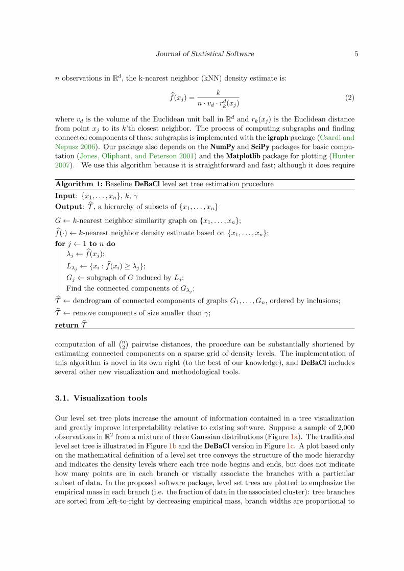
Our level set tree plots increase the amount of information contained in a tree visualizationand greatly improve interpretability relative to existing software. Suppose a sample of 2,000observations in R2 from a mixture of three Gaussian distributions (Figure 1a). The traditionallevel set tree is illustrated in Figure 1b and the DeBaCl version in Figure 1c. A plot based onlyon the mathematical definition of a level set tree conveys the structure of the mode hierarchyand indicates the density levels where each tree node begins and ends, but does not indicatehow many points are in each branch or visually associate the branches with a particularsubset of data. In the proposed software package, level set trees are plotted to emphasize theempirical mass in each branch (i.e. the fraction of data in the associated cluster): tree branchesare sorted from left-to-right by decreasing empirical mass, branch widths are proportional to


empirical mass, and the white space around the branches is proportional to empirical mass.For matching tree nodes to the data, branches can be colored to correspond to high-densitydata clusters (Figures 1c and 1d). Clicking on a tree branch produces a banner that indicatesthe start and end levels of the associated high-density cluster as well as its empirical mass(Figure 5a).

The level set tree plot is an excellent tool for interactive exploratory data analysis because itacts as a handle for identifying and plotting spatially coherent, high-density subsets of data.The full power of this feature can be seen clearly with the more complex data of Section 4.

(a) (b)

(c) (d)

Figure 1: Level set tree plots and cluster labeling for a simple simulation. A level set tree isconstructed from a sample of 2,000 observations drawn from a mix of three Gaussians in R2.a) The kNN density estimator evaluated on the data. b) A plot of the tree based only on themathematical definition of level set trees. c) The new level set tree plot, from DeBaCl. Treebranches emphasize empirical mass through ordering, spacing, and line width, and they arecolored to match the cluster labels in d. A second vertical axis is added that indicates thatfraction of background mass at each critical density level. d) Cluster labels from the all-modelabeling technique, where each leaf of the level set tree is designated as a cluster.


3.2. Alternate scales

By construction, the nodes of a level set tree are indexed by density levels λ, which determinethe scale of the vertical axis in a plot of the tree. While this does encode the parent-childrelationships in the tree, interpretability of the λ scale is limited by the fact that it dependson the height of the density estimate f . It is not clear, for example, whether λ = 1 would bea low- or a high-density threshold; this depends on the particular distribution.

To remove the scale dependence we can instead index level set tree nodes based on theprobability content of upper level sets. Specifically, let α be a number between 0 and 1 anddefine

λα = sup

{λ :

∫x∈Lλ(f)

f(x)dx ≥ α

}(3)

to be the value of λ for which the upper level set of f has probability content no smallerthan α (Rinaldo et al. 2012). The map α 7→ λα gives a monotonically decreasing one-to-onecorrespondence between values of α in [0, 1] and values of λ in [0,maxx f(x)]. In particular,λ1 = 0 and λ0 = maxx f(x). For an empirical level set tree, set λα to the α-quantile of{f(xi)}ni=1. Expressing the height of the tree in terms of α instead of λ does not changethe topology (i.e. number and ordering of the branches) of the tree; the re-indexed tree is adeformation of the original tree in which some of its nodes are stretched out and others arecompressed.

α-indexing is more interpretable and useful for several reasons. The α level of the tree indexesclusters corresponding to the 1 − α fraction of “most clusterable” data points; in particular,larger α values yield more compact and well-separated clusters, while smaller values can beused for de-noising and outlier removal. Because α is always between 0 and 1, scaling byprobability content also enables comparisons of level set trees arising from data sets drawnfrom different pdfs, possibly in spaces of different dimensions. Finally, the α-index is moreeffective than λ-indexing in representing regions of large probability content but low densityand is less affected by small fluctuations in density estimates.

A common (incorrect) intuition when looking at an α-indexed level set tree plot is to interpretthe height of the branches as the size of the corresponding cluster, as measured by its empiricalmass. However, with α-indexing the height of any branch depends on its empirical mass aswell as the empirical mass of all other branches that coexist with it. In order to obtain treesthat do conform to this intuition, we introduce the κ-indexed level set tree.

Recall from Section 2 that clusters are defined as maximal connected components of thesets Lλ(f) (see equation 1) as λ varies from 0 to maxx f(x), and that the level set tree isthe dendrogram representing the hierarchy of all clusters. Assume the tree is binary andwith tooted. Let {1, 2, . . . ,K} be an enumeration of the nodes of the level set tree and letC = {C0, . . . , CK} be the corresponding clusters. We can always choose the enumeration ina way that is consistent with the hierarchy of inclusions of the elements of C; that is, C0 isthe support of f (which we assume for simplicity to be a connected set) and if Ci ⊂ Cj , theni > j. For a node i > 0, we denote with parenti the unique node j such that Cj is the smallestelement of C such that Cj ⊃ Ci. Similarly, kidi is the pair of nodes (j, j′) such that Cj and


Cj′ are the maximal subsets of Ci. Finally, for i > 0, sibi is the node j such there exists a kfor which kidk = (i, j). For a cluster Ci ∈ C, we set

Mi =

∫Ci

f(x)dx, (4)

which we refer to as the mass of Ci.

The true κ-tree can be defined recursively by associating with each node i two numbers κ′iand κ′′i such that κ′i − κ′′i is the salient mass of node i. For leaf nodes, the salient mass is themass of the cluster, and for non-leaves it is the mass of the cluster boundary region. κ′ andκ′′ are defined differently for each node type.

1. Internal nodes, including the root node.

κ′0 = M0 = 1,

κ′i = κ′′parenti

κ′′i =∑j∈kidi

Mj +∑k∈sibi

Mk

2. Leaf nodes.

κ′i = κ′′parentiκ′′i = κ′i −Mi

To estimate the κ-tree, we use f instead of f and let mi be the fraction of data contained inthe cluster for the tree node i at birth. Again, define the estimated tree recursively:

κ′0 = 1,

κ′i = κ′′parenti ,

κ′′i = κ′i −mi +∑j∈kidi

mj .

In practice we subtract the above quantities from 1 to get an increasing scale that matchesthe λ and κ scales.

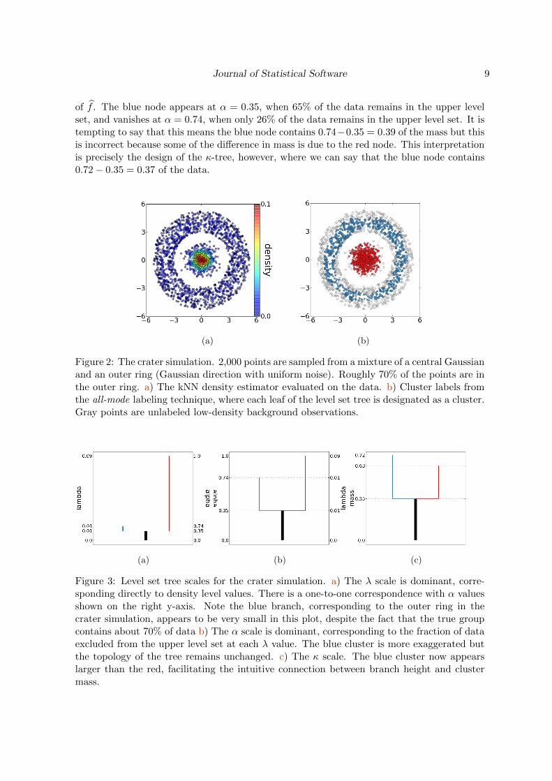
Note that switching between the λ to α index does not change the overall shape of the tree,but switching to the κ index does. In particular, the tallest leaf of the κ tree correspondsto the cluster with largest empirical mass. In both the λ and α trees, on the other hand,leaves correspond to clusters composed of points with high density values. The differencecan be substantial. Figure 3 illustrates the differences between the three types of indexingfor the “crater” example in Figure 2. This example consists of a central Gaussian with highdensity and low mass surrounded by a ring with high mass but uniformly low density. Theλ-scale tree (Figure 3a) correctly indicates the heights of the modes of f , but tends to producethe incorrect intuition that the ring (blue node and blue points in Figure 2b) is small. Theα-scale plot (Figure 3b) ameliorates this problem by indexing node heights to the quantiles


of f . The blue node appears at α = 0.35, when 65% of the data remains in the upper levelset, and vanishes at α = 0.74, when only 26% of the data remains in the upper level set. It istempting to say that this means the blue node contains 0.74−0.35 = 0.39 of the mass but thisis incorrect because some of the difference in mass is due to the red node. This interpretationis precisely the design of the κ-tree, however, where we can say that the blue node contains0.72− 0.35 = 0.37 of the data.

(a) (b)

Figure 2: The crater simulation. 2,000 points are sampled from a mixture of a central Gaussianand an outer ring (Gaussian direction with uniform noise). Roughly 70% of the points are inthe outer ring. a) The kNN density estimator evaluated on the data. b) Cluster labels fromthe all-mode labeling technique, where each leaf of the level set tree is designated as a cluster.Gray points are unlabeled low-density background observations.

(a) (b) (c)

Figure 3: Level set tree scales for the crater simulation. a) The λ scale is dominant, corre-sponding directly to density level values. There is a one-to-one correspondence with α valuesshown on the right y-axis. Note the blue branch, corresponding to the outer ring in thecrater simulation, appears to be very small in this plot, despite the fact that the true groupcontains about 70% of data b) The α scale is dominant, corresponding to the fraction of dataexcluded from the upper level set at each λ value. The blue cluster is more exaggerated butthe topology of the tree remains unchanged. c) The κ scale. The blue cluster now appearslarger than the red, facilitating the intuitive connection between branch height and clustermass.


3.3. Cluster retrieval options

Many clustering algorithms are designed to only output a partition of the data, whose elementsare then taken to be the clusters. As we argued in the introduction, such a paradigm isoften inadequate for data exhibiting complex and multi-scale clustering features. In contrast,hierarchical clustering in general and level set tree clustering in particular give a more completeand informative description of the clusters in a dataset. However, many applications requirethat each data point be assigned to a single cluster label. Much of the work on level settrees ignores this phase of a clustering application or assumes that labels will be assignedaccording to the connected components at a chosen λ (density) or α (mass) level, whichDeBaCl accomodates through the upper set clustering option. Rather than choosing a singledensity level, a practitioner might prefer to specify the number of clusters K (as with K-means). One way (of many) that this can be done is to find the first K − 1 splits in the levelset tree and identify each of the children from these splits as a cluster, known in DeBaCl asthe first-K clustering technique. A third, preferred, option avoids the choice of λ, α, or Kaltogether and treats each leaf of the level set tree as a separate cluster (Azzalini and Torelli2007). We call this the all-mode clustering method. Use of these labeling options is illustratedin Section 4.

Note that each of these methods assigns only a fraction of points to clusters (the foregroundpoints), while leaving low-density observations (background points) unlabeled. Assigning thebackground points to clusters can be done with any classification algorithm, and DeBaClincludes a handful of simple options, including a k-nearest neighbor classifer, for the task.

3.4. Chaudhuri and Dasgupta algorithm

Chaudhuri and Dasgupta (2010) introduce an algorithm for estimating a level set tree that isparticularly notable because the authors prove finite-sample convergence rates (where consis-tency is in the sense of Hartigan (1981)). The algorithm is a generalization of single linkage,reproduced here for convenience in Algorithm 2. To translate this program into a practical

Algorithm 2: Chaudhuri and Dasgupta (2010) level set tree estimation procedure.

Input: {x1, . . . , xn}, k, α

Output: T , a hierarchy of subsets of {x1, . . . , xn}

rk(xi)← distance to the k’th neighbor of xi;

for r ← 0 to ∞ doGr ← graph with vertices {xi : rk(xi) ≤ r} and edges {(xi, xj) : ‖xi − xj‖ ≤ αr};Find the connected components of Gλr ;

T ← dendrogram of connected components of graphs Gr, ordered by inclusions;

return T

implementation, we must find a finite set of values for r such that the graph Gr can onlychange at these values. When α = 1, the only values of r where the graph can change are the


edge lengths in the graph eij = ‖xi − xj‖ for all i and j. Let r take on each value of eij indescending order; in each iteration remove vertices and edges with larger k-neighbor radiusand edge length, respectively.

When α 6= 1, the situation is trickier. First, note that including r values where the graph doesnot change is not a problem, since the original formulation of the method includes all valuesof r ∈ R+0. Clearly, the vertex set can still change at any edge length eij . The edge set canonly change at values where r = eij/α for some i, j. Suppose eu,v and er,s are consecutivevalues in a descending ordered list of edge lengths. Let r = e/α, where eu,v < e < er,s.Then the edge set E = {(xi, xj) : ‖xi − xj‖ ≤ αr = e} does not change as r decreases untilr = eu,v/α, where the threshold of αr now excludes edge (xu, xv). Thus, by letting r iterateover the values in

⋃i,j{eij ,

eijα }, we capture all possible changes in Gr.

In practice, starting with a complete graph and removing one edge at a time is extremelyslow because this requires 2∗

(n2

)connected component searches. The DeBaCl implementation

includes an option to initialize the algorithm at the k-nearest neighbor graph instead, whichis a substantially faster approximation to the Chaudhuri-Dasgupta method. This shortcut isstill dramatically slower than DeBaCl’s geometric tree algorithm, which is one reason why weprefer the latter. Future development efforts will focus on improvements in the speed of bothprocedures.

3.5. Pseudo-densities for functional data

The level set tree estimation procedure in Algorithm 1 can be extended to work with datasampled from non-Euclidean spaces that do not admit a well-defined pdf. The lack of adensity function would seem to be an insurmountable problem for a method defined on thelevels of a pdf. In this case, however, level set trees can be built on the levels of a pseudo-density estimate that measures the similarity of observations and the overall connectivity ofthe sample space. Pseudo-densities cannot be used to compute probabilities as in Euclideanspaces, but are proportional to the statistical expectations of estimates of the form f , whichremain well-defined random quantities (Ferraty and Vieu 2006).

Random functions, for example, may have well-defined probability distributions that cannotbe represented by pdfs (Billingsley 2012). To build level set trees for this type of data,DeBaCl accepts very general functions for f , including pseudo-densities, although the usermust compute the pairwise distances. The package includes a utility function for evaluatinga k-nearest neighbor pseudo-density estimator on the data based on the pairwise distances.Specifically, equation 2 is modified by expunging the term vd and setting d arbitrarily to 1.An application is shown in Section 4.

3.6. User customization

One advantage of DeBaCl over existing cluster tree software is that DeBaCl is intended tobe easily modified by the user. As described above, two major algorithm types are offered,as well as the ability to use pseudo-densities for functional data. In addition, the package


allows a high degree of customization in the type of similarity graph, data ordering function(density, pseudo-density, or arbitrary function), pruning function, cluster labeling scheme,and background point classifier. In effect, the only fixed aspect of DeBaCl is that clusters aredefined for every level to be connected components of a geometric graph.

4. Usage

4.1. Basic Example

In this section we walk through the density-based clustering analysis of 10,000 fiber tracksmapped in a human brain with diffusion-weighted imaging. For this analysis we use only thesubcortical endpoint of each fiber track, which is in R3. Despite this straightforward contextof finite, low-dimensional data, the clustering problem is somewhat challenging because thedata are known to have complicated striatal patterns. For this paper we add the DeBaClpackage to the Python path at run time, but this can be done in a more persistent manner forrepeated use. The NumPy library is also needed for this example, and we assume the datasetis located in the working directory. We use our preferred algorithm, the geometric level settree, which is located in the geom tree module.

## Import DeBaCl package

import sys

sys.path.append('/home/brian/Projects/debacl/DeBaCl/')

from debacl import geom_tree as gtree

from debacl import utils as utl

## Import other Python libraries

import numpy as np

## Load the data

X = np.loadtxt('0187_endpoints.csv', delimiter=',')n, p = X.shape

The next step is to define parameters for construction and pruning of the level set tree, as wellas general plot aesthetics. For this example we set the density and connectivity smoothnessparameter k to 0.01n and the pruning parameter γ is set to 0.05n. Tree branches with fewerpoints than this will be merged into larger sibling branches. For the sake of speed, we use asmall subsample in this example.

## Downsample

n_samp = 5000

ix = np.random.choice(range(n), size=n_samp, replace=False)

X = X[ix, :]

n, p = X.shape

## Set level set tree parameters


p_k = 0.01

p_gamma = 0.05

k = int(p_k * n)

gamma = int(p_gamma * n)

## Set plotting parameters

utl.setPlotParams(axes_labelsize=28, xtick_labelsize=20, ytick_labelsize=20,

figsize=(8,8))

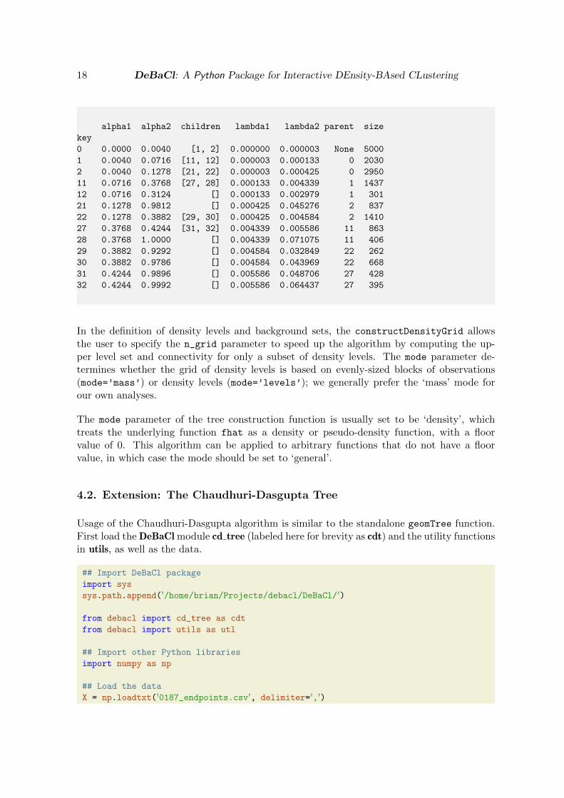
For straightforward cases like this one, we use a single convenience function to do density es-timation, similarity graph definition, level set tree construction, and pruning. In the followingexample, each of these steps will be done separately. Note the print function is overloadedto show a summary of the tree.

## Build the level set tree with the all-in-one function

tree = gtree.geomTree(X, k, gamma, n_grid=None, verbose=False)

print tree

alpha1 alpha2 children lambda1 lambda2 parent size

key

0 0.0000 0.0040 [1, 2] 0.000000 0.000003 None 5000

1 0.0040 0.0716 [11, 12] 0.000003 0.000133 0 2030

2 0.0040 0.1278 [21, 22] 0.000003 0.000425 0 2950

11 0.0716 0.3768 [27, 28] 0.000133 0.004339 1 1437

12 0.0716 0.3124 [] 0.000133 0.002979 1 301

21 0.1278 0.9812 [] 0.000425 0.045276 2 837

22 0.1278 0.3882 [29, 30] 0.000425 0.004584 2 1410

27 0.3768 0.4244 [31, 32] 0.004339 0.005586 11 863

28 0.3768 1.0000 [] 0.004339 0.071075 11 406

29 0.3882 0.9292 [] 0.004584 0.032849 22 262

30 0.3882 0.9786 [] 0.004584 0.043969 22 668

31 0.4244 0.9896 [] 0.005586 0.048706 27 428

32 0.4244 0.9992 [] 0.005586 0.064437 27 395

The next step is to assign cluster labels to a set of foreground data points with the functionGeomTree.getClusterLabels. The desired labeling method is specified with the method

argument. When the correct number of clusters K is known, the first-k option retrieves thefirst K disjoint clusters that appear when λ is increased from 0. Alternately, the upper-set

option cuts the tree at a single level, which is useful if the goal is to include or exclude a certainfraction of the data from the upper level set. Here we use this function with α set to 0.05,which removes the 5% of the observations with the lowest estimated density (i.e. outliers) andclusters the remainder. Finally, the all-mode option returns a foreground cluster for eachleaf of the level set tree, which avoids the need to specify either K, λ, or α.

Additional arguments for each method are specified by keyword argument; thegetClusterLabels method parses them intelligently. For all of the labeling methods the


function returns two objects. The first is an m× 2 matrix, where m is the number of pointsin the foreground set. The first column is the index of an observation in the full data matrix,and the second column is the cluster label. The second object is a list of the tree nodes thatare foreground clusters. This is useful for coloring level set tree nodes to match observationsplotted in feature space.

uc_k, nodes_k = tree.getClusterLabels(method='first-k', k=3)

uc_lambda, nodes_lambda = tree.getClusterLabels(method='upper-set', threshold=0.05,

scale='lambda')uc_mode, nodes_mode = tree.getClusterLabels(method='all-mode')

The GeomTree.plot method draws the level set tree dendrogram, with the vertical scalecontrolled by the form parameter. See Section 3.2 for more detail. The three plot forms areshown in Figure 4, foreground clusters are derived from first-k clustering with K set to 3. theplotForeground function from the DeBaCl utils module is used to match the node colors inthe dendrogram to the clusters in feature space. Note that the plot function returns a tuplewith several objects, but only the first is useful for most applications.

## Plot the level set tree with three different vertical scales, colored by the

first-K clustering

fig = tree.plot(form='lambda', width='mass', color_nodes=nodes_k)[0]

fig.savefig('../figures/endpt_tree_lambda.png')

fig = tree.plot(form='alpha', width='mass', color_nodes=nodes_k)[0]

fig.savefig('../figures/endpt_tree_alpha.png')

fig = tree.plot(form='kappa', width='mass', color_nodes=nodes_k)[0]

fig.savefig('../figures/endpt_tree_kappa.png')

## Plot the foreground points from the first-K labeling

fig, ax = utl.plotForeground(X, uc_k, fg_alpha=0.6, bg_alpha=0.4, edge_alpha=0.3, s

=22)

ax.elev = 14; ax.azim=160 # adjust the camera angle

fig.savefig('../figures/endpt_firstK_fg.png', bbox_inches='tight')

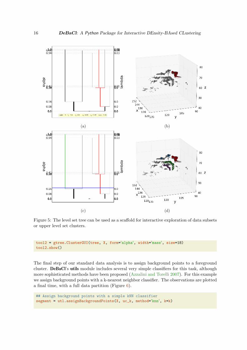
A level set tree plot is also useful as a scaffold for interactive exploration of spatially coherentsubsets of data, either by selecting individual nodes of the tree or by retreiving high-densityclusters at a selected density or mass level. These tools are particularly useful for exploringclustering features at multiple data resolutions. In Figure 5, for example, there are twodominant clusters, but each one has highly salient clustering behavior at higher resolutions.The interactive tools allow for exploration of the parent-child relationships between theseclusters.

tool1 = gtree.ComponentGUI(tree, X, form='alpha', output=['scatter'], size=18, width=

'mass')tool1.show()


(a) Fiber endpoint data, colored by first-Kforeground cluster (b) Lambda scale

(c) Alpha scale (d) Kappa scale

Figure 4: First-k clustering results with different vertical scales and the clusters in featurespace.


(a) (b)

(c) (d)

Figure 5: The level set tree can be used as a scaffold for interactive exploration of data subsetsor upper level set clusters.

tool2 = gtree.ClusterGUI(tree, X, form='alpha', width='mass', size=18)

tool2.show()

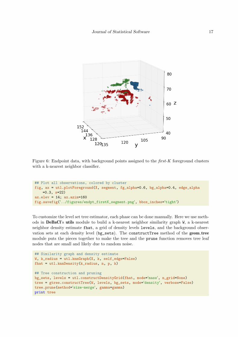
The final step of our standard data analysis is to assign background points to a foregroundcluster. DeBaCl’s utils module includes several very simple classifiers for this task, althoughmore sophisticated methods have been proposed (Azzalini and Torelli 2007). For this examplewe assign background points with a k-nearest neighbor classifier. The observations are plotteda final time, with a full data partition (Figure 6).

## Assign background points with a simple kNN classifier

segment = utl.assignBackgroundPoints(X, uc_k, method='knn', k=k)


Figure 6: Endpoint data, with background points assigned to the first-K foreground clusterswith a k-nearest neighbor classifier.

## Plot all observations, colored by cluster

fig, ax = utl.plotForeground(X, segment, fg_alpha=0.6, bg_alpha=0.4, edge_alpha

=0.3, s=22)

ax.elev = 14; ax.azim=160

fig.savefig('../figures/endpt_firstK_segment.png', bbox_inches='tight')

To customize the level set tree estimator, each phase can be done manually. Here we use meth-ods in DeBaCl’s utils module to build a k-nearest neighbor similarity graph W, a k-nearestneighbor density estimate fhat, a grid of density levels levels, and the background obser-vation sets at each density level (bg_sets). The constructTree method of the geom treemodule puts the pieces together to make the tree and the prune function removes tree leafnodes that are small and likely due to random noise.

## Similarity graph and density estimate

W, k_radius = utl.knnGraph(X, k, self_edge=False)

fhat = utl.knnDensity(k_radius, n, p, k)

## Tree construction and pruning

bg_sets, levels = utl.constructDensityGrid(fhat, mode='mass', n_grid=None)

tree = gtree.constructTree(W, levels, bg_sets, mode='density', verbose=False)

tree.prune(method='size-merge', gamma=gamma)

print tree



key

0 0.0000 0.0040 [1, 2] 0.000000 0.000003 None 5000

1 0.0040 0.0716 [11, 12] 0.000003 0.000133 0 2030

2 0.0040 0.1278 [21, 22] 0.000003 0.000425 0 2950

11 0.0716 0.3768 [27, 28] 0.000133 0.004339 1 1437

12 0.0716 0.3124 [] 0.000133 0.002979 1 301

21 0.1278 0.9812 [] 0.000425 0.045276 2 837

22 0.1278 0.3882 [29, 30] 0.000425 0.004584 2 1410

27 0.3768 0.4244 [31, 32] 0.004339 0.005586 11 863

28 0.3768 1.0000 [] 0.004339 0.071075 11 406

29 0.3882 0.9292 [] 0.004584 0.032849 22 262

30 0.3882 0.9786 [] 0.004584 0.043969 22 668

31 0.4244 0.9896 [] 0.005586 0.048706 27 428

32 0.4244 0.9992 [] 0.005586 0.064437 27 395

In the definition of density levels and background sets, the constructDensityGrid allowsthe user to specify the n_grid parameter to speed up the algorithm by computing the up-per level set and connectivity for only a subset of density levels. The mode parameter de-termines whether the grid of density levels is based on evenly-sized blocks of observations(mode=’mass’) or density levels (mode=’levels’); we generally prefer the ‘mass’ mode forour own analyses.

The mode parameter of the tree construction function is usually set to be ‘density’, whichtreats the underlying function fhat as a density or pseudo-density function, with a floorvalue of 0. This algorithm can be applied to arbitrary functions that do not have a floorvalue, in which case the mode should be set to ‘general’.

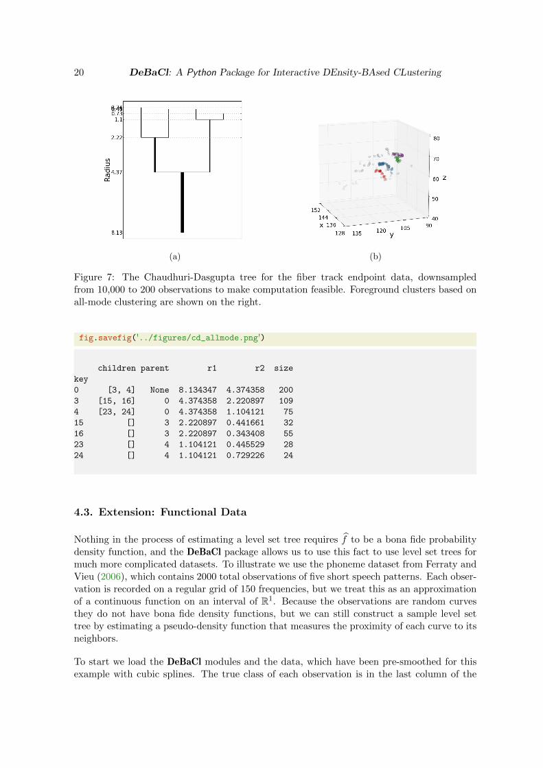
4.2. Extension: The Chaudhuri-Dasgupta Tree

Usage of the Chaudhuri-Dasgupta algorithm is similar to the standalone geomTree function.First load the DeBaCl module cd tree (labeled here for brevity as cdt) and the utility functionsin utils, as well as the data.


import sys


from debacl import cd_tree as cdt



import numpy as np

## Load the data

X = np.loadtxt('0187_endpoints.csv', delimiter=',')


n, p = X.shape

Because the straightforward implementation of the Chaudhuri-Dasgupta algorithm is ex-tremely slow, we use a random subset of only 200 observations (out of the total of 10,000).The smoothing parameter is set to be 2.5% of n, or 5. The pruning parameter is 5% of n, or10. The pruning parameter is slightly less important for the Chaudhuri-Dasgupta algorithm.

## Downsample

n_samp = 200

ix = np.random.choice(range(n), size=n_samp, replace=False)

X = X[ix, :]

n, p = X.shape

## Set level set tree parameters

p_k = 0.025

p_gamma = 0.05

k = int(p_k * n)




figsize=(8,8))

The straightforward implementation of the Chaudhuri-Dasgupta algorithm starts with a com-plete graph and removes one edge a time, which is extremely slow. The start parameter ofthe cdTree function allows for shortcuts. These are approximations to the method, but arenecessary to make the algorithm practical. Currently, the only implemented shortcut is tostart with a k-nearest neighbor graph.

## Construct the level set tree estimate

tree = cdt.cdTree(X, k, alpha=1.4, start='knn', verbose=False)


As with the geometric tree, we can print a summary of the tree, plot the tree, retrieveforeground cluster labels, and plot the foreground clusters. This is illustrated below for the‘all-mode’ labeling method.

## Print/make output

print tree

fig = tree.plot()

fig.savefig('../figures/cd_tree.png')

uc, nodes = tree.getClusterLabels(method='all-mode')

fig, ax = utl.plotForeground(X, uc, fg_alpha=0.6, bg_alpha=0.4, edge_alpha=0.3, s

=60)

ax.elev = 14; ax.azim=160


(a) (b)

Figure 7: The Chaudhuri-Dasgupta tree for the fiber track endpoint data, downsampledfrom 10,000 to 200 observations to make computation feasible. Foreground clusters based onall-mode clustering are shown on the right.

fig.savefig('../figures/cd_allmode.png')

children parent r1 r2 size

key

0 [3, 4] None 8.134347 4.374358 200

3 [15, 16] 0 4.374358 2.220897 109

4 [23, 24] 0 4.374358 1.104121 75

15 [] 3 2.220897 0.441661 32

16 [] 3 2.220897 0.343408 55

23 [] 4 1.104121 0.445529 28

24 [] 4 1.104121 0.729226 24

4.3. Extension: Functional Data

Nothing in the process of estimating a level set tree requires f to be a bona fide probabilitydensity function, and the DeBaCl package allows us to use this fact to use level set trees formuch more complicated datasets. To illustrate we use the phoneme dataset from Ferraty andVieu (2006), which contains 2000 total observations of five short speech patterns. Each obser-vation is recorded on a regular grid of 150 frequencies, but we treat this as an approximationof a continuous function on an interval of R1. Because the observations are random curvesthey do not have bona fide density functions, but we can still construct a sample level settree by estimating a pseudo-density function that measures the proximity of each curve to itsneighbors.

To start we load the DeBaCl modules and the data, which have been pre-smoothed for thisexample with cubic splines. The true class of each observation is in the last column of the


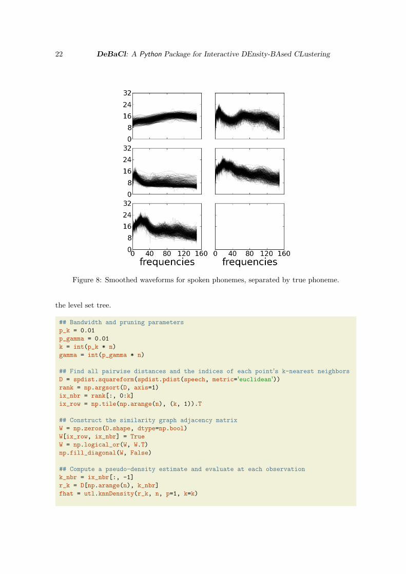
raw data object. The curves for each phoneme are shown in Figure 8.


import sys


from debacl import geom_tree as gtree



import numpy as np

import scipy.spatial.distance as spdist

import matplotlib.pyplot as plt



figsize=(8,8))

## Load data

speech = np.loadtxt('smooth_phoneme.csv', delimiter=',')phoneme = speech[:, -1].astype(np.int)

speech = speech[:, :-1]

n, p = speech.shape

## Plot the curves, separated by true phoneme

fig, ax = plt.subplots(3, 2, sharex=True, sharey=True)

ax = ax.flatten()

ax[-2].set_xlabel('frequencies')ax[-1].set_xlabel('frequencies')

for g in np.unique(phoneme):

ix = np.where(phoneme == g)[0]

for j in ix:

ax[g].plot(speech[j, :], c='black', alpha=0.15)

fig.savefig('../figures/phoneme_data.png')

For functional data we need to define a distance function, precluding the use of the conveniencemethod GeomTree.geomTree or even the utility function utils.knnGraph. First the bandwithand tree pruning parameters are set to be 0.01n. In the second step all pairwise distances arecomputed in order to find the k-nearest neighbors for each observation. For simplicity we useEuclidean distance between a pair of curves (which happens to work well in this example), butthis is not generally optimal. Next, the adjacency matrix for a k-nearest neighbor graph isconstructed, which is no different than the finite-dimensional case. Finally the pseudo-densityestimator is built by using the finite-dimenisonal k-nearest neighbor density estimator withthe dimension set (incorrectly) to 1. This function does not integrate to 1, but the functioninduces an ordering on the observations (from smallest to largest k-neighbor radius) that isinvariant to the dimension. This ordering is all that is needed for the final step of building


Figure 8: Smoothed waveforms for spoken phonemes, separated by true phoneme.

the level set tree.

## Bandwidth and pruning parameters

p_k = 0.01

p_gamma = 0.01

k = int(p_k * n)


## Find all pairwise distances and the indices of each point's k-nearest neighbors

D = spdist.squareform(spdist.pdist(speech, metric='euclidean'))rank = np.argsort(D, axis=1)

ix_nbr = rank[:, 0:k]

ix_row = np.tile(np.arange(n), (k, 1)).T

## Construct the similarity graph adjacency matrix

W = np.zeros(D.shape, dtype=np.bool)

W[ix_row, ix_nbr] = True

W = np.logical_or(W, W.T)

np.fill_diagonal(W, False)

## Compute a pseudo-density estimate and evaluate at each observation

k_nbr = ix_nbr[:, -1]

r_k = D[np.arange(n), k_nbr]

fhat = utl.knnDensity(r_k, n, p=1, k=k)


## Build the level set tree

bg_sets, levels = utl.constructDensityGrid(fhat, mode='mass', n_grid=None)

tree = gtree.constructTree(W, levels, bg_sets, mode='density', verbose=False)


print tree


key

0 0.0000 0.2660 [1, 2] 0.000000 0.000261 None 2000

1 0.2660 0.3435 [3, 4] 0.000261 0.000275 0 1125

2 0.2660 1.0000 [] 0.000261 0.000938 0 343

3 0.3435 0.4905 [5, 6] 0.000275 0.000307 1 565

4 0.3435 0.7705 [] 0.000275 0.000426 1 413

5 0.4905 0.9920 [] 0.000307 0.000808 3 391

6 0.4905 0.7110 [] 0.000307 0.000382 3 85

Once the level set tree is constructed we can plot it and retrieve cluster labels as with finite-dimensional data. In this case we choose the all-mode cluster labeling which produces fourclusters. The utility function utils.plotForeground is currently designed to work only withtwo- or three-dimensional data, so plotting the foreground clusters must be done manuallyfor functional data. The clusters from this procedure match the true groups quite well, atleast in a qualitative sense.

## Retrieve cluster labels

uc, nodes = tree.getClusterLabels(method='all-mode')

## Level set tree plot

fig = tree.plot(form='alpha', width='mass', color_nodes=nodes)[0]

fig.savefig('../figures/phoneme_tree.png')

## Plot the curves, colored by foreground cluster

palette = utl.Palette()

fig, ax = plt.subplots()

ax.set_xlabel("frequency index")

for c in np.unique(uc[:,1]):

ix = np.where(uc[:,1] == c)[0]

ix_clust = uc[ix, 0]

for i in ix_clust:

ax.plot(speech[i,:], c=np.append(palette.colorset[c], 0.25))

fig.savefig('../figures/phoneme_allMode.png')

5. Conclusion


Figure 9: All-mode foreground clusters for the smoothed phoneme data.

The Python package DeBaCl for hierarchical density-based clustering provides a highly usableimplementation of level set tree estimation and clustering. It improves on existing softwarethrough computational efficiency and a high-degree of modularity and customization. Namely,DeBaCl:

• offers the first known implementation of the theoretically well-supported Chaudhuri-Dasgupta level set tree algorithm;

• allows for very general data ordering functions, which are typically probability densityestimates but could also be pseudo-density estimates for infinite-dimensional functionaldata or even arbitrary functions;

• accepts any similarity graph, density estimator, pruning function, cluster labelingscheme, and background point assignment classifier;

• includes the all-mode cluster labeling scheme, which does not require an a priori choiceof the number of clusters;

• incorporates the λ, α, and κ vertical scales for plotting level set trees, as well as otherplotting tweaks to make level set tree plots more interpretable and usable;

• and finally, includes interactive GUI tools for selecting coherent data subsets or high-density clusters based on the level set tree.


The DeBaCl package and user manual is available at https://github.com/CoAxLab/DeBaCl.The project remains under active development; the focus for the next version will be on im-provements in computational efficiency, particularly for the Chaudhuri-Dasgupta algorithm.

Acknowledgments

This research was sponsored by the Army Research Laboratory and was accomplished underCooperative Agreement Number W911NF-10-2-0022. The views and conclusions containedin this document are those of the authors and should not be interpreted as representing theofficial policies, either expressed or implies, of the Army Research Laboratory or the U.S.Government. The U.S. Government is authorized to reproduce and distribute reprints for theGovernment purposes notwithstanding any copyright notation herein. This research was alsosupported by NSF CAREER grant DMS 114967.

References

Azzalini A, Menardi G (2012). “Clustering via Nonparametric Density Estimation : theR Package pdfCluster.” Technical Report 1, University of Padua. URL http://cran.

r-project.org/web/packages/pdfCluster/index.html.

Azzalini A, Torelli N (2007). “Clustering via nonparametric density estimation.” Statisticsand Computing, 17(1), 71–80. ISSN 0960-3174. doi:10.1007/s11222-006-9010-y. URLhttp://www.springerlink.com/index/10.1007/s11222-006-9010-y.

Balakrishnan BS, Narayanan S, Rinaldo A, Singh A, Wasserman L (2013). “Cluster Trees onManifolds.” arXiv [stat.ML], pp. 1–28. arXiv:1307.6515v1.

Billingsley P (2012). Probability and Measure. Wiley. ISBN 978-1118122372.

Chaudhuri K, Dasgupta S (2010). “Rates of convergence for the cluster tree.” In Advances inNeural Information Processing Systems 23, pp. 343–351. Vancouver, BC.

Csardi G, Nepusz T (2006). “The igraph Software Package for Complex Network Research.”InterJournal, 1695(38).

Ester M, Kriegel Hp, Xu X (1996). “A Density-Based Algorithm for Discovering Clustersin Large Spatial Databases with Noise.” In Knowledge Discovery and Data Mining, pp.226–231.

Ferraty F, Vieu P (2006). Nonparametric Functional Data Analysis. Springer. ISBN9780387303697.

Hartigan J (1975). Clustering Algorithms. John Wiley & Sons. ISBN 978-0471356455.

Hartigan JA (1981). “Consistency of Single Linkage for High-Density Clusters.” Journal ofthe American Statistical Association, 76(374), 388–394.

https://github.com/CoAxLab/DeBaCl

http://cran.r-project.org/web/packages/pdfCluster/index.html

http://cran.r-project.org/web/packages/pdfCluster/index.html

http://dx.doi.org/10.1007/s11222-006-9010-y

http://www.springerlink.com/index/10.1007/s11222-006-9010-y

arXiv:1307.6515v1


Hennig C (2013). “fpc: Flexible procedures for clustering.” URL http://cran.r-project.

org/package=fpc.

Hunter JD (2007). “Matplotlib: A 2D Graphics Environment.” Computing in Science &Engineering, 9(3), 90–95. URL http://matplotlib.org/.

Jones E, Oliphant T, Peterson P (2001). “SciPy: Open Source Scientific Tools for Python.”URL http://www.scipy.org/.

Klemela J (2004). “Visualization of Multivariate Density Estimates With Level Set Trees.”Journal of Computational and Graphical Statistics, 13(3), 599–620. ISSN 1061-8600.doi:10.1198/106186004X2642. URL http://www.tandfonline.com/doi/abs/10.1198/

106186004X2642.

Klemela J (2005). “Algorithms for Manipulation of Level Sets of Nonparametric DensityEstimates.” Computational Statistics, 20(2), 349–368. doi:10.1007/BF02789708.

Kpotufe S, Luxburg UV (2011). “Pruning nearest neighbor cluster trees.” Proceedings of the28th International Conference on Machine Learning, 105, 225–232.

Lei J, Robins J, Wasserman L (2013). “Distribution-Free Prediction Sets.” Journalof the American Statistical Association, 108(501), 278–287. ISSN 0162-1459. doi:

10.1080/01621459.2012.751873.

Lloyd S (1982). “Least squares quantization in PCM.” IEEE Transactions on InformationTheory, 28(2), 129–137. ISSN 0018-9448. doi:10.1109/TIT.1982.1056489.

MacQueen J (1967). “Some Methods for Classification and And Analysis of MultivariateObservations.” Proceedings of the 5th Berkeley Symposium on Mathematical Statistics andProbability, 1, 281–297.

Maier M, Hein M, von Luxburg U (2009). “Optimal construction of k-nearest-neighbor graphsfor identifying noisy clusters.” Theoretical Computer Science, 410(19), 1749–1764. ISSN03043975. doi:10.1016/j.tcs.2009.01.009.

Menardi G, Azzalini A (2013). “An Advancement in Clustering via Nonparametric Density Es-timation.” Statistics and Computing. ISSN 0960-3174. doi:10.1007/s11222-013-9400-x.URL http://link.springer.com/10.1007/s11222-013-9400-x.

Pedregosa F, Varoquaux G, Gramfort A, Michel V, Thirion B, Grisel O, Blondel M, Pretten-hofer P, Weiss R, Dubourg V, Vanderplas J, Passos A, Cournapeau D, Brucher M, PerrotM, Duchesnay E (2011). “Scikit-learn : Machine Learning in Python.” Journal of MachineLearning Research, 12, 2825–2830.

Polonik W (1995). “Measuring Mass Concentrations and Estimating Density Contour Clusters- An Excess Mass Approach.” The Annals of Statistics, 23(3), 855–881.

Rinaldo A, Singh A, Nugent R, Wasserman L (2012). “Stability of Density-Based Clustering.”Journal of Machine Learning Research, 13, 905–948. arXiv:1011.2771v1.

Rinaldo A, Wasserman L (2010). “Generalized density clustering.” The Annals of Statistics,38(5), 2678–2722. ISSN 0090-5364. doi:10.1214/10-AOS797. arXiv:0907.3454v3, URLhttp://projecteuclid.org/euclid.aos/1278861457.

http://cran.r-project.org/package=fpc

http://cran.r-project.org/package=fpc

http://matplotlib.org/

http://www.scipy.org/

http://dx.doi.org/10.1198/106186004X2642

http://www.tandfonline.com/doi/abs/10.1198/106186004X2642

http://www.tandfonline.com/doi/abs/10.1198/106186004X2642

http://dx.doi.org/10.1007/BF02789708

http://dx.doi.org/10.1080/01621459.2012.751873

http://dx.doi.org/10.1080/01621459.2012.751873

http://dx.doi.org/10.1109/TIT.1982.1056489

http://dx.doi.org/10.1016/j.tcs.2009.01.009

http://dx.doi.org/10.1007/s11222-013-9400-x

http://link.springer.com/10.1007/s11222-013-9400-x

arXiv:1011.2771v1

http://dx.doi.org/10.1214/10-AOS797

arXiv:0907.3454v3

http://projecteuclid.org/euclid.aos/1278861457


Shi J, Malik J (2000). “Normalized Cuts and Image Segmentation.” IEEE Transactions onPattern Analysis and Machine Intelligence, 22(8), 888–905.

Sriperumbudur BK, Steinwart I (2012). “Consistency and Rates for Clustering with DB-SCAN.” JMLR Workshop and Conference Proceedings, 22, 1090–1098.

Steinwart I (2011). “Adaptive Density Level Set Clustering.” Journal of Machine LearningResearch: Workshop and Conference Proceedings - 24th Annual Conference on LearningTheory, pp. 1–35.

Stuetzle W, Nugent R (2010). “A Generalized Single Linkage Method for Estimating theCluster Tree of a Density.” Journal of Computational and Graphical Statistics, 19(2), 397–418. ISSN 1061-8600. doi:10.1198/jcgs.2009.07049. URL http://www.tandfonline.

com/doi/abs/10.1198/jcgs.2009.07049.

Wishart D (1969). “Mode analysis: a generalization of nearest neighbor which reduces chainingeffects.” In AJ Cole (ed.), Proceedings of the Colloquium on Numerical Taxonomy held inthe University of St. Andrews, pp. 282–308.

Wong A, Lane T (1983). “A kth Nearest Neighbour Clustering Procedure.” Journal of theRoyal Statistical Society: Series B, 45(3), 362–368.

Affiliation:

Brian P. KentDepartment of StatisticsCarnegie Mellon UniversityBaker Hall 132Pittsburgh, PA 15213E-mail: [email protected]: http://www.brianpkent.com

Alessandro RinaldoDepartment of StatisticsCarnegie Mellon UniversityBaker Hall 132Pittsburgh, PA 15213E-mail: [email protected]: http://www.stat.cmu.edu/~arinaldo/

http://dx.doi.org/10.1198/jcgs.2009.07049

http://www.tandfonline.com/doi/abs/10.1198/jcgs.2009.07049

http://www.tandfonline.com/doi/abs/10.1198/jcgs.2009.07049

mailto:[email protected]

http://www.brianpkent.com


http://www.stat.cmu.edu/~arinaldo/


Timothy VerstynenDepartment of Psychology & Center for the Neural Basis of CognitionCarnegie Mellon UniversityBaker Hall 340UPittsburgh, PA 15213E-mail: [email protected]: http://www.psy.cmu.edu/~coaxlab/

Journal of Statistical Software http://www.jstatsoft.org/

published by the American Statistical Association http://www.amstat.org/

Volume VV, Issue II Submitted: yyyy-mm-ddMMMMMM YYYY Accepted: yyyy-mm-dd


http://www.psy.cmu.edu/~coaxlab/

http://www.jstatsoft.org/

http://www.amstat.org/

debacl: a python package for interactive density … · 2 debacl: a python package for interactive...

Documents