dealing with trends in dsge models
TRANSCRIPT
Dealing with trends in DSGE modelsESRI Conference, Tokyo, November 14, 2008
Michel Juillard (Bank of France and CEPREMAP)
Introduction
I Traditionally, separation betweenI short term, fluctuation analysisI long term, growth models
I In practice,I write business cycle model without trendsI estimate on detrended data

Alternative procedure
I include growth in the model, i.e. neo–classical growthmodel,
I estimate on original data, in level or in growth rates.
Difficulties:I solution methods using a perturbation approach imply a
local approximation around a deterministic steady state.I estimating a model with stochastic trends and data in level
require a special initialization of the Kalman filter.
Solutions:I local approximations can only be used with balanced
growth modelsI for estimation in level use a diffuse initialization for the
Kalman filter (Durbin and Koopman)
Outline
I Stationarizing balanced growth modelsI Diffuse Kalman filter

Balanced growth
I In absence of shocks, variables grow at a constant ratesI Real production variables grow at the rate of technical
progressI Employment grows at the rate of demographic growthI Nominal variables grow like money supplyI Prices grow like the ratio of money supply over technical
progressI Hours, interest rates, inflation are stationary (unless
inflation target follows a stochastic trend)I Different sectors may have different rates of technical
change (Edge, Laubach, Williams; Ireland and Schuh)

Stationarizing the model
I local approximation (perturbation approach) requires aconstant deterministic steady state
I stationarized variables are divided by their correspondingtrend
I balanced growth models are invariant to this change ofvariable
I the trends themselves (deterministic or stochastic) can bemodeled as log–linear processes
log dt = log dt−1 + g
log st = log st−1 + g + et
I (log–)linear processes don’t need to be locallyapproximated!
I this procedure is equivalent to take a local approximationaround the balanced growth path.
Standard CIA model
Nason and Cogley (1994), Schorfheide (2000)I Three agents:
I householdsI firmsI financial intermediaries
I Decisions are made after the current period surprisechange in money growth and technology.

Firm
The firm chooses desired capital, Kt , labour demand, Nt ,dividends Ft and loans Lt
max{Kt ,Nt ,Ft}
∞
t=0
E0
[∞∑
t=0
βt Ft
Ct+1Pt+1
]
s.t.
Ft ≤ Lt + Pt Yt − Kt + (1 − δ)Kt−1 − Wt Nt − RF ,tLt
Wt Nt ≤ Lt
Yt = K α
t−1 (At Nt)1−α
where Yt is output, At , technical change index, Pt , the priceindex, Wt , the wage rate, and RF ,t , the gross interest rate onloans.

Financial Intermediary
The following maximisation problem:
max{Bt ,Lt ,Dt}
∞
t=0
E0
[∞∑
t=0
βt Bt
Ct+1Pt+1
]
s.t.
Bt = Dt + RF ,tLt − RH,tDt − Lt + Mt − Mt−1
Lt ≤ Mt − Mt−1 + Dt
where Bt is dividends from the financial intermediaries, Dt , thedeposits, and RH,t is the gross deposit interest rate.

Household
The household chooses consumption Ct , hours worked Ht , and(non-negative) deposits Dt so that
max{Ct ,Ht ,Mt ,Dt}
∞
t=0
E0
[∞∑
t=0
βt [(1 − ψ) log Ct + ψ log(1 − Ht)]
]
s.t.
PtCt ≤ Mt−1 − Dt + WtHt
Dt ≥ 0
Mt = Mt−1 − Dt + WtHt − PtCt + RH,tDt + Ft + Bt

Market clearing conditions
I Labor marketHt = Nt
I Money marketPtCt = Mt
I Goods market
Ct + (Kt − (1 − δ)Kt−1) = (1 + eGt)Kαt−1(AtNt)
1−α

Shock processes
Technology:
gAt =At
At−1
log gAt = γ + εAt
Demand shock:
eGt
Money:
gMt =Mt
Mt−1
log gMt = (1 − ρ) log gM? + ρ log gMt−1 + εM t

Optimality conditions
Et
{Pt
Ct+1Pt+1
}= βEt
{Pt+1αK α−1
t (At+1Nt+1)1−α + 1 − δ
Ct+2Pt+2
}
ψ
1 − ψ
CtPt
1 − Nt= Wt
1CtPt
= βEt
{Rt
Ct+1Pt+1
}
Rt =Pt(1 − α)K α
t−1A1−αt N−α
t
Wt

Other equilibrium conditions
Wt =Lt
Nt
Lt = Mt − Mt−1 + Dt
PtCt = Mt
Ct + (Kt − (1 − δ)Kt−1) = (1 − eGt)Kαt−1(AtNt)
1−α
gAt =At
At−1
log gAt = γ + εAt
gM t =Mt
Mt−1
log gM t = (1 − ρ) log gM? + ρ log gM t−1 + εM t

Stationarized model
In order for a local approximation to make sense, the modelvariables must fluctuate in the neighborhood of the steadystate. It is therefor necessary to stationarize the model, beforecomputing the local approximation of the solution.
I Kt , Ct , are detrended by the productivity At ,
I Pt is detrended by Mt−1/At
I Wt , Lt , and Dt are detrended by Mt−1.I Rt and Nt are stationary

First-order conditions
Euler equation:
Et
{Pt
Mt−1At
Ct+1At+1Pt+1Mt
At+1
}
= βEt
{Pt+1
Mt
At+1
α(
KtAt
)α−1(At+1Nt+1)
1−α + 1 − δ
Ct+2At+2Pt+2Mt+1At+2
}
after simplification
Et
{Pt
Ct+1Pt+1gMt
}= βEt
{Pt+1
αgA−αt+1K α−1
t N1−αt+1 + 1−δ
gAt+1
Ct+2Pt+2gM t+1
}

First-order conditions (continued)Firm’s borrowing constraint:
WtMt−1 =LtMt−1
Nt
after simplification
Wt =Lt
Nt
Intertemporal labor market optimality condition:
ψ
1 − ψ
CtAt PtMt−1
At
1 − Nt= WtMt−1
after simplification
ψ
1 − ψ
Ct Pt
1 − Nt= Wt

First order conditions (continued)Equilibrium interest rate:
Rt =(1 − α)Pt
Mt−1At
(Kt−1At−1
)α−1(AtNt)
−α
WtMt−1
after simplification
Rt =(1 − α)PtgA
−αt K α−1
t−1 N−αt
Wt
Credit market optimality condition:
1
CtAt PtMt−1
At
= βEt
{Rt
Ct+1At+1Pt+1Mt
At+1
}
after simplification
1
Ct Pt
= βEt
{Rt
gM tCt+1Pt+1
}

Other equilibrium conditions
Wt =Lt
Nt
Lt = gMt − 1 + Dt
Pt Ct = gMt
Ct + Kt − (1 − δ)Kt−1
gAt= (1 − eGt)
(Kt−1
gAt
)α
N1−αt
log gAt = γ + εAt
log gMt = (1 − ρ) log gM? + ρ log gMt−1 + εM t
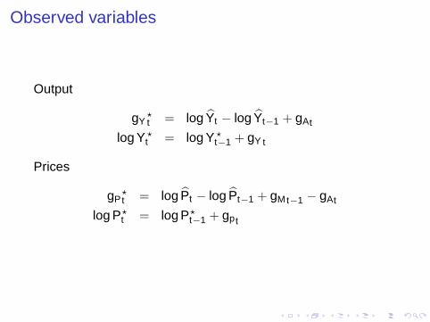
Observed variables
Output
gY?t = log Yt − log Yt−1 + gAt
log Y ?t = log Y ?
t−1 + gY t
Prices
gP?t = log Pt − log Pt−1 + gMt−1 − gAt
log P?t = log P?
t−1 + gpt
Difference with VAR analysis
I If the true model is a Vector Error Correction Model,estimating a VAR in first difference implies amispecificaton.
I This isn’t the case with structural modeling, because thevariables in level are among unobserved components.

Estimation strategy
I After (log–)linearization around the deterministic steadystate, the linear rational expectation model needs to besolved (AIM, Kind and Watson, Klein, Sims)
I The model can then be written in state space formI It is an unobserved component modelI Its likelihood is computed via the Kalman filterI These steps are common to Maximum Likelihood
estimation or a Bayesian approach

State space representation (I)
After solution of a first order approximation of a DSGE model,we obtain a linear dynamic model of the form
yt = y + gy yst−1 + guut
the vector yst−1 contains the endogenous state variables, the
predetermined variables among yt , with as many lags asrequired by the dynamic of the model.
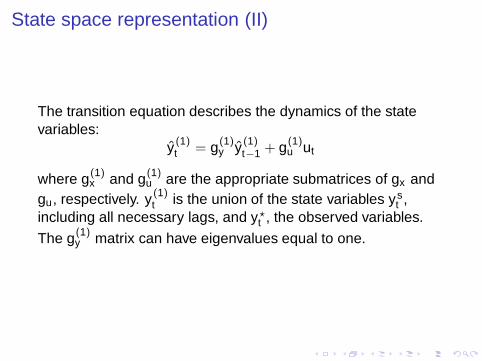
State space representation (II)
The transition equation describes the dynamics of the statevariables:
y (1)t = g(1)
y y (1)t−1 + g(1)
u ut
where g(1)x and g(1)
u are the appropriate submatrices of gx andgu, respectively. y (1)
t is the union of the state variables yst ,
including all necessary lags, and y?t , the observed variables.
The g(1)y matrix can have eigenvalues equal to one.
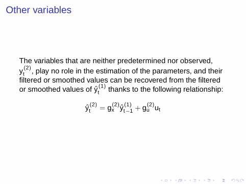
Other variables
The variables that are neither predetermined nor observed,y (2)
t , play no role in the estimation of the parameters, and theirfiltered or smoothed values can be recovered from the filteredor smoothed values of y (1)
t thanks to the following relationship:
y (2)t = g(2)
x y (1)t−1 + g(2)
u ut

Measurement equation
We consider measurement equations of the type
y?t = y + My (1)
t + xt + εt
where M is the selection matrix that recovers y?t out of y (1)
t , xt
is a deterministic component1 and εt is a vector ofmeasurement errors.
1Currently, Dynare only accomodates linear trends

Variances
In addition, we have, the two following covariance matrices:
E(utu′
t
)= Q
E(εtε
′t
)= H

Unit root processes
I find a natural representation in the state space formI the deterministic components of random walk with drift is
better included in the measurement equation

Initialization of the Kalman filter
I stationary variables: unconditional mean and varianceI nonstationary variables: initial point is an additional
parameter of the model (De Jong), arbitrary initial pointand infinite variance (Durbin and Koopman).
I Durbin and Koopman strategy: compute the limit of theKalman filter equations when initial variance tends towardinfinity.
I Problem with cointegrated models.
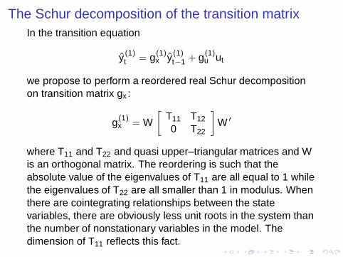
The Schur decomposition of the transition matrixIn the transition equation
y (1)t = g(1)
x y (1)t−1 + g(1)
u ut
we propose to perform a reordered real Schur decompositionon transition matrix gx :
g(1)x = W
[T11 T12
0 T22
]W ′
where T11 and T22 and quasi upper–triangular matrices and Wis an orthogonal matrix. The reordering is such that theabsolute value of the eigenvalues of T11 are all equal to 1 whilethe eigenvalues of T22 are all smaller than 1 in modulus. Whenthere are cointegrating relationships between the statevariables, there are obviously less unit roots in the system thanthe number of nonstationary variables in the model. Thedimension of T11 reflects this fact.
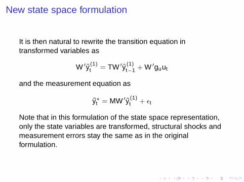
New state space formulation
It is then natural to rewrite the transition equation intransformed variables as
W ′y (1)t = TW ′y (1)
t−1 + W ′guut
and the measurement equation as
y?t = MW ′y (1)
t + εt
Note that in this formulation of the state space representation,only the state variables are transformed, structural shocks andmeasurement errors stay the same as in the originalformulation.

New notations
In what follows, we write the state space model as
yt = Zat + εt
at = Tat−1 + Rηt
E(εtε
′t
)= H
E(ηtη
′t
)= Q
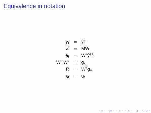
Equivalence in notation
yt = y?t
Z = MW
at = W ′y (1)
WTW ′ = gx
R = W ′gu
ηt = ut
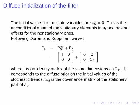
Diffuse initialization of the filter
The initial values for the state variables are a0 = 0. This is theunconditional mean of the stationary elements in at and has noeffects for the nonstationary ones.Following Durbin and Koopman, we set
P0 = P∞0 + P?
0
=
[I 00 0
]+
[0 00 Σa
]
where I is an identity matrix of the same dimensions as T11. Itcorresponds to the diffuse prior on the initial values of thestochastic trends. Σa is the covariance matrix of the stationarypart of at .

Computation of Σa
Σa is the covariance matrix of at with dynamics
at = T12at−1 + Rηt
orΣa = T12ΣaT ′
12 + RQR′
where R is the conforming submatrix of R. As T12 is alreadyquasi upper–triangular, it is only necessary to use part of theusual algorithm for the Lyapunov equation.

The diffuse step
While P∞t is different from zero, the filter (and smoother) is in a
diffuse step. When t > d , the procedure falls back on standardrecursions.At t = 0
E(a1|0
)= P1|0 = P∞
1|0 + P?1|0
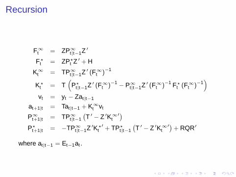
Recursion
F∞t = ZP∞
t|t−1Z ′
F ?
t = ZP?
t Z ′ + H
K∞t = TP∞
t|t−1Z ′ (F∞t )−1
K ?
t = T(
P?
t|t−1Z ′ (F∞t )
−1− P∞
t|t−1Z ′ (F∞t )
−1 F ?
t (F∞t )
−1)
vt = yt − Zat|t−1
at+1|t = Tat|t−1 + K∞t vt
P∞t+1|t = TP∞
t|t−1
(T ′ − Z ′K∞
t′)
P?
t+1|t = −TP∞t|t−1Z ′K ?
t′ + TP?
t|t−1
(T ′ − Z ′K∞
t′)+ RQR′
where at|t−1 = Et−1at .

Log–likelihood
The log–likelihood is given by
−nT2
ln 2π −12
T∑
t=1
ln |Ft | −12
T∑
t=1
v ′t F
−1t vt

Conclusion
I It is possible to specify growth trends in business cycle anddeal with them in a model consistent manner.
I More work is necessary to compare the advantages of thedifferent methods in practice.