de concini–procesi wonderful arrangement models: a discrete
TRANSCRIPT
Combinatorial and Computational GeometryMSRI PublicationsVolume 52, 2005
De Concini–Procesi Wonderful Arrangement
Models: A Discrete Geometer’s Point of View
EVA MARIA FEICHTNER
Abstract. This article outlines the construction of De Concini–Procesi
arrangement models and describes recent progress in understanding their
significance from the algebraic, geometric, and combinatorial point of view.
Throughout the exposition, strong emphasis is given to the combinatorial
and discrete geometric data that lie at the core of the construction.
Contents
1. An Invitation to Arrangement Models 3332. Introducing the Main Character 3343. The Combinatorial Core Data: A Step Beyond Geometry 3424. Returning to Geometry 3485. Adding Arrangement Models to the Geometer’s Toolbox 353Acknowledgments 358References 359
1. An Invitation to Arrangement Models
The complements of coordinate hyperplanes in a real or complex vector space
are easy to understand: The coordinate hyperplanes in Rn dissect the space into
2n open orthants; removing the coordinate hyperplanes from Cn leaves the com-
plex torus (C∗)n. Arbitrary subspace arrangements, i.e., finite families of linear
subspaces, have complements with far more intricate combinatorics in the real
case, and far more intricate topology in the complex case. Arrangement models
improve this complicated situation locally— constructing an arrangement model
means to alter the ambient space so as to preserve the complement and to re-
place the arrangement by a divisor with normal crossings, i.e., a collection of
smooth hypersurfaces which locally intersect like coordinate hyperplanes. Al-
most a decade ago, De Concini and Procesi provided a canonical construction
of arrangement models—wonderful arrangement models — that had significant
impact in various fields of mathematics.
333
334 EVA MARIA FEICHTNER
Why should a discrete geometer be interested in this model construction?
Because there is a wealth of wonderful combinatorial and discrete geometric
structure lying at the heart of the matter. Our aim here is to bring these discrete
pearls to light.
First, combinatorial data plays a descriptive role in various places: The combi-
natorics of the arrangement fully prescribes the model construction and a natural
stratification of the resulting space. We will see details and examples in Section 2.
In fact, the rather coarse combinatorial data reflect enough of the situation so
as to, for instance, determine algebraic-topological invariants of the arrange-
ment models (compare the topological interpretation of the algebra D(L,G) in
Section 4.2).
Secondly, the combinatorial data put forward in the study of arrangement
models invites purely combinatorial generalizations. We discuss such generaliza-
tions in Section 3 and show in Section 4 how this combinatorial generalization
opens unexpected views when related back to geometry.
Finally, in Section 5 we propose arrangement models as a tool for resolving
group actions on manifolds. Again, it is an open eye for discrete core data that
enables the construction.
We have kept the exposition self-contained and illustrated it with many ex-
amples. We invite discrete geometers to discover an algebro-geometric context
in which familiar discrete structures play a key role. We hope that yet many
more bridges will be built between algebraic and discrete geometry— areas that,
despite the differences in terminology, concepts, and methods, share what has
inspired and driven mathematicians for centuries: a passion for geometry.
2. Introducing the Main Character
2.1. Basics on arrangements. We first need to fix some basic terminology, in
particular as it concerns the combinatorial data of an arrangement. We suggest
that the reader, who is not familiar with the setting, reads through the first
part of this Section and compares the notions to the illustrations given for braid
arrangements in Example 2.1.
An arrangement A = {U1, . . . , Un} is a finite family of linear subspaces
in a real or complex vector space V . The topological space most obviously
associated to such an arrangement is its complement in the ambient space,
M(A) := V \S
A.
Having arrangements in real vector spaces in mind, the topology of M(A)
does not look very interesting: the complement is a collection of open polyhedral
cones, and apart from their number there is no significant associated topological
data. In the complex case, however, already a single hyperplane in C1, the origin,
has a nontrivial complement: it is homotopy equivalent to S1, the 1-dimensional
DE CONCINI–PROCESI WONDERFUL ARRANGEMENT MODELS 335
sphere. The complement of two (for instance, coordinate) hyperplanes in C2 is
homotopy equivalent to the torus S1 × S1.
The combinatorial data associated with an arrangement is usually recorded in
the intersection lattice L = L(A), which is the set of intersections of subspaces
in A, partially ordered by reversed inclusion. We adopt terminology from the
theory of partially ordered sets and often denote the unique minimum in L(A)
(corresponding to the empty intersection, i.e., the ambient space V ) by 0 and
the unique maximum of L(A) (the overall intersection of subspaces in A) by 1.
In many situations, the elements of the intersection lattice are labeled by the
codimension of the corresponding intersection. For arrangements of hyperplanes,
this information is recorded in the rank function of the lattice — the codimension
of an intersection X is the number of elements in a maximal chain in the half-
open interval (0, X] in L(A).
As with any poset, we can consider the order complex ∆(L) of the proper part,
L := L \ {0, 1}, of the intersection lattice, i.e., the abstract simplicial complex
formed by the linearly ordered subsets in L,
∆(L) ={X1 < . . . < Xk
∣∣ Xi ∈ L \ {0, 1}}.
The topology of ∆(L) plays a prominent role for describing the topology of ar-
rangement complements. For instance, it is the crucial ingredient for the explicit
description of cohomology groups of M(A) by Goresky and MacPherson [1988,
Part III].
For hyperplane arrangements, the homotopy type of ∆(L) is well known: the
complex is homotopy equivalent to a wedge of spheres of dimension equal to the
codimension of the total intersection of A. The number of spheres can as well be
read from the intersection lattice, it is the absolute value of its Mobius function.
For subspace arrangements however, the barycentric subdivision of any finite
simplicial complex can appear as the order complex of the intersection lattice.
Besides ∆(L), we will often refer to the cone over ∆(L) obtained by extending
the linearly ordered sets in L by the maximal element 1 in L. We will denote
this complex by ∆(L \ {0}) or ∆(L>0).
In order to have a standard example at hand, we briefly discuss braid arrange-
ments. This class of arrangements has figured prominently in many places and
has helped develop lots of arrangement theory over the last decades.
Example 2.1 (Braid arrangements). The arrangement An−1 given by the
hyperplanes
Hij : xi = xj , for 1 ≤ i < j ≤ n,
in real n-dimensional vector space is called the (real) rank n−1 braid arrange-
ment . There is a complex version of this arrangement. It consists of hyperplanes
Hij in Cn given by the same linear equations. We denote the arrangement by
ACn−1. Occasionally, we will use the analogous AR
n−1 if we want to stress the real

336 EVA MARIA FEICHTNER
12
123
13 23
0
23
13
12
123
L(A2) = Π3
∆(Π3 \ {0})
H12 : x1=x2H23 : x2=x3
H13 : x1=x3
A2 ⊆ V
Figure 1. The rank 2 braid arrangement A2, its intersection lattice Π3, and the
order complex ∆(Π3 \ {0}).
setting. In many situations a similar reasoning applies to the real and to the
complex case. To simplify notation, we then use K to denote R or C.
Observe that the diagonal ∆ = {x ∈ Kn | x1 = . . . = xn} is the overall
intersection of hyperplanes in An−1. Without loosing any relevant information on
the topology of the complement, we will often consider An−1 as an arrangement
in complex or real (n−1)-dimensional space V = Kn/∆ ∼={x ∈ Kn |
∑xi = 0
}.
This explains the indexing for braid arrangements, which may appear unusual
at first sight.
The complement M(ARn−1) is a collection of n! polyhedral cones, correspond-
ing to the n! linear orders on n pairwise noncoinciding coordinate entries. The
complement M(ACn−1) is the classical configuration space of the complex plane
F (C, n) ={(x1, . . . , xn) ∈ C
n∣∣ xi 6= xj for i 6= j
}.
This space is the classifying space of the pure braid group, which explains the
occurrence of the term “braid” for this class of arrangements.
As the intersection lattice of the braid arrangement An−1 we recognize the
partition lattice Πn, i.e., the set of set partitions of {1, . . . , n} ordered by reversed
refinement. The correspondence to intersections in the braid arrangement can
be easily described: The blocks of a partition correspond to sets of coordinates
with identical entries, thus to the set of points in the corresponding intersection
of hyperplanes.
The order complex ∆(Πn) is a pure, (n−1)-dimensional complex that is ho-
motopy equivalent to a wedge of (n−1)! spheres of dimension n−1.
In Figure 1 we depict the real rank 2 braid arrangement A2 in V = R3/∆, its
intersection lattice Π3, and the order complex ∆(Π3 \ {0}). We denote partitions
in Π3 by their nontrivial blocks. The complex depicted is a cone over ∆(Π3), a
union of three points, which indeed is the wedge of two 0-dimensional spheres.
DE CONCINI–PROCESI WONDERFUL ARRANGEMENT MODELS 337
D13 D23
H23
H12
H13
D12
YA2= Bl{0}VA2 ⊆ V
D123(0, `)
`
(x, 〈x〉)
(y,H12)
x
y
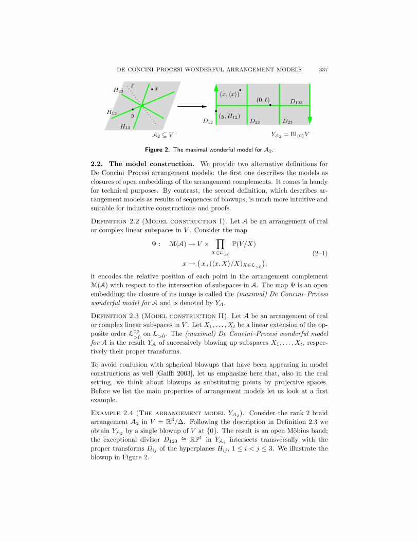
Figure 2. The maximal wonderful model for A2.
2.2. The model construction. We provide two alternative definitions for
De Concini–Procesi arrangement models: the first one describes the models as
closures of open embeddings of the arrangement complements. It comes in handy
for technical purposes. By contrast, the second definition, which describes ar-
rangement models as results of sequences of blowups, is much more intuitive and
suitable for inductive constructions and proofs.
Definition 2.2 (Model construction I). Let A be an arrangement of real
or complex linear subspaces in V . Consider the map
Ψ : M(A) → V ×∏
X∈L>0
P(V/X)
x 7→(x , (〈x,X〉/X)X∈L
>0
);
(2–1)
it encodes the relative position of each point in the arrangement complement
M(A) with respect to the intersection of subspaces in A. The map Ψ is an open
embedding; the closure of its image is called the (maximal) De Concini–Procesi
wonderful model for A and is denoted by YA.
Definition 2.3 (Model construction II). Let A be an arrangement of real
or complex linear subspaces in V . Let X1, . . . , Xt be a linear extension of the op-
posite order Lop
>0on L>0. The (maximal) De Concini–Procesi wonderful model
for A is the result YA of successively blowing up subspaces X1, . . . , Xt, respec-
tively their proper transforms.
To avoid confusion with spherical blowups that have been appearing in model
constructions as well [Gaiffi 2003], let us emphasize here that, also in the real
setting, we think about blowups as substituting points by projective spaces.
Before we list the main properties of arrangement models let us look at a first
example.
Example 2.4 (The arrangement model YA2). Consider the rank 2 braid
arrangement A2 in V = R3/∆. Following the description in Definition 2.3 we
obtain YA2by a single blowup of V at {0}. The result is an open Mobius band;
the exceptional divisor D123∼= RP1 in YA2
intersects transversally with the
proper transforms Dij of the hyperplanes Hij , 1 ≤ i < j ≤ 3. We illustrate the
blowup in Figure 2.

338 EVA MARIA FEICHTNER
To recognize the Mobius band as the closure of the image of Ψ according to
Definition 2.2, observe that the product on the right-hand side of (2–1) consists
of two relevant factors, V × RP1. A point x in M(A2) gets mapped to (x, 〈x〉)
and we observe a one-to-one correspondence between points in M(A2) and points
in YA2\ (D123 ∪D12 ∪D13 ∪D23). Points added when taking the closure are of
the form (y,Hij) for y ∈ Hij \ {0} and (0, `) for ` some line in V .
Observe that the triple intersection of hyperplanes in V has been replaced by
double intersections of hypersurfaces in YA2. Without changing the topology of
the arrangement complement, the arrangement of hyperplanes has been replaced
by a normal crossing divisor. Moreover, note that the irreducible divisor com-
ponents D12, D13, D23, and D123 intersect if and only if their indexing lattice
elements form a chain in L(A2).
The observations we made for YA2are special cases of the main properties of
(maximal) De Concini–Procesi models that we list in the following:
Theorem 2.5 [De Concini and Procesi 1995a, Theorems in § 3.1 and § 3.2]. (1)
The arrangement model YA as defined in 2.2 and 2.3 is a smooth variety with
a natural projection map to the original ambient space, π : YA −→ V , which
is one-to-one on the arrangement complement M(A).
(2) The complement of π−1(M(A)) in YA is a divisor with normal crossings; its
irreducible components are the proper transforms DX of intersections X in L,
YA \ π−1(M(A)) =⋃
X∈L>0
DX .
(3) Irreducible components DX for X ∈ S ⊆ L>0 intersect if and only if S is
a linearly ordered subset in L>0. If we think about YA as stratified by the
irreducible components of the normal crossing divisor and their intersections,
then the poset of strata coincides with the face poset of the order complex
∆(L>0).
Example 2.6 (The arrangement model YA3). We now consider a somewhat
larger and more complicated example, the rank 3 braid arrangement A3 in V ∼=R
4/∆. First note that the intersection lattice of A3 is the partition lattice Π4,
which we depict in Figure 3 for later reference. Again, we denote partitions by
their nontrivial blocks.
Following again the description of arrangement models given in Definition 2.3,
the first step is to blow up V at {0}. We obtain a line bundle over RP2; in Figure 4
we depict the exceptional divisor D1234∼= RP2 stratified by the intersections of
proper transforms of hyperplanes in A3.
This first step is now followed by the blowup of triple, respectively double in-
tersections of proper transforms of hyperplanes in arbitrary order. In each such
intersection the situation locally corresponds to the blowup of a 2-dimensional
real vector space in a point as discussed in Example 2.4. Topologically, the ar-
rangement model YA3is a line bundle over a space obtained from a 7-fold punc-
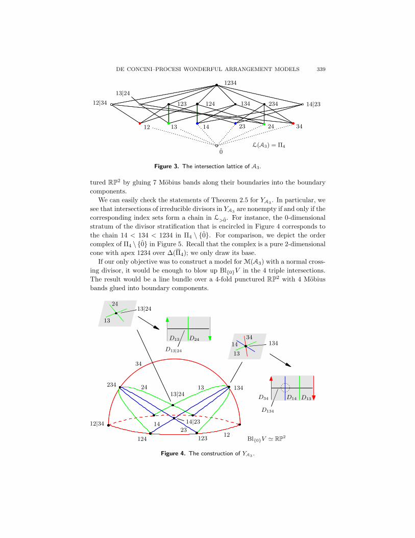
DE CONCINI–PROCESI WONDERFUL ARRANGEMENT MODELS 339
123
L(A3) = Π4
0
1413
13|24
234 14|23
34242312
12|34
1234
134124
Figure 3. The intersection lattice of A3.
tured RP2 by gluing 7 Mobius bands along their boundaries into the boundary
components.
We can easily check the statements of Theorem 2.5 for YA3. In particular, we
see that intersections of irreducible divisors in YA3are nonempty if and only if the
corresponding index sets form a chain in L>0. For instance, the 0-dimensional
stratum of the divisor stratification that is encircled in Figure 4 corresponds to
the chain 14 < 134 < 1234 in Π4 \ {0}. For comparison, we depict the order
complex of Π4 \ {0} in Figure 5. Recall that the complex is a pure 2-dimensional
cone with apex 1234 over ∆(Π4); we only draw its base.
If our only objective was to construct a model for M(A3) with a normal cross-
ing divisor, it would be enough to blow up Bl{0}V in the 4 triple intersections.
The result would be a line bundle over a 4-fold punctured RP2 with 4 Mobius
bands glued into boundary components.
13
24
14
13
34134
D34
D134
13|24
D13
D13|24
D24
D14 D13
12|34
234
34
124
24 13
14|23
2314
12123
13413|24
Bl{0}V ' RP2
Figure 4. The construction of YA3.
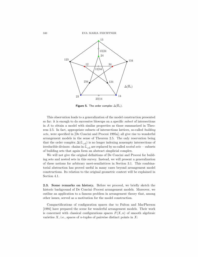
340 EVA MARIA FEICHTNER
12
123
13
24
134
34
234 124
23 14
∆(Π4)
12|34
13|24
23|14
Figure 5. The order complex ∆(Π4).
This observation leads to a generalization of the model construction presented
so far: it is enough to do successive blowups on a specific subset of intersections
in A to obtain a model with similar properties as those summarized in Theo-
rem 2.5. In fact, appropriate subsets of intersections lattices, so-called building
sets, were specified in [De Concini and Procesi 1995a]; all give rise to wonderful
arrangement models in the sense of Theorem 2.5. The only reservation being
that the order complex ∆(L>0) is no longer indexing nonempty intersections of
irreducible divisors: chains in L>0 are replaced by so-called nested sets — subsets
of building sets that again form an abstract simplicial complex.
We will not give the original definitions of De Concini and Procesi for build-
ing sets and nested sets in this survey. Instead, we will present a generalization
of these notions for arbitrary meet-semilattices in Section 3.1. This combina-
torial abstraction has proved useful in many cases beyond arrangement model
constructions. Its relation to the original geometric context will be explained in
Section 4.1.
2.3. Some remarks on history. Before we proceed, we briefly sketch the
historic background of De Concini–Procesi arrangement models. Moreover, we
outline an application to a famous problem in arrangement theory that, among
other issues, served as a motivation for the model construction.
Compactifications of configuration spaces due to Fulton and MacPherson
[1994] have prepared the scene for wonderful arrangement models. Their work
is concerned with classical configurations spaces F (X,n) of smooth algebraic
varieties X, i.e., spaces of n-tuples of pairwise distinct points in X:

DE CONCINI–PROCESI WONDERFUL ARRANGEMENT MODELS 341
F (X,n) = { (x1, . . . , xn) ∈ Xn |xi 6= xj for i 6= j}.
A compactification X[n] of F (X,n) is constructed in which the complement of
the original configuration space is a normal crossing divisor; in fact, X[n] has
properties analogous to those listed for arrangement models in Theorem 2.5. The
relation to the arrangement setting can be summarized by saying that, on the one
hand, the underlying spaces in the configuration space setting are incomparably
more complicated — smooth algebraic varieties X rather than real or complex
linear space; the combinatorics, on the other hand, is far simpler — it is the com-
binatorics of our basic Examples 2.4 and 2.6, the partition lattice Πn. The notion
of building sets and nested sets, which constitutes the defining combinatorics of
arrangement models, has its roots in the Fulton–MacPherson construction for
configuration spaces, hence is inspired by the combinatorics of Πn.
Looking along the time line in the other direction, De Concini–Procesi ar-
rangement models have triggered a number of more general constructions with
similar spirit: compactifications of conically stratified complex manifolds by
MacPherson and Procesi [1998], and model constructions for mixed real sub-
space and halfspace arrangements and real stratified manifolds by Gaiffi [2003]
that use spherical rather than classical blowups.
As a first impact, the De Concini–Procesi model construction has yielded
substantial progress on a longstanding open question in arrangement theory
[De Concini and Procesi 1995a, Section 5], the question being whether com-
binatorial data of a complex subspace arrangement determines the cohomology
algebra of its complement. For arrangements of hyperplanes, there is a beautiful
description of the integral cohomology algebra of the arrangement complement
in terms of the intersection lattice — the Orlik–Solomon algebra [1980]. Also,
a prominent application of Goresky and MacPherson’s Stratified Morse Theory
states that cohomology of complements of (complex and real) subspace arrange-
ments, as graded groups over Z, are determined by the intersection lattice and
its codimension labelling. In fact, there is an explicit description of cohomology
groups in terms of homology of intervals in the intersection lattice [Goresky and
MacPherson 1988, Part III]. However, whether multiplicative structure is deter-
mined as well remained an open question 20 years after it had been answered for
arrangements of hyperplanes (see [Feichtner and Ziegler 2000; Longueville 2000]
for results on particular classes of arrangements).
The De Concini–Procesi construction allows to apply Morgan’s theory on ra-
tional models for complements of normal crossing divisors [Morgan 1978] to ar-
rangement complements and to conclude that their rational cohomology algebras
indeed are determined by the combinatorics of the arrangement. A key step in
the description of the Morgan model is the presentation of cohomology of divisor
components and their intersections in purely combinatorial terms [De Concini
and Procesi 1995a, 5.1, 5.2]. For details on this approach to arrangement coho-
mology, see [De Concini and Procesi 1995a, 5.3].

342 EVA MARIA FEICHTNER
Unfortunately, the Morgan model is fairly complicated even for small arrange-
ments, and the approach is bound to rational coefficients. The model has been
considerably simplified in work of Yuzvinsky [2002; 1999]. In [Yuzvinsky 2002]
explicit presentations of cohomology algebras for certain classes of arrangements
were given. However, despite an explicit conjecture of an integral model for
arrangement cohomology in [Yuzvinsky 2002, Conjecture 6.7], extending the re-
sult to integral coefficients remained out of reach. Only years later, the ques-
tion has been fully settled to the positive in work of Deligne, Goresky and
MacPherson [Deligne et al. 2000] with a sheaf-theoretic approach, and paral-
lely by de Longueville and Schultz [2001] using rather elementary topological
methods: Integral cohomology algebras of complex arrangement complements
are indeed determined by combinatorial data.
3. The Combinatorial Core Data: A Step Beyond Geometry
We will now abandon geometry for a while and in this section fully concentrate
on combinatorial and algebraic gadgets that are inspired by De Concini–Procesi
arrangement models.
We first present a combinatorial analogue of De Concini–Procesi resolutions
on purely order theoretic level following [Feichtner and Kozlov 2004, Sections 2
and 3]. Based on the notion of building sets and nested sets for arbitrary lattices
proposed therein, we define a family of commutative graded algebras for any
given lattice.
The next Section then will be devoted to relate these objects to geometry—
to the original context of De Concini–Procesi arrangement models and, more
interestingly so, to different seemingly unrelated contexts in geometry.
3.1. Combinatorial resolutions. We will state purely combinatorial def-
initions of building sets and nested sets. Recall that, in the context of model
constructions, building sets list the strata that are to be blown up in the construc-
tion process, and nested sets describe beforehand the nonempty intersections of
irreducible divisor components in the final resolution.
Let L be a finite meet-semilattice, i.e., a finite poset such that any pair of ele-
ments has a unique maximal lower bound. In particular, such a meet-semilattice
has a unique minimal element that we denote with 0. We will talk about semilat-
tices for short. As a basic reference on partially ordered sets we refer to [Stanley
1997, Chapter 3].
Definition 3.1 (Combinatorial building sets). A subset G ⊆ L>0 in
a finite meet-semilattice L is called a building set if for any X ∈ L>0 and
max G≤X = {G1, . . . , Gk} there is an isomorphism of posets
ϕX :
k∏
j=1
[0, Gj ]∼=−→ [0, X] (3–1)

DE CONCINI–PROCESI WONDERFUL ARRANGEMENT MODELS 343
with ϕX(0, . . . , Gj , . . . , 0) = Gj for j = 1, . . . , k. We call FG(X) := max G≤X the
set of factors of X in G.
There are two extreme examples of building sets for any semilattice: we can
take the full semilattice L>0 as a building set. On the other hand, the set of
elements X in L>0 which do not allow for a product decomposition of the lower
interval [0, X] form the unique minimal building set (see Example 3.3 below).
Intuitively speaking, building sets are formed by elements in the semilattice
that are the perspective factors of product decompositions.
Any choice of a building set G in L gives rise to a family of so-called nested
sets. These are, roughly speaking, subsets of G whose antichains are sets of
factors with respect to the chosen building set. Nested sets form an abstract
simplicial complex on the vertex set G. This simplicial complex plays the role
of the order complex for arrangement models more general than the maximal
models discussed in Section 2.2.
Definition 3.2 (Nested sets). Let L be a finite meet-semilattice and G a
building set in L. A subset S in G is called nested (or G-nested if specification is
needed) if, for any set of incomparable elements X1, . . . , Xt in S of cardinality at
least two, the join X1 ∨ . . . ∨Xt exists and does not belong to G. The G-nested
sets form an abstract simplicial complex N(L,G), the nested set complex with
respect to L and G.
Observe that if we choose the full semilattice as a building set, then a subset is
nested if and only if it is linearly ordered in L. Hence, the nested set complex
N(L,L>0) coincides with the order complex ∆(L>0).
Example 3.3 (Building sets and nested sets for the partition lat-
tice). Choosing the maximal building set in the partition lattice Πn, we obtain
the order complex ∆((Πn) \ {0}) as the associated complex of nested sets. Topo-
logically, it is a cone over a wedge of (n− 1)! spheres of dimension n−1.
The minimal building set Gmin in Πn is given by partitions with at most one
block of size larger or equal 2, the so-called modular elements in Πn. We can
identify these partitions with subsets of {1, . . . , n} of size larger or equal 2. A
collection of such subsets is nested, if and only if none of the pairs of subsets
have a nontrivial intersection, i.e., for any pair of subsets they are either disjoint
or one is contained in the other. Referring to a naive picture of such containment
relation explains the choice of the term nested— it appeared first in the work
of Fulton and MacPherson [1994] on compactifications of classical configuration
spaces. As we noted earlier, the combinatorics they are concerned with is indeed
the combinatorics of the partition lattice.
For the rank 3 partition lattice Π3, maximal and minimal building sets co-
incide, G = Π3 \ {0}. The nested set complex N(Π3,G) is the order complex
∆(Π3 \ {0}) depicted in Figure 1.
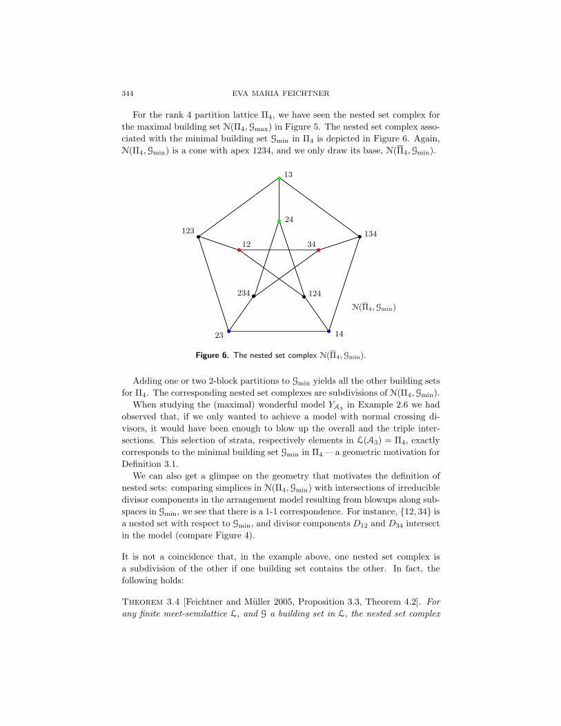
344 EVA MARIA FEICHTNER
For the rank 4 partition lattice Π4, we have seen the nested set complex for
the maximal building set N(Π4,Gmax) in Figure 5. The nested set complex asso-
ciated with the minimal building set Gmin in Π4 is depicted in Figure 6. Again,
N(Π4,Gmin) is a cone with apex 1234, and we only draw its base, N(Π4,Gmin).
N(Π4,Gmin)
1423
124234
34
134
24
13
123
12
Figure 6. The nested set complex N(Π4,Gmin).
Adding one or two 2-block partitions to Gmin yields all the other building sets
for Π4. The corresponding nested set complexes are subdivisions of N(Π4,Gmin).
When studying the (maximal) wonderful model YA3in Example 2.6 we had
observed that, if we only wanted to achieve a model with normal crossing di-
visors, it would have been enough to blow up the overall and the triple inter-
sections. This selection of strata, respectively elements in L(A3) = Π4, exactly
corresponds to the minimal building set Gmin in Π4 — a geometric motivation for
Definition 3.1.
We can also get a glimpse on the geometry that motivates the definition of
nested sets: comparing simplices in N(Π4,Gmin) with intersections of irreducible
divisor components in the arrangement model resulting from blowups along sub-
spaces in Gmin, we see that there is a 1-1 correspondence. For instance, {12, 34} is
a nested set with respect to Gmin, and divisor components D12 and D34 intersect
in the model (compare Figure 4).
It is not a coincidence that, in the example above, one nested set complex is
a subdivision of the other if one building set contains the other. In fact, the
following holds:
Theorem 3.4 [Feichtner and Muller 2005, Proposition 3.3, Theorem 4.2]. For
any finite meet-semilattice L, and G a building set in L, the nested set complex
DE CONCINI–PROCESI WONDERFUL ARRANGEMENT MODELS 345
N(L,G) is homotopy equivalent to the order complex of L>0,
N(L,G) ' ∆(L>0).
Moreover , if L is atomic, i .e., any element is a join of a set of atoms, and G and
H are building sets with G⊇H, then the nested set complex N(L,G) is obtained
from N(L,H) by a sequence of stellar subdivisions. In particular , the complexes
are homeomorphic.
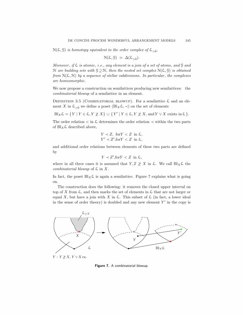
We now propose a construction on semilattices producing new semilattices: the
combinatorial blowup of a semilattice in an element.
Definition 3.5 (Combinatorial blowup). For a semilattice L and an ele-
ment X in L>0 we define a poset (BlXL,≺) on the set of elements
BlXL = {Y | Y ∈ L, Y 6≥ X} ∪ {Y ′ | Y ∈ L, Y 6≥ X, andY ∨X exists in L }.
The order relation < in L determines the order relation ≺ within the two parts
of BlXL described above,
Y ≺ Z, forY < Z in L,
Y ′ ≺ Z ′,forY < Z in L,
and additional order relations between elements of these two parts are defined
by
Y ≺ Z ′,forY < Z in L,
where in all three cases it is assumed that Y,Z 6≥ X in L. We call BlXL the
combinatorial blowup of L in X.
In fact, the poset BlXL is again a semilattice. Figure 7 explains what is going
on.
The construction does the following: it removes the closed upper interval on
top of X from L, and then marks the set of elements in L that are not larger or
equal X, but have a join with X in L. This subset of L (in fact, a lower ideal
in the sense of order theory) is doubled and any new element Y ′ in the copy is
BlXL
L≥X
Y : Y 6≥X, Y ∨X ex.
XY
Y ′
L
Figure 7. A combinatorial blowup.

346 EVA MARIA FEICHTNER
12′ 13′ 23′
Bl123Π3Π3
123
12 13 23 12 13 23
Figure 8. The combinatorial blowup of Π3 in 123.
defined to be covering the original element Y in L. The order relations in the
remaining, respectively the doubled, part of L stay the same as before.
In Figure 8 we give a concrete example: the combinatorial blowup of the
maximal element 123 in Π3, Bl123Π3. The result should be compared with
Figure 2. In fact, Bl123Π3 is the face poset of the divisor stratification in YA2=
Bl{0}V .
The following theorem shows that the three concepts introduced above— com-
binatorial building sets, nested sets, and combinatorial blowups— fit together so
as to provide a combinatorial analogue of the De Concini–Procesi model con-
struction.
Theorem 3.6 [Feichtner and Kozlov 2004, Theorem 3.4]. Let L be a semilattice,
G a combinatorial building set in L, and G1, . . . , Gt a linear order on G that is
nonincreasing with respect to the partial order on L. Then, consecutive combi-
natorial blowups in G1, . . . , Gt result in the face poset of the nested set complex
N(L,G):
BlGt(. . . (BlG2
(BlG1L)) . . .) = F(N(L,G)).
3.2. An algebra defined for atomic lattices. For any atomic lattice, we
define a family of graded commutative algebras based on the notions of building
sets and nested sets given above. Our exposition here and in Section 4.2 follows
[Feichtner and Yuzvinsky 2004]. Restricting our attention to atomic lattices is
not essential for the definition. However, for various algebraic considerations and
for geometric interpretations (compare Section 4.2) it is convenient to assume
that the lattice is atomic.
Definition 3.7. Let L be a finite atomic lattice, A(L) its set of atoms, and G
a building set in L. We define the algebra D(L,G) of L with respect to G as
D(L,G) := Z [{xG}G∈G]/
I,
where the ideal of relations I is generated by
t∏
i=1
xGifor {G1, . . . , Gt} 6∈ N(L,G) ,
∑
G≥H
xG for H ∈ A(L).

DE CONCINI–PROCESI WONDERFUL ARRANGEMENT MODELS 347
Observe that this algebra is a quotient of the face ring of the nested set com-
plex N(L,G).
Example 3.8 (Algebras associated to Π3 and Π4). For Π3 and its only
building set Gmax = Π3 \ {0}, the algebra reads as follows:
D(Π3,Gmax)=Z [x12, x13, x23, x123]/⟨
x12x13, x12x23, x13x23
x12 + x123, x13 + x123, x23 + x123
⟩
∼=Z [x123]/〈x2123〉.
For Π4 and its minimal building set Gmin, we obtain the following algebra after
simplifying slightly the presentation:
D(Π4,Gmin) ∼= Z [x123, x124, x134, x234, x1234]/
⟨ xijk x1234 for all 1 ≤ i < j < k ≤ 4
xijk xi′j′k′ for all ijk 6= i′j′k′
x2ijk + x2
1234 for all 1 ≤ i < j < k ≤ 4
⟩.
There is an explicit description for a Grobner basis of the ideal I, which in par-
ticular yields an explicit description for a monomial basis of the graded algebra
D(L,G).
Theorem 3.9. (1) [Feichtner and Yuzvinsky 2004, Theorem 2] The following
polynomials form a Grobner basis of the ideal I:∏
G∈S
xG for S 6∈ N(L,G),
k∏
i=1
xAi
( ∑
G≥B
xG
)d(A,B)
,
where A1, . . . , Ak are maximal elements in a nested set H ∈ N(L,G), B ∈ G
with B>A =∨k
i=1Ai, and d(A,B) is the minimal number of atoms needed
to generate B from A by taking joins.
(2) [Feichtner and Yuzvinsky 2004, Corollary 1] The resulting linear basis for
the graded algebra D(L,G) is given by the following set of monomials:∏
A∈S
xm(A)A ,
where S is running over all nested subsets of G, m(A) < d(A′, A), and A′ is
the join of S∩L<A.
Part (2) of Theorem 3.9 generalizes a basis description by Yuzvinsky [1997] for
D(L,G) in the case of G being the minimal building set in an intersection lattice
L of a complex hyperplane arrangement. Yuzvinsky’s basis description has also
been generalized in a somewhat different direction by Gaiffi [1997], namely for
closely related algebras associated with complex subspace arrangements.

348 EVA MARIA FEICHTNER
We will return to the algebra D(L,G) and discuss its geometric significance
in Section 4.2.
4. Returning to Geometry
4.1. Understanding stratifications in wonderful models. We first relate
the combinatorial setting of building sets and nested sets developed in Section 3.1
to its origin, the De Concini–Procesi model construction. Here is how to recover
the original notion of building sets [De Concini and Procesi 1995a, Definition in
§ 2.3], we call them geometric building sets, from our definitions:
Definition 4.1 (Geometric building sets). Let L be the intersection lattice
of an arrangement of subspaces in real or complex vector space V and cd : L → N
a function on L assigning the codimension of the corresponding subspace to each
lattice element. A subset G in L is a geometric building set if it is a building set
in the sense of 3.1, and for any X ∈ L the codimension of X is equal to the sum
of codimensions of its factors, FG(X):
cd (X) =∑
Y ∈FG(X)
cd (Y ).
An easy example shows that the notion of geometric building sets indeed is more
restrictive than the notion of combinatorial building sets. For arrangements of
hyperplanes, however, the notions coincide [Feichtner and Kozlov 2004, Propo-
sition 4.5.(2)].
Example 4.2 (Geometric versus combinatorial building sets). Let A
denote the following arrangement of 3 subspaces in R4:
A1 : x4 = 0, A2 : x1 = x2 = 0, A3 : x1 = x3 = 0.
The intersection lattice L(A) is a boolean algebra on 3 elements; we depict the
lattice with its codimension labelling in Figure 9. The set of atoms obviously is
a combinatorial building set. However, any geometric building set must contain
the intersection A2 ∩A3: its codimension is not the sum of codimensions of its
(combinatorial) factors A2 and A3.
L(A)
1 2 2
3 3
4
3
0
A1 A2 A3
A2 ∩A3
Figure 9. Geometric versus combinatorial building sets.

DE CONCINI–PROCESI WONDERFUL ARRANGEMENT MODELS 349
As we mentioned before, there are wonderful model constructions for arrange-
ment complements M(A) that start from an arbitrary geometric building set G
of the intersection lattice L(A) [De Concini and Procesi 1995a, 3.1]: In Def-
inition 2.2, replace the product on the right hand side of (2–1) by a product
over building set elements in L, and obtain the wonderful model YA,G by again
taking the closure of the image of M(A) under Ψ. In Definition 2.3, replace the
linear extension of Lop
>0by a nonincreasing linear order on the elements in G, and
obtain the wonderful model YA,G by successive blowups of subspaces in G, and
of proper transforms of such.
The key properties of these models are analogous to those listed in Theo-
rem 2.5, where in part (2), lattice elements are replaced by building set ele-
ments, and in part (3), chains in L as indexing sets of nonempty intersections of
irreducible components of divisors are replaced by nested sets. Hence, the face
poset of the stratification of YA,G given by irreducible components of divisors
and their intersections coincides with the face poset of the nested set complex
N(L,G). Compare Examples 2.6 and 3.3, where we found that nested sets with
respect to the minimal building set Gmin in Π4 index nonempty intersections of
irreducible divisor components in the arrangement model YA3,Gmin.
While the intersection lattice L(A) captures the combinatorics of the strat-
ification of V given by subspaces of A and their intersections, the nested set
complex N(L,G) captures the combinatorics of the divisor stratification of the
wonderful model YA,G. More than that: combinatorial blowups turn out to be
the right concept to describe the incidence change of strata during the construc-
tion of wonderful arrangement models by successive blowups:
Theorem 4.3 [Feichtner and Kozlov 2004, Proposition 4.7(1)]. Let A be a com-
plex subspace arrangement , G a geometric building set in L(A), and G1, . . . , Gt
a nonincreasing linear order on G. Let Bli(A) denote the result of blowing up
strata G1, . . . , Gi, for i ≤ t, and denote by Li the face poset of the stratification
of Bli(A) by proper transforms of subspaces in A and the exceptional divisors.
Then the poset Li coincides with the successive combinatorial blowups of L in
G1, . . . Gi:
Li = BlGi(. . . (BlG2
(BlG1L)) . . .).
Combinatorial building sets, nested sets and combinatorial blowups occur in
other situations and prove to be the right concept for describing stratifications
in more general model constructions. This applies to the wonderful conical com-
pactifications of MacPherson and Procesi [1998] as well as to models for mixed
subspace and halfspace arrangements and for stratified real manifolds by Gaiffi
[2003].
Also, combinatorial blowups describe the effect which stellar subdivisions in
polyhedral fans have on the face poset of the fans. In fact, combinatorial blowups
describe the incidence change of torus orbits for resolutions of toric varieties by

350 EVA MARIA FEICHTNER
consecutive blowups in closed torus orbits. This implies, in particular, that for
any toric variety and for any choice of a combinatorial building set in the face
poset of its defining fan, we obtain a resolution of the variety with torus orbit
structure prescribed by the nested set complex associated to the chosen building
set. We believe that such combinatorially prescribed resolutions can prove useful
in various concrete situations (see [Feichtner and Kozlov 2004, Section 4.2] for
further details).
There is one more issue about nested set stratifications of maximal wonder-
ful arrangement models that we want to discuss here, mostly in perspective of
applications in Section 5. According to Definition 2.2, any point in the model
YA can be written as a collection of a point in V and lines in V , one line for
each element in L(A). There is a lot of redundant information in this rendering,
e.g., points on the open stratum π−1(M(A)) are fully determined by their first
“coordinate entry”, the point in M(A) ⊆ V .
Here is a more economic encoding of a point ω on YA [Feichtner and Kozlov
2003, Section 4.1]: we find that ω can be uniquely written as
ω = (x,H1, `1,H2, `2, . . . ,Ht, `t) = (x, `1, `2, . . . , `t), (4–1)
where x is a point in V , the H1, . . . ,Ht form a descending chain of subspaces
in L>0, and the `i are lines in V . More specifically, x = π(ω), and H1 is the
maximal lattice element that, as a subspace of V , contains x. The line `1 is
orthogonal to H1 and corresponds to the coordinate entry of ω indexed by H1 in
P(V/H1). The lattice element H2, in turn, is the maximal lattice element that
contains both H1 and `1. The specification of lines `i, i.e., lines that correspond
to coordinates of ω in P(V/Hi), and the construction of lattice elements Hi+1,
continues analogously for i ≥ 2 until a last line `t is reached whose span with
Ht is not contained in any lattice element other than the full ambient space V .
Observe that the Hi are determined by x and the sequence of lines `i; we choose
to include the Hi in order to keep the notation more transparent.
The full coordinate information on ω can be recovered from (4–1) by setting
H0 =⋂
A, `0 = 〈x〉, and retrieving the coordinate ωH indexed by H ∈ L>0 as
ωH = 〈`j ,H〉/H ∈ P(V/H),
where j is chosen from {1, . . . , t} such that H ≤ Hj , but H 6≤ Hj+1.
A nice feature of this encoding is that for a given point ω in YA we can tell
the open stratum in the nested set stratification which contains it:
Proposition 4.4 [Feichtner and Kozlov 2003, Proposition 4.5]. A point ω in a
maximal arrangement model YA is contained in the open stratum indexed by the
chain H1>H2> . . . >Ht in L>0 if and only if its point/line description (4–1)
reads ω = (x,H1, `1,H2, `2, . . . ,Ht, `t).
DE CONCINI–PROCESI WONDERFUL ARRANGEMENT MODELS 351
4.2. A wealth of geometric meaning for D(L,G). We turn to the algebra
D(L,G) that we defined for any atomic lattice L and combinatorial building set
G in L in Section 3.2. We give two geometric interpretations for this algebra;
one is restricted to L being the intersection lattice of a complex hyperplane
arrangement and originally motivated the definition of D(L,G), the other applies
to any atomic lattice and provides for a somewhat unexpected connection to toric
varieties.
We comment briefly on the projective version of wonderful arrangement mod-
els that we need in this context (see [De Concini and Procesi 1995a, § 4] for
details). For any arrangement of linear subspaces A in V , a model for its pro-
jectivization PA = {PA | A ∈ A} in PV , i.e., for M(PA) = PV \⋃
PA, can
be obtained by replacing the ambient space V by its projectivization PV in the
model constructions 2.2 and 2.3. The constructions result in a smooth projective
variety that we denote by Y PA. A model Y P
A,G for a specific geometric building set
G in L can be obtained analogously. In fact, under the assumption that P(⋂
A)
is contained in the building set G, the affine model YA,G is the total space of a
(real or complex) line bundle over the projective model Y PA,G which is isomorphic
to the divisor component in YA,G indexed with⋂
A.
The most prominent example of a projective arrangement model is the min-
imal wonderful model for the complex braid arrangement, YACn−2
,Gmin. It is iso-
morphic to the Deligne–Knudson–Mumford compactification M0,n of the moduli
space of n-punctured complex projective lines [De Concini and Procesi 1995a,
4.3].
Here is the first geometric interpretation of D(L,G) in the case of L being the
intersection lattice of a complex hyperplane arrangement.
Theorem 4.5 [De Concini and Procesi 1995b; Feichtner and Yuzvinsky 2004].
Let L = L(A) be the intersection lattice of an essential arrangement of complex
hyperplanes A and G a building set in L which contains the total intersection
of A. Then, D(L,G) is isomorphic to the integral cohomology algebra of the
projective arrangement model Y PA,G:
D(L,G) ∼= H∗(Y PA,G,Z).
Example 4.6 (Cohomology of braid arrangement models). The pro-
jective arrangement model Y PA2
is homeomorphic to the exceptional divisor in
YA2= Bl{0}C
2, hence to CP1. Its cohomology is free of rank 1 in degrees 0 and
2 and zero otherwise. Compare with D(Π3,Gmax) in Example 3.8.
The projective arrangement model Y PA3,Gmin
is homeomorphic to M0,5, whose
cohomology is known to be free of rank 1 in degrees 0 and 4, free of rank 5 in
degree 2, and zero otherwise. At least the coincidence of ranks is easy to verify
in comparison with D(Π4,Gmin) in Example 3.8.
352 EVA MARIA FEICHTNER
Theorem 4.5 in fact gives an elegant presentation for the integral cohomology
of M0,n∼= Y P
An−2,Gminin terms of generators and relations:
H∗(M0,n) ∼= D(Πn−1,Gmin)
∼= Z [ {xS}S⊆[n−1],|S|≥2 ]/⟨ xS xT for S ∩ T 6= ?, S 6⊆T, T 6⊆S,
∑{i,j}⊆S
xS for 1≤ i< j≤n− 1
⟩.
A lot of effort has been spent on describing the cohomology of M0,n (see
[Keel 1992]), but none of the presentations comes close to the simplicity of the
one stated above.
A nice expression for the Hilbert function of H∗(M0,n) has been derived
in [Yuzvinsky 1997] as a consequence of a monomial linear basis for minimal
projective arrangement models presented there.
To propose a more general geometric interpretation for D(L,G), we start by de-
scribing a polyhedral fan Σ(L,G) for any atomic lattice L and any combinatorial
building set G in L.
Definition 4.7 (A simplicial fan realizing N(L,G)). Let L be an atomic
lattice with set of atoms A = {A1, . . . , An}, G a combinatorial building set in L.
For any G ∈ G define the characteristic vector vG in Rn by
(vG)i :=
{1 if G ≥ Ai,
0 otherwise,for i = 1, . . . , n.
The simplicial fan Σ(L,G) in Rn is the collection of cones
VS := cone{vG | G ∈ S}
for S nested in G.
By construction, Σ(L,G) is a rational, simplicial fan that realizes the nested set
complex N(L,G). The fan gives rise to a (noncompact) smooth toric variety
XΣ(L,G) [Feichtner and Yuzvinsky 2004, Proposition 2].
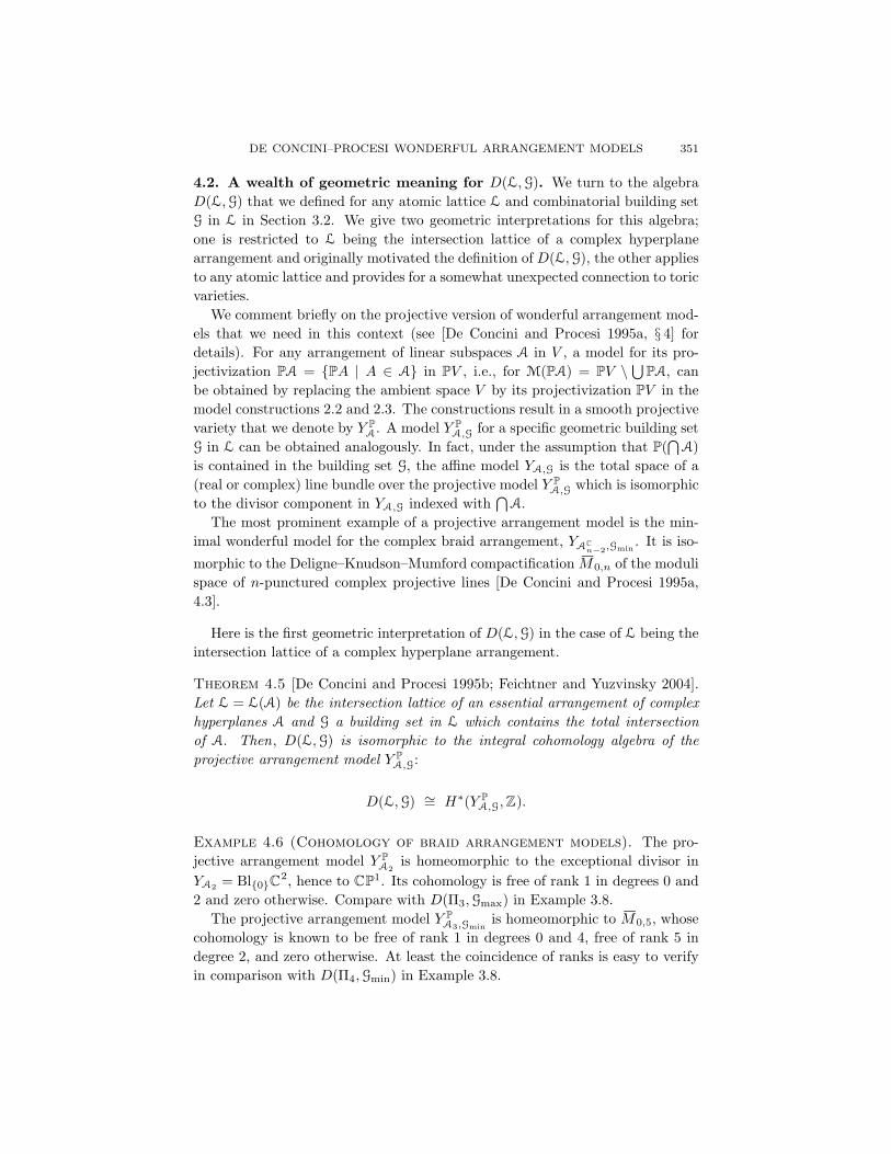
Example 4.8 (The fan Σ(Π3,Gmax) and its toric variety). We depict
Σ(Π3,Gmax) in Figure 10. The associated toric variety is the blowup of C3
in {0} with the proper transforms of coordinate axes removed.
v23
v123
v13
v12
Figure 10. The simplicial fan Σ(Π3,Gmax).

DE CONCINI–PROCESI WONDERFUL ARRANGEMENT MODELS 353
The algebra D(L,G) here gains another geometric meaning, this time for any
atomic lattice L. The abstract algebraic detour of considering D(L,G) in this
general setting is rewarded by a somewhat unexpected return to geometry:
Theorem 4.9 [Feichtner and Yuzvinsky 2004, Theorem 3]. For an atomic lattice
L and a combinatorial building set G in L, D(L,G) is isomorphic to the Chow
ring of the toric variety XΣ(L,G),
D(L,G) ∼= Ch∗(XΣ(L,G)).
5. Adding Arrangement Models to the Geometer’s Toolbox
Let a differentiable action of a finite group Γ on a smooth manifoldM be given.
The goal is to modify the manifold by blowups so as to have the group act on
the resolution M with abelian stabilizers— the quotient M/Γ then has much
more manageable singularities than the original quotient. Such modifications
for the sake of simplifying quotients have been of crucial importance at various
places. One instance is Batyrev’s work [1999] on stringy Euler numbers, which
in particular implies a conjecture of Reid [1992], and constitutes substantial
progress towards higher dimensional MacKay correspondence.
There are two observations that point to wonderful arrangement models as a
possible tool in this context. First, the model construction is equivariant if the
initial setting carries a group action: if a finite group Γ acts on a real or complex
vector space V , and the arrangement A is Γ-invariant, then the arrangement
model YA,G carries a natural Γ-action for any Γ-invariant building set G ⊆ L(A).
Second, the model construction is not bound to arrangements. In fact, locally
finite stratifications of manifolds which are local subspace arrangements, i.e.,
locally diffeomorphic to arrangements of linear subspaces, can be treated in a
fully analogous way. In the complex case, the construction has been pushed to
so-called conical stratifications in [MacPherson and Procesi 1998] with a real
analogue in [Gaiffi 2003].
The significance of De Concini–Procesi model constructions for abelianizing
group actions on complex varieties has been recognized by Borisov and Gunnells
[2002], following work of Batyrev [1999; 2000]. Here we focus on the real setting.
5.1. Learning from examples: permutation actions in low dimension.
Consider the action of the symmetric group Sn on real n-dimensional space by
permuting coordinates:
σ (x1, . . . , xn) = (xσ(1), . . . , xσ(n)) for σ ∈ Sn, x ∈ Rn.
Needless to say, we find a wealth of nonabelian stabilizers: For a point x ∈
Rn that induces the set partition π = (B1| . . . |Bt) of {1, . . . , n} by pairwise
coinciding coordinate entries, the stabilizer of x with respect to the permutation
action is the Young subgroup Sπ = SB1× . . .× SBt
of Sn, where SBidenotes
the symmetric subgroup of Sn permuting the coordinates in Bi for i = 1, . . . , t.
354 EVA MARIA FEICHTNER
The locus of nontrivial stabilizers for the permutation action of Sn, in fact, is
a familiar object: it is the rank (n−1) braid arrangement An−1. A natural idea
that occurs when trying to abelianize a group action by blowups is to resolve
the locus of nonabelian stabilizers in a systematic way. We look at some low-
dimensional examples.
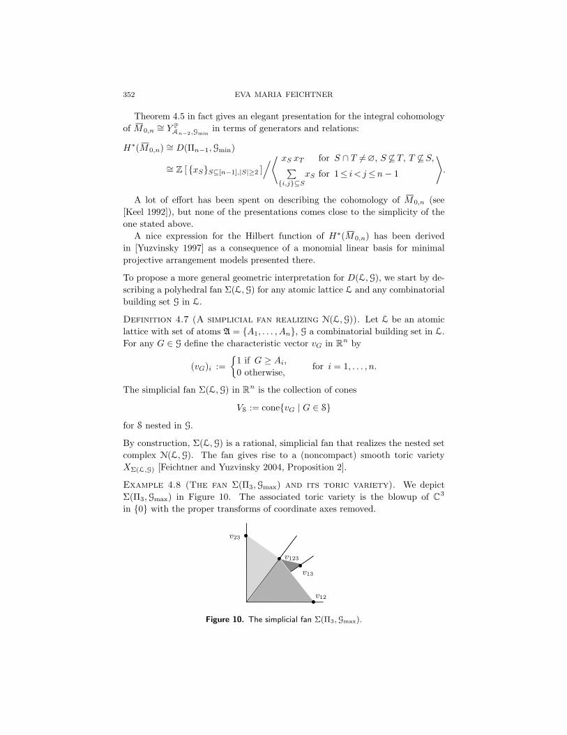
Example 5.1 (The permutation action of S3). We consider S3 acting
on real 2-space V ∼= R3/∆. The locus of nontrivial stabilizers consists of the 3
hyperplanes in A2: for x ∈ Hij \ {0}, stabx = 〈(ij)〉 ∼= Z2; in fact, 0 is the only
point having a nonabelian stabilizer, namely it is fixed by all of S3.
Blowing up {0} in V according to the general idea outlined above, we recognize
the maximal wonderful model for A2 that we discussed in Example 2.4.
H23
H12
H13
A2 ⊆ V YA2
stab (x, 〈x〉)=1
(x, 〈x〉)
ψ23 ψ13
x
(0, `)
ψ12
stab (y,H12)=〈(12)〉
y
stab (0, `)=1
stabψ12 = 〈(12)〉
(y,H12)
Figure 11. S3 acting on YA2.
By construction, S3 acts coordinate-wise on YA2. For points on proper trans-
forms of hyperplanes (y,Hij) ∈ Dij , 1 ≤ i < j ≤ 3, stabilizers are of or-
der two: stab (y,Hij) = 〈(ij)〉 ∼= Z2. Otherwise, stabilizers are trivial, unless
we are looking at one of the three points ψij marked in Figure 11. E.g., for
ψ12=(0, 〈(1,−1, 0)〉), stabψ12 = 〈(12)〉 ∼= Z2. Although the transposition (12)
does not fix the line 〈(1,−1, 0)〉) point-wise, it fixes ψ12 as a point in YA2! We
see that transpositions (ij) ∈ S3 act on the open Mobius band YA2by central
symmetries in ψij .
Observe that the nested set stratification is not fine enough to distinguish
stabilizers: as the points ψij show, stabilizers are not isomorphic on open strata.
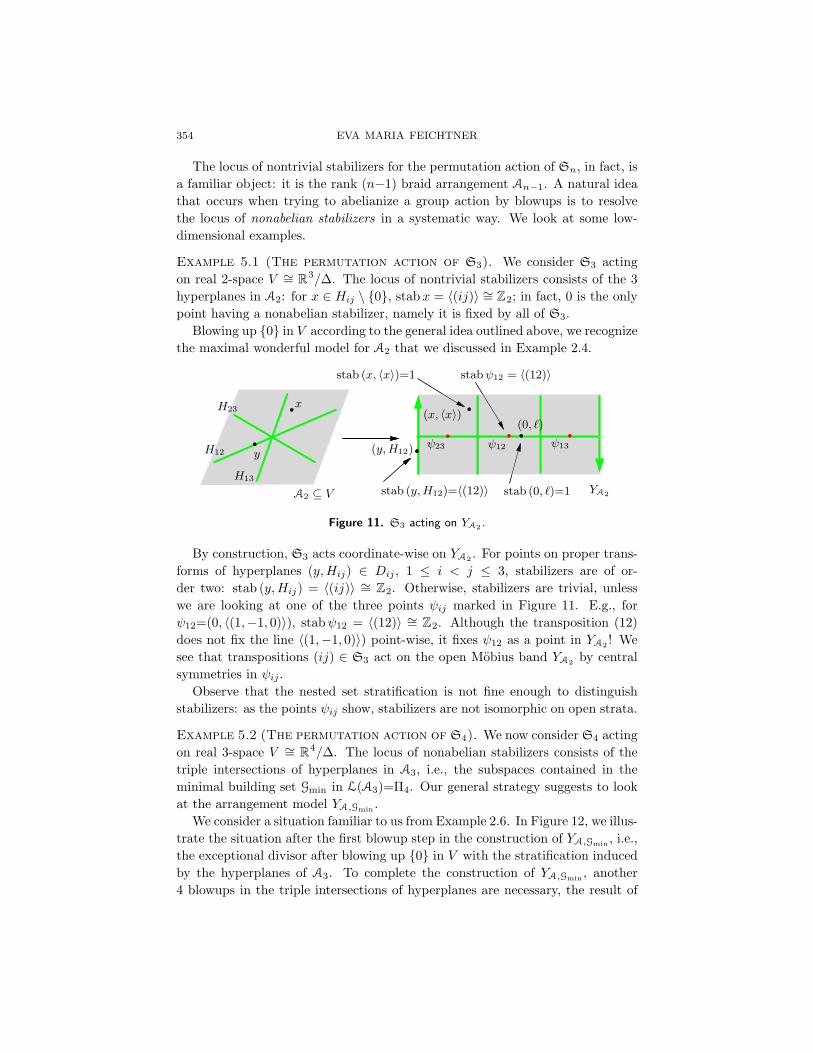
Example 5.2 (The permutation action of S4). We now consider S4 acting
on real 3-space V ∼= R4/∆. The locus of nonabelian stabilizers consists of the
triple intersections of hyperplanes in A3, i.e., the subspaces contained in the
minimal building set Gmin in L(A3)=Π4. Our general strategy suggests to look
at the arrangement model YA,Gmin.
We consider a situation familiar to us from Example 2.6. In Figure 12, we illus-
trate the situation after the first blowup step in the construction of YA,Gmin, i.e.,
the exceptional divisor after blowing up {0} in V with the stratification induced
by the hyperplanes of A3. To complete the construction of YA,Gmin, another
4 blowups in the triple intersections of hyperplanes are necessary, the result of

DE CONCINI–PROCESI WONDERFUL ARRANGEMENT MODELS 355
14
13
34134
D13
D34
D134
D14
12|34
234
34
124
13 134
14|23
2314
12312
ν=(0, 〈(1,−1,−1, 1)〉
(0, 〈(1,−1, 1,−1)〉)
2413|24
ω=(0, 〈(1,−1, 0, 0)〉
stab ν ∼= Z2 o Z2
stabω ∼= Z2 × Z2
Figure 12. S4 acting on Bl{0}V , where V = R4/∆.
which we illustrate locally for the triple intersection corresponding to 134. Triple
intersections of hyperplanes in Bl{0}V have stabilizers isomorphic to S3 — the
further blowups in triple intersections are indeed necessary to obtain an abelian-
ization of the permutation action.
Again, we observe that the nested set stratification on YA,Gmindoes not dis-
tinguish stabilizers: we indicate subdivisions of nested set strata resulting from
nonisomorphic stabilizers by dotted lines, respectively unfilled points in Fig-
ure 12.
We now look at stabilizers of points on the model YA,Gmin. We find points
with stabilizers isomorphic to Z2 — any generic point on a divisor Dij will be
such. We also find points with stabilizers isomorphic to Z2 × Z2, e.g., the point
ω on D1234 corresponding to the line 〈(1,−1, 0, 0)〉.
But, on YA,Gminwe also find points with nonabelian stabilizers! For example,
the intersection ofD14 andD23 onD1234 corresponding to the line 〈(1,−1,−1, 1)〉
is stabilized by both (14) and (12)(34) in S4, which do not commute. In fact,
the stabilizer is isomorphic to Z2 oZ2.
This observation shows that blowing up the locus of nonabelian stabilizers is
not enough to abelianize the action! Further blowups in double intersections of
hyperplanes are necessary, which suggests, contrary to our first assumption, the
maximal arrangement model YA3as an abelianization of the permutation action.
Some last remarks on this example: observe that stabilizers of points on YA3
all are elementary abelian 2-groups. We will later see that the strategy of resolv-
ing finite group actions on real vector spaces and even manifolds by constructing
356 EVA MARIA FEICHTNER
a suitable maximal De Concini–Procesi model does not only abelianize the ac-
tion, but yields stabilizers isomorphic to elementary abelian 2-groups.
Also, it seems we cannot do any better than that within the framework of
blowups, i.e., we neither can get rid of nontrivial stabilizers, nor can we reduce
the rank of nontrivial stabilizers any further. The divisors Dij are stabilized
by transpositions (ij) which supports our first claim. For the second claim,
consider the point ω = (0, `1) in YA3with `1 = 〈(1,−1, 0, 0)〉 (here we use the
encoding of points on arrangement models proposed in (4–1)). We have seen
above that stabω ∼= Z2 × Z2, in fact stabω = 〈(12)〉 × 〈(34)〉. Blowing up YA3
in ω means to again glue in an open Mobius band. Points on the new exceptional
divisor Dω∼= RP1 will be parameterized by tupels (0, `1, `2), where `2 is a line
orthogonal to `1 in V . A generic point on this stratum will be stabilized only
by the transposition (12), specific points however, e.g., (0, `1, 〈(0, 0, 1,−1)〉) will
still be stabilized by all of stabω ∼= Z2 × Z2.
5.2. Abelianizing a finite linear action. Following the basic idea of propos-
ing De Concini–Procesi arrangement models as abelianizations of finite group
actions and drawing from our experiences with the permutation action on low-
dimensional real space in Section 5.1 we here treat the case of finite linear actions.
Let a finite group Γ act linearly and effectively on real n-space Rn. Without
loss of generality, we can assume that the action is orthogonal [Vinberg 1989,
Section 2.3, Theorem 1]; we fix the appropriate scalar product throughout.
Our strategy is to construct an arrangement of subspaces A(Γ) in real n-space,
and to propose the maximal wonderful model YA(Γ) as an abelianization of the
given action.
Construction 5.3 (The arrangement A(Γ)). For any subgroup H in Γ,
define a linear subspace
L(H) := span{ ` | ` line in Rn with H ◦ ` = ` }, (5–1)
the linear span of all lines in V that are invariant under the action of H.
Denote by A(Γ) = A(Γ ˘ Rn) the arrangement of proper subspaces in R
n
that are of the form L(H) for some subgroup H in Γ.
Observe that the arrangement A(Γ) never contains any hyperplane: if L(H) were
a hyperplane for some subgroup H in Γ, then also its orthogonal line ` would be
invariant under the action of H. By definition of L(H), however, ` would then
be contained in L(H) which in turn would be the full ambient space.
Theorem 5.4 [Feichtner and Kozlov 2005, Thm. 3.1]. For any effective linear
action of a finite group Γ on n-dimensional real space, the maximal wonderful
arrangement model YA(Γ) abelianizes the action. Moreover , stabilizers of points
on the arrangement model are isomorphic to elementary abelian 2-groups.
The first example coming to mind is the permutation action of Sn on real n-
space. We find that A(Sn) is the rank 2 truncation of the braid arrangement,

DE CONCINI–PROCESI WONDERFUL ARRANGEMENT MODELS 357
Ark≥2n−1 , i.e., the arrangement consisting of subspaces in An−1 of codimension at
least 2. For details, see [Feichtner and Kozlov 2005, Section 4.1]. In earlier work
[Feichtner and Kozlov 2003], we had already proposed the maximal arrangement
model of the braid arrangement as an abelianization of the permutation action.
We proved that stabilizers on YAn−1are isomorphic to elementary abelian 2-
groups by providing explicit descriptions of stabilizers based on an algebraic-
combinatorial set-up for studying these groups.
5.3. Abelianizing finite differentiable actions on manifolds. We now
look at a generalization of the abelianization presented in Section 5.2. Assume
that Γ is a finite group that acts differentiably and effectively on a smooth real
manifold M . We first observe that such an action induces a linear action of
the stabilizer stabx on the tangent space TxM at any point x in M . Hence,
locally we are back to the setting that we discussed before: For any subgroup
H in stabx, we can define a linear subspace L(x,H) := L(H) of the tangent
space TxM as in (5–1), and we can combine the nontrivial subspaces to form an
arrangement Ax := A(stab ˘ TxM) in TxM .
Combined with the information that a model construction in the spirit of
De Concini–Procesi arrangement models exists also for local subspace arrange-
ments, we need to stratify the manifold so as to locally reproduce the arrange-
ment Ax in any tangent space TxM . Here is how to do that:
Construction 5.5 (The stratification L). For any x ∈ M , and any sub-
group H in stabx, define a normal (!) subgroup F (x,H) in H by
F (x,H) = {h ∈ H | h ◦ y = y for any y ∈ L(x,H)};
F (x,H) is the subgroup of elements in H that fix all of L(x,H) point-wise.
Define L(x,H) to be the connected component of the fixed point set of F (x,H)
in M that contains x. Now combine these submanifolds so as to form a locally
finite stratification
L = (L(x,H))x∈M, H≤stab x.
Observe that, as we tacitly did for stratifications induced by arrangements or by
irreducible components of divisors, we only specify strata of proper codimension.
The stratification L locally coincides with the tangent space stratifications
coming from our linear setting. Technically speaking: for any x ∈M , there exists
an open neighborhood U of x in M , and a stabx-equivariant diffeomorphism
Φx : U → TxM such that
Φx(L(x,H)) = L(x,H) (5–2)
for any subgroup H in stabx. In particular, (5–2) shows that the stratification
L of M is a local subspace arrangement.
Theorem 5.6 [Feichtner and Kozlov 2005, Theorem 3.4]. Let a finite group Γ act
differentiably and effectively on a smooth real manifold M . Then the wonderful

358 EVA MARIA FEICHTNER
model YL induced by the locally finite stratification L of M abelianizes the action.
Moreover , stabilizers of points on the model YL are isomorphic to elementary
abelian 2-groups.
Example 5.7 (Abelianizing the permutation action on RP2). We take
a small nonlinear example: the permutation action of S3 on the real projective
plane induced by S3 permuting coordinates in R3.
We picture RP2 by its upper hemisphere model in Figure 13, where we agree
to place the projectivization of ∆⊥ on the equator. The locus of nontrivial
stabilizers of the S3 permutation action consists of the projectivizations of hy-
perplanes Hij :xi = xj , for 1 ≤ i < j ≤ 3, and three additional points Ψij on
P∆⊥ indicated in Figure 13. The S3 action can be visualized by observing that
transpositions (ij) ∈ S3 act as reflections in the lines PHij , respectively.
∆ = [1 : 1 : 1]
Ψ23 = [0 : 1 : −1][1 : −2 : 1]
Ψ12=[1 : −1 : 0]
[−2 : 1 : 1] Ψ13 = [1 : 0 : −1]
[1 : 1 : −2]
PH13
PH23
PH12
Figure 13. S3 acting on RP2: the stabilizer stratification.
We find that the arrangements A` in the tangent spaces T`RP2 are empty,
unless ` = [1:1:1]. Hence, (5–2) allows us to conclude that the L-stratification of
RP2 consists of a single point, [1:1:1]. Observe that the S3-action on T[1:1:1]RP2
coincides with the permutation action of S3 on R3/∆.
The wonderful model YL hence is a Klein bottle, the result of blowing up RP2
in [1:1:1], i.e., glueing a Mobius band into the punctured projective plane.
Observe that the L-stratification is coarser than the codimension 2 truncation
of the stabilizer stratification: The isolated points Ψij on P∆⊥ have nontrivial
stabilizers, but do not occur as strata in the L-stratification.
Acknowledgments
I thank the organizers of the Combinatorial and Discrete Geometry workshop
held at MSRI in November 2003, for creating an event of utmost breadth, a true
kaleidoscope of topics unified by the ubiquity of geometry and combinatorics.

DE CONCINI–PROCESI WONDERFUL ARRANGEMENT MODELS 359
References
[Batyrev 1999] V. V. Batyrev, “Non-Archimedean integrals and stringy Euler numbersof log-terminal pairs”, J. Eur. Math. Soc. 1:1 (1999), 5–33.
[Batyrev 2000] V. V. Batyrev, “Canonical abelianization of finite group actions”,preprint, 2000. Available at math.AG/0009043.
[Borisov and Gunnells 2002] L. A. Borisov and P. E. Gunnells, “Wonderful blowupsassociated to group actions”, Selecta Math. (N.S.) 8:3 (2002), 373–379.
[De Concini and Procesi 1995a] C. De Concini and C. Procesi, “Wonderful models ofsubspace arrangements”, Selecta Math. (N.S.) 1:3 (1995), 459–494.
[De Concini and Procesi 1995b] C. De Concini and C. Procesi, “Hyperplane arrange-ments and holonomy equations”, Selecta Math. (N.S.) 1:3 (1995), 495–535.
[Deligne et al. 2000] P. Deligne, M. Goresky, and R. MacPherson, “L’algebre decohomologie du complement, dans un espace affine, d’une famille finie de sous-espaces affines”, Michigan Math. J. 48 (2000), 121–136.
[Feichtner and Kozlov 2003] E. M. Feichtner and D. N. Kozlov, “Abelianizing the realpermutation action via blowups”, Int. Math. Res. Not. no. 32 (2003), 1755–1784.
[Feichtner and Kozlov 2004] E. M. Feichtner and D. N. Kozlov, “Incidence combina-torics of resolutions”, Selecta Math. (N.S.) 10:1 (2004), 37–60.
[Feichtner and Kozlov 2005] E. M. Feichtner and D. N. Kozlov, “A desingularizationof real differentiable actions of finite groups”, Int. Math. Res. Not. no. 15 (2005).
[Feichtner and Muller 2005] E. M. Feichtner and I. Muller, “On the topology of nestedset complexes”, Proc. Amer. Math. Soc. 133 (2005), 999–1006.
[Feichtner and Yuzvinsky 2004] E. M. Feichtner and S. Yuzvinsky, “Chow rings of toricvarieties defined by atomic lattices”, Invent. Math. 155:3 (2004), 515–536.
[Feichtner and Ziegler 2000] E. M. Feichtner and G. M. Ziegler, “On cohomologyalgebras of complex subspace arrangements”, Trans. Amer. Math. Soc. 352:8 (2000),3523–3555.
[Fulton and MacPherson 1994] W. Fulton and R. MacPherson, “A compactification ofconfiguration spaces”, Ann. of Math. (2) 139:1 (1994), 183–225.
[Gaiffi 1997] G. Gaiffi, “Blowups and cohomology bases for De Concini-Procesi modelsof subspace arrangements”, Selecta Math. (N.S.) 3:3 (1997), 315–333.
[Gaiffi 2003] G. Gaiffi, “Models for real subspace arrangements and stratified mani-folds”, Int. Math. Res. Not. no. 12 (2003), 627–656.
[Goresky and MacPherson 1988] M. Goresky and R. MacPherson, Stratified Morse
theory, vol. 14, Ergebnisse der Mathematik und ihrer Grenzgebiete (3) [Results inMathematics and Related Areas (3)], Springer, Berlin, 1988.
[Keel 1992] S. Keel, “Intersection theory of moduli space of stable n-pointed curves ofgenus zero”, Trans. Amer. Math. Soc. 330:2 (1992), 545–574.
[Longueville 2000] M. de Longueville, “The ring structure on the cohomology ofcoordinate subspace arrangements”, Math. Z. 233:3 (2000), 553–577.
[Longueville and Schultz 2001] M. de Longueville and C. A. Schultz, “The cohomologyrings of complements of subspace arrangements”, Math. Ann. 319:4 (2001), 625–646.
360 EVA MARIA FEICHTNER
[MacPherson and Procesi 1998] R. MacPherson and C. Procesi, “Making conicalcompactifications wonderful”, Selecta Math. (N.S.) 4:1 (1998), 125–139.
[Morgan 1978] J. W. Morgan, “The algebraic topology of smooth algebraic varieties”,
Inst. Hautes Etudes Sci. Publ. Math. no. 48 (1978), 137–204.
[Orlik and Solomon 1980] P. Orlik and L. Solomon, “Combinatorics and topology ofcomplements of hyperplanes”, Invent. Math. 56:2 (1980), 167–189.
[Reid 1992] M. Reid, “The MacKay correspondence and the physicists’ Euler number”,lecture notes, University of Utah and MSRI, 1992.
[Stanley 1997] R. P. Stanley, Enumerative combinatorics, vol. 1, Cambridge Studies inAdvanced Mathematics 49, Cambridge University Press, Cambridge, 1997.
[Vinberg 1989] E. B. Vinberg, Linear representations of groups, Basler Lehrbucher 2,Birkhauser, Basel, 1989.
[Yuzvinsky 1997] S. Yuzvinsky, “Cohomology bases for the De Concini–Procesi modelsof hyperplane arrangements and sums over trees”, Invent. Math. 127:2 (1997), 319–335.
[Yuzvinsky 1999] S. Yuzvinsky, “Rational model of subspace complement on atomiccomplex”, Publ. Inst. Math. (Beograd) (N.S.) 66(80) (1999), 157–164.
[Yuzvinsky 2002] S. Yuzvinsky, “Small rational model of subspace complement”, Trans.
Amer. Math. Soc. 354:5 (2002), 1921–1945.
Eva Maria FeichtnerDepartment of MathematicsETH Zurich8092 ZurichSwitzerland