dcef: deep collaborative encoder framework for

arX

iv:1

906.

0517

3v1

[cs

.LG

] 1

2 Ju

n 20

191

DCEF: Deep Collaborative Encoder Framework for

Unsupervised ClusteringJielei Chu, member, IEEE, Hongjun Wang, Jing Liu, Zeng Yu, Tianrui Li, Senior member, IEEE,

Abstract—Collaborative representation is a popular featurelearning approach, which encoding process is assisted by varietytypes of information. In this paper, we propose a collaborativerepresentation restricted Boltzmann Machine (CRRBM) for mod-eling binary data and a collaborative representation Gaussianrestricted Boltzmann Machine (CRGRBM) for modeling real-valued data by applying a collaborative representation strategyin the encoding procedure. We utilize Locality Sensitive Hashing(LSH) to generate similar sample subsets of the instance andobserved feature set simultaneously from input data. Hence, wecan obtain some mini blocks, which come from the intersectionof instance and observed feature subsets. Then we integrateContrastive Divergence and Bregman Divergence methods withmini blocks to optimize our CRRBM and CRGRBM models.In their training process, the complex collaborative relationshipsbetween multiple instances and features are fused into the hiddenlayer encoding. Hence, these encodings have dual characteristicsof concealment and cooperation. Here, we develop two deepcollaborative encoder frameworks (DCEF) based on the CRRBMand CRGRBM models: one is a DCEF with Gaussian linearvisible units (GDCEF) for modeling real-valued data, and theother is a DCEF with binary visible units (BDCEF) for mod-eling binary data. We explore the collaborative representationcapability of the hidden features in every layer of the GDCEFand BDCEF framework, especially in the deepest hidden layer.The experimental results show that the GDCEF and BDCEFframeworks have more outstanding performances than the classicAutoencoder framework for unsupervised clustering task on theMSRA-MM2.0 and UCI datasets, respectively.

Index Terms—restricted Boltzmann machine; collaborativerepresentation; Contrastive Divergence; Bregman Divergence;deep collaborative learning; unsupervised clustering.

I. INTRODUCTION

Collaborative representation (CR) originates the influential

sparse representation-based classification (SRC) [1].

Approaches based on CR have achieved effective performance

on classification [2]–[7], target detection [8] and face

recognition [9]–[11]. They developed various collaborative

strategies in the process of collaborative representation. Some

studies focused on the source of superior performance of the

CR [12], [13].

Recently, some works [14], [15], [16], [17], [18], [19]

focus on deep collaborative learning (DCL). There are

various novel deep collaborative models which have been

successfully applied in practice. In [14], a novel DCL

method is applied in multimodal brain development study

Jielei Chu, Hongjun Wang, Tianrui Li and Zeng Yu are with the Schoolof Information Science and Technology, Southwest Jiaotong University,Chengdu, 611756, Sichuan, China. e-mails: {jieleichu, wanghongjun, zyu,trli}@swjtu.edu.cn.

Jing Liu is with the School of Business, Sichuan University, Sichuan,610065, Chengdu, China. e-mail: [email protected]

to address some limitations of conventional data-fusion

methods. The traditional methods can not obtain complex

nonlinear relationship between multiple data. So, Hu et al.

[14] proposed a neural network framework to extract complex

crossdata relationships. The DCL method first uses a deep

neural network to represent original data, then designs a

collaborative learning layer using collaborative regression

to seek their correlations and link the data representation

with phenotypical information. In this method, the deep

learning process and collaborative learning belong to two

separate processes. Zhang et al. [15] developed a novel deep

architecture termed Self-and-Collaborative Attention Network

(SCAN) based on the convolutional neural networks (CNN)

for video person re-identification. The SCAN contains two

kinds of subnetworks: a self attention subnetwork (SAN) to

enhance feature representation and a collaborative attention

subnetwork (CAN) to select frames from probe based on

the representation of the other one. In [16], Liu et al.

presented a collaborative deconvolutional neural network (C-

DCNN) to jointly model two problems of single-view depth

estimation and semantic segmentation in computer vision.

Two deconvolutional neural networks (DCNNs) compose a

C-DCNN and the depth features and semantic are combined

in a unified deep network. In the training process, the depth

features and semantic are integrated together to benefit each

other. For face photo-sketch synthesis, Zhu et al. [17] proposed

a deep collaborative framework. It has two opposite networks

that can utilize the mutual interaction of two opposite

mappings, which are constrained by a collaborative loss. Li

et al. [18] developed a Deep Collaborative Embedding (DCE)

model for social image understanding task. It incorporates

the collaborative factor analysis and end-to-end learning

in one unified framework for the optimal compatibility of

latent space discovery and representation learning. The DCE

model integrates the tag correlation, image correlation and

weakly-supervised image-tag correlation simultaneously and

seamlessly to collaboratively explore the rich information of

social images. Xie et al. [19] proposed multi-view knowledge-

based collaborative (MV-KBC) deep model for benign and

malignant lung nodule classification. The model learns the

characteristics of 3-D lung nodule by decomposing a 3-D

nodule into nine views. A knowledge-based collaborative

(KBC) submodel is constructed from each view. Then the nine

KBC submodels are jointly used to classify lung nodules.

Various novel models have been proposed for deep

collaborative filtering. Fu et al. [20] developed a novel

deep learning method to promote the effectiveness of

intelligent recommendation system by understanding the

http://arxiv.org/abs/1906.05173v1

2

items beforehand and users. The low-dimensional vectors of

items and users are learned separately in the initial stage.

Then, in the prediction stage, the interaction between item

and user is simulated by a feed-forward neural networks.

Chae et al. [21] proposed a novel Collaborative Adversarial

Autoencoders (CAAE) framework, which extends the

conventional GraphGAN and IRGAN. The Autoencoder as

one of the most successful DNNs is the generator and the

Bayesian personalized ranking (BPR) is the discriminative

model of CAAE framework. Zeng et al. [22] developed a

Deep Collaborative Filtering (DCF) model, which integrated

matrix completion and deep representation learning. Yue et

al. [23] proposed a novel denoising method via deep fusion

of convolutional and collaborative filtering for high ISO

JPEG images. The proposed method fuses the strengths of

collaborative and convolutional filtering using a deep CNN.

Our motivation is that how to develop some variants of

RBMs to make them have the capabilities of collaborative

representation. On this basis, we hope to develop some

deep collaborative encoding frameworks with these variants

of RBMs to explore the capabilities of deep collaborative

representation. It’s a known fact that classical RBM has

been proven to be an excellent feature representation model

[24], [25]. Then more and more researchers focus on

various variants of standard RBM [26]–[36]. And many

deep networks based on classical RBM and its variants are

developed [37]–[44]. They have achieved great success in

practical applications. However, previous studies have hardly

considered CR in the process of feature learning of RBM.

Then, the capability of feature representation of it is subject to

some limitations. Furthermore, the deep encoding framework

based on RBMs (e.g. Autoencoder) has not capability of

collaborative representation.

In this paper, two types of collaborative representation

RBMs are proposed to represent hidden and collaborative

features: one is a collaborative representation restricted

Boltzmann Machine (CRRBM) for modeling binary data and

the other is a collaborative representation Gaussian restricted

Boltzmann Machine (CRGRBM) for modeling real-valued

data. Locality Sensitive Hashing (LSH) [45] is employed to

generate similar sample subsets of the instance and observed

feature set simultaneously from input data. Hence, some

mini blocks are obtained, which come from the intersection

of instance and observed feature subsets. Then Contrastive

Divergence and Bregman Divergence methods are integrated

with mini blocks to optimize our CRRBM and CRGRBM

models. To extract deep hidden and collaborative features,

two types of deep collaborative encoder frameworks (DCEF)

based on the CRRBM and CRGRBM models are proposed:

one is a DCEF with Gaussian linear visible units (GDCEF)

for modeling real-valued data, and the other is a DCEF with

binary visible units (BDCEF) for modeling binary data. The

collaborative representation capability of the hidden features

in every layer of the GDCEF and BDCEF frameworks are

exploited, especially on the deepest hidden layer.

To best of our knowledge, our work is the first one to

explore collaborative representation capability of RBMs

by developing variants of classic RBMs and extract

deep collaborative hidden features by constructing deep

Collaborative Encoder Frameworks. Our major contributions

of this paper are summarized as follows:

• A collaborative representation restricted Boltzmann Ma-

chine (CRRBM) and a collaborative representation Gaus-

sian restricted Boltzmann Machine (CRGRBM) models

are developed to represent hidden and collaborative fea-

tures for binary and real-valued data, respectively.

• Contrastive Divergence and Bregman Divergence meth-

ods are integrated to optimize the proposed CRRBM

and CRGRBM models. The hidden collaborative features

of the proposed CRRBM and CRGRBM models fuse

complex relationship of multi-instances and observed

features (mini blocks) of the input data.

• Two novel deep Collaborative Encoder Frameworks (GD-

CEF and BDCEF) based on CRRBM and CRGRBM

models are proposed for exploiting deep collaborative

features for unsupervised clustering. On each hidden layer

of the proposed GDCEF and BDCEF, their more powerful

capabilities of extracting deep collaborative features are

exploited, especially on the deepest hidden layer.

The remaining of the paper is organized as follows. The theo-

retical background is described in Section II. Two collaborative

representation RBMs are developed in Section III. A learning

algorithm of CRRBM model is given in Section IV. Two deep

collaborative encoder frameworks are proposed in SectionV.

The experimental results are shown in Section VI. Finally,

our contributions are summarized in Section VII.

II. THEORETICAL BACKGROUND

A. Restricted Boltzmann Machine

1) Binary Visible Units: For classic RBMs [24], its archi-

tecture is a shallow two-layer structure, which consists of a

binary visible and hidden layer. The energy function of RBMs

is defined by:

E(v,h) = −∑

i∈visibles

aivi −∑

j∈hiddens

bjhj −∑

i,j

vihjwij ,

(1)

where v and h are the visible and hidden layer vectors,

respectively, vi and hj are the binary visible and hidden units,

respectively, wij is the symmetric connection weight between

them, ai and bj are the biases of visible and hidden units,

respectively.

Given a visible vector v, the binary state hj is equal to 1

with probability

p(hj = 1|v) = σ(bj +∑

i

viwij), (2)

where σ(x) = 11+exp(−x)) , which is a logistic sigmoid func-

tion.

Similarly, given a hidden vector h, an unbiased sample of

the binary state vi is equal to 1 with probability

p(vi = 1|h) = σ(ai +∑

j

hjwij). (3)

3

Because it is difficult to get an unbiased sample of <

vihj >model, Hinton proposed a faster learning algorithm

by Contrastive Divergence (CD) [25], [26] method. Then the

update rules of parameters is given by:

∆wij = ε(< vihj >data − < vihj >recon), (4)

∆ai = ε(< vi >data − < vi >recon), (5)

∆bj = ε(< hj >data − < hj >recon), (6)

where ε is learning rate.

2) Gaussian Linear Visible Units: For modeling real-valued

data, the binary visible units are replaced by Gaussian linear

visible units. This energy function becomes:

E(v,h) =−∑

i∈visibles

(vi − ai)2

2σ2i

−∑

j∈hiddens

bjhj

−∑

i,j

vi

σi

hjwij ,

(7)

where σi is the standard deviation of the Gaussian noise for

visible unit i. It is difficult to use CD method to learn the

variance of the noise. In practice, we normalise the original

data to have unit variance and zero mean. So, the reconstructed

result of a Gaussian linear visible unit is equal to the input

from hidden binary units plus the bias.

B. Encoder Framework of Autoencoder

1) Classic Autoencoder: The framework of Autoencoder

[37] consists of a stack of RBMs, which is shown in Fig. 1

(right one). In the encoding process of the Autoencoder, the

learned hidden features of one RBM are used as the input

for training the next one. This layer-by-layer learning is an

effective method to train the deep Autoencoder model. The

processes of encoder and decoder are nonlinear transformation

(sigmoid transformation).

2) Autoencoder with Gaussian Linear visible Units: To

model real-valued data, the binary units of visible layer of

Autoencoder can be replaced by Gaussian linear visible units,

which is shown in Fig. 1 (left one). The training method is

still a layer-by-layer learning pattern. The process of encoder

is still sigmoid transformation, but the top decoder is a linear

transformation.

III. THE MODEL OF COLLABORATIVE REPRESENTATION

RBM

The major goal of classic RBMs is to learn hidden layer

features from the original data, with the connection matrix W

serving as the mapping between the data and hidden features.

In their processes of training, only the relationship between

instances (rows) is usually considered. In many cases the

hidden features we wish to obtain is often rather collaborative

representation both of instances and features. In this work,

the original data matrix is divided into many small blocks by

means of Locality Sensitive Hashing (LSH) [45] method which

exploits similar samples by a weak hash function. In this way,

similar instances and features cluster together in relative big

row and column blocks, respectively. Then, one after another

Encoding

EncodingEncoding

Encoding

RBM

GRBM

RBM

W1

W2

W3

Autoencoder

RBM

RBM

RBM

W1

W2

W3

V

h1

V

h1

h2

h3h3

h2

Linear visible units Binary visible units

Fig. 1. Left: A deep Autoencoder with Gaussian linear visible units forreal-valued data, which consists of a RBM with Gaussian linear visible units(GRBM) on the top layer and a stack of classic RBM on the down layer. Thelearned binary hidden features of GRBM are used as the input for trainingthe next RBM, then the learned hidden features of this RBM are used asthe input for training the following RBM in the stack. Right: A classic deepAutoencoder, which consists of a RBM stack, and the learned hidden layerfeatures of one RBM are used as the input for training the next one.

LSH

Block

Block Block

Block

Block Block

Block

Block

Block

Block

Block

Block Block

Block

Block

Block

Instances

(Row)

Features (Column)

Fig. 2. Example of Block partition: the rows and columns of visible datamatrix are partitioned into K(e.g.K = 4) row clusters and L(e.g.L = 4)column clusters by LSH. The same row and column clusters gather togetherand the overlaps (rows and columns) compose each block. Every red pointrepresents the center of each block. We use dashed lines to denote therecombination matrix (virtual matrix) of the original data.

small crossed blocks with rows and columns will appear (see

Fig. 2). Our expectation is that each block data possibly gather

towards its own center in collaborative representation space.

So, this improved RBM is called Collaborative Representation

RBM (CRRBM). Supposing that the CRRBM has Gaussian

linear visible units, we call it Collaborative Representation

GRBM (CRGRBM). Next, the crucial problem we need to

solve is that how to model the variant RBMs and obtain the

update rules of the model parameters.

Let D = {v1,v2, · · · ,vN} be an original data set

with N vectors and M features of each vector. The vis-

ible layer vector vs = (vs1, vs2, · · · , vsi, · · · , vsM ), (i =1, 2, · · · ,M, s = 1, 2, · · · , N). The hidden layer vector

4

hs = (hs1, hs2, · · · , hsj , · · · , hsM ′), (j = 1, 2, · · · ,M ′, s =

1, 2, · · · , N). The reconstructed visible layer vector v(r)s =

(v(r)s1 , v

(r)s2 , · · · , v

(r)si , · · · , v

(r)sM ), (i = 1, 2, · · · ,M, s =

1, 2, · · · , N). The reconstructed hidden layer vector h(r)s =

(h(r)s1 , h

(r)s2 , · · · , h

(r)sj , · · · , h

(r)sM ), (j = 1, 2, · · · ,M ′, s =

1, 2, · · · , N). The matrix (vT1 v

T2 · · ·vT

N )T is partitioned into

K row clusters by LSH and each cluster has a serial number

set of vectors ℜk, (k = 1, 2, · · · ,K and ℜ1 ∪ ℜ2 · · · ∪ ℜK ={1, 2, · · · , N}). Simultaneously, the matrix is partitioned into

L column clusters by LSH and each cluster has a serial number

set of vectors ℓl, (l = 1, 2, · · · , L and ℓ1 ∪ ℓ2 · · · ∪ ℓK ={1, 2, · · · ,M}). So, the matrix is divided into K ×L blocks.

Based on the expectations of our collaborative representa-

tion method and the training objective of classic RBM, our

novel objective function takes the form:

G(V, θ) =

−η

N

∑

vi

logp(vi;θ) +(1− η)

K × L

[

K∑

k=1

L∑

l=1

∑

s∈ℜk

∑

t∈ℓl

d(hst, ukl)

+

K∑

k=1

L∑

l=1

∑

s∈ℜk

∑

t∈ℓl

d(h(r)st , u

(r)kl )

]

,

(8)

where θ = {a, b,W} are the model parameters, η is an

adjusting parameter, d(hst, ukl) and d(h(r)st , u

(r)kl ) are the Breg-

man divergences [46] [47] distances, which are defined as:

d(hst, ukl) = (hst − ukl)2 and d(h

(r)st , u

(r)kl ) = (h

(r)st − u

(r)kl )

2,

respectively. ukl and u(r)kl are the centers of block (ℜk, ℓl) in

hidden layer and reconstructed hidden layer, respectively. They

take the form:

ukl =

∑

s∈ℜk

∑

t∈ℓl

hst

|ℜk||ℓl|, u

(r)kl =

∑

s∈ℜk

∑

t∈ℓl

h(r)st

|ℜk||ℓl|.

(9)

IV. THE ALGORITHM

Here, we introduce the gradient descent algorithm and an

analysis of its complexity in detail.

A. Learning Algorithm

To optimize the above model by gradient descent algorithm,

some variables are fixed first. Then the remaining variables

are updated by an iterative method. The learning algorithm is

shown in Algorithm I.

Suppose that

Cdata =

K∑

k=1

L∑

l=1

∑

s∈ℜk

∑

t∈ℓl

(hst − ukl)2, (10)

Crecon =

K∑

k=1

L∑

l=1

∑

s∈ℜk

∑

t∈ℓl

(h(r)st − u

(r)kl )

2. (11)

Using the introduced variables Cdata and Crecon, the ob-

jective function have another concise equivalent form:

G(V, θ) =

−η

N

∑

vi

logp(vi;θ) +(1− η)

K × L(Cdata + Crecon).

(12)

The following crucial problem is that how to solve this

multi-objective optimization problem. For the average log-

likelihood ηN

∑

vi

logp(vi;θ), the CD method was presented to

approximately follow the gradient of two divergences CDn =KL(p0||p∞) − KL(pn||p∞) to avoid enormous difficulties of

the log-likelihood gradient computing. Normally, we run the

Markov chain from the data distribution p0 to p1 (one step) in

CD learning. So, the following key task is how to obtain the

approximative gradient of Cdata + Crecon.

Suppose that Jdata = hst − ukl, Jrecon = h(r)st − u

(r)kl , then

Jdata = hst −

∑

s∈ℜk

∑

t∈ℓl

hst

|ℜk||ℓl|= σ

(

M∑

m=1

vsmwmt + bst)

−

∑

s∈ℜk

∑

t∈ℓl

σ(

M∑

m=1vsmwmt + bst

)

|ℜk||ℓl|

(13)

and

Jrecon = h(r)st −

∑

s∈ℜk

∑

t∈ℓl

h(r)st

|ℜk||ℓl|= σ

(

M∑

m=1

v(r)smwmt + b(r)st

)

−

∑

s∈ℜk

∑

t∈ℓl

σ(

M∑

m=1v(r)smwmt + b

(r)st

)

|ℜk||ℓl|,

(14)

where σ is a sigmoid function.

When t = j ∈ ℓl, the partial derivative of Jdata is given by:

∂Jdata

∂wij

=e−

( M∑

m=1vsmwmj+bsj

)

vsi[

1 + e−(

M∑

m=1vsmwmj+bsj)

]2

−

∑

s∈ℜk

e−

(

M∑

m=1vsmwmj+bsj

)

vsi[

1+e−(

M∑

m=1vsmwmj+bsj)

]2

|ℜk|

=(1− hsj)hsjvsi −

∑

s∈ℜk

(1− hsj)hsjvsi

|ℜk|

(15)

Obviously, if t 6= j, then ∂Jdata

∂wij= 0.

Similarly, if t = j ∈ ℓl, the partial derivative of Jrecon is

given by:

∂Jrecon

∂wij

= (1 − h(r)sj )h

(r)sj v

(r)si −

∑

s∈ℜk

(1− h(r)sj )h

(r)sj v

(r)si

|ℜk|(16)

As for model parameter b, if t = j, the partial derivative takes

the forms:

∂Jdata

∂bj= (1 − hsj)hsj −

∑

s∈ℜk

(1 − hsj)hsj

|ℜk|,

∂Jrecon

∂bj= (1− h

(r)sj )h

(r)sj −

∑

s∈ℜk

(1− h(r)sj )h

(r)sj

|ℜk|.

(17)

5

It is obvious that model parameter a is independent of Jdataand Jrecon. So, we can obtain that ∂Jdata

∂ai= 0 and ∂Jrecon

∂ai=

0. Then, the partial derivative of the Cdata in terms of wij

takes the form:

∂Cdata

∂wij

=2

K∑

k=1

∑

s∈ℜk

(

hsj −

∑

s∈ℜk

hsj

|ℜk|

)

[

(1− hsj)hsjvsi

−

∑

s∈ℜk

(1− hsj)hsjvsi

|ℜk|

]

.

(18)

And the partial derivative of the Crecon in terms of wij takes

the form:

∂Crecon

∂wij

=2

K∑

k=1

∑

s∈ℜk

(

h(r)sj −

∑

s∈ℜk

h(r)sj

|ℜk|

)

[

(1 − h(r)sj )h

(r)sj v

(r)si

−

∑

s∈ℜk

(1− h(r)sj )h

(r)sj v

(r)si

|ℜk|

]

.

(19)

Similarly, the partial derivative of the Cdata in terms of bj is

given by:

∂Cdata

∂bj=2

K∑

k=1

∑

s∈ℜk

(

hsj −

∑

s∈ℜk

hsj

|ℜk|

)

[

(1− hsj)hsj

−

∑

s∈ℜk

(1− hsj)hsj

|ℜk|

]

.

(20)

And the partial derivative of the Crecon in terms of bj is given

by:

∂Crecon

∂bj=2

K∑

k=1

∑

s∈ℜk

(

h(r)sj −

∑

s∈ℜk

h(r)sj

|ℜk|

)

[

(1 − h(r)sj )h

(r)sj

−

∑

s∈ℜk

(1− h(r)sj )h

(r)sj

|ℜk|

]

.

(21)

Combined with the CD learning with 1 step Gibbs sampling,

the update rule of the proposed model parameter W takes the

forms:

w(τ+1)ij = w

(τ)ij + ηε(< vihj >data − < vihj >recon)

+2(1− η)

K × L

{

K∑

k=1

∑

s∈ℜk

(

hsj −

∑

s∈ℜk

hsj

|ℜk|

)

[

(1− hsj)hsjvsi

−

∑

s∈ℜk

(1− hsj)hsjvsi

|ℜk|

]

+

K∑

k=1

∑

s∈ℜk

(

h(r)sj −

∑

s∈ℜk

h(r)sj

|ℜk|

)

[

(1 − h(r)sj )h

(r)sj v

(r)si −

∑

s∈ℜk

(1− h(r)sj )h

(r)sj v

(r)si

|ℜk|

]}

,

(22)

where ε is learning rate, the average < vihj >data and

< vihj >recon are computed using the sample data and

reconstructed data, respectively.

For the parameters of the biases a and b, the update rules

of them take the forms:

a(τ+1)i = a

(τ)i + ηε(< vi >data − < vi >recon), (23)

and

b(τ+1)j = b

(τ)j + ηε(< hj >data − < hj >recon)

+2(1− η)

K × L

{

K∑

k=1

∑

s∈ℜk

(

hsj −

∑

s∈ℜk

hsj

|ℜk|

)

[

(1− hsj)hsj

−

∑

s∈ℜk

(1 − hsj)hsj

|ℜk|

]

+

K∑

k=1

∑

s∈ℜk

(

h(r)sj −

∑

s∈ℜk

h(r)sj

|ℜk|

)

[

(1− h(r)sj )h

(r)sj −

∑

s∈ℜk

(1 − h(r)sj )h

(r)sj

|ℜk|

]}

.

(24)

Algorithm 1 Learning algorithm of CRRBM with 1 step

Gibbs sampling

Input:

D: input data sets;

B: training batch sets;

ε: learning rate;

(ℜk, ℓl): matrix blocks of D, k ∈ [1,K] and l ∈ [1, L];

Output:

θ: model parameters of CRRBM.

Initialize: a, b and W.

while τ not exceeding maximum iteration do

for all training batch B do

Encoder: sample the states of hidden units by Eq. (2).

Decoder: sample the reconstructed states of visible

units using Eq. (3).

for all ℜk do

for all ℓl do

Compute ∂Cdata

∂wijusing Eq. (18).

Compute ∂Crecon

∂wijusing Eq. (19).

Compute ∂Cdata

∂bjusing Eq. (20).

Compute ∂Crecon

∂bjusing Eq. (21).

end for

end for

Update parameter W using Eq. (22).

Update parameter a using Eq. (23).

Update parameter b using Eq. (24).

end for

τ = τ + 1.

end while

return a, b and W.

In the reconstruction process of CRGRBM model, a linear

reconstruction method replaces the nolinear reconstruction

method of CRRBM model. The steps of the learning algo-

rithms of our CRRBM and CRGRBM models are almost

6

the same, except the reconstruction process. So, we omit the

learning algorithm of CRGRBM model.

B. Complexity Analysis

In this subsection, we analyze the time complexity of above

learning algorithm. Supposing that the input data sets D is

divided into TB training batch. Then the time complexi-

ties of the encoder and decoder steps are O(TB) in each

iteration. When partial derivatives ∂Cdata

∂wij, ∂Crecon

∂wij, ∂Cdata

∂bj

and ∂Crecon

∂bjare calculated, they take O(TB × (K × L)) in

each iteration. The complexities of update parameters W ,

a and b are O(TB) in each iteration. Supposing that the

maximum iteration is IT . Then, the time complexity of the

CRRBM learning algorithm with 1 Step Gibbs sampling is

O(IT × TB × (K × L)).

V. DEEP COLLABORATIVE ENCODER FRAMEWORK

The classic RBMs and GRBMs have capabilities of hidden

layer feature representation for binary and real-valued data,

respectively. Moreover, our CRRBM and CRGRBM have

powerful capabilities of collaborative representation of hidden

features. To explore the superior collaborative representation

capability of deep networks for different data, two types of

deep encoder framework with three layers (see Fig. 3) are

constructed with the proposed CRRBM and CRGRBM as

building blocks of the deep framework.

For real-valued data, we construct a deep architecture

termed as Deep Collaborative Encoder Framework with Gaus-

sian linear visible units (GDCEF), which consists of one CR-

GRBM with Gaussian linear visible units and two CRRBMs

with binary visible units, as shown in Fig. 3. The learned

binary features of the CRGRBM are used as the input for

training the first CRRBM. Then the binary hidden features of

the first CRRBM are used as the input for training the next

CRRBM. The blocks for training the CRGRBM come from

the original real-valued data by LSH method. However, the

blocks for training the CRRBM come from the binary hidden

features by LSH method.

For binary data, we construct a deep architecture termed as

Deep Collaborative Encoder Framework with binary visible

units (BDCEF), which consists of three CRRBMs with binary

visible units, as shown in Fig. 3. The learned binary features

of the CRRBM are used as the input for training the next

CRRBM. The blocks for training the first CRRBM come from

the original data by LSH method. The blocks for training the

other CRRBMs come from the binary hidden features of the

upper CRRBM by LSH method.

VI. EXPERIMENT

To validate the collaborative representation performance

of the proposed GDCEF framework for real-valued data,

we conducted experiments on twelve image datasets of

the Microsoft Research Asia Multimedia (MSRA-MM) 2.0

[48] by unsupervised clustering. The properties of these

datasets are shown in Table I. For binary data, the proposed

Encoding

Encoding

Encoding

Encoding

CRRBM

CRGRBM

CRRBM

W1

W2

W3

Deep Collaborative Encoder Framework (DCEF)

CRRBM

CRRBM

CRRBM

W1

W2

W3

V

h1

V

h1

h2

h3h3

h2

GDCEF BDCEF

Fig. 3. Deep Collaborative Encoder Framework (DCEF). Left: A DCEF withGaussian linear visible units (GDCEF) for real-valued data, which consistsof a collaborative representation RBM with Gaussian linear visible units(CRGRBM) on the top layer and a stack of collaborative representation RBMwith binary visible units (CRRBM) on the down layer. The learned binaryhidden features of CRGRBM are used as the input for training the nextCRRBM, then the learned hidden features of CRRBM are used as the inputfor training the following CRRBM in the stack. Right: A DCEF with binaryvisible units (BDCEF) for binary data, which consists of a CRRBM stack,and the learned hidden layer features of one CRRBM are used as the inputfor training the next one.

BDCEF framework is used to assess the collaborative

representation performance by unsupervised clustering on

twelve UCI datasets. The details of them are shown in Table II.

A. Experimental Setting

In the following experiments, the deep Autoencoder [37]

is used to compare with our GDCEF and BDCEF networks.

For real-valued data, the Gaussian linear units are used in

visible layer of the deep Autoencoder. For the sake of fairness

in comparison, we use the same parameters of learning rate

in the GDCEF and the Autoencoder. For binary data, we

use classic deep Autoencoder with binary visible and hidden

units to compare the capabilities of feature representation

with our BDCEF framework. Similarly, we use the same

parameters of learning rate in the BDCEF and the classic

Autoencoder. In all experiments, the dimensionality of the data

and features remain the same. The experiments are divided

into three stages that are hidden layer features learning by

Autoencoder, GDCEF and BDCEF frameworks, unsupervised

clustering with the learned features and evaluations.

We use three popular external evaluations, e.g., accuracy

[49], Jaccard index [50] and Fowlkes and Mallows Index

(FMI) [51], to evaluate the performance of the proposed

GDCEF and BDCEF frameworks by unsupervised clustering

tasks. The accuracy [49] is an external evaluation metric,

which takes the form:

accuracy =

∑

i=1

δ(si,map(ri))

n,

(25)

where map(ri) maps label ri of each cluster to the equivalent

label and n is the total number of instances. If x = y , then

7

Data Autoencoder Feature

K-means

SC

Data GDCEFCollaborative

Feature

K-means

SC

Autoencoder-Kmean , Autoencoder-

SC algorithms framework

GDCEF-Kmean , GDCEF-SC

algorithms framework

Data BDCEFCollaborative

Feature

K-means

SC

BDCEF-Kmean , BDCEF-SC

algorithms framework

Fig. 4. The frameworks of contrast unsupervised clustering algorithms basedon Autoencoder (Autoencoder-Kmeans and Autoencoder-SC algorithms), GD-CEF (GDCEF-Kmeans and GDCEF-SC algorithms) and BDCEF (BDCEF-Kmeans and BDCEF-SC algorithms) framework.

δ(x, y) equals to 1 . Otherwise, it is zero. The Jaccard index

[50] metric is defined by:

Jac =|A ∩B|

|A ∪B|, (26)

where A and B are finite sample sets and 0 ≤ J(A,B) ≤ 1.

The FMI [51] as an external evaluation metric is given by:

FMI =

√

TP

TP + FP×

TP

TP + FN, (27)

where TP is the number of true positives, FP is the number

of false positives and and FN is the number of false negatives.

In the stage of unsupervised clustering , we use separately

K-means [52] and Spectral Clustering (SC) [53] algorithms

to evaluate the capabilities of feature representation of Au-

toencoder, GDCEF and BDCEF frameworks. The hidden

features of the Autoencoder are used as the input of K-means

and SC, so we call these contrastive clustering algorithms

Autoencoder-Kmeans and Autoencoder-SC, respectively. The

algorithm frameworks of them are shown in Fig. 4. Similarly,

The hidden features of the GDCEF and BDCEF are used as the

input of K-means and SC, we call these clustering algorithms

GDCEF-Kmeans, GDCEF-SC, BDCEF-Kmeans, BDCEF-SC,

respectively. The algorithm frameworks of them are shown in

Fig. 4.

B. GDCEF vs Autoencoder with Gaussian Linear Visible

Units by Unsupervised Clustering

In this section, we compare the collaborative representation

utility of the GDCEF framework with the Autoencoder on

the MSRA-MM2.0 [48] datasets by unsupervised clustering

and the experiments are duplicated ten times. In the GDCEF

TABLE ISUMMARY OF THE EXPERIMENT DATASETS I.

No. Dataset classes Instances features

1 banner 3 860 8922 beret 3 876 8923 bugat 3 882 8924 bugatti 3 882 8925 building 3 911 8926 vista 3 799 8997 vistawallpaper 3 799 8998 voituretuning 3 879 8999 water 3 922 89910 weddingring 3 897 89911 wing 3 856 89912 worldmap 3 935 899

TABLE IISUMMARY OF THE EXPERIMENT DATASETS II.

No. Dataset classes Instances features

1 balance 3 625 42 biodegradation 2 1055 413 car 4 1728 64 Climate Model 2 540 185 cred (Credit Approval) 2 690 156 dermatology 6 366 347 Haberman Survival 2 306 38 ILPD(Indian Liver Patient) 2 583 89 Kdd (1999 partial data) 3 1280 4110 OLD (Ozone Level Detection) 2 2534 7211 parkinsons 2 195 2212 secom 2 1567 590

framework, the visible units are Gaussian linear visible units,

so we use the same Gaussian linear units in the visible layer

of the Autoencoder.

Fig. 5 shows the comparison of clustering accuracies among

the original data, the deepest layer hidden features of the

Autoencoder and GDCEF framework on twelve image data

sets using K-means and SC algorithms. For every data set

on Table I, whether by K-means or SC clustering algorithms,

the hidden features of GDCEF shows better performance

than the hidden features of Autoencoder. In particular, the

data sets of banner, beret, building, vista and voituretuning

show outstanding performance on our GDCEF framework

for the K-means algorithm. For the SC algorithm, the data

sets of banner, bugat, bugatti, building, voituretuning, wing

and worldmap show excellent performance on the proposed

GDCEF framework. From the results of contrast experiments,

we are assured that our GDCEF framework has more powerful

capability of collaborative representation than the Autoencoder

with Gaussian linear visible units which has not any collabo-

rative representation strategy.

Fig. 6 shows the comparison of average clustering accura-

cies of all data sets in Table I in every layer (visible layer

data, the first layer hidden features, the second layer hidden

features and the third layer hidden features) of Autoencoder

and GDCEF by K-means and SC algorithms. For K-means

algorithm, the average accuracies are 0.4419, 0.4029, 0.4110

and 0.4087 from the visible to the deepest layer of the Autoen-

8

coder, respectively. There is little change of performance in

all hidden layers, furthermore, they show worse performance

than the visible layer. However, the average accuracies are

greatly raised to 0.5728, 0.5754 and 0.5987 from the first

to the deepest hidden layer of our GDCEF framework by

means of collaborative encoding strategy, respectively. For

SC algorithm, the average accuracies are 0.4058, 0.4820,

0.3794 and 0.3542 from the visible to the deepest layer

of the Autoencoder, respectively. It’s obvious that the first

hidden layer shows better performance than the visible layer.

Unfortunately, the performance of the Autoencoder gradually

declines as the layer increases. As shown in Fig. 6, the average

accuracies from the first to the deepest hidden layer are

0.4386, 0.4663 and 0.6330, respectively. Although the average

accuracy of the first hidden layer of GDCEF is worse than the

Autoencoder, the performance increases significantly as hidden

layer increases and the accuracy is eventually increased by

22.72%.

The detailed results of the clustering accuracies and vari-

ances on the GDCEF framework (the deepest hidden layer)

as shown in Table III. The inputs of the K-means and SC

algorithms are the original data. The Autoencoder-Kmeans

and Autoencoder-SC algorithms use the deepest hidden layer

(the third hidden layer) features of the Autoencoder as the

inputs. Similarly, the GDCEF-Kmeans and GDCEF-SC algo-

rithms use the deepest hidden layer (the third hidden layer)

features of the GDCEF framework as the inputs. The average

accuracies of GDCEF-Kmeans and GDCEF-SC algorithms are

0.5987 and 0.6330, respectively, which are 19% and 27.88%

higher than Autoencoder-Kmeans and the Autoencoder-SC

algorithms. Furthermore, they are 15.68% and 22.72% higher

than K-means and SC algorithms. The GDCEF-Kmeans algo-

rithm shows the best performance on the data sets of the ban-

ner, beret, building, vista, voituretuning and wing. Moreover,

GDCEF-SC algorithm shows the best performance on the data

sets of the bugat, bugatti, vistawallpaper, water, weddingring

and worldmap. As a whole, our GDCEF framework has

excellent capability of collaborative representation.

To prove the collaborative representation ability of our

GDCEF framework in more ways, Tables IV and V show the

results of the other two evaluating metrics of the Jaccard index

and FMI. On the whole, the average Jaccard index of K-means,

SC, Autoencoder-Kmeans and Autoencoder-SC algorithms are

0.4040, 0.2683, 0.2793 and 0.2563, respectively. But, the

GDCEF-Kmeans and GDCEF-SC algorithms raise the average

Jaccard index to 0.4424 and 0.5032, respectively. In Table

V, the average FMI of K-means, SC, Autoencoder-Kmeans

and Autoencoder-SC algorithms are 0.5715, 0.4354, 0.4444

and 0.4206, respectively. However, the GDCEF-Kmeans and

GDCEF-SC algorithms raise the average FMI to 0.6168 and

0.6864, respectively. Almost all data sets in Table I show the

best performance on the GDCEF framework by the evaluations

of Jaccard index and FMI except the data set of bugat.

From all above results of the experiments, our GDCEF

shows outstanding capability of collaborative representation.

C. BDCEF vs Autoencoder with Binary Visible Units by

Unsupervised Clustering

Here, we evaluate the collaborative representation perfor-

mance on the twelve UCI datasets by unsupervised clustering

in terms of the accuracy, Jaccard index and FMI evaluation

metrics. We compare our BDCEF framework with the Au-

toencoder, which has binary visible units.

Results for the comparison of clustering accuracies among

the original data, the deepest hidden layer features of the

Autoencoder and BDCEF framework by K-means and SC

algorithms are shown on Fig. 7. More detailed compar-

isons of K-means, SC, Autoencoder-Kmeans, Autoencoder-

SC, BDCEF-Kmeans and BDCEF-SC algorithms are shown in

Table VI. As a whole, the average accuracies of Autoencoder-

Kmeans and Autoencoder-SC algorithms without collabora-

tive strategy are 0.5951 and 0.6234, respectively. But, the

average accuracies of BDCEF-Kmeans and BDCEF-SC algo-

rithms based on our BDCEF framework are raised to 0.7122

and 0.7014, respectively. So, the collaborative representation

strategy improves the performance of BDCEF-Kmeans and

BDCEF-SC algorithms by 11.71% and 7.8%. For each data set

in Table II, the BDCEF-Kmeans algorithm shows outstanding

performance than other comparison algorithms on the data

sets of balance, biodegradation, cred, dermatology, ILDP,

Kdd, OLD, parkinsons and secom. The accuracies of them

are 0.6224, 0.6673, 0.6841, 0.4754, 0.8136, 0.9877, 0.9369,

0.8051 and 0.9336, respectively. Another algorithm based on

our BDCEF framework is BDCEF-SC, which shows excellent

performance than other comparison algorithms on the data sets

of car, ClimateModel and HabermanSurvival. The accuracies

of them are 0.6985, 0.9111 and 0.7255, respectively.

To explore the effect of collaborative representation strategy

in every hidden layer of our BDCEF framework, the com-

parison of average clustering accuracies of all data sets in

Table II are shown on the Fig. 8. The average accuracies

of the first hidden layer, the second hidden layer and the

third hidden layer are 0.6476, 0.6691 and 0.7122 by K-means

algorithm, respectively. As the hidden layers of our BDCEF

framework increase, the performances of them are increased

by 7.35%, 9.5% and 13.81%, respectively. For SC algorithm,

the average accuracies of the first, second and third hidden

layer are 0.6837, 0.6940 and 0.7014, respectively. Similarly,

as the hidden layer of our BDCEF framework increases, the

performances of them are increased by 14.02%, 15.05% and

15.79%, respectively. But, without the help of a collabora-

tive representation strategy, the average accuracies of the K-

means algorithm in the first, second and third layer of the

Autoencoder drop to 0.5864, 0.5986 and 0.5951, respectively,

in contrast with our BDCEF framework. Similarly, the average

accuracies of the SC algorithm in the first, second and third

layer of the Autoencoder drop to 0.6584, 0.6229 and 0.6234,

respectively.

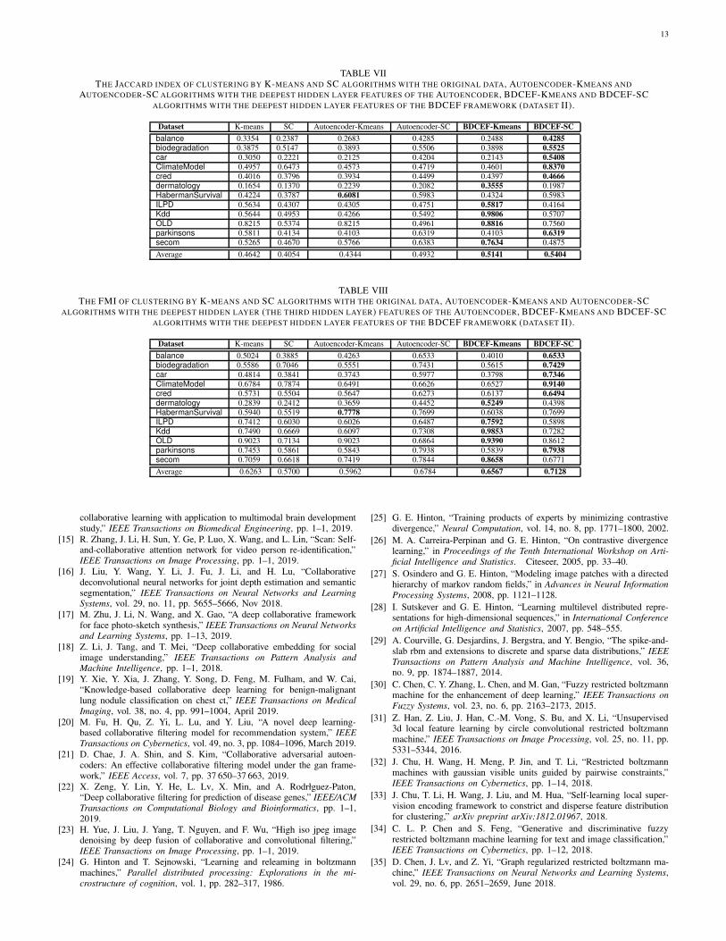
Table VII shows the results of Jaccard index on UCI data

sets. For BDCEF-Kmeans algorithm based on our BDCEF

framework, the data sets of dermatology, ILPD, Kdd, OLD

and secom show the best performance. The Jaccard indices

of them are 0.3555, 0.5817, 0.9806, 0.8816 and 0.7634,

9

Original data Autoencoder features GDCEF features0

0.2

0.4

0.6

0.8

1

1.2

0.4407

0.3616

0.5105

0.3570

0.9372 0.9349

Acc

urac

yDataset: banner

Clustering by K−meansClustering by SC


0.1

0.2

0.3

0.4

0.5

0.6

0.7

0.8

0.9

0.40750.3847 0.3893

0.3642

0.6895

0.4224

Acc

urac

y

Dataset: beret



0.1

0.2

0.3

0.4

0.5

0.6

0.7

0.8

0.39460.3730 0.3889

0.3515

0.4297

0.5748

Acc

urac

y

Dataset: bugat



0.1

0.2

0.3

0.4

0.5

0.6

0.7

0.8

0.9

0.42520.3832

0.4161

0.3639

0.4989

0.7007

Acc

urac

y

Dataset: bugatti



0.1

0.2

0.3

0.4

0.5

0.6

0.7

0.8

0.9

0.5719

0.49840.4501

0.3469

0.7146 0.7058

Acc

urac

y

Dataset: building



0.1

0.2

0.3

0.4

0.5

0.6

0.7

0.8

0.9

0.46930.4481

0.38420.3567

0.6308

0.5720

Acc

urac

y

Dataset: vista



0.1

0.2

0.3

0.4

0.5

0.6

0.7

0.8

0.43800.4593

0.3780 0.3717

0.4906

0.6320

Acc

urac

y

Dataset: vistawallpaper



0.1

0.2

0.3

0.4

0.5

0.6

0.7

0.8

0.4471

0.35040.3788

0.3481

0.6394 0.6359

Acc

urac

y

Dataset: voituretuning



0.1

0.2

0.3

0.4

0.5

0.6

0.7

0.8

0.40670.4252

0.3482 0.3449

0.5108

0.5705

Acc

urac

y

Dataset: water



0.1

0.2

0.3

0.4

0.5

0.6

0.7

0.3590

0.4002 0.4091

0.3456

0.4192

0.5217

Acc

urac

y

Dataset: weddingring



0.1

0.2

0.3

0.4

0.5

0.6

0.7

0.8

0.4731

0.40300.3680 0.3540

0.6192 0.6121

Acc

urac

y

Dataset: wing



0.1

0.2

0.3

0.4

0.5

0.6

0.7

0.8

0.9

0.4695

0.3829

0.4834

0.3455

0.6043

0.7134

Acc

urac

y

Dataset: worldmap


Fig. 5. The comparison of clustering accuracies among the original data, the deepest hidden features of Autoencoder and GDCEF by K-means and SCclustering algorithms. In this Autoencoder deep networks, the visible layer units are Gaussian linear units.

respectively. For BDCEF-SC algorithm based on the proposed

BDCEF framework, the data sets of balance, biodegradation,

car, ClimateModel, cred and parkinsons show the best per-

formance. The Jaccard indices of them are 0.4285, 0.5525,

0.5408, 0.8370, 0.4666 and 0.6319, respectively. Only one

data set (HabermanSurvival) shows the best performance in

Autoencoder-Kmeans algorithm.

Table VIII shows the results of FMI on UCI data sets. For

BDCEF-Kmeans algorithm, there are five data sets (dermatol-

ogy, ILPD, Kdd, OLD and secom) show the best performance.

The FMI of them are 0.5249, 0.7592, 0.9853, 0.9390 and

0.8658, respectively. For BDCEF-SC algorithm, there are six

other data sets (balance, biodegradation, car, ClimateModel,

cred and parkinsons) show best performance. Only one data

set (HabermanSurvival) shows outstanding performance in

Autoencoder-Kmeans algorithm.

From above the results of comparison experiments, all three

selected evaluation metrics show better performance on our

BDCEF framework than classic Autoencoder framework in

the capability of the features representation.

10

Visible Layer Hidden layer−1 Hidden layer−2 Hidden layer−30

0.1

0.2

0.3

0.4

0.5

0.6

0.7

0.8

0.4419 0.44190.4029

0.5728

0.4110

0.5754

0.4087

0.5987

Ave

rage

acc

urac

y

Clustering by K−means on dataset I

AutoencoderGDCEF


0.1

0.2

0.3

0.4

0.5

0.6

0.7

0.8

0.4058 0.4058

0.48200.4386

0.3794

0.4663

0.3542

0.6330

Ave

rage

acc

urac

y

Clustering by SC on dataset I

AutoencoderGDCEF

Fig. 6. The comparison of average clustering accuracies of all data sets in Table I among the original data, the first hidden layer features, the second hiddenlayer features and the third hidden layer features of Autoencoder and GDCEF by K-means and SC clustering algorithms. In this Autoencoder deep networks,the visible layer units are Gaussian linear units.

TABLE IIITHE ACCURACIES AND VARIANCES OF CLUSTERING BY K-MEANS AND SC ALGORITHMS WITH THE ORIGINAL DATA, AUTOENCODER-KMEANS AND

AUTOENCODER-SC ALGORITHMS WITH THE DEEPEST HIDDEN LAYER FEATURES OF THE AUTOENCODER, GDCEF-KMEANS AND GDCEF-SCALGORITHMS WITH THE DEEPEST HIDDEN LAYER FEATURES OF THE GDCEF FRAMEWORK (DATASET I).

Dataset K-means SC Autoencoder-Kmeans Autoencoder-SC GDCEF-Kmeans GDCEF-SC

banner 0.4407±0.0006 0.3616±0.0000 0.5105± 0.0004 0.3570±0.0000 0.9372±0.0046 0.9349±0.0089

beret 0.4075±0.0011 0.3847±0.0001 0.3893± 0.0018 0.3642±0.0001 0.6895±0.0132 0.4224±0.0112

bugat 0.3946±0.0003 0.3730±0.0001 0.3889± 0.0038 0.3515±0.0000 0.4297±0.0004 0.5748±0.0117

bugatti 0.4252±0.0007 0.3832±0.0000 0.4161± 0.0010 0.3639±0.0002 0.4989±0.0028 0.7007±0.0089

building 0.5719±0.0021 0.4984±0.0009 0.4501± 0.0013 0.3469±0.0001 0.7146±0.0000 0.7058±0.0026

vista 0.4693±0.0001 0.4481±0.0003 0.3842± 0.0006 0.3567±0.0001 0.6308±0.0015 0.5720±0.0068

vistawallpaper 0.4380±0.0001 0.4593±0.0001 0.3780± 0.0008 0.3717±0.0002 0.4906±0.0008 0.6320±0.0054

voituretuning 0.4471±0.0005 0.3504±0.0000 0.3788± 0.0013 0.3481±0.0001 0.6394±0.0139 0.6359±0.0025

water 0.4067±0.0001 0.4252±0.0000 0.3482± 0.0009 0.3449±0.0001 0.5108±0.0014 0.5705±0.0044

weddingring 0.3590±0.0004 0.4002±0.0004 0.4091±0.0010 0.3456±0.0001 0.4192±0.0061 0.5217±0.0024

wing 0.4731±0.0016 0.4030±0.0004 0.3680±0.0010 0.3540±0.0001 0.6192±0.0053 0.6121±0.0046

worldmap 0.4695±0.0021 0.3829±0.0000 0.4834± 0.0020 0.3455±0.0001 0.6043±0.0030 0.7134±0.0081

Average 0.4419 0.4058 0.4087 0.3542 0.5987 0.6330

TABLE IVTHE JACCARD INDEX OF CLUSTERING BY K-MEANS AND SC ALGORITHMS WITH THE ORIGINAL DATA, AUTOENCODER-KMEANS AND

AUTOENCODER-SC ALGORITHMS WITH THE DEEPEST HIDDEN LAYER FEATURES OF THE AUTOENCODER, GDCEF-KMEANS AND GDCEF-SCALGORITHMS WITH THE DEEPEST HIDDEN LAYER FEATURES OF THE GDCEF FRAMEWORK (DATASET I).


banner 0.6898 0.3197 0.3720 0.3192 0.8820 0.8779

beret 0.3573 0.2622 0.2825 0.2633 0.5348 0.5328

bugat 0.5081 0.2660 0.2668 0.2600 0.2801 0.4000

bugatti 0.5081 0.2653 0.2774 0.2606 0.3194 0.5420

building 0.3489 0.2961 0.3070 0.2629 0.5574 0.5470

vista 0.3301 0.2757 0.2582 0.2435 0.4738 0.4120

vistawallpaper 0.3301 0.2808 0.2796 0.2432 0.2714 0.4736

voituretuning 0.3022 0.2444 0.2515 0.2435 0.4760 0.4709

water 0.3081 0.2411 0.2321 0.2321 0.3561 0.4351

weddingring 0.2551 0.2421 0.2615 0.2393 0.2574 0.3274

wing 0.3986 0.2519 0.2491 0.2430 0.4714 0.4598

worldmap 0.5110 0.2744 0.3145 0.2647 0.4290 0.5602

Average 0.4040 0.2683 0.2793 0.2563 0.4424 0.5032

VII. CONCLUSIONS

In this work, two novel variants of collaborative represen-

tation RBM (CRRBM and CRGRBM) were presented for

modeling binary and real-valued input data, respectively. On

these bases, two novel deep collaborative encoding framework

(GDCEF and BDCEF) were proposed that target (1) real-

valued data and (2) binary data. We used the GDCEF and

BDCEF framework to show how our collaborative strategy

can yield superior performance in the feature representation

process. The Autoencoder with Gaussian linear visible units

was used to compare our GDCEF for unsupervised clus-

tering on the MSRA-MM2.0 datasets. Another Autoencoder

with binary visible units was used to compare our BDCEF

for unsupervised clustering on UCI datasets. In the contrast

experiments, we compared not only the deepest layer of

Autoencoder, GDCEF and BDCEF, but also the performance

of every layer (visible layer, the first hidden layer, the second

hidden layer and the third hidden layer). The GDCEF and

BDCEF frameworks showed fairly competitive results without

any fine-tuning of the model parameters for clustering tasks

on the twelve image data sets and UCI data sets, respectively.

In the future work, we will study how many hidden layers

11

Original data Autoencoder features BDCEF features0

0.1

0.2

0.3

0.4

0.5

0.6

0.7

0.8

0.5232

0.3888 0.3904

0.4640

0.6224

0.4640

Acc

urac

yDataset: balance



0.1

0.2

0.3

0.4

0.5

0.6

0.7

0.8

0.9

0.58860.6246 0.6199

0.6645 0.6673 0.6645

Acc

urac

y

Dataset: biodegradation



0.1

0.2

0.3

0.4

0.5

0.6

0.7

0.8

0.9

1

0.34720.3137

0.3414

0.5434

0.4426

0.6985

Acc

urac

y

Dataset: car



0.2

0.4

0.6

0.8

1

1.2

0.5111

0.7833

0.5130

0.59260.5500

0.9111

Acc

urac

y

Dataset: Climate Model Simulation Crashes



0.1

0.2

0.3

0.4

0.5

0.6

0.7

0.8

0.9

1

0.5623 0.5826

0.6652

0.6087

0.68410.6391

Acc

urac

y

Dataset: cred



0.1

0.2

0.3

0.4

0.5

0.6

0.29230.3115

0.4372

0.3552

0.47540.4508

Acc

urac

y

Dataset: dermatology



0.1

0.2

0.3

0.4

0.5

0.6

0.7

0.8

0.9

1

0.5000 0.5196

0.6242

0.7255

0.6275

0.7255

Acc

urac

y

Dataset: Haberman Survival



0.2

0.4

0.6

0.8

1

0.6947

0.5386

0.6844

0.5111

0.8136

0.6690

Acc

urac

y

Dataset: ILPD



0.2

0.4

0.6

0.8

1

1.2

0.66720.7039

0.5523

0.6414

0.9877

0.8156

Acc

urac

y

Dataset: Kdd



0.2

0.4

0.6

0.8

1

1.2

0.9017

0.6701

0.9065

0.7932

0.93690.9013

Acc

urac

y

Dataset: OLD



0.1

0.2

0.3

0.4

0.5

0.6

0.7

0.8

0.9

1

0.54360.5795

0.6359

0.76410.8051

0.7641

Acc

urac

y

Dataset: parkinsons



0.2

0.4

0.6

0.8

1

1.2

0.7569

0.5061

0.77090.8175

0.9336

0.7128

Acc

urac

y

Dataset: secom


Fig. 7. The comparison of clustering accuracies among the original data, the deepest hidden features of Autoencoder and BDCEF by K-means and SCclustering algorithms. In this Autoencoder deep networks, the visible layer units are binary units.

and dimensions would result in further improvements in per-

formance of the deep collaborative encoding framework.

VIII. ACKNOWLEDGEMENT

This work were partially supported by the National

Science Foundation of China (Nos. 61773324, 61573292,

61876158) and Sichuan Science and Technology Program

(2019YFS0432).

REFERENCES

[1] J. Wright, A. Y. Yang, A. Ganesh, S. S. Sastry, and Y. Ma, “Robust facerecognition via sparse representation,” IEEE Transactions on Pattern

Analysis and Machine Intelligence, vol. 31, no. 2, pp. 210–227, Feb2009.

[2] C. Zheng and N. Wang, “Collaborative representation with k-nearestclasses for classification,” Pattern Recognition Letters, vol. 117, pp. 30– 36, 2019.

[3] W. Li, Q. Du, and M. Xiong, “Kernel collaborative representation withtikhonov regularization for hyperspectral image classification,” IEEE

Geoscience and Remote Sensing Letters, vol. 12, no. 1, pp. 48–52, Jan2015.

[4] X. Chen, S. Li, and J. Peng, “Hyperspectral imagery classification withmultiple regularized collaborative representations,” IEEE Geoscience

and Remote Sensing Letters, vol. 14, no. 7, pp. 1121–1125, July 2017.

[5] J. Yang and J. Qian, “Hyperspectral image classification via multiscalejoint collaborative representation with locally adaptive dictionary,” IEEE

12


0.1

0.2

0.3

0.4

0.5

0.6

0.7

0.8

0.9

0.5741 0.5741 0.5864

0.64760.5986

0.6691

0.5951

0.7122

Ave

rage

acc

urac

y

Clustering by K−means on dataset II

AutoencoderBDCEF


0.1

0.2

0.3

0.4

0.5

0.6

0.7

0.8

0.9

0.5435 0.5435

0.65840.6837

0.6229

0.6940

0.6234

0.7014

Ave

rage

acc

urac

y

Clustering by SC on dataset II

AutoencoderBDCEF

Fig. 8. The comparison of average clustering accuracies of all data sets in Table II among the original data, the first hidden layer features, the second hiddenlayer features and the third hidden layer features of Autoencoder and BDCEF by K-means and SC clustering algorithms. In this Autoencoder deep networks,the visible layer units are binary units.

TABLE VTHE FMI OF CLUSTERING BY K-MEANS AND SC ALGORITHMS WITH THE ORIGINAL DATA, AUTOENCODER-KMEANS AND AUTOENCODER-SC

ALGORITHMS WITH THE DEEPEST HIDDEN LAYER FEATURES OF THE AUTOENCODER, GDCEF-KMEANS AND GDCEF-SC ALGORITHMS WITH THE

DEEPEST HIDDEN LAYER FEATURES OF THE GDCEF FRAMEWORK (DATASET I).


banner 0.8190 0.5423 0.5876 0.5424 0.9392 0.9367

beret 0.5267 0.4373 0.4488 0.4285 0.7313 0.7288

bugat 0.6893 0.4322 0.4322 0.4294 0.4469 0.5715

bugatti 0.6893 0.4311 0.4430 0.4259 0.4902 0.7279

building 0.5190 0.4712 0.4765 0.4303 0.7466 0.7353

vista 0.4963 0.4386 0.4143 0.3979 0.6870 0.6028

vistawallpaper 0.4963 0.4442 0.4380 0.3975 0.4321 0.6865

voituretuning 0.4644 0.3990 0.4065 0.3979 0.6899 0.6808

water 0.4731 0.3920 0.3802 0.3803 0.5344 0.6585

weddingring 0.4093 0.3949 0.4167 0.3914 0.4133 0.4933

wing 0.5861 0.4079 0.4038 0.3969 0.6866 0.6692

worldmap 0.6896 0.4437 0.4849 0.4333 0.6043 0.7460

Average 0.5715 0.4354 0.4444 0.4206 0.6168 0.6864

TABLE VITHE ACCURACIES AND VARIANCES OF CLUSTERING BY K-MEANS AND SC ALGORITHMS WITH THE ORIGINAL DATA, AUTOENCODER-KMEANS AND

AUTOENCODER-SC ALGORITHMS WITH THE DEEPEST HIDDEN LAYER FEATURES OF THE AUTOENCODER, BDCEF-KMEANS AND BDCEF-SCALGORITHMS WITH THE DEEPEST HIDDEN LAYER FEATURES OF THE BDCEF FRAMEWORK (DATASET II).

Dataset K-means SC Autoencoder-Kmeans Autoencoder-SC BDCEF-Kmeans BDCEF-SC

balance 0.5232±0.0000 0.3888±0.0000 0.3904± 0.0000 0.4640±0.0001 0.6224±0.0001 0.4640±0.0003

biodegradation 0.5886±0.0000 0.6246±0.0000 0.6199± 0.0002 0.6645±0.0000 0.6673±0.0004 0.6645±0.0002

car 0.3472±0.0000 0.3137±0.0000 0.3414± 0.0000 0.5434±0.0000 0.4426±0.0001 0.6985±0.0002

ClimateModel 0.5111±0.0009 0.7833±0.0000 0.5130± 0.0001 0.5926±0.0003 0.5500±0.0004 0.9111±0.0011

cred 0.5623±0.0000 0.5826±0.0012 0.6652± 0.0014 0.6087±0.0016 0.6841±0.0026 0.6391±0.0021

dermatology 0.2923±0.0005 0.3115±0.0000 0.4372± 0.0010 0.3552±0.0007 0.4754±0.0005 0.4508±0.0004

HabermanSurvival 0.5000±0.0001 0.5196±0.0000 0.6242± 0.0009 0.7255±0.0000 0.6275±0.0012 0.7255±0.0007

ILPD 0.6974±0.0000 0.5386±0.0000 0.6844± 0.0001 0.5111±0.0000 0.8136±0.0001 0.6690±0.0000

Kdd 0.6672±0.0000 0.7039±0.0000 0.5523± 0.0000 0.6414±0.0002 0.9877±0.0007 0.8156±0.0005

OLD 0.9017±0.0000 0.6701±0.0000 0.9065± 0.0002 0.7932±0.0001 0.9369±0.0002 0.9013±0.0001

parkinsons 0.5436±0.0000 0.5795±0.0001 0.6359±0.0002 0.7641±0.0000 0.8051±0.0003 0.7641±0.0000

secom 0.7569±0.0000 0.5061±0.0001 0.7709± 0.0006 0.8175±0.0002 0.9336±0.0003 0.7128±0.0004

Average 0.5741 0.5435 0.5951 0.6234 0.7122 0.7014

Geoscience and Remote Sensing Letters, vol. 15, no. 1, pp. 112–116,Jan 2018.

[6] Y. Ma, C. Li, H. Li, X. Mei, and J. Ma, “Hyperspectral imageclassification with discriminative kernel collaborative representation andtikhonov regularization,” IEEE Geoscience and Remote Sensing Letters,vol. 15, no. 4, pp. 587–591, April 2018.

[7] P. Du, L. Gan, J. Xia, and D. Wang, “Multikernel adaptive collaborativerepresentation for hyperspectral image classification,” IEEE Transactions

on Geoscience and Remote Sensing, vol. 56, no. 8, pp. 4664–4677, Aug2018.

[8] W. Li, Q. Du, and B. Zhang, “Combined sparse and collaborativerepresentation for hyperspectral target detection,” Pattern Recognition,vol. 48, no. 12, pp. 3904–3916, 2015.

[9] J. Feng, X. Ma, and W. Zhuang, “Collaborative representation bayesianface recognition,” Science China Information Sciences, vol. 60, no. 4,

p. 048101, Dec 2016.

[10] J. Lai and X. Jiang, “Class-wise sparse and collaborative patch represen-tation for face recognition,” IEEE Trans Image Process, vol. 25, no. 7,pp. 3261–3272, 2016.

[11] J. Gou, L. Wang, Z. Yi, J. Lv, Q. Mao, and Y. Yuan, “A newdiscriminative collaborative neighbor representation method for robustface recognition,” IEEE Access, vol. 6, pp. 74 713–74 727, Nov 2018.

[12] W. Deng, J. Hu, and J. Guo, “Face recognition via collaborative repre-sentation: Its discriminant nature and superposed representation,” IEEE

Transactions on Pattern Analysis and Machine Intelligence, vol. 40,no. 10, pp. 2513–2521, Oct 2018.

[13] N. Akhtar, F. Shafait, and A. Mian, “Efficient classification with sparsityaugmented collaborative representation,” Pattern Recognition, vol. 65,no. Complete, pp. 136–145, 2017.

[14] W. Hu, B. Cai, A. Zhang, V. D. Calhoun, and Y. Wang, “Deep

13

TABLE VIITHE JACCARD INDEX OF CLUSTERING BY K-MEANS AND SC ALGORITHMS WITH THE ORIGINAL DATA, AUTOENCODER-KMEANS AND

AUTOENCODER-SC ALGORITHMS WITH THE DEEPEST HIDDEN LAYER FEATURES OF THE AUTOENCODER, BDCEF-KMEANS AND BDCEF-SCALGORITHMS WITH THE DEEPEST HIDDEN LAYER FEATURES OF THE BDCEF FRAMEWORK (DATASET II).


balance 0.3354 0.2387 0.2683 0.4285 0.2488 0.4285

biodegradation 0.3875 0.5147 0.3893 0.5506 0.3898 0.5525

car 0.3050 0.2221 0.2125 0.4204 0.2143 0.5408

ClimateModel 0.4957 0.6473 0.4573 0.4719 0.4601 0.8370

cred 0.4016 0.3796 0.3934 0.4499 0.4397 0.4666

dermatology 0.1654 0.1370 0.2239 0.2082 0.3555 0.1987

HabermanSurvival 0.4224 0.3787 0.6081 0.5983 0.4324 0.5983

ILPD 0.5634 0.4307 0.4305 0.4751 0.5817 0.4164

Kdd 0.5644 0.4953 0.4266 0.5492 0.9806 0.5707

OLD 0.8215 0.5374 0.8215 0.4961 0.8816 0.7560

parkinsons 0.5811 0.4134 0.4103 0.6319 0.4103 0.6319

secom 0.5265 0.4670 0.5766 0.6383 0.7634 0.4875

Average 0.4642 0.4054 0.4344 0.4932 0.5141 0.5404

TABLE VIIITHE FMI OF CLUSTERING BY K-MEANS AND SC ALGORITHMS WITH THE ORIGINAL DATA, AUTOENCODER-KMEANS AND AUTOENCODER-SC

ALGORITHMS WITH THE DEEPEST HIDDEN LAYER (THE THIRD HIDDEN LAYER) FEATURES OF THE AUTOENCODER, BDCEF-KMEANS AND BDCEF-SCALGORITHMS WITH THE DEEPEST HIDDEN LAYER FEATURES OF THE BDCEF FRAMEWORK (DATASET II).


balance 0.5024 0.3885 0.4263 0.6533 0.4010 0.6533

biodegradation 0.5586 0.7046 0.5551 0.7431 0.5615 0.7429

car 0.4814 0.3841 0.3743 0.5977 0.3798 0.7346

ClimateModel 0.6784 0.7874 0.6491 0.6626 0.6527 0.9140

cred 0.5731 0.5504 0.5647 0.6273 0.6137 0.6494

dermatology 0.2839 0.2412 0.3659 0.4452 0.5249 0.4398

HabermanSurvival 0.5940 0.5519 0.7778 0.7699 0.6038 0.7699

ILPD 0.7412 0.6030 0.6026 0.6487 0.7592 0.5898

Kdd 0.7490 0.6669 0.6097 0.7308 0.9853 0.7282

OLD 0.9023 0.7134 0.9023 0.6864 0.9390 0.8612

parkinsons 0.7453 0.5861 0.5843 0.7938 0.5839 0.7938

secom 0.7059 0.6618 0.7419 0.7844 0.8658 0.6771

Average 0.6263 0.5700 0.5962 0.6784 0.6567 0.7128

collaborative learning with application to multimodal brain developmentstudy,” IEEE Transactions on Biomedical Engineering, pp. 1–1, 2019.

[15] R. Zhang, J. Li, H. Sun, Y. Ge, P. Luo, X. Wang, and L. Lin, “Scan: Self-and-collaborative attention network for video person re-identification,”IEEE Transactions on Image Processing, pp. 1–1, 2019.

[16] J. Liu, Y. Wang, Y. Li, J. Fu, J. Li, and H. Lu, “Collaborativedeconvolutional neural networks for joint depth estimation and semanticsegmentation,” IEEE Transactions on Neural Networks and Learning

Systems, vol. 29, no. 11, pp. 5655–5666, Nov 2018.

[17] M. Zhu, J. Li, N. Wang, and X. Gao, “A deep collaborative frameworkfor face photo-sketch synthesis,” IEEE Transactions on Neural Networks

and Learning Systems, pp. 1–13, 2019.

[18] Z. Li, J. Tang, and T. Mei, “Deep collaborative embedding for socialimage understanding,” IEEE Transactions on Pattern Analysis and

Machine Intelligence, pp. 1–1, 2018.

[19] Y. Xie, Y. Xia, J. Zhang, Y. Song, D. Feng, M. Fulham, and W. Cai,“Knowledge-based collaborative deep learning for benign-malignantlung nodule classification on chest ct,” IEEE Transactions on Medical

Imaging, vol. 38, no. 4, pp. 991–1004, April 2019.

[20] M. Fu, H. Qu, Z. Yi, L. Lu, and Y. Liu, “A novel deep learning-based collaborative filtering model for recommendation system,” IEEE

Transactions on Cybernetics, vol. 49, no. 3, pp. 1084–1096, March 2019.

[21] D. Chae, J. A. Shin, and S. Kim, “Collaborative adversarial autoen-coders: An effective collaborative filtering model under the gan frame-work,” IEEE Access, vol. 7, pp. 37 650–37 663, 2019.

[22] X. Zeng, Y. Lin, Y. He, L. Lv, X. Min, and A. Rodrłguez-Paton,“Deep collaborative filtering for prediction of disease genes,” IEEE/ACM

Transactions on Computational Biology and Bioinformatics, pp. 1–1,2019.

[23] H. Yue, J. Liu, J. Yang, T. Nguyen, and F. Wu, “High iso jpeg imagedenoising by deep fusion of collaborative and convolutional filtering,”IEEE Transactions on Image Processing, pp. 1–1, 2019.

[24] G. Hinton and T. Sejnowski, “Learning and releaming in boltzmannmachines,” Parallel distributed processing: Explorations in the mi-

crostructure of cognition, vol. 1, pp. 282–317, 1986.

[25] G. E. Hinton, “Training products of experts by minimizing contrastivedivergence,” Neural Computation, vol. 14, no. 8, pp. 1771–1800, 2002.

[26] M. A. Carreira-Perpinan and G. E. Hinton, “On contrastive divergencelearning,” in Proceedings of the Tenth International Workshop on Arti-

ficial Intelligence and Statistics. Citeseer, 2005, pp. 33–40.

[27] S. Osindero and G. E. Hinton, “Modeling image patches with a directedhierarchy of markov random fields,” in Advances in Neural Information

Processing Systems, 2008, pp. 1121–1128.

[28] I. Sutskever and G. E. Hinton, “Learning multilevel distributed repre-sentations for high-dimensional sequences,” in International Conference

on Artificial Intelligence and Statistics, 2007, pp. 548–555.

[29] A. Courville, G. Desjardins, J. Bergstra, and Y. Bengio, “The spike-and-slab rbm and extensions to discrete and sparse data distributions,” IEEE

Transactions on Pattern Analysis and Machine Intelligence, vol. 36,no. 9, pp. 1874–1887, 2014.

[30] C. Chen, C. Y. Zhang, L. Chen, and M. Gan, “Fuzzy restricted boltzmannmachine for the enhancement of deep learning,” IEEE Transactions on

Fuzzy Systems, vol. 23, no. 6, pp. 2163–2173, 2015.

[31] Z. Han, Z. Liu, J. Han, C.-M. Vong, S. Bu, and X. Li, “Unsupervised3d local feature learning by circle convolutional restricted boltzmannmachine,” IEEE Transactions on Image Processing, vol. 25, no. 11, pp.5331–5344, 2016.

[32] J. Chu, H. Wang, H. Meng, P. Jin, and T. Li, “Restricted boltzmannmachines with gaussian visible units guided by pairwise constraints,”IEEE Transactions on Cybernetics, pp. 1–14, 2018.

[33] J. Chu, T. Li, H. Wang, J. Liu, and M. Hua, “Self-learning local super-vision encoding framework to constrict and disperse feature distributionfor clustering,” arXiv preprint arXiv:1812.01967, 2018.

[34] C. L. P. Chen and S. Feng, “Generative and discriminative fuzzyrestricted boltzmann machine learning for text and image classification,”IEEE Transactions on Cybernetics, pp. 1–12, 2018.

[35] D. Chen, J. Lv, and Z. Yi, “Graph regularized restricted boltzmann ma-chine,” IEEE Transactions on Neural Networks and Learning Systems,vol. 29, no. 6, pp. 2651–2659, June 2018.

14

[36] S. Wang, Z. Zheng, S. Yin, J. Yang, and Q. Ji, “A novel dynamic modelcapturing spatial and temporal patterns for facial expression analysis,”IEEE Transactions on Pattern Analysis and Machine Intelligence, pp.1–1, 2019.

[37] G. E. Hinton and R. R. Salakhutdinov, “Reducing the dimensionality ofdata with neural networks,” Science, vol. 313, no. 5786, pp. 504–507,2006.

[38] R. Salakhutdinov and G. Hinton, “An efficient learning procedure fordeep boltzmann machines,” Neural Computation, vol. 24, no. 8, pp.1967–2006, 2012.

[39] G. E. Hinton, S. Osindero, and Y.-W. Teh, “A fast learning algorithm fordeep belief nets,” Neural Computation, vol. 18, no. 7, pp. 1527–1554,2006.

[40] K. H. Cho, T. Raiko, and A. Ilin, “Gaussian-bernoulli deep boltzmannmachine,” in the 2013 International Joint Conference on Neural Net-

works. IEEE, 2013, pp. 1–7.[41] J. Zhang, G. Tian, Y. Mu, and W. Fan, “Supervised deep learning with

auxiliary networks,” in the 20th ACM SIGKDD International Conference

on Knowledge Discovery and Data Mining. ACM, 2014, pp. 353–361.[42] Y. Sun, X. Wang, and X. Tang, “Hybrid deep learning for face verifica-

tion,” IEEE Transactions on Pattern Analysis and Machine Intelligence,vol. 38, no. 10, pp. 1997–2009, Oct 2016.

[43] L. Kim, “Deepx: Deep learning accelerator for restricted boltzmann ma-chine artificial neural networks,” IEEE Transactions on Neural Networks

and Learning Systems, vol. 29, no. 5, pp. 1441–1453, May 2018.[44] L. Gu, J. Huang, and L. Yang, “On the representational power of

restricted boltzmann machines for symmetric functions and booleanfunctions,” IEEE Transactions on Neural Networks and Learning Sys-

tems, vol. 30, no. 5, pp. 1335–1347, May 2019.[45] F. O. D. Fran?a, “A hash-based co-clustering algorithm for categorical

data,” Expert Systems with Applications, vol. 64, pp. 24–35, 2016.[46] A. Banerjee, S. Merugu, I. S. Dhillon, and J. Ghosh, “Clustering with

bregman divergences,” Journal of Machine Learning Research, vol. 6,no. 4, pp. 1705–1749, 2005.

[47] “Twcc: Automated two-way subspace weighting partitional co-clustering,” Pattern Recognition, vol. 76, pp. 404 – 415, 2018.

[48] H. Li, M. Wang, and X.-S. Hua, “Msra-mm 2.0: A large-scale webmultimedia dataset,” in IEEE International Conference on Data Mining

Workshops. IEEE, 2009, pp. 164–169.[49] D. Cai, X. He, and J. Han, “Document clustering using locality preserv-

ing indexing,” IEEE Transactions on Knowledge and Data Engineering,vol. 17, no. 12, pp. 1624–1637, 2005.

[50] F. O. de Fran?a, “A hash-based co-clustering algorithm for categoricaldata,” Expert Systems with Applications, vol. 64, pp. 24 – 35, 2016.

[51] R. Liu, H. Wang, and X. Yu, “Shared-nearest-neighbor-based clusteringby fast search and find of density peaks,” Information Sciences, vol. 450,pp. 200 – 226, 2018.

[52] S. Lloyd, “Least squares quantization in pcm,” IEEE Transactions on

Information Theory, vol. 28, no. 2, pp. 129–137, 1982.[53] A. Y. Ng, M. I. Jordan, Y. Weiss et al., “On spectral clustering: Analysis

and an algorithm,” Advances in Neural Information Processing Systems,vol. 2, pp. 849–856, 2002.

Jielei Chu received the B.S. degree from SouthwestJiaotong University, Chengdu, China in 2008, andis currently working toward the Ph.D. degree atSouthwest Jiaotong University. His research interestsinclude deep learning, big data, semi-supervisedlearning and ensemble learning. He is a member ofIEEE and CCF.

Hongjun Wang received his Ph.D. degree in com-puter science from Sichuan University of Chinain 2009. He is currently Associate Professor ofthe Key Lab of Cloud Computing and IntelligentTechniques in Southwest Jiaotong University. Hisresearch interests include machine learning, datamining and ensemble learning. He published over30 research papers in journals and conferences andhe is a member of ACM and CCF. He has a reviewerfor several academic journals.

Jing Liu received his Ph.D. degree in managementfrom Southwest Jiaotong University.She is currentlyan Assistant Professor of Business SchoolinSichuanUniversity. Her research interests include machinelearning, financial technology and modelling andforecasting high-frequency data.

Zeng Yu received the BS and MS degrees from theSchool of Mathematics, China University of Miningand Technology in 2008 and 2011, and the PhDdegree from the School of Information Science andTechnology, Southwest Jiaotong University in 2018,respectively. He was a visiting PhD student withGeorgia State University, USA, from 2014 to 2016.He is currently an Assistant Professor in the Schoolof Information Science and Technology, SouthwestJiaotong University. His research interests includedata mining and deep learning.

Tianrui Li (SM’11) received the B.S., M.S., andPh.D. degrees in traffic information processingand control from Southwest Jiaotong University,Chengdu, China, in 1992, 1995, and 2002, respec-tively. He was a Post-Doctoral Researcher withBelgian Nuclear Research Centre, Mol, Belgium,from 2005 to 2006, and a Visiting Professor withHasselt University, Hasselt, Belgium, in 2008; Uni-versity of Technology, Sydney, Australia, in 2009;and University of Regina, Regina, Canada, in 2014.He is currently a Professor and the Director of the

Key Laboratory of Cloud Computing and Intelligent Techniques, SouthwestJiaotong University. He has authored or co-authored over 150 research papersin refereed journals and conferences. His research interests include big data,cloud computing, data mining, granular computing, and rough sets. Dr. Li isa fellow of the International Rough Set Society.

dcef: deep collaborative encoder framework for

Documents