dbms topics for bca
TRANSCRIPT

Entity – Relationship Model
Data Modelling & ER Diagram | Prepared by Jayaprabha 1

UNIT 2 - Syllabus
• Data Modeling using ER model
• High level conceptual data models for DB design with an example,
• Entity types, Entity sets, Attributes and Keys,
• ER models, Notation for ER diagram, Proper Naming of Schema constructs,
• Relationship types of of degree higher than two,
• Record Storage and Primary file Organisation, Secondary storage devices, Buffering of blocks, placing file records on disk,
• Operations of files, File of unordered records (heap files), files of ordered records (sorted files),
• Hashing techniques and other primary file organization
Data Modelling & ER Diagram | Prepared by Jayaprabha 2

Entity – Relationship Notations
Data Modelling & ER Diagram | Prepared by Jayaprabha 3

Entity
• Is a real world object
• Eg: Student, Project, Bank, Department, Phone, Car, Employee . . . .
Data Modelling & ER Diagram | Prepared by Jayaprabha 4

Attribute
• Describes the characteristic of an Entity.
• Eg1: Employee id, name, designation, salary . . . .
• Eg2: Bank A/c no., a/c name, Customer name, balance . . . .
Data Modelling & ER Diagram | Prepared by Jayaprabha 5

Types of Attributes
1. Simple Attribute : Is an attribute which can be further subdivided
Eg: Empid, Studno, Phoneno, . . . .
Data Modelling & ER Diagram | Prepared by Jayaprabha 6

Types of Attributes
2. Composite attribute: An attribute that can be further sub divided.
Data Modelling & ER Diagram | Prepared by Jayaprabha 7

Types of Attributes
3. Single valued attribute: Attribute that can take only 1 value
4: Multivalued attribute: Attribute having more than 1 value
Eg: Hobbies, Subjects, Degrees. . . .
Data Modelling & ER Diagram | Prepared by Jayaprabha 8

Types of Attributes
5. Stored attribute: attribute that cannot be derived from other attributes.
Eg: DOB
Data Modelling & ER Diagram | Prepared by Jayaprabha 9

Types of Attributes
6. Derived Attribute: Value of 1 attribute derived from the other attribute
Eg: Age is derived from DOB
Data Modelling & ER Diagram | Prepared by Jayaprabha 10

Types of Attributes
7. Null values: attribute having no values/ not known
Eg: An application may have 2 Phone nos. where only 1 is known . . . .
Data Modelling & ER Diagram | Prepared by Jayaprabha 11

Weak Entity
• Is an entity that cannot be uniquely identified by its attributes alone;
• It must use a foreign key in conjunction with its attributes to create a primary key
Data Modelling & ER Diagram | Prepared by Jayaprabha 12

Relation/ Relationship
• Is association of 2 or more entities
Data Modelling & ER Diagram | Prepared by Jayaprabha 13

Weak Relationship
Data Modelling & ER Diagram | Prepared by Jayaprabha 14

Keys
• A Key is an important concept in Relational DBMS (RDBMS)
• They used to establish a relation between multiple tables
• They also ensure that each record in the table is uniquely identified by combination of one or more fields/ attribute names
Data Modelling & ER Diagram | Prepared by Jayaprabha 15

Primary Key
• It uniquely identifies each record in the table.
Data Modelling & ER Diagram | Prepared by Jayaprabha 16

Primary Key
Data Modelling & ER Diagram | Prepared by Jayaprabha 17

Foreign Key
1. Is a column that references a column of another table. The purpose of the foreign key is to ensure referential integrity of the data.
2. A foreign key is a field in one table that uniquely identifies a row of another table.
3. foreign key is defined in a second table, but it refers to the primary key in the first table
4. A foreign key is a key used to link two tables together. This is sometimes called a referencing key.
Data Modelling & ER Diagram | Prepared by Jayaprabha 18

Foreign Key
Data Modelling & ER Diagram | Prepared by Jayaprabha 19

Types of relation
1. Unary
2. Binary
3. Ternary
4. Quarternary
Data Modelling & ER Diagram | Prepared by Jayaprabha 20

Unary Relation
Data Modelling & ER Diagram | Prepared by Jayaprabha 21

Binary Relation
Data Modelling & ER Diagram | Prepared by Jayaprabha 22

Ternary Relation
Data Modelling & ER Diagram | Prepared by Jayaprabha 23

Quaternary Relation
Data Modelling & ER Diagram | Prepared by Jayaprabha 24

Cardinality
• It expresses the maximum number of occurrences between 2 related entities.
• Cardinality ratio for binary relationship
• 1 : 1
• 1 : N
• N : 1
• M : N
Data Modelling & ER Diagram | Prepared by Jayaprabha 25

Cardinality
Data Modelling & ER Diagram | Prepared by Jayaprabha 26

Cardinality
Data Modelling & ER Diagram | Prepared by Jayaprabha 27

Cardinality
Data Modelling & ER Diagram | Prepared by Jayaprabha 28

Dependency/ Weak entity
Data Modelling & ER Diagram | Prepared by Jayaprabha 29

Data Modelling & ER Diagram | Prepared by Jayaprabha 30

Storage Medium
• In computers, a storage medium is any technology used to place, keep, and retrieve data.
Data Modelling & ER Diagram | Prepared by Jayaprabha 31

Primary Storage
•Primary storage (or main memory or internal
memory), is the only one directly accessible to
the CPU.
•The CPU continuously reads instructions
stored in it and executes them when required.
Data Modelling & ER Diagram | Prepared by Jayaprabha 32

Primary Storage
1. Is directly operated by CPU
2. Eg: RAM, ROM, CACHE memory
3. Provides fast access to data
4. But, has limited storage
5. Is expensive
6. Is volatile
Data Modelling & ER Diagram | Prepared by Jayaprabha 33

DB Secondary storage device
Data Modelling & ER Diagram | Prepared by Jayaprabha 34

Secondary storage device
1. Cannot be directly accessed by CPU
2. Eg: Pendrive, Magnetic tape, Magnetic Disk . . . .
3. Have large storage capacity
4. Cost less
Data Modelling & ER Diagram | Prepared by Jayaprabha 35

Seek Time & Latency Time
Data Modelling & ER Diagram | Prepared by Jayaprabha 36

Key Words
• Seek Time: Seek time is the time taken for a hard disk controller to locate a specific piece of stored data.
• Rotational delay / Latency time: the time required to locate the first bit or character in a storage location
• Block Transfer Time: Is the time required to transfer a Block of data
Data Modelling & ER Diagram | Prepared by Jayaprabha 37

Buffering of Blocks
Data Modelling & ER Diagram | Prepared by Jayaprabha 38

Buffering of Blocks
• The Buffer Manager is responsible for allocating the main memory to the process as per the need and minimizing the delays and unsatisfiable requests
Data Modelling & ER Diagram | Prepared by Jayaprabha 39

Double Buffering
Data Modelling & ER Diagram | Prepared by Jayaprabha 40

Double buffering
• When data is transmitted from primary to secondary memory, CPU can start processing the block.
• Simultaneously the I/O processor can read and transfer the next block into the buffer.
• Permits continuous reading or writing of data into consecutive blocks
• Since data is ready for processing waiting time is reduced.
Data Modelling & ER Diagram | Prepared by Jayaprabha 41

Double Buffering
• Data/ block of data is transferred from primary to secondary memory
• The CPU will start processing the blocks
• The I/O processor will read 1 block of data – transfer the data of 1st
block while reading the the 2nd block of data.
• This technique is called Double Buffering
• Adv:
• Permits continuous reading & writing/ transferring of blocks of data
• Waiting time is reduced as data is read & written continuously
Data Modelling & ER Diagram | Prepared by Jayaprabha 42

Spanned & Unspanned Records
Data Modelling & ER Diagram | Prepared by Jayaprabha 43

Data allocation in memory
• Is allocating/ storing data into the memory
• Data allocation can be done in different formats like
Data Modelling & ER Diagram | Prepared by Jayaprabha 44

Contiguous Allocation
Data Modelling & ER Diagram | Prepared by Jayaprabha 45

Linked Allocation
Data Modelling & ER Diagram | Prepared by Jayaprabha 46

Indexed Allocation
Data Modelling & ER Diagram | Prepared by Jayaprabha 47

Hashing
• Is a technique for searching
• Collision – occurs when data is placed in a location where data already exists
• Bucket – is a block of data
• There are 2 types of hashing
• Internal hashing
• External hashing
Data Modelling & ER Diagram | Prepared by Jayaprabha 48

Internal Hashing – collision resolution
• Open addressing – place the records in the next available free space
• Chaining – a pointer is placed at the end of every record. If the record overflows the data is placed in the next available free space and a pointer is used to point to the overflow location
• Multiple hashing – if overflow occurs, a next hash function is used find the new location. If that location is full then another hash function is used. In case of collision then open addressing is used.
Data Modelling & ER Diagram | Prepared by Jayaprabha 49

B Tree
• Is a method of placing / locating the block of data on the disk
• The B-tree minimizes the number of times a medium must be accessed to locate a desired record, thereby speeding up the process.
• a B-tree is a tree data structure that keeps data sorted and allows searches, sequential access, insertions, and deletions .
• The B-tree is a binary search tree in which a node can have more than two children
• the B-tree is optimized for systems that read and write large blocks of data.
• It is commonly used in databases and file systems.
Data Modelling & ER Diagram | Prepared by Jayaprabha 50

File Operations
1. Open
2. Close
Record- at- a- time
1. Reset
2. Find/ Locate
3. Read
4. Findnext
5. Delete
6. Modify
7. Insert
8. Scan
Data Modelling & ER Diagram | Prepared by Jayaprabha 51

File Operations
• Set- at- a- time
1. Find all
2. Find
3. Locate N
4. Find ordered
5. Reorganize
Data Modelling & ER Diagram | Prepared by Jayaprabha 52

Hashing
• In computing, a hash table is a data structure used to implement an associative array, a structure that can map keys to values.
• A hash table uses a hash function to compute an index into an array of buckets or slots, from which the correct value can be found.
• Dynamic perfect hashing is a programming technique for resolving collisions in a hash table data structure.
• This technique is useful for situations where fast queries, insertions, and deletions must be made on a large set of elements.
Data Modelling & ER Diagram | Prepared by Jayaprabha 53

External Hashing
Data Modelling & ER Diagram | Prepared by Jayaprabha 54

Overflow of buckets by chaining
Data Modelling & ER Diagram | Prepared by Jayaprabha 55

Extendible hashing
Data Modelling & ER Diagram | Prepared by Jayaprabha 56

Extendible hashing
• Dynamic hashing provides a mechanism in which data buckets are added and removed dynamically and on-demand.
• Dynamic hashing is also known as extended hashing.
Data Modelling & ER Diagram | Prepared by Jayaprabha 57

Magnetic disk
1. It stores a large amount of data
2. A bit is a single unit of storage
3. A bit can be obtained by magnetizing a part of the disk
4. It is single sided when it is magnetized on one side and double sided when it is magnetized on both sides
5. Information is stored in tracks (Concentric circles)
Data Modelling & ER Diagram | Prepared by Jayaprabha 58

Magnetic Disk
6. TRACKS of same diameter in a disk pack is called cylinder
7. Data stored in one cylinder is retrieved faster when data stored in multiple cylinders.
8. A track is divided into smaller blocks called SECTORS
9. Division of blocks/ sectors is made during disk formatting
10. Their size range b/w 512- 4096 bytes
Data Modelling & ER Diagram | Prepared by Jayaprabha 59

Magnetic Disk
11. Every block is separated by Inter Block Gap which contain some information.
12. Inter Block Gap acts as a bridge b/w the information contained in different blocks.
13. A disk/ disk drive is mounted on a spindle that has a motor
14. The motor allows the disk to rotate and read- write head is used to read/ write information from/ into the disk
Data Modelling & ER Diagram | Prepared by Jayaprabha 60

Magnetic Disk
15. a disk controller controls the disk drive and interfaces with the computer system.
16. It takes commands from the computer and activates the read- write on the tape accordingly (ie if user wants to read data from disk then read is activated/ if user wants to write data into disk then write is activated
Data Modelling & ER Diagram | Prepared by Jayaprabha 61

Placing file/ records on disk
1. Record an record types:
• Data is stored in the form of records
• Each record contains some related values
• Record format is collection of attributes with data type
• Data type may be int, decimal, char, varchar
• There are some unstructured data like images, video, audio or some free text
Data Modelling & ER Diagram | Prepared by Jayaprabha 62

Placing file/ records on disk
• These unstructured large data are called Binary Large Objects (BLOB)
• It is stored separately and has a pointer to point to it
Data Modelling & ER Diagram | Prepared by Jayaprabha 63

2. Files, Fixed length rec & var length rec
• File is a collection records
• Fixed length rec – is every rec in a file are of equal length
• Var length rec – rec having different length
• Reasons for variable length
Data Modelling & ER Diagram | Prepared by Jayaprabha 64

Reasons for variable length records
• 1 or more attributes may have varying size like name, address. . . .
• 1 or more attributes have multiple fields/ repeating fields like DOB, age
• There may be few optional fields ie some of the fields may or may not have values like phone no.
• Files may be of different types & varying like mixed file
Data Modelling & ER Diagram | Prepared by Jayaprabha 65

3. Rec blocking – Spanned & Unspanned rec
• Files contain records
• Records are stored in Disks
• Disk is divided into several Blocks
• Unit of data transfer between disk and memory is thru Blocks
• If Block size >= Record size i.e., B >= R then Blocking Factor bfr = floor(B/R) records/block
• bfr = B/R = x = floor functions to the prev decimal
Data Modelling & ER Diagram | Prepared by Jayaprabha 66

Blocking Factor
• bfr = B/ R = 10/ 2 = 5 ie 5 records/ block
• bfr = B/ R = 10/ 3 = 3.5 ie 3 records/ block
10 bytes 2 recs
10 bytes 3 recs
Data Modelling & ER Diagram | Prepared by Jayaprabha 67

Spanned record
• If record size is larger than block size it is Unspanned Record
Block Record
Data Modelling & ER Diagram | Prepared by Jayaprabha 68

• Unused space in each Block = B-(bfr*R) bytes
• A pointer is placed at the end of the record to point to the continuation of record in the next block
• This organization is called unspanned records i.e., when record size is larger than block size
• When records are not allowed to cross the boundary then it is unspanned records
Data Modelling & ER Diagram | Prepared by Jayaprabha 69

• Example
• Block size B = 100
• Rec Size R = 30
• Therefore, # records per clock = bfr = B/R = 100/30 = 3.33 = 3
• Therefore, total unused space = B – (bfr *R )
• 100 – (3 * 30) = 10 bytes
Data Modelling & ER Diagram | Prepared by Jayaprabha 70
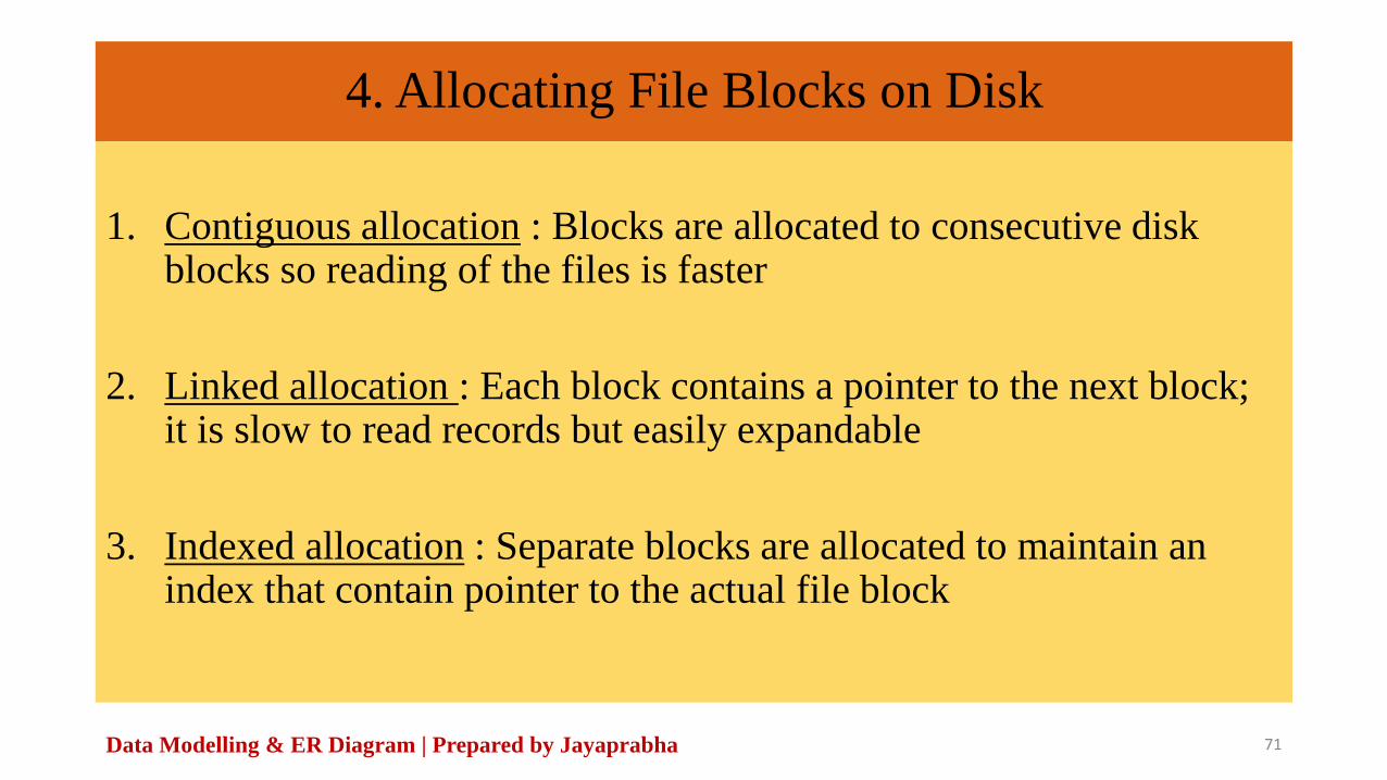
4. Allocating File Blocks on Disk
1. Contiguous allocation : Blocks are allocated to consecutive disk blocks so reading of the files is faster
2. Linked allocation : Each block contains a pointer to the next block; it is slow to read records but easily expandable
3. Indexed allocation : Separate blocks are allocated to maintain an index that contain pointer to the actual file block
Data Modelling & ER Diagram | Prepared by Jayaprabha 71

5. File Headers
1. Contains info about the file
2. The header contains info about :
• Disk address
• Record format (Field Length, Field Type, Separator Char and Record Type {Spanned, Unspanned Record})
• To search a record in the disk, first the blocks are copied to main memory and then the record is searched using “Linear Search” by using address in the file header
Data Modelling & ER Diagram | Prepared by Jayaprabha 72

File Organization – Heap File
• Files with unordered records (Heap files)
Records are placed in the order they are entered
New records are entered at the end of the file
This leads to secondary indices
Inserting new record is very efficient
Data Modelling & ER Diagram | Prepared by Jayaprabha 73
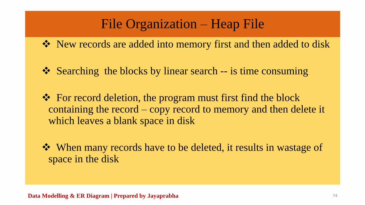
File Organization – Heap File
New records are added into memory first and then added to disk
Searching the blocks by linear search -- is time consuming
For record deletion, the program must first find the block containing the record – copy record to memory and then delete it which leaves a blank space in disk
When many records have to be deleted, it results in wastage of space in the disk
Data Modelling & ER Diagram | Prepared by Jayaprabha 74

File Organization – Heap File
To avoid such wastage, records are not deleted but instead marked for deletion; when there is a periodical reorganization, the marked records are purged and new records are inserted
Spanned or Unspanned org can be used for fixed / variable length records
To sort all records in the file based on certain field, the sorted file is maintained separately
Data Modelling & ER Diagram | Prepared by Jayaprabha 75

Heap file Organization
Data Modelling & ER Diagram | Prepared by Jayaprabha 76

Heap file Organization- using index
Data Modelling & ER Diagram | Prepared by Jayaprabha 77

Sorted file
• Files are placed in a particular order
• So reading/ accessing the files data is fast and easy
• Searching can be done based on some searching key
• Binary search is the technique used for searching a record in sorted file
Data Modelling & ER Diagram | Prepared by Jayaprabha 78

Sort file - insert
• In case a record starting with ‘j’ has to be searched then it uses binary search technique which uses log2(b) formula where b= block
• Inserting a new record is a very tedious task because pushing the other records further down and inserting a new rec at the required place is time consuming
Data Modelling & ER Diagram | Prepared by Jayaprabha 79

Sort file - insert
• To avoid this problem, some free space can be reserved in every block so that a new records can be added into it.
• If the record is too big to be stored in the free space then the rest of the data will move to the overflow area.
• A pointer is used to pointer to the data in the overflow area.
Data Modelling & ER Diagram | Prepared by Jayaprabha 80

Sort file - delete
• Records are not deleted at once but marked for deletion.
•
• During re-organization, the marked records are permanently deleted.
Data Modelling & ER Diagram | Prepared by Jayaprabha 81

Data striping
• Data striping transparently distributes data over multiple disks to make them appear as a single fast, large disk.
• Striping improves the I/O performance by allowing multiple I/Os to be serviced in parallel.
Data Modelling & ER Diagram | Prepared by Jayaprabha 82

RAID
• Redundant Array of Inexpensive/ Independent Disks
• RAID is a storage technology that combines multiple disk drive components into a logical unit for the purposes of data redundancy and performance improvement.
• Data is distributed across the drives in one of several ways, referred to as RAID levels
Data Modelling & ER Diagram | Prepared by Jayaprabha 83

RAID – Redundant Array of Inexpensive/ Redundant Disks
Data Modelling & ER Diagram | Prepared by Jayaprabha 84

RAID
Data Modelling & ER Diagram | Prepared by Jayaprabha 85

Raid 1
Data Modelling & ER Diagram | Prepared by Jayaprabha 86

RAID 2
• A RAID 2 stripes data at the bit (rather than block) level, and uses a Hamming code for error correction.
• The disks are synchronized by the controller to spin at the same angular orientation so it generally cannot service multiple requests simultaneously.
• Extremely high data transfer rates are possible.
Data Modelling & ER Diagram | Prepared by Jayaprabha 87

Parity bit
A parity bit, or check bit is a bit added to the end
of a string of binary code that indicates whether
the number of bits in the string with the value one
is even or odd.
Parity bits are used as the simplest form of error
detecting code.
Data Modelling & ER Diagram | Prepared by Jayaprabha 88

RAID 2
Data Modelling & ER Diagram | Prepared by Jayaprabha 89

RAID 3
• Uses a single parity disk and figures out which disk has failed with a help of a controller
• Used for large volume of storage
• Gives higher data transfer
Data Modelling & ER Diagram | Prepared by Jayaprabha 90

RAID 4
• Uses block level data striping
Data Modelling & ER Diagram | Prepared by Jayaprabha 91

RAID 5
• Used for storing large volume of data
• Uses block level striping
• Distributes data and parity across all disks
• It requires all drives -but atleast one drive must be present to operate.
• Upon failure of a single drive, subsequent reads can be calculated from the distributed parity such that no data is lost.
Data Modelling & ER Diagram | Prepared by Jayaprabha 92

RAID 5
Data Modelling & ER Diagram | Prepared by Jayaprabha 93
RAID 6
• RAID 6 extends RAID 5 by adding an additional parity block; thus it uses block-level striping with two parity blocks distributed across all member disks.
Data Modelling & ER Diagram | Prepared by Jayaprabha 94

RAID 6
Data Modelling & ER Diagram | Prepared by Jayaprabha 95

B Tree
• A B-tree is a method of placing and locating files (called records) in a database
• The B-tree algorithm minimizes the number of times a medium must be accessed to locate a desired record, thereby speeding up the process.
• B-tree is a tree data structure that keeps data sorted and allows searches, sequential access, insertions, and deletions in a very short time.
• The B-tree is a generalization of a binary search tree in that a node can have more than two children
Data Modelling & ER Diagram | Prepared by Jayaprabha 96

Important Questions
• What is a Data model? Explain its different types
• 3 schema architecture
• Centralized architecture
• Buffering of blocks
• Data independence, data abstraction
• Client- server or 3 tier architecture
Data Modelling & ER Diagram | Prepared by Jayaprabha 97