dbkda 2016 proceedings - reutlingen university · vladimir ivancevic, university of novi sad,...

DBKDA 2016

The Eighth International Conference on Advances in Databases, Knowledge, and

Data Applications

ISBN: 978-1-61208-486-2

GraphSM 2016

The Third International Workshop on Large-scale Graph Storage and Management

June 26 - 30, 2016

Lisbon, Portugal

DBKDA 2016 Editors

Friedrich Laux, Reutlingen University, Germany

Andreas Schmidt, Karlsruhe University of Applied Sciences | Karlsruhe Institute of

Technology, Germany

Dimitar Hristovski, University of Ljubljana, Slovenia

1 / 107

DBKDA 2016

Foreword

The Eighth International Conference on Advances in Databases, Knowledge, and DataApplications (DBKDA 2016), held between June 26 - 30, 2016 - Lisbon, Portugal, continued a series ofinternational events covering a large spectrum of topics related to advances in fundamentals ondatabases, evolution of relation between databases and other domains, data base technologies andcontent processing, as well as specifics in applications domains databases.

Advances in different technologies and domains related to databases triggered substantialimprovements for content processing, information indexing, and data, process and knowledge mining.The push came from Web services, artificial intelligence, and agent technologies, as well as from thegeneralization of the XML adoption.

High-speed communications and computations, large storage capacities, and load-balancing fordistributed databases access allow new approaches for content processing with incomplete patterns,advanced ranking algorithms and advanced indexing methods.

Evolution on e-business, ehealth and telemedicine, bioinformatics, finance and marketing,geographical positioning systems put pressure on database communities to push the ‘de facto’ methodsto support new requirements in terms of scalability, privacy, performance, indexing, and heterogeneityof both content and technology.

DBKDA 2016 also featured the following Workshop:- GraphSM 2016: The Third International Workshop on Large-scale Graph Storage and

Management

We take here the opportunity to warmly thank all the members of the DBKDA 2016 TechnicalProgram Committee, as well as the numerous reviewers. The creation of such a high quality conferenceprogram would not have been possible without their involvement. We also kindly thank all the authorswho dedicated much of their time and efforts to contribute to DBKDA 2016. We truly believe that,thanks to all these efforts, the final conference program consisted of top quality contributions.

Also, this event could not have been a reality without the support of many individuals,organizations, and sponsors. We are grateful to the members of the DBKDA 2016 organizing committeefor their help in handling the logistics and for their work to make this professional meeting a success.

We hope that DBKDA 2016 was a successful international forum for the exchange of ideas andresults between academia and industry and for the promotion of progress in the fields of databases,knowledge and data applications.

We are convinced that the participants found the event useful and communications very open.We also hope that Lisbon provided a pleasant environment during the conference and everyone savedsome time for exploring this beautiful city.

DBKDA 2016 Chairs:

Friedrich Laux, Reutlingen University, GermanyAris M. Ouksel, The University of Illinois at Chicago, USASerge Miranda, Université de Nice Sophia Antipolis, France

2 / 107

Andreas Schmidt, Karlsruhe University of Applied Sciences | Karlsruhe Institute of Technology, GermanyMaribel Yasmina Santos, University of Minho, PortugalFilip Zavoral, Charles University Prague, Czech RepublicMaria Del Pilar Angeles, Universidad Nacional Autonoma de Mexico - Del Coyoacan, MexicoDimitar Hristovski, University of Ljubljana, SloveniaChristian Krause, SAP Innovation Center Potsdam, Germany

3 / 107

DBKDA 2016

Committee

DBKDA Advisory Committee

Friedrich Laux, Reutlingen University, GermanyAris M. Ouksel, The University of Illinois at Chicago, USASerge Miranda, Université de Nice Sophia Antipolis, FranceAndreas Schmidt, Karlsruhe University of Applied Sciences | Karlsruhe Institute of Technology, GermanyMaribel Yasmina Santos, University of Minho, PortugalFilip Zavoral, Charles University Prague, Czech RepublicMaria Del Pilar Angeles, Universidad Nacional Autonoma de Mexico - Del Coyoacan, Mexico

DBKDA 2016 Technical Program Committee

Nipun Agarwal, Oracle Corporation, USASuad Alagic, University of Southern Maine, USAAbdullah Albarrak, University of Queensland, AustraliaToshiyuki Amagasa, University of Tsukuba, JapanBernd Amann, Université Pierre et Marie Curie (UPMC) - LIP6, FranceFabrizio Angiulli, University of Calabria, ItalyMasayoshi Aritsugi, Kumamoto University, JapanZeyar Aung, Masdar Institute of Science and Technology, United Arab EmiratesAna Azevedo, Algoritmi R&D Center/University of Minho & Polytechnic Institute of Porto/ISCAP,PortugalGilbert Babin, HEC Montréal, CanadaIlaria Bartolini, University of Bologna, ItalyOrlando Belo, University of Minho, PortugalFadila Bentayeb, University of Lyon 2, FranceArnab Bhattacharya, IIT Kanpur, IndiaZouhaier Brahmia, University of Sfax, TunisiaFrancesco Buccafurri, University Mediterranea of Reggio Calabria, ItalyErik Buchmann, Karlsruhe Institute of Technology (KIT), GermanyMartine Cadot, LORIA-Nancy, FranceRicardo Campos, Polytechnic Institute of Tomar / LIAAD - INESCT TEC Porto, PortugalMichelangelo Ceci, University of Bari, ItalyChin-Chen Chang, Feng Chia University Taiwan, TaiwanChi-Hua Chen, National Chiao Tung University - Taiwan, R.O.C.Qiming Chen, HP Labs - Palo Alto, USADing-Yuan Cheng, National Chiao Tung University, Taiwan , R.O.C.Yangjun Chen, University of Winnipeg, CanadaYung Chang Chi, National Cheng Kung University, TaiwanCamelia Constantin, UPMC, FranceTheodore Dalamagas, ATHENA Research and Innovation Center, GreeceGabriel David, University of Porto, PortugalMaria Del Pilar Angeles, Universidad Nacional Autonoma de Mexico - Del Coyoacan, Mexico

4 / 107

Taoufiq Dkaki, IRIT - Toulouse, FranceCédric du Mouza, CNAM - Paris, FranceGledson Elias, Universidade Federal da Paraiba, BrazilMarkus Endres, University of Augsburg, GermanyBijan Fadaeenia, Islamic Azad University- Hamedan Branch, IranFeroz Farazi, University of Trento, ItalyManuel Filipe Santos, Algoritmi research centre / University of Minho, PortugalSergio Firmenich, CONICET and LIFIA - Facultad de Informática, Universidad Nacional de La Plata,ArgentinaIngrid Fischer, University of Konstanz, GermanyRobert Gottstein, Technische Universität Darmstadt, GermanyMichael Gowanlock, Massachusetts Institute of Technology, Haystack Observatory, USAJerzy Grzymala-Busse, University of Kansas, USADirk Habich, TU Dresden, GermanyPhan Nhat Hai, University of Oregon, USATakahiro Hara, Osaka University, JapanBingsheng He, Nanyang Technological University, SingaporeErik Hoel, Esri, USATobias Hoppe, Ruhr-University of Bochum, GermanyMartin Hoppen, Institute for Man-Machine Interaction - RWTH Aachen University, GermanyWen-Chi Hou, Southern Illinois University at Carbondale, USAHamidah Ibrahim, Universiti Putra Malaysia, MalaysiaDino Ienco, Irstea Montpellier, FranceYasunori Ishihara, Osaka University, JapanVladimir Ivancevic, University of Novi Sad, SerbiaSavnik Iztok, University of Primorska, SloveniaWassim Jaziri, ISIM Sfax, TunisiaSungwon Jung, Sogang University - Seoul, KoreaVana Kalogeraki, Athens University of Economics and Business, GreeceKonstantinos Kalpakis, University of Maryland Baltimore County, USAMehdi Kargar, York University, Toronto, CanadaRajasekar Karthik, Geographic Information Science and Technology Group/Oak Ridge NationalLaboratory, USANhien An Le Khac, University College Dublin, IrelandSadegh Kharazmi, RMIT University - Melbourne, AustraliaPeter Kieseberg, SBA Research, AustriaDaniel Kimmig, Karlsruhe Institute of Technology, GermanyChristian Kop, University of Klagenfurt, AustriaMichal Kratky, VŠB - Technical University of Ostrava, Czech RepublicJens Krueger, Hasso Plattner Institute / University of Potsdam, GermanyBart Kuijpers, Hasselt University, BelgiumFritz Laux, Reutlingen University, GermanyYoonJoon Lee, KAIST, South KoreaCarson Leung, University of Manitoba, CanadaSebastian Link, The University of Auckland, New ZealandChunmei Liu, Howard University, USACorrado Loglisci, University of Bari, ItalyQiang Ma, Kyoto University, Japan

5 / 107

Sebastian Maneth, University of Edinburgh, UKMurali Mani, University of Michigan - Flint, USAGerasimos Marketos, University of Piraeus, GreeceMichele Melchiori, Università degli Studi di Brescia, ItalyErnestina Menasalvas, Universidad Politécnica de Madrid, SpainAntonio Messina, Italian National Research Council - High Performances Computing and NetworkingInstitute, ItalyElisabeth Métais, CEDRIC / CNAM - Paris, FranceCristian Mihaescu, University of Craiova, RomaniaSerge Miranda, Université de Nice Sophia Antipolis, FranceMehran Misaghi, Educational Society of Santa Catarina – Joinville, BrazilMohamed Mkaouar, Sfax, TunisiaJacky Montmain, LGI2P - Ecole des Mines d'Alès, FranceYasuhiko Morimoto, Hiroshima University, JapanFranco Maria Nardini, ISTI-CNR, ItalyKhaled Nagi, Alexandria University, EgyptShin-ichi Ohnishi, Hokkai-Gakuen University, JapanBenoît Otjacques, LIST - Luxembourg Institute of Science and Technology, LuxembourgAris M. Ouksel, The University of Illinois at Chicago, USAGeorge Papastefanatos, Athena Research and Innovation Center, GreeceFrancesco Parisi, University of Calabria, ItalyAlexander Pastwa, Ruhr-Universität Bochum, GermanyDhaval Patel, IIT-Roorkee, SingaporePrzemyslaw Pawluk, York University - Toronto, CanadaBernhard Peischl, Softnet Austria | Institut für Softwaretechnologie | Technische Universität Graz,AustriaAlexander Peter, AOL Data Warehouse, USAAlain Pirotte, University of Louvain (Louvain-la-Neuve), BelgiumPascal Poncelet, LIRMM, FrancePhilippe Pucheral, University of Versailles & INRIA, FranceRicardo Queirós, ESEIG-IPP, PortugalMandar Rahurkar, Yahoo! Labs, USAPraveen R. Rao, University of Missouri-Kansas City, USAPeter Revesz, University of Nebraska-Lincoln, USAMathieu Roche, TETIS, Cirad, FranceMiguel Romero, University of Chile, ChileFlorin Rusu, University of California, Merced, USAGunter Saake, Otto-von-Guericke-University Magdeburg, GermanySatya Sahoo, Case Western Reserve University, USAFatiha Saïs, LRI (CNRS & Paris Sud University), FranceEmanuel Sallinger, University of Oxford, UKAbhishek Sanwaliya, Indian Institute of Technology - Kanpur, IndiaIsmael Sanz, Universitat Jaume I - Castelló, SpainMaria Luisa Sapino, Università degli Studi di Torino, ItalyM. Saravanan, Ericsson India Pvt. Ltd -Tamil Nadu, IndiaIdrissa Sarr, Université Cheikh Anta Diop, SenegalNajla Sassi Jaziri, ISSAT Mahdia, TunisiaAndreas Schmidt, Karlsruhe University of Applied Sciences | Karlsruhe Institute of Technology, Germany

6 / 107

Yong Shi, Kennesaw State University, USADamires Souza, Federal Institute of Education, Science and Technology of Paraiba (IFPB), BrazilLubomir Stanchev, California Polytechnic State University, San Luis Obispo, USAAhmad Taleb, Najran University, Saudi ArabiaTony Tan, National Taiwan University, TaiwanMaguelonne Teisseire, Irstea - UMR TETIS, FranceTelesphore Tiendrebeogo, Polytechnic University of Bobo-Dioulasso, Burkina FasoGabriele Tolomei, CNR, ItalyJose Torres-Jimenez, CINVESTAV 3C, MexicoNicolas Travers, CNAM-Paris, FranceThomas Triplet, Computer Research Institute of Montreal (CRIM), CanadaMarina Tropmann-Frick, Christian-Albrechts-University of Kiel, GermanyRobert Ulbricht, Robotron Datenbank-Software GmbH, GermanyMarian Vajtersic, University of Salzburg, AustriaMaurice van Keulen, University of Twente, NetherlandsGenoveva Vargas, Solar | CNRS | LIG-LAFMIA, FranceMarcio Victorino, University of Brasília, BrazilFan Wang, Microsoft Corporation - Bellevue, USAZhihui Wang, Dalian University of Technology, ChinaKesheng (John) Wu, Lawrence Berkeley National Laboratory, USAGuandong Xu, Victoria University, AustraliaMaribel Yasmina Santos, University of Minho, PortugalJin Soung Yoo, Indiana University-Purdue University - Fort Wayne, USAFeng Yu, Youngstown State University, USAFilip Zavoral , Charles University Prague, Czech RepublicWei Zhang, Amazon.com, USAJiakui Zhao, State Grid Information & Telecommunication Gruop, China

GraphSM 2016 Advisory Committee

Dimitar Hristovski, University of Ljubljana, SloveniaAndreas Schmidt, Karlsruhe University of Applied Sciences & Karlsruhe Institute of Technology, GermanyChristian Krause, SAP Innovation Center Potsdam, Germany

GraphSM 2016 Technical Program Committee

Khaled Ammar, University of Waterloo, CanadaBlaz Fortuna, Jozef Stefan Institute, SloveniaHolger Giese, Hasso-Plattner-Institut, GermanyDimitar Hristovski, University of Ljubljana, SloveniaYasunori Ishihara, Osaka University, JapanChristian Krause, SAP Innovation Center Potsdam, GermanyDejan Lavbic, University of Ljubljana, SloveniaKhaled Nagi, Alexandria University, EgyptElena Ravve, Ort-Braude College - Karmiel, IsraelAndreas Schmidt, Karlsruhe University of Applied Sciences & Karlsruhe Institute of Technology, GermanyJim Webber, Neo Technology, USATatjana Wezler, University of Maribor, Slovenia

7 / 107

Kokou Yetongnon, Université de Bourgogne, FranceAlbert Zündorf, Kassel University, Germany

8 / 107

Copyright Information

For your reference, this is the text governing the copyright release for material published by IARIA.

The copyright release is a transfer of publication rights, which allows IARIA and its partners to drive the

dissemination of the published material. This allows IARIA to give articles increased visibility via

distribution, inclusion in libraries, and arrangements for submission to indexes.

I, the undersigned, declare that the article is original, and that I represent the authors of this article in

the copyright release matters. If this work has been done as work-for-hire, I have obtained all necessary

clearances to execute a copyright release. I hereby irrevocably transfer exclusive copyright for this

material to IARIA. I give IARIA permission or reproduce the work in any media format such as, but not

limited to, print, digital, or electronic. I give IARIA permission to distribute the materials without

restriction to any institutions or individuals. I give IARIA permission to submit the work for inclusion in

article repositories as IARIA sees fit.

I, the undersigned, declare that to the best of my knowledge, the article is does not contain libelous or

otherwise unlawful contents or invading the right of privacy or infringing on a proprietary right.

Following the copyright release, any circulated version of the article must bear the copyright notice and

any header and footer information that IARIA applies to the published article.

IARIA grants royalty-free permission to the authors to disseminate the work, under the above

provisions, for any academic, commercial, or industrial use. IARIA grants royalty-free permission to any

individuals or institutions to make the article available electronically, online, or in print.

IARIA acknowledges that rights to any algorithm, process, procedure, apparatus, or articles of

manufacture remain with the authors and their employers.

I, the undersigned, understand that IARIA will not be liable, in contract, tort (including, without

limitation, negligence), pre-contract or other representations (other than fraudulent

misrepresentations) or otherwise in connection with the publication of my work.

Exception to the above is made for work-for-hire performed while employed by the government. In that

case, copyright to the material remains with the said government. The rightful owners (authors and

government entity) grant unlimited and unrestricted permission to IARIA, IARIA's contractors, and

IARIA's partners to further distribute the work.

9 / 107

Table of Contents

Object-Relational Mapping in 3D SimulationAnn-Marie Stapelbroek, Martin Hoppen, and Juergen Rossmann

1

A Text Analyser of Crowdsourced Online Sources for Knowledge DiscoveryIoannis Markou and Efi Papatheocharous

8

A Novel Reduced Representation Methodology for Provenance DataMehmet Gungoren and Mehmet Siddik Aktas

15

An Efficient Algorithm for Read Matching in DNA DatabasesYangjun Chen, Yujia Wu, and Jiuyong Xie

23

A Simplified Database Pattern for the Microservice ArchitectureAntonio Messina, Riccardo Rizzo, Pietro Storniolo, and Alfonso Urso

35

Multidimensional Structures for Field Based Data. A Review of ModelsTaher Omran Ahmed

41

Some Heuristic Approaches for Reducing Energy Consumption on Database SystemsMiguel Guimaraes, Joao Saraiva, and Orlando Belo

49

A Framework for Semantic Web of Patent InformationYung Chang Chi, Hei Chia Wang, and Ying Maw Teng

54

A Comparison of Two MLEM2 Rule Induction Algorithms Applied to Data with Many Missing Attribute ValuesPatrick G. Clark, Cheng Gao, and Jerzy W. Grzymala-Busse

60

A Distributed Algorithm For Graph Edit DistanceZeina Abu-Aisheh, Romain Raveaux, Jean-Yves Ramel, and Patrick Martineau

66

Discovering the Most Dominant Nodes in Frequent SubgraphsFarah Chanchary, Herna Viktor, and Anil Maheshwari

72

Managing 3D Simulation Models with the Graph Database Neo4jMartin Hoppen, Juergen Rossmann, and Sebastian Hiester

78

Subgraph Similarity Search in Large GraphsKanigalpula Samanvi and Naveen Sivadasan

84

Implementing Semantics-Based Cross-domain Collaboration Recommendation in Biomedicine with a Graph 94

1 / 2 10 / 107

DatabaseDimitar Hristovski, Andrej Kastrin, and Thomas C. Rindflesch

Powered by TCPDF (www.tcpdf.org)

2 / 2 11 / 107

Object-Relational Mapping in 3D Simulation

Ann-Marie Stapelbroek,Martin Hoppen

and Juergen Rossmann

Institute for Man-Machine InteractionRWTH Aachen UniversityD-52074 Aachen, Germany

Email: [email protected] {hoppen,rossmann}@mmi.rwth-aachen.de

Abstract—Usually, 3D simulation models are based on complexobject-oriented structures. To master this complexity, databasesshould be used. However, existing approaches for 3D modeldata management are not sufficiently comprehensive and flexible.Thus, we develop an approach based on the relational datamodel as the most widespread database paradigm. To successfullycombine an object-oriented 3D simulation system and a relationaldatabase management system, a mapping has to be definedbridging the differences in between. These are summarized as theobject-relational impedance mismatch. Theoretical foundationsof object-relational mapping are researched and existing, semi-automatic object-relational mappers are evaluated. As it turnsout, existing mappers are not applicable in the presented case.Therefore, a new object-relational mapper is developed based onthe utilized simulation system’s meta information system. Keyaspects of the developed approach are a necessary adaptationof the theoretical object-relational mapping strategies, databaseindependence in conjunction with data type mapping, schemamapping by schema synchronization, and strategies for savingand loading model data as well as for change tracking. Thedeveloped prototype is evaluated using two exemplary simulationmodels from the fields of industrial automation and spacerobotics.

Keywords–Object-Oriented 3D Simulation System; RelationalData Model; Relational Database Management System; Object-Relational Mapper; Object-Relational Mapping; Object-RelationalImpedance Mismatch.

I. INTRODUCTION

3D simulation systems are used in different areas likespace robotics and industrial automation to derive properties –especially, spatial properties – of a planned or existing system’sbehavior. Usually, 3D simulations are based on complex andextensive models. Therefore, databases are appropriate for datamanagement to master the complex object-oriented structuresof 3D simulation models and to make simulation states persis-tent [1]. As a result, different simulation runs can be recordedand analyzed [2]. In comparison with flat file storage, the usageof databases has key advantages, in particular, if data indepen-dence, multi-user synchronization, data integrity, data security,reliability, efficient data access and scalability are required [3].However, existing approaches for 3D model data managementusing databases are not sufficiently comprehensive and flexible,motivating the development of a new approach.

The most widespread database paradigm is the relationaldata model. If relational databases should be used as apersistence layer for object-oriented 3D simulation systems,

a mapping has to be defined bridging the differences be-tween both paradigms. These differences are summarized asthe object-relational impedance mismatch. The term object-relational mapping (OR mapping) describes the process ofmapping the objects of an application (here, a 3D simulationsystem) to table entries of a relational database and vice versa.A manual mapping between the object-oriented concept andthe relational database model is complex and error-prone sothat object-relational mappers (OR mappers) are used. AnOR mapper is a tool that builds a translation layer betweenapplication logic and relational database to perform a semi-automatic object-relational mapping.

Figure 1. OR mapping for a 3D simulation system with an object-orientedruntime database (data: [4]).

In this paper, we present an OR mapper for 3D simulationsystems with an object-oriented runtime database and a metainformation system, see Figure 1. The work was conducted asa student project and is based on our previous work [1] [2].A prototypical implementation is based on the 3D simulationsystem VEROSIM [5] and PostgreSQL [6] as a relationaldatabase management system (RDBMS). However, the under-lying approach itself provides database independence allowingthe usage of other RDBMSs. A key aspect of the presentedOR mapping is the schema mapping that is build during aschema synchronization (based on [2]). The introduced conceptconsiders both forward and reverse mapping. Furthermore, theOR mapper supports change tracking and resynchronization ofchanges. The OR mapper provides an eager and a lazy loadingstrategy. The prototype is evaluated using simulation modelsfor industrial automation and space robotics (Figure 11).

The rest of this paper is organized as follows: In the nextsection, similar applications with a 3D context that integratedatabase technology are analyzed. Section III contains a shortsummary regarding the theoretical principals of OR mapping

1Copyright (c) IARIA, 2016. ISBN: 978-1-61208-486-2

DBKDA 2016 : The Eighth International Conference on Advances in Databases, Knowledge, and Data Applications

12 / 107

and Section IV introduces the utilized 3D simulation systemVEROSIM and evaluates existing OR mappers. Subsequently,the newly developed concept for OR mapping is introduced inSection V and evaluated in Section VI. Finally, the paper isconcluded in Section VII.

II. RELATED WORK

In general, many applications with a 3D context havedata management requirements similar to 3D simulation. Yet,the use of database technology is not widespread and filesare still predominant. When databases are utilized at all, inmany scenarios, they are used to store additional information(meta information, documents, films, positions, hierarchicalstructure . . . ) on scene objects or parts [7] [8] [9] [10] [11][12] [13]. Yet, we need to manage the 3D model itself toobtain all the benefits from using database technology. Anotherimportant aspect for 3D simulation is arbitrary applicationschema support to be able to work with native data andavoid friction loss due to conversions. Many systems usea generic (scene-graph-like) geometric model, in most caseswith attributes [7] [14] [15] [16] [17]. In such scenarios,schema flexibility can be achieved to a certain extent byproviding import (and export) to different file formats [15][18] [19] [20]. Some approaches support different or flexibleschemata. For example in [14], schema alteration is realizedby adding attributes to generic base objects. Other systemssupport a selection of different static [15] or dynamic [16][21] schemata. However, most approaches focus on a specificfield of application, thus, requiring and supporting only acorresponding fixed schema [22] [23] [24]. While Product DataManagement (PDM) systems [8] [9] or similar file vaultingapproaches for 3D data [25] [26] [27] in principle supportarbitrary schemata they are not explicitly reflected within thedatabase schema due to their ”black box integration” approach.Most scenarios provide a distributed architecture in terms ofmultiuser support, a client-server model, or access controland rights management. However, only some build it on aDistributed Database (DDB)-like approach [21] [28] [17] withclient-side databases. The latter is favorable for 3D simulation,e.g., to provide schema flexibility or a query interface on client-side, as well.

Altogether, while there are many existing approaches to usedatabase technology in applications with a 3D context, noneof them provides a comprehensive and flexible solution thatfulfills all the requirements for 3D simulation.

III. OBJECT-RELATIONAL MAPPING

Some RDBMSs provide additional object-relational fea-tures. For example, PostgreSQL supports some object-orientedextensions like user defined types or inheritance. However,these features are not provided uniformly by all RDBMSscontradicting the desired database independence. Therefore,the OR mapping is realized with standard relational conceptsonly.

There are several references in literature dealing with thedifferences between object-oriented concepts and the relationaldata model. To solve the object-relational impedance mismatchand successfully generate an OR mapper, it is important toconsider the properties of both paradigms and the consequentproblems. For example, one main idea of object-orientationis inheritance [29]. However, the relational data model does

not feature any comparable concept. Thus, rules have to bedefined how inheritance can be mapped onto table structures.Further differences between both paradigms that contribute tothe object-relational impedance mismatch are polymorphism,data types, identity, data encapsulation, and relationships.

The following subsections summarize the state-of-the-artof theoretical mapping strategies for inheritance, relationshipsand polymorphism.

A. InheritanceThe approaches to map objects onto tables differ in to

how many tables one object is mapped. Most authors namethree standard mapping strategies for inheritance. They areillustrated in Figure 3 regarding the exemplary inheritancehierarchy from Figure 2.

Figure 2. Exemplary inheritance hierarchy (adapted from [30, p. 62f]).

The first strategy is named Single Table Inheritance [30]and maps all classes of one inheritance hierarchy to one table,see Figure 3(a). A discriminator field is used to denote the typeof each tuple [31]. An advantage is that all data is stored in onetable preventing joins and allowing simple updates [30, p. 63].Unfortunately, this strategy leads to a total denormalization,which is contrary to the concept of relational databases [31].

(a) Single TableInheritance.

(b) Concrete Ta-ble Inheritance.

(c) Class TableInheritance.

Figure 3. Standard mapping strategies for inheritance (adapted from [30, p.62f]).

The Concrete Table Inheritance [30] strategy maps eachconcrete class to one table, see Figure 3(b). This mappingrequires only few joins to retrieve all data for one object.A disadvantage is that schema changes in base classes arelaborious and error-prone. [30, p. 62f]

The third standard mapping strategy for inheritance isnamed Class Table Inheritance [30] and uses one table for



13 / 107

each class of the hierarchy, see Figure 3(c). It is the easiestapproach to map objects onto tables [30, p. 62] and uses anormalized schema [31]. However, due to the use of foreignkeys, this approach realizes an is-a relationship as a has-arelationship [31]. Thus, multiple joins are necessary if all dataof one object is required. This aspect can have an effect onperformance. [30, p. 62f] [32, p. 7]

Another possibility to map objects onto tables not men-tioned in every reference on OR mapping is the genericapproach [33]. It differs from the strategies mentioned above asit has no predefined structure. Figure 4 shows an exemplaryset-up, which can be extended as required. The approach isparticularly suitable for small amounts of data because it mapsone object to multiple tables. It is advantageous if a highlyflexible structure is required. Due to the generic table structure,elements can easily be added or rearranged. [33]

Figure 4. Map classes to generic table structure (adapted from [33, chapter2.4]).

In conclusion, there is no single perfect approach to mapobjects onto tables yielding an optimal result in all situations.Instead, a decision has to be made from case to case dependingon the most important properties. For this purpose, the threestandard mapping strategies for inheritance can also be com-bined, however, to the disadvantage of more complexity. [30,p. 63]

B. RelationshipsIn contrast to relationships between two objects, which can

be unidirectional, relationships between tables in a relationaldatabase are always bidirectional. In unidirectional relation-ships, associated objects do not know if and when they are ref-erenced by another object [32]. Due to the mandatory mappingof unidirectional onto bidirectional relationships, informationhiding cannot be preserved regardless of the relationship’scardinality, i.e., 1:1 (one-to-one), 1:n (one-to-many) or n:m(many-to-many) relationships.

1:1 relationships can simply be mapped onto tables usinga foreign key. To map 1:n relationships, structures have tobe reversed. [33] [30, p. 58f] In case of n:m relationships,additional tables are mandatory: A so-called association tableis used to link the participating tables. [33] [30, p. 60] It isalso possible to map an n:m relationship using multiple foreignkeys in both tables if constant values for n and m are known.[33]

Several references describe the aforementioned mappingstrategies for relationships. Besides, [34] describes an approachusing an additional table regardless of the cardinality. Thus,

objects can be mapped onto tables regardless of their relation-ships. Following [34], one disadvantage of the aforementionedapproaches is the violation of the object-oriented principle ofinformation hiding and abstraction. Furthermore, tables arecluttered by foreign key columns which reduce maintainabilityand performance. The authors prove (by a performance test)that their own approach shows no performance degradation.[34, p. 1446f]

C. PolymorphismPolymorphism is an essential concept in object-orientation.

However, relational databases do not have any feature toreference entries of different tables by one foreign key column.The target table and column have to be explicitly definedfor each foreign key constraint. It is not possible to definea foreign key that references more than one table [35, p. 89].Thus, a mapping is required to map polymorphic associationsonto a relational database. Following [35], [36], there are threemapping approaches for polymorphic associations.

The first approach is named Exclusive Arcs and usesa separate foreign key column for each table that can bereferenced by the polymorphic association, see Figure 5. Thisapproach requires NULL values for foreign key columns. Foreach tuple, at most one of the foreign key columns may beunequal to NULL. Due to foreign key constraints, referentialintegrity can be ensured. However, the administrative effort forthe aforementioned NULL rule is high. An advantage of thisapproach is that queries can easily be formulated.

Figure 5. Mapping of polymorphic associations using Exclusive Arcs.

Another approach is named Reverse the Relationship andis shown in Figure 6. It uses an intermediate table with twoforeign key columns like the aforementioned approach for n:mrelationships. Such an intermediate table has to be definedfor each possible type (table) that can be referenced by thepolymorphic association. [35], [36] The application has toensure that only one entry of all subordinate tables is assignedto the entry of the superordinate table. [35, p. 96ff]

Figure 6. Mapping of polymorphic associations using Reverse theRelationship.

The third approach uses a super table (or “base table”)and is named Base Parent Table. It is based on the basic ideaof polymorphism where subtypes can be referenced using acommon, often abstract supertype. In most cases, these super-types themselves are not mapped to the relational database.



14 / 107

The strategy uses a table to represent a supertype for all itssubtypes’ tables as shown in Figure 7.

Figure 7. Mapping of polymorphic associations using Base Parent Table.

Such a base table only consists of one column containinga primary key value. The assigned subordinate entry has thesame primary key value as the entry of the base table. Thus,an unambiguous assignment is possible. This approach has thebig advantage that base tables do not have to be consideredin queries. They are only used to ensure referential integrity.[35, p. 100ff]

IV. EXISTING SOLUTIONS

For a long time, differences between both the object-oriented and relational paradigm were bridged by simpleprotocols like Java Database Connectivity (JDBC) and OpenDatabase Connectivity (ODBC), which provide a general in-terface to different relational databases. These interfaces havethe disadvantage that the programmer itself is responsible fordata exchange between objects and tables. Due to the mixingof SQL statements and object-oriented commands, this usuallyleads to complex program code that is not easily maintained.[31]

OR mappers are used to realize a simpler and smartermapping between objects and table entries on the one sideand a clear separation between the object-oriented and rela-tional layer on the other side. Thus, the application can bedeveloped independently of the mapping and the database. Asa consequence, different development teams can be deployed.[31]

There are several tools for OR mapping with differentfeatures and documentation. Examples are Hibernate (Java),NHibernate (.NET), ADO.NET Entity Framework (.NET),LINQ to SQL (.NET), Doctrine (PHP), ODB (C++), LiteSQL(C++), and QxOrm (C++). Not every existing mapper featuresall three standard mapping strategies for inheritance. Anothermain difference is how the mapping approach can be specified.In particular, OR mappers like Hibernate [37] and NHibernate[38] recommend an XML-based mapping while mappers likeODB [39] and QxORM [40] recommend the opposite.

The applicability of an OR mapper depends on the utilizedapplication. In the presented scenario, this is the 3D simulationsystem VEROSIM, which is subsequently introduced beforepresenting the evaluation of existing OR mappers.

VEROSIM uses an in-memory runtime database calledVersatile Simulation Database (VSD) for its internal datamanagement. It is an object-oriented graph database providingthe means to describe structure as well as behavior of asimulation model. Besides interfaces for data manipulation, itprovides a change notification mechanism for updates, insertsand deletes. In VSD, objects are called instances and theirclasses are described by so-called meta instances representing

the meta information system of VSD. Instances can haveproperties for simple values (e.g., integers or strings) or forreferencing other instances – either a single target (1:1) or alist of targets (1:n). During runtime, instances can be identifiedby a unique id. VEROSIM and VSD are implemented in C++.[5]

Thus, an OR mapping is required that maps data of aruntime database like VSD onto a relational database. Noneof the existing OR mappers support a direct mapping of aruntime database’s meta information system. They only mapobject-oriented classes and objects of a specific programminglanguage. Similarly, the approach used in our previous work [2]maps a relational database to a generic object interface that issubsequently mapped to VSD. Thus, if one of these mappers isused, a second mapping is required to map between the metainformation system and the object-oriented layer of the ORmapper.

Based on meta instances, any VSD instance can be clas-sified during runtime. This is a key advantage for the ORmapping with regard to the generation and maintenance ofall mappings. Thus, the decision was made to develop a newOR mapper. This allows the OR mapping to be tailored to therequirements of runtime simulation databases like VSD.

V. OBJECT-RELATIONAL MAPPER FOR 3D SIMULATIONSYSTEMS

A basic decision criterion for OR mapping is the def-inition of the database schema. Given an existing object-oriented schema, forward mapping is used to derive a relationaldatabase schema. In contrast, if the initial situation is a givenrelational database schema, reverse mapping is used to derivean object-oriented schema. As already mentioned, databaseindependence is a key aspect of OR mapping. In reversemapping, this aspect is omitted as a specific database schemaof a particular RDBMS is used as the basis for the mapping.[31] The focus of the presented OR mapper is forward mappingto map existing model data of the 3D simulation system ontoan arbitrary relational database. Nevertheless, reverse mappingis supported in the concept as well to use the 3D simulationsystem for other existing databases (see the upper path inFigure 8).

The designed forward mapping of the presented OR map-per is briefly described in the following paragraph and theoverall structure of the OR mapper is shown in Figure 8.

First of all, the database schema has to be generated to beable to store object-oriented simulation data in the relationaldatabase. Subsequently, a schema synchronization defines aschema mapping between the object-oriented and the relationalschema. More details on this are given in [2]. The schemamapping defines which meta instance is mapped to whichtable. Based on this mapping, initial simulation model datacan be stored. Generate Schema Based on Meta Informationand Export Model Data in Database are performed only onceand can be seen as the initialization of the OR mapping.Subsequently, model data can be loaded from the relationaldatabase and updated within the simulation database. A changetracking mechanism keeps track of changes within the simu-lation database and allows for their resynchronization to therelational database.



15 / 107

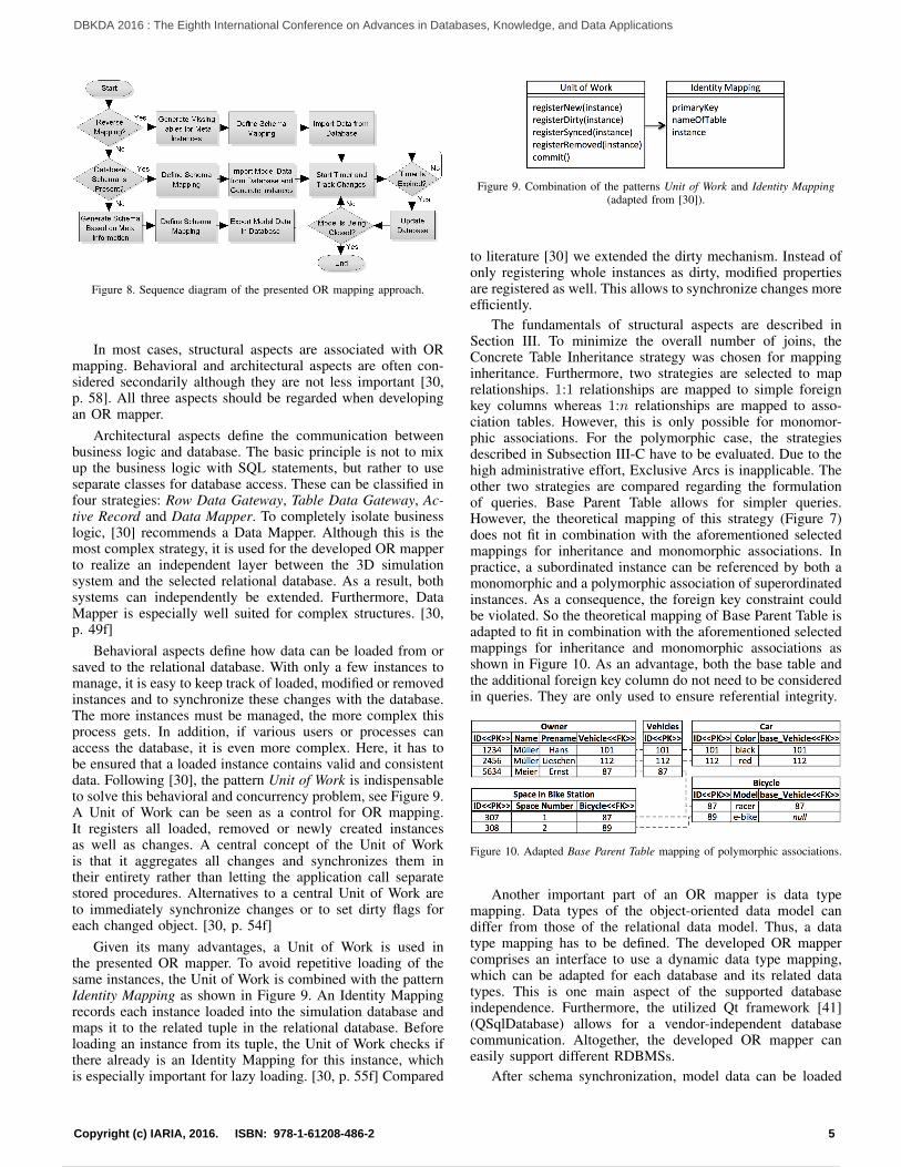
Figure 8. Sequence diagram of the presented OR mapping approach.

In most cases, structural aspects are associated with ORmapping. Behavioral and architectural aspects are often con-sidered secondarily although they are not less important [30,p. 58]. All three aspects should be regarded when developingan OR mapper.

Architectural aspects define the communication betweenbusiness logic and database. The basic principle is not to mixup the business logic with SQL statements, but rather to useseparate classes for database access. These can be classified infour strategies: Row Data Gateway, Table Data Gateway, Ac-tive Record and Data Mapper. To completely isolate businesslogic, [30] recommends a Data Mapper. Although this is themost complex strategy, it is used for the developed OR mapperto realize an independent layer between the 3D simulationsystem and the selected relational database. As a result, bothsystems can independently be extended. Furthermore, DataMapper is especially well suited for complex structures. [30,p. 49f]

Behavioral aspects define how data can be loaded from orsaved to the relational database. With only a few instances tomanage, it is easy to keep track of loaded, modified or removedinstances and to synchronize these changes with the database.The more instances must be managed, the more complex thisprocess gets. In addition, if various users or processes canaccess the database, it is even more complex. Here, it has tobe ensured that a loaded instance contains valid and consistentdata. Following [30], the pattern Unit of Work is indispensableto solve this behavioral and concurrency problem, see Figure 9.A Unit of Work can be seen as a control for OR mapping.It registers all loaded, removed or newly created instancesas well as changes. A central concept of the Unit of Workis that it aggregates all changes and synchronizes them intheir entirety rather than letting the application call separatestored procedures. Alternatives to a central Unit of Work areto immediately synchronize changes or to set dirty flags foreach changed object. [30, p. 54f]

Given its many advantages, a Unit of Work is used inthe presented OR mapper. To avoid repetitive loading of thesame instances, the Unit of Work is combined with the patternIdentity Mapping as shown in Figure 9. An Identity Mappingrecords each instance loaded into the simulation database andmaps it to the related tuple in the relational database. Beforeloading an instance from its tuple, the Unit of Work checks ifthere already is an Identity Mapping for this instance, whichis especially important for lazy loading. [30, p. 55f] Compared

Figure 9. Combination of the patterns Unit of Work and Identity Mapping(adapted from [30]).

to literature [30] we extended the dirty mechanism. Instead ofonly registering whole instances as dirty, modified propertiesare registered as well. This allows to synchronize changes moreefficiently.

The fundamentals of structural aspects are described inSection III. To minimize the overall number of joins, theConcrete Table Inheritance strategy was chosen for mappinginheritance. Furthermore, two strategies are selected to maprelationships. 1:1 relationships are mapped to simple foreignkey columns whereas 1:n relationships are mapped to asso-ciation tables. However, this is only possible for monomor-phic associations. For the polymorphic case, the strategiesdescribed in Subsection III-C have to be evaluated. Due to thehigh administrative effort, Exclusive Arcs is inapplicable. Theother two strategies are compared regarding the formulationof queries. Base Parent Table allows for simpler queries.However, the theoretical mapping of this strategy (Figure 7)does not fit in combination with the aforementioned selectedmappings for inheritance and monomorphic associations. Inpractice, a subordinated instance can be referenced by both amonomorphic and a polymorphic association of superordinatedinstances. As a consequence, the foreign key constraint couldbe violated. So the theoretical mapping of Base Parent Table isadapted to fit in combination with the aforementioned selectedmappings for inheritance and monomorphic associations asshown in Figure 10. As an advantage, both the base table andthe additional foreign key column do not need to be consideredin queries. They are only used to ensure referential integrity.

Figure 10. Adapted Base Parent Table mapping of polymorphic associations.

Another important part of an OR mapper is data typemapping. Data types of the object-oriented data model candiffer from those of the relational data model. Thus, a datatype mapping has to be defined. The developed OR mappercomprises an interface to use a dynamic data type mapping,which can be adapted for each database and its related datatypes. This is one main aspect of the supported databaseindependence. Furthermore, the utilized Qt framework [41](QSqlDatabase) allows for a vendor-independent databasecommunication. Altogether, the developed OR mapper caneasily support different RDBMSs.

After schema synchronization, model data can be loaded



16 / 107

from the relational database populating the simulation databasewith corresponding instances. A so-called eager loading strat-egy is used to immediately load and generate all modelinstances. The Unit of Work generates an identity mapping foreach loaded instance. This provides an unambiguous mappingbetween each loaded instance and the corresponding tuple inthe relational database. Furthermore, a so-called lazy loadingstrategy is specified for selectively loading model data fromthe database. It is based on the ghost strategy presented in [30,p. 227ff]. Here, typically necessary information, like primarykey and table name, is determined for all tuples from alltables regardless whether the instance is loaded or not. Ghostinstances are generated containing only this partially loadeddata. [30, p. 227ff] The presented OR mapper uses a GhostIdentity Mapping (Figure 9). The advantage of this modifiedapproach is that only “complete” instances are present in the3D simulation system’s runtime database.

VI. APPLICATION

As mentioned before, schema generation and synchroniza-tion work independently of the selected simulation model.All required structures are defined during schema generation.In the evaluated configuration of the 3D simulation systemVEROSIM, 910 tables, 1, 222 foreign key columns, and 2, 456association tables are generated to map all meta instances and1:1 as well as 1:n relationships. The schema generation takesabout 200 seconds on a local PostgreSQL 9.4 installation.The required schema mapping is built up during schemasynchronization and takes about 2.7 seconds.

Due to its flexibility, the OR mapper can be used forany simulation model. The prototype is evaluated using twoexemplary models from two different fields of application:industrial automation and space robotics. Given the currentfunctional range of the presented prototype, further tests donot appear to provide any additional insights.

Figure 11(a) shows the first model from the field of indus-trial robotics. The robot model contains only a few objects sothat only 173 primary keys have to be generated to map allobjects to table entries. It takes about 0.43 seconds to store thewhole robot into the relational database and about 4.7 secondsto load it.

(a) Industrial robot simulationmodel.

(b) Modular satellite simulationmodel (data: [4]).

Figure 11. Evaluated simulation models.

The second model (Figure 11(b)) is a modular satellite.In comparison, it contains much more objects so that 19, 463primary keys are generated to map all objects to table entries.In this case, it takes about 22 seconds to store all objects of

the satellite and about 7.1 seconds to load all of them fromthe relational database.

As mentioned in Section IV, a comparable interface toexisting ORM solutions would be less efficient as well asmore complex and time-consuming to realize due to thenecessary second mapping. Thus, we refrain from performingsuch comparisons.

VII. SUMMARY, CONCLUSION AND FUTURE WORK

In contrast to flat files, database technology provides manyadvantages for managing 3D simulation models. However,existing approaches for database integration into applicationswith a 3D context do not provide a sufficiently comprehensiveand flexible solution. Given the prevalence of relational DBMSand the preferred object-oriented modeling of 3D simulationmodels, an OR mapping approach is recommended. Usingexisting ORM solutions (including our previous work [2]), anintermediate layer cannot be avoided. Thus, in this work, wedevelop a direct OR mapping approach.

The presented OR mapper allows a flexible and genericmapping between an object-oriented runtime simulationdatabase and a relational database. It is based on the metainformation system so that an OR mapping can be performedfor arbitrary simulation models. The mapper detects schemachanges, i.e., new or modified meta instances, and automati-cally adapts the used mapping without the need for a manualdefinition of persistent elements. Hence, compared to existingOR mappers, a complex and error-prone manual maintenanceof the defined mapping can be omitted. The presented ORmapper separates the 3D simulation system and the usedrelational database so that business logic is not mixed withSQL statements. As a result, the 3D simulation system canbe developed independently from data storage. Future projectscan profit by time saving as they do not have to realizepersistent data storage separately. Following [42, p. 525], theprogramming effort for storing objects in relational databasesaccounts for 20-30% of the total project effort. Finally, thepresented OR mapping is successfully evaluated using twosimulation models from two different fields of application(industrial automation and space robotics).

In future, data type mapping can be extended by morespecialized data types and further RDBMSs can be combinedwith the prototype. Furthermore, the currently generated struc-tures within the relational database do not contain explicitinformation on the inheritance relationships as they are notneeded by the simulation system itself (they can be retrievedfrom its meta information system). However, to allow thirdparty applications to interpret the data, inheritance structureswould be of interest. Another aspect to investigate is themapping of queries and operations. For the former, an object-based query language meeting VSD’s demands, e.g., XQueryor (a variation of) Java Persistence Query Language (JPQL)or Hibernate Query Language (HQL), needs to be mapped toproper SQL queries. Further performance optimizations and,with an extended functional range of the mapper, evaluationsbeyond the results from the student project could be performed,as well. Finally, we could examine further applications, e.g.,from other fields like forestry.



17 / 107

REFERENCES[1] M. Hoppen and J. Rossmann, “A Database Synchronization Approach

for 3D Simulation Systems,” in DBKDA 2014,The 6th InternationalConference on Advances in Databases, Knowledge, and Data Applica-tions, A. Schmidt, K. Nitta, and J. S. Iztok Savnik, Eds., Chamonix,France, 2014, pp. 84–91.

[2] M. Hoppen, M. Schluse, J. Rossmann, and B. Weitzig, “Database-Driven Distributed 3D Simulation,” in Proceedings of the 2012 WinterSimulation Conference, 2012, pp. 1–12.

[3] A. Kemper and A. Eickler, Database Systems – An Introduction (orig.:Datenbanksysteme–Eine Einfuhrung), 9th ed. Munchen: OldenbourgVerlag, 2013.

[4] J. Weise et al., “An Intelligent Building Blocks Concept for On-Orbit-Satellite Servcing,” in Proceedings of International Symposium onArtificial Intelligence, Robotics and Automation in Space (i-SAIRAS),2012, pp. 1–8.

[5] J. Roßmann, M. Schluse, C. Schlette, and R. Waspe, “A New Ap-proach to 3D Simulation Technology as Enabling Technology foreROBOTICS,” in 1st International Simulation Tools Conference &EXPO 2013, SIMEX’2013, 2013, pp. 39–46.

[6] The PostgreSQL Global Development Group, “PostgreSQL: About,”2015, URL: http://www.postgresql.org/about/ [retrieved: May, 2016].

[7] B. Damer et al., “Data-Driven Virtual Environment Assembly andOperation,” in Virtual Ironbird Workshop, 2004, p. 1.

[8] U. Sendler, The PLM Compendium: Reference book of Product Life-cycle Management (orig.: Das PLM-Kompendium: Referenzbuch desProdukt-Lebenszyklus-Managements). Berlin: Springer, 2009.

[9] Verein Deutscher Ingenieure (VDI), “VDI 2219 - Information technol-ogy in product development Introduction and economics of EDM/PDMSystems (Issue German/English),” Dusseldorf, 2002.

[10] Y. Zhao et al., “The research and development of 3D urban geographicinformation system with Unity3D,” in Geoinformatics (GEOINFOR-MATICS), 2013 21st International Conference on, 2013, pp. 1–4.

[11] D. Pacheco and S. Wierenga, “Spatializing experience: a frameworkfor the geolocalization, visualization and exploration of historical datausing VR/AR technologies,” in Proceedings of the 2014 Virtual RealityInternational Conference, 2014.

[12] A. Martina and A. Bottino, “Using Virtual Environments as a Visual In-terface for Accessing Cultural Database Contents,” in International Con-ference of Information Science and Computer Applications (ICISCA2012), Bali, Indonesia, 2012, pp. 1–6.

[13] T. Guan, B. Ren, and D. Zhong, “The Method of Unity3D-Based 3DDynamic Interactive Query of High Arch Dam Construction Informa-tion,” Applied Mechanics and Materials, vol. 256-259, 2012, pp. 2918–2922.

[14] G. Van Maren, R. Germs, and F. Jansen, “Integrating 3D-GIS andVirtual Reality Design and implementation of the Karma VI system,”in Proceedings of the Spatial Information Research Centre’s 10thColloquium. University of Otago, New Zealand, 1998, pp. 16–19.

[15] J. Haist and V. Coors, “The W3DS-Interface of Cityserver3D,” inEuropean Spatial Data Research (EuroSDR) u.a.: Next Generation3D City Models. Workshop Papers : Participant’s Edition, Kolbe andGroger, Eds., Bonn, 2005, pp. 63–67.

[16] M. Kamiura, H. Oisol, K. Tajima, and K. Tanaka, “Spatial views andLOD-based access control in VRML-object databases,” in WorldwideComputing and Its Applications, ser. Lecture Notes in Computer Sci-ence, T. Masuda, Y. Masunaga, and M. Tsukamoto, Eds. SpringerBerlin / Heidelberg, 1997, vol. 1274, pp. 210–225.

[17] E. V. Schweber, “SQL3D - Escape from VRML Island,” 1998, URL:http://www.infomaniacs.com/SQL3D/SQL3D-Escape-From-VRML-Island.htm [retrieved: May, 2016].

[18] T. Scully, J. Dobos, T. Sturm, and Y. Jung, “3drepo. io: building thenext generation Web3D repository with AngularJS and X3DOM,” inProceedings of the 20th International Conference on 3D Web Technol-ogy, 2015.

[19] Z. Wang, H. Cai, and F. Bu, “Nonlinear Revision Control for Web-Based 3D Scene Editor,” in Virtual Reality and Visualization (ICVRV),2014 International Conference on, 2014, pp. 73–80.

[20] J. Dobos and A. Steed, “Revision Control Framework for 3D Assets,”in Eurographics 2012 - Posters, Cagliari, Sardinia, Italy, 2012, p. 3.

[21] D. Schmalstieg et al., “Managing complex augmented reality models,”IEEE Computer Graphics and Applications, vol. 27, no. 4, 2007, pp.48–57.

[22] M. Nour, “Using Bounding Volumes for BIM based electronic codechecking for Buildings in Egypt,” American Journal of EngineeringResearch (AJER), vol. 5, no. 4, 2016, pp. 91–98.

[23] B. Domınguez-Martın, “Methods to process low-level CAD plansand creative Building Information Models (BIM),” Doctoral Thesis,University of Jaen, 2014.

[24] S. Hoerster and K. Menzel, “BIM based classification of buildingperformance data for advanced analysis,” in Proceedings of InternationalConference CISBAT 2015 Future Buildings and Districts Sustainabilityfrom Nano to Urban Scale, 2015, pp. 993–998.

[25] H. Eisenmann, J. Fuchs, D. De Wilde, and V. Basso, “ESA VirtualSpacecraft Design,” in 5th International Workshop on Systems andConcurrent Engineering for Space Applications, 2012.

[26] M. Fang, X. Yan, Y. Wenhui, and C. Sen, “The Storage and Managementof Distributed Massive 3D Models based on G/S Mode,” in LectureNotes in Information Technology, vol. 10, 2012.

[27] D. Iliescu, I. Ciocan, and I. Mateias, “Assisted management of productdata: A PDM application proposal,” in Proceedings of the 18th Interna-tional Conference on System Theory, Control and Computing, Sinaia,Romania, 2014.

[28] H. Takemura, Y. Kitamura, J. Ohya, and F. Kishino, “DistributedProcessing Architecture for Virtual Space Teleconferencing,” in Proc.of ICAT, vol. 93, 1993, pp. 27–32.

[29] D. J. Armstrong, “The Quarks of Object-Oriented Development,” Com-munications of the ACM, vol. 49, no. 2, 2006, pp. 123–128.

[30] M. Fowler, Patterns of Enterprise Application Architecture, 1st ed.Addison Wesley, 2002.

[31] A. Schatten, “O/R Mapper und Alternativen,” 2008, URL:http://www.heise.de/developer/artikel/O-R-Mapper-und-Alternativen-227060.html [retrieved: May, 2016].

[32] T. Neward, “The Vietnam of Computer Science,” 2006, URL:http://www.odbms.org/2006/01/the-vietnam-of-computer-science/[retrieved: May, 2016].

[33] S. W. Ambler, “Mapping Objects to RelationalDatabases: O/R Mapping In Detail,” 2013, URL:http://www.agiledata.org/essays/mappingObjects.html [retrieved:May, 2016].

[34] F. Lodhi and M. A. Ghazali, “Design of a Simple and Effective Object-to-Relational Mapping Technique,” in Proceedings of the 2007 ACMsymposium on Applied computing. ACM, 2007, pp. 1445–1449.

[35] B. Karwin, SQL Antipatterns: Avoiding the Pitfalls of Database Pro-gramming, 1st ed. Railegh, N.C.: Pragmatic Bookshelf, 2010.

[36] ——, “Practical Object Oriented Models in Sql,” 2009, URL:http://de.slideshare.net/billkarwin/practical-object-oriented-models-in-sql [retrieved: May, 2016].

[37] Hibernate, HIBERNATE–Relational Persistence for IdiomaticJava, 2015, URL: http://docs.jboss.org/hibernate/orm/5.0/manual/en-US/html/index.html [retrieved: May, 2016].

[38] NHibernate Community, NHibernate–Relational Persistence for Id-iomatic .NET, 2015, URL: http://nhibernate.info/doc/nhibernate-reference/index.html [retrieved: May, 2016].

[39] Code Synthesis Tools CC, ODB: C++ Object-Relational Mapping(ORM), 2015, URL: http://www.codesynthesis.com/products/odb/ [re-trieved: May, 2016].

[40] L. Marty, QxOrm (the engine) + QxEntityEditor (the graphic editor)= the best solution to manage your data in C++/Qt !, 2015, URL:http://www.qxorm.com/qxorm en/home.html [retrieved: May, 2016].

[41] The Qt Company, “Qt Documentation,” 2016, URL: http://doc.qt.io/qt-5/index.html [retrieved: May, 2016].

[42] A. M. Keller, R. Jensen, and S. Agarwal, “Persistence Software:Bridging Object-Oriented Programming and Relational Databases,” inACM SIGMOD Record, vol. 22, no. 2. ACM, 1993, pp. 523–528.



18 / 107

A Text Analyser of Crowdsourced Online Sources for Knowledge Discovery

Ioannis Markou

Information and Communication Systems Engineering

University of the Aegean, Samos, Greece

e-mail: [email protected]

Efi Papatheocharous

Swedish Institute of Computer Science (SICS)

Kista, Stockholm, Sweden


Abstract—In the last few years, Twitter has become the centre

of crowdsourced-generated content. Numerous tools exist to

analyse its content to lead to knowledge discovery. However,

most of them focus solely on the content and ignore user

features. Selecting and analysing user features such as user

activity and relationships lead to the discovery of authorities

and user communities. Such a discovery can provide an

additional perspective to crowdsourced data and increase

understanding of the evolution of the trends for a given topic.

This work addresses the problem by introducing a dedicated

software tool developed, the Text Analyser of Crowdsourced

Online Sources (TACOS). TACOS is a social relationship search

tool that given a search term, analyses user features and

discovers authorities and user communities for that term. For

knowledge representation, it visualises the output in a graph, for

increased readability. In order to show the applicability of

TACOS, we have chosen a real example and aimed through two

case studies to discover and analyse a specific type of user

communities.

Keywords-User communities; Authorities; Social Network

Analysis.

I. INTRODUCTION

Over the years, micro-blogging platforms have become a popular means of exchanging current crowdsourced information. Twitter, counting over 500 million tweets sent per day [1], holds a large share of that information traffic. One of Twitter’s success factors is that the exchanged information is highly concentrated, as a tweet is limited to 140 characters in length. The unstructured nature of that information has led to the development of numerous content analysis methods. Such methods can be applied on tweet datasets to perform various tasks such as opinion mining and topic extraction. These tasks can be useful for various reasons, from discovering users’ movie opinions to predicting voting outcomes [2].

Many of the available content analysis methods are quite accurate. However, they cannot evaluate comprehensively the credibility of the analysed information. Twitter, like all micro-blogging platforms, is challenged by the credibility of the information that is being exchanged [3]. In this work, we propose that the key to evaluating content lies in Twitter’s second success factor, the open access to information. In particular, a Twitter user can access other users’ feeds just by following them, requiring no approval from the user being followed. Additionally, a user can comment, like, reply and mention other users without the two-way friendship feature found in other social networks. This one-way relationship is the foundation of Twitter’s rapid spread of information and it

forms a unique way of evaluating a user’s content by the Twitter community. As a result, users with higher evaluation have created more credible content. Consequently, it is imperative in order to discover credible information, to first focus on who creates content and then on what the content is about [4].

Most approaches analysing Twitter focus on the content rather than the users who create the content [5]. Even the few approaches that analyse user data [6]-[11], focus on identifying information about separate users and lack to provide information about the relationships between users. The importance of having relationship data lies in the need to understand people interactions and group effects over the Internet. Furthermore, by tracking relationships of authority users (i.e., users that influence the content and type of information spread), additional credible users can be discovered. Finally, relationship data can discover user communities, in which users share some features or communal goals.

Conclusively, analysing user data has become paramount to knowledge discovery, whether it targets building recommendation engines, marketing campaigns to specific audiences, predicting user trends or understanding buyers’ behaviour. Based on the above mentioned reasoning, it is apparent that there is a need for approaches that are capable of complementing the current ways of analysing Twitter data in terms of content, by focusing on users and their relationships. In this work, we have targeted to address this gap and have developed an approach implemented in a software tool (named TACOS for Text Analyser of Crowdsourced Online Sources) that extracts user attributes from tweets and evaluates them to structure user and relationship data. We explain our approach and show the applicability of the tool developed through two explorative use cases.

The rest of this paper is structured as follows: in Section II, the related work is presented. In Section III, the steps taken in order to design and implement the TACOS tool are described. In Section IV, our approach is analysed in detail. In Section V, the tool is validated against two use cases and in Section VI, the results are discussed. Finally, in Section VII, some conclusions are drawn and future directions are suggested.

II. RELATED WORK

Numerous Twitter analysis tools have been around since the popular micro-blogging platform was founded. Even though their implementations provide several advantages, they come with some limitations (described in Table I). The



19 / 107

lower part of the table contains three services that are recent approaches focusing on user attributes rather than the content of tweets. A significant benefit for targeting the analysis of Twitter users and their attributes is that it can offer insights on ‘authorities’ on a given topic as well as help discover user communities that are related to the topic.

In summary, all of these tools and services lack fundamental functionality related to the users, such as locating the most influential users, visualising their relations and community connections that could enable for example targeted advertising for businesses. These functionalities, can offer insights beyond who-follows-who and number of favourites. They can highlight users and user communities in a particular domain, by also pinpointing the closest users that authorities interact with. Such information can help identify reliable sources (i.e., authorities) that generate information related to a particular topic. The effect of acquiring this knowledge is particularly important, both for popular and not so popular topics. For not popular topics, the detection of even a single influential user is as valuable as finding numerous influential users for popular topics with thousands of daily generated tweets. The suggested approach, described in the rest of this paper, covers this limitation from the existing implementations and visualises the retrieved, analysed user data in user-relationship graphs, where authorities and user communities are easily distinguishable.

III. APPROACH

A. Requirements Collection

At the early stages of the project, we conducted a set of interviews with researchers and industrial practitioners. In the interviews, a total of 5 people were questioned about their perceived possible usage and usefulness of the developed tool. One of the interviewees was female and the rest were male. We performed two structured interviews with the two researchers and three semi-structured interviews with the three industrial practitioners. The structured interviews lasted for about an hour each and included open-ended questions, dichotomous questions as well as Likert questions. The semi structured interviews included an open discussion with practitioners in a small-to-medium start-up company working in social network analysis. The discussions took place during one of the authors’ ex-job placement in the company and the interviewees were working in the field of linguistics for several years.

Both types of interviews gave a different flavour of opinions which served as valuable input to the requirements for the system developed. Researchers expressed an interest in detecting the users that post content related to a specific research domain. In Twitter, the homophily principle is observed [12], so discovering relationships between users for a specific domain could help researchers expand their contacts on that domain. Industrial practitioners stressed that customers were more interested in users that create trends rather than the actual trends. These observations directed our efforts in defining the requirements for the solution proposed, as well as understanding the arising challenges.

B. Challenges

Such challenges concerned mainly the process of structuring and analysing user data [13]. At first, ‘users’ in Twitter are abstract entities, since users might be individuals, groups or organisations. Additionally, according to a user’s posted content and activity, the user can be considered, among others, an ‘authority’, a ‘topic expert’ or a ‘spammer’. Another challenge is analysing, modelling, interpreting and quantifying abstract social phenomena such as ‘authority’, ‘domain expertise’ and ‘influence’ [14]. The challenge lies in defining the appropriate classifiers for labelling a user as an authority or a domain expert. A last challenge is that user analysis alone is not enough to provide actionable information to an end-user. In order to provide insights regarding users and their relationships, information needs to be represented in an intuitive manner. This can be achieved by creating visualisations of the analysed user data.

TABLE I. MOST POPULAR NON-COMMERCIAL TWITTER USER

ANALYSIS TOOLS AND SERVICES

Name Description Limitation

Nokia Internet

Pulse [6]

Detects the most popular words for a topic in Twitter

and visualises them in

word-clouds. Word-clouds can be used to find popular

users.

Does not show relationships between users or user-

communities.

Optimised for Nokia-specific keywords, which

can lead to bias. CO GNOS

[7]

Locates topic experts by analysing user generated

lists. Improves upon Who

To Follow ([9]) by focusing on all users related to a

topic.

Ignores other relevant users on a subject.

Does not analyse

relationship attributes such as mentions, retweets and

replies.

Does not offer visualisation.

Twitter rank [8]

Measures users’ influence for a given topic. First

applies topic modelling.

Then it analyses users’ followers and friends lists

to create relationship

networks for each topic.

Uses only followers and friends attributes and

ignores other relationship

attributes such as favourites, mentions and replies.

Does not offer visualisation.

Twitter

Who to

Follow (TWF)

[9]

Detects suggested users to

follow by analysing user-

provided attributes such as e-mail, contacts and

location.

Ignores topics and attributes such as followers, mentions and replies to suggest users.

Tweet

Reach [10]

Analyses tweets relevant to

a search term. It supports statistics for tweets’

impressions as well as distribution of tweets

through time and

percentage of replies and retweets.

Does not provide a high

level of user analysis, besides detecting top

contributors for a term.

Tweet

chup [11]

Analyses user, connections,

keywords and hashtags.

Offers a high level of detail to improve engagement

between users.

User engagement is limited

to retweets and mentions.

Does not offer information on communities of users for

a given search term.

C. Suggested Solution

In this work, we have considered and targeted to address all of these challenges mentioned, and we defined and quantified the abstract concepts (i.e., authority, domain



20 / 107

expertise and influence) by assigning a set of classifiers to them. In order to accurately quantify these concepts, weights have been used to assign the contribution of each values used to the estimation of the classifiers. These weights are based on the importance of each contributing factor in the equations. Classifiers were created by studying the different tweet and user attributes. By understanding what each attribute represents and how it is used by the users, we were able to create the formulae for each classifier. Weights were assigned to the classifiers by applying a classification algorithm to retrieved datasets. The confidence of the predictions was taken into account in order to assess weights to the selected classifiers. By doing so, we were able to determine which of the classifiers were most important for classifying a user as influential.

Prior to the analysis of the equations, it is important to define tweet types. Tweet types include original, retweets and replies. Original tweets are authored by the user that posted them. Retweets refer to tweets that are forwarded by a user that did not create the original content. Lastly, replies are tweets that their content refer to other tweet’s content.

In detail, the influence score (i) shows the degree in which a user’s tweets make other users interact with the content. It is calculated by:

i = 0.5 * a + 0.5 * de. (1)

In (1), i is influence, a is authority and de is domain expertise. We define authority as the degree that a user posts original content that is shared by a large audience. It is calculated by:

a = 0.05*ps+0.35*rr+0.35*orr+0.05*pprr+0.2*vs. (2)

To calculate (2), equations (3) – (6) were defined.

ps = (followers – friends)/max(followers, friends), (3)

rr=( authT –nonAuthT)/max(authT, nonAuthT), (4)

orr = (original – retweets) / max(original, retweets), (5)

pprr= (puR–prR) / max(puR, prR). (6)

In (3), ps is a user’s popularity score and it is based on the observation that popular users have disproportionate number of followers and friends, with friends being a lot fewer than followers. followers is the number of the user’s followers and friends is the number of the user’s friends (i.e., the users that the user follows). In (4), rr is the retweet ratio of the user (i.e., the user’s relevant-to-the-topic tweets that are retweeted). authT is the number of the user’s authority tweets (i.e., tweets that are retweeted by other users) and nonAuthT is the number of non-authority tweets of the user. In (5), orr is the original to retweet ratio of the user and we defined it as a metric for tweets originality. original is the number of tweets that the user posted and retweets is the number of the tweets that user retweeted from other user profiles. Finally, in (6), pprr refers to the public replies (puR) to private replies (prR) ratio (i.e.,

the replies that a user made and are viewed by anyone following either one of these two users). Based on our observation, many authority users reply publicly by adding a ‘.’ symbol before they mention the username that they are replying to. As a result, this metric takes that behaviour into consideration for the influence score. Last but not least, vs is the verification status of a user and shows if the user is verified by Twitter. If yes, vs = 1, otherwise vs = 0.

Domain expertise (de) is defined as the degree that a user is involved in a topic as well as the quality of the content that the user shares. It is calculated by:

de=0.15*aes+0.1*rd+0.2*mr+0.25*tc+0.2*cq+0.1*ud. (7)

To calculate (7), equations (8) – (16) were defined.

aes = 0.2 * rp + 0.8 * cp, (8)

rp = (replies–repliesR) / max(replies,repliesR), (9)

cp= (convR–convNonR)/max(convR, convNonR), (10)

rd=times_retweeted/retweeters*tweets, (11)

mr = total_mentions / num_of_relevant_tweets, (12)

tc = user_associated_tweets / relevant_tweets, (13)

cq = ∑ 𝑓𝑎𝑣𝑜𝑢𝑟𝑖𝑡𝑒𝑠𝑁𝑢𝑚𝑘𝑖=1 k * turtnr, (14)

ud = total_user_relevant_tweets / total_user_tweets, (15)

total_U_relevant_T = U_DB_relevant_T_before_retrieval + relevant_retrieved_tweets (16)

In (8), aes refers to audience engagement score and shows the degree that a user responds to conversations. In (9), rp refers to the replies participation of a user which is defined by the ratio of replies (replies) and replies received (repliesR). In (10), cp refers to the conversation participation of a user. It is defined as the ratio of conversations replied (convR) and conversations non replied (convNonR). Equation (11) calculates a user’s retweets dedication (rd) and shows the degree in which users’ retweets are retweeted by all users. In (12), mr is the mentions rate of a user and represents how often a user is mentioned. The num_of_relevant_tweets includes only original tweets. This means that it does not include retweets, as these are taken into account in other metrics. In (13), tc stands for topic contribution and represents the activity of a user for a particular topic for a single retrieval. Every day, a single retrieval is performed for each topic. By using this metric, a user’s activity for a particular topic can be monitored through time. The variable user_associated_tweets refers to the total number of a user’s relevant tweets, plus retweets and tweets retweeted by other users. In (14), cq refers to the content quality of a user’s relevant to a topic tweets. turtnr refers to the number of a user’s relevant tweets, without including retweets. In (15), ud reflects a user’s dedication by



21 / 107

calculating how many of the user's total tweets are related to the particular term. total_user_tweets can be found in each user’s attributes. Last but not least, in (16), T stands for tweet, U for user and DB for database.

The implemented tool (named TACOS for Text Analyser of Crowdsourced Online Sources) uses (1) – (16) to calculate these classifiers based on extracted user attributes from tweets. It then evaluates users in terms of authority, domain expertise and influence. The final influence score (i) is calculated using (1). Moreover, TACOS uses activity attributes to detect relationships between analysed users and evaluate them in terms of interactivity. By detecting relationships, user communities are discovered. The relationship score (rs) between two users is calculated as:

rs = max(A_B_Score, B_A_Score). (17)

A_B_Score shows the degree in which user A interacts with user B and it is calculated by:

A_B_Score = 0.3 * A_Mentions_B + 0.3* A_Replies_B + 0.05 * A_Retweets_B + 0.15 * A_Favourites_B + 0.2 * A_Follows_B. (18)

A_Mentions_B shows the times that user A mentioned user B in relevant tweets and so on. Respectively, B_A_Score is similar with scores reflecting user B’s activity. For example B_Mentions_A shows how many times user B mentioned user A in his/her tweets.

Interaction score is shows the degree that both users interact with each other. Let’s assume that A = A_B_Score and B = B_A_Score. Then, if A and B are 0, then is = 0. Otherwise,

is = max(A, B) – min(A, B) / max(A, B). (19)

Finally, to offer intuitive analysis reports, TACOS presents results in the form of graph visualisations that show influential users and their communities. In that visualisation, nodes represent users and edges represent relationships between users. Influence score (i) is represented by the size of the node, with larger nodes belonging to more influential users. Authority and domain expertise are not apparent at first glance, but are available by clicking on a node, together with other information. The weight of an edge represents the relationship score between two users, with a thicker edge showing high activity, at least from one of the users towards the other. If there is activity from both users, then the relationship is considered as interactive, and the edge is shown in blue colour to represent that. Last but not least, relationship graphs in Twitter are not necessarily two-way, since a user might follow another user but not being followed by the second user. For our graphs, we wanted to emphasize on the

flow of information, according to the HITS – hubs and authorities algorithm [15] [16]. For that reason, edges in our graphs don’t show following status but influence, so the edges point towards the more influential between two users.

IV. SYSTEM DESCRIPTION

In this section, our approach’s system design is described. TACOS consists of 7 modules. In Figure 1, our approach’s system design is illustrated. The front end interacting with the user includes the Query Validator (QV) and Graph Visualisation (GV) modules. The QV consumes the user’s input as a query. The query can consist of one or more words, it may contain hashtags, at-signs and special symbols to limit the search results, following the rules of the Twitter Search API [17]. The GV module is responsible for the graph visualisation, i.e., the final result produced. The user can interact with the result by zooming in and out, panning and clicking on nodes and edges to reveal information about users and their relationships. The GV module is using JavaScript frameworks and so the graph has the same functionalities in desktops, smartphones and tablets. Moving on to the back end, the Gavagai Lexicon Connector (GLC) module handles the transactions between the Gavagai Living Lexicon API and our tool. The Gavagai Living Lexicon [18] is a tool that finds semantically similar and associatively related terms for a given topic. These terms are then presented to the users where they can choose to include some, all or none of them to the retrieval process. The Data Retrieval (DR) module includes all methods responsible for the communication with the Twitter Search API in order to retrieve tweets and users from Twitter. The Data Analysis (DA) module is the core module of the tool and is responsible for analysing the output of the DR module. The DA module handles operations such as extracting features from the retrieved data and linking tweets to users. Moreover, it gathers additional information about each user concerning their activity and finally calculates the influence and relationship scores, which are the input of the GG module. The Graph Generator (GG) module is responsible for preparing analysed data for visualisation. The output of the GG module is the the input of the GV module.

The last module is the MongoDB no-SQL Database (MDB) which is responsible for handling transactions with the QV, DR, DA and GG modules. In detail, the database holds collections of tweet, user and search documents. Each search document contains the ids of the tweets and users that are associated with it, as well as sub-collections such as influence and relationship scores. After each search, new users and tweets are added to the respective collections and existing documents are updated. These updates also serve a purpose of reducing the amount of requests that our tool must make and thus, minimising the times where the request limit is exceeded.



22 / 107

Figure 1. TACOS system design

V. VALIDATION

Due to the large amount of information posted on Twitter, it is challenging to aggregate tweet and user data for specific topics and events. In order to demonstrate our approach’s ability to track the activity for specific events, we selected an event, the XP2015 conference on agile development practices, as an ideal scenario of use to validate our tool against, due to its manageable volume of data. With TACOS we retrieved about 500 users and 2100 tweets within a 25-day period, including the dates that the conference was held. We then analysed that data and detected that ‘XPConf’ was the most influential user of the event (something reasonable as it was the event organizer). Besides user activity, many trending terms linking to companies tweeting about using agile practices (Ericsson), blogs about agile development (42stc) and cities (Helsinki, which hosted the conference) were discovered. The term ‘agile development’ was one of the popular trends with a broader meaning. That motivated us to perform an additional analysis with the ‘agile development’ term. For that term, TACOS retrieved about 5000 users and 9500 tweets within a 25-day period. After analysing the retrieved data, the terms ‘DevOps’, ‘cloud’ and ‘IoT’ were discovered among the most popular trends. These results are valuable, since they describe the current state of agile development methodologies.

It is therefore evident from the above use case that our approach is performed well for following both specific and broad trends and understanding how trends are connected to through time.

Equally important to discovering popular trends is detecting influential users and relationships between users that post content related to those trends. Moreover, it is meaningful to present results in a readable way, such as graph visualisations, where user communities can be seen. In the

generated graph, influential users and users with interactive relationships were easily distinguishable. By clicking on user nodes, additional information was available, including a link to the user’s Twitter account. By visiting many accounts that our approach evaluated as influential, we realised that all of them had posted relevant content and that themselves were heavily involved in agile development practices and communities. As a result, our approach can successfully detect influential users and user communities for a given topic. At the same time, it can visualise that information in a readable and intuitive way.

VI. RESULTS AND DISCUSSION

Detailed results obtained from the use case example (described in the previous section) can be found in [19].

It is evident that our approach successfully identified top trending topics and users for both terms used for validation purposes. Moreover, it is important to highlight that our approach presents satisfactory results regardless of query type. As a scientific conference, ‘#XP2015’ refers to a seasonal event – it has a narrow context, so this term is a navigational query – it seeks content of a single entity [20]. On the other hand, ‘agile development’ refers to a broader term and thus, it represents an informational query [20]. As indicated with the above use case, the type of the query affected both the dataset size and data type distribution in the results.

Specifically, regarding the dataset size, Figure 2 shows the amount of retrieved tweets for both terms for every day of retrieval. As expected, the first term (‘#XP2015’) refers to an event happening in a specific point in time, thus higher volume of tweets are retrieved around that time period. On the other hand, the second term (‘agile development’) is broader, and so the number of tweets retrieved is distributed more evenly across time. The total number of retrieved tweets



23 / 107

(9476) and users (5010) for the second term exceeds the respective numbers of the first (2106 and 496 respectively).

Data types can refer to tweets or users. Tweet types have been analysed in a previous chapter. User types include plain users, retweeters and domain experts. When a tweet is original but not retweeted, its user is classified as plain. Accordingly, when a tweet is original and retweeted, its user is classified as domain expert. Last but not least, if a user posts a non-original tweet, the user is classified as a retweeter. Figures 3 and 4 show tweet types (i.e., original, retweets and replies) and user types (i.e., plain users, retweeters and domain experts) distribution for both terms of the use case.

Figure 2. Retrieved tweets date distribution.

Figure 3. Retrieved tweets type distribution.

Figure 4. Retrieved users type distribution.

Seasonal events, such as the XP2015 conference, include fewer original tweets but a lot of retweets and replies. On the other hand, broader terms, such as ‘agile development’ include more original tweets and less retweets and replies. Consequently, from a user type perspective, seasonal terms include more retweeters and broad terms include more users posting original content. It can be therefore assumed that interaction between users is higher in seasonal terms than in broader ones. With our approach, the analysis and evaluation of tweets and users offered satisfactory results for both query types. Moreover, our approach visualises most popular users for the “#XP2015” term, in a clear way, as seen in Figure 5a. The produced graph is star-like, showing that all relationships have one user in common. However, this is rarely the case, especially for broad, not seasonal terms.

The second use case included the retrieval and analysis of data for the general term ‘agile development’ for a single day. We focused on a short timeframe in order to demonstrate our approach’s ability to perform well, even when processing small datasets. In total, 100 tweets were retrieved and analysed, resulting in the evaluation of 125 users and the creation of 58 relationships between them.

For the produced graph, the most influential user is ‘gclaps’, as shown in Figure 5b. This user writes articles about agile development and start-ups. Several authority sources are also shown in the graph. Moreover, single-node and multi-node communities can be seen in the graph. Single-node communities are created because the analysis module checks for additional content for newly-retrieved users. Additionally, many of these single-node graphs represent new tweets that haven’t been retweeted yet.

As can be observed, discovering influential users and their relationships with topic communities can be easily done with our approach. By using JavaScript, optional information is hidden for each node and edge, thus increasing graph readability considerably.

Regarding other data sources, our models can be modified to support other social networks as well. From the developer oriented StackOverflow to the topic-generic Reddit, it is possible to discover influential users by replacing Twitter attributes with the equivalent ones of each network and then assigning specific weights to them, based on the results of the classification algorithm. For LinkedIn the process should be easier since the attribute “Influencer” is already included in the social network’s feature list.

VII. CONCLUSIONS

In this work, we described an approach for analysing Twitter data in order to model abstract social terms such as influence, authority and domain expertise, and apply that model to evaluate users and enhance knowledge discovery. We then validated our approach against two case studies that demonstrate the performance of our approach, regardless of the type of the search query, making it suitable for analysing Twitter data. Many approaches focus solely on tweets analysis or offer limited user data analysis features. Moreover, there is a need for proper visualisation of user communities in a way that can allow big datasets to be presented in a readable way. As it was demonstrated in our results section, our approach can successfully visualise users in terms of influence metrics so that user communities and relationships between users can be easily distinguished. Based on these results, we are confident that our approach can be used in many scenarios in industrial environments and academia. From gaining insights for a company’s marketing campaign to complementing scientific material by supporting scoping studies [21], and other existing scientific research methods (such as mapping studies [22], literature reviews [23]). Scoping studies are concerned with contextualizing knowledge in terms of identifying the current state of understanding; identifying the sorts of things we know and do not know; and then setting this within policy and practice contexts.

We plan to continue carrying out work in this domain to further study the results and improve our models’ accuracy. Moreover, we plan to conduct a user study in order to determine the best way to release our tool as an open-source web application. Lastly, we plan to target other audiences, like software developers [24], and thus, enhancing our retrieval and analysis modules to support a wider range of social networks, blogs and forums.



24 / 107

Figure 5. (a) Most popular users for the ‘#XP2015’ term. (b) The most influential user for the second use case for the ‘agile development’ term.

REFERENCES

[1] S. Haustein, et al., "Tweets as impact indicators: Examining the implications of automated “bot” accounts on Twitter." Journal of the Association for Information Science and Technology 67.1, 2016, pp. 232-238.

[2] A. Tumasjan, T. O. Sprenger, P. G. Sandner, I. M. Welpe, “Predicting elections with twitter: What 140 characters reveal about political sentiment.”, ICWSM, 10, May 2010, pp. 178-85.

[3] S. Ravikumar, R. Balakrishnan and S. Kambhampati, "Ranking tweets considering trust and relevance.” In Proceedings of the Ninth International Workshop on Information Integration on the Web, ACM. Vancouver, 2012, May, p. 4.

[4] J. Brown, A. J. Broderick, N. Lee, “Word of mouth communication within online communities: Conceptualizing the online social network.” Journal of interactive marketing, 21(3), 2007, pp. 2-20.

[5] My Top Tweet – https://mytoptweet.com, retrieved: May, 2016.

[6] J. J. Kaye, et al., “Nokia internet pulse: a long term deployment and iteration of a twitter visualization.” In CHI'12 Extended Abstracts on Human Factors in Computing Systems, ACM, 2012, May, pp. 829-844.

[7] S. Ghosh, N. Sharma, F. Benevenuto, N. Ganguly, K. Gummadi, “Cognos: crowdsourcing search for topic experts in microblogs.” In Proceedings of the 35th international ACM SIGIR conference on Research and development in information retrieval, ACM. Vancouver, 2012, August, pp. 575-590.

[8] J. Weng, E. P. Lim, J. Jiang, Q. He, “Twitterrank: finding topic-sensitive influential twitterers. In Proceedings of the third ACM international conference on Web search and data mining. ACM, Vancouver, 2010, February, pp. 261-270.

[9] About Twitter's suggestions for who to follow | Twitter Help Center – https://support.twitter.com/articles/227220?lang=en, retrieved: May, 2016.

[10] How Far Did Your Tweets Travel? | TweetReach – https://tweetreach.com/, retrieved: May, 2016.

[11] Twitter analytic tool | Tweetchup – http://tweetchup.com/, retrieved: May, 2016.

[12] D. Stojanova, M. Ceci, A. Appice, S. Džeroski, “Network regression with predictive clustering trees.” Data Mining and Knowledge Discovery, 25(2), 2012, pp. 378-413.

[13] R. Zafarani, M. A. Abbasi, H. Liu, ”Social media mining: an introduction.” Cambridge University Press, 2014.

[14] F. H. Khan, S. Bashir, U. Qamar, ”TOM: Twitter opinion mining framework using hybrid classification scheme.” Decision Support Systems, 57, pp. 245-257, 2014.

[15] F. Fouss, M. Saerens, J.M. Renders, “Links between Kleinberg's hubs and authorities, correspondence analysis, and Markov chains.” In Data Mining, 2003. ICDM 2003. Third IEEE International Conference on, IEEE, Vancouver, 2003, November, pp. 521-524.

[16] J.M. Kleinberg, “Authoritative sources in a hyperlinked environment.” Journal of the ACM (JACM), 46(5), 1999, pp. 604-632.

[17] The Search API | Twitter Developers – https://dev.twitter.com/rest/public/search, retrieved: May, 2016.

[18] Gavagai Living Lexicon online - Gavagai – Next generation text analytics. – https://gavagai.se/blog/2015/05/01/gavagai-living-lexicon-online/, retrieved: May, 2016.

[19] TACOS – http://johnmarkou.com/tacos/agile_development/, retrieved: May, 2016.

[20] B. J. Jansen, D. L. Booth, A. Spink, “Determining the user intent of web search engine queries.” In Proceedings of the 16th international conference on World Wide Web, ACM, 2007, May, pp. 1149-1150.

[21] H. Arksey and L. O'Malley, “Scoping studies: towards a methodological framework.” International journal of social research methodology, 8(1), 2005, pp. 19-32.

[22] K. Petersen, R. Feldt, S. Mujtaba, M. Mattsson, “Systematic mapping studies in software engineering.” In 12th international conference on evaluation and assessment in software engineering, 2008, June, Vol. 17, No. 1, pp. 1-10.

[23] S. Keele, et al., “Guidelines for performing systematic literature reviews in software engineering.” In Technical report, Ver. 2.3 EBSE Technical Report. EBSE, 2007.

[24] A. Zagalsky, O. Barzilay, A. Yehudai, “Example overflow: Using social media for code recommendation.” In Proceedings of the Third International Workshop on Recommendation Systems for Software Engineering, 2012, June, pp. 38-42, IEEE Press.



25 / 107

A Novel Reduced Representation Methodology for Provenance Data

Mehmet Gungoren1, Mehmet S. Aktas2

Computer EngineeringYildiz Technical University

İstanbul, Turkey e-mail: [email protected], [email protected]

Abstract— Learning structure and concepts in provenancedata have created a need for monitoring scientific workflowsystems. Provenance data is capable of expanding quickly dueto the catch level of granularity, which can be quite high. Thisstudy examines complex structural information basedprovenance representations, such as Network Overview andSocial Network Analysis. Further examination includeswhether such reduced provenance representation approachesachieve clustering effective for understanding the hiddenstructures within the execution traces of scientific workflows.The study applies clustering on a scientific dataset from aweather forecast to determine its usefulness, compares theproposed provenance representations against prior studies onreduced provenance representation, and analyzes the quality ofclustering on different types of reduced provenancerepresentations. The results show that, compared to priorstudies on representation, the Social Network Analysis basedrepresentation is more capable of completing data mining taskslike clustering while maintaining more reduced provenancefeature space.

Keywords- scientific workflows; scientific data provenance;complex structural information; data provenance; provenance.

I. INTRODUCTION

Provenance can be used as a ground basis for variousapplications and use cases, such as identifying trust valuesfor data or data fragments [1]. The scientific data provenancecollected from the life cycle of a data product is a record ofthe actions that contribute to the existence of the product. Inother words, it identifies the object: the measures that havebeen implemented, and how, where, and by whom theseactions have been implemented. Data provenance determinesthe extent to which a data product results from raw data.Recording the lineage of a data product is the latest series ofactivities (or "workflow") applied [2].

Scientific digital data is an important component ofmetadata for a data object. It can be used to determine theallocation, to identify relationships between objects, and totrace the differences in similar results [3]. Furthermore, in abroader purpose, digital data can help a researcher determinewhether a given acquired object can be reused in its work byproviding lineage information to support the quality of thedata set.

One model that represents such entities and relationshipsis the Open Provenance Model (OPM) [4]. OPM defines thehistorical dependencies between entities. The source may bevery large, and the catch may be carried out at a high level of

granularity. This may occur, for instance, in a workflowsystem that encourages grained nodes (ex: at a mathematicaloperation) instead of coarse grains (i.e., at a great workparallel computing.). Moreover, XML-based OPMrepresentation makes it difficult to conduct data analyticstasks on data provenance.

Chen, Plale, and Aktas introduced an approach to dealwith large volumes of OPM-based provenance by assumingthat the volumes would be large, and then selectivelyreducing the feature space while simultaneously preservinginteresting features so that data mining on the reduced spacewill yield useful information [5][6]. To do this, they usedstatistical feature space integrated with a temporalrepresentation of provenance data. Simple structural features(such as the number of in-degree/out-degree) and attributefeatures (such as number of characters in node name) werealso used.

This study takes a slightly different approach inproviding a reduced provenance representation of scientificdatasets by investigating various complex structuralinformation based representations for scientific dataprovenance. Algorithms for Network Overview (NO)-metricand Social Network Analysis (SNA)-metric representationsof provenance data are introduced. Similar to the work ofChen, Plale, and Aktas, the present study also uses datamining tasks such as clustering to evaluate the usability ofthe NO-metric and SNA-metric representations of thedatasets [5][6]. Such clustering tasks include understandingstructures that describe and distinguish the general propertiesof the datasets in provenance databases to help withdetecting any defective provenance data.

This paper provides several new factors to the scientificcommunity. First, it introduces algorithms that convert OPMcompatible provenance graphs to Network Overview metricsand Social Network Analysis based reduced provenancerepresentations. It also assesses these complex structuralinformation based representations by using data miningtechniques on scientific provenance datasets. The paperevaluates a large weather forecast scientific provenancedataset with provenance traces generated from a real-lifeworkflow [7]. The results demonstrate that, compared withother representation approaches, the SNA-metricrepresentation is more capable of achieving data miningtasks like clustering while maintaining more reducedprovenance feature space without any information loss.

The remainder of the paper is organized as follows:Section II reviews related work. Section III introduces the



26 / 107

complex structural information based representationapproach. The methodology is explained in Section IV,followed by the experimental evaluation of a large databaseof provenance in Section V. Section VI concludes the paperand discusses future work.

II. RELATED WORK

Extraction and representation of information about thedata-sources has been a subject of research for many years.Many studies have been conducted to represent data sourceswith reduced representation models and to provide extensivesurvey studies on data representation methods [1][8].Agrawal et al. provides one of the first surveys in the contextof applied scientific data processing [8]. Antunes et al.offers, in a more general context, a taxonomy forunderstanding and comparing various data representationtechniques [1]. Simmhan et al. first suggested the value thatprovenance brings to e-Science applications [9]. Davidson etal. introduced the problem of mining and extractinginformation from provenance for the first time [10].

Santos et al. use clustering techniques to organizecollections of workflow graphs [11]. They discuss reducedrepresentations using labeled graphs and multidimensionalvectors. However, their representation becomes too largewhen the workflow is big, and the structural information islost when using multidimensional vectors.

Bose and Frew introduce a comprehensive survey oflineage retrieval for scientific data processing [12]. In thisstudy, they also introduce a meta-model to identify andassess the components of lineage retrieval systems.

Dealing with temporal data dependencies is yet anotherproblem in discovering hidden information. The goal oftemporal data mining is to find hidden relationships betweensequences and subsequences [1]. Chen, Plale and Aktasinvestigate the use of statistical features in order to representprovenance graphs [5][6]. Their study uses non-structuralfeatures, such as the number of characters in node labels, andstructural features, such as the number of in-degree/out-degree of a node. Chen et al. [5] proposed a temporal graphpartitioning algorithm as the basis for an abstract provenancerepresentation. Based on this approach, the non-structuraland structural features for each node within each partition arecalculated, processed (with statistical operations (average)),and converted into a reduced abstract provenancerepresentation. Chen et al. [5] address the problem ofextraction and knowledge discovery from graphs of originwhile overcoming the problem of scalability by reducing thelarge graphic source to a small sequence of temporalrepresentation.

The present study differs from previous work byinvestigating the use of complex structural information, suchas network overview metrics or social network metrics, forthe reduced representation of provenance datasets. With theuse of temporal representation, the representation sequencesof provenance graphs may not be the same length, as thenumber of partitions will differ between provenance graphs.For example, in large provenance graphs, the number ofpartitions is high. In return, this increases the size of thereduced temporal provenance representation. However, this

study explores the use of network metrics basedrepresentation in which the representation sequence isalways the same length, regardless of the size of graphs.

III. NETWORK METRICS BASED REDUCED PROVENANCE

REPRESENTATION

This study defines the complex structural information(network-metrics) feature space vector of a provenancegraph. Then, a function that creates the feature vector of theprovenance graph based on the network-metrics featurespace is defined. In addition two different categories ofnetwork metrics are introduced: Network Overview Metricsand Social Network Analysis Metrics. The followingdefinitions work with both categories.

Definition 1. For a feature space (vector) N = (V, F, D),V = {v1, …, vn} denotes all the nodes in the provenancegraph, the function F: V D1 x D2 x … x Dd is a featurefunction that assigns a feature vector to any node v ∈ V, andthe set D = {D1,D2,D3, …, Dd} is called the feature space ofN. Here, each feature is a network metric and has anumerical value. For example, the diameter of a node withina provenance graph is a feature. For each node in the V, Dneeds to be calculated.

Definition 2. For a network metric based feature space(vector) N = (V, F, G, D, S), a representation function G: D1

x D2 x … x Di Si applies average operation to feature Di∈ D of all nodes in V and the set S = {S1, S2, S3, …, Sd} iscalled the feature space of N. Here, for a provenance graph,set S becomes the reduced provenance representation.

(5,5)

(6,6)

accessor

+1 +1

55

constructor

66

(2,2,2)

(3,3,3)

accessor

+1 +1

22

constructor

33

+1

2

3

Level 1

Level 2

Level 3

Level 4

Level 5

Level 6

Level 7

a) b)

Figure 1. An example illustrating Temporal Partition [4].

A. Network Overview Based Reduced ProvenanceRepresentation

Networks have certain attributes that can be calculated toanalyze the network’s properties or characteristics. Theseattributes are often called network overview metrics. Due tothe directed link structure of the provenance graphs, thepresent study investigates whether network overview metricscan be utilized as distinguishing features in provenancerepresentation. For this investigation, six commonly usednetwork properties are used: average degree is the degree ofa node, or the number of edges that are adjacent to the node;



27 / 107

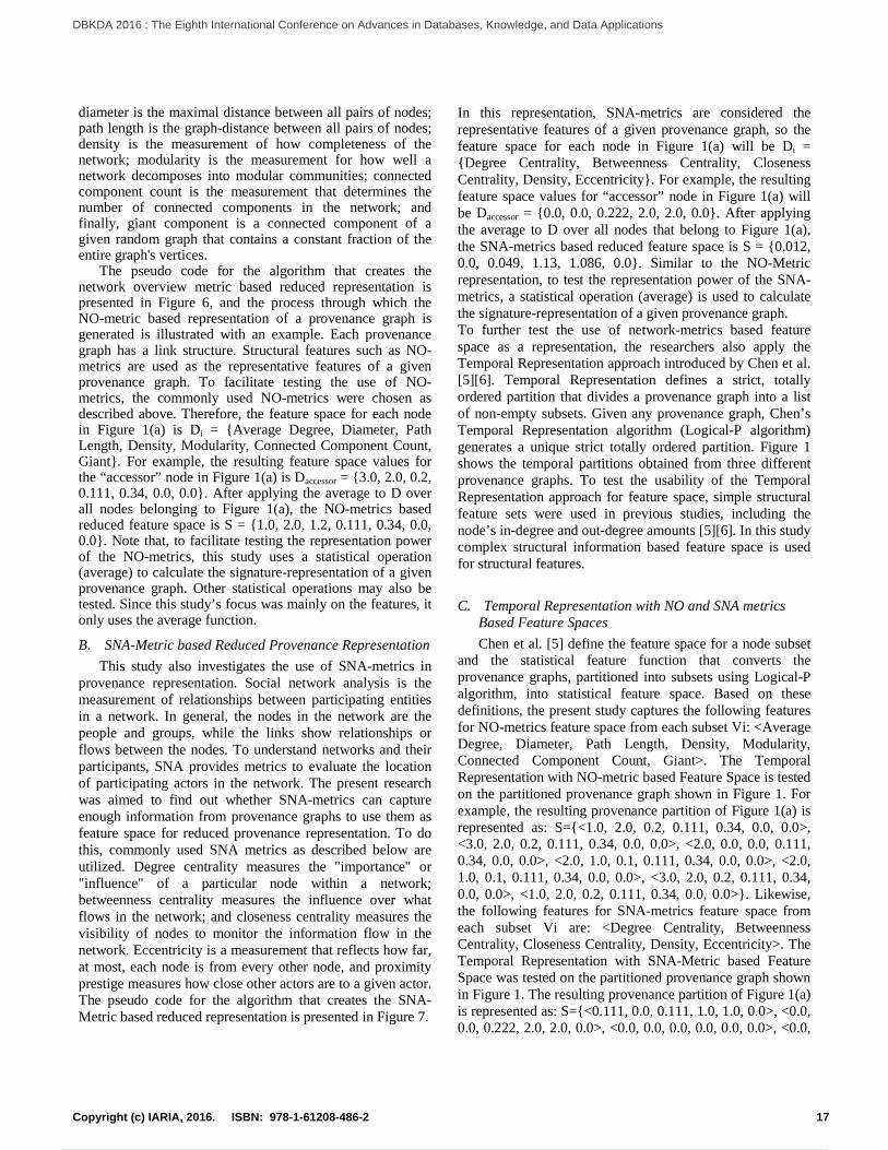
diameter is the maximal distance between all pairs of nodes;path length is the graph-distance between all pairs of nodes;density is the measurement of how completeness of thenetwork; modularity is the measurement for how well anetwork decomposes into modular communities; connectedcomponent count is the measurement that determines thenumber of connected components in the network; andfinally, giant component is a connected component of agiven random graph that contains a constant fraction of theentire graph's vertices.

The pseudo code for the algorithm that creates thenetwork overview metric based reduced representation ispresented in Figure 6, and the process through which theNO-metric based representation of a provenance graph isgenerated is illustrated with an example. Each provenancegraph has a link structure. Structural features such as NO-metrics are used as the representative features of a givenprovenance graph. To facilitate testing the use of NO-metrics, the commonly used NO-metrics were chosen asdescribed above. Therefore, the feature space for each nodein Figure 1(a) is Di = {Average Degree, Diameter, PathLength, Density, Modularity, Connected Component Count,Giant}. For example, the resulting feature space values forthe “accessor” node in Figure 1(a) is Daccessor = {3.0, 2.0, 0.2,0.111, 0.34, 0.0, 0.0}. After applying the average to D overall nodes belonging to Figure 1(a), the NO-metrics basedreduced feature space is S = {1.0, 2.0, 1.2, 0.111, 0.34, 0.0,0.0}. Note that, to facilitate testing the representation powerof the NO-metrics, this study uses a statistical operation(average) to calculate the signature-representation of a givenprovenance graph. Other statistical operations may also betested. Since this study’s focus was mainly on the features, itonly uses the average function.

B. SNA-Metric based Reduced Provenance Representation

This study also investigates the use of SNA-metrics inprovenance representation. Social network analysis is themeasurement of relationships between participating entitiesin a network. In general, the nodes in the network are thepeople and groups, while the links show relationships orflows between the nodes. To understand networks and theirparticipants, SNA provides metrics to evaluate the locationof participating actors in the network. The present researchwas aimed to find out whether SNA-metrics can captureenough information from provenance graphs to use them asfeature space for reduced provenance representation. To dothis, commonly used SNA metrics as described below areutilized. Degree centrality measures the "importance" or"influence" of a particular node within a network;betweenness centrality measures the influence over whatflows in the network; and closeness centrality measures thevisibility of nodes to monitor the information flow in thenetwork. Eccentricity is a measurement that reflects how far,at most, each node is from every other node, and proximityprestige measures how close other actors are to a given actor.The pseudo code for the algorithm that creates the SNA-Metric based reduced representation is presented in Figure 7.

In this representation, SNA-metrics are considered therepresentative features of a given provenance graph, so thefeature space for each node in Figure 1(a) will be Di ={Degree Centrality, Betweenness Centrality, ClosenessCentrality, Density, Eccentricity}. For example, the resultingfeature space values for “accessor” node in Figure 1(a) willbe Daccessor = {0.0, 0.0, 0.222, 2.0, 2.0, 0.0}. After applyingthe average to D over all nodes that belong to Figure 1(a),the SNA-metrics based reduced feature space is S = {0.012,0.0, 0.049, 1.13, 1.086, 0.0}. Similar to the NO-Metricrepresentation, to test the representation power of the SNA-metrics, a statistical operation (average) is used to calculatethe signature-representation of a given provenance graph.To further test the use of network-metrics based featurespace as a representation, the researchers also apply theTemporal Representation approach introduced by Chen et al.[5][6]. Temporal Representation defines a strict, totallyordered partition that divides a provenance graph into a listof non-empty subsets. Given any provenance graph, Chen’sTemporal Representation algorithm (Logical-P algorithm)generates a unique strict totally ordered partition. Figure 1shows the temporal partitions obtained from three differentprovenance graphs. To test the usability of the TemporalRepresentation approach for feature space, simple structuralfeature sets were used in previous studies, including thenode’s in-degree and out-degree amounts [5][6]. In this studycomplex structural information based feature space is usedfor structural features.

C. Temporal Representation with NO and SNA metricsBased Feature Spaces

Chen et al. [5] define the feature space for a node subsetand the statistical feature function that converts theprovenance graphs, partitioned into subsets using Logical-Palgorithm, into statistical feature space. Based on thesedefinitions, the present study captures the following featuresfor NO-metrics feature space from each subset Vi: <AverageDegree, Diameter, Path Length, Density, Modularity,Connected Component Count, Giant>. The TemporalRepresentation with NO-metric based Feature Space is testedon the partitioned provenance graph shown in Figure 1. Forexample, the resulting provenance partition of Figure 1(a) isrepresented as: S={<1.0, 2.0, 0.2, 0.111, 0.34, 0.0, 0.0>,<3.0, 2.0, 0.2, 0.111, 0.34, 0.0, 0.0>, <2.0, 0.0, 0.0, 0.111,0.34, 0.0, 0.0>, <2.0, 1.0, 0.1, 0.111, 0.34, 0.0, 0.0>, <2.0,1.0, 0.1, 0.111, 0.34, 0.0, 0.0>, <3.0, 2.0, 0.2, 0.111, 0.34,0.0, 0.0>, <1.0, 2.0, 0.2, 0.111, 0.34, 0.0, 0.0>}. Likewise,the following features for SNA-metrics feature space fromeach subset Vi are: <Degree Centrality, BetweennessCentrality, Closeness Centrality, Density, Eccentricity>. TheTemporal Representation with SNA-Metric based FeatureSpace was tested on the partitioned provenance graph shownin Figure 1. The resulting provenance partition of Figure 1(a)is represented as: S={<0.111, 0.0, 0.111, 1.0, 1.0, 0.0>, <0.0,0.0, 0.222, 2.0, 2.0, 0.0>, <0.0, 0.0, 0.0, 0.0, 0.0, 0.0>, <0.0,



28 / 107

0.0, 0.111, 1.0, 1.0, 0.0>, <0.0, 0.0, 0.111, 1.0, 1.0, 0.0>,<0.0, 0.0, 0.222, 2.0, 2.0, 0.0>, <0.111, 0.0, 0.111, 1.0, 1.0,0.0>}.

D. Feature Selection Methodology

The selection of an optimal feature set depends upon boththe mining targets and the nature of the provenance [5][6]. Inthis study, the target in unsupervised clustering is to grouptogether provenance instances based on their originalexperiment. Therefore, the aim is to select a feature set thatcan discriminate between provenance instances of differentexperiments. In other words, the distance between tworepresentations of provenance derived from the sameexperiment should be smaller than the distance betweenrepresentations of provenance derived from differentexperiments. More features result in more distinguishingpower while adding irrelevant features to a dataset oftendecreases the accuracy of the unsupervised clusteringapproaches. This study investigates whether networkoverview metrics or social network analysis metrics haveenough discriminating power for unsupervised clusteringtasks in scientific provenance datasets.

This study assumes that provenance graphs from relatedexperiments have similar structure and similar attributeinformation, while provenance graphs from differentexperiments are either different in attribute information or instructural information. To this end, while using any featureset, Figure 1(a) and Figure 1(b) should be clustered together.To test this assumption, the Euclidean distance, calculatedfrom the simple structural feature set (proposed by [5][6]),NO-metrics, and SNA-metrics based complex structuralfeature sets were investigated. The results of thisinvestigation are shown in Table I. These distances showwhether two graphs are relatively closer to each other fordiffering metrics. The results indicated that the distancebetween the provenance graphs in Figure 1(a) and Figure1(b) turned out to be closer to each other for certain featuresmore than others, meaning the distances calculated fromcomplex structural information based feature spacerepresentations had more distinguishing power compared toother representations. It is important to note that the valuesof features were normalized before calculating the EuclideanDistance to make sure that all metrics contribute equally tothe results. The normalized feature values scaled between 0and 1.

TABLE I. EUCLIDEAN DISTANCE FOR DIFFERING FEATURE SETSAMONGST DIFFERENT REPRESENTATIONS

Distance in Simple Structural Feature Set (from [5][6] )Figures1(a) – 1(b)

0.7454

Distance in NO-Metric Based Structural Feature SetFigures1(a) – 1(b)

0.5408

Distance in SNA-Metric Based Structural Feature SetFigures1(a) – 1(b)

0.4429

Chen reported that the disadvantage of the simplestructural feature set (i.e., amount of in-degree/out-degree) isthat if two provenance graphs have the same structure butdifferent node/edge information, it would be impossible todistinguish between the two through the structural feature setalone. To this end, Chen proposed an extension to the set byfurther splitting the edges into different types in OPM (i.e.,used, wasGeneratedBy, wasControlledBy, wasTriggeredBy,wasDerivedFrom), so that one can discriminate graphs thathave similar structure but are semantically different. Thepresent study follows similar methodology, but assignsdiffering weights to each semantically different edge. Indistinguishing the semantically different but structurally thesame provenance graphs, the approach works with bothnetwork overview and social network analysis metrics.

IV. METHODOLOGY

This study addresses whether it is possible to detectfailed workflows in a provenance dataset without theguidance of a workflow script or to detect provenancevariants caused by either workflow execution failure orprovenance capture failure. To answer these questions, theusability of complex structural information based reducedprovenance representations is explored with a focus onfinding variants to help detect faulty provenance data bychecking cluster centroids in the case where correct andfaulty provenances are naturally separated into differentclusters.

Much like the study by Chen et al., the present studyinvestigates the best unsupervised algorithm for the graphstructure based provenance representation from severalpopular clustering algorithms: centroid-based (k-means),distribution-based (DBScan), and density-based (EMalgorithm) [5][6]. Results indicated that the k-meansalgorithm produced the highest quality clusters. Hence, inthis study, the k-means algorithm was selected to show theusefulness of the proposed representations.

Weka libraries and SimpleKmeans were used in the k-means algorithm. Using Euclidean distance as the similarityfunction in k-means limited the application of k-means tosame-length representation. Since both NO-metric and SNA-metric based representations provide same-lengthrepresentation for all provenance graphs, this was notproblematic. However, when testing the temporalrepresentation with network-metric based representation, thisissue was limiting. To overcome this, the researchersfollowed the same approach as Chen et al., filling missingfeatures with a special value of 0 to provide goodperformance in clustering results.

V. EXPERIMENTAL EVALUATION

To prove that the provenance representations using thegraph partitioning approach can support scalable analysiswhile being resilient to errors in provenance data, theexperiment is conducted using a 10GB provenance databasewith known failure patterns [7]. This 10GB database ofprovenance is populated from a workload of roughly 48,000workflow instances that are modeled based on six real



29 / 107

workflows. The LEAD NAM, SCOOP, and NCSF areweather and ocean modeling workflows, Gene2Life andMOTIF are bioinformatics and biomedical workflows, andthe Animation workflow carries out computer animationrendering. Some of the workflows are small, having fewnodes and edges, while others like Motif have a few hundrednodes and edges. In the 10GB database, each of the sixworkflow types has 2000 instances per failure mode, withthe failure modes as following: No failures and droppednotifications (success case), 1% failure rate, 1% droppednotification rate, 1% failure rate, and 1% droppednotification rate.

The Karma provenance system is used to store the 10GBprovenance dataset and to export the provenance in the formof OPM graphs [9]. From the provenance graphs, theadjacency matrix is generated. Then the complex networkmetrics and social network analysis metrics are calculatedand stored.

The evaluation strategy used here follows themethodological analysis first described by Chen, Plale andAktas [5][6]. No structural information is assumed in therepresentation of the provenance datasets within the 10GBdatabase.

In order to help understand how the graph-structurebased representations identify clusters, NAM workflowprovenance datasets from weather forecast workflow werechosen, as Chen et al. identified that this is the bestillustration of provenance capture from scientific workflows[5][6]. The temporal representation of the NAM provenancedatasets has shown that NAM datasets include provenancegraphs with varying numbers of partitions, ranging from 2 to10. It turns out that a NAM provenance graph with 10subsets is a complete graph, while provenance graphs withless than 10 partitions are incomplete and caused by droppednotifications. To test the usefulness of the graph structurebased reduced representation approaches, a k-meansclustering algorithm was applied to the provenancerepresentations of NAM provenance datasets. Purity,Normalized Mutual Information (NMI), and Within-ClusterSum of Squares (WCSS) were used to compare theperformance of different clustering techniques.

The grouping of the NAM provenance dataset (based onthe temporal length defined by Chen et al.) is shown inFigure 2. The grouping results indicate that 78% of the NAMprovenance graphs have the largest possible number ofpartitions, and 6% of the graphs have small partitionsranging from 2 to 4. Small-partitioned provenance graphsindicate dropped notifications or early failures that mighthappen in the NAM workflow execution.

Figure 2. NAM workflow clusters - Grouping Based on TemporalRepresentation

To test the clustering on the reduced representations, thegrouping results (shown in Figure 2) are used as the goldenstandard for Purity and NMI metrics. The clustering isevaluated on both NO-metric and SNA-metric based reducedprovenance representations. The SimpleKMeans clusteringalgorithm with Euclidean Distance measurement is thenapplied to these representations. Unlike the temporalrepresentation, the graph structure based representation hasrepresentation sequences of uniform length. Thus, the k-means clustering algorithm is applied without anylimitations.

TABLE II. NAM WORKFLOW CLUSTERING RESULTS FOR K=9AND VARYING REDUCED PROVENANCE REPRESENTATIONS

Purity NMI WCCSNetwork

Overview 0.798375 0.503209 171.6229SNA 0.922 0.516648 43.1794

TR+SNA 0.938625 0.555053 561.3776

Table II gives the summary of the quality of clusteringresults when k = 9. The results indicate that SNA-metricbased representation and Temporal Partitioning with SNArepresentation lead to high quality clustering results. SNAmetrics were better than NO metrics in capturing thecomplex structural information as features. Purity and NMImetrics were computed by calculating the correctly assignedworkflow instances. To do this, the grouping results shownin Figure 2 were used as the golden standard. To furtherunderstand the behavior of clustering for varying reducedrepresentation sizes, different k values were tested. Tochoose the number of cluster k, the quality of resultingclusters was plotted by computing Purity as an externalevaluation criterion.

0

0,5

1

1,5

2 3 4 5 6 7 8 9

NetworkOverview

TR+SNA

SNA

Figure 3. NAM - Purity results



30 / 107

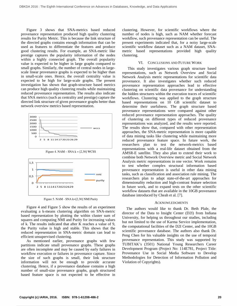
Figure 3 shows that SNA-metrics based reducedprovenance representation produced high quality clusteringresults for Purity Metric. This is because the link structure ofthe directed graphs contains enough information that can beused as features to differentiate the features and producegood clustering results. For example, an SNA-metric likeprestige captures the popularity information of the nodeswithin a highly connected graph. The overall popularityvalue is expected to be higher in large graphs compared tosmall graphs. Similarly, the number of central nodes in large-scale linear provenance graphs is expected to be higher thanin small-scale ones. Hence, the overall centrality value isexpected to be high for large-scale graphs. The presentinvestigation has shown that graph-structure based metricscan produce high quality clustering results while maintainingreduced provenance representation. The results also indicatethat SNA metrics (such as centrality and prestige) capture thedirected link structure of given provenance graphs better thannetwork overview metrics based representation.

0

500

1000

1500

2000

2500

3000

2 5 8 11 14 17 20 23 26 29

wccs

Figure 4. NAM – SNA k = [2,30] WCSS

0

0,5

1

1,5

2 5 8 11141720232629

nmi

purity

Figure 5. NAM - SNA k=[2,30] NMI Purity

Figure 4 and Figure 5 show the results of an experimentevaluating a k-means clustering algorithm on SNA-metricbased representation by plotting the within cluster sum ofsquares and computing NMI and Purity for increasing valuesof k. The results indicated that after K reaches a value of 9,the Purity value is high and stable. This shows that thereduced representation in SNA-metric domain can lead toefficient unsupervised clustering.

As mentioned earlier, provenance graphs with fewpartitions indicate small provenance graphs. These graphsare often incomplete and may be caused by early failures inworkflow execution or failures in provenance capture. Sincethe size of such graphs is small, their link structureinformation will not be enough to provide accurateclustering. Hence, if a provenance database contains a highnumber of small-size provenance graphs, graph structuredbased feature space is not expected to be effective in

clustering. However, for scientific workflows where thenumber of nodes is high, such as NAM whether forecastworkflow, such provenance representation can be useful. Thepresent experiments indicated that, for a noisy large-scalescientific workflow dataset such as a NAM dataset, SNA-metric based representations provided high qualityclustering.

VI. CONCLUSIONS AND FUTURE WORK

This study investigates various graph structure basedrepresentations, such as Network Overview and SocialNetwork Analysis metric representations for scientific dataprovenance. It also investigates whether such reducedprovenance representation approaches lead to effectiveclustering on scientific data provenance for understandingthe hidden structures within the execution traces of scientificworkflows. Clustering was applied to the graph structurebased representations on 10 GB scientific dataset todetermine their usefulness. The graph structure basedprovenance representations were compared against otherreduced provenance representation approaches. The qualityof clustering on different types of reduced provenancerepresentations was analyzed, and the results were reported.The results show that, compared with other representationapproaches, the SNA-metric representation is more capableof data mining tasks like clustering while maintaining morereduced provenance feature space. In future work, theresearchers plan to test the network-metrics basedrepresentations with a real-life dataset obtained from theAMSR-E satellite. They also plan to extend their work tocombine both Network Overview metric and Social NetworkAnalysis metric representations in one vector. Work remainsto test whether complex structural information basedprovenance representation is useful in other data miningtasks, such as classification and association rule mining. Theresearchers plan to adapt state-of-the-art approaches fordimensionality reduction and high-contrast feature selectionin future work, and to expand tests on the other scientificworkflow datasets that are available in the 10GB provenancedatabase introduced by Cheah et al. [7].

ACKNOWLEDGMENTS

The authors would like to thank Dr. Beth Plale, thedirector of the Data to Insight Center (D2I) from IndianaUniversity, for helping us throughout our studies, includingbut not limited to the use of Karma Service implementation,the computational facilities of the D2I Center, and the 10GBscientific provenance database. The authors also thank Dr.Peng Chen for his valuable insights on the use of temporalprovenance representation. This study was supported byTUBITAK’s (3501) National Young Researchers CareerDevelopment Program (Project No: 114E781, Project Title:Provenance Use in Social Media Software to DevelopMethodologies for Detection of Information Pollution andViolation of Copyrights).



31 / 107

REFERENCES

[1] C. M. Antunes, and A. L. Oliveira, “Temporal data mining: Anoverview” KDD Workshop on Temporal Data Mining, 2001, pp. 1–13.

[2] M. Aktas, B. Plale, D. Leake and N. K. Mukhi, “UnmanagedWorkflows: Their Provenance and Use”, Q. Bai, Q. Liu eds. DataProvenance and Data Management in eScience, Studies inComputational Intelligence series, Springer, Vol 426, 2013, pp. 59-81.

[3] S. Bechhofer, D. D. Roure, M. Gamble, C. Goble and L. Buchan,“Research objects: Towards exchange and reuse of digitalknowledge” The Future of the Web for Collaborative Science, 2010.

[4] L. Moreau, and et al., “The open provenance model corespecification (v1. 1)” Future Generation Computer Systems. 27, 2011,pp. 743–756.

[5] P. Chen, and B. Plale, and M. Aktas, “Temporal representation forscientific data provenance” eScience 2012, pp. 1-8.

[6] P. Chen, and B. Plale, and M. Aktas, “Temporal Representation forMining Scientific Data Provenance” Future Generation Comp. Syst.36, 2014, pp. 363-378.

[7] Y. Cheah, B. Plale, J. Kendall-Morwick, D. Leake and L.Ramakrishnan, “A Noisy 10GB Provenance Database” 2nd Int’lWorkshop on Traceability and Compliance of Semi-StructuredProcesses (TC4SP), co-located with Business Process Management(BPM), 2011, pp. 370-381.

[8] R. Agrawal and R. Srikant, “Fast algorithms for mining associationrules” 20th Int. Conf. Very Large Data Bases, VLDB. 1215, pp. 487-499, 1994.

[9] Y. L. Simmhan, B. Plale, and D. Gannon, “A Survey of DataProvenance in e-Science” ACM SIGMOD Record. 34, 2005, pp. 31–36.

[10] S. B. Davidson and J. Freire, “Provenance and scientific workflows:challenges and opportunities” SIGMOD Conf., 2008, pp. 1345–1350.

[11] E. Santos, L. Lins, J. P. Ahrens, J. Freire, and C. T. Silva, “A firststudy on clustering collections of workflow graphs” IPAW, 2008, pp.160-173.

[12] R. Bose and J. Frew., “Lineage retrieval for scientific data processing:a survey” ACM Comput. Surv. 37(1), March 2005, pp. 1-28.



32 / 107

Figure 6. Pseudo code for the algorithm CN metrics based reduced provenance representation

Figure 7. Pseudo code for the algorithm SNA metrics based reduced provenance representation

1: assign 0 to total_avg, total_dia, total_pLen, total_dns, total_mdl, total_ccc, total_gia2: for all nodes n in D do3: assign convertOPMtoAdjacencyMatrix(n) to adjacency_matrix4: assign averageDegree(adjacency _matrix) to avg5: assign diameter(adjacency _matrix) to dia6: assign pathLength(adjacency _matrix) to pLen7: assign density(adjacency_matrix) to dns8: assign modulartiy(adjacency_matrix) to mdl9: assign connectedComponentCount(adjacency_matrix) to ccc10: assign giant (adjacency_matrix) to gia11: assign total_avg + avg to total_avg; total_dia + dia to total_dia; total_pLen + pLen to total_pLen;total_dns + dns to total_dns; total_mdl + mdl to total_mdl; total_ccc + ccc to total_ccc; total_gia + gia to total_gia12: end for13: assign {total_avg/n, total_dia/n, total_pLen/n, total_dns/n, total_mdl/n, total_ccc/n, total_gia/n} to Feature_Space

1:T <- set of all node in G2:for all node k in T do3: assign empty to Stack(S)4: assign empty to LinkedList(Q)5: addLast k to LinkedListQ)6: while LinkedList(Q) is not empty do7: assign removeFirst from LinkedList(Q) to v8: add Stack(S) to v9: for all edge of v do10: add opposite node to Linked(Q)11: end for12: end while13: for all nodes in T do14: if count of neighbour of s > 0 do15: add count of neighbour of s to closenessCentrality16: add count of neighbour of s to proximityPrestige17: add max in count of neighbour of s or eccentricity of s to eccenricity18: end if19: end for20: for all out going edges from s do21: if count of neighbour of s > 0 do22: add count of neighbour of s to degreeCenrality23: end if24: end for25: for all incoming edges from s do26: if count of neighbour of s > 0 do27: add count of neighbour of s to degreePrestige28: end if29: end for30: if s is reachable from other nodes31: closenessCentrality /= reachableCount32: proximityPrestige /= reachableCount33: end if34: closenessCentrality /= All nodes count - 135: degreeCentrality /= All nodes count - 136: degreePrestige /= All nodes count - 137:end for38:do normalization for all attributes of SNA



33 / 107

An Efficient Algorithm for Read Matching in DNA Databases

Yangjun Chen, Yujia Wu

Dept. Applied Computer Science

University of Winnipeg, Canada

email: [email protected], [email protected]

Jiuyong Xie

Dept. Physiology &Pathophysiology, College of Medicine

University of Manitoba, Canada

email: [email protected]

Abstract—In this paper, we discuss an efficient and effective

index mechanism to support the matching of massive reads

(short DNA strings) in DNA databases. It is very important to the

next generation sequencing in the biological research. The main

idea behind it is to construct a trie structure over all the reads,

and search the trie against a BWT-array L created for a genome

sequence s to locate all the occurrences of every read in s once for

all. In addition, we change a single-character checking against L

to a multiple-character checking, by which multiple searches of L

are reduced to a single scanning of L. In this way, high efficiency

can be achieved. Experiments have been conducted, which show

that our method for this problem is promising.

Keywords—string matching; DNA sequences; tries; BWT-

transformation

I. INTRODUCTION

The recent development of next-generation sequencing has changed the way we carry out the molecular biology and genomic studies. It has allowed us to sequence a DNA (Deoxyribonucleic acid) sequence at a significantly increased base coverage, as well as at a much faster rate. This facilitates building an excellent platform for the whole genome sequencing, and for a variety of sequencing-based analysis, including gene expressions, mapping DNA-protein interactions, whole-transcriptome sequencing, and RNA (Ribonucleic acid) splicing profiles. For example, the RNA-Seq protocol, in which processed mRNA is converted to cDNA and sequenced, is enabling the identification of previously unknown genes and alternative splice variants. The whole-genome sequencing of tumour cells can uncover previously unidentified cancer-initiating mutations.

The core and the first step to take advantage of the new sequencing technology is termed as read aligning, where a read is a short nucleotide sequence of 30 - 1000 base pairs (bp) generated by a high throughput sequencing machine made by Illumina, Roche, ABI/Life Technologies, which is in fact a sequence fragment fetched from a longer DNA molecule present in a sample that is fed into the machine. Most of the next-generation sequencing projects begin with a reference sequence which is a previously well studied, known genome. The process of a read aligning is to find the meaning of reads, or in other words, to determine their positions within a reference sequence, which will then be used for an effective statistical analysis.

Compared to the traditional pattern matching problems, the new challenge from the read aligning is its enormous volume, usually millions to billions of reads need to be aligned within

a same reference sequence. For example, to sequence a human molecule sample with 15X coverage, one may need to align 1.5 billion reads of length about 100 characters (bps).

In general, three kinds of alignment algorithms are practically applied: hash-based, string-matching-based, as well as inexact matching (including edit-distance computation and k-mismatching). By the hash-based methods, short subsequences called seeds are extracted from a pattern sequence and their hash values are computed, which are used to search against a reference genome sequence. By the string-matching-based methods, different efficient algorithms are utilized, such as Knuth-Morris-Pratt [22], Boyer-Moore [9], and Apostolico-Giancarlo [3], as well as the algorithms based on different indexes like suffix trees [37][45], suffix arrays [35], and BWT-transformation (Burrows-Wheeler Transform) [10, 16, 40]. By the edit-distance computation, a score matrix to represent the relevance between characters is defined and an alignment with the highest total score is searched, for which the dynamical programming paradigm is typically employed. However, a recent research shows that the BWT can also be used as an index structure for the k-mismatching problem [30].

All the methods mentioned above are single-pattern oriented, by which a single string pattern is checked against an entire database to find all the alignments in all the sequences stored in the database. In the current research of the molecular biology, however, we need to check a bunch of string patterns each time and the size of all string patterns can be even much larger than the database itself. This requires us considering all the string patterns as a whole, rather than separately check them one by one. By the Aho-Corasick algorithm [1], the multiple patterns are handled. However, it cannot be utilized in an indexing environment since it has to search a target sequence linearly while by using indexes to expedite a search this is not expected.

In this paper, we address this issue and present a holistic string matching algorithm to handle million-billion reads. Our experiment shows that it can be more than 40% faster than single-pattern oriented methods when multi-million reads are checked. The main idea behind our method is: 1. Construct a trie T over all the pattern sequences, and check

T against a BWT-array created as an index for a target (reference) sequence. This enables us to avoid repeated search of the same part of different reads.

2. Change a single-character checking to a multiple-character checking. (That is, each time a set of characters respectively from more than one read will be checked



34 / 107

against a BWT-array in one scan, instead of checking them separately one by one in multiple scans.) In this way, high efficiency has been achieved. The remainder of the paper is organized as follows. In

Section II, we review the related work. In Section III, we briefly describe a string matching algorithm based on the BWT-transformation. In Section IV, we discuss our basic algorithm in great detail. In Section V, we improve the basic method by using multiple-character checkings. Section VI is devoted to the test results. Finally, a short conclusion is set forth in Section VII.

II. RELATED WORK

The matching of DNA sequences is just a special case of the general string matching problem, which has always been one of the main focuses in the computer science. All the methods developed up to now can be roughly divided into two categories: exact matching and inexact matching. By the former, all the occurrences of a pattern string p in a target string s will be searched. By the latter, a best alignment between p and s (i.e., a correspondence with the highest score) is searched in terms of a given score matrix M, which is established to indicate the relevance between characters (more exactly, the meanings represented by them).

A. Exact Matching

Scanning-based By this kind of algorithms, both pattern p and s are scanned from left to right, but often with an auxiliary data structure used to speed up the search, which is typically constructed by a pre-processor. The first of them is the famous Knuth-Morris-Pratt algorithm [22], which employs an auxiliary next-table (for p) containing the so-called shift information (or say, failure function values) to indicate how far to shift the pattern from right to left when the current character in p fails to match the current character in s. Its time complexity is bounded by O(m + n), where m = |p| and n = |s|. The Boyer-Moore approach [9] works a little bit better than the Knuth-Morris-Pratt. In addition to the next-table, a skip-table (also for p) is kept. For a large alphabet and small pattern, the expected number of character comparisons is about n/m, and is O(m + n) in the worst case. Although these two algorithms have never been used in practice, they sparked a series of research on this problem, and improved by different researchers in different ways, such as the algorithms discussed in [1][27]. However, the worst-case time complexity remains unchanged. The idea of the ‘shift information’ has also been adopted by Aho and Corasick [1] for the multiple-string matching, by which s is searched for an occurrence of any one of a set of k patterns: {p1, p2, …, pk}. Their algorithm needs

only O(

k

iim

1

+ n) time, where mi = |pi| (i = 1, …, k). However,

this algorithm cannot be adapted to an index environment due its working fashion totally unsuitable for indexes.

Index-based In situations where a fixed string s is to be searched repeatedly, it is worthwhile constructing an index over s [46], such as suffix trees [37][45], suffix arrays [35], and more recently the BWT-transformation [10][16][30][31][40]. A suffix tree is in fact a trie structure [21] over all the suffixes of s; and by using the Weiner’s

algorithm it can be built in O(n) time [37]. However, in comparison with suffix trees, the BWT-transformation is more

suitable for DNA sequences due to its small alphabet since

the smaller is, the smaller space will be occupied by the corresponding BWT index. According to a survey done by Li and Homer [30] on sequence alignment algorithms for next-generation sequencing, the average space required for each character is 12 - 17 bytes for suffix trees while only 0.5 - 2 byte for the BWT. Our experiments also confirm this distinction. For example, the file size of chromosome 1 of human is 270 Mb. But its suffix tree is of 26 Gb in size while its BWT needs only 390 Mb – 1 Gb for different compression rates of auxiliary arrays, completely handlable on PC or laptop machines. The huge size of a suffix tree may greatly affect the computation time. For example, for the Zebra fish and Rat genomes (sizes 1,464,443,456 pb, and 2,909,701,677 pb, respectively), we cannot finish the construction of their suffix trees within two days in a computer with 32GB RAM.

Hash-based Intrinsically, all hash-table-based algorithms [18, 20] extract short subsequences called 'seeds' from a pattern sequence p and create a signature (a bit string) for each of them. The search of a target sequence s is similar to that of the Brute Force searching, but rather than directly comparing the pattern at successive positions in s, their respective signatures are compared. Then stick each matching seed together to form a complete alignment. Its expected time is O(m + n), but in the

worst case, which is extremely unlikely, it takes O(mn) time. The hash technique has also been extensively used in the DNA sequence research [19, 28, 29, 34, 39], and all experiments shows that they are generally inferior to the suffix tree and the BWT index in both running time and space requirements.

B. Inexact Matching

The inexact matching ranges from the score-based to the k-mismatching, as well as the k-error. By the score-based

method, a score matrix M of size || || is used to indicate the relevance between characters. The algorithm designed is to find the best alignment (or say, the alignment with the highest scores) between two given strings, which can be DNA sequences, protein sequences, or XML documents; and the dynamic programming paradigm is often utilized to solve the problem [14]. By the k-mismatching, we will find all those

subsequences q of s such that d(p, q) k, where d( ) is a distance function. When it is the Hemming distance, the problem is known as sequence matching with k mismatches [4]. When it is the Levenshtein distance, the problem is known as sequence matching with k errors [6]. There is a bunch of algorithms proposed for this problem, such as [4, 5, 24, 25, 42, 43] for the k-mismatch; and [6, 11, 15, 44] for the k-error. All

the methods for the k-mismatch needs quadratic time O(mn) in the worst case. However, the algorithm discussed in [2] has

the best expected time complexity O(n k logm). Especially,

for small k and large , the search requires sublinear time on average. In addition, the BWT can also be used as an index structure for this problem [30]. For the k-error, the worst case time complexity is the same as the k-mismatching. But the

expected time can reach O(kn) by an algorithm discussed in [11]. As a different kind of inexact matching, the string matching with Don’t-Cares (or wild-cards) has also been an



35 / 107

active research topic for decades, by which we may have wild-cards in p, in s, or in both of them. A wild card matches any character. Due to this property, the ‘match’ relation is no longer transitive, which precludes straightforward adaption of the shift information used by Knuth-Morris-Pratt and Boyer-Moore. All the methods proposed to solve this problem also needs quadratic time [38]. But using a suffix array as the index, however, the searching time can be reduced to O(logn) for some patterns, which contain only a sequence of consecutive Don’t Cares [36].

III. BWT-TRANSFORMATION

In this section, we give a brief description of the BWT transformation to provide a discussion background.

A. BWT and String Compression

We use s to denote a string that we would like to transform. Assume that s terminates with a special character $, which does not appear elsewhere in s and is alphabetically prior to all other characters. In the case of DNA sequences, we have $ < A < C < G < T. As an example, consider s = acagaca$. We can rotate s consecutively to create eight different strings as shown in Figure 1(a).

By writing all these strings stacked vertically, we generate

an n n matrix, where n = |s| (see Figure 1(a).) Here, special

attention should be paid to the first column, denoted as F, and

the last column, denoted as L. For them, the following

equation, called the LF mapping, can be immediately observed:

F[i] = L[i]’s successor, (1)

where F[i] (L[i]) is the ith

element of F (resp. L).

From this property, another property, the so-called rank

correspondence can be derived, by which we mean that for

each character, its ith appearance in F corresponds to its ith

appearance in L, as demonstrated in Figure 1(b), in which the

position of a character (in s) is represented by its subscript.

(That is, we rewrite s as a1c1a2g1a3c2a4$.) For example, a2

(representing the 2nd appearance of a in s) is in the second

place among all the a-characters in both F and L while c1 the

first apperance in both F and L among all the c-characters. In

the same way, we can check all the other appearances of

different characters.

Now we sort the rows of the matrix alphabetically. We

will get another matrix, called the Burrow-Wheeler Matrix [7]

[12][23] and denoted as BWM(s), as demonstrated in Figure

1(c). Especially, the last column of BWM(s), read from top to

bottom, is called the BWT-transformation (or the BWT-array)

and denoted as BWT(s). So for s = acagaca$, we have BWT(s)

= acg$caaa.

By the BWM matrix, the LF-mapping is obviously not

changed. Surprisingly, the rank correspondence also remains.

Even though the ranks of different appearances of a certain

character (in F or in L) may be different from before, their

rank correspondences are not changed as shown in Figure 2(b),

in which a2 now appears in both F and L as the fourth element

among all the a-characters, and c1 the second element among

all the c-characters.

The first purpose of BWT(s) is for the string compression

since same characters with similar right-contexts in s tend to

be clustered together in BWT(s), as shown by the following

example [10][16][40]:

BWT(tomorrow and tomorrow and tomorrow)

= wwwdd nnoooaatttmmmrrrrrrooo $ooo

Such a transformed string can be effectively compressed and then decompressed. Due to the LF-mapping and the rank correspondence, it can also be easily restored to the original string.

The second purpose is for the string search, which will be discussed in the next subsection in great detail. We need this part of knowledge to develop our method.

B. String Search Using BWT

For the purpose of the string search, the character

clustering in F has to be used. Especially, for any DNA

sequence, the whole F can be divided into five or less

segments: $-segment, A-segment, C-segment, G-segment, and

T-segment, denoted as F$, FA, FC, FG, FT, respectively. In

addition, for each segment in F, we will rank all its elements

from top to bottom, as illustrated in Figure 2(a). $ is not

ranked since it appears only once.

From Figure 2(a), we can see that the rank of a4, denoted

as rkF(a4), is 1 since it is the first element in FA. For the same

reason, we have rkF(a3) = 2, rkF(a1) = 3, rkF(a2) = 4, rkF(c2) =

1, rkF(c1) = 2, and rkF(g1) = 1.

It can also be seen that each segment in F can be

effectively represented as a triplet of the form: <; x, y>,

where {$}, and x, y are the positions of the first

and last appearance of in F, respectively. So the whole F

Figure 2. LF-mapping and tank-correspondence

$ a4

a4 c2

c2 a3

a3 g1

g1 a2

a2 c1

c1 a1

a1 $

F L

(a) (b)

1

1

2

1

4

2

3

rkF

1

2

1

4

2

3

By ranking the

elements in F, each element in

L is also ranked

with the same number.

rkL

F$ = <$; 1, 1>

Fa = <a; 2, 5>

Fc = <c; 6, 7>

Fg = <g; 8, 8>

Figure 1. Rotation of a string

$ a c a g a c a

a c a g a c a $ c a g a c a $ a a g a c a $ a c

g a c a $ a c a a c a $ a c a g c a $ a c a g a a $ a c a g a c

$ a c a g a c a a $ a c a g a c

c a $ a c a g a

a c a $ a c a g

g a c a $ a c a

a g a c a $ a c

c a g a c a $ a

a c a g a c a $

(a) (c)

a

g

a

c

a

$

(b)

a

g

a

c

a

$

a1 $

c1 a1

c2 a3

a2 c1

$ a4

a3 g1

a4 c2

g1 a2

F L

F L



36 / 107

can be effectively compacted and represented as a set of || +

1 triplets, as illustrated in Figure 2(b).

Now, we consider j (the jth appearance of in s).

Assume that rkF(j) = i. Then, the position where j appears in

F can be easily determined:

F[x + i - 1] = j. (2)

Besides, if we rank all the elements in L top-down in such a

way that an j is assigned i if it is the ith appearance among all

the appearances of in L. Then, we will have

rkF(j) = rkL(j), (3)

where rkL(j) is the rank assigned to j in L.

This equation is due to the rank correspondence between F

and L. (See [10][16][40] for a detailed discussion. Also see

Figure 2(a) for ease of understanding.)

With the ranks established, a string matching can be very

efficiently conducted by using the formulas (2) and (3). To see

this, let’s consider a pattern string p = aca and try to find all

its occurrences in s = acagaca$.

We work on the characters in p in the reverse order.

First, we check p[3] = a in the pattern string p, and then

figure out a segment in L, denoted as L, corresponding to Fa =

<a; 2, 5>. So L = L[2 .. 5], as illustrated in Figure 3(a), where

we still use the non-compact F for explanation. In the second

step, we check p[2] = c, and then search within L to find the

first and last c in L. We will find rkL(c2) = 1 and rkL(c1) = 2.

By using (3), we will get rkF(c2) = 1 and rkF(c1) = 2. Then, by

using (2), we will figure out a sub-segment F in F: F[xc + 1 -

1 .. xc + 2 - 1] = F[6 + 1 - 1 .. 6 + 2 - 1] = F[6 .. 7]. (Note that

xc = 6. See Figure 2(b) and Figure 3(b).) In the third step, we

check p[1] = a, and find L = L[6 .. 7] corresponding to F =

F[6 .. 7]. Repeating the above operation, we will find rkL(a3) =

2 and rkL(a1) = 3. See Figure 3(c). Since now we have

exhausted all the characters in p and F[xa + 2 – 1, xa + 3 – 1] =

F[3, 4] contains only two elements, two occurrences of p in s

are found. They are a1 and a3 in s, respectively.

C. RankAll

The dominant cost of the above process is the searching of L in each step. However, this can be dramatically reduced by

arranging || arrays each for a character such that [i]

(the ith entry in the array for ) is the number of appearances

of within L[1 .. i]. See Figure 4(a) for illustration.

Now, instead of scanning a certain segment L[x .. y] (x y)

to find a subrange for a certain , we can simply look up

the array for to see whether [x - 1] = [y]. If it is the case,

then does not occur in L[x .. y]. Otherwise, [[x - 1] + 1,

[y]] should be the found range. For example, to find the first

and the last appearance of c in L[2 .. 5], we only need to find

c[2 – 1] = c[1] = 0 and c[5] = 2. So the corresponding range is

[c[2 - 1] + 1, c[5]] = [1, 2].

In this way, the searching of L can be saved and we need

only a constant time to determine a subrange for a character

encountered during a pattern searching.

The problem of this method is its high space requirement,

which can be mitigated by replacing [] with a compact array

A for each , in which, rather than for each L[i] (i

{1, …, n}), only for some entries in L the number of their

appearances will be stored. For example, we can divide L into

a set of buckets of the same size and only for each bucket a

value will be stored in A. Obviously, doing so, more search

will be required. In practice, the size of a bucket (referred to

as a compact factor) can be set to different values. For

example, we can set = 4, indicating that for each four

contiguous elements in L a group of || integers (each in an A)

will be stored. That is, we will not store all the values in

Figure 4(a), but only store $[4], a[4], c[4], g[4], t[4], and $[8],

a[8], c[8], g[8], t[8] in the corresponding compact arrays, as

shown in Figure 4(b). However, each [j] for can be

easily derived from A by using the following formulas:

[j] = A[i] + , (4)

where i = j/ and is the number of ’s appearances within

L[i + 1 .. j], and

[j] = A[i] - , (5)

where i = j/ and is the number of ’s appearances within

L[j + 1 .. i].

Thus, we need two procedures: sDown(L, j, , ) and

sUp(L, j, , ) to find and , respectively. In terms of

whether j - i i - j, we will call sDown(L, j, , ) or

sUp(L, j, , ) so that fewer entries in L will be scanned to

find [j]. Finally, we notice that the column for $ can always be

divided into two parts. In the first part, each entry is 0 while in the second part each entry is 1 (see Figure 4(a)). So we can

Figure 3. Sample trace

$ a4 1

a4 c2 1

c2 a3 2

a3 g1 1

g1 a2 4

a2 c1 2

c1 a1 3

a1 $

F L

(a) (b)

$ a4 1

a4 c2 1

c2 a3 2

a3 g1 1

g1 a2 4

a2 c1 2

c1 a1 3

a1 $

F L

$ a4 1

a4 c2 1

c2 a3 2

a3 g1 1

g1 a2 4

a2 c1 2

c1 a1 3

a1 $

F L

To find

the first c

to find

the last c to find

the first a

to find

the last a

(c)

rkL

rkL

rkL

Figure 4. LF-mapping and rank-correspondence

$ a4

a4 c2

c2 a3

a3 g1

g1 a2

a2 c1

c1 a1

a1 $

F L

0

1

0

1

1

1

$

1

1

2

1

4

1

3

1

a

0

1

2

1

2

2

2

1

c

0

0

1

1

1

1

1

1

g

0

0

0

0

0

0

0

0

t

4

1

Aa

2

1

Ac

1

1

Ag

0

0

At

0 0 0 0

i

2

1

0

2

6

3

8

5

7

j

(a) (b)

For each = 4 values in L, a rankAll value is stored.



37 / 107

simply keep a number to indicate where it is divided, instead of storing the whole column.

D. Construction of BWT arrays

For self-explanation, we describe how a BWT array is constructed [10][16][26][40] in this subsection.

As mentioned above, a string s = a0a1 ... an−1 is always

ended with $ (i.e., ai for i = 0, …, n – 2, and an−1 = $). Let s[i] = ai (i = 0,1, …, n – 1) be the ith character of s, s[i.. j] = ai ... aj a substring and s[i .. n − 1] a suffix of s. Suffix array H of s is a permutation of the integers 0, ..., n − 1 such that H[i] is the start position of the ith smallest suffix. The relationship between H and the BWT array L can be determined by the following formulas:

Once L is determined. F can also be created immediately

by using formula (1).

IV. MAIN ALGORITHM

In this section, we present our algorithm to search a bunch

of reads against a genome s. Its main idea is to organize all the

reads into a trie T and search T against L to avoid any possible

redundancy. First, we present the concept of tries in

Subsection A. Then, in Subsection B, we discuss our basic

algorithm for the task. We improve this algorithm in Section

V.

A. Tries over Reads

Let D = {s1, …, sn} be a DNA database, where each si (i =

1, …, n) is a genome, a very long string *

( = {A, T, C,

G}). Let R = {r1, …, rm} be a set of reads with each rj being a

short string *. The problem is to find, for every rj’s (j =

1, …, m), all their occurrences in an si (i = 1, …, n) in D.

A simple way to do this is to check each rj against si one by

one, for which different string searching methods can be used,

such as suffix trees [37][45], BW-transformation [10], and so

on. Each of them needs only a linear time (in the size of si) to

find all occurrences of rj in si. However, in the case of very

large m, which is typical in the new genomic research, one-by-

one search of reads against an si is no more acceptable in

practice and some efforts should be spent on reducing the

running time caused by huge m.

Our general idea is to organize all rj’s into a trie structure

T and search T against si with the BW-transformation being

used to check the string matching. For this purpose, we will

first attach $ to the end of each si (i = 1, …, n) and construct

BWT(si). Then, attach $ to the end of each rj (j = 1, …, m) to

construct T = trie(R) over R as below.

If |R| = 0, trie(R) is, of course, empty. For |R| = 1, trie(R)

is a single node. If |R| > 1, R is split into || = 5 (possibly

empty) subsets R1, R2, …, R5 so that each Ri (i {1, …, 5})

contains all those sequences with the same first character i

{A, T, C, G} {$}. The tries: trie(R1), trie(R2), …, trie(R5)

are constructed in the same way except that at the kth step, the

splitting of sets is based on the kth characters in the sequences.

They are then connected from their respective roots to a single

node to create trie(R).

Example 1 As an example, consider a set of four reads:

r1: ACAGA

r2: AG

r3: ACAGC

r4: CA

For these reads, a trie can be constructed as shown in Figure

5(a). In this trie, v0 is a virtual root, labeled with an empty

character while any other node v is labeled with a real

character, denoted as l(v). Therefore, all the characters on a

path from the root to a leaf spell a read. For instance, the path

from v0 to v8 corresponds to the third read r3 = ACAGC$. Note

that each leaf node v is labelled with $ and associated with a

read identifier, denoted as (v).

C

The size of a trie can be significantly reduced by replacing

each branchless path segment with a single edge. By a

branchless path we mean a path P such that each node on P,

except the starting and ending nodes, has only one incoming

and one outgoing edge. For example, the trie shown in Figure

5(a) can be compacted to a reduced one as shown in Figure

5(b).

B. Integrating BWT Search with Trie Search

It is easy to see that exploring a path in a trie T over a set

of reads R corresponds to scanning a read r R. If we explore,

at the same time, the L array established over a reversed

genome sequence s , we will find all the occurrences of r

(without $ involved) in s. This idea leads to the following

algorithm, which is in essence a depth-first search of T by

using a stack S to control the process. However, each entry in

S is a triplet <v, a, b> with v being a node in T and a b, used

to indicate a subsegment in Fl(v)[a .. b]. For example, when

searching the trie shown in Figure 5(a) against the L array

shown in Figure 2(a), we may have an entry like <v1, 1, 4> in

S to represent a subsegment FA[1 .. 4] (the first to the fourth

entry in FA) since l(v1) = A. In addition, for technical

convenience, we use F to represent the whole F. Then, F[a ..

b] represents the segment from the ath to the bth entry in F.

In the algorithm, we first push <root(T), 1, |s|> into stack S

(lines 1 – 2). Then, we go into the main while-loop (lines 3 –

16), in which we will first pop out the top element from S,

stored as a triplet <v, a, b> (line 4). Then, for each child vi of v,

(6)

a

g

a

c

a

$

L[i] = $, if H[i] = 0;

L[i] = s[H[i] – 1], otherwise.

Figure 5. A trie and its compact version

A

(a) (b)

C

A

G

A

$

G

C

v0

v1

v2

v3

v4

v5

v6

v7

v9

C

A

v11

v12

r1

r3

r2

r4

A

CAG

A$

G$

C$

u0

u1

u2

u3

u4

u5

CA$

u6

r1

r3

r2

r4

$

v8

$

v10

v1

3

$



38 / 107

we will check whether it is a leaf node. If it is the case, a

quadruple <(vi), l(v), a, b> will be added to the result (see

line 7), which records all the occurrences of a read represented

by (vi) in s. (In practice, we store compressed suffix arrays

[35, 40] and use formulas (1) and (6) to calculate positions of

reads in s.) Otherwise, we will determine a segment in L by

calculating x and y (see lines 8 – 9). Then, we will use

sDown(L, x - 1, , ) or sUp(L, x - 1, , ) to find [x - 1] as

discussed in the previous section. (See line 10.) Next, we will

find [y] in a similar way. (See line 11.) If [y] > [x - 1],

there are some occurrences of in L[x .. y] and we will push

<vi, [x - 1] + 1, [y]>) into S, where [x - 1] + 1 and [y]

are the first and last rank of ’s appearances within L[x .. y],

respectively. (See lines 12 – 13.) If [y] = [x - 1], does

not occur in L[x .. y] at all and nothing will be done in this

case. The following example helps for illustration.

ALGORITHM readSearch(T, LF, )

begin

1. v root(T); ;

2. push(S, <v, 1, |s|>);

3. while S is not empty do {

4. <v, a, b> pop(S);

5. let v1, …, vk be the children of v;

6. for i = k downto 1 do {

7. if vi is a leaf then {<(vi), l(v), a, b>};

8. else{assume that Fl(v) = <l(v); x, y>;

9. x x + a - 1; y x + b - 1; l(vi);

10. find [x - 1] by sDown(L, x-1, , ) or sUp(L, x-1, , );

11. find [y] by sDown(L, y, , ) or sUp(L, y, , );

12. if [ y] > [ x - 1] then

13. push(S, <vi, [x - 1] + 1, [y]>);

14. }

15. }

16. }

end

Figure 6. Algorithm readSearch( )

Example 2 Consider all the reads given in Example 1 again.

The trie T over these reads are shown in Figure 5(a). In order

to find all the occurrences of these reads in s = ACAGACA$,

we will run readSearch( ) on T and the LF of s shown in

Figure 7(b). (Note that s = s for this special string, but the

ordering of the subscripts of characters is reversed. In Figure

7(a), we also show the corresponding BWM matrix for ease of

understanding.)

In the execution of readSearch( ), the following steps will be

carried out.

Step 1: push <v0, 1, 8> into S, as illustrated in Figure 7(c).

Step 2: pop out the top element <v0, 1, 8> from S. Figure out

the two children of v0: v1 and v11. First, for v11, we will use Ac

to find the first and last appearances of l(v11) = C in L[1 .. 8]

and their respective ranks: 1 and 2. Assume that = 4 (i.e., for

each 4 consecutive entries in L a rankAll value is stored.)

Further assume that for each A ( {a, c, g, t}) A[0] = 0.

The ranks are calculated as follows.

To find the rank of the first appearance of C in L[1 .. 8],

we will first calculate C[0] by using formula (4) or (5)

(i.e., by calling sDown(L, 0, 4, C) or sUp(L, 0, 4, C)). Recall

that whether (4) or (5) is used depends on whether j - i

i - j, where i = j/ and i = j/. For C[0], j = 0.

Then, i = i = 0 and (4) will be used:

C[0] = Ac[0/4] + .

Since Ac[0/4] = Ac[0] = 0 and the search of L[i .. j] =

L[0 .. 0] finds = 0, C[0] is equal to 0.

To find the rank of the last appearance of C in L[1 .. 8],

we will calculate C[8] by using (4) for the same reason as

above. For C[8], we have j = 8 and i = 2. So we have

C[8] = Ac[8/4] + .

Since Ac[8/4] = Ac[2] = 2, and the search of L[i .. j] =

L[8 .. 8] finds = 0, we have C[8] = 2.

So the ranks of the first and the last appearances of C are

C[0] + 1 = 1, and C[8] = 2, respectively. Push <v11, 1, 2> into

S.

Next, for v1, we will do the same work to find the first and

last appearances of l(v1) = A and their respective ranks: 1 and

4; and push <v1, 1, 4> into S. Now S contains two entries as

shown in Figure 8(a) after step 2.

Step 3: pop out the top element <v1, 1, 4> from S. v1 has two

children v2 and v9. Again, for v9 with l(v9) = G, we will use Ag

to find the first and last appearances of G in L[2 .. 5]

(corresponding to FA[1 .. 4]) and their respective ranks: 1 and

1. In the following, we show the whole working process.

To find the rank of the first appearance of G in L[2 .. 5],

we will first calculate G[1]. We have j = 1, i = j/ =

1/4 = 0 and i = 1/4 = 1. Since j - i = 0 < i - j = 3,

formula (4) will be used:

G[1] = Ag[1/4] + .

Since Ag[0/4] = Ag[0] = 0 and search of L[i .. j] = L[0 ..

0] finds = 0, G[1] is equal to 0.

To find the rank of the last appearance of G in L[2 .. 5],

we will calculate G[5] by using (4) based on an analysis

similar to above. For G[5], we have j = 5 and i = j/ = 1.

So we have

G[5] = Ag[5/4] + .

<v0, 1, 8> (a)

S:

Figure 7. Illustration for Step 1

(b) (c)

$ A4 C2 A3 G1 A2 C1 A1

A1 $ A4 C2 A3 G1 A2 C1

C1 A1 $ A4 C2 A3 G1 A2

A2 C1 A1 $ A4 C2 A3 G1

G1 A2 C1 A1 $ A4 C2 A3

A3 G1 A2 C1 A1 $ A4 C2

C2 A3 G1 A2 C1 A1 $ A4

A4 C2 A3 G1 A2 C1 A1 $

$ A4

A4 C2

C2 A3

A3 G1

G1 A2

A2 C1

C1 A1

A1 $

F L

2

6

3

8

5

7

j



39 / 107

Since Ag[5/4] = Ag[1] = 1, and search of L[i .. j] =

L[4 .. 5] finds = 0, we have G[5] = 1.

We will push <v9, G[1] + 1, G[5] > = <v9, 1, 1> into S.

For v2 with l(v2) = C, we will find the first and last

appearances of C in L[2 .. 5] and their ranks: 1 and 2. Then,

push <v2, 1, 2> in to S. After this step, S will be changed as

shown in Figure 8(b).

In the subsequent steps 4, 5, and 6, S will be consecutively

changed as shown in Figure 8(c), (d), and (e), respectively.

In step 7, when we pop the top element <v5, 4, 4>, we meet a node with a single child v6 labeled with $. In this case, we will store <(v6), l(v5), 4, 4> = <r1, A, 4, 4> in as part of the result (see line 7 in searchRead( ).) From this we can find that rkL(A3) = 4 (note that the same element in both F and L has

the same rank), which shows that in s the substring of length

|r1| staring from A3 is an occurrence of r1.

C. Time Complexity and Correctness Proof

In this subsection, we analyze the time complexity of

readSearch(T, LF, ) and prove its correctness.

C.1 Time complexity

In the main while-loop, each node v in T is accessed only

once. If the rankAll arrays are fully stored, only a constant

time is needed to determine the range for l(v). So the time

complexity of the algorithm is bounded by O(|T|). If only the

compact arrays (for the rankAll information) are stored, the

running time is increased to O(|T|), where is the

corresponding compact factor. It is because in this case, for

each encountered node in T, O(2

1) entries in L may be

checked in the worst case.

C.2 Correctness

Proposition 1 Let T be a trie constructed over a collections of

reads: r1, …, rm, and LF a BWT-mapping established for a

reversed genome s . Let be the compact factor for the

allRank arrays, and the result of readSearch(T, LF, ).

Then, for each rj, if it occurs in s, there is a quadruple {<(vi),

l(v), a, b>} such that (vi) = rj, l(v) is equal to the last

character of rj, and Fl(v)[a], Fl(v)[a + 1], …, Fl(v)[b] show all the

occurrences of rj in s.

Proof. We prove the proposition by induction on the height h

of T.

Basic step. When h = 1. The proposition trivially holds.

Induction hypothesis. Suppose that when the height of T is h, the proposition holds. We consider the case that the height of

T is h + 1. Let v0 be the root with l(v0) = . Let v1, …, vk be the

children of v0. Then, height(T[vi]) h (i = 1, …, k), where T[vi] stands for the subtree rooted at vi and height(T[vi]) for the

height of T[vi]. Let l(vi) = and F = <; a, b>. Let vi1, …, vil be the children of vi. Assume that x and y be the ranks of the

first and last appearances of in L. According to the induction hypothesis, searching T[vij] against L[a′ .. b′], where a′ = a + x - 1 and b′ = a + y - 1, the algorithm will find all the locations of all those reads with l(vi) as the first character. This

completes the proof.

V. IMPROVEMENTS

The algorithm discussed in the previous section can be

greatly improved by rearranging the search of a segment of L

when we visit a node v in T. Such a search has to be done once

for each of its children by calling sDown( ) or sUp( ) (see

lines 10 - 11 in readSearch( ).) Instead of searching the

segment for each child separately, we can manage to search

the segment only once for all the children of v. To this end, we

will use integers to represent characters in . For example, we

can use 1, 2, 3, 4, 5 to represent A, C, G, T, $ in a DNA

sequence. In addition, two kinds of simple data structures will

be employed:

- Bv: a Boolean array of size || {$} associated with node

v in T, in which, for each i , Bv[i] = 1 if there exists a

child node u of v such that l(u) = i; otherwise, bv[i] = 0.

- ci: a counter associated with i to record the number of

i’s appearances during a search of some segment in L.

See Figure 9 for illustration.

With these data structures, we change sDown(L, j, , )

and sUp(L, j, , ) to sDown(L, j, , v) and sUp(L, j, , v),

respectively, to search L for all the children of v, but only in

one scanning of L.

In sDown(L, j, , v), we will search a segment L[j/ +

1 .. j] from top to bottom, and store the result in an array D

of length ||, in which each entry D[i] is the rank of i

(representing a character), equal to ci + Ai[j/], where ci is

the number of i’s appearances within L[j/ + 1 .. j].

(a)

Figure 8. Illustration for stack changes

(b)

<v1, 1, 4>

<v11, 1, 2>

S:

<v5, 4, 4>

<v9, 1, 1>

<v11, 1, 2>

<v3, 2, 3>

<v9, 1, 1>

<v11, 1, 2>

<v4, 1, 1>

<v9, 1, 1>

<v11, 1, 2> (c) (d) (e)

<v2, 1, 2>

<v9, 1, 1>

<v11, 1, 2>

Figure 9. Illustration for extra data structures

Bv: 1 1 0 1 0

A C G T $

1 2 3 4 5 T A C

c1 c2 c3 c4 c5 L:

L[l]

Bv[L[l]] = 1?

.

. .



40 / 107

In the algorithm, L[j′ .. j] is scanned only once in the main

while-loop (see lines 3 – 6), where j′ = j/ + 1 (see line 2.)

For each encountered entry L[l] (j′ l j), we will check

whether Bv[L[l]] = 1 (see line 4.) If it is the case, cL[l] will be

increased by 1 to count encountered entries which are equal to

L[l]. After the while-loop, we compute the ranks for all the

characters respectively labeling the children of v (see lines 7 –

8).

FUNCTION sDown(L, j, , v)

begin

1. ci 0 for each i ;

2. l j/ + 1;

3. while l j do {

4. if Bv[L[l]] = 1 then cL[l] cL[l] + 1;

5. l l + 1;

6. }

7. for k = 1 to || do {

8. if Bv[k] = 1 then D[k] Ak[j/] + ck;

9. }

10. return D;

end

Figure 10. Algorithm sDown( )

sUp(L, j, , v) is dual to sDown(L, j, , v), in which a

segment of L will be search bottom-up.

FUNCTION sUp(L, j, , v)

begin

1. ci 0 for each i ;

2. l j/;

3. while l j + 1do {

4. if Bv[L[l]] = 1 then cL[l] cL[l] + 1;

5. l l - 1; }

6. }

7. for k = 1 to || do {

8. if Bv[k] = 1 then D[k] Ak[j/] - ck;

9. }

10. return D;

end

Figure 11. Algorithm sUp( )

See the following example for illustration.

Example 3 In this example, we trace the working process to

generate ranges (by scanning L[2 .. 5]) for the two children v2

and v9 of v1. For this purpose, we will calculate C[1], C[5] for

l(v2) = C, and G[1], G[5] for l(v9) = G. First, we notice that

1vB = [0, 1, 1, 0, 0] and all the counters c1, c2, c3, c4, c5 are set

to 0.

By running sDown(L, 1, 4, v1) to get C[1] and G[1], part

of L will be scanned once, during which only one entry L[1] =

A (represented by 1) is accessed. Since 1v

B [L[1]] = 1v

B [1] =

0, c1 remains unchanged. Especially, both c2 (for C) and c3

(for G) remain 0. Then, C[1] = Ac[1/4] + c2 = 0 and G[1] =

Ag[1/4] + c3 = 0.

By running sDown(L, 5, 4, v1) to get C[5] and G[5],

another part of L will be scanned, also only once, during

which merely one entry L[5] = C (represented by 2) is

accessed. Since 1v

B [L[5]] = 1v

B [2] = 1, c2 will be changed to

1. But c3 (for G) remain 0. Then, we have C[5] = Ac[5/4] +

c2 = 2 and G[5] = Ag[5/4] + c3 = 1.

Thus, the range for l(v2) = C is [C[1] + 1, C[5] = [1, 2],

and the range for l(v9) = G is [G[1] + 1, G[5] = [1, 1].

By using the above two procedures, our improved

algorithm can be described as follows.

ALGORITHM rS(T, LF, )

begin

1. v root(T);

2. push(S, <v, 1, ||>);

3. while S is not empty do {

4. <v, a, b> pop(S);

5. let v1, …, vk be all those children of v, which are labeled with $;

6. let u1, …, uj be all the rest children of v;

7. for each j {1, …, k} do { {<(vj), l(v), a, b>};

8. assume that Fl(v) = <l(v); x, y>;

9. x x + a - 1; y x + b - 1;

10. call sDown(L, x - 1, , v) or sUp(L, x - 1, , v) to find the

ranks of the first appearances of all the labels of the

children of v: r(u1), …, r(uj);

11. call sDown(L, y, , v) or sUp(L, y, , v) to find the

ranks of the last appearances of all the labels of the

children of v: r(u1), …, r(uj);

12. for l = j downto 1 do { push(S, <ul, r(ul), r(uj)>) };

13. }

end

Figure 12. Algorithm rR( )

The main difference of the above algorithm from

readSearch( ) consists in the different ways to search L[a .. b].

Here, to find the ranks of the first appearances of all the labels

of the children of v, sDown( ) or sUp( ) is called to scan part of

L only once (while in readSearch( ) this has to be done once

for each different child.) See line 10. Similarly, to find the

ranks of the last appearances of these labels, another part of L

is also scanned only once. See line 11. All the other operations

are almost the same as in readSearch( ).

VI. EXPERIMENTS

In our experiments, we have tested altogether five different

methods:

- Burrows Wheeler Transformation (BWT for short),

- Suffix tree based (Suffix for short),

- Hash table based (Hash for short),

- Trie-BWT (tBWT for short, discussed in this paper),

- Improved Trie-BWT (itBWT for short, discussed in this

paper).

Among them, the codes for the suffix tree based and hash

based methods are taken from the gsuffix package [7] while all

the other three algorithms are implemented by ourselves. All

of them are able to find all occurrences of every read in a

genome. The codes are written in C++, compiled by GNU

make utility with optimization of level 2. In addition, all of

our experiments are performed on a 64-bit Ubuntu operating



41 / 107

system, run on a single core of a 2.40GHz Intel Xeon E5-2630

processor with 32GB RAM.

The test results are categorized in two groups: one is on a

set of synthetic data and another is on a set of real data. For

both of them, five reference genomes are used:

TABLE I. CHARACTERISTICS OF GENOMES

Genomes Genome sizes (bp)

Rat chr1 (Rnor_6.0) 290,094,217

C. merolae (ASM9120v1) 16,728,967

C. elegans (WBcel235) 103,022,290

Zebra fish (GRCz10) 1,464,443,456

Rat (Rnor_6.0) 2,909,701,677

A. Tests on Synthetic Data Sets

All the synthetic data are created by simulating reads from

the five genomes shown in Table I, with varying lengths and

amounts. It is done by using the wgsim program included in

the SAMtools package [33] with default model for single reads

simulation.

Over such data, the impact of five factors on the searching

time are tested: number n of reads, length l of reads, size s of

genomes, compact factors f1 of rankAlls (see Subsection C in

III) and compression factors f2 of suffix arrays [35][40], which

are used to find locations of matching reads (in a reference

genome) in terms of formula (6) (see Subsection D in III).

A.1 Tests with varying amount of reads

In this experiment, we vary the amount n of reads with n =

5, 10, 15, … , 50 millions while the reads are 50 bps or 100

bps in length extracted randomly from Rat chr1 and C. merlae

genomes. For this test, the compact factors f1 of rankAlls are

set to be 32, 64, 128, 256, and the compression factors f2 of

suffix arrays are set to 8, 16, 32, 64, respectively. These two

factors are increasingly set up as the amount of reads gets

increased.

In Figures 13(a) and (b), we report the test results of

searching the Rat chr1 for matching reads of 50 and 100 bps,

respectively. From these two figures, it can be clearly seen

that the hash based method has the worst performance while

ours works best. For short reads (of length 50 bps) the suffix-

based is better than the BWT, but for long reads (of length 100

bps) they are comparable. The poor performance of the hash-

based is due to its inefficient brute-force searching of genomes

while for both the BWT and the suffix-based it is due to the

huge amount of reads and each time only one read is checked.

In the opposite, for both our methods tBWT and itBWT, the

use of tries enables us to avoid repeated checkings for similar

reads.

In these two figures, the time for constructing tries over

reads is not included. It is because in the biological research a

trie can be used repeatedly against different genomes, as well

as often updated genomes. However, even with the time for

constructing tries involved, our methods are still superior

since the tries can be established very fast as demonstrated in

Table II, in which we show the times for constructing tries

over different amounts of reads.

TABLE II. TIME FOR TRIE CONSTRUCTION OVER READS OF

LENGTH 100 BPS

No. of reads 30M 35M 40M 45M 50M

Time for Trie Con. 51s 63s 82s 95s 110s

The difference between tBWT and itBWT is due to the

different number of BWT array accesses as shown in Table III.

By an access of a BWT array, we will scan a segment in the

array to find the first and last appearance of a certain character

from a read (by tBWT) or a set of characters from more than

one read (by itBWT).

TABLE III. NO. OF BWT ARRAY ACCESSES

No. of reads 30M 35M 40M 45M 50M

tBWT 47856K 55531K 63120K 70631K 78062K

itBWT 19105K 22177K 25261K 28227K 31204K

Figures 14(a) and (b) show respectively the results for

reads of length 50 bps and 100 bps over the C. merolae

genome. Again, our methods outperform the other three

methods.

Figure 13. Test results on varying amount of reads

0

1000

2000

3000

4000

5000

6000

7000

5 10 15 20 25 30 35 40 45 50

Suf f ix Hash BWT

t BWT it BWT

0

200

400

600

800

1000

1200

1400

1600

1800

2000

5 10 15 20 25 30 35 40 45 50

time (s) time (s)

amount of reads (million)

(b) (a)

amount of reads (million)

Figure 14. Test results on varying amount of reads

time (s)

amount of reads (million) amount of reads (million)

(b) (a)

0

300

600

900

1200

1500

1800

5 10 15 20 25 30 35 40 45 50

time (s)



42 / 107

A.2 Tests with varying length of reads

In this experiment, we test the impact of the read length on

performance. For this, we fix all the other four factors but vary

length l of simulated reads with l = 35, 50, 75, 100, 125, … ,

200. The results in Figure 15(a) shows the difference among

five methods, in which each tested set has 20 million reads

simulated from the Rat chr1 genome with f1 = 128 and f2 = 16.

In Figure 15(b), the results show the the case that each set has

50 million reads. Figures 16(a) and (b) show the results of the

same data settings but on C. merlae genome.

Again, in this test, the hash based performs worst while the

suffix tree and the BWT method are comparable. Both our

algorithms uniformally outperform the others when searching

on short reads (shorter than 100 bps). It is because shorter

reads tend to have multiple occurrences in genomes, which

makes the trie used in tBWT and itBWT more beneficial.

However, for long reads, the suffix tree beats the BWT since

on one hand long reads have fewer repeats in a genome, and

on the other hand higher possibility that variations occurred in

long reads may result in earlier termination of a searching

process. In practice, short reads are more often than long reads.

A.3 Tests with varying sizes of genome

To examine the impacts of varying sizes of genomes, we

have made four tests with each testing a certain set of reads

against different genomes shown in Table 1. To be consistent

with foregoing experiments, factors except sizes of genomes

remain the same for each test with f1 = 128 and f2 = 16. In

Figure 17(a) and (b), we show the searching time on each

genome for 20 million and 50 million reads of 50 bps,

respectively. Figures 18(a) and (b) demonstrate the results of

20 million and 50 million reads but with each read being of

100 bps.

These figures show that, in general, as the size of a

genome increases the time of read aligning for all the tested

algorithms become longer. We also notice that the larger the

size of a genome, the bigger the gaps between our methods

and the other algorithms. The hash-based is always much

slower than the others. For the suffix tree, we only show the

matching time for the first three genomes. It is because the

testing computer cannot meet its huge memory requirement

for indexing the Zebra fish and Rat genomes (which is the

main reason why people use the BWT, instead of the suffix

tree, in practice.) Details for the 50 bp reads in Figure 17 and

Figure 18 show that the tBWT and the itBWT are at least 30%

faster than the BWT and the suffix tree, which happened on

the C. elegans genome. For the Rat genome, our algorithms

are even more than six times faster than the others.

Now let us have a look at Figures 18(a) and (b). Although

our methods do not perform as good as for the 50 bp reads due

to the increment of length of reads, they still gain at least 22%

improvement on speed and nearly 50% acceleration in the best

case, compared with the BWT.

0

1000

2000

3000

4000

5000

C. merlae C. elegans Chr1 of Rat Zebraf ish Rat

suf f ix hash BWT t BWT it BWT

0

1000

2000

3000

4000

5000


Figure 18. Test results on varying sizes of genomes

time (s) time (s)

(b) (a)

0

1000

2000

3000

4000

5000


Figure 17. Test results on varying sizes of genomes

time (s) time (s)

(b) (a)

Figure 16. Test results on varying length of reads

0

200

400

600

800

1000

1200

35 50 75 100 125 150 175 200

time (s) time (s)

read length (pb)

(b) (a)

read length (pb)

Figure 15. Test results on varying length of reads

0

300

600

900

1200

1500

1800

35 50 75 100 125 150 175 200

time (s) time (s)

read length (pb)

(b) (a)

0

500

1000

1500

2000

2500

3000

35 50 75 100 125 150 175 200

read length (pb)

C. merlae C. elegans Chr1 of Rat Zebrafish Rat

suff ix hash BWT tBWT itBWT



43 / 107

A.4 Tests with varying compact and compression factors

In the experiments, we focus only on the BWT method,

since there are no compressions in both the suffix tree and the

hash-based method. The following test results are all for 20

million reads with 100 bps in length. We first show the impact

of f1 on performance with f2 = 16, 64 in Figures 19(a) and (b),

respectively. Then we show the effect when f2 is set to 64, 256

in Figures 20(a) and (b).

From these figures, we can see that the performance of all

three methods degrade as f1 and f2 increase. Another noticeable

point is that both the itBWT and the tBWT are not so sensitive

to the high compression rate. Although doubling f1 or f2 will

slow down their speed, they become faster compared to the

BWT. For example, in Figure 19, the time used by the BWT

grows 80% by increasing f1 from 8 to 64, whereas the growth

of time used by the tBWT is only 50%. In addition, the factor

f1 has smaller impact on the itBWT than the BWT and the

tBWT, since the extra data structure used in the itBWT

effectively reduced the processing time of the trie nodes by

half or more.

B. Tests on Real Data Sets

For the performance assessment on real data, we obtain

RNA-sequence data from the project conducted in an RNA

laboritary at University of Manitoba [23]. This project

includes over 500 million single reads produced by Illumina

from a rat sample. Length of these reads are between 36 bps

and 100 bps after trimming using Trimmomatic [8]. The reads

in the project are divided into 9 samples with different amount

ranging between 20 million and 75 million. Two tests have

been conducted. In the first test, we mapped the 9 samples

back to rat genome of ENSEMBL release 79 [13]. We were

not able to test the suffix tree due to its huge index size. The

hash-based method was ignored as well since its running time

was too high in comparison with the BWT. In order to balance

between searching speed and memory usage of the BWT

index, we set f1 = 128, f2 = 16 and repeated the experiment 20

times. Figure 17(a) shows the average time consumed for each

algorithm on the 9 samples.

Since the source of RNA-sequence data is the transcripts,

the expressed part of the genome, we did a second test, in

which we mapped the 9 samples again directly to the Rat

transcriptome. This is the assembly of all transcripts in the Rat

genome. This time more reads, which failed to be aligned in

the first test, are able to be exactly matched. This result is

showed in Figure 21(b).

From Figures 21(a) and (b), we can see that the test results

for real data set are consistent with the simulated data. Our

algorithms are faster than the BWT on all 9 samples. Counting

the whole data set together, itBWT is more than 40% faster

compared with the BWT. Although the performance would be

dropped by taking tries’ construction time into consideration,

we are still able to save 35% time using itBWT.

VII. CONCLUSION AND FUTURE WORK

In this paper, a new method to search a large volume of

pattern strings against a single long target string is proposed,

aiming at efficient next-generation sequencing in DNA

databases. The main idea is to combine the search of tries

constructed over the patterns and the search of the BWT

indexes over the target. Especially, the so-called multiple-

character checking has been introduced, which reduces the

multiple scanning of a BWT array to a single search of it.

Extensive experiments have been conducted, which show that

our method improves the running time of the traditional

methods by an order of magnitude or more.

As a future work, we will extend the discussed method to

handle inexact string matches, such as the string matching

with k-mismatches and k-errors, as well as patterns containing

Figure 21. Test results on real data

0

300

600

900

1200

1500

S1 S2 S3 S4 S5 S6 S7 S8 S9

BWT it BWT t BWT

0

400

800

1200

1600

2000

2400

S1 S2 S3 S4 S5 S6 S7 S8 S9

time (s) time (s)

(b) (a)

Figure 20. Test results on varying compact and compression factors

0

200

400

600

800

1000

32 64 128 256

time (s) time (s)

(b) (a)

Figure 19. Test results on varying compact and compression factors

0

200

400

600

800

1000

8 16 32 64

BWT t BWT it BWT

0

200

400

600

800

1000

8 16 32 64

time (s) time (s)

(b) (a)

0

200

400

600

800

1000

32 64 128 256

BWT tBWT itBWT



44 / 107

‘don’t-cares’. It is very challenging to integrate the existing

techniques for treating mismatches into the BWT-

transformation.

REFERENCES

[1] A.V. Aho and M.J. Corasick, “Efficient string matching: an aid to

bibliographic search,” Communication of the ACM, Vol. 23, No. 1, pp.

333 -340, June 1975. [2] A. Amir, M. Lewenstein and E. Porat, “Faster algorithms for string

matching with k mismatches,” Journal of Algorithms, Vol. 50, No.

2, Feb.2004, pp. 257-275. [3] A. Apostolico and R. Giancarlo, “The Boyer-Moore-Galil string

searching strategies revisited,” SIAM Journal on Computing, Vol. 15,

No. 1, pp. 98 – 105, Feb. 1986. [4] R.A. Baeza-Yates and G.H. Gonnet, “A new approach to text

searching,” in N.J. Belkin and C.J. van Rijsbergen (eds.) SIGIR 89, Proc.

12th Annual Intl. ACM Conf. on Research and Development in Information Retrieval, pp. 168 – 175, 1989.

[5] R.A. Baeza-Yates and G.H. Gonnet, “A new approach in text

searching,” Communication of the ACM, Vol. 35, No. 10, pp. 74 – 82,

Oct. 1992.

[6] R.A. Baeza-Yates and C.H. Perleberg, “Fast and practical approximate

string matching,” in A. Apostolico, M. Crocchemore, Z. Galil, and U. Manber (eds.) Combinatorial Pattern Matching, Lecture Notes in

Computer Science, Vol. 644, pp. 185 – 192, Springer-Verlag, Berlin.

[7] S. Bauer, M.H. Schulz, P.N. Robinson, gsuffix: http:://gsuffix. Sourceforge.net/, retrieved: April 2016.

[8] A.M.Bolger, M. Lohse and B. Usadel, “Trimmomatic Bolger: A

flexible trimmer for Illumina Sequence Data,” Bioinformatics, btu170, 2014.

[9] R.S. Boyer and J.S. Moore, “A fast string searching algorithm,”

Communication of the ACM, Vol. 20, No. 10, pp. 762 -772, Oct. 1977. [10] M. Burrows and D.J. Wheeler, “A block-sorting lossless data

compression algorithm,” http://citeseer.ist.psu.edu/viewdoc/summary?

doi=10.1.1.121.6177, retrieved: 2016. [11] W.L. Chang and J. Lampe, “Theoretical and empirical compaisons of

approximate string matching algorithms,” in A. Apostolico, M.

Crocchemore, Z. Galil, and U. Manber (eds.) Combinatorial Pattern

Matching, Lecture Notes in Computer Science, Vol. 644, pp. 175 – 184,

Springer-Verlag, Berlin, 1994.

[12] L. Colussi, Z. Galil, and R. Giancarlo, “On the exact complexity of string matching,” Proc. 31st Annual IEEE Symposium of Foundation of

Computer Science, Vol. 1, pp. 135 – 144, 1990.

[13] F. Cunningham, et al., “Nucleic Acids Research,” 2015, 43, Database issue:D662-D669.

[14] S.R. Eddy, “What is dynamic programming?” Nature Biotechnology 22,

909 - 910, (2004) doi:10.1038/nbt0704-909. [15] A. Ehrenfeucht and D. Haussler, “A new distance metric on strings

computable in linear time,” Discrete Applied Mathematics, Vol. 20, pp.

191 – 203, 1988. [16] P. Ferragina and G. Manzini, “Opportunistic data structures with

applications,” In Proc. 41st Annual Symposium on Foundations of Computer Science, pp. 390 - 398. IEEE, 2000.

[17] Z. Galil, “On improving the worst case running time of the Boyer-

Moore string searching algorithm,” Communication of the ACM, Vol. 22, No. 9, pp. 505 -508, 1977.

[18] M.C. Harrison, “Implementation of the substring test by hashing,”

Communication of the ACM, Vol. 14, No. 12, pp. 777- 779, 1971. [19] H. Jiang, and W.H. Wong, “SeqMap: mapping massive amount of

oligonucleotides to the genome,” Bioinformatics, 24, 2395–2396, 2008.

[20] R.L. Karp and M.O. Rabin, “Efficient randomized pattern-matching algorithms,” IBM Journal of Research and Development, Vol. 31, No. 2,

pp. 249 – 260, March 1987.

[21] D.E. Knuth, The Art of Computer Programming, Vol. 3, Massachusetts, Addison-Wesley Publish Com., 1975.

[22] D.E. Knuth, J.H. Morris, and V.R. Pratt, “Fast pattern matching in

strings,” SIAM Journal on Computing, Vol. 6, No. 2, pp. 323 – 350, June 1977.

[23] lab website: http://home.cc.umanitoba.ca/~xiej/, retrieved: April 2016.

[24] G.M. Landau and U. Vishkin, “Efficient string matching in the presence of errors,” Proc. 26th Annual IEEE Symposium on Foundations of

Computer Science, pp. 126 – 136, 1985.

[25] G.M. Landau and U. Vishkin, “Efficient string matching with k mismatches,” Theoretical Computer Science, Vol. 43, pp. 239 – 249,

1986.

[26] B. Langmead, “Introduction to the Burrows-Wheeler Transform,” www.youtube.com/watch?v=4n7N Pk5lwbI, retrieved: April 2016.

[27] T. Lecroq, “A variation on the Boyer-Moore algorithm,” Theoretical

Computer Science, Vol. 92, No. 1, pp. 119 – 144, Jan. 1992. [28] H. Li, et al., “Mapping short DNA sequencing reads and calling

variants using mapping quality scores,” Genome Res., 18, 1851–1858,

2008. [29] R. Li, et al., “SOAP: short oligonucleotide alignment program,”

Bioinformatics, 24, 713–714, 2008.

[30] H. Li and R. Durbin, “Fast and accurate short read alignment with Burrows–Wheeler Transform,” Bioinformatics, Vol. 25 no. 14 2009, pp. 1754–1760.

[31] H. Li and R. Durbin, “Fast and accurate long-read alignment with Burrows–Wheeler Transform,” Bioinformatics, Vol. 26 no. 5 2010, pp. 589–595.

[32] H. Li and. Homer, “A survey of sequence alignment algorithms for next-generation sequencing,” Briefings in Bioinformatics. 2010;11(5):473-

483. doi:10.1093/bib/bbq015.

[33] H. Li, “wgsim: a small tool for simulating sequence reads from a reference genome,” https://github.com/lh3/wgsim/, 2014.

[34] H. Lin, et al., “ZOOM! Zillions of oligos mapped,” Bioinformatics, 24,

2431–2437, 2008. [35] U. Manber and E.W. Myers, “Suffix arrays: a new method for on-line

string searches,” Proc. the 1st Annual ACM-SIAM Symposium on

Discrete Algorithms, pp. 319 – 327, SIAM, Philadelphia, PA, 1990. [36] U. Manber and R.A. Baeza-Yates, “An algorithm for string matching

with a sequence of don’t cares,” Information Processing Letters, Vol. 37,

pp. 133 – 136, Feb. 1991. [37] E.M. McCreight, “A space-economical suffix tree construction

algorithm,” Journal of the ACM, Vol. 23, No. 2, pp. 262 – 272, April

1976. [38] R.Y. Pinter, “Efficient string matching with don’t’ care patterns,” in A.

Apostolico and Z. Galil (eds.) Combinatorial Algorithms on Words,

NATO ASI Series, Vol. F12, pp. 11 – 29, Springer-Verlag, Berlin, 1985. [39] M. Schatz, “Cloudburst: highly sensitive read mapping with

mapreduce,” Bioinformatics, 25, 1363–1369, 2009.

[40] J. Seward, “bzip2 and libbzip2, version 1.0. 5: A program and library for data compression,” URL http://www. bzip. org, 2007.

[41] A.D. Smith, et al, “Using quality scores and longer reads improves

accuracy of Solexa read mapping,” BMC Bioinformatics, 9, 128, 2008. [42] J. Tarhio and E. Ukkonen, “Boyer-Moore approach to approximate

string matching,” in J.R. Gilbert and R. Karlssion (eds.) SWAT 90, Proc.

2nd Scandinavian Workshop on Algorithm Theory, Lecture Notes in Computer Science, Vol. 447, pp. 348 – 359, Springer-Verlag, Berlin,

1990.

[43] J. Tarhio and E. Ukkonen, “Approximate Boyer-Moore String Matching,” SIAM Journal on Computing, Vol. 22, No. 2, pp. 243 -260,

1993.

[44] E. Ukkonen, “Approximate string-matching with q-grams and maximal matches,” Theoretical Computer Science, Vol. 92, pp. 191 – 211, 1992

[45] P. Weiner, “Linear pattern matching algorithm,” Proc. 14th IEEE Symposium on Switching and Automata Theory, pp. 1 – 11, 1973.

[46] Y. Chen, D. Che and K. Aberer, “On the Efficient Evaluation of Relaxed

Queries in Biological Databases,” in Proc. 11th Int. Conf. on Information and Knowledge Management, Virginia, U.S.A.: ACM, Nov.

2002, pp. 227 – 236.



45 / 107

A Simplified Database Pattern for theMicroservice Architecture

Antonio Messina, Riccardo Rizzo, Pietro Storniolo, Alfonso UrsoICAR - CNRPalermo, Italy

Email: {messina, ricrizzo, storniolo, urso}@pa.icar.cnr.it

Abstract—Microservice architectures are used as alternative tomonolithic applications because they are simpler to scale andmore flexible. Microservices require a careful design because eachservice component should be simple and easy to develop. In thispaper, a new microservice pattern is proposed: a database thatcan be considered a microservice by itself. We named this newpattern as The Database is the Service. The proposed simplifieddatabase pattern has been tested by adding ebXML registrycapabilities to a noSQL database.

Keywords–microservices, scalable applications, continuous de-livery, microservices patterns, noSQL, database

I. INTRODUCTION

The microservice architectural style [1] is a recent approachto build applications as suite of services, independently de-ployable, implementable in different programming languages,scalable and manageable by different teams.

Microservices architectures are opposed to monolithic ap-plications. Monolithic applications are simpler to build and todeploy, but their structure forces the developers to work inteam. Working in team the developers tends to deploy largeapplications that are difficult to understand and to modify.

Moreover, if a required service is implemented by a singleapplication, the transactions volume can be increased only byrunning multiple copies of the same application, that has toaccess to the same database.

On the other side, developing a system based on microser-vices requires a special attention because it is a distributedsystem. In this case, even the team of developers can bedistributed, it requires a special effort in coordination andcommunication.

In microservices based systems, one of the biggest chal-lenge is the partition into separated services, each of themshould be simple enough to have a small set of responsibilities.Data management require a special attention, because it canbe one of the bottleneck of the system. So that it is convenientthat only one or few microservices access the data, but thiscan affect the responsiveness of the whole system.

When a careful project solves all these issues, microser-vices became an effective architectural pattern, in fact studieshave shown how this architectural pattern can give benefitswhen enterprise applications are deployed in cloud environ-ments [2] and in containers [3], e.g., Docker [4]. Microservicesare also considered the natural fit for the Machine-to-Machine(IoT) development [5].

The microservices pattern implies several important auxili-ary patterns, such as, for example, those which concern howclients access the services in a microservices architecture, howclients requests are routed to an available service instance, orhow each service use a database.

In the new microservice pattern proposed in this paper,a database, under certain circumstances and thanks to theintegration of some business logic, can be considered a mi-croservice by itself. It will be labeled as The database is theservice pattern.

The remainder of the paper is organized as follows: Section2 presents a brief overview about the old monolithic style andits drawbacks. The microservices architectures and the relatedpattern are described in Section 3. Section 4 presents theproposed pattern. In Section 5, we show a proof of concept ofthe pattern and its improved performances. Finally, conclusionsare reported.

II. BACKGROUND

To better understand the microservice style it is useful tocompare it to the monolithic style: a monolithic applicationbuilt as a single unit. Modern enterprise applications aretypically built in three main parts: a client-side user interface,a server-side application, and a relational database. The server-side application handles the requests, executes domain logic,retrieves and updates data from the relational database, andselects and populates the views to be sent to the client-side.This server-side application can be defined as monolith, asingle logical executable.

Essentially, a monolith application is the one where allits functionalities are packaged together as a single unit orapplication. This unit could be a JAR, WAR, EAR, or someother archive format, for which is all integrated in a single unit.This style of application is well known, because this is howapplications have been built so far, it is easy to conceptualizeand all the code is in one place. The most of existing tools,application servers, frameworks, scripts are able to deal withsuch kind of applications. In particular, IDEs are typicallydesigned to easily develop, deploy, debug, and profile a singleapplication. Stepping through the code base is easy becausethe codebase is all together.

Finally, a monolith is easy to share, to test and to deploy. Asingle archive, with all the functionality, can be shared betweenteams and across different stages of deployment pipeline.Once the application is successfully deployed, all the services,or features, are up and available. This simplifies testing as



46 / 107

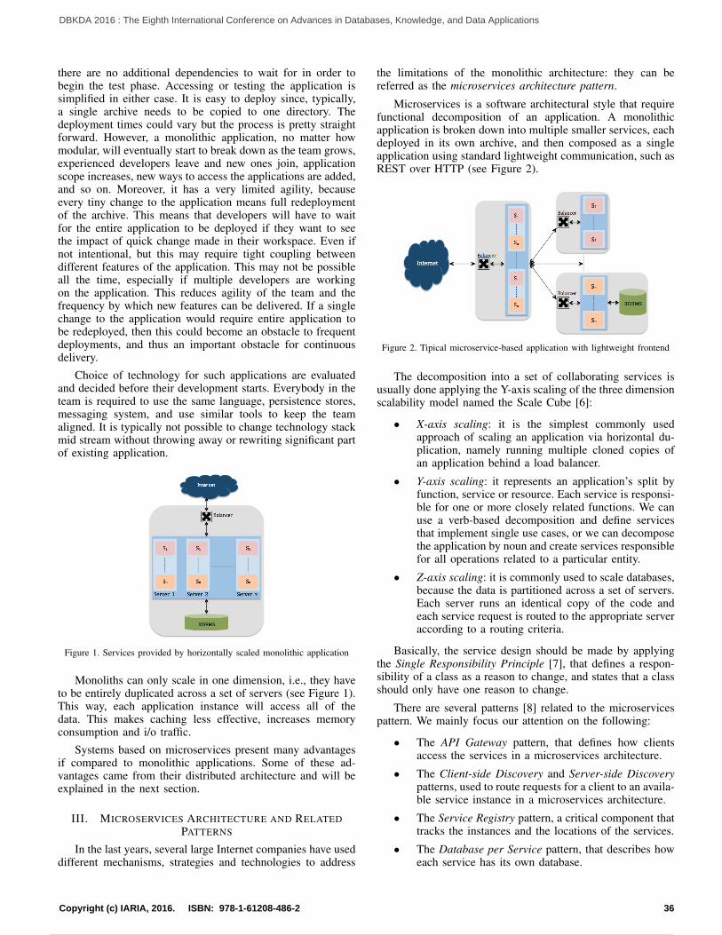
there are no additional dependencies to wait for in order tobegin the test phase. Accessing or testing the application issimplified in either case. It is easy to deploy since, typically,a single archive needs to be copied to one directory. Thedeployment times could vary but the process is pretty straightforward. However, a monolithic application, no matter howmodular, will eventually start to break down as the team grows,experienced developers leave and new ones join, applicationscope increases, new ways to access the applications are added,and so on. Moreover, it has a very limited agility, becauseevery tiny change to the application means full redeploymentof the archive. This means that developers will have to waitfor the entire application to be deployed if they want to seethe impact of quick change made in their workspace. Even ifnot intentional, but this may require tight coupling betweendifferent features of the application. This may not be possibleall the time, especially if multiple developers are workingon the application. This reduces agility of the team and thefrequency by which new features can be delivered. If a singlechange to the application would require entire application tobe redeployed, then this could become an obstacle to frequentdeployments, and thus an important obstacle for continuousdelivery.

Choice of technology for such applications are evaluatedand decided before their development starts. Everybody in theteam is required to use the same language, persistence stores,messaging system, and use similar tools to keep the teamaligned. It is typically not possible to change technology stackmid stream without throwing away or rewriting significant partof existing application.

Figure 1. Services provided by horizontally scaled monolithic application

Monoliths can only scale in one dimension, i.e., they haveto be entirely duplicated across a set of servers (see Figure 1).This way, each application instance will access all of thedata. This makes caching less effective, increases memoryconsumption and i/o traffic.

Systems based on microservices present many advantagesif compared to monolithic applications. Some of these ad-vantages came from their distributed architecture and will beexplained in the next section.

III. MICROSERVICES ARCHITECTURE AND RELATEDPATTERNS

In the last years, several large Internet companies have useddifferent mechanisms, strategies and technologies to address

the limitations of the monolithic architecture: they can bereferred as the microservices architecture pattern.

Microservices is a software architectural style that requirefunctional decomposition of an application. A monolithicapplication is broken down into multiple smaller services, eachdeployed in its own archive, and then composed as a singleapplication using standard lightweight communication, such asREST over HTTP (see Figure 2).

Figure 2. Tipical microservice-based application with lightweight frontend

The decomposition into a set of collaborating services isusually done applying the Y-axis scaling of the three dimensionscalability model named the Scale Cube [6]:

• X-axis scaling: it is the simplest commonly usedapproach of scaling an application via horizontal du-plication, namely running multiple cloned copies ofan application behind a load balancer.

• Y-axis scaling: it represents an application’s split byfunction, service or resource. Each service is responsi-ble for one or more closely related functions. We canuse a verb-based decomposition and define servicesthat implement single use cases, or we can decomposethe application by noun and create services responsiblefor all operations related to a particular entity.

• Z-axis scaling: it is commonly used to scale databases,because the data is partitioned across a set of servers.Each server runs an identical copy of the code andeach service request is routed to the appropriate serveraccording to a routing criteria.

Basically, the service design should be made by applyingthe Single Responsibility Principle [7], that defines a respon-sibility of a class as a reason to change, and states that a classshould only have one reason to change.

There are several patterns [8] related to the microservicespattern. We mainly focus our attention on the following:

• The API Gateway pattern, that defines how clientsaccess the services in a microservices architecture.

• The Client-side Discovery and Server-side Discoverypatterns, used to route requests for a client to an availa-ble service instance in a microservices architecture.

• The Service Registry pattern, a critical component thattracks the instances and the locations of the services.

• The Database per Service pattern, that describes howeach service has its own database.



47 / 107

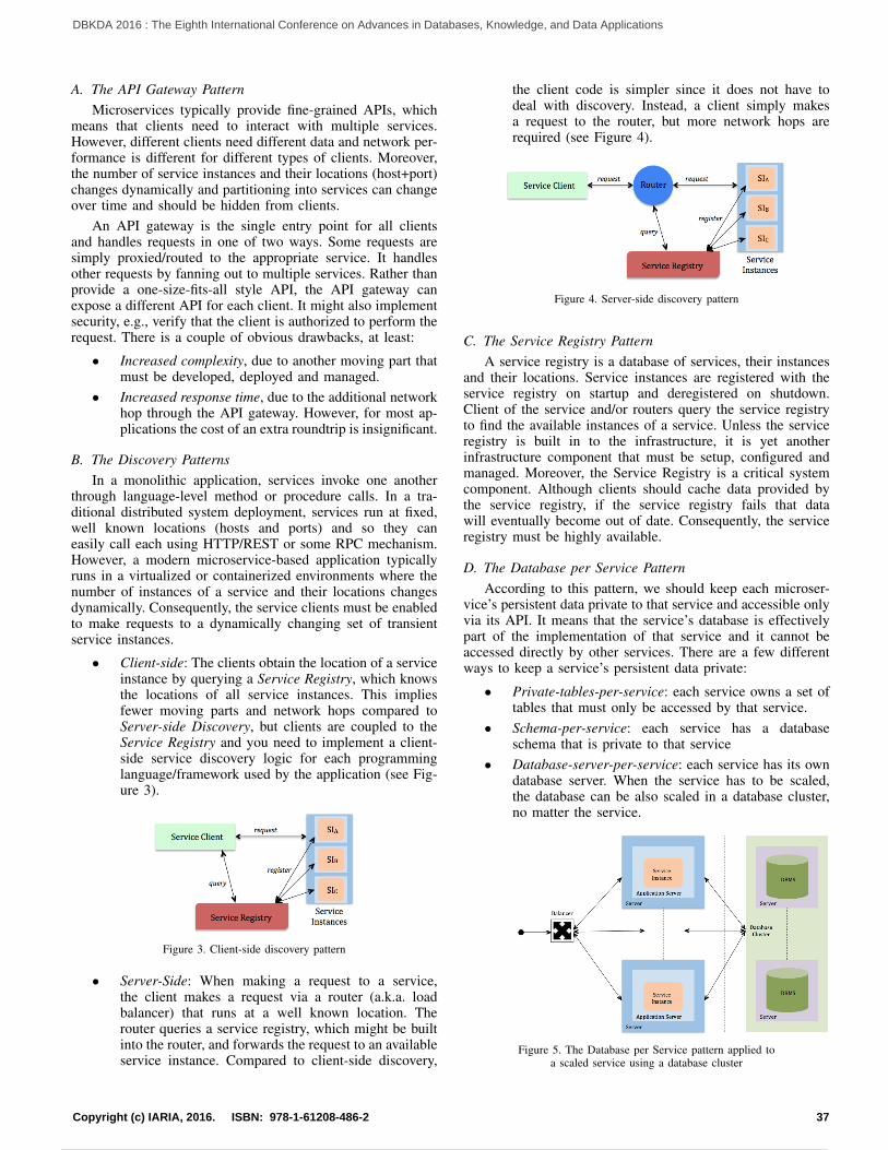
A. The API Gateway PatternMicroservices typically provide fine-grained APIs, which

means that clients need to interact with multiple services.However, different clients need different data and network per-formance is different for different types of clients. Moreover,the number of service instances and their locations (host+port)changes dynamically and partitioning into services can changeover time and should be hidden from clients.

An API gateway is the single entry point for all clientsand handles requests in one of two ways. Some requests aresimply proxied/routed to the appropriate service. It handlesother requests by fanning out to multiple services. Rather thanprovide a one-size-fits-all style API, the API gateway canexpose a different API for each client. It might also implementsecurity, e.g., verify that the client is authorized to perform therequest. There is a couple of obvious drawbacks, at least:

• Increased complexity, due to another moving part thatmust be developed, deployed and managed.

• Increased response time, due to the additional networkhop through the API gateway. However, for most ap-plications the cost of an extra roundtrip is insignificant.

B. The Discovery PatternsIn a monolithic application, services invoke one another

through language-level method or procedure calls. In a tra-ditional distributed system deployment, services run at fixed,well known locations (hosts and ports) and so they caneasily call each using HTTP/REST or some RPC mechanism.However, a modern microservice-based application typicallyruns in a virtualized or containerized environments where thenumber of instances of a service and their locations changesdynamically. Consequently, the service clients must be enabledto make requests to a dynamically changing set of transientservice instances.

• Client-side: The clients obtain the location of a serviceinstance by querying a Service Registry, which knowsthe locations of all service instances. This impliesfewer moving parts and network hops compared toServer-side Discovery, but clients are coupled to theService Registry and you need to implement a client-side service discovery logic for each programminglanguage/framework used by the application (see Fig-ure 3).

Figure 3. Client-side discovery pattern

• Server-Side: When making a request to a service,the client makes a request via a router (a.k.a. loadbalancer) that runs at a well known location. Therouter queries a service registry, which might be builtinto the router, and forwards the request to an availableservice instance. Compared to client-side discovery,

the client code is simpler since it does not have todeal with discovery. Instead, a client simply makesa request to the router, but more network hops arerequired (see Figure 4).

Figure 4. Server-side discovery pattern

C. The Service Registry PatternA service registry is a database of services, their instances

and their locations. Service instances are registered with theservice registry on startup and deregistered on shutdown.Client of the service and/or routers query the service registryto find the available instances of a service. Unless the serviceregistry is built in to the infrastructure, it is yet anotherinfrastructure component that must be setup, configured andmanaged. Moreover, the Service Registry is a critical systemcomponent. Although clients should cache data provided bythe service registry, if the service registry fails that datawill eventually become out of date. Consequently, the serviceregistry must be highly available.

D. The Database per Service PatternAccording to this pattern, we should keep each microser-

vice’s persistent data private to that service and accessible onlyvia its API. It means that the service’s database is effectivelypart of the implementation of that service and it cannot beaccessed directly by other services. There are a few differentways to keep a service’s persistent data private:

• Private-tables-per-service: each service owns a set oftables that must only be accessed by that service.

• Schema-per-service: each service has a databaseschema that is private to that service

• Database-server-per-service: each service has its owndatabase server. When the service has to be scaled,the database can be also scaled in a database cluster,no matter the service.

Figure 5. The Database per Service pattern applied toa scaled service using a database cluster



48 / 107

Figure 5 shows a typical architecture of a scaledservice using its own database cluster.

IV. THE Database is the Service PATTERN

The granular nature of the microservice architectures maybring many benefits, but also comes with the cost of increasedcomplexity.

Breaking a monolith into microservices simplifies eachindividual component, but the original complexity goes to sur-face when, at some point, someone has to put it all together [9].Certainly, there is a sort of law of conservation of complexityin software and, if we break up big things into small pieces,then we push the complexity to their interactions [10].

Moreover, IT complexity in enterprise today continuesto grow at a dizzying rate. Technology innovation, vendorheterogeneity, and business demands are major reasons whyorganizations are exposed to new risks, based on the gapsopened between the options and features of each IT elementand product, and how they are implemented to support a well-defined policy and company strategy. The impact of such risksincreases exponentially by failing to identify the handshakesand correlations of interrelated elements. Products, vendors,and IT layers must work together to prevent potential blackholes: risks related to availability, resiliency and data loss.

It is not hard to understand how microservice architecturesmay amplify such risks, because their distributed nature. More-over, in a monolithic application there was a method call actingas a subsystem boundary, in the microservice architecture wenow introduce lots of remote procedure calls, REST APIsor messaging to glue components together across differentprocesses and servers.

Once we have distributed a system, we have to considera whole host of concerns that we didn’t before. Networklatency, fault tolerance, message serialisation, unreliable net-works, asynchronicity, versioning, varying loads within ourapplication tiers etc.

Starting from the Database-Server per Service Pattern, theaddition of new behaviors and business logic at the databaselevel may be a possible approach to reduce complexity, andthus the related risks, and also to gain improvements in termsof speed and scalability.

Problem: If each scalable service has its own database(cluster), as shown in Figure 5, is there any way to reduce thecomplexity of the architecture and the related risks, while alsogaining more improvements in terms of speed and scalability?

Solution: Whenever the database has an open architectureand provides the necessary hooks to extend its capabilities,then it can embed the business logic that implements thedesired service. The service is strictly coupled to the data,hence this pattern is even stronger than the Database-Serverper Service Pattern, because the database itself acts as abusiness service. As shown in Figure 6, clients requests arerouted via a load balancer, following the guidelines of theServer-side Discovery Pattern.

Some benefits of such approach are immediately clear atfirst sight:

a) the traditional service layer disappears, thanks to the wholeremoval of related hosts and application servers or contain-ers;

Figure 6. The Database is the Service pattern: DBMS with business logic

b) services deployed into the database have instant access todata, accessible at no cost (no third party libraries, nonetwork issues, and so on);

c) less the involved components, less the complexity, theinteractions and the potential risks.

If the database cluster layer is also available to clients, i.e.,thanks to a specific library, we may achieve further simplifica-tion, because clients requests reach directly the service. UnlikeClient-side Discovery Pattern, there’s no need to implementa discovery logic into clients, there isn’t any balancer, andthe cluster layer supplies, at least, the same Service Registrycapabilities. Figure 7 shows the way that super-simplifiedarchitecture looks.

Figure 7. The Database is the Service pattern with client-side cluster support

Drawbacks are also obvious, first and foremost the depen-dency on the chosen database, because the service becomesintegral to, and inseparable from, the database engine. Test anddebug activities must also involve the database because of hisprimary role. For this reason, the database source code mustbe available, an open source product is the obvious choice.

V. PROOF OF CONCEPT

As a proof of concept for the proposed pattern, we haveadded ebXML registry capabilities to a noSQL database,starting from EXPO [19], a prototypal extension for OrientDBderived from eRIC [20], our previous SQL-based ebXMLregistry implemented as web service in Java.

An ebXML registry [15][16] is an open infrastructurebased on XML that allows electronic exchange of businessinformation in a consistent, secure and interoperable way.

The eXtensible Markup Language (ebXML) is a stan-dard promoted by the Organization for the Advancement ofStructured Information (OASIS) and was designed to create



49 / 107

a global electronic market place where enterprises of anysize, anywhere, can find each other electronically and conductbusiness using exchange of XML messages according to stan-dard business process sequences and mutually agreed tradingpartner protocol agreements.

Nowadays, ebXML concepts and specifications are reusedby the Cross-Enterprise Document Sharing (XDS) architecturalmodel [17], defined by Integrating the Healthcare Enterprise(IHE) initiative [18], which is promoted by healthcare profes-sionals and industries to improve the way computer systemsin healthcare share informations.

In the following subsections, we introduce the noSQLdatabase engine we have chosen and we briefly illustrate whatwe have done and some interesting performances results.

A. Brief overview on OrientDBOrientDB [11] is an open source NoSQL DBMS developed

in Java by Orient Technologies LTD and distributed underthe Apache 2 license [14]. It collects features of documentdatabases and graph databases, including object orientation. Ingraph mode, referenced relationships are like edges, accessibleas first-class objects with a start vertex, end vertex, andproperties. This interesting feature let us represent a relationalmodel in document-graph model maintaining the relationships.

OrientDB supports an extended version of SQL, to allowall sort of CRUD (Create, Read, Update and Delete) andquery operations, and ACID (Atomicity, Consistency, Isolation,Durability) transactions, helpful to recover pending documentat the time of crash. It is easily embeddable and customizableand it handles HTTP Requests, RESTful protocols and JSONwithout any 3rd party libraries or components. It is also fullycompliant with TinkerPop Blueprints [12], the standard ofgraph databases. Finally, his feature can be easily customizedand it supports a multi-master distributed architecture, a 2ndlevel shared cache and the other features offered by embeddedHazelcast [13].

B. A multi-model noSQL DBMS as an ebXML RegistryOrientDB is also a customizable platform to build pow-

erful server component and applications: since it containsan integrated web server, it is possible to create server sideapplications without the need to have a J2EE and Servletcontainer. The customizations can be obtained by developingnew Handlers, to build plugins that start when OrientDB starts,or implementing Custom Commands, the suggested best wayto add custom behaviors or business logic at the server side.

The multi-model nature of the OrientDB engine allowsit to support Object data model, too. This model has beeninherited by Object Oriented programming and supports theinheritance between types (sub-types extends the super-types),the polymorphism when you refer to a base class, and the directbinding from/to objects used in programming languages.

The OrientDB Object Interface works on top of theDocument-Database and works like an Object Database: man-ages Java objects directly. This makes things easier for theJava developer, since the binding between Objects to Recordsis transparent. In that context, the Objects are referred asPOJOs: Plain Old Java Objects. OrientDB uses Java reflectionand Javassist [21] to bound POJOs to Records directly. Thoseproxied instances take care about the synchronization between

a POJO and its underlying record. Every time you invoke asetter method against the POJO, the value is early bound intothe record. Every time you call a getter method, the value isretrieved from the record if the POJO’s field value is null. Lazyloading works in this way too.

The ebXML RIM objects are perfect POJOs, because theyare serializable, have a no-argument constructor, and allowaccess to properties using getter and setter methods that followa simple naming convention. They are also fully described bythe standard set of Java XML annotation tags because theyneed to be transferred over the line properly encapsulated usingthe Java Architecture for XML Binding (JAXB) [22]. Thismeans that we can add new custom properties preceded bythe @XMLTransient tag without breaking things. We have usedthose new properties and the related getter and setter methodsto add native OrientDB links between objects, which can betransparently serialized/deserialized by the OrientDB engine intheir enriched form.

This approach has a great impact on the management ofebXML objects:

a) they are still used in the standard way within the client-server SOAP interactions;

b) the binding to the database records is transparent;c) there is no need of extra data class object (DAO) hierarchy

to manage the persistence;d) we are able to make full use of the OrientDB capabilities.

An extension of the OrientdDB OServerCommandAbstractclass has replaced the old Java servlet in the registry requestsmanagement. In particular, the execute() method is invokedat every HTTP request and let us to read the input HTTPstream and to write into the output HTTP stream. This is theplace where we intercept, elaborate and reply to the incomingrequests, by calling the real ebXML registry layer.

Figure 8. EXPO vs eRIC/PostgreSQL

To verify ebXML specifications compliance and to evaluatethe performances, we have run the same ebXML test suitedeveloped with the JAebXR API [23] and then we havecompared the results in some different configurations. Figure 8



50 / 107

shows the interesting performance improvements obtained withEXPO service.

VI. CONCLUSIONS

While monoliths have been the norm for some time,microservices have emerged as an alternative to deal withcertain limitation in monoliths. However, that doesn’t meanthat monoliths are completely obsolete. Just because othersare gravitating to one more than the other, doesn’t mean thatit’s going to be the best decision. Obviously, it’s importantto look at advantages and disadvantages of each and, as muchinformation as possible, to make the aware decision. Keep alsoin mind that, due to the significant architectural differences, adirect comparative quantitative analysis is actually not easy toachieve, but we are working on it.

In this paper, we introduced a new microservice patternwhere the database is the service. The proposed pattern hasbeen tested adding ebXML registry capabilities to a noSQLdatabase. Experimental tests have shown improved perfor-mances of the proposed simplified microservice architecturecompared with SQL-based ebXML registry implemented astraditional Java web service.

REFERENCES[1] M. Fowler, ”Microservices, a definition of this new architectural

term”, URL: http://martinfowler.com/articles/microservices.html [ac-cessed: 2016-02-12].

[2] M. Villamizar, et al., ”Evaluating the monolithic and the microservicearchitecture pattern to deploy web applications in the cloud”, ”ComputingColombian Conference (10CCC), 2015 10th”, 2015, pp. 583–590, DOI:10.1109/ColumbianCC.2015.7333476.

[3] M. Amaral, et al., ”Performance Evaluation of Microservices Architec-tures Using Containers”, ”2015 IEEE 14th International Symposium onNetwork Computing and Applications (NCA)”, 2015, pp. 27–34, DOI:10.1109/NCA.2015.49.

[4] Docker Inc., ”Docker, An open platform for distributed applicationsfor developers and sysadmins”, URL: https://www.docker.com [accessed:2016-02-12].

[5] D. Namiot and M. Sneps-Sneppe, ”On micro-services architecture”,”International Journal of Open Information Technologies”, 2014, vol.2, no. 9, pp. 24–27, ISSN: 2307-8162.

[6] M. Abbott, T. Keeven, and M. Fisher, ”Splitting Applications or Servicesfor Scale”, URL: http://akfpartners.com/techblog/2008/05/08/splitting-applications-or-services-for-scale/ [accessed: 2016-02-16].

[7] R. C. Martin, ”Agile Software Development: Principles, Patterns, andPractices”, Pearson Education, Nov. 2009, ISBN: 978-0-13597-444-5

[8] C. Richardson, ”Microservice architecture patterns and best practices”,URL: http://microservices.io/index.html [accessed: 2016-02-12].

[9] H. Hammer, ”The Fallacy of Tiny Modules”, URL:http://hueniverse.com/2014/05/30/the-fallacy-of-tiny-modules/ [accessed:2016-02-28].

[10] M. Feathers, ”Microservices Until Macro Complexity”, URL:https://michaelfeathers.silvrback.com/microservices-until-macro-complexity [accessed: 2016-02-28].

[11] Orient Technologies LTD, ”OrientDB”, URL: http://orientdb.com [ac-cessed: 2016-02-10].

[12] Apache Software Foundation, ”Apache TinkerPop”, URL:http://tinkerpop.incubator.apache.org [accessed: 2016-02-11].

[13] Hazelcast Inc., ”Hazelcast, the Operational In-Memory ComputingPlatform”, URL: http://hazelcast.com [accessed: 2016-02-10].

[14] Apache Software Foundation, ”Apache License v2.0”, Jan. 2004, URL:http://www.apache.org/licenses/LICENSE-2.0 [accessed: 2016-02-11].

[15] OASIS ebXML Registry Technical Committee, ”RegistryInformation Model (RIM) v3.0”, 2005, URL: http://docs.oasis-open.org/regrep/regrep-rim/v3.0/regrep-rim-3.0-os.pdf [accessed: 2016-02-10].

[16] OASIS ebXML Registry Technical Committee, ”Registry Services andProtocols v3.0”, 2005, URL: http://docs.oasis-open.org/regrep/regrep-rs/v3.0/regrep-rs-3.0-os.pdf [accessed: 2016-02-10].

[17] R. Noumeir, ”Sharing Medical Records: The XDS Architecture andCommunication Infrastructure”, ”IT Professional”, Sep. 2010, Volume:13, Issue: 4, ISSN: 1520-9202, DOI: 10.1109/MITP.2010.123.

[18] Integrating the Healthcare Enterprise (IHE), 2010, URL: http://ihe.net[accessed: 2016-02-17].

[19] A. Messina, P. Storniolo, and A. Urso, ”Keep it simple, fast and scal-able: a Multi-Model NoSQL DBMS as an (eb)XML-over-SOAP service”,”The 30th IEEE International Conference on Advanced InformationNetworking and Applications (AINA-2016)”, IEEE, in press.

[20] A. Messina and P. Storniolo, ”eRIC v3.2: ebXML Registry byICAR CNR”, Technical Report: RT-ICAR-PA-13-03, Dec. 2013, DOI:10.13140/RG.2.1.2108.9124.

[21] JBoss Javassist, ”Javassist (Java Programming Assistant)”, 2015, URL:http://jboss-javassist.github.io/javassist/ [accessed: 2016-02-29].

[22] Java Community Process, ”JSR 222: Java Architecture for XMLBinding (JAXB) 2.0”, 2009, URL: https://jcp.org/en/jsr/detail?id=222[accessed: 2016-02-29].

[23] A. Messina, P. Storniolo, and A. Urso, ”JAebXR: a Java API forebXML Registries for Federated Health Information Systems”, ”DBKDA2015: The Seventh International Conference on Advances in Databases,Knowledge, and Data Applications”, Rome, Italy, May 2015, pp. 33–39,ISBN: 978-1-61208-408-4.



51 / 107

Multidimensional Structures for Field Based Data

A Review of Models

Taher Omran Ahmed

IT Department, College of Applied Sciences,

Sultanate of Oman,

Computer Science Department, Faculty of Science

Aljabal Algharbi University, Azzentan, Libya

e-mail: [email protected], [email protected]

Abstract— The growth in size of geographical data collected by

different types of sensors and used in diverse applications have

led to the adoption of spatial data warehouses (SDW) and

spatial OLAP (SOLAP). Spatial data are represented as either

discrete (objects) or continuous (raster), also called field-based

data. The latter representation deals with data about natural

phenomena that exist continuously in space and time.

Continuity was not taken into account during the early days of

SDW and SOLAP, however, during the last decade there were

attempts to include this concept within SOLAP. In this paper,

we present some of the concepts, issues and discuss the models

proposed to represent spatiotemporal continuity in a decisional

context and attempt to foresee where the research in this area

is heading.

Keywords-Data Warehousing; Field Based Data; Models;

Multidimensional; SOLAP; Spatial Data.

I. INTRODUCTION

Data warehouses rely on multidimensional structures, which are based on the concept of facts or measures and dimensions. Facts are the subject of analysis and they are usually numeric values. Facts are defined by the combination of values (members) of dimensions if a corresponding value exists. Dimensions represent the context in which measures or facts are analyzed. Usually, dimensions are organized in hierarchies composed of several levels; each level represents a level of detail as required by the expected analysis. A hierarchy is a set of variables which represent different levels of aggregation of the same dimension and which are interlinked by a mapping [18]. Traditional data warehouses deal with alphanumeric data; however, most businesses take geographical location seriously when they seek good decisions and hence a large segment of data stored in corporate databases is spatial. It has been estimated that about 80% of data have a spatial component to it, like an address or a postal code [8]. In order to obtain maximum benefits of the spatial component of data, there had been important efforts that led, eventually, to the introduction and implementation of spatial data warehousing (SDW) and spatial OLAP (SOLAP).

Spatial data warehousing has been recognized as a key technology in enabling the interactive analysis of spatial data sets for decision-making support [11][19]. According to [22] a spatial data warehouse is a subject oriented, integrated,

time-variant and non-volatile collection of both spatial data and non-spatial data in support of management’s decision-making process. In plain terms, it is a conventional data warehouse that contains both spatial and non-spatial data where these two types of data complement each other in the support of the decision making process.

OLAP is a tool for analysis and exploration of conventional (alphanumeric) data warehouses. It can also be used for spatiotemporal analysis and exploration. However, the lack of cartographic representations leads to serious limitations (lack of spatial visualization, lack of map-based navigation, and so on) [19]. To overcome these limitations, visualization tools and map-based navigation tools have to be integrated within the conventional OLAP. The result would be a OLAP that can be seen as a client application on top of a spatial data warehouse [2]. The presence of these components would give specialists from multiple disciplines (forestry, public health, transport,…etc.) a new exploration and analysis potential known as Geographic Knowledge Discovery (GKD) [3].

This paper sheds a light on the research carried on spatial OLAP for continuous field data and the different models that have been proposed. In order to achieve our objective, a brief overview of spatial data warehousing is presented in Section 2. The rest of the paper is organized as follows: In Section 3, we discuss the major concepts of several multidimensional models for continuous field data that have been proposed. A comparison between models is presented in Section 4 and we conclude the paper in Section 5.

II. SPATIAL DATA WAREHOUSINGA AND SPATIAL OLAP

A spatial data warehouse contains three types of spatial dimensions; non-spatial, mixed and spatial dimensions.

The first type is a hierarchy containing members that are only located with place names (an address or a postal code) and not represented geometrically. The absence of geometrical representation handicaps the spatiotemporal exploration and analysis but it is still possible for the users to carry out the spatial cognition [13]. The second type is a hierarchy whose detailed level members have a geometric representation but general levels do not have one (at a certain level of aggregation). An example of this type of dimensions is using maps with polygons for cities and regions but neither



52 / 107

for states nor country. In the last type of spatial dimensions, all members have a geometric representation.

In addition to spatial dimensions, two types of spatial measures are also distinguished, the first being a geometric shape or a set of shapes obtained by a combination of several geometric spatial dimensions. The second type is a result of spatial metric or topological operators [20].

A literature review of SOLAP shows an extensive amount of work, unfortunately most of the published research focused on the implementation side and on showing the advantages and potential uses of SOLAP. To the best of our knowledge, there is not enough solid attempts to go in-depth in the theory behind the concepts or to propose a sound mathematical model. Hence, SOLAP remained just an application that can be seen - by many - merely as a coupling between OLAP and GIS. Moreover, SOLAP solely deals with the discrete representation of GIS and hence it cannot grasp the essence of continuity in natural phenomena. Even when continuous field data are dealt with in a decisional context [14] they are treated as discrete and hence they lack their main characteristic that is, spatiotemporal continuity. For instance, [24] proposed a logical model to integrate spatial dimensions representing incomplete field data at different resolutions in a classical SOLAP architecture. Nonetheless, during the last ten or more years, serious attempts were made at integrating continuity in multidimensional structures.

III. MODELS

There is no consensus on one specific model to represent multidimensional structures for field-based data. In fact, even conventional multidimensional structures, which are more established, use different models. Over the last few years, several models were proposed for spatiotemporal multidimensional structures such as [21], where a logical multidimensional model to support spatial data on SDW is proposed. But, most of them concentrate on spatial continuity rather than spatiotemporal continuity.

In this section we present an overview of the main concepts of (four) major models.

A. Ahmed and Miquel, 2005

The model presented in [1] is one of the earliest models for multidimensional structures that attempts to include continuous field data as measures and dimensions. The researchers present the concepts, research issues and potentials of continuous multidimensional structures and propose a model for continuous field data. The model is based on the concept of basic cubes, which are used as the lowest level of detail of dimensions. To imitate the behavior of natural phenomena a continuous data warehouse will be treated as a second layer on top of the discrete data warehouse.

1) Basic Definitions There are n dimensions with r being the rank of

dimension levels starting from (level 1) all the way up to (level r) and k being the cardinality (number of members) of a given dimension level DLi. The domain of values dom(DLi)

for a given dimension level DLi may contain two types of members: predefined members and any possible value between any two given members to give a continuous representation of the dimension level. A value x belonging to a specific dimension level DLi can have ancestors and descendants which are specific instances related to x at higher and lower dimension levels respectively.

2) Basic Cubes A basic cube is a cube at the lowest level of detail. The

discrete basic cube discCb is a 3-tuple <Db, Lb, Rb> where Db is a list of dimensions including a dimension measure M. Lb is the list of the lowest levels of each dimension and Rb is a set of cell data represented as a set of tuples containing level members and measures in the form of x = [x1, x2,...xn, m] where m is the dimension that represents the measure.

To obtain a continuous representation of the basic cube, estimated measures related to the infinite members of a given spatial and temporal levels are calculated using actual cell values from discCb. This involves applying interpolation functions to a sample of discCb values to calculate the measures corresponding to the new dimension members, which will result in continuous basic cube contCb.

A continuous basic cube contCb is 4-tuple <Db, (D’b, F), Lb, R’b>. Discrete and continuous dimensions are represented by Db, D’b respectively. In addition, F is a set of interpolation functions associated with the continuous dimensions and has the same cardinality as D’b. The lowest levels of dimensions are represented by Lb. The continuous representation is defined over a spatial and/or temporal interval. Hence, R’b is a set of tuples of the form x = [x1,

x2,… xn, m] where xi ∈ [minDom(Lbi) - , maxDom(Lbi)+

] with being a small predefined value used to allow for continuous representation around the values of the domain of the dimension levels, and to predict values outside the specified interval. The measure m ⊆ M can be either interpolated (approximated) or exact. When measures are interpolated m is defined as: m= f(m1, m2,…,mk) where ƒ is a spatial or temporal

interpolation function,

m= f(m1, m2,…,mk) using values lying within a

predefined spatial or temporal distance d, or

m = f1 o f2 (m1, m2,…,mk) or m = f2 o f1 (m1, m2,…, mk).

The order of applying interpolation functions.

It can be concluded that discCb contCb

3) Cubes Cubes at higher levels are built by applying a set of

operations on data at the basic cube level. A cube C is defined as 4-tuple <D, L, contCb, R> where, D is a list of dimensions including M as defined before, L is the respective dimension level, R is cell data and contCb is the basic cube from which C is built. Because of the nature of the continuous field data, different aggregation functions are used to build the cube at higher dimension hierarchies. For example, the sum of measures for a specific region or a specific period will be represented as an integral. Other aggregation functions like min, max or average will be



53 / 107

performed on contCb and their results will be assigned to the higher levels of the hierarchy.

4) Aggregations On a continuous field, two classes of operations are

defined. The first deals with discrete operations and the second groups the continuous operations:

Discrete operations. Only the sample points are used.

DiscMax = vi such that vi ≥ f(sk) ∀ sk ∈ S

DiscMin = vi such that vi ≤ f(sk) ∀ sk ∈ S

DiscSum =

DiscCount = Card(S)

DiscAvg =

Continuous operations. All values of the field are used.

ContMax = vi such that vi ≥ f(Sk) ∀ Sk ∈ D × T

Cont Min = vi such that vi ≤ f(Sk) ∀ Sk ∈ D × T

ContSpatSum =

ContTempSum=

ContSpatAvg=

ContTempAvg = where [t1:t2] is a time interval

B. Vaisman and Zimányi, 2009

Vaisman et al. [23] base their multidimensional model for continuous fields in spatial data warehouses on MultiDim model presented in [12]. A multidimensional schema consists of a finite set of dimensions and fact relationships. A dimension consists of at least one hierarchy, containing at least one level. A basic hierarchy is hierarchy with only one level. Several levels are related to each other through a

binary relationship that defines a partial order between

levels. For any two consecutive related levels li, lj, if li lj then li is called child and lj is called parent. A level representing the less detailed data for a hierarchy is called a leaf level.

For spatial levels, the relationship can also be topological requiring a spatial predicate, e.g., intersection. A fact relationship may contain measures that can be spatial or thematic. The thematic measures are numeric that are analyzed quantifiably whereas the spatial measure can be represented by a geometry or field, or calculated using spatial operators, such as distance or area.

The dimension levels have two types of attributes (category and property). For parent level, the category attribute defines how child members are grouped. In the leaf level, the category attribute indicates the aggregation level of

a measure in the fact relationship. The property attribute can be spatial (represented by geometry or field) or thematic (descriptive, alphanumeric data types). Hence, property attribute provides additional features of the level. A level is spatial if it has at least one spatial property attribute. Likewise, a hierarchy is spatial if it has at least one spatial level.

A field type is defined as a function from the spatial domain to a base type. Field types are obtained by applying the field(.). Therefore, the result of field(real) (e.g. representing a natural phenomenon) is a continuous function f : point → real. There are two types of fields (temporal and nontemporal). Field types are partial functions, i.e., they may be undefined for certain regions of space. Along with field types a set of operations over fields are defined and classified as in Table 1.

TABLE I. FIELDS AND OPERATION SETS

Class Operations

Projection to

Domain/Range defspace, rangevalues, point, val

Interaction with

Domain/Range

atpoint, atpoint, atline, atregion, at, atmin,

atmax, defined, takes, concave, convex, flex

Rate of change partialder_x, partialder_y

Aggregation operators

integral, area, surface, favg, fvariance, fstdev

Lifting Operations on discrete types are generalized for

field types

1) Relational Calculus To express SOLAP queries [23], use a query language

based on the tuple relational calculus (as in [7]) extended with aggregate functions and variable definitions. They show that this language expresses standard SOLAP queries and that, by extending the calculus with field types multidimensional, queries over fields can be expressed. The query language is introduced by example.

Figure 1 and Figure 2 show a query over discrete data and SOLAP operations respectively.

Figure 1. Query over discrete data

Figure 2. SOALP operations



54 / 107

2) Extending OLAP Operations with Continuous Fields In addition to operations defined on fields specified in

3.2.1, they also define another set of operations that allows the interaction with domain and range. These operations are listed in Figure 3.

atpoint, atpoints, atline, atregion

restrict the function to a given subset of the space defined by a spatial value.

at : restricts the function to a point or to a point set (a range) in the range of the function.

concave, convex:

restrict the function to the points where it is concave or convex, respectively

flex : restricts the function to the points where convexity changes

Figure 3. Domain and range operators

There are also operators to compute how the field changes in space. Moreover, there are three aggregate operators defined as follows:

Field average favg : integral/area

Field variance fvariance : dxdy

Field Standard deviation fstdev : A class of multidimensional queries over fields denoted

SOLAP-CF queries is also defined. Fields are classified as

temporal identified by f( , ) pictogram and Non-temporal

identified by f( ) pictogram. In the Non-temporal field, each point in the space has a value (e.g., soil type) whereas for temporal field there is a value that changes with time instant at each point in the space (e.g. temperature). The model also supports field measures that can be pre-computed in the pre-processing stage as a function of many factors.

C. Bimonte and Kang, 2010 Prior to introducing their model, Bimonte et al. [4] define

four requirements for definition of a formal model for field data as dimension and measures:

1. Measures as continuous field data 2. Hierarchy on continuous field data 3. Aggregation functions as Map Algebra functions 4. Independence of implementation They argue that no existing model satisfies all 4

requirements.

1) Definitions As in the previous models, Bimonte et al. [4] start by

providing a uniform representation for field and vector data, which are used to define measures and dimensions members of the multidimensional model.

Real world entities are represented by 3 types of objects described by alphanumeric attributes. An object can represent levels and members of dimensions.

a) An object

An Object Structure Se is a tuple ⟨a1 …an⟩ where i

[1,…n] ai is an attribute defined on a domain dom(ai)

An Instance of an Object Structure Se is a tuple

⟨val(a1),…val(an)⟩ where i [1,…n], val(ai) dom(ai)

'I(Se)' denotes the set of instances of Se

b) Geographic Object A geographic object is a geometry (geom) and an optional

set of alphanumeric attributes ([a1, … an]) whose values are

associated to the whole geometry according to the vector

model. Let g R2. An Object Structure Se = ⟨geom, [a1,… an]⟩ is a

Geographic Object Structure if the domain of the attribute

geom is a set of geometries: dom(geom) 2g

geom is called 'geometric support'

c) Field Object A Field Object extends a Geographic Object with a function that

associates each point of the geometry to an alphanumeric value.

Let Se = ⟨geom, field, [a1,… an]⟩ a Geographic Object

Structure. Se is a Field Object Structure if the domain of

the attribute field is a set of functions defined on m sub-

sets of points of geom having values in an alphanumeric

domain domfield : dom(field)= {f1 … fm}

An Instance of a Field Object Structure Se is a tuple ⟨g,

fj, val(a1),…val(an)⟩ where:

- i [1,…n] val(ai) dom(ai), g dom(geom)

- fj : g → domfield and fj {f1 , …, fm}

'field support' is the input domain of fj

2) Spatio-multidimensional Model for Field Data A spatio-multidimensional model uses data as

dimensions composed of hierarchies, and facts described by measures. A hypercube is an instance of the spatio-multidimensional model.

a) Hierarchies and facts

Vector objects are organized in a hierarchical way. A Spatial Hierarchy organizes the Geographic Objects into a hierarchy structure using a partial order ≤h where Si ≤h Sj means that Si is a less detailed level than Sj. Measures are aggregated according to the groups of spatial members defined by the tree <h.

Field Hierarchy is defined as a hierarchy of field objects.

A Field Hierarchy Structure, Hh, is a tuple ⟨Lh, h, h, ≤h⟩ where:

- h, h, are of Field Object Structures, and Lh is a set of

Field Object Structures - ≤h is a partial order defined on Lh, h, h.

An Instance of a Field Hierarchy Structure Hh is two

partial orders: <h and <f such that: - <h is defined on the instances of h, h, h. Noted as

<h 'geographic objects order'



55 / 107

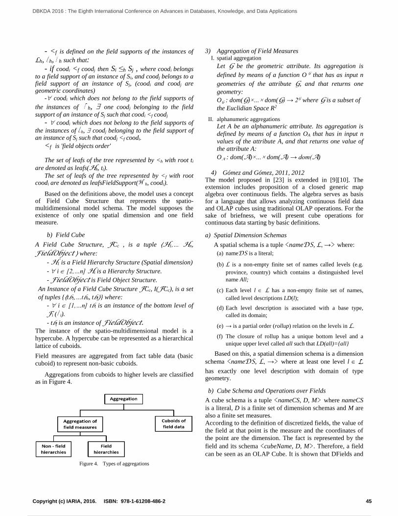
- <f is defined on the field supports of the instances of

Lh, h, h such that: - if coodi <f coodj then Si ≤h Sj , where coodi belongs

to a field support of an instance of Si, and coodj belongs to a field support of an instance of Sj, (coodi and coodj are geometric coordinates)

- coodi which does not belong to the field supports of

the instances of h, one coodj belonging to the field

support of an instance of Sj such that coodi <f coodj

- coodi which does not belong to the field supports of

the instances of h, coodj belonging to the field support of an instance of Sj such that coodj <f coodi.

<f is 'field objects order'

The set of leafs of the tree represented by <h with root ti

are denoted as leafs(Hh, ti).

The set of leafs of the tree represented by <f with root coodi are denoted as leafsFieldSupport( h, coodi).

Based on the definitions above, the model uses a concept of Field Cube Structure that represents the spatio-multidimensional model schema. The model supposes the existence of only one spatial dimension and one field measure.

b) Field Cube

A Field Cube Structure, FCc , is a tuple ⟨H1,… Hn,

FieldObject ⟩ where:

- H1 is a Field Hierarchy Structure (Spatial dimension)

- i [2,…n] Hi is a Hierarchy Structure.

- FieldObject is Field Object Structure.

An Instance of a Field Cube Structure FCc, I(FCc), is a set

of tuples {⟨tb1,…tbn, tbf⟩} where:

- i [1,…n] tbi is an instance of the bottom level of

Fi ( i).

- tbf is an instance of FieldObject. The instance of the spatio-multidimensional model is a

hypercube. A hypercube can be represented as a hierarchical

lattice of cuboids.

Field measures are aggregated from fact table data (basic

cuboid) to represent non-basic cuboids.

Aggregations from cuboids to higher levels are classified as in Figure 4.

Figure 4. Types of aggregations

3) Aggregation of Field Measures I. spatial aggregation

Let G be the geometric attribute. Its aggregation is

defined by means of a function O G that has as input n

geometries of the attribute G, and that returns one

geometry:

OG : dom(G)×…× dom(G) → 2G where G is a subset of

the Euclidian Space R2

II. alphanumeric aggregations

Let A be an alphanumeric attribute. Its aggregation is

defined by means of a function OA that has in input n

values of the attribute A, and that returns one value of

the attribute A:

OA : dom(A)×…× dom(A) → dom(A)

4) Gómez and Gómez, 2011, 2012 The model proposed in [23] is extended in [9][10]. The extension includes proposition of a closed generic map algebra over continuous fields. The algebra serves as basis for a language that allows analyzing continuous field data and OLAP cubes using traditional OLAP operations. For the sake of briefness, we will present cube operations for continuous data starting by basic definitions.

a) Spatial Dimension Schemas

A spatial schema is a tuple <nameDS, L, →> where:

(a) nameDS is a literal;

(b) L is a non-empty finite set of names called levels (e.g.

province, country) which contains a distinguished level

name All;

(c) Each level l L has a non-empty finite set of names,

called level descriptions LD(l);

(d) Each level description is associated with a base type,

called its domain;

(e) → is a partial order (rollup) relation on the levels in L.

(f) The closure of rollup has a unique bottom level and a

unique upper level called all such that LD(all)={all}

Based on this, a spatial dimension schema is a dimension

schema <nameDS, L, →> where at least one level l L

has exactly one level description with domain of type geometry.

b) Cube Schema and Operations over Fields

A cube schema is a tuple <nameCS, D, M> where nameCS

is a literal, D is a finite set of dimension schemas and M are

also a finite set measures.

According to the definition of discretized fields, the value of

the field at that point is the measure and the coordinates of

the point are the dimension. The fact is represented by the

field and its schema <cubeName, D, M>. Therefore, a field

can be seen as an OLAP Cube. It is shown that DFields and



56 / 107

traditional OLAP cubes can be easily integrated for data

analysis.

They also define a set of aggregate functions A = {Max,

Min, Avg, Sum}.

Dice operator. This operation selects values in

dimensions or measures based on a Boolean condition which may introduce discontinuity. To avoid discontinuity,

the operator is defined by setting the value of samples with

values where the operator is not satisfied.

ROLL-UP operator. It aggregates facts according to dimension hierarchy. In this model the spatial dimension is a single-level dimension which implies that rollup hierarchies must be introduced externally. Three roll-up operations are defined (spatial over spatial field, spatial over spatiotemporal field and temporal over spatiotemporal fields).

Drill-Down. This operations aggregates facts according to dimension hierarchy. In this model, the spatial dimension is a single-level dimension which implies that rollup hierarchies must be introduced externally. They define 3 roll-up operations (spatial over spatial field, spatial over spatiotemporal field and temporal over spatiotemporal fields).

Roll-Up. This operation reverses the effect of Roll-Up so it is just the inverse of the mentioned operator.

IV. DISCUSSION

The approaches used in the above listed proposals (and in others) are diverse to say the least. Moreover, it seems that there is no build up on previous work or any attempts to criticize or enhance what has already been done which leads to a plethora of models without a clear attempt to define a mainstream model.

To compare the 4 models, one needs to define criteria and search which model meets the necessary requirements to become an applicable model. According to [6], true data models should have 3 components: A structure that defines how data are structured, integrity rules that define how data are kept correct and consistent and operators which define how data are manipulated. Therefore we will compare these models using the above mentioned conditions in addition to the requirements defined by [4] and additional requirements defined in [16][17]. The different models are evaluated against these six requirements (Table 2):

1) Structure

The common structure between all models is the hypercube.

Each model proposes a different way of building its

hypercube.

2) Integrity rules

Multidimensional structures are not concerned with integrity

as much as they are concerned with fast response to

analytical queries.

3) Operators

This complexity of SOLAP queries implies long query

processing time. Therefore, most queries are run in advance

and the results are stored as materialized views. Operators

are either for navigation along the analysis dimensions or

for returning previously computed results.

4) Continuous data as measures

Usually measures are numerical values that are analyzed

according to axis of analysis (the dimensions). In the models

we reviewed only one proposal imposes continuous data as

measures constraint.

5) Explicit hierarchies in dimensions The hierarchy should be explicit to allow the user to

navigate with clear knowledge of the relationship between

the different levels [15].

6) Symmetric treatment of dimensions and measures: Since measures can be a level of a dimension, it is

essential that measures can be transformed into attributes and vice versa [5]. This will provide an important functionality to any OLAP system.

TABLE II. MULTIDIMENSIONAL MODEL COMPARISON CRITERIA

To clarify some of the differences between the 4 models,

we will present examples of how the aggregate average is

handled by each model.

In [1], to find the average pollution for a specific region,

the aggregation is done by applying interpolation functions

to the basic cubes to obtain a continuous representation of

the field. The sum of all values is calculated as in integral of

the function representing the field. The average is then

obtained by dividing the sum by the area of the field. In

[23], the average monthly temperature for a land plot is

calculated as follows :

{l.number, m.month, temp | LandPlot(l) ^ Month(m)^

first=min({t.date|Time(t) ^ t.month = m.id}^last=

max({t.date|Time(t)^t.month=m.id}^ temp = avg

({atperiods (atregion(t.geometry,l.geometry), range(first,

last)) | Temperature(t)})} Where first and last represent

first and last day of the month.

Criteria Ahmed

et al. [1]

Vaisman

et al. [23]

Bimonte

et al. [4]

Gómez et

al. [9][10]

Structures

Integrity rules x x x x

Operators

Continuous data

as measures x x x

Explicit

hierarchies x x

Symmetric

treatment of

dimensions and

measures

x x x



57 / 107

In [4], the aggregation is performed by applying the

average on the Field Hierarchy Hregres.

F4(x;y)=AVG(leavesFieldSupport(Hdeptres, (x2;y2))) =

AVG(f3(x;y), f3(x1;y1)).

For more details about the examples we refer the reader to

[1][4][9][23].

From Table 2, none of the proposed models satisfies all

criteria. Models proposed by Vaisman et al. [23] and Gómez

et al. [9][10] satisfy only structure and operators constraints.

The major weakness is the lack explicit hierarchies, which is

essential for navigation in cubes. The model presented by

Ahmed et al. [1] lacks treatment of continuous data as a

measure which is supported in [4]. However, Bimonte et al.

[4] does not treat dimensions and measures symmetrically.

V. CONCLUSION

Spatial data warehouses have been around for some time now. Most of the early work on this topic was oriented towards discrete spatial data. The combination of cartographic display and OLAP resulted in SOLAP. However it was also limited to discrete spatial representation. Attempts at integrating continuous or field based data in multidimensional structures began about 10 years ago. During this period, a number of models to represent spatial and/or spatiotemporal continuity were proposed. In this paper, we studied some of these models and compared them with respect to different criteria and conditions for multidimensional models. None of the different proposals covered all comparison criteria and hence there is still a considerable amount of work to be done on the subject. The other remark is that most of the work concentrated on the theoretical side without a mention of solid model that can be used in real life application. To the best of our knowledge, even though there is still an undiscovered wealth mine for research and development, there is a lack of recent work on this domain.

REFERENCES

[1] T. O. Ahmed and M. Miquel. “Multidimensional Structures Dedicated to Continuous Spatiotemporal Phenomena”. In proceedings of the 22nd British National Conference on Databases (BNCOD), (Sunderland, UK, July 5-7, 2005) 29-40.

[2] T. O. Ahmed. “Spatial On-line Analytical Processing (SOLAP): Overview and Current Trends”. In proceedings of Internationa Conference on Advanced Computer Theory and Engineering (ICACTE), (Phuket, Thailand, December, 20-22, 2008) 1095-1099.

[3] Y. Bédard, T. Merrett and J. Han. “Fundamentals of Spatial Data Warehousing for Geographic Knowledge Discovery in Geographic Data Mining and Knowledge Discovery”. Research Monographs in GIS Series. Edited by Peter Fisher and Jonathan Raper. 2001. 53-73.

[4] S. Bimonte and M. A. Kang. “Towards a Model for the Multidimensional Analysis of Field Data”. In proceedings of the 14th East European Conference (ADBIS10) (Novi Sad, Serbia, Sep 20-24, 2010. 300-311.

[5] L. Cabibbo and R. Torlone. “From a procedural to a visual query language for OLAP”. In proceedings of the 10th International Conference on Scientific and Statistical

Database Management (SSDBM’98), IEEE Computer Society Press, Washington, DC, USA pp. 74–83, 1998.

[6] E. F. Codd. “Data Models in Database Management”. ACM SIGMOD Record 11(2), 1981, pp. 112-114.

[7] R. Elmasri. and S. Navathe. Fundamentals of Database Systems. Pearson, 7th edition, 2015.

[8] C. Franklin. “An Introduction to geographic Information Systems: Linking Maps to databases”. Database, 1992. pp. 13-21.

[9] L. Gómez, S. Gómez and A. Vaisman. “Analyzing Continuous Fields with OLAP Cubes”. In proceedings of the 14th Workshop DOLAP (DOLAP’11), (Glasgow, Scotland, Oct 24-28, 2011). pp. 89-94

[10] L. Gómez, S. Gómez and A. Vaisman. “A Generic Data Model and Query Language for Spatiotemporal OLAP Cube Analysis”. In proceedings of the 15th International Conference on Extending Database Technology (EDBT2012) (Berlin, Germany) Mar 27-30, 2012, pp. 300-311.

[11] J. Han, R. Altman, V. Kumar, H. Mannila and D. Pregibon. “Emerging Scientific Applications in Data Mining”. Communication of the ACM, 45,8 (Aug 2002), pp. 54-58.

[12] E. Malinowski and E. Zimányi. “Advanced Data Warehouse Design: From Conventional to Spatial and Temporal Applications”. Data-Centric Systems and Applications, Springer, 2008.

[13] P. Marchand, A. Brisebois, Y. Bedard and G. Edwards. “Implementation and Evaluation of a Hypercube-Based Method for Spatiotemporal Exploration and Analysis”. ISPRS Journal of Photogrammetry and Remote Sensing. (Aug 2004) 59(1-2), pp. 6-20.

[14] F. Moreno, J. A. E. Arias and B. M. Losada. “A Conceptual Spatio-temporal Multidimensional Model”. Revista Ingenierías Universidad de Medellín. (2011) 9(17), pp. 175-184.

[15] T. B. Pederson. “Managing complex multidimensional data”. Business Intelligence: Lecture Notes in Business Information Processing. (2013) vol. 138. pp. 1-28.

[16] T. Pedersen and C. Jensen. “Multidimensional Data Modeling for Complex Data”. In proceedings of the 15th International Conference on Data Engineering (ICDE99)(Sydney, Australia) March 23-26 1999, pp. 336-345.

[17] G. Pestana and M. Mira da Silva. “Multidimensional Modeling based on Spatial, Temporal and Spatio-Temporal Stereotypes”. 5th ESRI International User Conference (ESRI) (San Diego, USA) Jul 25-29, 2005, pp. 5-15.

[18] E. Pourabbas and M. Rafanelli. “Characterization of Hierarchies and Some Operators in OLAP Environment.” In proceedings of the 2nd ACM International Workshop on Data Warehousing and OLAP. (Kansas City, USA). Nov 2-6, 1999, pp. 54 - 59.

[19] S. Rivest, Y. Bedard and P. Marchand. “Towards better Support for Spatial Decision Making: Defining the Characteristics of Spatial On-Line Analytical Processing (SOLAP)”. Journal of Canadian Institute of Geomatics, 55(4), 2001, pp. 539-555.

[20] S. Rivest, Y. Bedard, M. J. Proulx and M. Nadeau. “SOLAP: A New Type of User Interface to Support Spatiotemporal Multidimensional Data Exploration and Analysis”. In proceedings of ISPRS workshop on Spatial, Temporal and Multi-Dimensional Data Modeling and Analysis, (Québec, Canada) Oct 2-3, 2003.

[21] M. Sampaio, A. Sousa and C. Baptista. “Towards a Logical Multidimensional Model for Spatial Data Warehousing and OLAP”. In proceedings of 9th ACM International Workshop on Data Warehousing and OLAP (New York, USA) Nov 5-11, 2006, pp. 83-90.



58 / 107

[22] N. Stefanovic, J. Han and K. Koperski. “Object-based Selective Materialization for Efficient Implementation of Spatial Data Cubes”. IEEE Transactions on Knowledge and Data Engineering, (Nov-Dec 2000) 12(6), pp. 938 – 957.

[23] A. A. Vaisman and E. Zimányi. “A Multidimensional Model Representing Continuous Fields in Spatial Data Warehouses”. In proceedings of the International Conference on Advances in Geographic Information Systems (ACM SIGSPATIAL GIS 2009)(Seattle, USA) Nov 4-6, 2009, pp. 168-177.

[24] M. Zaamoune, S. Bimonte, F. Pinet and P. Beaune. “A New Relational Spatial OLAP Approach for Multi-resolution and Spatio-multidimensional Analysis of Incomplete Field Data”. In proceedings of International Conference on Enterprise Information Systems (ICEIS 2013)(Angers, France) 4-7 Jul 2013, pp. 145 -152.



59 / 107

Some Heuristic Approaches for Reducing Energy Consumption on Database

Systems

Miguel Guimarães João Saraiva Orlando Belo ALGORITMI R&D Center

University of Minho Portugal

[email protected]

HasLab R&D Center INESC/University of Minho

Portugal [email protected]

ALGORITMI R&D Center University of Minho

Portugal [email protected]

Abstract—Today, one of the major concerns of administrators and managers of data centers is related with the cost of the energy that each database component consumes when involved in activities and processes they manage. In fact, it is not necessary to conduct a detailed assessment to realize that the cost of energy consumed in this type of systems is really great. So, it is not surprising the significant growing interest that researchers have in this domain. Various techniques have been developed to assess the energy consumption on database systems, demonstrating their utility in managing the power they use to consume. Basically, they come to confirm the paradigm shift on the issue of energy concern in database systems towards the reduction of its consumption. In this paper, we present and discuss a set of heuristics that we suggest to reduce, in particular, the energy consumption on the execution of a given query inside a relational database system. With this work, we intend to contribute to design and implement more efficient queries in terms of energy, i.e., green queries, based on the analysis of the various components that are used in their physical implementation, reducing as much as possible their energy consumption, taking into consideration the characteristics of the database operators used and the querying execution plans established for them.

Keywords-data centers; database management systems; querying execution plans, database queries consumption, green queries; consumption heuristics.

I. INTRODUCTION The assessment of energy consumption of any component

is not an easy task. To carry out appropriately this kind of evaluation, it is necessary to study in detail how the component behaves and how it is used in practice. The same may be applied to the study of power consumption of a DataBase Management System (DBMS) or, in particular, of any query that can be performed in its environment [1]. Any process for the establishment of energy-efficient queries, usually recognized as green queries, and not its optimization in terms of processing time or usage of computing resources, requires a fairly deep knowledge of how queries are processed and optimized in the environment of a DBMS.

Database querying processing [2][3] is one of the most important activities of a DBMS, which involves a well-defined set of processes for supporting the way the system responds to users’ queries. Optimizing querying processing is something that has been worked over the years by researchers in the databases field. See, for example, the work of Ceri and Gottlob [4] that presented a way to transform a SQL statement into relational algebra expressions representing equivalent SQL sub statements, a method revealed by Taniar [5] especially oriented to add additional instructions (e.g., optimizer hints, access method hints, or table joins hints) into SQL statements to instruct the SQL optimizer for executing the statement in an alternative better way, or how Li et al. [6] suggested a manner to improve querying performance with configuration options – e.g., table partitioning, materialized views, or storing plan outlines – increasing as well the efficiency of the code application.

However, as the number and capacity of data centers increases, beside the so usual issues of performance and querying processing abilities – always critical aspects for any DBMS –, the issue of power consumption is appearing very clear in their cost operational reports, year after year [7]. This caught the attention of data centers’ managers all over the world up sharply their concerns related to energy consumption, not only because of the cost of electricity itself but also because of relevant environmental issues. In general, database servers are the biggest customers of computational resources of a conventional data center, which makes them also one of its biggest energy consumers [8]. Although these systems are very well equipped today, with powerful tools for querying optimization, quality of service, or overall performance, usually in terms of energy consumption DBMS do not have any means especially oriented to the management and control of consumption power. With the current trends and needs of the markets and DBMS users, this lack is considered quite serious. The non-availability of data about the energy consumption of a DBMS has been motivating a large diversity of research initiatives aiming to create means so that we can in addition



60 / 107

to defining query optimization plans in DBMS environments also create energy consumption plans for executing queries.

In a previous work [9], we developed a study that allowed us to develop an energy consumption plan for a query that is usually executed in a conventional data center environment. At that time, the goal was reducing, as much as possible, the energy consumption of data centers queries without affecting their usual performance. We believed that such small reduction in the consumption of a simple query could be a great help in reducing the overall consumption of a data center – that was proved easily by multiplying these tiny savings by the huge number of queries (and transactions) that are executed per minute in a data center. Continuing this work, we studied a set of specific heuristics that we suggest to reduce, in particular, the energy consumption on the execution of a given query inside a relational DBMS, which we expect that contribute to design and implement more efficient queries in terms of energy – green queries.

In this paper, we present and discuss the referred energy consumption heuristics, giving particular attention to other related works (Section II), showing how we categorized the energy consumption of a SQL query, what kind of transformation rules were applied, and how the energy was consumed by each one of the transformation rules studied (Section III). Finally, we finish this paper with some brief conclusions and pointing out some future research lines (Section V).

II. RELATED WORK Today, energy efficiency is a trend topic in terms of

researching and development. Researchers of different fields of expertise work and discuss possible solutions to solve the energy crisis that we are facing today. On the one hand, saving energy allow us to reduce the energy billing costs; and on the other hand, by doing that, we are also preserving environment resources. Thus, saving energy and creating policies to develop green software is beneficial for everybody. Steps towards that direction have been already made. At software level, for instance, the works presented in [10] and [11] are some good examples of techniques and methods used to detect energy consumption. In [10], the authors adapted a technique known as Spectrum-based Fault Localization to identify parts of code responsible for a higher energetic consumption. The work done in [11] focused more on finding and detecting anomalous energy consumption in Android systems. Both works show us that reducing energy consumption has been tackled in a variety of systems by several researches, and its popularity in computer science domains has increased.

Database systems have also taken small steps towards green guidelines. The Claremont report was one of the first approaches concerning energy consumption in database systems [12]. The main goal of this report was to take into consideration, during the devise and implementation stages

of a database system, the energy consumed by different tasks. Reinforcing such concerns, the work presented in [13] provided us a clear survey of how to control efficiently energy in data management operations. Later, other studies emerged approaching the same topic [14][15][16]. However, most of them have focus essentially on hardware questions. In terms of software, in [9] it was redesigned the execution plan of a DBMS in order to include, not only the default estimative values for query execution, but also an estimative of energy that will be consumed to run a specific query. Later, it was proposed a solution to redesign a DMBS kernel, in order to reduce energy consumption [15]. Afterward, in [17] other alternatives were suggested to reduce the high levels of energy consumption in DBMS, in general terms, while other works, were concerned about the prediction of the consumption of large join queries [18], or how to optimize queries to reduce global consumption of energy within a DBMS [19]. However, as far as we know, there are no works approaching the effect of regular querying optimization heuristics on the consumption of energy of a DBMS. Thus, we selected some of the most used heuristics on relational querying processing and studied their effect in terms of energy consumption.

III. ENERGY CONSUMPTION CATEGORIZATION The energy consumption paradigm has been increasing

its importance over the last few years, slowly replacing the performance paradigm, in terms of main concerns, to take into account when developing any kind of database querying task. Query processing is one of the most important activities performed by a DBMS. Today, it is possible to analyze and optimize the cost of a database query in terms of performance, establishing better execution plans and reducing querying processing time. Having access to these plans, we can also measure the energy that database operations consume in a similar way as we can measure their processing time. We only need appropriate tools.

A. Data and Test Configuration

In this work, we developed a tool with the ability to measure the energy consumption of SQL queries, categorizing which ones are green and which ones are not. We used the tool gSQL, shorten for greenSQL, to categorize the energy consumption of SQL queries. This tool uses as support the jRAPL framework, which allows for monitoring the energy consumption of different hardware levels for a certain code block [20]. In order to use jRAPL, there are certain conditions that must be fulfilled. The processor has to be from Intel architectures and support Machine-Specific Registers (MSR). The later are the registers used for storing the energy consumption information for code block that was monitored. Therefore, the role played by the jRAPL framework is exclusively dedicated to categorize and analyze the energy consumption of SQL queries. Regarding the gSQL tool, even though its use is simple, it gives us the required information to devise hypothesis and thus create



61 / 107

heuristics to reduce the queries energy consumption. To run the tests it is necessary to specify three different parameters:

1) an input file, with all the queries that going to be tested;

2) the number of times each query will be repeated; 3) the number of times each test will be repeated.

In Figure 1, it is possible to see a brief description of the overall behavior of the gSQL tool, written in pseudo code. After all the tests have been executed, we obtain as result the energy and the time consumption for each query tested. The calculated aggregated values were maximum, minimum, average, and standard deviation. This set of aggregated values allows for us to find out if a certain test need to be executed again, by analyzing the standard deviation as well as the amplitude between maximum and minimum values. For the test environment, we choose the PostgreSQL DBMS, populated with data based on the TPC-H benchmark. Depending on the scaling factor, the database can assume different dimensions. In this case study, we used a scale factor of two, which means that we multiplied by two the cardinality of the tables that depends from the scale factor.

begin resultsList ← initializeResults() for each query in queriesList do begin for each execution in executionsList do being for each repetition in repetitionList do begin initialEnergy ← getEnergy() initialTime ← getTime () executeQuery(query) finalEnergy ← getEnergy() finalTime ← getTime() energy ← initialEnergy - finalEnergy time ← finalTime - initialTime storeValues(resultsList, energy, time) end end end aggregate ← aggregateResults(results) writeFile(aggregate) end

Figure 1. A pseudo code excerpt describing the behavior of the gSQL tool

B. Transformation Rules Often, we start a querying optimization process by

analyzing the structure of the query, trying to see if it is well designed and use the most appropriated resources. In this kind of processes, it is common to see if some practical querying heuristics can be applied at a certain stage of the process, in order to improve the way the query is processed, having the goal to reduce its execution time. There are a set of heuristics well establish in the literature to improve querying processes [21]. In some particular application cases, such heuristics give us clear processing advantages, reducing the resources involved with and the response time of the query. The question now is: do those querying heuristics also help in reducing querying energy consumption?

The transformation rules used for the relational algebra operations suit well the requirements presented in [22] and

posteriorly in [21]. The first six rules were tested using the gSQL tool. The results we got were analyzed in order to create the heuristics to optimize querying energy consumption. Each transformation rule (1-6) that was used will be explained and illustrated with a specific SQL query example. The SQL queries were devised specifically for each transformation rule. Due to the variety of tables in the TPC-H benchmark, there are plenty of options that could be used to design queries for each different transformation rule. However, TPC-H benchmark has a set of queries which, in this case study, were adapted to better represent transformation rules. Results can be consulted later in Table 1.

Transformation Rule 1 – this rule states that conjunctive selection operations can be separated into individual selection operations. To demonstrate this transformation rule, we create two SQL queries that are presented in Figure 2.

a) select * from lineitem where l_quantity>40 and l_discount>0.03; b) select * from ( select * from lineitem

where l_discount>0.03) as sub

where sub.l_quantity>40;

Figure 2. The SQL queries for testing rule 1.

The first query (Figure 2a) represents the conjunctive selection operations whereas the second one (Figure 2b) represents individual selections with the application of some filtering conditions.

Transformation Rule 2 – this second rule shows us how the selection operations have commutative proprieties. This means that doing the selection of a given predicate p followed by a predicate q have the same result as doing first the selection of the predicate q followed by the predicate p (Figure 3). a) select * from ( select * from lineitem where l_discount>0.03) as sub where sub.l_quantity>40;

b) select * from ( select * from lineitem where l_quantity>40) as sub where sub.l_discount>0.03;


Transformation Rule 3 – this rule denotes that in any sequence of projection operations, only the last one in the sequence is necessary. For instance, doing in first place the projection of the attributes a and b followed by b is equivalent of doing only the projection of the attribute b (Figure 4).

a) select sub.l_shipmode from ( select l_quantity, l_discount, l_shipmode from lineitem) as sub;

b) select l_shipmode from lineitem;




62 / 107

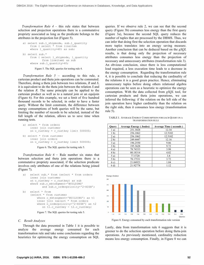
Transformation Rule 4 – this rule states that between selection and projection operations there is a commutative propriety associated as long as the predicate belongs to the attributes in the projection list (Figure 5).

a) select sub.l_shipmode, sub.l_quantity from ( select * from lineitem where l_quantity>40) as sub;

b) select sub.* from ( select l_shipmode, l_quantity from lineitem) as sub where sub.l_quantity>40;


Transformation Rule 5 – according to this rule, a cartesian product and theta join operations can be commuted. Therefore, doing a theta join between two relations, R and S, it is equivalent to do the theta join between the relation S and the relation R. The same principle can be applied to the cartesian product as well as to a natural join or an equijoin (Figure 6). For this example, we set a limit of five hundred thousand records to be selected, in order to have a faster query. Without the limit constraint, the difference between energy consumptions of both queries will be the same, but limiting the number of records to be selected, instead of the full length of the relation, allows us to save time when running tests.

a) select * from orders inner join customer on o_custkey = c_custkey limit 500000;

b) select * from customer inner join orders on o_custkey = c_custkey limit 500000;


Transformation Rule 6 – Rule number six states that between selection and theta join operations there is a commutative propriety associated, if the selection predicate involves only attributes of one of the relations being joined (Figure 7).

a) select sub.* from (select * from orders inner join customer on o_custkey = c_custkey) as sub where sub.c_mktsegment='BUILDING' and sub.o_orderpriority='2-HIGH';

b) select * from (select * from customer where c_mktsegment='BUILDING') as t1 inner join (select * from orders where o_orderpriority='2-HIGH') as t2 on t1.c_custkey = t2.o_custkey;


C. Result Analyzes Through the data presented in Table 1 it is possible to

analyze the average energy consumed for each transformation rule and take some conclusions regarding the heuristics for optimizing the energy consumption on SQL

queries. If we observe rule 2, we can see that the second query (Figure 3b) consumes less energy than the first query (Figure 3a), because the second SQL query reduces the number of tuples that are processed by the DBMS. Thus, we can infer that doing first the selection operation that discards more tuples translates into an energy saving measure. Another conclusion that can be deduced based on the gSQL results, is that doing only the projection of necessary attributes consumes less energy than the projection of necessary and unnecessary attributes (transformation rule 3). An obvious conclusion, since there is less computational load required, a less execution time leads to a decrease in the energy consumption. Regarding the transformation rule 4, it is possible to conclude that reducing the cardinality of the relations it is a good green practice. Hence, eliminating unnecessary tuples before doing others relational algebra operations can be seen as a heuristic to optimize the energy consumption. With the data collected from gSQL tool, for cartesian products and theta joins operations, we can inferred the following: if the relation on the left side of the join operation have higher cardinality than the relation on the right side, then it consumes less energy (transformation rule 5).

TABLE I. AVERAGE ENERGY COMSUMPTION FOR EACH QUERY IN A TRANSFORMATION RULE

Query Average Energy ( Joules) Average Time ( seconds ) 1 a) 251.3028 12.34 1 b) 256.1062 12.5102 2 a) 256.1062 12.5102 2 b) 249.4447 12.16 3 a) 196.2550 9.86 3 b) 195.3628 9.72 4 a) 78.74333 3.98 4 b) 80.18314 4.02 5 a) 77.5720 3.8 5 b) 78.17531 3.72 6 c) 21.04923 1.04 6 d) 21.92778 1.12

Queries

Energy (Joules)

Figure 8. Energy consumed by each transformation rule version

Lastly, data from transformation rule 6 suggests that it is greener to do the selection operation before doing theta-join operations. As previously mentioned, cardinality reduction means less energy consumption. Finally, in Figure 8 we can



63 / 107

see a chart showing the energy consumption of each one of the queries that were used and tested in each transformation rule.

IV. CONCLUSIONS AND FUTURE WORK In this paper, we presented some heuristics to optimize

the energy consumption of relational database queries. The heuristics presented here were devised by analyzing the data from gSQL tool. This was a first approach towards the creation of a more refined set of energy consumption heuristics. As far as we know, nothing similar was done yet in this field of expertise. Saving energy on a query that is executed several times in a data center reduces the monthly energy bill and therefore, decreases the costs of a data center. It is interesting to notice different energy consumptions by doing simple tweaks and transformation rules. Although, we present some heuristics in this paper, some of them having a parallel that corresponds to performance optimization heuristics well defined in the area database systems. Hence, for systems with the same type of hardware optimizing a query to be greener is equivalent to optimizing a query to be faster.

In a near future, we intend to verify if the heuristics proposed here can be transposed to different DBMS. It is important to know how to rank the different DBMS, in order to offer to database administrators the possibility to adopt an eco-friendlier DBMS to support their operational systems. Another issue that we expect to explore is the impact of the established heuristics in DBMS performance structures, such as indexes, execution plans or materialized views, in order to prepare DBMS internal configuration structures regarding energy saving issues.

REFERENCES [1] G. Graefe, “Database servers tailored to improve energy

efficiency,” in Proceedings of the 2008 EDBT Workshop on Software Engineering for Tailor-made Data Management, 2008, pp. 24-28.

[2] M. Jarke, “Query optimization in database systems,” in ACM Computing Surveys, Vol. 16, No. 2, 1984, pp 11-152.

[3] S. Chaudhuri, “An Overview of Query Optimization”. In Proceedings of the seventeenth ACM SIGACT, 1998, pp. 34-43.

[4] S. Ceri and G. Gottlob, “Translating SQL Into Relational Algebra: Optimization, Semantics, and Equivalence of SQL Queries,” in IEEE Transactions on Software Engineering, Vol. SE-11, No. 4, 1985, pp. 324-345.

[5] D. Taniar, H. Khaw, T. H. Cokrowijoyo, and E. Pardede, “The use of Hints in SQL-Nested query optimization,” Information Sciences, Vol. 177, No 12, 2007, pp. 2493-2521.

[6] D. Li, L. Han, and Y. Ding, “YiSQL Query Optimization Methods of Relational Database System,” in Second International Conference on Computer Engineering and Applications, 2010, pp. 557-560.

[7] S. Mittal, “Power Management Techniques for Data Centers: A Survey”, 2014. [online] Available at: http://arxiv.org/abs/1404.6681 [Accessed 11 March 2016].

[8] M. Poess and R. O. Nambiar, “Energy cost, the key challenge of today's data centers: a power consumption analysis of TPC-

C results,” in Proceedings of the VLDB Endowment, vol. 1, 2008, pp. 1229-1240.

[9] R. Gonçalves, J. Saraiva, and O. Belo, “Defining Energy Consumption Plans for Data Querying Processes”. In Proceedings of 2014 IEEE Fourth International Conference on Big Data and Cloud Computing (BdCloud 2014), IEEE computer Society, Sidney, Australia, 2014, pp. 641-647.

[10] T. Carção, “Measuring and visualizing energy consumption within software code”. In: Visual Languages and Human-Centric Computing (VL/HCC), 2014 IEEE Symposium on, July, 2014, pp. 181– 182.

[11] M. Couto, T. Carção, J. Cunha, J. P. Fernandes, and J. Saraiva, “Detecting anomalous energy consumption in android applications”. In Pereira, F.M.Q., ed.: Programming Languages - 18th Brazilian Symposium, SBLP 2014, Maceio, Brazil, October 2-3, 2014. Proceedings. Volume 8771 of Lecture Notes in Computer Science., Springer, 2014, pp. 77–91.

[12] R. Agrawal et al., “The claremont report on database research”. SIGMOD Rec. 37(3), September, 2008, pp. 9–19.

[13] J. Wang, L. Feng, W. Xue, and Z. Song, “A Survey on Energy-efficient Data Management,” in SIGMOD Rec. 40, 2, September, 2011, pp. 17-23.

[14] W. Lang, R. Kandhan, and J. M. Patel, “Rethinking query processing for energy efficiency: Slowing down to win the race”. IEEE Data Eng. Bull. 34(1), 2011, pp. 12–23.

[15] W. Lang and J. M. Patel, “Towards eco-friendly database management systems”. In CIDR 2009, Fourth Biennial Conference on Innovative Data Systems Research, Asilomar, CA, USA, January 4-7, 2009, Online Proceedings, www.cidrdb.org, 2009.

[16] Z. Xu, Y. Tu, and X. Wang, “Exploring power-performance tradeoffs in database systems”. In Li, F., Moro, M.M., Ghandeharizadeh, S., Haritsa, J.R., Weikum, G., Carey, M.J., Casati, F., Chang, E.Y., Manolescu, I., Mehrotra, S., Dayal, U., Tsotras, V.J., eds.: Proceedings of the 26th International Conference on Data Engineering, ICDE 2010, March 1-6, 2010, Long Beach, California, USA, IEEE, 2010, pp. 485–496.

[17] M. Kunjir, P. K. Birwa, and J. R. Haritsa, “Peak power plays in database engines”. In E. A. Rundensteiner, V. Markl, I. Manolescu, S. Amer-Yahia, F. Naumann, and I. Ari, eds.: 15th International Conference on Extending Database Technology, EDBT ’12, Berlin, Germany, March 27-30, 2012, Proceedings, ACM, 2012, pp. 444–455.

[18] M. Rodríguez et al., “Analyzing power and energy consumption of large join queries in database systems,” Industrial Electronics and Applications (ISIEA), 2013 IEEE Symposium on, Kuching, 2013, pp. 148-153.

[19] Z. Xu, Y. Tu, and X. Wang. “PET: reducing Database Energy Cost via Query Optimization,” in Proc. VLDB Endow. 5, 12, August, 2012, pp. 1954-1957.

[20] K. Liu, G. Pinto, and D. Liu, “Data-oriented characterization of application-level energy optimization”, in: Proceedings of the 18th International Conference on Fundamental Approaches to Software Engineering, FASE’15, 2015.

[21] T. Connoly and C. Begg, “Database Systems: A pratical Approach to Design, Implementation, and Management”, 2005, Addison-Wesley Longman Publishing Co., Inc., Boston, USA

[22] A. V. Aho and J. D. Ullman, “Universality of Data Retrieval Languages”, in Proceedings of the 6th ACM SIGACT-SIGPLAN Symposium on Principles of Programming Languages, POPL ’79, (New York, NY, USA), ACM, 1979, pp. 110–119.



64 / 107

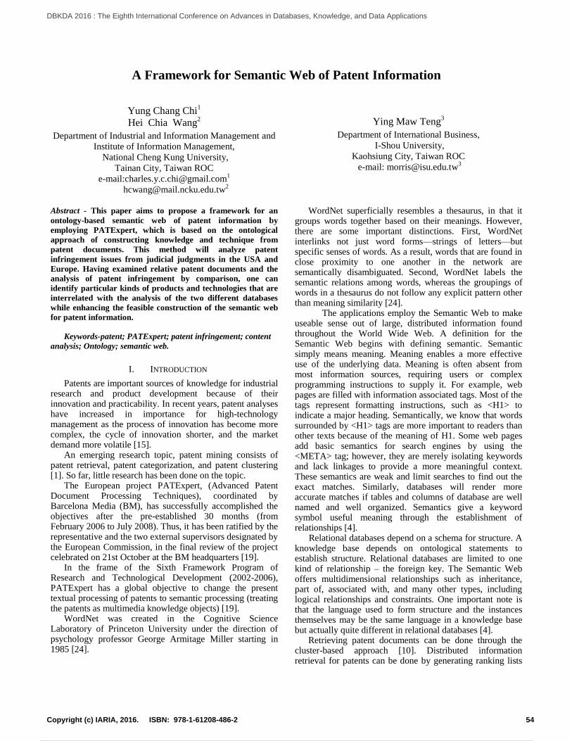
A Framework for Semantic Web of Patent Information

Yung Chang Chi1

Hei Chia Wang2

Department of Industrial and Information Management and

Institute of Information Management,

National Cheng Kung University,

Tainan City, Taiwan ROC

e-mail:[email protected]

[email protected]

Ying Maw Teng3

Department of International Business,

I-Shou University,

Kaohsiung City, Taiwan ROC


Abstract - This paper aims to propose a framework for an

ontology-based semantic web of patent information by

employing PATExpert, which is based on the ontological

approach of constructing knowledge and technique from

patent documents. This method will analyze patent

infringement issues from judicial judgments in the USA and

Europe. Having examined relative patent documents and the

analysis of patent infringement by comparison, one can

identify particular kinds of products and technologies that are

interrelated with the analysis of the two different databases

while enhancing the feasible construction of the semantic web

for patent information.

Keywords-patent; PATExpert; patent infringement; content

analysis; Ontology; semantic web.

I. INTRODUCTION

Patents are important sources of knowledge for industrial research and product development because of their innovation and practicability. In recent years, patent analyses have increased in importance for high-technology management as the process of innovation has become more complex, the cycle of innovation shorter, and the market demand more volatile [15].

An emerging research topic, patent mining consists of patent retrieval, patent categorization, and patent clustering [1]. So far, little research has been done on the topic.

The European project PATExpert, (Advanced Patent Document Processing Techniques), coordinated by Barcelona Media (BM), has successfully accomplished the objectives after the pre-established 30 months (from February 2006 to July 2008). Thus, it has been ratified by the representative and the two external supervisors designated by the European Commission, in the final review of the project celebrated on 21st October at the BM headquarters [19].

In the frame of the Sixth Framework Program of Research and Technological Development (2002-2006), PATExpert has a global objective to change the present textual processing of patents to semantic processing (treating the patents as multimedia knowledge objects) [19].

WordNet was created in the Cognitive Science Laboratory of Princeton University under the direction of psychology professor George Armitage Miller starting in 1985 [24].

WordNet superficially resembles a thesaurus, in that it groups words together based on their meanings. However, there are some important distinctions. First, WordNet interlinks not just word forms—strings of letters—but specific senses of words. As a result, words that are found in close proximity to one another in the network are semantically disambiguated. Second, WordNet labels the semantic relations among words, whereas the groupings of words in a thesaurus do not follow any explicit pattern other than meaning similarity [24].

The applications employ the Semantic Web to make useable sense out of large, distributed information found throughout the World Wide Web. A definition for the Semantic Web begins with defining semantic. Semantic simply means meaning. Meaning enables a more effective use of the underlying data. Meaning is often absent from most information sources, requiring users or complex programming instructions to supply it. For example, web pages are filled with information associated tags. Most of the tags represent formatting instructions, such as <H1> to indicate a major heading. Semantically, we know that words surrounded by <H1> tags are more important to readers than other texts because of the meaning of H1. Some web pages add basic semantics for search engines by using the <META> tag; however, they are merely isolating keywords and lack linkages to provide a more meaningful context. These semantics are weak and limit searches to find out the exact matches. Similarly, databases will render more accurate matches if tables and columns of database are well named and well organized. Semantics give a keyword symbol useful meaning through the establishment of relationships [4]. Relational databases depend on a schema for structure. A knowledge base depends on ontological statements to establish structure. Relational databases are limited to one kind of relationship – the foreign key. The Semantic Web offers multidimensional relationships such as inheritance, part of, associated with, and many other types, including logical relationships and constraints. One important note is that the language used to form structure and the instances themselves may be the same language in a knowledge base but actually quite different in relational databases [4].

Retrieving patent documents can be done through the cluster-based approach [10]. Distributed information retrieval for patents can be done by generating ranking lists



65 / 107

for the query by CORI (The collection retrieval inference network) or KL (Kernighan–Lin) algorithms [13]. Categorizing patent documents can be done automatically by using the k-Nearest Neighbor classifiers and Bayesian classifiers [12][14], or a variety of machine learning algorithms [2], the k-Nearest Neighbor on the basis of patent’s semantic structure [6], or the classifier built through back-propagation network [23]. Clustering algorithms can also be adopted to form a topic map for presenting patent analysis and summarization results [23], and to create a system interface for retrieving patent documents [5].

Content analysis is indigenous to communication research and is potentially one of the most important research techniques in social sciences. It seeks to analyze data within a specific context in view of the meaning someone – a group or a culture – attributes to them. Communications, messages, and symbols differ from observable events, things, properties, or people in that they inform about something other than themselves; they reveal some properties of their distant producers or carriers, and they have cognitive consequences for their senders, their receivers, and the institutions in which their exchange is embedded [7].

Content analysis is a research technique for making replicable and valid inferences from texts to the contexts of their use. As a technique, content analysis involves specialized procedures. It provides new insight, increases a researcher’s understanding of particular phenomena, or informs practical actions. Content analysis is a scientific tool [8].

The judgements of patent infringement, unlike the patent documents, can be mined by using text mining techniques, since the judgments are legal documents. The judgments can be transformed into patterns by content analysis, and readers can easily access them the same way as reading newspapers to understand the key points and issues in dispute.

This study proposes to enhance a semantic web of patent information and patent infringement framework, and the rest of the paper is structured as follows. Section II presents the research background and states the objective. In Section III, we describe our proposed research method. The paper concludes with expected results and future work considerations.

II. RESEARCH BACKGROUND AND OBJECTIVE

So far, patent analysis technologies include patent bibliometric data analysis [3], patent citation analysis [16], patent statistical analysis [22], and patent classification. Patent mining consists of patent retrieval, patent categorization and patent clustering [22]. However, patent infringement constitutes the biggest threat in patent use.

This framework proposes that through patent document mining and judgements of patent infringement analysis, one can discover newly developed products and their similarity with the claims of other patents, and foresee where potential patent threats are and the likelihood of patent infringement. While constructing the patent Semantic Web, the ontology and rules engines must include it.

This framework of patent database is based on the databases of United States Patent and Trademark Office (USPTO) and the European Patent Office (EPO). The patent infringement judgements are based on the judicial judgments in United States and European Union.

The purposes of this study is to construct the Semantic Web of patent information, and reference regarding patent infringement, technology trends for new product designers and technology research engineers at the stage before and after developing a new product or technology. With the analyzed information, managerial team can make sound strategic decisions.

It is difficult for laymen or ordinary readers who are short of legal background to fully grasp the gist of judicial judgments rendered by judges. With the implementation of content analysis and the big data concept, ordinary people can use content analysis technology to analyze patent infringements with the help of a semantic web.

III. RESEARCH METHOD

Patent documents can be collected from United States

Patent and Trademark Office (USPTO) patent database and

the European Patent Office (EPO) patent database. The

patent infringement content can be collected from the “West

Law” database.

A. Patent documents analysis

Based on the collected patent documents and the subject-action-object (SAO) structures extracted by using Natural Language Processing (NLP), the study uses a content analysis approach to generate the concepts and relationships of related patent documents.

NLP is a text mining technique that can conduct syntactic analysis of natural language; NLP tools include the Stanford parser (Stanford 2013) [21], Minipar (Lin 2003) [17], and Knowledgist TM2.5 [11].

NLP tools will be used for building a set of SAO structures from the collected patents.

Multidimensional scaling (MDS) is a statistical technique used to visualize similarities in data [9][20]. Patent documents in different fields have different key issues that trigger different multidimensional scaling, so the paper will design a new algorithm to identify which particular patent field shall correspond to what extent of scaling.

The analysis patent documents for specified keywords and returns a list of the documents where the keywords were found. Then, the framework will use data and text mining technology to design a specified algorithm (still in progress) in order to analyze the legal documents and try to find out the most similar patents or patent group.

B. Patent infringement content analysis

The most obvious source of data appropriate for content analysis is the text to which meanings are conventionally attributed: verbal discourse, written documents, and visual representations. The text in the patent infringement judgements is important because that is where the meanings are. For this reason, it is essential for the content analysis technology to analyze the patent infringement text in order to



66 / 107

develop strategies and preventive measures in patent litigation.

The judgements of patent infringement, unlike the patent documents, can be mined using text mining techniques, since the judgements are legal documents. The judgements can be transformed into patterns by content analysis, and readers can easily access them the same way as reading newspapers to understand the key points and issues in dispute.

Content analyses commonly contain six steps that define the technique procedurally, as follows:

Design. Design is a conceptual phase during which analysts (i) define their context, what they wish to know and are unable to observe directly; (ii)explore the source of relevant data that either are or may become available; and (iii)adopt an analytical construct that formalizes the knowledge available about the data-context relationship thereby justifying the inferential step involved in going from one to the other.

Unitizing. Unitizing is the phase of defining and ultimately identifying units of analysis in the volume of available data. Sampling units make possible the drawing of a statistically representative sample from a population of potentially available data, such as issues of a newspaper, whole books, television episodes, fictional characters, essays, advertisements.

Sampling. While the process of drawing representative samples is not indigenous to content analysis, there is the need to (1) undo the statistical biases inherent in much of the symbolic material analyzed and (2) ensure that the often conditional hierarchy of chosen sampling units become representative of the organization of the symbolic phenomena under investigation.

Coding. Coding is the step of describing the recording units or classifying them in terms of the categories of the analytical constructs chosen. This step replicates an elementary notion of meaning and can be accomplished either by explicit instructions to trained human coders or by computer coding. The two evaluative criteria, reliability as measured by inter coder agreement and relevance or meaningfulness, are often at odds.

Drawing inferences. Drawing inferences is the most important phase in a content analysis. It applies the stable knowledge about how the variable accounts of coded data are related to the phenomena the researcher wants to know about.

Validation. Validation is the desideratum of any research effort. However, validation of content analysis results is limited by the intention of the technique to infer what cannot be observed directly and for which validation evidence is not readily available.

The patent infringement content analysis searches the patent infringement judgements for specific keywords and returns a list of the documents as above patent documents by introducing the content analysis technology into specified design algorithm (still in progress) in order to analyze the infringement cases/precedents. It also finds the nearest infringement judgements/precedents.

C. Constructing Semantic Web

Our proposed semantic web, which has a structure based

on Figure 4, is a program that has the following parts:

(1) The first part searches patent documents for specified

keywords and returns a list of the documents where the

keywords were found. Then, the program will use data and

text mining technology to design a specified algorithm in

order to analyze the legal documents and try to find out the

most similar patents or patent group concepts and

relationships. The results from part (1) constructing the

knowledge repository for the Reasoners are shown in Figure

1.

(2) Next, it searches the patent infringement judgments

for specific keywords and returns a list of the documents as

above patent documents by introducing the content analysis

technology into a specified design algorithm in order to

analyze the infringement cases/precedents. It also finds the

nearest infringement judgements/precedents and description

logic. The results from part (2) constructing the knowledge

repository for the Rules engines are shown in Figure 3.

(3) Reasoners: Reasoners add inference to the Semantic

Web. Inference creates logical additions that offer

classification and realization. Classification populates the

class structure, allowing concepts and relationships to relate

properly to others, such as a person is a living thing, father

is a parent, married is a type of relationship, or married is a

symmetric relationship. Realization offers the same, for

example, John H is the same as JH, for instance. There are

several types of reasoners offering various levels of

reasoning. Reasoners often plug in other tools and

frameworks. Reasoners leverage asserted statements to

create logically valid ancillary statements [4].

(4)The semantic web components of Rules engines

support inference typically beyond what can be deduced

from description logic. The engines add a powerful

dimension to the knowledge constructs. Rules enable the

merging of ontologies and other larger logical tasks,

including programming methods such as count and string

searches [4].

So far, the whole approach is purely theoretical at the

moment. But in the patent document analysis, we have

successful employed WordNet by the word similarity matrix

clustering of words and merged with the similar semantic

terms from a lower term dimensional approach. In the

related data-mining fields, the semantic web system as

WordNet can be employed to identify keywords, connect

similar words, features, and sparse matrix to prevent the

miscarriage of patent retrievals, waste of time and risks of

patent infringement as well. The WordNet can also save

storage memory while advancing the accuracy of text-

mining in regards to ordinary, literal, and professional

meaning of keywords and promoting the retrieval speed of

patent research.



67 / 107

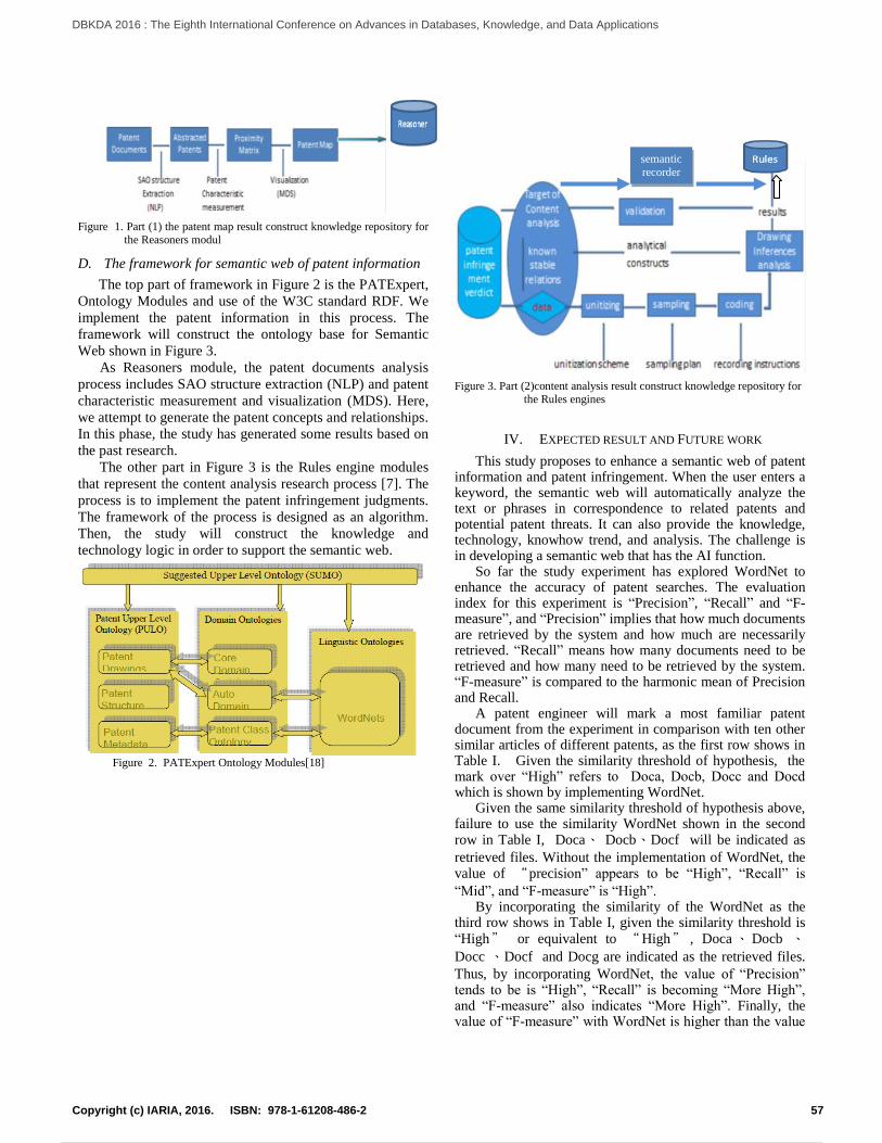
Figure 1. Part (1) the patent map result construct knowledge repository for the Reasoners modul

D. The framework for semantic web of patent information

The top part of framework in Figure 2 is the PATExpert,

Ontology Modules and use of the W3C standard RDF. We

implement the patent information in this process. The

framework will construct the ontology base for Semantic

Web shown in Figure 3.

As Reasoners module, the patent documents analysis

process includes SAO structure extraction (NLP) and patent

characteristic measurement and visualization (MDS). Here,

we attempt to generate the patent concepts and relationships.

In this phase, the study has generated some results based on

the past research.

The other part in Figure 3 is the Rules engine modules

that represent the content analysis research process [7]. The

process is to implement the patent infringement judgments.

The framework of the process is designed as an algorithm.

Then, the study will construct the knowledge and

technology logic in order to support the semantic web.

Figure 2. PATExpert Ontology Modules[18]

Figure 3. Part (2)content analysis result construct knowledge repository for the Rules engines

IV. EXPECTED RESULT AND FUTURE WORK

This study proposes to enhance a semantic web of patent information and patent infringement. When the user enters a keyword, the semantic web will automatically analyze the text or phrases in correspondence to related patents and potential patent threats. It can also provide the knowledge, technology, knowhow trend, and analysis. The challenge is in developing a semantic web that has the AI function.

So far the study experiment has explored WordNet to enhance the accuracy of patent searches. The evaluation index for this experiment is “Precision”, “Recall” and “F-measure”, and “Precision” implies that how much documents are retrieved by the system and how much are necessarily retrieved. “Recall” means how many documents need to be retrieved and how many need to be retrieved by the system. “F-measure” is compared to the harmonic mean of Precision and Recall.

A patent engineer will mark a most familiar patent document from the experiment in comparison with ten other similar articles of different patents, as the first row shows in Table I. Given the similarity threshold of hypothesis, the mark over “High” refers to Doca, Docb, Docc and Docd which is shown by implementing WordNet.

Given the same similarity threshold of hypothesis above, failure to use the similarity WordNet shown in the second row in Table I, Doca、 Docb、Docf will be indicated as

retrieved files. Without the implementation of WordNet, the value of “precision” appears to be “High”, “Recall” is

“Mid”, and “F-measure” is “High”. By incorporating the similarity of the WordNet as the

third row shows in Table I, given the similarity threshold is “High” or equivalent to “High” , Doca、Docb 、Docc 、Docf and Docg are indicated as the retrieved files.

Thus, by incorporating WordNet, the value of “Precision” tends to be is “High”, “Recall” is becoming “More High”, and “F-measure” also indicates “More High”. Finally, the value of “F-measure” with WordNet is higher than the value

semantic

recorder



68 / 107

of “F-measure” without WordNet. Thus, the integration of WordNet is more likely to generate more precise meanings for patent searches.

The finding of the experiment is that WordNet can generate more wording accuracy of text-mining as to ordinary, literal and professional meanings of keywords, while promoting the retrieval speed of patent research and mitigating waste of time.

TABLE I. WORDNET SIMILARITY COMPARISON TABLE

The study difficulties are in employing different analysis

methods to analyze different databases and further, integrating these analysis results with the semantic web. An accurate algorithm in different fields must be constructed and achieved with the semantic web.

The obstacles are in integrating much more research math and different databases. Results need to be standardized and communicated, compared, and exchanged with each other.

Furthermore, the study aims to employ different analysis methods to analyze various databases with the analysis results in Semantic Web. An accurate algorithm in different fields can be feasibly constructed and achieved in the analysis of patent information and patent infringement.

The next steps will be to employ the Semantic Web impacts functions to increase the new data automatically. Figure 4 indicates major Semantic Web components: the right side is Rules engine, the left side is the Reasoner, over the center side is base ontology from the PATExpert ontology modules, and under the center side is language. The next steps of Semantic Web will be developed to use different languages, construct a multi-language Semantic Web, in order to retrieve from different country’s patent databases.

Figure 4. Major Semantic Web components [4]

The Semantic Web can employ the image recognition

functions to identify drawings and pictures. If the Semantic Web has the capability of analyzing drawings and pictures, the accuracy of the results will be increased in the future.

References

[1] Y. L. Chen, and Y. T. Chiu, “An IPC-based vector space model for patent retrieval” Information Processing and Management, pp.309-322.47, 2011.

[2] C. J. Fall, A. Torcsrari, K. Benzineb, and G. Karetka, “SIGIR Forum” Automated categorization in the international patent classification, pp.10-25. 37(1), 2003.

[3] V. K. Gupta, and N. B. Pangannaya, Carbon nanotubes; “Bibliometric analysis of patents”, World Patent Information, pp.185-189.Vol.22,issue 3, Sep. 2000.

[4] J. Hebeler, M. Fisher, R. Blace and A. Perez-Lopez, “Semantic Web Programming “Wiley Publishing, Inc.2009.

[5] S. H. Huang, C. C. Liu, C. W. Wang, H. R. Ke, and W. P. Yang, “International Computer Symposium” Knowledge annotation and discovery for patent analysis, pp.15-20, 2004.

[6] J.H. Kim, and K.S. Choi, Patent document categorization based on semantic structural information, “Information processing & Management”, pp.1200-1215.43(5), 2007.

[7] K. Krippendorff, Content analysis In E. Barnouw, G. Gerbner, W. Schramm, T. L. Worth, and L. Gross (Eds.), International encyclopedia of communication New York, NY: Oxford University Press, pp.403-407.Vol. 1, 1989.

[8] K. Krippendorff, “Content Analysis An Introduction to Its Methodology” second Edition, Sage Publications, Inc. 2004.

[9] J. B. Kruskal, Multidimensional scaling by optimizing goodness of fit to a nonmetric hypothesis. Psychometrika, pp.1-27.29(1), 1964.

[10] I. S. Kang, S. H. Na, J. Kim, and J. H. Lee, “Information Processing & Management”Cluster-based patent retrieval, pp.1173-1182.43(5), 2007.

[11] Knowledgist retrieves, analyzes, and organizes information. https://invention-machine.com/ , retrieved: Apr., 2016

[12] L. S Larkey., Some issues in the automatic classification of U.S. patents. In: Working notes for the AAAI-98 workshop on learning for text categorization, pp.87-90, 1998.

[13] L. S. Larkey, Connell, M. E., and Callan, J. Collection selection and results merging with topically organized US patents and TREC data.

Patent Engineer marked similarity

No include WordNet income of similarity

Include WordNet income of similarity

Similarity(Docx,Doca) Most High High More High

Similarity(Docx,Docb) More High More High More High

Similarity(Docx,Docc) More High Mid High

Similarity(Docx,Docd) High Low Mid

Similarity(Docx,Doce) Mid Low Mid

Similarity(Docx,Docf) Low High More High

Similarity(Docx,Docg) More Low Mid High

Similarity(Docx,Doch) More Low Low Mid

Similarity(Docx,Doci) Most Low Most Low More Low

Similarity(Docx,Docj) None Most Low More Low



69 / 107

In Proceedings of ninth international conference on informaiton knowledge and management, pp.282-289, 2000.

[14] L. S. Larkey, A patent search and classification system. In: Proceedings of the fourth ACM conference on digital libraries, pp.79-87, 1999.

[15] Y. Liang, R. Tan, and J. Ma, “Patent Analysis with Text Mining for TRIZ” IEEE ICMIT, pp.1147-1151, 2008.

[16] J. Michel, and B. Bettels, “Patent citation analysis: a closer look at the basic input data from patent search reports”, Scientometrics, pp.185-201. Vol.51. no. 1, 2001.

[17] MINIPAR http://webdocs.cs.ualberta.ca/~lindek/minipar.htm , retrieved:Dec., 2015

[18] PATExpert http://cordis.europa.eu/ist/kct/patexpert_synopsis.htm , retrieved: Feb., 2016

[19] PATExpet http://www.barcelonamedia.org/report/the-european-project-patexpert-coordinated-by-bm-finishes-with-fulfilled-objectives-and-success , retrieved: Feb., 2016

[20] U. Schmoch, “International Journal of Technology Management” Evaluation of technological strategies of companies by means of MDS maps., pp.4-5.10(4-5), 1995.

[21] The Stanford Natural Language Processing Group, The Stanford Parser: A statistical parser, http://nlp.stanford.edu/software/lex-parser.shtml

[22] Y. H. Tseng, C. J. Lin, and Y. I. Lin, “Text mining for patent mapanalysis”, Information Processing & Mangement, pp.1216-1247. vol.43, issue 5, Sep. 2007.

[23] A. J.C. Trappey, F. C. Hsu, C V. Trappy,and C. I. Lin,” Development of a patent document classification and search platform using a back-propagation network”, Expert Systems with Applications, pp.755-765.31(4), 2006.

[24] WordNet https://wordnet.princeton.edu/, retrieved: May, 2016



70 / 107

A Comparison of Two MLEM2 Rule Induction AlgorithmsApplied to Data with Many Missing Attribute Values

Patrick G. Clark and Cheng Gao

Department of Electrical Engineeringand Computer Science,

University of KansasLawrence, KS, USA

Email: [email protected]@ku.edu

Jerzy W. Grzymala-Busse

Department of Electrical Engineeringand Computer Science,University of Kansas,Lawrence, KS, USA

Department of Expert Systemsand Artificial Intelligence,University of Information

Technology and Management,Rzeszow, Poland

Email: [email protected]

Abstract—We present results of novel experiments, conducted on18 data sets with many missing attribute values, interpreted aslost values, attribute-concept values and “do not care” conditions.The main objective was to compare two versions of the ModifiedLearning from Examples, version 2 (MLEM2) rule inductionalgorithm, emulated and true, using concept probabilistic ap-proximations. Our secondary objective was to check which inter-pretation of missing attribute values provides the smallest errorrate, computed as a result of ten-fold cross validation. Resultsof our experiments show that both versions of the MLEM2 ruleinduction algorithms do not differ much. On the other hand,there is some evidence that the lost value interpretation of missingattribute values is the best: in seven cases this interpretation wassignificantly better (with 5% of significance level, two-tailed test)than attribute-concept values, and in eight cases it was better than“do not care” conditions. Additionally, attribute-concept valuesand “do not care” conditions were never significantly better thanlost values.

Keywords–Probabilistic approximations; generalization of prob-abilistic approximations; concept probabilistic approximations; trueMLEM2 algorithm; emulated MLEM2 algorithm.

I. INTRODUCTION

Lower and upper approximations are basic ideas of roughset theory. Probabilistic approximations, associated with aprobability α, are a generalization of that idea. If α = 1,the probabilistic approximation is identical with the lowerapproximation, if α is a very small positive number, theprobabilistic approximation is identical with the upper approx-imation. Probabilistic approximations, for completely specifieddata sets, were studied, e.g., in [1]–[9]. Probabilistic approxi-mations were additionally generalized to describe incompletedata sets in [10]. Experimental research associated with suchprobabilistic approximations was initiated in [11][12].

In this paper, missing attribute values are interpreted as lostvalues, attribute-concept values, and “do not care” conditions.A lost value is denoted by “?”, an attribute-concept value isdenoted by “−”, and a “do not care” condition is denoted by“*”. With lost values we assume that the original attribute valuewas erased, and that we should induce rules from existing,specified attribute values. With attribute-concept value we

assume that such missing attribute values may be replaced byany actual attribute value restricted to the concept to which thecase belongs. For example, if our concept is a specific disease,an attribute is a diastolic pressure, and all patients affected bythe disease have high or very high diastolic pressure, a missingattribute value of the diastolic pressure for a sick patient willbe high or very-high. With the third interpretation of missingattribute values, the “do not care” condition, we assume thatit does not matter what is the attribute value. Such value maybe replaced by any value from the set of all possible attributevalues.

For any concept X and probability α, its probabilisticapproximations may be computed directly from correspondingdefinitions and implemented as a new program. The output ofthis program may be used as an input to an implementation ofthe MLEM2 algorithm. The respective MLEM2 rule inductionalgorithm will be called a true MLEM2 algorithm.

Another possibility is to use the existing data mining sys-tem Learning from Examples using Rough Set theory (LERS).LERS computes standard lower and upper approximations forany concept. In LERS there exists a component that imple-ments the MLEM2 rule induction algorithm. This componentmay be used to compute possible rules from the probabilisticapproximation of X . Some modification of the strength ofinduced rules is required. This approach will be called anemulated MLEM2 algorithm. It is easier to implement sinceall what we need to do is to compute the probabilistic ap-proximation of X and to modify strengths. The main part,the MLEM2 rule induction algorithm, does not need to beseparately implemented. The idea of the emulated MLEM2algorithm was introduced in [13] and further developed in[14][15].

Experiments conducted on eight incomplete data sets with35% of missing attribute values to compare true version ofthe MLEM2 rule induction algorithm with the emulated onewere reported in [16]. All three interpretations of missingattribute values were used in experiments, so experiments wereconducted on 24 data sets. In these experiments true andemulated versions of the MLEM2 algorithm were compared



71 / 107

using the resulting classification error rate of the induced rulesagainst the ten-fold cross validated data set as the qualitycriterion. Results were inconclusive. For six data sets, for allvalues of the parameter α, results were identical; for other14 data sets results did not differ significantly (we used theWilcoxon matched-pairs signed rank test, 5% significancelevel, two-tailed test). For three other data sets, the trueMLEM2 algorithm was better than emulated, for remainingone data set the emulated MLEM2 algorithm was better thanthe true one.

Usually, experiments conducted on data sets with manymissing attribute values provide for more conclusive results.As a result our first objective in this paper was to conductnew experiments with data sets that contain more than 35%missing attribute values. We used three interpretations ofmissing attribute values, resulting in 18 combinations. Resultsof the same comparison of error rate of the induced rules aremeasurably more conclusive: in five combinations (out of 18)the emulated approach to MLEM2 algorithm was better, inone case the true approach was better (5% significance level,two-tailed test).

Our second objective was to check which interpretation ofmissing attribute values should be used to accomplish a lowererror rate. There is some evidence that the lost value interpre-tation of missing attribute values is the best: in seven cases thisinterpretation was significantly better (with 5% of significancelevel, two-tailed test) than attribute-concept values, and in eightcases it was better than “do not care” conditions. Additionally,attribute-concept values and “do not care” conditions werenever significantly better than lost values.

In Sections II and III background information on incom-plete data sets and probabilistic approximations is covered.Section IV describes the two algorithms used in our ruleinduction experiments and Section V explains the experimentalsetup with our results. Finally we provide concluding remarksin Section VI.

II. INCOMPLETE DATA SETS

An example of incomplete data set is presented in Table I.In Table I, the set A of all attributes consists of three variablesWind, Humidity and Temperature. A concept is a set of allcases with the same decision value. There are two conceptsin Table I, the first one contains cases 1, 2, 3 and 4 and ischaracterized by the decision value yes of decision Trip. Theother concept contains cases 5, 6, 7 and 8 and is characterizedby the decision value no.

The fact that an attribute a has the value v for the casex will be denoted by a(x) = v. The set of all cases will bedenoted by U . In Table I, U = {1, 2, 3, 4, 5, 6, 7, 8}.

For complete data sets, an attribute-value pair (a, v) = t,a block of t, denoted by [t], is a set of all cases from U suchthat attribute a has a value v. An indiscernibility relation Ron U is defined for all x, y ∈ U by

xRy if and only if a(x) = a(y) for all a ∈ A.

For incomplete decision tables the definition of a block ofan attribute-value pair must be modified in the following way[17][18]:

• If for an attribute a there exists a case x such thata(x) =?, i.e., the corresponding value is lost, then the

TABLE I. AN INCOMPLETE DATA SET

Attributes Decision

Case Wind Humidity Temperature Trip

1 low * low yes2 * low − yes3 high low low yes4 low * * yes5 high high high no6 ? − high no7 low low * no8 high ? low no

case x should not be included in any blocks [(a, v)]for all values v of attribute a,

• If for an attribute a there exists a case x such thatthe corresponding value is an attribute-concept value,i.e., a(x) = −, then the corresponding case x shouldbe included in blocks [(a, v)] for all specified valuesv ∈ V (x, a) of attribute a, where

V (x, a) = {a(y) | a(y) is specified , y ∈ U,d(y) = d(x)}, (1)

and d is the decision.• If for an attribute a there exists a case x such that

the corresponding value is a “do not care” condition,i.e., a(x) = ∗, then the case x should be included inblocks [(a, v)] for all specified values v of attribute a.

For a case x ∈ U the characteristic set KB(x) is definedas the intersection of the sets K(x, a), for all a ∈ B, whereB is a subset of the set A of all attributes and the set K(x, a)is defined in the following way:

• If a(x) is specified, then K(x, a) is the block[(a, a(x))] of attribute a and its value a(x),

• If a(x) =? or a(x) = ∗ then the set K(x, a) = U ,• If a(x) = −, then the corresponding set K(x, a) is

equal to the union of all blocks of attribute-value pairs(a, v), where v ∈ V (x, a) if V (x, a) is nonempty. IfV (x, a) is empty, K(x, a) = U .

The characteristic set KB(x) may be interpreted as the setof cases that are indistinguishable from x using all attributesfrom B and using a given interpretation of missing attributevalues.

For the data set from Table I, the set of blocks of attribute-value pairs is

[(Wind, low)] = {1, 2, 4, 7},[(Wind, high)] = {2, 3, 5, 8},[(Humidity, low)] = {1, 2, 3, 4, 6, 7},[(Humidity, high)] = {1, 4, 5, 6},[(Temperature, low)] = {1, 2, 3, 4, 7, 8},[(Temperature, high)] = {4, 5, 6, 7}.

For Table I, V (2, T emperature) = {low} andV (6, Humidity) = {low, high}.

The corresponding characteristic sets are



72 / 107

TABLE II. CONDITIONAL PROBABILITIES

Case x Characteristic set KA(x) Pr({1, 2, 3, 4} | KA(x))

1 {1, 2, 4, 7} 0.752 {1, 2, 3, 4, 7} 0.83 {2, 3} 14 {1, 2, 4, 7 } 0.755 {5} 06 {4, 5, 6, 7} 0.257 {1, 2, 4, 7} 0.758 {2, 3, 8} 0.667

KA(1) = [(Wind, low)] ∩ [(Humidity, ∗)] ∩ [(Temp, low)]

= {1, 2, 4, 7} ∩ U ∩ {1, 2, 3, 4, 7, 8}= {1, 2, 4, 7},

KA(2) = {1, 2, 3, 4, 7},KA(3) = {2, 3},KA(4) = {1, 2, 4, 7},KA(5) = {5},KA(6) = {4, 5, 6, 7},KA(7) = {1, 2, 4, 7},KA(8) = {2, 3, 8}.

III. PROBABILISTIC APPROXIMATIONS

For incomplete data sets there exist a number of differentdefinitions of approximations, in this paper we will use onlyconcept approximations, we will skip the word concept.

The B-lower approximation of X , denoted by appr(X), isdefined as follows

∪ {KB(x) | x ∈ X,KB(x) ⊆ X}. (2)

Such lower approximations were introduced in [17][19].The B-upper approximation of X , denoted by appr(X), is

defined as follows

∪ {KB(x) | x ∈ X,KB(x) ∩X 6= ∅}= ∪ {KB(x) | x ∈ X}.

(3)

These approximations were studied in [17][19][20].For incomplete data sets there exist a few definitions

of probabilistic approximations, we will use only conceptprobabilistic approximations, again, we will skip the wordconcept.

A B-probabilistic approximation of the set X with thethreshold α, 0 < α ≤ 1, denoted by B-apprα(X), is definedas follows

∪{KB(x) | x ∈ X, Pr(X|KB(x)) ≥ α}, (4)

where Pr(X|KB(x)) =|X∩KB(x)||KB(x)| is the conditional proba-

bility of X given KB(x). A-probabilistic approximations ofX with the threshold α will be denoted by apprα(X).

For Table I and the concept X = [(Trip, yes)] = {1, 2, 3,4}, for any characteristic set KA(x), x ∈ U , all conditionalprobabilities P (X|KA(x)) are presented in Table II.

There are five distinct conditional probabilitiesPr({1, 2, 3, 4} | KA(x)), x ∈ U : 0.25, 0.667, 0.75, 0.8and 1. Therefore, there exist at most five distinct probabilisticapproximations of {1, 2, 3, 4} (in our example, there areonly two distinct probabilistic approximations of {1, 2,3, 4}). A probabilistic approximation apprβ({1, 2, 3, 4}),with β > 0 and not listed below, is equal to the closestprobabilistic approximation apprα({1, 2, 3, 4}) with α largerthan or equal to β. For example, appr0.7({1, 2, 3, 4}) =appr0.8({1, 2, 3, 4}). For Table I, all distinct probabilisticapproximations are

appr0.8({1, 2, 3, 4}) = KB(2) ∪KB(3)

= {1, 2, 3, 4, 7} ∪ {2, 3}= {1, 2, 3, 4, 7},

appr1({1, 2, 3, 4}) = KB(3) = {2, 3},appr0.25({5, 6, 7, 8}) = {1, 2, 3, 4, 5, 6, 7, 8},appr0.333({5, 6, 7, 8}) = {2, 3, 4, 5, 6, 7, 8},appr0.75({5, 6, 7, 8}) = {4, 5, 6, 7},appr1({5, 6, 7, 8}) = {5}.

IV. RULE INDUCTION

In this section we will discuss two different ways to inducerule sets using probabilistic approximations: true MLEM2 andemulated MLEM2.

A. True MLEM2In the true MLEM2 approach, for a given concept X and

parameter α, first we compute the probabilistic approximationapprα(X). The set apprα(X) is a union of characteristic sets,so it is globally definable [21]. Thus, we may use the MLEM2strategy to induce rule sets [22][23] by inducing rules directlyfrom the set apprα(X). For example, for Table I, for theconcept [(Trip, no)] = {5, 6, 7, 8} and for the probabilisticapproximation appr0.75({5, 6, 7, 8}) = {4, 5, 6, 7}, using thetrue MLEM2 approach, the following single rule is induced

1, 3, 4(Temperature, high) -> (Trip, no).

Rules are presented in the LERS format, every rule isassociated with three numbers: the total number of attribute-value pairs on the left-hand side of the rule, the total numberof cases correctly classified by the rule during training, andthe total number of training cases matching the left-hand sideof the rule, i.e., the rule domain size.

B. Emulated MLEM2We will discuss how the existing rough set based data

mining systems, such as LERS, may be used to induce rulesusing probabilistic approximations. All what we need to do,for every concept, is to modify the input data set, run LERS,and then edit the induced rule set [14]. We will illustrate thisprocedure by inducing a rule set for Table I and the concept[(Trip, no)] = {5, 6, 7, 8} using the probabilistic approximationappr0.75({5, 6, 7, 8}) = {4, 5, 6, 7}. First, a new data setshould be created in which for all cases that are members of theset appr0.75({5, 6, 7, 8}) the decision values are copied fromthe original data set (Table I). For all remaining cases, thosenot being in the set appr0.75({5, 6, 7, 8}), a new decision value



73 / 107

TABLE III. A PRELIMINARY MODIFIED DATA SET

Attributes Decision

Case Wind Humidity Temperature Trip

1 low * low SPECIAL2 * low − SPECIAL3 high low low SPECIAL4 low * * yes5 high high high no6 ? − high no7 low low * no8 high ? low SPECIAL

is introduced. In our experiments the new decision value wasnamed SPECIAL. Thus a new data set is created, see Table III.

This data set is input into the LERS data mining system.The concept [(Trip, no)], computed from Table III, is {5, 6,7}. The LERS system computes the concept upper conceptapproximation of the set {5, 6, 7} to be {1, 2, 4, 5, 6, 7},and using this approximation, computes the correspondingfinal modified data set. The MLEM2 algorithm induces thefollowing preliminary rule set from the final modified datasets

1, 4, 6(Temperature, low) -> (Trip, SPECIAL)1, 1, 4(Wind, low) -> (Trip, yes)1, 1, 4(Wind, low) -> (Trip, no)1, 2, 4(Humidity, high) -> (Trip, no)

where the three numbers that precede every rule are computedfrom Table III. Because we are inducing rules for the approx-imation from (Trip, no) ({5, 6, 7}), only the last two rules

1, 1, 4(Wind, low) -> (Trip, no)1, 2, 4(Humidity, high) -> (Trip, no)

should be saved and the remaining two rules should be deletedin computing the final rule set.

In the preliminary rule set, the three numbers that precedeevery rule are adjusted taking into account the preliminarymodified data set. Thus during classification of unseen casesby the LERS classification system rules describe the originalconcept probabilistic approximation of the concept X .

V. EXPERIMENTS

In our experiments, we used six real-life data sets takenfrom the University of California at Irvine Machine LearningRepository, see Table IV. For every data set a set of templateswas created. Templates were formed by replacing incremen-tally (with 5% increment) existing specified attribute values bylost values. Thus, we started each series of experiments withno lost values, then we added 5% of lost values, then we added

25

35

45

55

65

75

85

95

0 0.2 0.4 0.6 0.8 1

Erro

r rat

e (%

)

Parameter alpha

?, true MLEM2 -, true MLEM2 *, true MLEM2 ?, emulated MLEM2 -, emulated MLEM2 *, emulated MLEM2

Figure 1. Breast cancer data set

29

31

33

35

37

39

41

0 0.2 0.4 0.6 0.8 1

Erro

r rat

e (%

)

Parameter alpha


Figure 2. Echocardiogram data set

15

17

19

21

23

25

27

29

0 0.2 0.4 0.6 0.8 1

Erro

r rat

e (%

)

Parameter alpha


Figure 3. Hepatitis data set

additional 5% of lost values, etc., until at least one entire rowof the data sets was full of lost values. Then, three attemptswere made to change the configuration of new lost valuesand either a new data set with extra 5% of lost values wascreated or the process was terminated. Additionally, the same



74 / 107

50

55

60

65

70

75

80

85

90

95

100

0 0.2 0.4 0.6 0.8 1

Erro

r rat

e (%

)

Parameter alpha

?, true MLEM2 ?, emulated MLEM2 -, true MLEM2 -, emulated MLEM2 *, true MLEM2 *, emulated MLEM2

Figure 4. Image segmentation data set

35 40 45 50 55 60 65 70 75 80 85 90 95

100

0 0.2 0.4 0.6 0.8 1

Erro

r rat

e (%

)

Parameter alpha


Figure 5. Lymphography data set

20

30

40

50

60

70

80

90

100

0 0.2 0.4 0.6 0.8 1

Erro

r rat

e (%

)

Parameter alpha


Figure 6. Wine recognition data set

templates were edited for further experiments by replacingquestion marks, representing lost values by “−”s, representingattribute-concept values, and then by “*”s, representing “donot care” conditions.

For any data set, there was some maximum for the percent-age of missing attribute values. For example, for the Breastcancer data set, it was 44.81%. In our experiments we usedonly such incomplete data sets, with as many missing attributevalues as possible. Note that for some data sets the maximumof the number of missing attribute values was less than 40%,we have not used such data for our experiments. Thus, forany data set from Table IV, three data sets were used forexperiments, so the total number of data sets was 18.

Our first objective was to compare both approaches to ruleinduction, true MLEM2 and emulated MLEM2, in terms ofthe classification error rate of the induced rules. Results ofour experiments are presented in Figures 1–6, with lost valuesdenoted by “?”, attribute-concept values denoted by “−”, and“do not care” conditions denoted by “*”.

For five combinations of data set and interpretation ofmissing attribute values the error rate was significantly smallerfor the emulated version of MLEM2. The five combinationsincluded Breast cancer and Image segmentation with “?” and“−”, and Echocardiogram with “?”. For Wine recognition with“−”, the error rate was significantly smaller for the true versionof MLEM2. In the remaining 12 combinations the differencein error rate was not significant (5% significance level, two-tailed test) and for the Breast cancer with “−” combination,the error rate for both versions of the MLEM2 algorithm wasidentical for all 11 values of α.

Our second objective was to check which interpretationof missing attribute value provides the smallest error rate,computed as a result of ten-fold cross validation. In eightcombinations the error rate was significantly smaller for “?”than for “*”. The eight combinations included both true andemulated MLEM2 with the Image segmentation, Lymphogra-phy and Wine recognition data sets, and emulated MLEM2with the Echocardiogram and Hepatitis data sets.

For the following seven combinations the error rate wassignificantly smaller for “?” than for “−”. The seven com-binations included both true and emulated MLEM2 with theBreast cancer and Wine recognition data sets, true MLEM2with Image segmentation and Lymphography, and emulatedMLEM2 with the Echocardiogram data set.

In four combinations the error rate was measurably smallerfor “−” than “?”. The four combinations included both trueand emulated MLEM2 with the Hepatitis data set and emulatedMLEM2 with the Image segmentation and Wine recognitiondata sets.

For one combination the error rate was smaller for “*” thanfor “−”, true MLEM2 and the Breast cancer data set. However,for the remaining combinations the difference in error rate wasnot significant. In addition, “−” and “*” values were neversignificantly better than “?”.

VI. CONCLUSIONS

In our experiments we compared true and emulated ver-sions of the MLEM2 algorithm using the error rate of theinduced rule set, a result of ten-fold cross validation, as thequality criterion. Results of the same comparison of error rateof the induced rules are measurably more conclusive thanprevious experiments: in five combinations (out of 18) theemulated approach to MLEM2 algorithm was better, in one



75 / 107

TABLE IV. DATA SETS USED FOR EXPERIMENTS

Data set Number of % of

cases attributes concepts missing values

Breast cancer 277 9 2 44.81Echocardiogram 74 7 2 40.15Hepatitis 155 19 2 60.27Image segmentation 210 19 7 69.85Lymphography 148 18 4 69.89Wine recognition 178 13 3 64.65

case the true approach was better (5% significance level, two-tailed test). In addition, there is some evidence that the lostvalue interpretation of missing attribute values is the best:in seven cases this interpretation was significantly better thanattribute-concept values, and in eight cases it was better than“do not care” conditions. Additionally, attribute-concept valuesand “do not care” conditions were never significantly betterthan lost values.

REFERENCES

[1] J. W. Grzymala-Busse and W. Ziarko, “Data mining based on roughsets,” in Data Mining: Opportunities and Challenges, J. Wang, Ed.Hershey, PA: Idea Group Publ., 2003, pp. 142–173.

[2] Z. Pawlak and A. Skowron, “Rough sets: Some extensions,” InformationSciences, vol. 177, 2007, pp. 28–40.

[3] Z. Pawlak, S. K. M. Wong, and W. Ziarko, “Rough sets: probabilisticversus deterministic approach,” International Journal of Man-MachineStudies, vol. 29, 1988, pp. 81–95.

[4] D. Slezak and W. Ziarko, “The investigation of the bayesian rough setmodel,” International Journal of Approximate Reasoning, vol. 40, 2005,pp. 81–91.

[5] S. K. M. Wong and W. Ziarko, “INFER—an adaptive decision sup-port system based on the probabilistic approximate classification,” inProceedings of the 6-th International Workshop on Expert Systems andtheir Applications, 1986, pp. 713–726.

[6] Y. Y. Yao, “Probabilistic rough set approximations,” International Jour-nal of Approximate Reasoning, vol. 49, 2008, pp. 255–271.

[7] Y. Y. Yao and S. K. M. Wong, “A decision theoretic framework forapproximate concepts,” International Journal of Man-Machine Studies,vol. 37, 1992, pp. 793–809.

[8] W. Ziarko, “Variable precision rough set model,” Journal of Computerand System Sciences, vol. 46, no. 1, 1993, pp. 39–59.

[9] ——, “Probabilistic approach to rough sets,” International Journal ofApproximate Reasoning, vol. 49, 2008, pp. 272–284.

[10] J. W. Grzymala-Busse, “Generalized parameterized approximations,” inProceedings of the 6-th International Conference on Rough Sets andKnowledge Technology, 2011, pp. 136–145.

[11] P. G. Clark and J. W. Grzymala-Busse, “Experiments on probabilisticapproximations,” in Proceedings of the 2011 IEEE International Con-ference on Granular Computing, 2011, pp. 144–149.

[12] ——, “Rule induction using probabilistic approximations and datawith missing attribute values,” in Proceedings of the 15-th IASTEDInternational Conference on Artificial Intelligence and Soft ComputingASC 2012, 2012, pp. 235–242.

[13] J. W. Grzymala-Busse, S. R. Marepally, and Y. Yao, “A comparison ofpositive, boundary, and possible rules using the MLEM2 rule inductionalgorithm,” in Proceedings of the 10-th International Conference onHybrid Intelligent Systems, 2010, pp. 7–12.

[14] J. W. Grzymala-Busse, “Generalized probabilistic approximations,”Transactions on Rough Sets, vol. 16, 2013, pp. 1–16.

[15] J. W. Grzymala-Busse, S. R. Marepally, and Y. Yao, “An empiricalcomparison of rule sets induced by LERS and probabilistic rough

classification,” in Proceedings of the 7-th International Conference onRough Sets and Current Trends in Computing, 2010, pp. 590–599.

[16] P. G. Clark and J. W. Grzymala-Busse, “A comparison of two versionsof the MLEM2 rule induction algorithm extended to probabilisticapproximations,” in Proceedings of the 9-th International Conferenceon Rough Sets and Current Trends in Computing, 2014, pp. 109–119.

[17] J. W. Grzymala-Busse, “Rough set strategies to data with missingattribute values,” in Notes of the Workshop on Foundations and NewDirections of Data Mining, in conjunction with the Third InternationalConference on Data Mining, 2003, pp. 56–63.

[18] ——, “Three approaches to missing attribute values—a rough setperspective,” in Proceedings of the Workshop on Foundation of DataMining, in conjunction with the Fourth IEEE International Conferenceon Data Mining, 2004, pp. 55–62.

[19] ——, “Data with missing attribute values: Generalization of indiscerni-bility relation and rule induction,” Transactions on Rough Sets, vol. 1,2004, pp. 78–95.

[20] T. Y. Lin, “Topological and fuzzy rough sets,” in Intelligent DecisionSupport. Handbook of Applications and Advances of the Rough SetsTheory, R. Slowinski, Ed. Dordrecht, Boston, London: KluwerAcademic Publishers, 1992, pp. 287–304.

[21] J. W. Grzymala-Busse and W. Rzasa, “Local and global approxima-tions for incomplete data,” in Proceedings of the Fifth InternationalConference on Rough Sets and Current Trends in Computing, 2006,pp. 244–253.

[22] J. W. Grzymala-Busse, “A new version of the rule induction systemLERS,” Fundamenta Informaticae, vol. 31, 1997, pp. 27–39.

[23] ——, “MLEM2: A new algorithm for rule induction from imperfectdata,” in Proceedings of the 9th International Conference on Informa-tion Processing and Management of Uncertainty in Knowledge-BasedSystems, 2002, pp. 243–250.



76 / 107

A Distributed Algorithm for Graph Edit Distance

Zeina Abu-Aisheh, Romain Raveaux, Jean-Yves Ramel and Patrick Martineau

Laboratoire d’Informatique (LI), Universite Francois Rabelais37200, Tours, France

Email: f_author,[email protected]

Abstract—Graph edit distance is an error-tolerant matchingparadigm that can be used efficiently to address different tasksin pattern recognition, machine learning, and data mining.The literature is rich of many fast heuristics with unboundederrors but few works are devoted to exact graph edit distancecomputation. Exact graph edit distance methods suffer from hightime and memory consumption. In the meantime, heavy compu-tation tasks have moved from desktop applications to servers inorder to spread the computation load on many machines. Thisparadigm leads to re-design methods in terms of scalability andperformance. In this paper, a distributed and optimized branch-and-bound algorithm for exact graph edit distance computationis proposed. The search tree is cleverly pruned thanks to alower and upper bounds’ strategy. In addition, tree branchesare explored in a completely distributed manner to speed up thetree traversal. Meaningful performance evaluation metrics arepresented. Experiments were conducted on two publicly availabledatasets. Results demonstrate that under time constraints themost precise solutions were obtained by our method against fivemethods from the literature.

Keywords–Pattern Recognition; Graph Matching; Graph EditDistance; Branch-and-Bound; Distribution; Hadoop; MPI.

I. INTRODUCTION

Graph is an efficient data structure for object representationin structural pattern recognition (PR). Graphs can be dividedinto two main categories. First, graphs that are only basedon their topological structures. Second, graphs with attributeson edges, vertices or both of them. Such attributes efficientlydescribe objects in terms of shape, color, coordinate, size, etc.and their relations [1]. The latter type of graphs is referred toas attributed graphs.

Representing objects by graphs turns the problem of objectcomparison into a graph matching (GM) one where evaluationof topological and/or statistical similarity of two graphs hasto be found [2]. Researchers often shed light on error-tolerantGM, where an error model can be easily integrated into the GMprocess. The complexity of error-tolerant GM is NP-complete[3]. Consequently, the Graduated Assignment algorithm [4]has been employed to solve suboptimally error-tolerant GM.However, its complexity is o(n6) where n is number of verticesof both graphs. Several methods have a reduced complexity.However, they are not flexible as they do not cope with all thetypes of vertices and edges. For instance, the spectral methods[5], [6] deal with unlabeled graphs or only allow severelyconstrained label alphabets. Other methods are restricted tospecific types of graphs [7]–[9], to name just a few.

Among error-tolerant problems for matching arbitrarilystructured and arbitrarily attributed graphs, Graph Edit Dis-tance (GED) is of great interest. GED is a discrete optimization

problem. The search space of possible matching is representedas an ordered tree where a tree node is partial matching be-tween two graphs. GED is NP-complete where its complexityis exponential in the number of vertices of the involved graphs[10]. GED can be applied to any type of graphs, includinghypergraphs [11]. Many fast heuristic methods with unboundederrors have been proposed in the literature (e.g., [10]–[15]).On the other hand, few exact approaches have been proposed[16]–[18].

Recently, an exact Depth-First GED algorithm, referred toas DF, has been proposed in [18]. DF outperforms a well-known Best-First algorithm [16], referred to as A∗, in termsof memory consumption and run time. DF works well onrelatively small graphs. To solve bigger matching problems,in this paper, we propose to extend DF to a distributedversion which aims at spreading the workload over a clus-ter of machines. The distribution scheme is based on tree-decomposition and notification techniques. Instead of simplyproposing a distributed DF algorithm using Message PassingInterface [19], we propose a master-slave distributed DF on topof Hadoop [20] with one synchronized variable achieved viaZooKeeper [21]. Roughly speaking, our algorithm consists ofthree main steps: First, a decomposition step where the masterprocess divides the big matching problem into sub-problems.Second, a distribution stage where the master dispatches thesub problems among slave processes or so-called workers (i.e.,processes to which a portion of work is associated). Third,a search-tree exploration step where each worker starts toexplore its assigned problem by performing a partial DF. Anotification step occurs when a worker succeeds in findinga better solution. In this case, the master informs the otherworkers and all of them update their upper bound. When aworker finishes the exploration of its assigned sub-problem,it asks the master for another one. Finally, the execution ofthe algorithm finishes when all the sub-problems generated inthe decomposition stage are explored. The proposed algorithmis supported by novel evaluation performance metrics [22].These metrics aim at comparing our algorithm with a set ofGED approaches based on several significant criteria.

The rest of the paper is organized as follows. In Section II,the notations used in the paper are introduced. Moreover, thestate of the art of GED approaches and distributed branch-and-bound techniques is presented. In Section III, the proposed dis-tributed model is demonstrated. In Section IV, the datasets andthe experimental protocols used to point out the performanceof the proposed approaches are determined. Section V presentsthe obtained results and raises a discussion afterwards. Finally,conclusions are drawn and future perspectives are discussed inSection VI.



77 / 107

II. RELATED WORKS

In this section, we first define our basic notations andintroduce GED and its computation.

A. Notations1) Graph Based Notations: An attributed Graph (AG) is

represented by a four-tuple, AG = (V,E, µ, ζ), where V andE are sets of vertices and edges such as E ⊆ V × V . Bothµ : V → LV and ζ : E → LE are vertex and edge labelingfunctions which associate an attribute or a label to each vertexvi and edge ei. LV and LE are unconstrained vertex and edgeattributes sets, respectively. LV and LE can be given by a setof floats L = {1, 2, 3}, a vector space L = RN and/or a finiteset of symbolic attributes L = {x, y, b}.

GED is a graph matching method whose concept was firstreported in [3], [23]. Its basic idea is to find the best set oftransformations that can transform graph g1 into graph g2 bymeans of edit operations on graph g2.

Let g1 = (V1, E1, µ1, ζ1) and g2 = (V2, E2, µ2, ζ2) be twographs, GED between g1 and g2 is defined by:

GED(g1, g2) = mined1,··· ,edk∈γ(g1,g2)

k∑i=1

c(edi) (1)

where c denotes the cost function measuring the strengthc(edi) of an edit operation edi and γ(g1, g2) denotes the setof edit paths transforming g1 into g2. The penalty, or cost, isdependent on the strength of the difference between the actualattributes information. Structure violations are also subject toa cost which is usually dependent on the magnitude of thestructure violation [24]. And so, the penalty costs of each ofdeletion, insertion and substitution affect the matching process.

A standard set of edit operations is given by insertions,deletions and substitutions of both vertices and edges. Wedenote the substitution of two vertices u and v by (u → v),the deletion of vertex u by (u→ ε) and the insertion of vertexv by (ε → v). For edges (e.g. e and z), we use the samenotations used for vertices. A complete edit path (EP ) refersto an edit path that fully transforms g1 into g2 (i.e., completesolution). Mathematically, EP = {edi}ki=1.

2) Distribution Based Notations:

Definition II.1. Master-Slave ArchitectureMaster-Slave refers to an architecture in which one device (themaster) controls one or more other devices (the slaves).

Definition II.2. JobA job is a distributed procedure which has one or more workers(i.e., processes that are assigned to tasks). Each worker takesa task or a bunch of tasks to be solved.

B. Graph Edit Distance ComputationThe methods of the literature can be divided into two

categories depending on whether they can ensure the optimalmatching to be found or not.

1) Exact Graph Edit Distance Approaches: A widely usedmethod for edit distance computation is based on the A∗

algorithm [25]. This algorithm is considered as a foundationwork for solving GED. A∗ is a Best-First algorithm where theenumeration of all possible solutions is achieved by means ofan ordered tree that is constructed dynamically at run time by

iteratively creating successor nodes. At each time, the node orso called partial edit path p that has the least g(p) + h(p)is chosen. g(p) represents the cost of the partial edit pathaccumulated so far while h(p) denotes the estimated cost fromp to a leaf node representing a complete edit path. The sumg(p) + h(p) is referred to as a lower bound lb(p). Given thatthe estimation of the future costs h(p) is lower than, or equalto, the real costs, an optimal path from the root node to a leafnode is guaranteed to be found [26]. Leaf nodes correspond tofeasible solutions and so complete edit paths. In the worst case,the space complexity can be expressed as O(|γ|) [27] where|γ| is the cardinality of the set of all possible edit paths. Since|γ| is exponentional in the number of vertices involved in thegraphs, the memory usage is still an issue.

To overcome the memory consumption problem of A∗, arecent Depth-First GED algorithm, referred to as DF, has beenproposed in [18]. This algorithm speeds up the computationsof GED thanks to its upper and lower bounds pruning strategyand its some associated preprocessing steps. Moreover, DFdoes not exhaust memory as the number of pending edit pathsthat are stored in the set, called OPEN, is relatively smallthanks to the Depth-First search where the number of pendingnodes is |V1|.|V2| in the worst case.

2) Approximate Graph Edit Distance Approaches: Variantsof approximate GED algorithms are proposed to make GEDcomputation substantially faster. A modification of A∗, calledBeam-Search (BS), has been proposed in [28]. Instead ofexploring all edit paths in the search tree, only x mostpromising partial edit paths are kept in the set of promisingcandidates.

In [26], the problem of graph matching is reduced tofinding an optimal matching in a complete bipartite GM,this algorithm is referred to as BP. In the worst case, themaximum number of operations needed by BP is O(n3).Since BP considers local structures rather than global ones, anoverestimation of the exact GED cannot be neglected. A recentalgorithm [29], named FBP, reduced the size of BP’s matrices.Recently, researchers have observed that BP’s overestimationis very often due to a few incorrectly assigned vertices. That is,only few vertex substitutions from the next step are responsiblefor additional (unnecessary) edge operations in the step afterand thus resulting in the overestimation of the exact editdistance. Thus, recent works have been proposed to swap themisleading mappings [30], [31]. These improvements increaserun times. However, they improve the accuracy of BP.

C. Distributed Branch-and-Bound AlgorithmsOur interest in this paper is to propose a distributed

extension of DF to be able to match large graphs. Thebest computing design that suits DF is SPMD [32] wherea portion of the data (i.e., sub-search tree) is given to eachprocess and all processes execute the proposed method on theirassociated sub-search trees. Since DF is a Branch-and-Bound(BnB) algorithm, we survey the state of art of distributed BnBapproaches. However, before surveying the literature, somechallenging questions should be listed:

• What is(are) the sub-task(s) associated to each pro-cess?

• What is the estimated time/needed memory per sub-task?



78 / 107

• What is the number of needed processes?

• How many sub-tasks one may generate before thedistribution starts?

• How to efficiently distribute the search tree nodes ofthe irregular search tree among a large set of pro-cesses? Note that the decomposition, or distribution,can be irregular due to the bounding, or pruning withthe help of g(p)+h(p). Such a thing cannot be knownexcept at run time.

These raised questions will be answered after exploring thestate-of-art’s methods dedicated to distributed BnB.

In [33], a one-iteration MPI approach was proposed. Thisapproach is dedicated to solving three-phase electrical distribu-tion networks. In the beginning, a specific number of nodes aregenerated by the master process. When this number is reached,no more nodes could be generated. The master then gives,or sends, a node to each slave. Then, each slave starts theexploration of the search tree in a Depth-First way. Once aslave finds a better upper bound, it sends to the master thatupdates all slaves. Once a slave finishes its the exploration ofits assigned node, it sends a message to the master asking for anew node and the process continues. The drawback of such anapproach is that once all the nodes, generated by the master,are given to all processes, some processes might become idlebecause they finished their associated nodes. Such a fact doesnot allow this approach to use all its resources at each time. In[34], a MPI BnB approach was proposed to solve the knapsackproblem. This work is similar to [33]. However, the way ofexploring the tree is left to the user so one can choose eitherDepth-First, a Best-First or a Breadth-First.

To the best of our knowledge, in the literature there isno distributed BnB method dedicated to solving GED. Both[33] and [34] are based on MPI which has no fault-tolerance.That is, if one slave process fails, one needs to re-execute allthe processes. In this paper, instead of proposing an approachbases on MPI, we build MPI upon Hadoop [20]. Hadoop istolerant to faults, thus, if one process fails, a master programselects another a free process to do its task. Roughly speaking,only the upper bound UB has to be shared with all processes.However, Hadoop is a model with restricted communicationpatterns. In order to allow processes to send messages andnotify the other processes when finding a better UB, a messagepassing tool is adopted [21].

The search tree of GED contains nodes that representpartial edit paths. When thinking of a distributed approachof DF, these edit paths can be given to processes as tasks tobe solved. Such a step divides the GED problem into smallerproblems. The GED problem is irregular in the sense of havingan irregular search tree where the number of nodes differs,depending on the ability of lb(p) to prune the search tree.Based on that, it becomes hard to estimate the time needed byprocesses to explore a branch.

In [33] and [34], the authors did not mention the methodthey followed in order to generate nodes before the distributionstarts. In our GED problem, one may think of A∗ since it startsexploring nodes that lead to the optimal solution, if lb(p) iscarefully chosen. But, there are two key issues: First, howmany nodes shall be generated by A∗ before a DF procedurestarts? Second, how to divide the nodes between processes?.

Input: Non-empty attributed graphs g1 = (V1, E1, µ1, v1) andg2 = (V2, E2, µ2, v2) where V1 = {u1, ..., u|v1|} and V2 ={v1, ..., v|v2|}. A parameter N which is the number of the firstgenerated partial edit paths.Output: A minimum distance UBCOSTshared and a minimumcost edit path (UB) from g1 to g2 e.g., UB= {u1 → v3, u2 → ε, ε→ v2}

1: (UB , UBCOST) ← BP(g1, g2)2: OPEN ← {φ}3: Q ← A∗(N )4: Q ← SortAscending(Q)5: for q ∈ Q do6: OPEN.AddFirst(q);7: end for8: UBCOSTshared ← UBCOST {put UBCOST in an acces-

sible place to all workers}9: UBshared ← UB {put UB in an accessible place to all

workers}10: FileOPENshared ← OPEN11: parallel for w ∈W do12: Get-Next-Task: p← FileOPENshared.popFirst()13: Call PartialDF(p,W ,UBCOSTshared,

UBshared )14: if FileOPENshared is not empty then15: Repeat Get-Next-Task16: end if17: end parallel for18: Return (UBshared, UBCOSTshared).

Figure 1. Distributed DF (D-DF).

III. DISTRIBUTED DEPTH-FIRST GED APPROACH

Our distributed approach, referred to as D-DF, consistsof a single job. Figure 1 represents the three main steps ofD-DF. First, the master matches g1 and g2 using BP andoutputs both the matching sequence UB and its edit distanceUBCOST (line 1). Second, A∗ is executed and stopped onceN partial edit paths are generated (line 3). Afterwards, thesepartial edit paths (Q) are sorted in ascending order and insertedto OPEN (lines 4 to 7). The master also saves UB and itsUBCOST in a place/space accessible by all workers W (lines8 and 9). Finally, the master distributes the work (i.e., Q)among workers, each worker takes one edit path from themaster at a time (line 12). This step adapts the dynamicscheduling where tasks are associated to processes at runtime. Thus, each process takes one and only one edit pathat a time t instead of having a predefined list of edit paths.Workers start the exploration of their associated partial editpaths (line 13). If a worker finishes its assigned partial editpath, it sends a message to the master asking for a new editpath (lines 14 to 16). When finishing all the partial edit paths,saved in FileOPENshared, the program outputs UBshared andUBCOSTshared as an optimal solution of matching g1 and g2(line 18).

Figure 2 demonstrates the function PartialDF that eachworker w executes on its assigned partial edit path p. Notethat each p is given to an available worker by the master.The procedures of this algorithm are similar to DF, the onlydifference is that UBCOST and UB are saved in a shared spacethat is accessible by all workers W . These shared variables are



79 / 107

Input: An edit path p, the set of workers W , UBCOSTsharedand UBshared

1: OPEN ← {φ}, pmin ← φ2: OPEN .addFirst(p)3: r ← parent(u1), rtmp ← r4: UBCOST ← read(UBCOSTshared)5: Set watch on UBCOSTshared6: while OPEN != {φ} do7: p ← OPEN .popFirst() . Take first element and

remove it from OPEN8: Listp ← GenerateChildren(p)9: if Listp = {φ} then

10: for vi ∈ pendingV2(p) do11: q ← insertion(ε , vi) . i.e., {ε→ vi}12: p.AddFirst(q)13: end for14: if g(p) < UB then15: UB ← g(p), Bestedit path ← p16: UBCOSTshared ← g(p) + h(p)17: UBshared ← p18: MASTER: notify-all-workers w ∈W19: for w ∈W do20: UBCOST ← read(UBCOSTshared)21: Reset watch on UBCOSTshared22: end for23: end if24: else25: Listp ← SortAscending(Listp) . according to

g(p)+h(p)26: for q ∈ Listp do27: if g(q) + h(q) < UB then28: OPEN .AddFirst(q)29: end if30: end for31: end if32: end while

Figure 2. Function PartialDF.

referred to as UBCOSTshared and UBshared. All the workersread the value stored in UBCOSTshared through read message(line 4). They also put a watch on UBCOSTshared via Set-Watch message so as to be awaken when any change happensto its value (line 5). All the workers solve their associatedpartial edit path. Whenever worker w succeeds in finding abetter value of its UBCOST, it updates both UBCOSTsharedand UBshared through update messages (lines 15 and 17), themaster then sends a notification via notify-Worker message toall the other workers (line 18). Workers read the new value,update their local UB and continue solving their problems.Moreover, workers re-establish, or reset, the watch for datachanges through Reset-Watch message (lines 19 to 22). Theupdate of UBCOSTshared is done carefully as only one workercan change UBCOSTshared at any time t. That is, if twoworkers want to change UBCOSTshared at the same time,one of them is delayed by the master for some millisecondsbefore entering the critical point. The final answers (i.e., theoptimal matching and its distance) are found in UBsharedand UBCOSTshared respectively when all workers finish theirassociated tasks.

A. Advantages and DrawbacksD-DF is a fully distributed approach where each worker

accomplishes its task without waiting for each other. Moreover,the search tree is cleverly pruned. As soon as any worker findsa better UBCOSTshared, it sends the new value to the master.Then, the notification to all the other workers is achieved bythe master. Finally, all the workers receive the new value. Suchoperations help at pruning the workers’ search trees as fast aspossible. D-DF is a single-job approach and thus the drawbackbehind such an approach is that some workers might becomeidle because there is no more edit path in FileOPENsharedwhile the other ones are still working as they have not finishedtheir assigned edit paths. To overcome such a problem, infuture work, this algorithm can be transformed into a multi-jobs, or multi-iteration, algorithm.

IV. EXPERIMENTS

A. EnvironmentD-DF is built on top of Hadoop [20] with a notification

tool called ZooKeeper [21] used to share UBCOSTshared andUBshared with all workers. Synchronizing these variables doesnot break the scalability. On the contrary, it helps in pruningthe search tree as fast as possible. The evaluation of D-DF is conducted on 5 machines running Hadoop MapReduceversion 1.0.4. Each node contains a 4-core Intel i7 processor3.07GHz, 8GB memory and one hard drive with 380GBcapacity. Hadoop was allocated 20 workers (4 workers permachine), each with a maximum JVM memory size of 1GB.Hadoop Distributed File System is used for dispatching editpaths with a replication factor that is equal to 3. For sequentialalgorithms, evaluations are conducted on one machine.

B. Studied MethodsWe compare D-DF with five GED algorithms from the

literature. From the related work, we chose two exact methodsand three approximate ones. On the exact methods’ side, wehave chosen, A∗ and DF. In both algorithms h(p) is calculatedby applying BP on vertices and edges in a separated manner[18]. On the approximate methods’ side, we include BS-1, BS-10, BS-100, BP and FBP, see Section II-B.

C. DatasetsRecently, a new repository has been put forward to test the

scalability of graphs [22]. Databases are divided into subsetseach of which represents graphs with the same number ofvertices. In this work, we use two PR datasets (GREC andMutagenicity (MUTA)) taken from the repository. However,we eliminate the easy graph matching problems from bothdatasets since we are interested in difficult problems fordistribution issues. To filter these databases, we run DF oneach pair of graphs and stop it after 5 minutes. If there is nooptimal solution found within 5 minutes, then the matchingproblem is considered as difficult. This results in 627 problemson MUTA and 92 problems on GREC. For more details aboutthese datasets, please visit the GDR4GED repository [35].

D. ProtocolFirst, the effect the variable N (number of initial edit paths)

is tested on several values. Five values of N are chosen: 20,100, 250, 500 and 1000, where N=20 represents the leastdistributed case (i.e., one edit path per worker), N= 100 and



80 / 107

250 moderately amortize the communication between masterand slaves whereas N=500 and 1000 is the more completecase where workers have to cross the network many times inorder to ask for a new edit path once they finish solving analready assigned one. We also study the effect of increasingthe number of machines, from 2 to 5 machines, on run time.Both tests are evaluated on GREC-20 (i.e., graphs of GRECwhose number of vertices is twenty) [22].

The deviation was chosen as a metric to compare all theincluded methods [22]. We compute the error committed byeach method m over the reference distances. For each pairof graphs matched by method m, we provide the followingdeviation measure:

dev(gi, gj)m =|d(gi, gj)m −Rgi,gj |

Rgi,gj, ∀(i, j) ∈ J1, GK2,

∀m ∈M(2)

where G is the number of graphs. d(gi, gj)m is the distanceobtained when matching gi and gj using method m whileRgi,gj corresponds to the best known solution among allthe included methods. We also measure the overall timein milliseconds (ms), for each GED computation, includingall the inherits costs computations. The mean run time iscalculated per subset s and for each method m. Due to thehigh complexity of GED methods, we propose to evaluate themunder a time constraint CT that is equal to 300 seconds anda memory constraint CM that is equal to 1GB. Note that theonly algorithm that violates memory is A∗.

V. RESULTS AND DISCUSSIONS

Figure 3 depicts the parameters study. One can see thatincreasing the number of machines decreases the run time.For some instances, the runtime was not reduced due to thedifficulty of matching problems. As for N , the best case waswhen it equals 250, owing to moderately performing tasks-dispatch. These values were used for the rest of experiments.

GREC−20

GREC−20: Number of Machines

Mea

n ru

nnin

g tim

e in

mill

isec

onds

0e+

001e

+05

2e+

053e

+05

D−DF−2machinesD−DF−3machinesD−DF−4machinesD−DF−5machines

GREC−20

Number of Vertices

Mea

n ru

nnin

g tim

e in

mill

isec

onds

0e+

001e

+05

2e+

053e

+05

4e+

05

20 editpaths100 editpaths250 editpaths500 editpaths1000 editpaths

Figure 3. Parameters: Left (Number of Machines), Right (Variable N ). Theobjective of this study is to choose the values that minimize D-DF’s run

time.

Figure 4 illustrates the deviation of the included methodson GREC and MUTA. Figure 4(a) shows that D-DF hasthe least deviation (0%) on all subsets, followed by DF.However, that was not the case on MUTA, see Figure 4(b).BS100 outperformed D-DF in terms of number of best foundsolutions. The major differences between these algorithms area) The search space exploration manner and b) the Vertices-Sorting strategy which is adapted in DF [18] and not in

BS. In fact, BP is integrated in the preprocessing step ofDF to sort vertices of g1. Since BP did not give a goodestimation on MUTA, it was also irrelevant when sorting thevertices of g1 resulting in the exploration of misleading nodesin the search tree. Since the graphs of MUTA are relativelylarge, backtracking nodes took time. MUTA contains symbolicattributes while DF and D-DF are designed for rich attributedgraphs where the use of BP in the vertices sort is meaningful.However, the deviation of BS and D-DF was relatively similar.Both D-DF and DF succeeded in finding upper bounds thatare better than BP. D-DF, however, has always outperformedDF in terms of deviation. This can be remarkably seen onMUTA where, in average, the deviation of DF was 18% whilethe deviation of D-DF was 6.5%.

15 20 MIX

Number of VerticesM

ean

devi

atio

n in

(%

)

020

4060

8010

012

0 FBPBPBS1BS10BS100A*DFD−DF

20 30 40 50 60 70 MIX

Number of Vertices

Mea

n de

viat

ion

in (

%)

050

100

150

FBPBPBS1BS10BS100A*DFD−DF

Figure 4. Deviation: Left (GREC), Right (MUTA). Note that the lower thedeviation the better the algorithm.

15 20 MIX

Number of Vertices

Mea

n ru

nnin

g tim

e in

mill

isec

onds

0e+

001e

+05

2e+

053e

+05

4e+

055e

+05

6e+

05


20 30 40 50 60 70 MIX

Number of Vertices

Mea

n ru

nnin

g tim

e in

mill

isec

onds

0e+

001e

+05

2e+

053e

+05

4e+

055e

+05

6e+

05


Figure 5. Run time: Left (GREC), Right (MUTA). Note that the lower therun time the better the algorithm.

D-DF was always faster or equal to DF, see Figure 5. Ata first glance, one can think that A∗ was faster than both DFand D-DF. However, that was not the case. In fact, A∗ wasunable to output feasible solutions and was stopped becauseof its memory bottleneck. BP was the fastest algorithm (12.3milliseconds on GREC and 11 milliseconds on MUTA).

VI. CONCLUSION AND PERSPECTIVES

In the present paper, we have considered the problem ofGED computation for PR. GED is a powerful and flexibleparadigm that has been used in different applications in PR. Inthe literature, few exact GED algorithms have been proposed.Recently, a Depth-First GED algorithm (DF) has shown to beeffective. DF, thanks to its Depth-First exploration, upper andlower bounds pruning strategies, overcomes the high memoryconsumption from which a well-known A∗ algorithm suffers.However, DF can match relatively small graphs. In this paper,we have proposed to extend it to a distributed version calledD-DF. We build a master-slave architecture over Hadoop inorder to take advantage of the fault-tolerance of Hadoop. Each



81 / 107

worker gets one partial edit path and all workers solve theirassigned edit paths in a fully distributed manner. In addition,a notification process is integrated. When any worker findsa better upper bound, it notifies the master to share the newupper bound with all workers.

In the experiments part, we have proposed to evaluate bothexact and approximate GED approaches, using novel perfor-mance evaluation metrics under time and memory constraints,on two different datasets (GREC and MUTA). Experimentshave pointed out that D-DF has the minimum deviation. BS isslightly superior to D-DF in terms of deviation on the MUTAdataset. In fact, one weakness of DF and so D-DF is thattheir sorting strategy is BP-dependent. One solution could beto better learn the upper bound and so the sorting strategy infunction of dataset type/nature. Experiments have also demon-strated that D-DF always outperforms DF in terms of deviationand run time. Indeed, D-DF is flexible as one can add moremachines and thus decrease the running time. Results have alsoindicated that there is always a trade-off between deviation andrunning time. In other words, approximate methods are fast,however, they are not as accurate as exact ones. On the otherhand, DF and D-DF take longer time but lead to better results.

The main drawback behind D-DF is that it is a single-jobalgorithm. When there is no time constraint, some workerswork while others may become idle after finishing the explo-ration of their assigned partial edit paths. To overcome thisdrawback and as future work, we aim at transforming D-DFinto a multi-iteration method where all workers work withoutbecoming idle. Moreover, two ideas can be applied for bothDF and D-DF. First, coming up with a better lower boundand thus making the calculations faster. Second, learning tosort the vertices of each dataset in a way that minimizes itsdeviation. Such an extension of DF and D-DF can beat theapproximate approaches when matching graphs of MUTA.

REFERENCES

[1] K. Riesen and H. Bunke, “Iam graph database repository for graphbased pattern recognition and machine learning,” 2008, pp. 287–297.

[2] M. Vento, “A long trip in the charming world of graphs for patternrecognition,” Pattern Recognition, vol. 48, no. 2, 2015, pp. 291–301.

[3] H. Bunke, “Inexact graph matching for structural pattern recognition,”Pattern Recognition Letters, vol. 1, no. 4, 1983, pp. 245–253.

[4] S. Gold and A. Rangarajan, “A graduated assignment algorithm forgraph matching,” Pattern Analysis and Machine Intelligence, IEEETransactions on, vol. 18, 1996, pp. 377–388.

[5] S. Umeyama, “An eigendecomposition approach to weighted graphmatching problems,” Pattern Analysis and Machine Intelligence, IEEETransactions on, vol. 10, 1988, pp. 695–703.

[6] R. Wilson, E. Hancock, and B. Luo, “Pattern vectors from algebraicgraph theory,” Pattern Analysis and Machine Intelligence, IEEE Trans-actions on, vol. 27, 2005, pp. 1112–1124.

[7] X. Jiang and H. Bunke, “Optimal quadratic-time isomorphism ofordered graphs,” Pattern Recognition, vol. 32, no. 7, 1999, pp. 1273– 1283.

[8] J. E. Hopcroft and J. K. Wong, “Linear time algorithm for isomorphismof planar graphs (preliminary report),” in Proceedings of the SixthAnnual ACM Symposium on Theory of Computing. New York, NY,USA: ACM, 1974, pp. 172–184.

[9] M. Neuhaus and H. Bunke, “An error-tolerant approximate matchingalgorithm for attributed planar graphs and its application to fingerprintclassification,” in SSPR WORKSHOP. LNCS 3138. Springer, 2004,pp. 180–189.

[10] Z. Zeng, A. K. H. Tung, J. Wang, J. Feng, and L. Zhou, “Comparingstars: On approximating graph edit distance,” vol. 2, 2009, pp. 25–36.

[11] W.-H. Tsai and K.-S. Fu, “Error-correcting isomorphisms of attributedrelational graphs for pattern analysis,” Systems, Man and Cybernetics,IEEE Transactions on, vol. 9, no. 12, 1979, pp. 757–768.

[12] J. K. W. Christmas and M. Petrou., “Structural matching in computervision using probabilistic relaxation.” IEEE Trans. PAMI,, vol. 2, 1995,pp. 749–764.

[13] A. D. J. Cross and E. R. Hancock, “Graph matching with a dual-stepem algorithm,” IEEE Trans. Pattern Anal. Mach. Intell., vol. 20, 1998,pp. 1236–1253.

[14] e. a. Finch, Wilson, “An energy function and continuous edit processfor graph matching,” Neural Computat, vol. 10, 1998, pp. 1873–1894.

[15] P. Kuner and B. Ueberreiter, “Pattern recognition by graph matching:Combinatorial versus continuous optimization,” International journal inPattern Recognition and Artificial Intelligence, vol. 2, 1988, pp. 527—-542.

[16] P. Hart, N. Nilsson, and B. Raphael., “A formal basis for the heuristicdetermination of minimum cost paths.” IEEE Transactions of Systems,Science, and Cybernetics., vol. 28, 2004, pp. 100–107.

[17] D. Justice and A. Hero, “A binary linear programming formulation ofthe graph edit distance,” IEEE Transactions on Pattern Analysis andMachine Intelligence, vol. 28, 2006, pp. 1200–1214.

[18] Z. Abu-Aisheh, R. Raveaux, J.-Y. Ramel, and P. Martineau, “An exactgraph edit distance algorithm for solving pattern recognition problems,”Proceedings of ICPRAM, 2015, pp. 271–278.

[19] M. Snir, S. Otto, S. Huss-Lederman, D. Walker, and J. Dongarra,MPI-The Complete Reference, volume 1: The MPI Core, 2nd ed.Cambridge, MA, USA: MIT Press, 1998.

[20] T. White and D. Cutting, Hadoop : the definitive guide. O’Reilly,2009.

[21] F. Junqueira and B. Reed, Zookeeper: Distributed Process Coordination,2013.

[22] Z. Abu-Aisheh, R. Raveaux, and J.-Y. Ramel, “A graph databaserepository and performance evaluation metrics for graph edit distance,”in Graph-Based Representations in Pattern Recognition - GbRPR 2015.,2015, pp. 138–147.

[23] A. Sanfeliu and K. Fu, “A distance measure between attributed relationalgraphs for pattern recognition,” IEEE Transactions on Systems, Man,and Cybernetics, vol. 13, 1983, pp. 353–362.

[24] K. Riesen and H. Bunke, Graph Classification and Clustering Basedon Vector Space Embedding. River Edge, NJ, USA: World ScientificPublishing Co., Inc., 2010.

[25] S. Fankhauser, K. Riesen, and H. Bunke, “Speeding up graph editdistance computation with a bipartite heuristic,” no. 6658, 2011, pp.102–111.

[26] B. H. Riesen, K., “Approximate graph edit distance computation bymeans of bipartite graph matching.” Image and Vision Computing.,vol. 28, 2009, pp. 950–959.

[27] T. H. Cormen, C. E. Leiserson, R. L. Rivest, and C. Stein, Introductionto Algorithms, Third Edition, 3rd ed. The MIT Press, 2009.

[28] H. B. M. Neuhaus, K. Riesen, “Fast suboptimal algorithms for thecomputation of graph edit distance,” Proceedings of SSPR., 2006, pp.163–172.

[29] F. Serratosa, “Computation of graph edit distance: Reasoning aboutoptimality and speed-up,” Image and Vision Computing, vol. 40, 2015,pp. 38–48.

[30] K. Riesen and H. Bunke, “Improving Approximate Graph Edit Distanceby Means of a Greedy Swap Strategy,” vol. 8509, 2014, pp. 314–321.

[31] K. Riesen, A. Fischer, and H. Bunke, “Improving approximate graphedit distance using genetic algorithms,” 2014, pp. 63–72.

[32] M. J. Atallah and S. Fox, Eds., Algorithms and Theory of ComputationHandbook, 1st ed. Boca Raton, FL, USA: CRC Press, Inc., 1998.

[33] L. Barreto and M. Bauer, “Parallel branch and bound algorithm - acomparison between serial, openmp and mpi implementations,” journalof Physics: Conference Series, vol. 256, no. 5, 2010, pp. 012–018.

[34] I. Dorta, C. Leon, and C. Rodrıguez, “A comparison between mpi andopenmp branch-and-bound skeletons.” in IPDPS, 2003.

[35] “Gdr4ged,” http://www.rfai.li.univ-tours.fr/PublicData/GDR4GED/home.html.,2015.



82 / 107

Discovering the Most Dominant Nodes in Frequent Subgraphs

Farah Chanchary

School of Computer ScienceCarleton University

Ottawa, Canada K1S 5B6Email: [email protected]

Herna Viktor

School of Elec Eng. and Comp Sc.University of Ottawa

Ottawa, Canada K1N 6N5Email: [email protected]

Anil Maheshwari

School of Computer ScienceCarleton University

Ottawa, Canada K1S 5B6Email: [email protected]

Abstract—Recently, there is a growing trend to utilize data miningalgorithms to explore datasets being modeled using graphs. Inmost cases, these graphs evolve over time, thus exhibiting morecomplex patterns and relationships among nodes. In particu-lar, social networks are believed to manifest the preferentialattachment property which assumes that new graph nodes havea higher probability of forming links with high-degree nodes.Often, these high-degree nodes have the tendency to become thearticulation points in frequent subgraphs (also known as the mostdominant nodes). Thus, their identification is important, becausetheir disappearance may have greater influence on their peernodes. Also, exploring their properties is essential when aimingto predict future frequent patterns. In this paper, we introducea binary classification model DetectMDN to correctly classify themost dominant nodes in frequently occurring subgraphs. A setof experimental results confirms the feasibility and accuracy ofour approach.

Keywords–Frequent subgraphs; Graph mining; Most dominantnodes; Time evolving graph.

I. INTRODUCTION

In recent years, there has been considerable interest ingraph structures arising in technological, sociological, andscientific settings. These domains include computer networks(routers or autonomous systems connected together); networksof users exchanging e-mails or instant messages; citationnetworks and hyperlink networks and social networks [25].Frequent pattern mining provides a way to extract significantand interesting patterns from large datasets that otherwisecommonly remain unexplored. This idea was first proposedby Agrawal and Srikant [1] in their work on proposing fasterassociation rules mining. At present, frequent pattern miningis used in numerous scientific, business and legal applicationdomains where the datasets are generally large, multidimen-sional and dynamic, and traditional approaches of exploratorydata analysis yield limited success [14].

Other than association rule mining, frequent pattern miningis also used in many standard knowledge discovery tasks suchas classification and clustering to achieve better outcomesfrom these patterns. At the same time the applications haveexpanded extensively in domains where objects of variousdatasets are modeled using graphs [21] [22], trees [19], se-quences [16] or time evolving networks [7] [24]. Following thetrend, research has been carried out on graph and tree patternmining to discover complex associations that are frequentaccording to some predefined concept.

Interesting frequent patterns can further be used as a sourceof features in a supervised learning task when the database

events are labeled. In many networks, e.g., communication,social networks, citation and co-authorship networks, thisidea can play a significant role in solving problems likehidden group identification and link prediction. In cases whensimilar patterns of groups or links occur very frequentlywithin large networks, they can provide important informationfor predicting future patterns. This leads to the problem ofefficiently identifying most dominant nodes (MDNs) in thesefrequent sub-groups. It follows that MDNs tend to dominatethe interests and activities of their peer nodes. Thus, knowingtheir attachment patterns is valuable to many entities, includingmarketers, employers, credit rating agencies, insurers, spam-mers, phishers, police, and intelligence agencies [8].

The main contributions of this study are three-fold. Ourpaper describes and presents the performance of DetectMDNalgorithm designed to find, and subsequently correctly labelMDNs in hidden frequent subgraphs of any large network. Wefurther analyze the impact of different types of networks onthe prediction results. Thirdly, we identify the most relevantattributes to accurately define frequent subgraphs.

The paper is organized as follows. Section 2 describes theproblem domain and highlights related work. This is followed,in Section 3, with a description of our DetectMDN algorithms.Section 4 details our experimental setup and evaluation, whileSection 5 concludes the paper.

II. DESCRIPTION OF THE PROBLEM DOMAIN ANDRELATED WORK

There are generally two distinct settings for subgraphmining. The first one is the graph-transactional setting, wherea set of graphs {G1, ..., Gn} and a threshold t are given, andour goal is to find patterns that occur in at least t graphs inthe set. The second graph mining setting is called the singlenetwork setting, where a single graph G and a threshold t aregiven, and we aim to find patterns that have a support of atleast t in G according to some appropriate support measure.We use both settings as inputs to evaluate our classificationmodel.

Formally, the problem definitions are as follows:1) In a graph-transactional setting, a graph dataset D1 =

{G1, ..., Gn} and a threshold t are given.2) In the single network setting, a dataset D2 consisting of

a large graph G and a threshold t are given.In this setting, our task is thus to correctly identify all

MDNs in D1 and D2.



83 / 107

All graph datasets used in this study are undirected. Werevisit relevant definitions below.

Definition 1: A graph G = (V,E) has a set of nodesdenoted by V and the edge set denoted by E. A graph G′

is a subgraph of another graph G if there exists a subgraphisomorphism from G′ to G, denoted by G′ ⊆ G.

Definition 2: A subgraph is frequent if its support (occur-rence frequency) in a given dataset is no less than a minimumsupport threshold t, where t > 0.Hence, the frequent subgraph is a relative concept, whether ornot a subgraph is frequent depends on the value of t [28].

Definition 3: A subgraph isomorphism is an injective func-tion f : V (G) → V (G′), such that, (1) ∀u ∈ V (G), l(u) =l′(f(u)), and (2) ∀(u, v) ∈ E(G), (f(u), f(v)) ∈ E(G′) andl(u, v) = l′(f(u), f(v)) where l and l′ are the label functionof G and G′, respectively.

These labels represent some properties of the nodes (oredges) from the same domain, e.g., location or gender, and forsimplicity it is assumed that they do not change with time.We also assume that labels do not represent any combinationsof properties (i.e., both location and gender). Each node (oredge) of the graph is not required to have a unique label andthe same label can be assigned to many nodes (or edges) inthe same graph. Here, f is called an embedding of G in G′.

Figure 1 presents an example of frequency counts ofsubgraphs X and Y in a source graph G. Subgraph X ontop has a frequency count of 2 and the subgraph Y on bottomhas frequency counts of 4 in the source graph on the left.

a

c

a

c

a

c

a c

b

a

b

b

Graph G

Subgraph X

Subgraph Y

Figure 1. Frequency counts of subgraphs.

Definition 4: A most dominant node u ∈ V in an undi-rected graph G is an articulation point having maximum degreein a frequent subgraph of G.

Definition 5: A node x ∈ V in an undirected graph G is anarticulation point if removing x disconnects the graph into twoor more connected components. In other words, node x ∈ Vis an articulation point if there exists distinct nodes v and w,such that every path between v and w goes through x.

Figure 1 has three articulation points but only two of theseare MDNs (shaded nodes). Note that more than one articulationpoint may have the same maximum degree, and these are allconsidered as MDNs.

Definition 6: A time evolving graph is a conceptual rep-resentation of a series of undirected graphs G0, · · · , GT ,so that Gt = (Vt, Et) represents the graph at time t overtime 0 to T . Thus, {G0, G1, · · · , GT } is combined as oneundirected graph G = (V,E) with V = ∪Tt=0Vt = VT andE = ∪Tt=0Et = ET . To each edge e = (u, v) a time-stampt(e) = minj{Ej |e ∈ Ej} is assigned. So, formally a timeevolving graph is defined as G = (V,E, t, λ) with t assigning

time-stamps to E and a labeling function λ : V ∪ E → Σ,assigning labels to nodes and edges from an alphabet Σ [24].

The edge labels of the graph shown in Figure 2 representcollaboration time between pairs of authors. Label 0 representsthe starting time (e.g., month, day or year) and it increases by1 after every time unit.

a b d

c a

0 0

1 1 21

1

0

1

7

6

5

d d

ba

ac

Graph G Pattern X Pattern Y

Figure 2. Time evolving graph.

Time evolving graphs support relative-time pattern match-ing.

Definition 7: Let G = (V,E, t, λ) be a time evolvinggraph and P = (VP , EP , tP , λP ) is a pattern subgraph. Letus assume that P is connected. P occurs in G at relative timeif there exists a ∆ ∈ R and a function ψ : VP → V mappingthe nodes of P to the nodes in G such that, ∀u, v ∈ VP :

1) (u, v) ∈ EP implies (ψ(u), ψ(v)) ∈ E2) (u, v) ∈ EP implies t((ψ(u), ψ(v))) = t(u, v) + ∆3) λP (u, v) = λ(ψ(v))λP (u, v) = λ((ψ(u), ψ(v)))

Figure 2 shows an example of how relative-time patternmatches subgraphs with the source graph. Here, pattern X isnot a valid subgraph of G since node labels do not matchproperly. On the other hand, pattern Y is valid according toproperty 2 of Definition 7.

Definition 8: Minimum Image Based Support is based onthe number of unique nodes in the graph G = (V,E) that anode of the pattern P = (V ′, E′) is mapped to, and defined asδ(P,G) = minv∈V ′ |{ψi(v) : ψi is an occurance of P in G}|.

Figure 3 shows the host graph (a) and a pattern (b).According to minimum image based support measure thefrequency of the given pattern in the host graph will be 1,though in general the pattern can be matched with multipleembeddings of the host graph.

a a

a a

b

c

c c c

c

Graph G

Pattern X

a b c

Figure 3. A graph with possible different occurrences of a pattern.

A. Related WorkA number of research has been carried out on the separate

themes of the effect of node removal from large graphs anddiscovering influential or important nodes from large graphsbased on different measurement and characteristics of graphelements, such as a model based on semi-local centralitymeasure [5], another model based on bio-inspired centralitymeasure [6], stochastic diffusion models [20], and the infor-mation transfer probability between any pair of nodes andthe k-medoid clustering algorithm [33]. In [3], Albert et al.showed that a class of inhomogenously wired networks (such



84 / 107

as the World Wide Web, social networks and communicationnetworks) are extremely vulnerable to the selection and re-moval of a few nodes that play a vital role in maintainingthe network connectivity. Shetty et al. [27] worked on anentropy model to identify the most interesting nodes in agraph. Here, the concept of importance depends on the amountof commands/messages forwarded through the network. Adifferent measure using principal component centrality hasbeen used in [15] to identify social hubs, nodes at the center ofinfluential neighborhoods. Further, the problem of identifyinginfluential spreaders in complex networks has also been studiedin [34]. As far as we are aware, this paper presents the firstwork in which a classifier is used to find the MDN in frequentsubgraphs.

III. DETECTMDN ALGORITHM

This section describes main components of our Detect-MDN algorithm.

Step 1. Extract frequent patterns: From input graph datasetsD1 = {G1, ..., Gn} and D2, all frequent subgraphs areextracted where frequency occurs more than a given thresholdt. By applying a graph mining algorithm (gSpan [32]) on D1,we construct a set of frequent subgraphs D′

1 = {F1, ...Fn}.Another graph mining algorithm (GERM [24]) is appliedon D2 to obtain another set of frequent subgraphs D′

2 ={F1, ...Fm}.

We describe these algorithms here briefly. The gSpanalgorithm uses a pattern growth approach to discover frequentsubgraphs from large graphs, as depicted in Figure 4 and 5.The gSpan method builds a new lexicographic order amonggraphs, and maps each graph to a unique minimum depthfirst search (DFS) code as its canonical label. Based on thislexicographic order, gSpan adopts the DFS strategy to minefrequent connected subgraphs efficiently. This algorithm usesthe DFS lexicographic order and rely on the minimum DFSconcept, which forms a novel canonical labeling system tosupport the DFS search [32].

Data: Graph set GSResult: Set of frequent subgraphs Ssort labels in GS by their frequency;remove infrequent nodes and edges and relabelremaining nodes and edges;S′ ← all frequent 1-edge graphs in GS;sort S′ in DFS lexicographic order;S ← S′;for each edge e ∈ S′ do

initialize s with e, set s.GS by graphs whichcontains e;SubgraphMining(GS,S,s);GS ← GS − e;if |GS| < minSupp then

break;end

end

Figure 4. GraphSet Projection Algorithm

On the other hand, GERM mines patterns from a singlelarge graph. The GERM algorithm is adapted from gSpanwhere the support calculation is replaced by the minimum

Data: Graph set GS , DFS code sResult: Set of frequent subgraphs Sif s 6= min(s) then

return;endS ← S ∪ s;enumerate s in each graph in D and count its children;for all c, c is s′ child do

if support(c) ≥ minSupp thens← c;SubgraphMining(D,S, s);

endend

Figure 5. SubgraphMining Algorithm

image based support (see Definition 8). GERM has madeanother modification in gSpan’s use of minimum DFS codeby modifying the canonical form used in DFS code. This isdone so that the first edge in the canonical form is always theone with the lowest time-stamp, as compared to gSpan wherethe highest label is used as a starting node [22].

Step 2. Apply LabelMDN algorithm: The algorithm worksas follows (see Figure 7).

For each frequent pattern Fi of every datasets D′1 and D′

2,it identifies the set of articulation points A. If |A| = p > 1, weidentify the total number of nodes V (Fi) and edges E(Fi), andnumber of connected components BC(Fi). We also calculatethe degree deg(aj) and associated time stamps ts(aj) of eacharticulation point aj ∈ A, where 1 ≤ j ≤ p. An articulationpoint can be associated with multiple time stamps as it evolveswith time.

To compute the articulation points, we implement thestandard linear time DFS approach proposed by Hopcroftand Tarjan [18]. All articulation points satisfy the followingconditions: Any node x is an articulation point if and only ifeither (a) x is the root of the DFS tree and x has more thanone child, or (b) x is not the root and for some child w of xthere is no back-edge between any descendent of w (includingw) and a proper ancestor of x. (For further reading, we referthe interested reader to [4].)

a b

c

e

d

f

g

c

e

g

f

b

a

d

(a) Subgraph F (b) DFS tree of F with root node c

Figure 6. Labelling articulation points using DFS tree.

Figure 6 gives an example of a given subgraph F in (a)and its DFS tree starting at c in (b). Backedges are shownwith dotted lines. It is clear that F has two articulation pointsc and e, but only e will be labeled as MDN since it has themaximum degree in F .

The next step is to correctly label each aj whenever it is aMDN in Fi. This is done by verifying whether deg(aj) of eacharticulation point aj is maximum within it’s corresponding Fi.



85 / 107

Thus, each ai is labeled with a class label C1 if it is a MDN,with C0 otherwise. Now, we have a training dataset T havingrecords for each aj with the expectation to train a classifierfor correctly predicting the labels of unclassified test datasets.Step 3. Classify MDNs: A number of classification algorithms

Data: Set of frequent subgraphs D′1, D′

2Result: Training dataset Tfor all frequent subgraphs Fi ∈ D′

1 (or D′2) do

find set of articulation points A ∈ Fi. [use thestandard DFS based algorithm];if |A| ≥ 1 then

find V (Fi), E(Fi), and BC(Fi);for each aj ∈ A from j = 1 to p do

find deg(aj) and ts(aj);if deg(aj) = max{deg(u) : u ∈ V (Fi)}then

label aj with class C1. [aj is a MDN];else

label aj with class C0. [aj is not aMDN];

endstore information of each aj as a record inT ;

endend

end

Figure 7. LabelMDN Algorithm

was used from the WEKA environment [31]. The baselinemodel is constructed using ZeroR, where the classifier assignsall items to the largest class. We also utilized a number of otherclassifiers, including the Naive Bayes probabilistic approach,Support Vector Machines (SMO), a rule based method (JRip)and a decision tree based classifier (J48). We also built modelsusing the Boosting and Bagging meta-learning techniques, bothusing J48 decision trees as base learner.

IV. EXPERIMENTAL SETUP AND EVALUATION

This section describes our experimental setup and evalua-tion. We have used the implementations of gSpan and GERMthat are available in [13] and [24] respectively. We madeuse of the previously mentioned WEKA classifiers, as notedearlier. All other algorithms have been implemented in Javaprogramming language.

A. DatasetsFive datasets have been used for evaluating DetectMDN

algorithm. Brief descriptions of these datasets are given below,and their summary information is shown in Table I.

(a) Co-authorship network data, DBLP [11]: Three sampledatasets from the same DBLP network span over three periods,namely 1992-2002, 2003-2005 and 2005-2007. In this dataset,authors are represented by nodes with a connecting edge if theyare co-authors. The assigned time-stamp on an edge representsthe year of the first co-authorship. The three different sampleseach contains the edges created in the corresponding years.We also aggregate all datasets into one large DBLP datasetwith information from the year 1992 to 2007. This is done foranalyzing both long and short term trends.

(b) Social network dataset, Facebook [12]: This networkdescribes friendship relations between users of Facebook. Itwas collected in April of 2009 through data scraping fromFacebook. Each node represents a user and an edge representsfriendship between two users. The graph is undirected andunweighted thus all nodes are labeled with the same defaultvalue.

(c) Citation network [10]: The format for the Citationdataset is similar to the Facebook dataset. It contains a sorted2 column vector where the left column is the arxiv id of thepaper cited from and the right column is the arxiv id of thepaper being cited.

TABLE I. DATASET PROPERTIES.

Dataset Date Node Edge Avg Degree Time Stampdblp92-02 92-02 129073 277081 2.15 0-10dblp02-05 02-05 109044 233961 2.15 0-3dblp05-07 05-07 135116 290363 2.15 0-2facebook 2009 4039 88234 21.85 NAcitation 92-03 27718 352806 12.73 NA

B. Experimental Results

This section generalizes the results we obtained againstthe above-mentioned datasets. Firstly, the GERM algorithmhas been applied to all the DBLP datasets to extract frequentsubgraphs. These files are compatible with GERM and needno further modification. In the DBLP datasets the timestampsvary from 0 to 10. To normalize this range, each timestamphas been categorized as initial, middle and final and a three-digit bit string is generated which later is converted into anumeric value. Note that, since the Facebook and Citationdatasets do not have timestamps, the ts attribute in Algorithm 7is not relevant for these datasets. Subsequently, the originalgSpan algorithm has been used for these two datasets. TableII gives brief explanations of the set of attributes generatedby LabelMDN from all frequent patterns. Table III gives asummary of the results found in this level. The numbersunder Nodes, Edges, Degrees and BC columns come with theformat min-max-average. The ts column shows only min-maxnumbers. Although there is no significant differences in theaverage numbers of nodes and edges in frequent subgraphs ofall five datasets, articulation points in Facebook and Citationdatasets have higher degrees than that in the DBLP datasets.

TABLE II. ATTRIBUTES EXTRACTED FROM GIVEN DATASETS.

Attributes Description TypeV (Fi) Total number of nodes in frequent subgraph Fi NumericE(Fi) Total number of edges in frequent subgraph Fi NumericBC(Fi) Total number of biconnected components in Fi Numericdeg(aj) Total degrees of articulation point aj Numericts(aj) Time stamps associated with aj NumericCk Class of aj , where k ∈ {0, 1} Binary

TABLE III. SUMMARY OF EXTRACTED ATTRIBUTES.

Datasets Inst Nodes Edges Degrees BC tsdblp92-02 2471 3-10-5.8 2-9-4.9 2-5-2.4 2-9-4.7 1-5dblp03-05 1971 3-11-5.7 2-10-4.9 2-6-2.5 2-10 4.6 1-7dblp05-07 2923 3-12-5.7 2-11-4.9 2-7-2.5 2-11-4.6 1-7Facebook 65 3-14-6.3 2-13-5.5 2-13-4.2 2-13-5.2 —Citation 80 3-13-6.0 2-12-5.1 2-12-3.8 2-12-4.9 —



86 / 107

C. Research QuestionsIn this study, experiments are conducted to answer the

following research questions:Q1. Do our DetectMDN algorithm result in accurate modelsof the studied networks? (See Section C.1)Q2. Do different types of networks (co-authorship and social)influence the prediction results? (See Section C.2)Q3. What type of frequent pattern attributes are more effectivethan others? (See Section C.3)

C1. Performance of DetectMDN AlgorithmTable IV shows the accuracies achieved by each of the

classifiers against all the datasets. In this table the namesDBLP1, DBLP2, DBLP3, FB and Cita are used to repre-sent dblp92-02, dblp03-05, dblp05-07, Facebook and Citationdatasets respectively. All WEKA classification algorithms areused with 10-fold cross validation for each of the datasets.Compared with the baseline all other classifiers performedsignificantly better, and for all datasets, the best performancesare shown by JRip and AdaBoost (with J48) both are rankedas 1. It should be noted that the differences among thesetop ranked classifiers’ performances are not significant. Ouralgorithm successfully classifies MDNs in both full-term andshort-term time-evolving DBLP datasets, while the classifierperforms equally well for the static graph datasets, namelyFacebook and Citation. These results show that our classifiersare able to encompass both the duration and the variation ofthe relationship patterns among all MDNs.

TABLE IV. ACCURACY OF CLASSIFICATION MODELS (%).

Classifiers DBLP1 DBLP2 DBLP3 DBLP FB Cita RankBase 67.5 65.7 66.8 66.7 81.8 82.5 4JRip 74.3 74.4 74.2 73.8 90.8 85.0 1NaiveBayes 71.6 72.0 71.8 72.0 80.0 78.8 4J48 74.1 74.4 74.2 73.6 88.0 86.3 2SMO 73.3 74.0 74.3 74.0 81.5 82.5 3Boosting 73.5 74.5 74.3 73.6 90.8 85.0 1Bagging 73.7 74.4 74.2 73.8 87.7 81.3 2

C2. Influence of Network Types on Prediction ResultsSince a classifier’s performance does not only depend

on the percentage of accuracy value, we present another setof analysis in Table V. We consider two classifiers, namelyBoosting (AdaBoostM1) with a J48 base learner, as well as J48on its own, for this analysis. These two classifiers were chosenbased on their high rankings during our earlier experiments.

ROC analysis and AUC: For all datasets, the high per-centage of Area Under Curve (AUC) value demonstrates theefficiency of our model since it depicts the relative trade-offs between true positives and false positives across a rangeof thresholds of a classification model. Figure 8 shows thecomparison between the ROC graphs of the AdaBoostM1(J48) and J48 algorithms for the Citation, Facebook and DBLPdatasets.

F-measure represents a harmonic mean between recall andprecision.

F −measure =2×Recall × PrecisionRecall + Precision

A lower recall value (69%) for DBLP results a comparativelylower F-measure (75%). For the static datasets, the accuracyrates are more than 90% for Facebook dataset and 85% for

Citation dataset. Figure 9 plots the Precision-Recall (PR) graphdemonstrating performance of the classifier for all datasets.From these results it can be said that static networks are morepredictable than time evolving graphs.

TABLE V. AUC AND F-MEASURE VALUES USING ADABOOST WITH J48.

Dataset AUC Precision Recall F-measureDBLP 0.82 0.78 0.69 0.75Facebook 0.96 0.90 0.91 0.91Citation 0.93 0.85 0.85 0.85

Figure 8. Comparisons between ROC Graphs of AdaBoostM1 and J48 for(a) Citation, (b) Facebook and (c) DBLP. The x-axis represents the false

positive (FP) rates and y-axis represents the true posotive (TP) rates.

Figure 9. Precision and Recall graph for (a) Citation, (b) Facebook and (c)DBLP. Here, x-axis represents Recall and y-axis represents Precision.

C3. Effective Attributes for ClassificationThe aim of this section is to evaluate the contribution of

a subset of attributes by considering the individual predictiveability of each feature along with the degree of redundancybetween them. We employed the CfsSubsetEval function forthis task, which has been successfully applied previously inmany studies including [9] [17] [26] to improve the accuracy.For all datasets, the degrees attribute has been identified asthe most important attribute to aid the classifier, while DBLPdataset utilizes a second attribute, namely nodes. Both theFacebook and Citation datasets have comparatively higheraverage degrees than the DBLP dataset (see Table I). Recallthat the first two datasets represent a static view of the networkwhere the communication with peer nodes are not labeledwith time. Therefore, the total number of peer nodes (i.e.,degrees) associated with each articulation point mostly governsthe classification rules. In the case of the DBLP datasets, ourclassifier performs the labeling task based on the total numberof authors (nodes) and consider when they are connected withpeer nodes (degrees). It should be noted that dependency ondifferent attribute sets do not degrade the overall performanceof our classifier.

D. DiscussionsIn this study, we are interested to correctly classify all most

dominant nodes in frequent subgraphs of large networks. Basedon the results reported above it can be concluded that ourmodel can successfully classify both static and time-evolvinggraphs with reasonable accuracy. However, the large number



87 / 107

of frequent subgraphs that are often present in network settingsconstitutes some challenges [28]. The first one is redundancy,in that most frequent subgraphs only differ slightly in structureand repeat in many subgraphs. The second is the statisticalsignificance of subgraphs. Since both frequent and infrequentsubgraphs may be uniformly distributed over all classes, onlyfrequent subgraphs whose presence is statistically significantlycorrelated with class membership are promising contributorsfor classification.

In our research, MDNs are defined irrespective of theirdirection of communications with peer nodes. Although it haslittle impact in co-authorship networks, we may expect a con-ceptual change in social and communication networks where aMDN either communicates with (both-way) or only broadcaststo (one-way) their peer nodes in a frequent subgraph. Forexample, a fan page of Facebook may have many responsesfrom a group of members for each post. On the other hand, anonline marketing page may post news to many of its clients,but typically does not receive responses equally.

V. CONCLUSION AND FUTURE WORK

We presented an algorithm to classify the most dominantnodes in frequent subgraphs of large networks. We consid-ered both static and time-evolving graphs. We evaluated theperformance of our algorithm with percentage of accuracy,precision and recall. We also identified the attributes (i.e.,degrees in general, and a second attribute nodes in DBLPdataset) that are the most effective for successful classification.Our experimental results showed that our method achievedgood performance in terms of accuracy and other statisticalmeasurements. Our future work will center on finding scalablesolutions to effectively deal with numerous frequent subgraphsthat are similar in structure and scope. We are also interestedin studying the effects of changes in properties, in order toextend our work to deal with concept drift in a graph setting.

REFERENCES

[1] R. Agrawal and R. Srikant, “Fast Algorithms for Mining AssociationRules in Large Databases.” In Proc. of ACM SIGKDD Conference onKDDM, pp. 12-19, 1994.

[2] A. L. Barabasi and R. Albert, “Emergence of scaling in random net-works.” Science 286, no. 5439, pp. 509-512, 1999.

[3] R. Albert, H. Jeong, and A. L. Barabasi, “Error and attack tolerance ofcomplex networks.” Nature, 406(6794), pp. 509-512, 2000.

[4] Biconnected Component, (2016, Mar.) [Online]. Available: https://en.wikipedia.org/wiki/Biconnected component

[5] D. Chen, L. Lu, M. S. Shang, Y. C. Zhang, and T. Zhou, “Identifyinginfluential nodes in complex networks,” Physica a: Statistical mechanicsand its applications, 391(4), 2012.

[6] C. Gao, X. Lan, X. Zhang, and Y. Deng, “A bio-inspired methodologyof identifying influential nodes in complex networks,” PloS one, 8(6),2013.

[7] B. Bringmann and S. Nijssen. “What is frequent in a single graph?.”In Advances in Knowledge Discovery and Data Mining, Springer BerlinHeidelberg, pp. 858-863, 2008.

[8] J. Bonneau, J. Anderson, R. Anderson, and F. Stajano. “Eight friendsare enough: social graph approximation via public listings.” In Proc. ofthe 2nd ACM EuroSys Workshop on Social Network Systems, ACM, pp.13-18, 2009.

[9] P. Chanda, Y. R. Cho, A. Zhang, and M. Ramanathan, “Mining ofattribute interactions using information theoretic metrics,” IEEE Inter-national Conference on Data Mining Workshops, 2009.

[10] Citation network, (2016, Jan.) [Online]. Available: http://www.cs.cornell.edu/projects/kddcup/datasets.html

[11] Co-authorship Network, (2016, Mar.) [Online]. Available: http://www-kdd.isti.cnr.it/GERM/

[12] Facebook Dataset, (2016, Mar.) [Online]. Available: http://snap.stanford.edu/data/egonets-Facebook.html

[13] gSpan: Frequent Graph Mining Package, (2016, Mar.) [Online]. Avail-able: http://www.cs.ucsb.edu/∼xyan/software/gSpan.htm

[14] M. A. Hasan, “Mining Interesting Subgraphs by Output Space Sam-pling,” PhD Thesis, Rensselaer Polytechnic Institute, New York, 2009.

[15] M. U. Ilyas and H. Radha. “Identifying influential nodes in online so-cial networks using principal component centrality.” IEEE InternationalConference on ICC, IEEE, pp. 1-5, 2011.

[16] J. Pei, J. Han, B. Mortazavi-Asl, H. Pinto, Q. Chen, U. Dayal, andM. C. Hsu. “Prefixspan: Mining sequential patterns efficiently by prefix-projected pattern growth.” In Proc. on ICCCN, IEEE, pp. 2-15, 2001.

[17] J. Hancke and D. Meurers, “Exploring CEFR classification for Ger-man based on rich linguistic modeling,” In Learner Corpus ResearchConference, 2013.

[18] J. Hopcroft and R. Tarjan. “Algorithm 447: efficient algorithms forgraph manipulation.” Communications of the ACM 16 (6), pp. 372-378,1973.

[19] A. M. Kibriya and J. Ramon, “Nearly exact mining of frequent treesin large networks.” Machine Learning and Knowledge Discovery inDatabases, Springer Berlin Heidelberg, pp. 426-441, 2012.

[20] M. Kimura, S. Kazumi, N. Ryohei, and H. Motoda. “Extracting influ-ential nodes on a social network for information diffusion,” Data Miningand Knowledge Discovery 20, no. 1, pp. 70-97, 2010.

[21] M. Kuramochi and G. Karypis, “Frequent Subgraph Discovery,” InProc. IEEE International Conference on Data Mining, ICDM, pp. 313-320, 2001.

[22] M. Kuramochi and G. Karypis. “An efficient algorithm for discoveringfrequent subgraphs,” IEEE Transactions on Knowledge and Data Engi-neering, 16.9, pp. 1038-1051, 2004.

[23] KDD cup 2003 Datasets, (2016, Mar.) [Online]. Available: http://www.cs.cornell.edu/projects/kddcup/datasets.html

[24] B. Michele, F. Bonchi, B. Bringmann, and A. Gionis. “Mining graphevolution rules,” In Machine learning and knowledge discovery indatabases, Springer Berlin Heidelberg, pp. 115-130, 2009.

[25] M. E. J. Newman. “The structure and function of complex networks,”SIAM Review 45, no. 2, pp. 167-256, 2003.

[26] K. Selvakuberan, M. Indradevi, and R. Rajaram, “Combined featureselection and classification - A novel approach for categorization of webpages.” Journal of Information and Computing Science. 3 (2), 2008.

[27] J. Shetty and J. Adibi, “Discovering important nodes through graph en-tropy the case of enron email database,” In Proc. of the 3rd internationalworkshop on Link discovery, ACM, pp. 74-81, 2005.

[28] M. Thoma, H. Cheng, A. Gretton, J. Han, H. Kriegel, A. Smola, L.Song, P. S. Yu, X. Yan, and K. M. Borgwardt, “Discriminative frequentsubgraph mining with optimality guarantees,” Statistical Analysis andData Mining 3, no. 5, pp. 302-318, 2010.

[29] The Graph Evolution Rule Miner, (2016, Mar.) [Online]. Available:http://www-kdd.isti.cnr.it/GERM/

[30] S. Wasserman and K. Faust, Social Network Analysis: Methods andApplications, Cambridge, ENG and New York: Cambridge UniversityPress, Vol.8, 1994.

[31] Weka 3: Data Mining Software in Java, Machine Learning Group at theUniversity of Waikato, (2016, Mar.) [Online]. Available: http://www.cs.waikato.ac.nz/∼ml/weka/

[32] X. Yan and J. Han, “gspan: Graph-based substructure pattern mining,”IEEE International Conference on Data Mining, pp. 721-724, 2003.

[33] X. Zhang, J. Zhu, Q. Wang, and H. Zhao, “Identifying influentialnodes in complex networks with community structure,” Knowledge-Based Systems, 42, 2013.

[34] Z. Zhao, X. Wang, W. Zhang, and Z. Zhu, “A Community-BasedApproach to Identifying Influential Spreaders,” Entropy, 17(4), 2015.



88 / 107

Managing 3D Simulation Models

with the Graph Database Neo4j

Martin Hoppen, Juergen Rossmann, Sebastian Hiester

Institute for Man-Machine InteractionRWTH Aachen University

Aachen, GermanyEmail: {hoppen,rossmann}@mmi.rwth-aachen.de, [email protected]

Abstract—Every simulation is based on an appropriate model.Particularly in 3D simulation, models are often large and complexrecommending the usage of database technology for an efficientdata management. However, the predominant and well-knownrelational databases are less suitable for the hierarchical structureof 3D models. In contrast, graph databases from the NoSQL fieldstore their contents in the nodes and edges of a mathematicalgraph. The open source Neo4j is such a graph database. Inthis paper, we introduce an approach to use Neo4j as persistentstorage for 3D simulation models. For that purpose, a runtimein-memory simulation database is synchronized with the graphdatabase back end.

Keywords–3D Simulation; 3D Models; Simulation Database;Graph Database; Database Synchronization

I. INTRODUCTION

Before a technical system can get into mass productionand is ready for execution it has to pass certain stages ofdevelopment. Besides the new component’s design, an intensetest phase is compulsory in order to confirm its operability,increase its prospects and if necessary to initiate some steps ofoptimization. For such tests, engineers utilize simulation toolslike block-oriented simulation or 3D simulation to analyzetheir target system in a virtual environment. In particular, 3Dsimulation systems allow to analyze the spatial properties andbehavior of the intended system and its interaction with itssurroundings in an expressive visual way.

Every simulation is based on an appropriate model describ-ing properties and behavior of the system under development.This model data needs to be managed conveniently. The usageof database technology has established for such requirements.In contrast to flat files, they offer high performance dataevaluation and simplify data management with regard to secu-rity, reliability, recovery, replication and concurrency control.Currently, relational databases are dominating the market. Dueto different problems with scalability and effective processingof big data with relational databases the field of NoSQL (”Notonly SQL”) databases has emerged [1]. In this context, theapproach of graph databases (GDBs) has become popular.GDBs save their data in the nodes and edges of a mathematicalgraph, in particular, to manage highly linked information.As such, they are ideally suited for 3D simulation models.Like in Computer-aided Design (CAD), such 3D data usuallycomprises a huge number of parts of many different types(mostly, each with only few instances), structured hierarchi-cally with interdependencies. This recommends a graph-like

data structure. For the same reason, the scene graph is acommon approach to manage 3D data at runtime.

In this paper, we present a concept for a synchronizationinterface between a GDB and a 3D simulation database, i.e.,the runtime database of a 3D simulation system. The applieddata mapping strategy is bidirectional and in part incremental.The approach was developed in the context of a student projectand is based on our previous work [2]. Its feasibility is shownwith a prototypical implementation using the GDB Neo4jand the 3D simulation system VEROSIM and its VersatileSimulation Database (VSD) (Figure 1).

Figure 1. Robot model (from Figure 9) loaded from Neo4j into thein-memory simulation database VSD.

In Section II, we start with the basics of GDBs and ashort introduction to Neo4j and VEROSIM including VSD.Section III gives an overview of different GDBs and moti-vates the decision for Neo4j. In Section IV, the prototype’sgeneral requirements are itemized and Section V describes thespecific implementation of the interface with Neo4j and theVSD. Subsequently, Section VI presents an evaluation of the



89 / 107

interface and Section VII recaps our work with a concludingstatement.

II. STATE OF THE ART

In this section, the necessary basics for our work arepresented.

A. Graph DatabasesThe idea of a GDB relies on the mathematical graph theory.

Information is saved in the nodes (or vertices) and edges (orrelationships) of a graph as shown in Figure 9. A graph is atuple G = (V,E), where V describes the set of nodes andE the set of edges, i.e., vi ∈ V and ei,j = (vi, vj) ∈ E[3]. To specify records, properties of nodes and (depending onthe GDB) even relationships can be described by key-valuepairs [4]. An important aspect of GDBs is the fact that allrelationships are directly stored with the nodes so that there isno need to infer them as in relational databases using foreignkeys and joins. Hence, read operations on highly connecteddata can be performed very fast. During a read access, thegraph is traversed along paths so that the individual datarecords (nodes and edges) can be read in situ and do not haveto be searched globally. Therefore, the execution time dependsonly on the traversal’s depth [1].

GDBs also provide standard database features like security,recovery from hard- or software failures, concurrency controlfor parallel access, or methods for data integrity and reliability.

In contrast to flat files, using a (graph) database, data can bemodified with a query language. Such languages are a powerfultool to manipulate the database content so that the data is notonly stored persistently and securely but can also be handledsimply.

B. Neo4jNeo4j is a GDB implemented in Java. It can be run in

server or embedded mode. Figure 2 shows its data model. Cen-tral elements are nodes and relationships containing the storedrecords. These records are described by an arbitrary numberof properties (key-value pairs). Neo4j offers the concept oflabels and types to divide the graph in logical substructures. Anode is extendible with several labels characterizing the node’sclassification. Similarly, a relationship is identified by a type(exactly one). Besides the classification of the data, this alsoimproves reading performance as just a part of the graph mustbe traversed to find the desired record [4][5]. Apart from that,Neo4j is schemaless, i.e., it does not require any metadatadefinition before inserting actual user data.

All Neo4j accesses are processed in ACID (Atomicity,Consistency, Isolation, Durability) compliant transactions guar-anteeing the reliability, consistency and durability of thedatabase content [1]. Accesses are either performed withNeo4j’s own query language called Cypher or using its JavaAPI.

C. VEROSIM and VSDVEROSIM is a 3D simulation system rooted in the field

of robotics [6]. In recent years, it evolved to a versatileframework for simulation in various fields of application(in particular: environment, space, industry). During runtime,simulation models are managed by its VSD. This in-memory

Figure 2. Neo4j data model.

database not only stores the passive structure and propertiesof a 3D simulation model but also its active behavior, i.e., thesimulation algorithms themselves. VSD is an object-orientatedGDB.

Objects are called instances and are characterized by prop-erties. Such properties can either be value properties (Val-Properties) with basic or complex data types or referenceproperties. The latter model 1 : 1 (Ref-Properties) or 1 : n(RefList-Properties) directed relationships between instances.Furthermore, these relationships can be marked to containtarget instances using an autodelete flag allowing to modelUML composite aggregations.

Figure 3. VSD data model (top: metadata, bottom: instance data).

VSD comprises a meta information system providing ac-cess to its schema and also to specify its schema. So-calledmeta instances describe an instance’s class (name, inheritance,etc.) and so-called meta properties its properties (name, type,etc.). Figure 3 shows VSD’s data model.

III. RELATED WORK

Besides Neo4j, there are many other GDBs in the market.They differ in their conceptual structure and application area.

DEX is a GDB based on the labeled and directed attributedmultigraph model. All nodes and edges are classified (labeled),edges are directed, nodes can be extended with properties(attributes), and edges can be connected with more than two



90 / 107

nodes (multigraph) [7]. The graph is represented by bitmapsand other secondary structures. DEX has been designed forhigh performance and scalable graph scenarios. The goodperformance is achieved by the bitmap-based structure and theindexing of all attributes, which are efficiently processed bythe C++ kernel [8].

Trinity [9][10] is a memory-based graph store with manydatabase features like concurrency or ACID-conform transac-tions. The graph storage is distributed among multiple wellconnected machines in a globally addressable memory addressspace yielding big data support. A unified declarative languageprovides data manipulation and message passing between thedifferent machines. The great advantage of Trinity is the fastaccess to large data records. It is based on a multigraph model,which can exceed one billion nodes. Since there is no strictdatabase schema, Trinity can flexibly be adapted to many datasets.

HypergraphDB stores its data in a directed multigraph,whose implementation is based on BerkeleyDB. All graphelements are called atoms. Every atom is characterized by itsatom arity indicating the number of linked atoms. The aritydetermines an atom’s type: An arity larger than zero yields anedge atom, or else, a node atom. Each atom has a typed valuecontaining the user data [11].

InfoGrid is a framework specialized in the development ofREpresentational State Transfer (REST)-full web applications.One part of this framework is a proprietary GDB used fordata management. The graph’s nodes are called MeshObjects,which are classified by one or more so-called EntityTypes,properties, and their linked relationships. MeshObjects notonly contain the user data but also manage events relevantto the node [12].

Infinite Graph is a GDB based on an object-orientedconcept. All nodes and edges are derived from two basicJava classes. Thus, the database schema is represented byuser-defined classes. Besides data management, Infinite Graphprovides a visualization tool [13]. Since the database can bedistributed on multiple machines working in parallel, InfiniteGraph can achieve a high data throughput. To manage concur-rency, a lock server handles the different lock requests [8].

AllegroGraph [14] provides a REST protocol architecture.With this interface, the user has full control of the databaseincluding indexing, query and session management. All trans-actions satisfy ACID conditions.

Despite this wide range of GDBs, for the following reasons,we decide to use Neo4j in our approach:

• In many tests it proves to process data fast andefficiently,

• it can handle more than one billion nodes – evenenough for extremely large 3D simulation models –which could be useful in coming stages of extension,

• Neo4j is a full native GDB so that traversal and othergraph operations can be performed efficiently,

• Neo4j provides a comprehensive and powerful querylanguage (e.g., for efficient partial loading strategiesin future versions of the presented prototype),

• directed edges allow to model object interdependen-cies more accurately, however, without disadvantagesin traversal performance,

• properties on relationships allow for a more flexiblemodeling (e.g., to distinguish between shared andcomposite aggregation relationships),

• finally, Neo4j is currently the most prevalent GDB inthe market indicating it to be especially well exploredand developed. Hence, it provides the best prospectsof success.

Note that while we choose Neo4j for the reasons given above,the presented concepts are mostly independent of the choiceof the particular GDB.

IV. CONCEPT

In this section, we describe the fundamental concept andthe required features of our synchronization component’s pro-totype. Its implementation using Neo4j and VSD is describedin Section V.

A. Structure MappingAn essential question when synchronizing two databases is:

How do we map the different data structures? Depending onthe database paradigm, entities with attributes and relationships(connecting two or more entities) are represented differently.For example, a relational database uses relations, attributesand foreign keys while a GDB uses nodes, relationships andproperties.

1) Schema Mapping: Before synchronizing user data,a generic schema mapping is performed mapping themetadata of one database to the other as described in[15]. This is performed once on system startup. Forexample, when performed between a relational andan object-oriented database, each table of the formermight be mapped to a corresponding class of the latter(columns and class attributes accordingly).

2) Schemaless Approach: When a schemaless databaseis involved, a different approach has to be applied.Here, metadata from a non-schemaless database mustbe mapped onto the user data of the schemaless one.For example, class names from an object-orienteddatabase are mapped onto node labels of a schemalessGDB.

For the schemaless Neo4j, in our prototype, we chose thesecond approach.

B. Object MapperAnother key aspect of the concept is the object mapper. It

maps objects from one database to an equivalent counterpartin the other database. For example, an object from an object-oriented database is mapped to a corresponding node in theGDB. The mapping is based on the counterparts’ identitiesand includes a transfer of all property (or attribute) values inbetween. Based on these mappings, individual object or prop-erty changes can be tracked and resynchronized. Summarizedthe mapping is bidirectional and in part incremental.

C. TransactionsAny changes (insert, update, delete) to the data are

tracked and stored in transactions, which can be pro-cessed independently. By executing these transactions, datais (re)synchronized on object level. During the accumulation(and before the execution) of such transactions, the operations



91 / 107

stored within can be filtered for redundancies. For example, atransaction for creating a new object followed by a transactionfor deleting the very same object can both be discarded.

V. PROTOTYPE

This section gives an insight into the prototypical im-plementation of the interface between VSD and Neo4j. Theprototype should have the ability to save simulation data fromVSD in Neo4j and to load it back into VSD. Initially, whenstoring a simulation model in Neo4j, VSD’s contents arearchived once. Subsequently, changes in VSD are tracked andupdated to Neo4j individually. That is, when a VSD instancehas been changed just the changes are transferred as mentionedabove. In the current version of the interface, only changeswithin VSD are tracked for resynchronization. Thus, Neo4jserves as database back end, which can store simulation modelspersistently.

The prototype is realized in a C++ based VEROSIM plugin,which uses Neo4j’s Java API in embedded mode in order tocommunicate with Neo4j.

A. Data MappingIn the context of this work, synchronization represents data

transfer from one database to another. However, the structureof one database’s data elements often differs from the other’s.Thus, it becomes necessary to map these different structureson each other. Figure 4 shows our intuitive approach.

Figure 4. Data mapping of the synchronization component (top: VSD datamodel, bottom: Neo4j data model).

Single VSD instances are mapped to single Neo4j nodesand references (Ref/List-Properties) from one instance to an-other are represented by relationships between the correspond-ing nodes. The relationship is orientated to the referencednode’s direction. Furthermore, we transfer the Val-Propertiesof a VSD instance to Neo4j node properties.

As mentioned above, a basic difference between VSD andNeo4j is that the former comprises metadata describing (andprescribing) a schema while the latter is schemaless. VSDmetadata contains important information for the simulation andis indispensable for a correct data mapping. Thus, it is essential

to transfer this informations as well. We store VSD metadataon Neo4j’s object level:

1) A VSD instance’s class name is mapped to it’s Neo4jnode’s label,

2) a VSD Ref/List-Property’s name is mapped to it’sNeo4j relationship’s type, and

3) a VSD Val-Property’s name is mapped to it’s Neo4jproperty’s key.

Val-Property values are handled depending on their datatype. If the type corresponds to one of Neo4j’s supportedbasic types (e.g., integer, float, string, boolean, etc.) the valuewill be transfered directly. More complex data structures(e.g., mathematical vectors, etc.) are serialized to a binaryrepresentation and transfered as such.

To store additional meta information about VSD Ref/List-Properties, we take advantage of Neo4j’s feature to addproperties to relationships. Currently, every relationship gets aboolean property with the key autodelete as introduced above.Additionally, a RefList-Property entry’s order is stored as anindex in a relationship property.

B. Synchronization ComponentFigure 5 depicts the structure of the synchronization com-

ponent (based on [2]). Its core is the (object) mapper managingmappings between pairs of VSD instances and Neo4j nodes.Each mapping is stored in form of a so-called ObjectState (OS)holding all relevant information. The OS contains both objects’ids, all collected (but not executed) transactions and the stateof the relation between the two. This state indicates whetherthe pair is synchronous, i.e., equal, or whether one of them hasbeen changed and differs from its counterpart. An exemplarylist of object states of the mapper is given in Figure 6.

Figure 5. Synchronization component.

Figure 6. Exemplary list of object states of the mapper.

Each change to a VSD instance is encapsulated in atransaction stored in the appropriate OS. Subsequently, theycan be executed. Depending on the change’s type, a create,update, or delete transaction is generated. Furthermore, aseparate load transaction is used to load Neo4j contents intoVSD. Each transaction comprises all type specific information



92 / 107

necessary for its execution. For example, a create transactioncontains the names and values of all Val-Properties, the classname, and information on Ref/List-Properties like target ids,reference names and autodelete values.

The last part of the synchronization component is theNeo4jAPI, which interacts with Neo4j’s Java API.

1) VSD to Neo4j: VSD is an active database. One aspectof this activity is that changes to its instances are notifiedto registered components like the synchronization componentpresented in this work. Notifications include all relevant in-formation about the modification like the instance’s id or thechanged property. The synchronization component encapsu-lates this information in an appropriate transaction. Using theinstance id, the mapper is able to identify the corresponding OSand retrieve the mapping’s state. A change tracking mechanismis used to filter redundant transactions as mentioned above(more details are given in Section V-C).

When the user or some automatic mechanism (e.g., atimer) triggers a resynchronization, all collected transactionsare executed modifying Neo4j’s contents accordingly.

2) Neo4j to VSD: When loading a Neo4j database’s con-tents to VSD, the Neo4jAPI traverses the graph and generatesa load transaction for each visited node. All data is readfrom Neo4j before entries are stored in the mapper. Loadtransactions contain the respective node’s id, all its propertykeys and values and the ids of adjacent nodes of outgoingrelationships and their respective properties (autodelete andindex for RefList-Properties). Subsequently, the synchroniza-tion component executes all load transactions. For each, a newVSD instance with appropriate properties is created and its idis stored in an OS with the corresponding node’s id.

C. Change TrackingAs mentioned above, when collecting transactions, newly

created ones may cancel out older ones. A change trackingmechanism performs the necessary filtering of such redundanttransactions.

Change tracking is based on the current state of the con-sidered OS. Depending on the incoming transaction’s type, thestate changes and the list of collected transactions is updated.

Figure 7. State machine of the change tracking mechanism.

Change tracking is modeled as a state machine as depictedin Figure 7. Here, the input (triggering state transitions) isrepresented by the incoming transaction type and the output(emitted during state transitions) describes the transactionlist’s modification. The initial state of any OS for a newlycreated VSD instance is the MISSING state as there is no

corresponding Neo4j node. This intermediate state is left assoon as the corresponding create transaction is generated andthe state changes to PENDING CREATE. If this VSD instanceis deleted before the transaction of type create has beenexecuted, both transactions (create and delete) are removedand the whole OS is deleted. Else, upon a resynchronizationtrigger, a corresponding Neo4j node is generated, the statechanges to SYNCED, and all executed transactions are removedfrom the list. The SYNCED state means that a Neo4j node andits VSD instance counterpart are in sync. It is reached everytime a resynchronization was performed and is left when theVSD instance is modified (PENDING UPDATE) or deleted(PENDING DELETE).

In PENDING UPDATE state, the changed property of anadditional update transaction is compared to existing updatetransactions to avoid multiple updates of the same property. Iftwo transactions modify the same property only one of themneeds to be stored. This is represented by the intermediatePENDING UPDATE UPDATE state.

VI. EVALUATION

Finally, the interface’s effectiveness and performance havebeen evaluated using two simulation models of an industrialrobot and a satellite shown in Figure 8. Given the currentfunctional range of the presented prototype, further tests donot appear to provide more insights. Initially, both models arestored in a Neo4j database and, subsequently, loaded back intoan (empty) VSD. The robot model yields 170 Neo4j nodes and209 relationships. The more complex satellite about 20,000nodes and 25,000 relationships. The highly connected natureof the 3D simulation data is apparent making a GDB ideallysuited for its storage.

Figure 8. Robot and satellite (data: [16]) simulation model.

Figures 9 and 1 give an impression of the interface’seffectiveness. Figure 9 shows an excerpt of the robot modeldata within Neo4j. Figure 1 shows the same data loaded intothe VSD in-memory simulation database. The data mappingoperates generically, i.e., independent from the actual data,making the whole synchronization component very flexible.The interface can synchronize arbitrary VSD contents to aNeo4j database.

In Section V, we present the interface’s functionality toselectively resynchronize changes to VSD instances. Thisfeature has been tested by changing some VSD instance’sproperties (e.g., name or postion of a component). In the Neo4jbrowser, we verified that these modifications were transferredcorrectly. Inversely, changes to node properties from the Neo4jbrowser show up in VEROSIM when the model is reloaded.



93 / 107

Figure 9. 3D simulation model data (excerpt) of an industrial robot storedwithin Neo4j.

TABLE I. LOADING AND SAVING TIMES OF THE PROTOTYPE.

Neo4j FileRobot Satellite Robot Satellite

Loading 0.14 3.99 0.1 2.8Saving 2.63 10.53 1.8 9.9

This also shows the advantage of selectively modifying datawithin a database in contrast to a file-based approach.

Another important aspect of the evaluation is the interface’sperformance. Here, the initial storage of a simulation modelinto Neo4j and the loading of a whole simulation model fromNeo4j were examined and compared to saving and loadingmodels to and from the native VEROSIM file format. Resultsare given in Table I. The access operations to the GDB areonly somewhat slower than the native file operations. Fora prototypical implementation from a student project, theseresults are very promising. First of all, compared to the highlyoptimized code for reading and writing the native file format,the current prototype is only optimized to a certain degree.Furthermore, the more high-level database access operationswill always remain a little more complex than simple, sequen-tial file reading or writing. Yet, the additional benefit from afull-fledged database (providing security, multi-user support,etc.) more than compensates for this small drawback.

Altogether, this shows that a GDB like Neo4j is well suitedfor highly connected 3D simulation model data and can behandled fast.

VII. CONCLUSION AND FUTURE WORK

Our approach to connect the GDB Neo4j with VEROSIM’ssimulation database VSD is motivated by the hierarchicalstructure of 3D simulation models that matches well witha graph structure. The presented interface encapsulates all

VSD modification in independent transactions. A mappermaps individual VSD instances to single VSD nodes so thatmodifications can be processed individually and there is noneed to save the complete VSD contents to Neo4j every timea single VSD instance changes. The stored data (as shown inFigure 9) indicates the highly linked structure of the simulationdata so that GDBs are an ideal storage back end.

As future work, further performance optimizations andevaluations beyond the results from the student project couldbe performed. For instance, better traversal algorithms mightimprove loading speed. Another idea is to use Neo4j’s batchinserter in contrast to the transactional structure to reduceresynchronization time. Furthermore, Neo4j might be used asa central database in a distributed simulation scenario withseveral VEROSIMs and VSDs. Here, an equivalent notificationmechanism is needed for Neo4j to be able to track modifica-tions in the central database.

REFERENCES[1] I. Robinson, J. Webber, and E. Eifrem, Graph Databases-New Oppor-

tunities For Connected Data, 2nd ed. O’Reilly, 2015.[2] M. Hoppen and J. Rossmann, “A Database Synchronization Approach

for 3D Simulation Systems,” in DBKDA 2014,The 6th InternationalConference on Advances in Databases, Knowledge, and Data Applica-tions, A. Schmidt, K. Nitta, and J. S. Iztok Savnik, Eds., Chamonix,France, 2014, pp. 84–91.

[3] R. Diestel, Graph Theory, 2nd ed. Springer, 2000.[4] M. Hunger, Neo4j 2.0 A graph database for everyone (orig.: Neo4j 2.0

Eine Graphdatenbank fur alle), 1st ed. entwickler.press, 2014.[5] Neo4j Team, “The Neo4j Manual v2.2.5,” 2015, URL:

http://neo4j.com/docs/stable/ [retrieved: May, 2016].[6] J. Rossmann, M. Schluse, C. Schlette, and R. Waspe, “A New Approach

to 3D Simulation Technology as Enabling Technology for eRobotics,”in 1st International Simulation Tools Conference & EXPO 2013,SIMEX’2013, J. F. M. Van Impe and F. Logist, Eds., Brussels, Belgium,2013, pp. 39–46.

[7] N. Martinez-Bazan, S. Gomez-Villamor, and F. Escale-Claveras, “Dex:A high-performance graph database management system,” in Data Engi-neering Workshops (ICDEW), 2011 IEEE 27th International Conferenceon, April 2011, pp. 124–127.

[8] R. Kumar Kaliyar, “Graph databases: A survey,” in Computing, Com-munication Automation (ICCCA), 2015 International Conference on,May 2015, pp. 785–790.

[9] Microsoft, “Graph engine 1.0 preview released,” 2016, URL:http://research.microsoft.com/en-us/projects/trinity/ [retrieved: May,2016].

[10] B. Shao, H. Wang, and Y. Li, “Trinity: A distributed graph engineon a memory cloud,” in Proceedings of the 2013 ACM SIGMODInternational Conference on Management of Data. ACM, 2013, pp.505–516.

[11] B. Iordanov, “HyperGraphDB: A Generalized Graph Database,” in Web-Age information management. Springer, 2010, pp. 25–36.

[12] InfoGrid Team, “Infogrid: The web graph database,” 2016, URL:http://infogrid.org/trac/ [retrieved: May, 2016].

[13] J. Peilee, “A survey on graph databases,” 2011, URL:https://jasperpeilee.wordpress.com/2011/11/25/a-survey-on-graph-databases/ [retrieved: May, 2016].

[14] “Allegrograph,” 2016, URL: http://franz.com/agraph/allegrograph/ [re-trieved: May, 2016].

[15] M. Hoppen, M. Schluse, J. Rossmann, and B. Weitzig, “Database-Driven Distributed 3D Simulation,” in Proceedings of the 2012 WinterSimulation Conference, 2012, pp. 1–12.

[16] J. Weise et al., “An Intelligent Building Blocks Concept for On-Orbit-Satellite Servcing,” in Proceedings of International Symposium onArtificial Intelligence, Robotics and Automation in Space (i-SAIRAS),2012, pp. 1–8.



94 / 107

Subgraph Similarity Search in Large Graphs

Kanigalpula Samanvi

Dept. of Computer Science and EngineeringIndian Institute of Technology Hyderabad, India

Email: [email protected]

Naveen Sivadasan

TCS Innovation Labs Hyderabad, IndiaEmail: [email protected]

Abstract—One of the major challenges in applications related tosocial networks, computational biology, collaboration networks,etc., is to efficiently search for similar patterns in their underlyinggraphs. These graphs are typically noisy and contain thousandsof vertices and millions of edges. In many cases, the graphs areunlabeled and the notion of similarity is also not well defined.We study the problem of searching an induced subgraph in alarge target graph that is most similar to the given query graph.We assume that the query graph and target graph are undirectedand unlabeled. We use graphlet kernels to define graph similarity.Our algorithm maps topological neighborhood information ofvertices in the query and target graphs to vectors and these localinformation are combined to find global similarity. We conductexperiments on several real world networks and we show that ouralgorithm is able to detect highly similar matches when queriedin these networks. Our implementation takes about one secondto find matches on graphs containing thousands of vertices andmillion edges, excluding the time for one time pre-processing.Computationally expensive parts of our algorithm can be furtherscaled to standard parallel and distributed frameworks.

Keywords–Similarity Search; Subgraph Similarity Search;Graph Kernel; Nearest Neighbors Search.

I. INTRODUCTION

Similarity based graph searching has attracted considerableattention in the context of social networks, road networks, col-laboration networks, software testing, computational biology,molecular chemistry, etc. In these domains, underlying graphsare large with tens of thousands of vertices and millions ofedges. Subgraph searching is fundamental to the applications,where occurrence of the query graph in the large target graphhas to be identified. Searching for exact occurrence of aninduced subgraph isomorphic to the query graph is known asthe subgraph isomorphism problem, which is known to be NP-complete for undirected unlabeled graphs.

Presence of noise in the underlying graphs and needfor searching ‘similar’ subgraph patterns are characteristicto these applications. For instance, in computational biology,the data is noisy due to possible errors in data collectionand different thresholds for experiments. In object-orientedprogramming, querying typical object usage patterns againstthe target object dependency graph of a program run canidentify deviating locations indicating potential bugs [1]. Inmolecular chemistry, identifying similar molecular structuresis a fundamental problem. Searching for similar subgraphsplays a crucial role in mining and analysis of social networks.Subgraph similarity searching is therefore more natural in thesesettings in contrast to exact search. In subgraph similaritysearch problem, induced subgraph of the target graph that is

‘most similar’ to the query graph has to be identified, wheresimilarity is defined using some distance function. Qualityof the solution and computational efficiency are two majorchallenges in these search problems. In this work, we assumethat both the underlying graph and query graph are unlabeledand undirected.

Most applications work with a distance metric to definesimilarity between two entities (graphs in our case). Populardistance metrics include Euclidean distance, Hamming dis-tance, Edit distance, Kernel functions [2]–[5], etc. We usegraph kernel functions to define graph similarity.

Kernels are symmetric functions that map pairs of entitiesfrom a domain to real values which indicate their similarity.Kernels that are positive definite not only define similaritybetween pairs of entities but also allow implicit mapping of ob-jects to a high-dimensional feature space and operating on thisspace without requiring to compute explicit mapping of objectsin the feature space. Kernels implicitly yield inner productsbetween the feature vectors without explicit computation ofthe same in feature space. This is usually computationallycheaper than explicit computation. This approach is usuallyreferred to as the kernel trick or kernel method. Kernelmethods have been widely applied to sequence data, graphs,text, images, videos, etc., as many of the standard machinelearning algorithms including support vector machine (SVM)and principle component analysis (PCA) can directly workwith kernels.

Kernels have been successfully applied in the past in thecontext of graphs [6]–[8]. There are several existing graphkernels based on various graph properties, such as randomwalks in the graphs [9][10], cyclic patterns [11], graph editdistance [12], shortest paths [13][14], frequency of occurrencesof special subgraphs [15]–[17] and so on.

Graphlet kernels are defined based on occurrence frequen-cies of small induced subgraphs called graphlets in the givengraphs [18]. Graphlet kernels have been shown to provide goodSVM classification accuracy in comparison to random walkkernel and shortest path kernel on different datasets includingprotein and enzyme data [18]. Graphlet kernels are also oftheoretical interest. It is known that under certain restrictedsettings, if two graphs have distance zero with respect to theirgraphlet kernel value then they are isomorphic [18]. Improvingthe efficiency of computing graphlet kernel is also studied in[18]. Graphlet kernel computation can also be scaled to paralleland distributed setting in a fairly straight forward manner. Inour work, we use graphlet kernels to define graph similarity.



95 / 107

A. Related WorkSimilarity based graph searching has been studied in the

past under various settings. In many of the previous works, it isassumed that the graphs are labeled. In one class of problems,a large database of graphs is given and the goal is to find themost similar match in the database with respect to the givenquery graph [19]–[24]. In the second class, given a target graphand a query graph, subgraph of the target graph that is mostsimilar to the query graph needs to be identified [25]–[28].Different notions of similarity were also explored in the pastfor these classes of problems.

In [29], approximate matching of query graph in a databaseof graphs is studied. The graphs are assumed to be labeled.Structural information of the graph is stored in a hybrid indexstructure based on B-tree index. Important vertices of a querygraph are matched first and then the match is extended pro-gressively. In [30], graph similarity search on labeled graphsfrom a large database of graphs under minimum edit distanceis studied. In [25], algorithm for computing top-k approximatesubgraph matches for a given query graph in a large labeledtarget graph is given. In this work, the target graph is convertedinto a set of multi-dimensional vectors based on the labels inthe vertex neighborhoods. Only matches above a user definedthreshold are computed. With higher threshold values, thematch is a trivial vertex to vertex label matching. In [26],algorithm NeMa was proposed which uses a combinationof label similarity and local structural similarity to searchfor subgraph similar to query graph in large labeled graphs.Their query time is proportional to the product of number ofvertices of the query and target graph. Subgraph matchingin a large target graph for graphs deployed on a distributedmemory store was studied in [27]. In [28], efficient distributedsubgraph similarity search to retrieve matches whose numberof missing edges is below a given threshold is studied. Itlooks for exact matching and not similarity matching. Thoughdifferent techniques were studied in the past for the problemof similarity searching in various settings, to the best of ourknowledge, little work has been done on subgraph similaritysearch on large unlabeled graphs. In many of the previousworks, either the vertices are assumed to be labeled or thegraphs they work with are small with hundreds of vertices.

B. Our ContributionWe consider undirected graphs with no vertex or edge

labels. We use graphlet kernel to define similarity betweengraphs. We give a subgraph similarity matching algorithm thattakes as input a large target graph and a query graph andidentifies an induced subgraph of the target graph that is mostsimilar to the query graph with respect to the graphlet kernelvalue.

In our algorithm, we first compute vertex labels for verticesin both query and target graph. These labels are vectorsin some fixed dimension and are computed based on localneighborhood structure of vertices in the graph. Since ourvertex labels are vectors, unlike many of the other labelingtechniques, our labeling allows us to define the notion ofsimilarity between vertex labels of two vertices to capture thetopological similarity of their corresponding neighborhoodsin the graph. We build a nearest neighbor data structure forvertices of the target graph based on their vertex labels. Com-puting vertex label for target graph vertices and building the

nearest neighbor data structure are done in the pre-processingphase. Using nearest neighbor queries on this data structure,vertices of the target graph that are most similar to the verticesof the query graph are identified. Using this smaller set ofcandidate vertices of target graph, a seed match is computedfor the query graph. Using this seed match as the basis, ouralgorithm computes the final match for the full query graph. Byusing vertex level vector labels based on graphlet distributionin the local neighborhood of vertices, we are able to extendthe power of graphlet kernels, which was shown to performwell for graph similarity search on smaller graphs, to subgraphsimilarity search on much larger graphs.

We study the performance of our algorithm on several reallife datasets including facebook network, google plus network,youtube network, road network, amazon network provided bythe Stanford Large Network Dataset Collection (SNAP) [31]and Digital Bibliography & Library Project (DBLP) network[32]. We conduct number of experimental studies to measurethe search quality and run time efficiency. For instance, whilesearching these networks with their communities as querygraphs, the computed match and the query graph has similarityscore close to 1, where 1 is the maximum possible similarityscore. In about 30% of the cases, our algorithm is able toidentify the exact match and in about 80% of the cases,vertices of exact match are present in the pruned set computedby the algorithm. We validate our results by showing thatsimilarity scores between random subgraphs and similarityscores between random communities in these networks aresignificantly lower. In other words, similarity score obtainedby chance is significantly lower. We also query communitiesacross networks and in noisy networks and obtain matches withsignificantly high similarity scores. We use our algorithm tosearch for dense subgraphs and identify subgraphs with signif-icantly high density. We also conduct experiments to compareperformance of our algorithm with NeMa [26], which is asubgraph similarity search algorithm that uses both structuraland label similarity. We use graphs with uniform label for thispurpose.

Computationally expensive parts of our algorithm can beeasily scaled to standard parallel and distributed computingframeworks such as map-reduce. Most of the networks inour experiments have millions of edges and thousands ofvertices. We use multi-threaded implementation for the onetime pre-processing phase. Single threaded implementation ofour search algorithm takes close to one second. This excludestime taken by the pre-processing phase.

C. Paper OrganizationIn Section II, we present the preliminaries including

graphlet kernels and the problem statement. In Section III, wepresent the details of the vertex labeling technique. In SectionIV, we present the details of our algorithm including the pre-processing phase and the matching phase. In Section V, wepresent the experimental results. In Section VI, we presentour conclusions and directions for future research.

II. PRELIMINARIES

Graph is an ordered pair G = (V,E) comprising a set Vof vertices and a set E of edges. To avoid ambiguity, we alsouse V (G) and E(G) to denote the vertex and edge set. Weconsider only undirected graphs with no vertex or edge labels.



96 / 107

A subgraph H of G is a graph whose vertices are a subsetof V , and whose edges are a subset of E and is denoted asH ⊆ G. An induced subgraph G′ is a graph whose vertex setV ′ is a subset of V and whose edge set is the set of all edgespresent in G between vertices in V ′.

DEFINITION 1 (Graph Isomorphism). Graphs G1 and G2

are isomorphic if there exists a bijection b : V (G1)→ V (G2)such that any two vertices u and v of G1 are adjacent in G1

if and only if b(u) and b(v) are adjacent in G2.

DEFINITION 2 (Subgraph Isomorphism). Graph G1 isisomorphic to a subgraph of graph G2, if there is an inducedsubgraph of G2 that is isomorphic to G1.

DEFINITION 3 (Graph Similarity Searching). Given acollection of graphs and a query graph, find graphs in thecollection that are closest to the query graph with respect to agiven distance/similarity function between graphs.

DEFINITION 4 (Subgraph Similarity Searching). Givengraphs G1 and G2, determine a subgraph G∗ ⊆ G1 thatis closest to G2 with respect to a given distance/similarityfunction between graphs.

A. Graphlet Kernel

Graphlets are fixed size non isomorphic induced subgraphsof a large graph. Typical graphlet sizes considered in applica-tions are 3, 4 and 5. For example, Figure 1 shows all possiblenon isomorphic size 4 graphlets. There are 11 of them of which6 are connected. We denote by Dl, the set of all size l graphletsthat are connected. The set D4 is shown in Figure 2.

Figure 1. Set of all non isomorphic graphlets of size 4

Figure 2. Non isomorphic connected graphlets of size 4

DEFINITION 5 (Graphlet Vector). For a given l, thegraphlet vector fG for a given graph G is a frequency vectorof dimension |Dl| where its ith component corresponds to thenumber of occurrences of the ith graphlet of Dl in G. Weassume the graphlet vector fG to be normalized by the L2

norm ||fG||2.

If graphs G and G′ are isomorphic then clearly theircorresponding graphlet vectors fG and fG′ are identical. Butthe reverse need not be true in general. But, it is conjecturedthat given two graphs G and G′ of n vertices and theircorresponding graphlet vectors fG and fG′ with respect ton−1 sized graphlets Dn−1, graph G is isomorphic to G′ if fGis identical to fG′ [18]. The conjecture has been verified forn ≤ 11 [18]. Kernels based on similarity of graphlet vectorsprovide a natural way to express similarity of underlyinggraphs.

DEFINITION 6 (Graphlet Kernel). Given two graphs Gand G′, let fG and fG′ be their corresponding graphletfrequency vectors with respect to size l graphlets for somefixed l. The graphlet kernel value K(G,G′) is defined as thedot product of fG and fG′ . That is, K(G,G′) = fTGfG′

Graphlet vectors are in fact an explicit embedding of graphsinto a vector space whose dimension is |Dl| if size l graphletsare used. Graphlet kernels have been shown to give betterclassification accuracies in comparison to other graph kernelslike random walk kernel and shortest path kernel for certainapplications [18]. Values of K(G,G′) ∈ [0, 1] and largervalues of K(G,G′) indicate higher similarity between G andG′. In this work, we use kernel function K(G,G′) to representsimilarity between graphs G and G′. Exact problem statementis given below.

PROBLEM STATEMENT. Let K(·, ·) be graphlet kernelbased on size l graphlets for some fixed l. Given a largeconnected graph G of size n and a connected query graphQ of size nq with n > nq , find a subset V ∗ of vertices in Gsuch that its induced subgraph G∗ in G maximizes K(Q,G∗).

III. GRAPHLET VECTOR BASED VERTEX LABELING

Computing vertex labels that capture topological neighbor-hood information of corresponding vertices in the graph andcomparing vertex neighborhoods using their labels is crucial inour matching algorithm. Our vertex labels are graphlet vectorsof their corresponding neighborhood subgraphs.

Given a fixed positive integer t and graph G, let N(v)denote the depth t neighbors of vertex v in G. That is, N(v)is the subset of all vertices in G (including v) that are reachablefrom v in t or less edges. Let Hv denote the subgraph inducedby vertices N(v) in G. We denote by fv , the graphlet vectorcorresponding to the graph Hv , with respect to size l graphletsfor some fixed l. We note that for defining the graphlet vectorfv for a vertex, there are two implicit parameters l and t. Toavoid overloading the notation, we assume them to be somefixed constants and specify them explicitly when required.Values of l and t are parameters to our final algorithm.

For each vertex v of the graph, its vertex label is given bythe vector fv . Given vertex labels fu and fv for vertices u andv, we denote by s(u, v) the similarity between labels of fuand fv , given by their dot product as

s(u, v) = fTu fv (1)

Values of s(u, v) ∈ [0, 1] and larger values of s(u, v)indicate higher topological similarity between neighborhoodsof vertices u and v. Computing the vertex labels of the targetgraph is done in the pre-processing phase. Implementationdetails of the vertex labeling algorithm are discussed in thenext section.

IV. OUR ALGORITHM

Our subgraph similarity search algorithm has two majorphases: one time pre-processing phase and the query graphmatching phase. Each of these phases comprise sub-phases asgiven below. Details of each of these subphases is discussedin the subsequent sections.

A. Pre-processing Phase: This phase has two subphases:



97 / 107

1) In this phase, vertex labels fv of all the vertices of thetarget graph G are computed.

2) k-d tree based nearest neighbor data structure on thevertices of G using their label vectors fv is built.

B. Matching Phase: This phase is further divided into foursubphases:1) Selection Phase: In this phase, vertex labels fv for

vertices of the query graph Q are computed first. Eachvertex u of the query graph then selects a subset ofvertices from the target graph G closest to u based ontheir Euclidean distance.

2) Seed Match Generation Phase: In this phase, a one toone mapping of a subset of query graph vertices totarget graph vertices is obtained with highest overallsimilarity score. Subgraph induced by the mappedvertices in the target graph is called the seed match.The seed match is obtained by solving a maximumweighted bipartite matching problem.

3) Match Growing Phase: The above seed match is usedas a basis to compute the final match for Q.

4) Match Completion Phase: This phase tries to matchthose vertices in Q that are still left unmatched in theprevious phase.

A. Pre-processing Phase

1) Computation of vertex labels fv: In this phase, vertexlabel fv for each vertex v of the target graph G is computedfirst. To compute fv , we require parameter values t and l.These two values are assumed to be provided as parameters tothe search algorithm. For each vertex v, a breadth first traversalof depth t is performed starting from v to obtain the depth tneighborhood N(v) of v. The graph Hv induced by the vertexset N(v) is then used to compute the graphlet vector fv asgiven in [33]. The algorithm is given in Figure 3.

Major time taken by the pre-processing phase is for com-puting the graphlet vector for Hv . In [18], methods to improveits efficiency including sampling techniques are discussed. Wedo not make use of sampling technique in our implementation.We remark that finding the graphlet frequencies can easilybe scaled to parallel computing frameworks or distributedcomputing frameworks such as map-reduce.

Algorithm 1Input: Graph G, vertex v, BFS depth t, graphlet size lOutput: Label vector fv

1: Run BFS on G starting from v till depth t. Let N(v) bethe set of vertices visited including v.

2: Identify the induced subgraph Hv of G induced by N(v).3: Compute graphlet vector fv for graph Hv .4: Normalize fv by ||fv||2.5: return fv

Figure 3. Algorithm for computing label fv for vertex v

2) Nearest neighbor data structure on fv: After computingvertex labels for G, a nearest neighbor data structure on thevertices of G based on their label vectors fv is built. We usek-d trees for nearest neighbor data structure [34]. k-d trees areknown to be efficient when dimension of vectors is less than20 [34]. Since the typical graphlet size l that we work with

are 3, 4 and 5, the dimension of fv (which is |Dl|) does notexceed 10.

B. Matching PhaseIn the following we describe the three subphases of match-

ing phase.1) Selection Phase: The vertex labels fv for all vertices

of the query graph Q are computed first using Algorithm 1.Let Rv denote the set of k vertices in G that are closest tov with respect to the Euclidean distance between their labelvectors. In our experiments, we usually fix k as 10. For eachvertex v of Q, we compute Rv by querying the k-d tree builtin the pre-processing phase. Let R denote the union of Rvfor each vertex v of the nq vertices of Q. For the subsequentseed match generation phase, we will only consider the vertexsubset R of G. Clearly size of R is at most k.nq which istypically much smaller than the number of vertices in G.

2) Seed Match Generation Phase: In this phase, we obtaina one to one mapping of a subset of vertices of the querygraph Q to the target graph G with highest overall similarityscore. We call the subgraph induced by the mapped verticesin G as the seed match. To do this, we define a bipartite graph(V (Q), R) with weighted edges, where one part is the vertexset V (Q) of the query graph Q and the other part is the prunedvertex set R of G obtained in the previous step. The edges ofthe bipartite graph and their weights are defined as follows.Each vertex v in the part V (Q) is connected to every vertexw in Rv ⊆ R, where Rv is the set of k nearest neighbors ofv in G as computed in the previous step.

The weight λ(v, w) for the edge (v, w) is defined in thefollowing manner. Let 0 < α < 1 be a fixed scale factorwhich is provided as a parameter to the search algorithm. Werecall that vertex v belongs to query graph Q and vertex wbelongs to target graph G and s(v, w) given by equation (1)denote the similarity between their label vectors fv and fw.Let Vw denote the neighbors of vertex w in graph G includingw. Let Q′ denote the subset of V (Q) excluding v such thateach vertex in Q′ is connected to at least one vertex in Vwin the bipartite graph (V (Q), R). In particular, for each vertexu ∈ Q′, let s(u) denote the maximum s(u, z) value among allits neighbors z in Vw in the bipartite graph. Now the weightλ(v, w) for the edge (v, w) of the bipartite graph is given by

λ(v, w) =

(s(v, w)α +

∑u∈Q′ s(u)α

)1/α(|Q′|+ 1)

(2)

We now solve maximum weighted bipartite matching onthis graph to obtain a one to one mapping between a subset ofvertices of Q and the vertices of G. Defining edge weightsλ(v, w) to edge (v, w) in the bipartite graph in the abovefashion not only takes into account the similarity value s(v, w),but also the strength of similarity of neighbors of w in G toremaining vertices in the query graph Q. By assigning edgeweights as above, we try to ensure that among two verticesin G with equal similarity values to a vertex in Q, the vertexwhose neighbors in G also have high similarity to vertices inQ is preferred over the other in the final maximum weightedbipartite matching solution.

Let M denote the solution obtained for the bipartitematching. Let QM and GM respectively denote the subgraphs



98 / 107

induced by the subset of matched vertices from graphs Q andG under the matching M . The connectivity of QM and GMmay differ. For instance, the number of connected componentsin GM and QM could differ. Therefore, we do not include allthe vertices of GM in the seed match. Instead, we use thelargest connected component of GM as a seed solution. Thatis, let SG ⊂ V (G) denote the subset of vertices in GM cor-responding to a maximum cardinality connected component.Let SQ denote their corresponding mapped vertices in QM .We call SG as a seed match. The pseudo code for seed matchcomputation is given in Algorithm 2.

Algorithm 2Input: Vertex sets V (Q), R and Rv for each v ∈ V (Q) and

their labels fv , parameter αOutput: SG and SQ

1: Construct bipartite graph (V (Q), R) with edge weightsgiven by λ(v, w).

2: Compute maximum weighted bipartite matching M on(V (Q), R)

3: Let QM and GM respectively denote the subgraphs in-duced by vertices from Q and G in the matching M .

4: Compute largest connected component in GM . Let SGdenote the vertices in that component. Let SQ denote itsmapped vertices in QM under the bipartite matching M .

5: return SG and SQ

Figure 4. Computing seed match SG in G and its mapped vertices SQ in Q

3) Match Growing Phase: After computing the seed matchSG in G and its mapped vertices SQ in Q, we use this seedmatch as the basis to compute the final match. The finalsolution is computed in an incremental fashion starting withempty match. In each iteration, we include a new pair ofvertices (v, w) to the solution, where v and w belongs to Gand Q respectively. In order to do this, we maintain a list ofcandidate pairs and in each iteration, we include a pair withmaximum similarity value s(v, w) to the final solution. Weuse a max heap to maintain the candidate list. The candidatelist is initialized with the mapped pairs between SG and SQ asobtained in the previous phase. Thus, the heap is initialized byinserting each of these mapped pairs (v, w) with correspondingweight s(v, w).

We recall that the mapped pairs obtained from previousphase have stronger similarity with respect to the modifiedweight function λ(v, w). Higher value of λ(v, w) indicates thatnot only s(v, w) is high but also their neighbors share highs() value. Hence, they are more preferred in the solution overother pairs with similar s() value. By initializing the candidatelist with these preferred pairs, the matching algorithm tries toensure that the incremental solution starts with these pairs firstand other potential pairs are considered later. Also, because ofthe heap data structure, remaining pairs are considered in thedecreasing order of their similarity value. Moreover, as will bediscussed later, the incremental matching tries to ensure thatthe partial match in G constructed so far is connected. For this,new pairs that are added to the candidate list are chosen fromthe neighborhood of the partial match between G and Q.

The incremental matching might still match vertex pairswith low s() value if they are available in the candidatelist. Candidate pairs with low s() values should be treated

separately as there could be genuine pairs with low s()value. For instance, consider boundary vertices of an optimalsubgraph match in G. Boundary vertices are also connectedto vertices outside the matched subgraph. Hence, their localneighborhood structure is different from their counterpart inthe query graph. In other words, their corresponding graphletvectors can be very dissimilar and their similarity value s()can be very low even though they are expected to be matchedin the final solution. In order to find such genuine pairs, weomit pairs with similarity value below some fixed threshold h1in this phase and such pairs are handled in the next phase.

In each iteration of the incremental matching, a pair (v, w)with maximum s(v, w) value is removed from the candidateheap and added to the final match. After this, the candidatelist is modified as follows. We recall that v and w belongto G and Q respectively. We call a vertex unmatched if it isnot yet present in the final match. The algorithm maintainstwo invariants: (a) the pairs present in the candidate list areone to one mappings and (b) a query vertex that enters thecandidate list will stay in the candidate list (possibly withmultiple changes to paired partner vertex) until it is includedin the final match. Let Uv denote the unmatched neighbors ofv in G that are also not present in the candidate list. Let Uwdenote the unmatched neighbors w in Q. For each query vertexy in Uw, let x be a vertex in Uv with maximum similarityvalue s(x, y). We add (x, y) to the candidate list if y is absentin the list and s(x, y) ≥ h1. If y is already present in thecandidate list, then replace the current pair for y with (x, y) ifs(x, y) has a higher value. The incremental algorithm is givenin Algorithm 3. The candidate list modification is described inAlgorithm 4.

Algorithm 3Input: Seed match SG and its mapped vertices SQ, threshold

h1Output: Partial match F

1: Initialize F to empty set.2: Initialize the candidate list max heap with mapped pairs

(v, w) of the seed match where s(v, w) ≥ h1.3: while candidate list is not empty do4: Extract maximum weight candidate match (v, w)5: Add (v, w) to F6: updateCandidateList(candidate list, (v, w), h1,F )7: end while8: return F

Figure 5. Incremental Matching Algorithm.

4) Match Completion Phase: In this phase, vertices ofthe query graph Q that are left unmatched in the previousphase due to similarity values below the threshold h1 arehandled. Typically, boundary vertices of the final matchedsubgraph in G remain unmatched in the previous phase.As discussed earlier, this is because, such boundary verticesin G and their matched partners in Q have low s() valueas their local neighborhood topologies vastly differ. Hence,using neighborhood similarity for such pairs is ineffective. Tohandle them, we try to match unmatched query vertices withunmatched neighbors of the current match F in G. Since thesimilarity function s() is ineffective here, we use a differentsimilarity function to compare potential pairs. Let X denote



99 / 107

Algorithm 4Input: candidate list, (v, w), h1 and F

1: Compute Uv which is the set of unmatched neighbors ofv in G that are also not present in candidate list.

2: Compute Uw which is the set of unmatched neighbors ofw in Q.

3: for all vertex y ∈ Uw do4: Find x ∈ Uv with maximum s(x, y) value.5: if y does not exist in candidate list then6: Include (x, y) in the candidate list if s(x, y) ≥ h1.7: else8: Replace existing pair for y in the candidate list with

(x, y) if s(x, y) has higher value.9: end if

10: end forFigure 6. Algorithm for updateCandidateList

the set of unmatched neighbors of the current match F in G.Let Y denote the set of unmatched query vertices. Let v ∈ Xand let w ∈ Y . We define the similarity c(v, w) as follows.Let Zv denote the matched neighbors of v in target graph Gand let Zw denote the matched neighbors of w in query graphQ. Let Z ′v denote the matched partners of Zv in Q. We nowdefine c(v, w) using the standard Jaccard similarity coefficientas

c(v, w) =|Z ′v ∩ Zw||Z ′v ∪ Zw|

(3)

We use a fixed threshold h2 that is provided as parameterto the algorithm. We now define a bipartite graph (X,Y ) withedge weights as follows. For each (v, w) ∈ X × Y , insertan edge (v, w) with weight c(v, w) in the bipartite graph ifc(v, w) ≥ h2. Compute maximum weighted bipartite graphmatching on this bipartite graph and include the matched pairsin the final solution F . In our experiments, size of Y (numberof unmatched query graph vertices) is very small. The pseudocode is given in Algorithm 5.

Algorithm 5Input: Partial match F and threshold h2Output: Final match F

1: Let X denote the set of unmatched neighbors of the matchF in G.

2: Let Y denote the set of unmatched vertices in Q.3: Construct bipartite graph (X,Y ) by introducing all edges

(v, w) with edge weight c(v, w) if c(v, w) ≥ h2.4: Compute maximum weighted bipartite matching.5: Add each of these matches to F6: return F

Figure 7. Match completion algorithm

We remark that our searching algorithm finds the matchedsubset of vertices in G and also their corresponding mappedvertices in the query graph Q.

V. EXPERIMENTAL RESULTS

In this section, we conduct experiments on various real lifegraph datasets [31] including social networks, collaboration

networks, road networks, youtube network, amazon networkand on synthetic graph datasets. We also conduct experimentsto compare performance of our algorithm with NeMa [26],which is a subgraph similarity search algorithm that usesboth label similarity and structural similarity to find subgraphsimilar to query graph in large labeled graphs.

A. Experimental DatasetsSocial Networks: We conduct experiments on facebookand google plus undirected graphs provided by StanfordLarge Network Dataset Collection (SNAP) [31].Facebook graph contains around 4K vertices and 88Kedges. In this graph, vertices represent anonymized usersand an undirected edge connects two friends. google plusgraph contains 107K vertices and 13M edges. googleplus graph also represents users as vertices and an edgeexists between two friends. The dataset also containslist of user circles (user communities), where user circleis specified by its corresponding set of vertices. Weuse these user circles as query graphs and they arequeried against the entire facebook network. We alsoquery facebook circles against google plus network tofind similar circles across networks. We also experimentquerying facebook circles against facebook network afterintroducing random noise to the facebook network.

DBLP Collaboration Network: We use the DBLPcollaboration network downloadable from [32]. Thisnetwork has around 317K vertices and 1M edges. Thevertices of this graph are authors who publish in anyconference or journal and an edge exists between any twoco-authors. All the authors who contribute to a commonconference or a journal form a community. The datasetprovides a list of such communities by specifying itscorresponding set of vertices. We use such communitiesas query graphs.

Youtube Network: Youtube network is downloadedfrom [31]. Network has about 1M vertices and 2M edges.Vertices in this network represent users and an edgeexists between two users who are friends. In youtube,users can create groups in which other users can join.The dataset provides a list of user groups by specifyingits corresponding set of vertices. We consider theseuser-defined groups as our query graphs.

Road Network: We use the road network of Californiaobtained from [31] in our experiments. This networkhas around 2M vertices and 3M edges. Vertices of thisnetwork are road endpoints or road intersections and theedges are the roads connecting these intersections. Weuse randomly chosen subgraphs from this network asquery graphs.

Amazon Network: Amazon network is a product co-purchasing network downloaded from [31]. This networkhas around 334K vertices and 925K edges. Each vertexrepresents a product and an edge exists between theproducts that are frequently co-purchased [31]. All theproducts under a certain category form a product commu-nity. The dataset provides a list of product communitiesby specifying its corresponding set of vertices. We use



100 / 107

product communities as query graphs and we query themagainst the amazon network.

The statistics of the datasets used are listed in Table I.

TABLE I. DATASET STATISTICS

DataSet #vertices #edgesFacebook 4039 88234

Google Plus 107614 13673453DBLP 317080 1049866

Amazon 334863 925872Youtube 1134890 2987624

Road Network 1965206 2766607

B. Experimental SetupAll the experiments are carried out on a 32 core 2.60GHz

Intel(R) Xeon(R) server with 32GB RAM. The server hasUbuntu 14.04 LTS. Our implementation uses Java 7.

The computationally most expensive part of our algorithmis the computation of vector labels for all vertices of a graph.The pre-processing phase that computes label vectors for eachvertex of the graph is multi-threaded and thus executes on all32 cores. Similarly, in the matching phase, computing labelvectors for all vertices of the query graph is also multi-threadedand uses all 32 cores. Remaining phases use only a single core.

C. ResultsTo evaluate the accuracy of the result obtained by our

similarity search algorithm, we compute the graphlet kernelvalue K(Q,G∗) between the query graph Q and the subgraphG∗ of G induced by the vertices V ∗ of the final match F inG. We use this value to show the similarity between the querygraph and our obtained match and we refer to this value assimilarity score in our experiments. We recall that similarityscore lies in the range [0, 1] where 1 indicates maximumsimilarity.

There are six parameters in our algorithm: (1) graphlet sizel, (2) BFS depth t for vertex label computation, (3) value ofk for the k nearest neighbors from k-d tree, (4) value of αin the edge weight function λ and (5) similarity thresholdsh1 for match growing phase and h2 for match completionphase. In all our experiments we fix graphlet size l as 4. Weperformed experiments with different values of k, α, h1 and h2on different datasets. Based on the results, we chose ranges forthese parameters. The value of k is chosen from the range 5to 10. Even for million vertex graphs, k = 10 showed goodresults. We fix scaling factor α to be 0.3 and the thresholdsh1 and h2 to be 0.4 and 0.95 respectively.

Experiment 1: This experiment shows the effect of bfsdepth t on the final match quality. We performed experimentswith different values of t. We observed that after the depth of2, there is very little change in the similarity scores of the finalmatch. But as the depth increases the time to compute graphletvectors also increases. Thus, the bfs depth t was taken to be2 for most of our experiments. Table II shows the similarityscores of querying amazon communities on amazon networkand and DBLP communities on DBLP collaboration networkfor different values of t. These results are averaged over 150queries.

Experiment 2: For each of the datasets discussed earlier,we perform subgraph querying against the same network. For

TABLE II. EXPERIMENT 1 : SIMILARITY SCORE VS. t

Dataset t=2 t=3 t=4Amazon 0.9999823 0.9999851 0.9999858DBLP 0.9999942 0.9999896 0.9999917

each network, we use the given communities as query graphsand measure the quality of the search result. That is, wequery facebook communities against facebook network, DBLPcommunities against DBLP network, youtube groups againstyoutube network and amazon product communities againstamazon network. For road network, we use randomly choseninduced subgraphs from the network as query graph. Secondcolumn of Table III shows the similarity score of the match.All the results are averages over 150 queries. The averagecommunity (query graph) size is around 100 for facebook,around 40 for DBLP, around 50 for youtube and around 300for amazon. Query graphs for road network have about 500vertices.

To validate the quality of our solution, we do the followingfor each of the network. We compute the similarity scorebetween random induced subgraphs from the same network.These random subgraphs contain 100 vertices. We also com-pute the similarity score between different communities fromthe same network. All results are averaged over 150 scores.Table III shows these results. Second column in the table showsthe average similarity score between query graph and thecomputed match. The query graphs are the given communities.Third column in the table shows the average similarity scorebetween random subgraphs. Fourth column shows the averagesimilarity score between communities. The results show thatthe similarity score of our match close to 1 and is significantlybetter than scores between random subgraphs and scoresbetween communities in the same network. For road network,the third column shows the average similarity between itsquery subgraphs.

TABLE III. EXPERIMENT 2 : SIMILARITY SCORES.

DataSet Query graph & Between BetweenFinal Match Random Communities

SubgraphsFacebook 0.944231 0.702286 0.787296

DBLP 0.975137 0.443763 0.6144779Amazon 0.999982 0.663301 0.624756Youtube 0.998054 0.311256 0.524779

Road Network 0.899956 0.770492 0.599620

Table IV shows the #exactMatches which is the numberof queries that yielded the exact match out of the 150 queries(query graph is a subgraph of the network), and #inPruned- the percentage of queries where the vertices of the exacttarget match are present in the pruned subset of vertices Rof target graph G obtained after the selection phase. Table IVshows that, for about 30% of the query graphs, our algorithmidentifies the exact match. Also, for about 75% of the queries,vertices of the ideal match are present in our pruned set ofvertices R in the target graph after selection phase.

Table V shows the timing results corresponding to Experi-ment 2. The timing information is only for the matching phaseand it excludes the one time pre-processing phase. Here δdenotes time taken (in secs) to compute the label vectors forall vertices of the query graph and τ the time taken (in secs)



101 / 107

TABLE IV. EXPERIMENT 2 : EXACT MATCH STATISTICS

Dataset #exactMatches #inPrunedout of 150 (percentage) (percentage)

Facebook 53 (35.3) 83DBLP 47 (31.3) 82

Amazon 60 (40.0) 72

for the entire matching phase (including δ). We recall thatthe label vector computation is implemented as multi-threadedon 32 cores and the remaining part is executed as a singlethread. It can be seen that the label vector computation is thecomputationally expensive part and the remaining phases takemuch lesser time.

TABLE V. EXPERIMENT 2 : TIMING RESULTS

DataSet δ(in sec) τ (in sec)Facebook 0.213596 0.253706

DBLP 0.159492 0.777687Amazon 0.199767 0.781500Youtube 0.225131 0.989452

Road Network 0.216644 1.437619

Experiment 3: In all previous experiments, query graphswere induced subgraphs of the target network. In this ex-periment, we evaluate the quality of our solution when thequery graph is not necessarily an induced subgraph of thetarget graph. For this, we conduct two experiments. In the firstexperiment, we use facebook communities as query graphs andquery them against google plus network. To validate the qualityof our solution, we measure the similarity score of the querygraph with a random induced subgraph in the target graphwith same number of vertices. In the second experiment, wecreate a modified facebook network by randomly removing5% its original edges. We use this modified network as thetarget graph and query original facebook communities in thistarget graph. Here also, we validate the quality of our solutionby measuring the similarity score for the query graph with arandom induced subgraph of same number of vertices in thetarget graph. Table VI shows these results. Second column inthe table shows the similarity score between query graph andmatch. Third column shows the score between query graphand a random subgraph. Values shown for both experimentsare averaged over 150 scores. The results show that similarityscore of our match is close to 1 and is significantly better thana match by chance.

TABLE VI. EXPERIMENT 3 : SIMILARITY SCORES

DataSet Final Match Random SubgraphGoogle Plus 0.912241 0.600442

Facebook with random noise 0.933662 0.701198

Experiment 4: We use our matching algorithm to identifydense subgraphs in large networks. In particular, we searchfor dense subgraphs in DBLP and google plus networks. Forthis, we first generate dense random graphs using the standardG(n, p) model with n = 500 and p = 0.9. We now usethese random graphs as query graphs and query them againstthe DBLP and google plus networks. We use the standarddefinition of density ρ of a graph H = (V,E) as

ρ =2|E|

|V | ∗ |V − 1|∈ [0, 1] (4)

The average density of our random query graphs is 0.9. Wequeried these dense random graphs against DBLP and googleplus networks. Table VII shows the results. Column 2 showsthe similarity score between query graph and obtained match.Column 3 shows the density ρ for the obtained match. Theresults are averaged over 150 queries. Results show that thesimilarity score with matched result is close to 1 for googleplus. For DBLP the score is close to 0.8 primarily becauseDBLP does not have dense subgraphs with about 500 vertices.Also, the density of the obtained match is close to that of thequery graph, which is 0.9.

TABLE VII. EXPERIMENT 4 : DENSE SUBGRAPH MATCH RESULTS

DataSet Similarity Score ρ for the matchGoogle Plus 0.926670 0.812

DBLP 0.799753 0.730

Experiment 5 - Comparison with NeMa: We conductedexperiments to compare performance of our algorithm withNeMa [26]. NeMa uses combination of label similarity andstructural similarity to search similar subgraphs in large labeledgraphs. NeMa was shown to find high quality matches effi-ciently compared to state-of-the-art graph querying algorithms.Similarity search using structural similarity alone is harder aslabel similarity helps in pruning the search space considerably.For comparing performance of NeMa with our algorithm, weconsidered query and target graphs with same label for allvertices, which is similar to unlabeled setting. In particular,we used YAGO and IMDB datasets for our experiments whichwere used also for experimental evaluation of NeMa in [26].Both datasets were modified to make all vertices to have thesame label and all edges unlabeled. IMDB (Internet MovieDatabase) dataset consists of relationships between movies,directors, producers and so on. YAGO entity relationship graphis a knowledge base containing information from Wikipedia,WordNet and GeoNames. IMDB dataset consists of about3 million vertices and 11 million edges and YAGO datasetconsists of about 13 million vertices and 18 million edges.Induced subgraphs from target graphs were used as querygraphs. Query graph size was restricted to 7 vertices as in[26].

We considered only search time for comparison and ex-cluded time taken for one time pre-processing/indexing fromour comparison. For a single query, NeMa ran for more than13 hours and aborted on these datasets. This is in contrastto fraction of a second that NeMa takes for similar queriesin the labeled setting. For our algorithm, we considered 50queries separately on IMDB and YAGO. For IMDB, averagesimilarity score achieved by our algorithm was 0.91 and 41out of 50 results were exact matches. For YAGO, averagesimilarity score achieved was 0.89 and 37 out of 50 resultswere exact matches. Average search time in both cases wasless than 0.5 seconds. Upon restricting target graphs to 1000node induced subgraphs of IMDB and YAGO graphs, NeMatook 2.5 hours for searching. We finally used 100 node inducedsubgraph of IMDB graph as target graph for NeMa. For 50queries, average search time for NeMa was 8 minutes and 23



102 / 107

out of 50 results were exact matches. For same experiment,our algorithm achieved average similarity score of 0.93 and40 out of 50 results were exact matches. Average search timefor our algorithm was 0.03 seconds.

D. ScalabilityComputationally most expensive parts of our algorithm

are the vertex label computation for vertices of query andtarget graphs. Since this is a one time pre-processing forthe target graph, it can be easily scaled to a distributedframework using the standard map-reduce paradigm. Vertexlabel computation for each vertex can be a separate map/reducejob. Vertex label computation for query graph is performed forevery search. This can also be parallelized using the standardOpenMP/MPI framework as each vertex label computation canbe done in parallel. As shown in the experimental results,remaining phases take much lesser time even with serialimplementation. Parts of them can also be parallelized tofurther improve the search efficiency. Our algorithm can alsosupport dynamic setting since computation of vertex level labelvectors uses only local structural information. Edge and vertexmodifications can therefore affect only label vectors of verticesin their local neighborhood and these label vectors can berecomputed efficiently and the pre-computed index can bemodified accordingly.

VI. CONCLUSIONS

In this paper, we propose an algorithm that performssubgraph similarity search on large undirected graphs solelybased on structural similarity. In the pre-processing step, ouralgorithm computes multi-dimensional vector representationfor vertices in the target graph based on graphlet distribution intheir local neighborhood. These local topological informationare then combined to find a target subgraph having highlysimilar global topology with the given query graph. We testedour algorithm on several large real world graphs and wasshown to obtain high quality matches efficiently. Size of thesegraphs ranged from thousand vertices to million vertices. Byusing vertex level vector labels based on graphlet distributionin the local topological neighborhood of vertices, we are ableto extend the power of graphlet kernels, which was shown toperform well for graph similarity search on smaller graphs,to subgraph similarity search on much larger graphs. Localnature of vector label pre-computation of vertices makes ouralgorithm amenable to parallelization and to handle dynamicsetting. Efficient parallel/distributed implementations of labelvector pre-computation and matching to handle massive graphson billions of vertices, large query graphs and massive graphstreams would be future work.

REFERENCES

[1] T. T. Nguyen, H. A. Nguyen, N. H. Pham, J. M. Al-Kofahi, and T. N.Nguyen, “Graph-based mining of multiple object usage patterns,” inProceedings of the the 7th joint meeting of the European softwareengineering conference and the ACM SIGSOFT symposium on Thefoundations of software engineering. ACM, 2009, pp. 383–392.

[2] D. Haussler, “Convolution kernels on discrete structures,” University ofCalifornia at Santa Cruz, Tech. Rep., 1999.

[3] F. Desobry, M. Davy, and W. J. Fitzgerald, “A class of kernels for setsof vectors.” in ESANN, 2005, pp. 461–466.

[4] R. Kondor and T. Jebara, “A kernel between sets of vectors,” in ICML,vol. 20, 2003, pp. 361–368.

[5] S. Vishwanathan and A. J. Smola, “Fast kernels for string and treematching,” in Kernel methods in computational biology. MIT Press,2004, pp. 113–130.

[6] S. Hido and H. Kashima, “A linear-time graph kernel,” in ICDM. IEEE,2009, pp. 179–188.

[7] D. K. Hammond, P. Vandergheynst, and R. Gribonval, “Wavelets ongraphs via spectral graph theory,” Applied and Computational HarmonicAnalysis, vol. 30, no. 2, 2011, pp. 129–150.

[8] N. Shervashidze and K. M. Borgwardt, “Fast subtree kernels on graphs,”in Advances in Neural Information Processing Systems, 2009, pp. 1660–1668.

[9] T. Gartner, P. Flach, and S. Wrobel, “On graph kernels: Hardness resultsand efficient alternatives,” in Learning Theory and Kernel Machines.Springer, 2003, pp. 129–143.

[10] H. Kashima and A. Inokuchi, “Kernels for graph classification,” inICDM Workshop on Active Mining, 2002.

[11] T. Horvath, T. Gartner, and S. Wrobel, “Cyclic pattern kernels forpredictive graph mining,” in Proceedings of the tenth ACM SIGKDDinternational conference on Knowledge discovery and data mining.ACM, 2004, pp. 158–167.

[12] M. Neuhaus and H. Bunke, “Edit distance based kernel functions forattributed graph matching,” in Graph-Based Representations in PatternRecognition. Springer, 2005, pp. 352–361.

[13] K. M. Borgwardt and H.-P. Kriegel, “Shortest-path kernels on graphs,”in ICDM. IEEE, 2005, pp. 74–81.

[14] R. C. Bunescu and R. J. Mooney, “A shortest path dependency kernelfor relation extraction,” in Proceedings of the conference on HumanLanguage Technology and Empirical Methods in Natural LanguageProcessing. Association for Computational Linguistics, 2005, pp. 724–731.

[15] H. Frohlich, J. K. Wegner, F. Sieker, and A. Zell, “Optimal assignmentkernels for attributed molecular graphs,” in Proceedings of the 22ndinternational conference on Machine learning. ACM, 2005, pp. 225–232.

[16] J. Ramon and T. Gartner, “Expressivity versus efficiency of graphkernels,” in First International Workshop on Mining Graphs, Trees andSequences, 2003, pp. 65–74.

[17] S. Menchetti, F. Costa, and P. Frasconi, “Weighted decomposition ker-nels,” in Proceedings of the 22nd international conference on Machinelearning. ACM, 2005, pp. 585–592.

[18] N. Shervashidze, T. Petri, K. Mehlhorn, K. M. Borgwardt, and S. Vish-wanathan, “Efficient graphlet kernels for large graph comparison,” inInternational conference on artificial intelligence and statistics, 2009,pp. 488–495.

[19] D. Shasha, J. T. Wang, and R. Giugno, “Algorithmics and applicationsof tree and graph searching,” in Proceedings of the twenty-first ACMSIGMOD-SIGACT-SIGART symposium on Principles of database sys-tems. ACM, 2002, pp. 39–52.

[20] X. Yan, P. S. Yu, and J. Han, “Graph indexing: a frequent structure-based approach,” in Proceedings of the ACM SIGMOD internationalconference on Management of data. ACM, 2004, pp. 335–346.

[21] S. Zhang, S. Li, and J. Yang, “Gaddi: distance index based subgraphmatching in biological networks,” in Proceedings of the 12th Inter-national Conference on Extending Database Technology: Advances inDatabase Technology. ACM, 2009, pp. 192–203.

[22] M. Mongiovi, R. Di Natale, R. Giugno, A. Pulvirenti, A. Ferro,and R. Sharan, “Sigma: a set-cover-based inexact graph matchingalgorithm,” Journal of bioinformatics and computational biology, vol. 8,no. 02, 2010, pp. 199–218.

[23] S. Zhang, J. Yang, and W. Jin, “Sapper: Subgraph indexing andapproximate matching in large graphs,” Proceedings of the VLDBEndowment, vol. 3, no. 1-2, 2010, pp. 1185–1194.

[24] X. Wang, A. Smalter, J. Huan, and G. H. Lushington, “G-hash:towards fast kernel-based similarity search in large graph databases,” inProceedings of the 12th international conference on extending databasetechnology: advances in database technology. ACM, 2009, pp. 472–480.

[25] A. Khan, N. Li, X. Yan, Z. Guan, S. Chakraborty, and S. Tao, “Neigh-borhood based fast graph search in large networks,” in Proceedings of



103 / 107

the 2011 ACM SIGMOD International Conference on Management ofdata. ACM, 2011, pp. 901–912.

[26] A. Khan, Y. Wu, C. C. Aggarwal, and X. Yan, “NeMa: Fast graphsearch with label similarity,” in Proceedings of the VLDB endowment,2013, pp. 181–192.

[27] Z. Sun, H. Wang, H. Wang, B. Shao, and J. Li, “Efficient subgraphmatching on billion node graphs,” Proceedings of the VLDB Endow-ment, vol. 5, no. 9, 2012, pp. 788–799.

[28] Y. Yuan, G. Wang, J. Y. Xu, and L. Chen, “Efficient distributed subgraphsimilarity matching,” VLDB journal, vol. 24, 2015, pp. 369–394.

[29] Y. Tian and J. M. Patel, “Tale: A tool for approximate large graphmatching,” in ICDE. IEEE, 2008, pp. 963–972.

[30] W. Zheng, L. Zou, X. Lian, D. Wang, and D. Zhao, “Graph similaritysearch with edit distance constraint in large graph databases,” inProceedings of the 22nd ACM international conference on Conferenceon information & knowledge management. ACM, 2013, pp. 1595–1600.

[31] J. Leskovec and A. Krevl, “SNAP Datasets: Stanford large networkdataset collection,” http://snap.stanford.edu/data, [retrieved: May, 2016].

[32] “DBLP Network,” http://dblp.uni-trier.de/db/, [retrieved: May, 2016].[33] N. Przulj, D. Corneil, and I. Jurisica, “Efficient estimation of graphlet

frequency distributions in protein-protein interaction networks,” Bioin-formatics, vol. 22, no. 8, 2006, pp. 974–980.

[34] G. T. Heineman, G. Pollice, and S. Selkow, Algorithms in a Nutshell.O’Reilly Media, Inc., 2008.



104 / 107

Implementing Semantics-Based Cross-domain Collaboration Recommendation in Biomedicine with a Graph Database

Dimitar Hristovski Faculty of Medicine Ljubljana, Slovenia

[email protected]

Andrej Kastrin Faculty of Information Studies

Novo mesto, Slovenia [email protected]

Thomas C. Rindflesch National Library of Medicine

Bethesda, MD, USA [email protected]

Abstract— We describe a novel approach for cross-domain recommendation for research collaboration. We first constructed a large Neo4j graph database representing authors, their expertise, current collaborations, and general biomedical knowledge. This information comes from MEDLINE and from semantic relations extracted with SemRep. Then, by using an extended literature-based discovery paradigm, implemented with the Cypher graph query language, we recommend novel collaborations, which include author pairs, along with novel topics for collaboration and motivation for that collaboration.

Keywords- Research collaboration; Recommendation system; Literature-based discovery; Semantic MEDLINE; Graph database; Neo4j.

I. INTRODUCTION

Nowadays, high quality science requires collaboration, as demonstrated by studies reporting that higher levels of collaboration correlate with higher productivity [1]. Current systems for recommending scientific collaboration are largely based on statistical analysis of co-occuring terms (e.g., ArnetMiner [2]); they provide a list of potential collaborators, but do not give motivation for the recommendations. Our methodology enhances previous work by providing a list of potential collaborators and topics for collaboration, in addition to compelling motivation for the collaboration. This innovative approach is based on a semantic implementation of literature-based discovery (LBD) methodology.

LBD is a methodology for automatically generating research hypothesis by uncovering hidden, previously unknown relationships from existing knowledge [3]. For example, suppose a researcher has studied the effect of substance X on gene Y. Further suppose that a different researcher has found a relationship between gene Y and disease Z. The use of LBD may suggest a relationship between X and Z, indicating that substance X may potentially treat disease Z. For a recent review of LBD tools and approaches see [4].

The relationships on which this project is based are semantic predications. A semantic predication is a formal structure representing part of the meaning of a sentence. For example, “Metformin TREATS Diabetes” represents part of the meaning of “Metformin is commonly used as first-line medication for management of diabetes.” A semantic predication consists of a predicate (“TREATS” in this example) and arguments (“Metformin” and “Diabetes”). We used predications extracted by SemRep [5] from all of

MEDLINE (titles and abstracts). SemRep is a rule-based, symbolic natural language processing system that extracts 30 predicate types expressing assertions in clinical medicine (e.g., TREATS, ADMINISTERED TO), substance interactions (e.g., INTERACTS WITH, STIMULATES), genetic etiology of disease (e.g., CAUSED, PREDISPOSES), and pharmacogenomics (e.g., AUGMENTS, DISRUPTS). The extracted predications are stored in a MySQL database (SemMedDB) which is publicly available [6]. The expressiveness inherent in semantic predications enhances the value of our system over that of the majority of LBD systems. Such systems are largely based on simple co-occurrence of phrases or concepts, which does not express the meaning of the relationship between the co-occurrences.

This work is a continuation and extension of our previous work. In [7] we described the basic cross-domain collaboration recommendation methodology, and in [8] we explained how to implement LBD with Neo4j graph database [9]. In this paper, we describe the implementation of the cross-domain collaboration recommendation methodology with the Neo4j graph database and its query language Cypher [9].

The paper is structured as follows. In Section II, we present the methods used to construct the graph database and the prediction algorithm, in Section III we present the results, and in Section IV we preset the conclusions .

II. METHODS

We first construct a large network and load it into the Neo4j graph database. We have used the Neo4j graph database because our data can be naturally expressed as a large graph and because Neo4j is well suited for storing and working with graphs. The network (graph) consists of two major types of nodes: authors and biomedical concepts. We extract the authors from the full MEDLINE bibliographic database. We extract the biomedical concepts from the set of arguments (subjects or objects) of semantic relations extracted from all MEDLINE titles and abstracts with SemRep. Each biomedical concept has a subtype, such as Disease or Syndrome or Pharmacologic Substance. We call the node subtypes semantic types and they come from Unified Medical Language System (UMLS). We use 126 semantic types. Our network contains several types of arcs and edges. co_author edges link any two authors that have been co-authors in at least one paper. We use this edge type to determine which authors already know each other. writes_about arcs link authors to biomedical concepts.



105 / 107

TfwFwck

trwFcrfcpdbL(FhaTc

c

(tdXnnabadiZ

These arcs arefrom the artwrites_about Finally, we hwith SemRepconcepts. Thknowledge.

The large the foundationresearch collabwith the CyphFor a given compile the represents bofollowing the concepts fromphase. For eadiscovery. Hebe used to imLBD propos(research) topFor all target have these coauthors who aThe output iscollaborators a1 is a genericcan be made m

MATCH (aut(X:Concept-[Rel_YZ]-(author2:aWHERE NOT AND NOT (aRETURN autauthor2;

Figure 1. Gene

We provid

(Figure 2). In the disease” Ldrug X maybeX inhibits gennecessary infnetwork. Alsoand B are exbecause they was follows: Ifdisease Z she is an expert foZ.

e derived fromticles written arcs to repres

have 30 typesp that link thehese relations

network of non on which tboration operaher query langinput author

author’s tooth the authowrites_abo

m the author’ach input conere the methodmprove the pre

es target copics that are no

concepts founoncepts in thare already cos a list of theand topic(s) foc implementatmore specific a

thor1:authot) -[Rel_XY-> (Z:Conceauthor) (X)-[RelXZauthor1)-[Cthor1, X, R

eric implementatioalgorithm w

de an illustrathis example

LBD discoverye treats diseas

ne(s) Y which formation for o from the netxperts for drugwrite about th

f author B washould collab

or drug X whic

m the semanticby the auth

sent the expers of semantic e nodes repres represent c

odes, arcs andthe algorithm ates. We impleguage and it o(last and firs

opic (concepors interests out arcs as des profile are

ncept we perfdology of discecision of the oncepts as not yet publishnd by LBD, weir profiles a

o-authors with e remaining aor collaboratiotion with a Cyas needed.

or)-[:WRITESY]-> (Y:Concept) <-[:WRI

]->(Z) CO_AUTHOR]-(Rel_XY, Y, R

on of the collaborawith a Cypher quer

ation for this we use the “

y pattern [11] se Z (new hypcauses disease

this discovetwork we can g X and diseahese topics. Thants to find a borate with autch might be be

c relations extrhors. We usrtise of the au

relations extresenting biomcurrent biom

d edges describfor recomme

ement the algooperates as fost names), wept) profile, w

and expertisescribed aboveinput to the

form an open covery patternLBD process

novel collabohed in the literwe find authorand eliminate

the starting aauthors as potn. Shown in Fypher query, w

S_ABOUT]-> cept) ITES_ABOUT]

(author2) Rel_YZ, Z,

ation recommendary.

discovery pr“inhibit the cau

which states pothesis) if thee Z. We have aery pattern infind that auth

ase Z, respecthe explanationnovel way to

thor A, becauseneficial for d

racted se the uthors. racted

medical medical

bed is ending orithm llows. e first which

se, by e. The LBD LBD

ns can s [10]. oration rature. s who those

author. tential Figure which

]-

ation

rocess use of that a

e drug all the n our

hors A tively, n goes o treat se she

disease

Figb

collthe MA(d-[<-WHANREauFig

sembibthe andtherauthauthcombio

usindise181diserecopoinFutvisuintrwe

largcro

gure 2. Illustrationbiomedical knowl

Shown in Flaboration recdisease” disco

ATCH (authodrug:phsu)-[:CAUSES]->-[:WRITES_AHERE NOT (dND NOT (autETURN authouthor2; gure 3. Implemenwith a Cypher qu

The networkmantic relationliographic recnetwork are a

d 269047 biore are 18166hors, 189294hors and biom

me from Semedical conceWe applied th

ng the LBD dease,” which r17 distinct drueases were incommendationsnt of view. ture work inclualization moroduces considneed to addre

Using a grapge network dss-domain col

n of the recommenedge (solid arcs) w

(dashed

Figure 3 is ommendation overy pattern.

or1:author)-[:INHIBITS> (disease:ABOUT]- (audrug)-[:TREthor1)-[CO_or1, drug,

ntation of the collauery based on the

discovery

III. R

k we construns extracted

cords using Seas follows: Thmedical conc64746 co_a

4999 writesmedical conceemRep semaepts. he collaboratiodiscovery pattreturned 27566ugs, 3218 distcluded in the s need to be e

ludes developodule. Authorderable noise iss disambigua

IV. CON

ph database sudata structure llaboration rec

ndation process. Bwe recommend nod arcs).

a Cypher based on “inh

-[:WRITES_]->(gene:gndsyn) thor2:authoEATS]->(dis_AUTHOR]-(augene, disea

aboration recomm “inhibit the causey pattern.

RESULTS

ucted consistfrom 23657

emRep. The chere are 95161cept nodes. Rauthor edges_about arcepts, and 693

antic relations

on recommentern “inhibit t61539 unique tinct genes, antopics for col

evaluated from

pment of a usr name ambinto the discovation in this are

NCLUSIONS

uch as Neo4jneeded for

commendation

Based on the curreovel collaboration

query for thibit the cause

_ABOUT]-> ngm)

or) sease) uthor2) ase,

mendation algorithe of the disease”

ts of 693334386 MEDLINcharacteristics 106 author nodRegarding edges between tcs between t

333420 arcs ths between t

ndation algoriththe cause of tpairs of authond 8698 distinlaboration; the

m the biomedi

ser interface abiguity currenvery process, aea.

j for storing tsemantics-bas

n is more natu

ent n

the e of

hm

420 NE of

des ges, the the hat the

hm the ors. nct ese ical

and ntly and

the sed ural



106 / 107

and efficient than using a relational database. Implementing collaboration recommendation algorithms is conceptually easier and more simple when using a graph query language such as Cypher when compared to standard SQL.

ACKNOWLEDGMENT

This work was supported by the Slovenian Research Agency and by the Intramural Research Program of the U.S. National Institutes of Health, National Library of Medicine.

REFERENCES [1] J. Katz and B. R. Martin, “What is research collaboration,”

Research Policy, vol. 26, no. 1, pp 1-18, 1997. [2] J. Tang, J. Zhang, L.Yao, J. Li, L. Zhang, and Z. Su,

“ArnetMiner,” in Proceedings of the 14th ACM SIGKDD international conference on Knowledge discovery and data mining – KDD 08. New York, NY: ACM Press, pp. 990-998, 2008.

[3] D. R. Swanson, “Fish oil, Raynaud’s syndrome, and undiscovered public knowledge,” Perspectives in Biology and Medicine, vol. 30, no. 1, pp. 7-18, 1986.

[4] D. Hristovski, T. Rindflesch, and B. Peterlin, “Using literaturebased discovery to identify novel therapeutic approaches,” Cardiovascular & Hematological Agents in Medicinal Chemistry, vol. 11, no. 1, pp. 14-24, 2013.

[5] T. C. Rindflesch and M. Fiszman, “The interaction of domain knowledge and linguistic structure in natural language processing: Interpreting hypernymic propositions in biomedical text,” Journal of Biomedical Informatics, vol. 36, no. 6, pp. 462-477, 2003.

[6] H. Kilicoglu, D. Shin, M. Fiszman, G. Rosemblat, and T. C. Rindflesch, “SemMedDB: A PubMed-scale repository of biomedical semantic predications,” Bioinformatics, vol. 28, no. 23, pp. 3158-3160, 2012.

[7] D. Hristovski, A. Kastrin, and T. C. Rindflesch, “Semantics-bsed cross-domain collaboration recommendation in the life sciences: Preliminary results,” Proceedings of the 2015 IEEE/ACM International Conference on Advances in Social Networks Analysis and Mining, pp. 805-806, 2015.

[8] D. Hristovski, A. Kastrin, D. Dinevski, and T. C. Rindflesch, “Towards implementing semantic literature-based discovery with a graph database,” Proceedings of the GraphSM 2015, The Second International Workshop on Large-scale Graph Storage and Management, pp. 180-184, 2015.

[9] Neo4j website. Available at: http://neo4j.com. Last accessed June 20th 2016.

[10] D. Hristovski, C. Friedman, T. C. Rindflesch, and B. Peterlin, “Exploiting semantic relations for literature-based discovery,” AMIA Annual Symposium proceedings, pp. 349-353, 2006.

[11] C. B. Ahlers, D. Hristovski, H. Kilicoglu, and T. C. Rindflesch, “Using the literature-based discovery paradigm to investigate drug mechanisms,” AMIA Annual Symposium proceedings, pp. 6-10, 2007.



Powered by TCPDF (www.tcpdf.org)

107 / 107

http://www.tcpdf.org

dbkda 2016 proceedings - reutlingen university · vladimir ivancevic, university of novi sad,...

Documents