day 3 spss
TRANSCRIPT
1
Statistical Inference: (a) Estimation and (b) Test of Hypothesis
M. Amir Hossain, Ph.D.
January 19, 2016
Point and Interval Estimates
Point Estimation: A Point estimate is one value ( a point) that is used to estimate a population parameter.
Examples of point estimates are the sample mean, the sample standard deviation, the sample variance, the sample proportion etc...
EXAMPLE: The number of defective items produced by a machine was recorded for five randomly selected hours during a 40-hour work week. The observed number of defectives were 12, 4, 7, 14, and 10. So the sample mean is 9.4. Thus a point estimate for the hourly mean number of defectives is 9.4.
2
Point and Interval Estimates
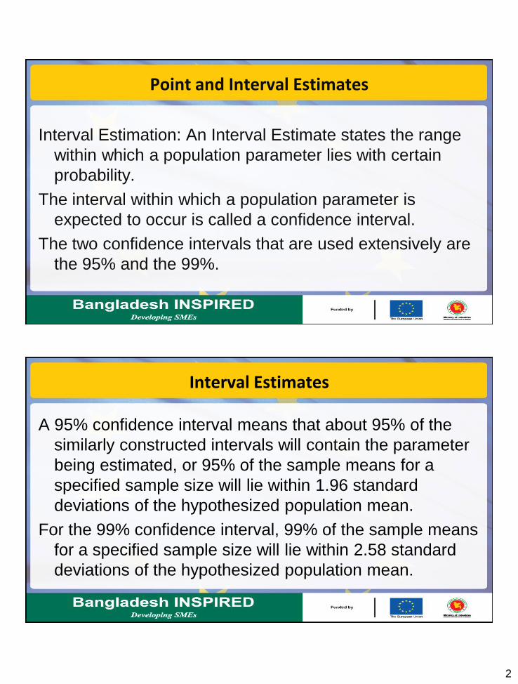
Interval Estimation: An Interval Estimate states the range
within which a population parameter lies with certain
probability.
The interval within which a population parameter is
expected to occur is called a confidence interval.
The two confidence intervals that are used extensively are
the 95% and the 99%.
Interval Estimates
A 95% confidence interval means that about 95% of the
similarly constructed intervals will contain the parameter
being estimated, or 95% of the sample means for a
specified sample size will lie within 1.96 standard
deviations of the hypothesized population mean.
For the 99% confidence interval, 99% of the sample means
for a specified sample size will lie within 2.58 standard
deviations of the hypothesized population mean.
3
Standard Error of the Sample Means
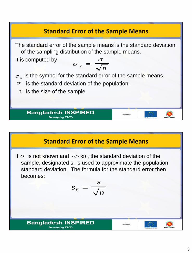
The standard error of the sample means is the standard deviation
of the sampling distribution of the sample means.
It is computed by
is the symbol for the standard error of the sample means.
is the standard deviation of the population.
n is the size of the sample.
xn
x
Standard Error of the Sample Means
If is not known and , the standard deviation of the
sample, designated s, is used to approximate the population
standard deviation. The formula for the standard error then
becomes:
n30
ss
nx
4
95% and 99% Confidence Intervals for µ
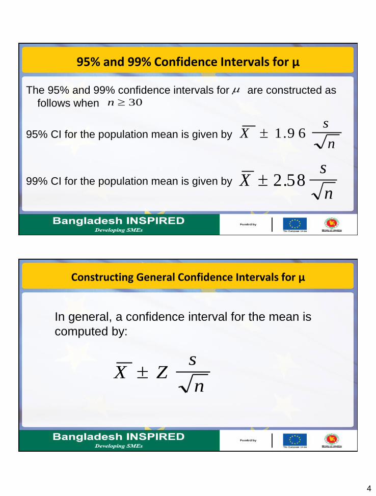
The 95% and 99% confidence intervals for are constructed as
follows when
95% CI for the population mean is given by
99% CI for the population mean is given by
n 30
Xs
n 1 9 6.
Xs
n 2 58.
Constructing General Confidence Intervals for µ
In general, a confidence interval for the mean is
computed by:
X Zs
n
5
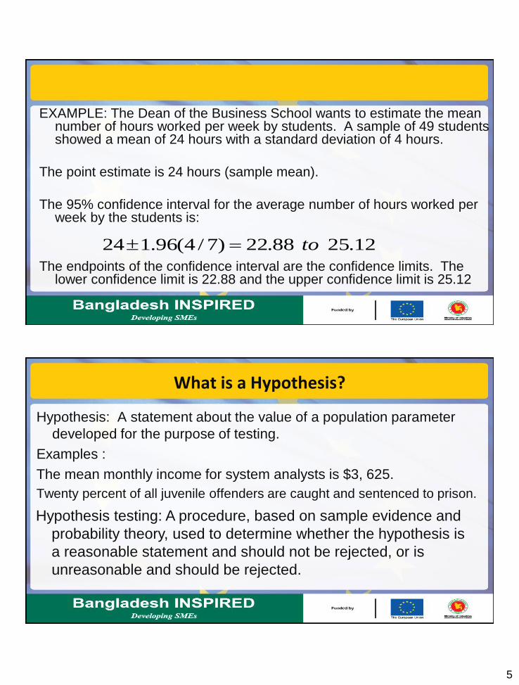
EXAMPLE: The Dean of the Business School wants to estimate the mean number of hours worked per week by students. A sample of 49 students showed a mean of 24 hours with a standard deviation of 4 hours.
The point estimate is 24 hours (sample mean).
The 95% confidence interval for the average number of hours worked per week by the students is:
The endpoints of the confidence interval are the confidence limits. The lower confidence limit is 22.88 and the upper confidence limit is 25.12
12.25 88.22)7/4(96.124 to
What is a Hypothesis?
Hypothesis: A statement about the value of a population parameter
developed for the purpose of testing.
Examples :
The mean monthly income for system analysts is $3, 625.
Twenty percent of all juvenile offenders are caught and sentenced to prison.
Hypothesis testing: A procedure, based on sample evidence and
probability theory, used to determine whether the hypothesis is
a reasonable statement and should not be rejected, or is
unreasonable and should be rejected.
6
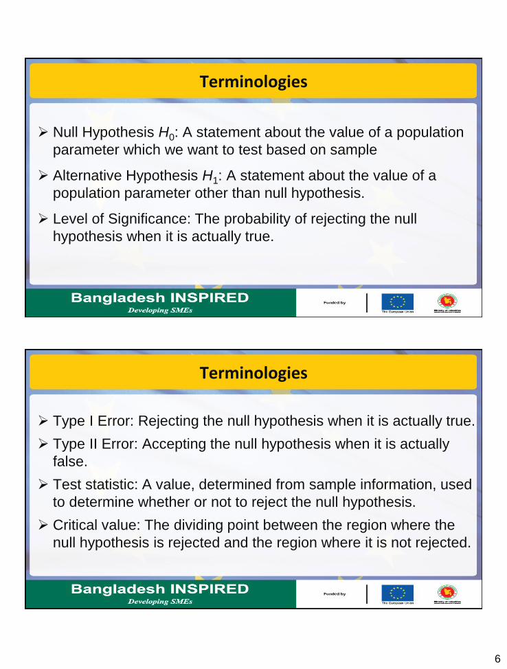
Terminologies
Null Hypothesis H0: A statement about the value of a population
parameter which we want to test based on sample
Alternative Hypothesis H1: A statement about the value of a
population parameter other than null hypothesis.
Level of Significance: The probability of rejecting the null
hypothesis when it is actually true.
Terminologies
Type I Error: Rejecting the null hypothesis when it is actually true.
Type II Error: Accepting the null hypothesis when it is actually
false.
Test statistic: A value, determined from sample information, used
to determine whether or not to reject the null hypothesis.
Critical value: The dividing point between the region where the
null hypothesis is rejected and the region where it is not rejected.
7
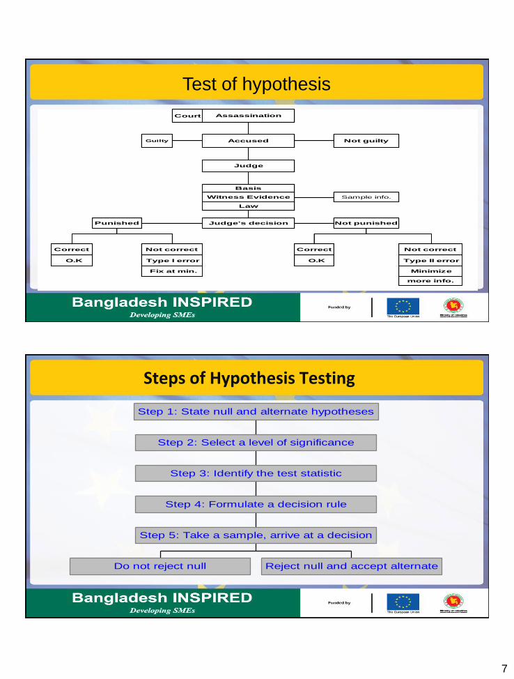
Court
Minimize
O.K
Correct Not correct
Type I error
Correct Not correct
O.K Type II error
Assassination
Judge
Basis
Punished
more info.
Guilty
Witness Evidence Sample info.
Not guilty
Law
Judge's decision
Accused
Not punished
Fix at min.
Test of hypothesis
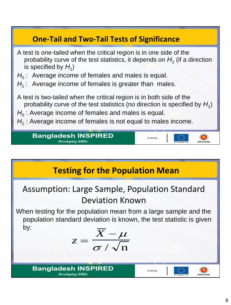
Steps of Hypothesis Testing
Do not reject null Reject null and accept alternate
Step 5: Take a sample, arrive at a decision
Step 4: Formulate a decision rule
Step 3: Identify the test statistic
Step 2: Select a level of significance
Step 1: State null and alternate hypotheses
8
One-Tail and Two-Tail Tests of Significance
A test is one-tailed when the critical region is in one side of the probability curve of the test statistics, it depends on H1 (if a direction is specified by H1)
H0 : Average income of females and males is equal.
H1 : Average income of females is greater than males.
A test is two-tailed when the critical region is in both side of the probability curve of the test statistics (no direction is specified by H1)
H0 : Average income of females and males is equal.
H1 : Average income of females is not equal to males income.
Testing for the Population Mean
When testing for the population mean from a large sample and the
population standard deviation is known, the test statistic is given
by:
zX
/ n
Assumption: Large Sample, Population Standard Deviation Known
9
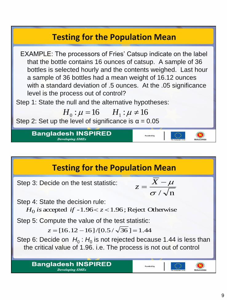
EXAMPLE: The processors of Fries’ Catsup indicate on the label
that the bottle contains 16 ounces of catsup. A sample of 36
bottles is selected hourly and the contents weighed. Last hour
a sample of 36 bottles had a mean weight of 16.12 ounces
with a standard deviation of .5 ounces. At the .05 significance
level is the process out of control?
Step 1: State the null and the alternative hypotheses:
Step 2: Set up the level of significance is α = 0.05
Testing for the Population Mean
16: 16: 10 HH
Step 3: Decide on the test statistic:
Step 4: State the decision rule:
Step 5: Compute the value of the test statistic:
Step 6: Decide on H0 : H0 is not rejected because 1.44 is less than
the critical value of 1.96. i.e. The process is not out of control
OtherwiseReject ; 96.1 1.96 - accepted 0 zifisH
44.1]36/5.0/[]1612.16[ z
n/
Xz
Testing for the Population Mean
10
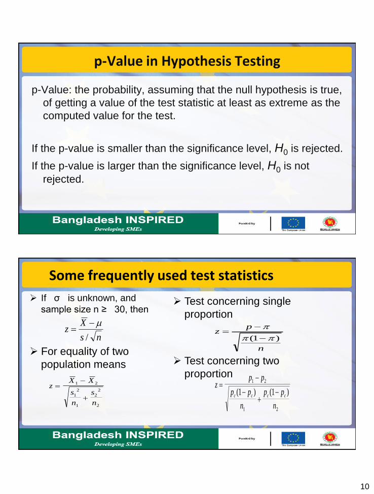
p-Value in Hypothesis Testing
p-Value: the probability, assuming that the null hypothesis is true,
of getting a value of the test statistic at least as extreme as the
computed value for the test.
If the p-value is smaller than the significance level, H0 is rejected.
If the p-value is larger than the significance level, H0 is not
rejected.
Some frequently used test statistics
If σ is unknown, and
sample size n ≥ 30, then
For equality of two
population means
z
X X
s
n
s
n
1 2
1
2
1
2
2
2
ns
Xz
/
n
pz
)1(
zp p
p p
n
p p
n
c c c c
1 2
1 2
1 1( ) ( )
Test concerning single
proportion
Test concerning two
proportion
11
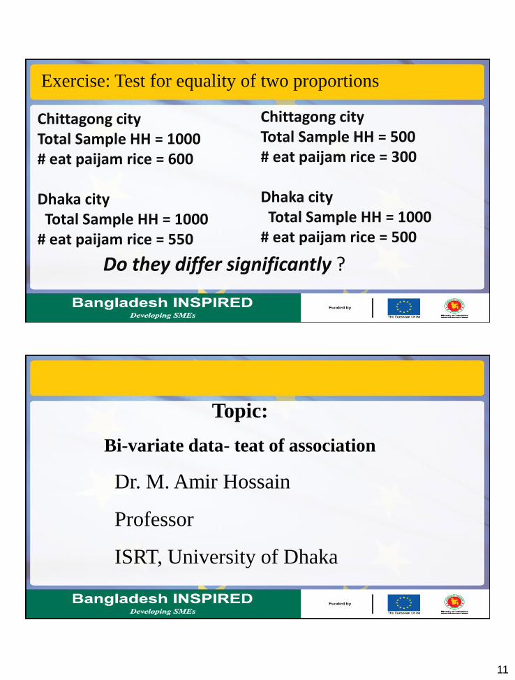
Exercise: Test for equality of two proportions
Chittagong city Total Sample HH = 1000 # eat paijam rice = 600 Dhaka city Total Sample HH = 1000 # eat paijam rice = 550
Chittagong city Total Sample HH = 500 # eat paijam rice = 300 Dhaka city Total Sample HH = 1000 # eat paijam rice = 500
Do they differ significantly ?
Topic:
Bi-variate data- teat of association
Dr. M. Amir Hossain
Professor
ISRT, University of Dhaka
12
Cross Tables
Cross Tables: list the number of observations for every combination of values for two variables concerned is cross tables or bi-variate tables
If both the variables are categorical or ordinal variables (Qualitative ) then it will be a contingency table.
If both the variables are interval or ratio variables (Quantitative) then it will be a bi-variate table.
If there are r categories for the first variable (rows) and c categories for the second variable (columns), the table is called an r x c cross table
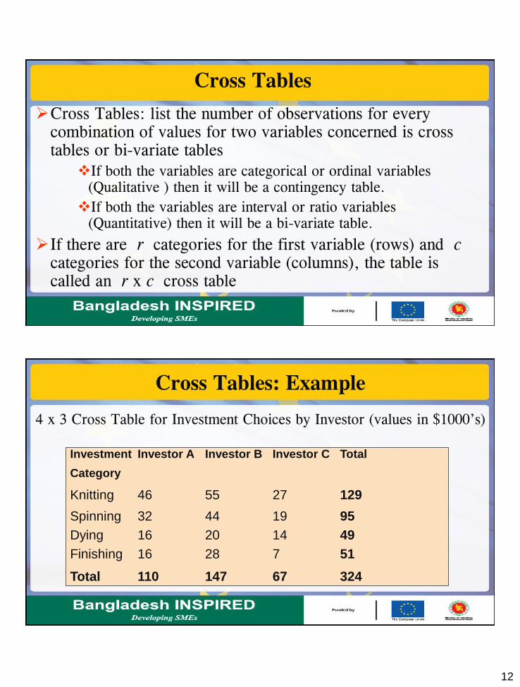
Cross Tables: Example
4 x 3 Cross Table for Investment Choices by Investor (values in $1000’s)
Investment Investor A Investor B Investor C Total
Category
Knitting 46 55 27 129 Spinning 32 44 19 95 Dying 16 20 14 49 Finishing 16 28 7 51 Total 110 147 67 324
13
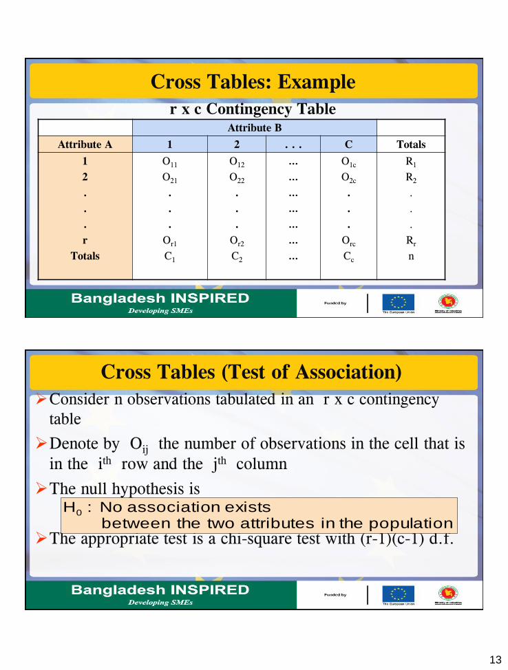
Cross Tables: Example
r x c Contingency Table Attribute B
Attribute A 1 2 . . . C Totals
1
2
.
.
.
r
Totals
O11
O21
.
.
.
Or1
C1
O12
O22
.
.
.
Or2
C2
…
…
…
…
…
…
…
O1c
O2c
.
.
.
Orc
Cc
R1
R2
.
.
.
Rr
n
Cross Tables (Test of Association)
Consider n observations tabulated in an r x c contingency
table
Denote by Oij the number of observations in the cell that is
in the ith row and the jth column
The null hypothesis is
The appropriate test is a chi-square test with (r-1)(c-1) d.f. population the in attributes two the between
exists nassociatio No :H0
14
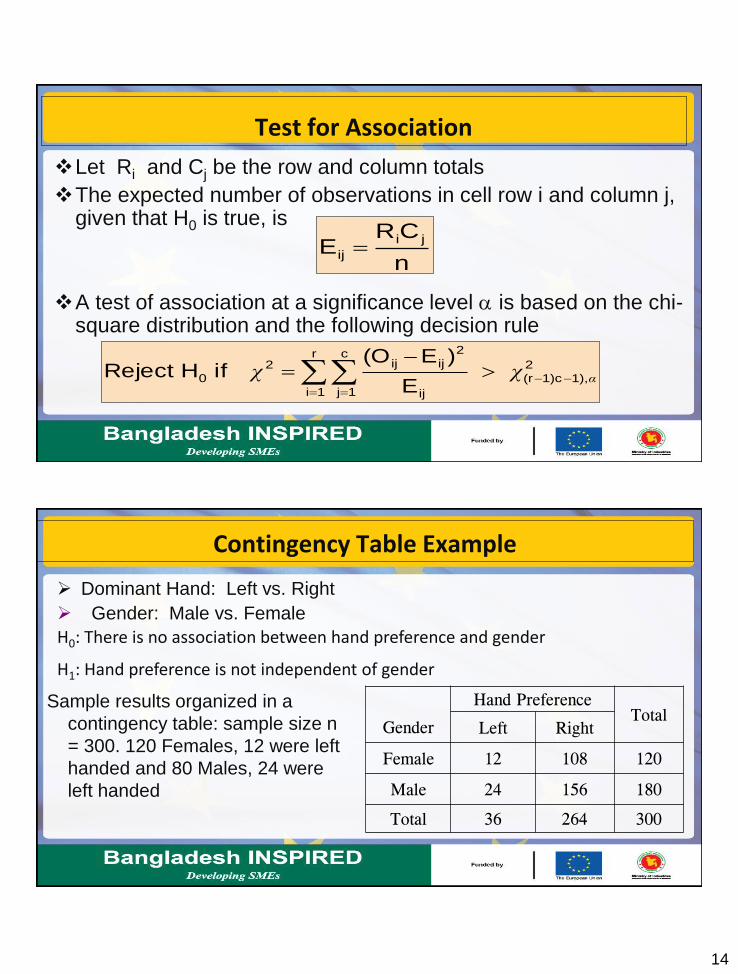
Test for Association
Let Ri and Cj be the row and column totals
The expected number of observations in cell row i and column j, given that H0 is true, is
A test of association at a significance level is based on the chi-square distribution and the following decision rule
2
1),1)c(r
r
1i
c
1j ij
2
ijij2
0E
)E(O if H Reject αχχ
n
CRE
ji
ij
Contingency Table Example
Dominant Hand: Left vs. Right
Gender: Male vs. Female
H0: There is no association between hand preference and gender
H1: Hand preference is not independent of gender
Sample results organized in a
contingency table: sample size n
= 300. 120 Females, 12 were left
handed and 80 Males, 24 were
left handed
Gender
Hand Preference Total
Left Right
Female 12 108 120
Male 24 156 180
Total 36 264 300
15
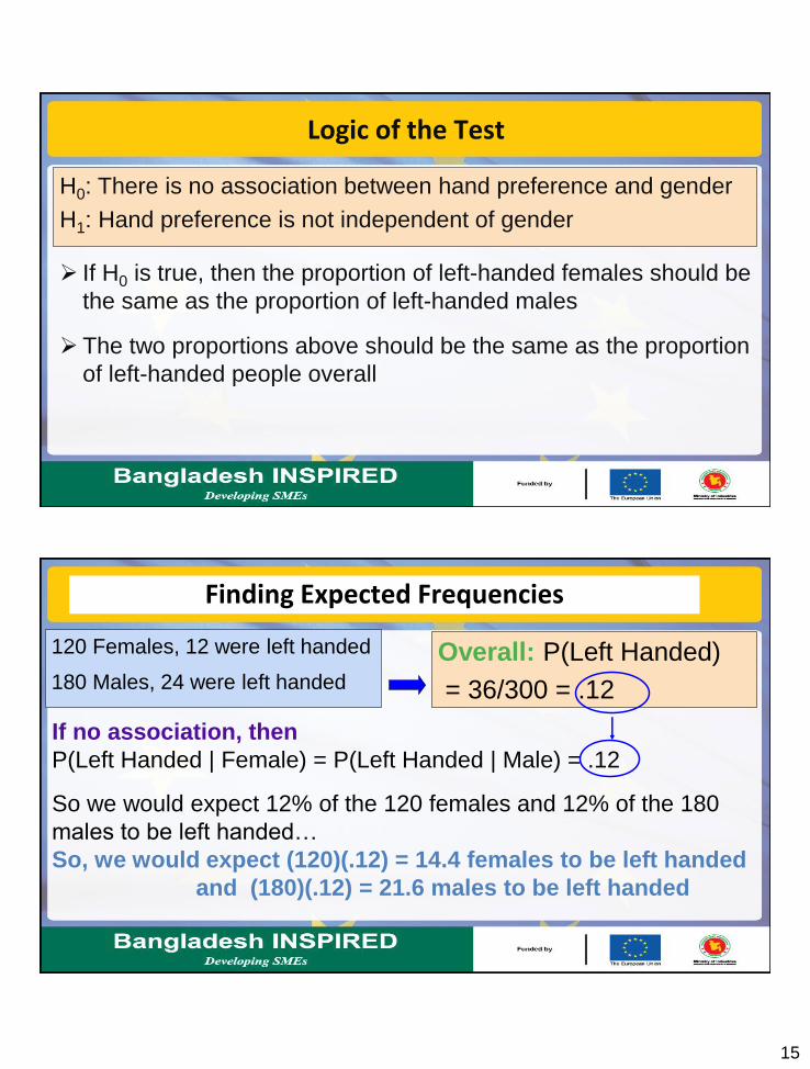
Logic of the Test
If H0 is true, then the proportion of left-handed females should be
the same as the proportion of left-handed males
The two proportions above should be the same as the proportion
of left-handed people overall
H0: There is no association between hand preference and gender
H1: Hand preference is not independent of gender
Finding Expected Frequencies
Overall: P(Left Handed)
= 36/300 = .12
120 Females, 12 were left handed
180 Males, 24 were left handed
If no association, then
P(Left Handed | Female) = P(Left Handed | Male) = .12
So we would expect 12% of the 120 females and 12% of the 180
males to be left handed…
So, we would expect (120)(.12) = 14.4 females to be left handed
and (180)(.12) = 21.6 males to be left handed
16
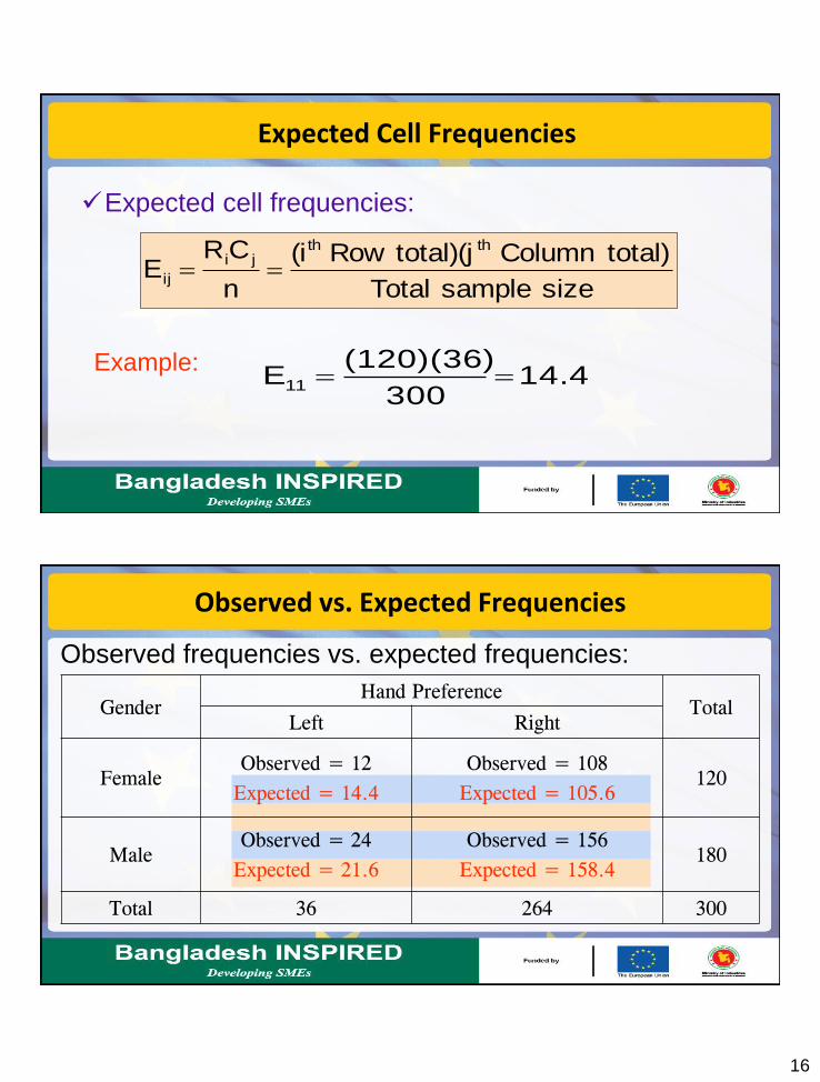
Expected Cell Frequencies
Expected cell frequencies:
size sample Total
total) Column total)(jRow (i
n
CRE
ththji
ij
14.4300
(120)(36)E11
Example:
Observed vs. Expected Frequencies
Observed frequencies vs. expected frequencies:
Gender
Hand Preference Total
Left Right
Female Observed = 12
Expected = 14.4
Observed = 108
Expected = 105.6 120
Male Observed = 24
Expected = 21.6
Observed = 156
Expected = 158.4 180
Total 36 264 300
17
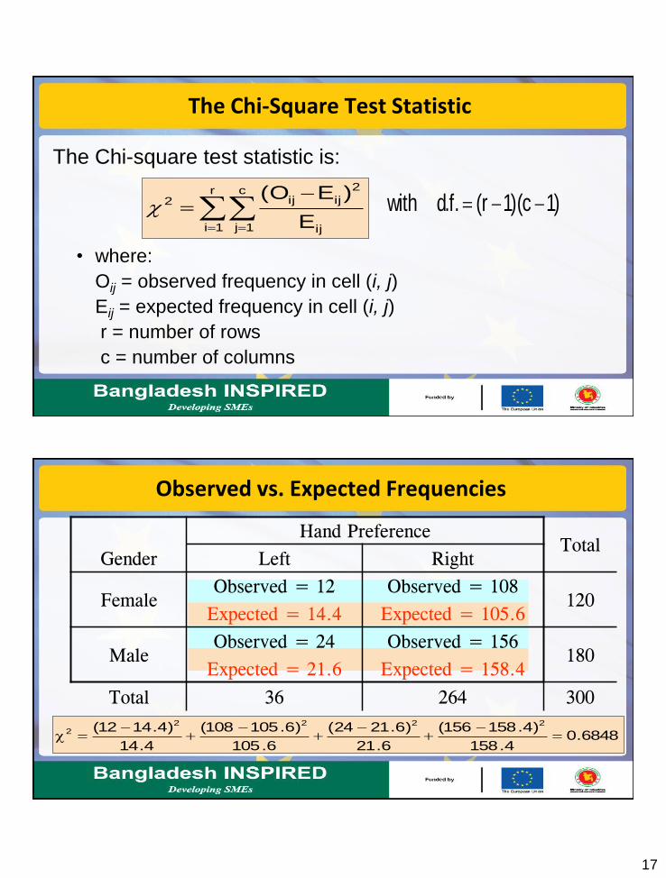
The Chi-Square Test Statistic
• where:
Oij = observed frequency in cell (i, j)
Eij = expected frequency in cell (i, j)
r = number of rows
c = number of columns
r
1i
c
1j ij
2
ijij2
E
)E(O
The Chi-square test statistic is:
)1c)(1r(.f.d with
Observed vs. Expected Frequencies
Gender
Hand Preference Total
Left Right
Female Observed = 12
Expected = 14.4
Observed = 108
Expected = 105.6 120
Male Observed = 24
Expected = 21.6
Observed = 156
Expected = 158.4 180
Total 36 264 300
6848.04.158
)4.158156(
6.21
)6.2124(
6.105
)6.105108(
4.14
)4.1412( 22222
18
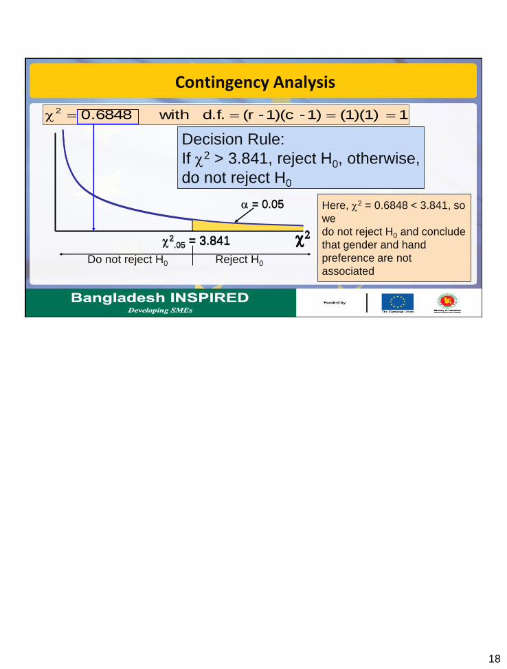
Contingency Analysis
2 2.05 = 3.841
Reject H0
= 0.05
Decision Rule:
If 2 > 3.841, reject H0, otherwise,
do not reject H0
1(1)(1)1)-1)(c-(r d.f. with6848.02
Do not reject H0
Here, 2 = 0.6848 < 3.841, so
we
do not reject H0 and conclude
that gender and hand
preference are not
associated
2 2.05 = 3.841
= 0.05