database management system - wordpress.com · compared to database management system. data...
TRANSCRIPT
DATABASE MANAGEMENT SYSTEM
S u b j e c t C o o r d i n a t o r : P r o f . A s h i s h P r a j a p a t i C E - 1 S u b j e c t f a c u l t y : P r o f . A m i t P a r m a r C E - 2 S u b j e c t f a c u l t y : P r o f . P r a t i k P a t e l
C E - 3 S u b j e c t f a c u l t y : P r o f . K a v i t a T i w a r i
B A B A R I A I N S T I T U T E O F T E C H N O L O G Y C . S . E D E P A R T M E N T
1. Explain disadvantages of file system (file processing
systems) compare to Database management system. OR Explain disadvantages of conventional file-based system compared to Database management system.
Data Redundancy It is possible that the same information may be duplicated in different files. This leads to
data redundancy.
Data redundancy results in memory wastage. For example, consider that some customers have both kinds of accounts - saving and
current. In this case, data about customers - name, address, e-mail, contact number -
will be duplicated in both files, file for saving accounts and file for current accounts. This leads to requirement of higher storage space. In other words, same information will be stored in two different locations (files). And, it wastes memory.
Data Inconsistency Due to data redundancy, it is possible that data may not be in consistent state. For example, consider that an address of some customer changes. And, that customer
has both kinds of accounts. Now, it is possible that this changed address is updated in only one file, leaving address in other file as it is. As a result of this, same customer will have two different addresses in two different files, making data inconsistent.
Difficulty in Accessing Data Accessing data is not convenient and efficient in file processing system. For example, suppose, there is a program to find information about all customers. But,
what if there is a need to find out all customers from some particular city. In this case, there are two choices here: One, find out all customers using available program, and then extract the needed customers manually. Second, develop new program to get required information. Both options are not satisfactory.
For each and every different kind of data access, separate programs are required. This is neither convenient nor efficient.
Limited Data Sharing Data are scattered in various files. Different files may have different formats. And these files may be stored in different
folders (directories) may be of different computers of different departments.
So, due to this data isolation, it is difficult to share data among different applications.
Integrity Problems Data integrity means that the data contained in the database is both correct and
consistent. For this purpose, the data stored in database must satisfy certain types of constraints (rules).
For example, a balance for any account must not be less than zero. Such constraints are
enforced in the system by adding appropriate code in application programs. But, when new constraints are added, such as balance should not be less than Rs. 5000, application programs need to be changed. But, it is not an easy task to change programs whenever required.
Atomicity Problems Any operation on database must be atomic. This means, operation completes either
100% or 0%. For example, a fund transfer from one account to another must happen in its entirely.
But, computer systems are vulnerable to failure, such as system crash, virus attack. If a system failure occurs during the execution of fund transfer operation, it may possible that amount to be transferred, say, Rs. 500, is debited from one account, but is not credited to another account.
This leaves database in inconsistent state. But, it is difficult to ensure atomicity in a file processing system.
Concurrent Access Anomalies Multiple users are allowed to access data simultaneously (concurrently). This is for the
sake of better performance and faster response. Consider an operation to debit (withdrawal) an account. The program reads the old
balance, calculates the new balance, and writes new balance back to database. Suppose an account has a balance of Rs. 5000. Now, a concurrent withdrawal of Rs. 1000 and Rs. 2000 may leave the balance Rs. 4000 or Rs. 3000 depending upon their completion time rather than the correct value of Rs. 2000.
Here, concurrent data access should be allowed under some supervision. But, due to lack of co-ordination among different application programs, this is not
possible in file processing systems.
Security Problems Database should be accessible to users in a limited way.
Each user should be allowed to access data concerning his application only. For example, a customer can check balance only for his/her own account. He/She
should not have access for information about other accounts. But, in file processing system, application programs are added in an ad hoc manner by
different programmers. So, it is difficult to enforce such kind of security constraints.
2. Describe functions (responsibility, roles, and duties) of DBA
to handle DBMS. DBA The full name of DBA is Database Administrator. Database Administrator is a person in the organization who controls the design and the
use of database.
Functions or Responsibilities of DBA are as under: Schema Definition DBA defines the logical schema of the database.
A schema refers to the overall logical structure of the database. According to this schema, database will be designed to store required data for an
organization.
Storage Structure and Access Method Definition DBA decides how the data is to be represented in the database. Based on this, storage structure of the database and access methods of data is defined.
Defining Security and Integrity Constraints DBA decides various security and integrity constraints.
DDL provides facilities to specifying such constraints.
Granting of Authorization for Data Access The DBA determines which user needs access to which part of the database. According to this, various types of authorizations (permissions) are granted to different
users.
This is required to prevent unauthorized access of a database.
Liaison with Users DBA is responsible to provide necessary data to user.
User should be able to write the external schema, using DDL.
Assisting Application Programmers DBA provides assistance to application programmers to develop application programs.
Monitoring Performance The DBA monitors performance of the system. The DBA ensures that better performance is maintained by making change in physical or
logical schema if required.
Backup and Recovery Database should not be lost or damaged. The task of DBA is to backing up the database on some storage devices such as DVD, CD
or Magnetic Tape or remote servers.
In case of failures, such as flood or virus attack, Database is recovered from this backup.
3. Explain three levels ANSI SPARC Database System.
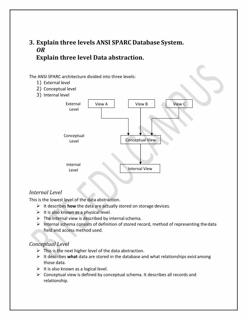
OR Explain three level Data abstraction. The ANSI SPARC architecture divided into three levels:
1) External level
2) Conceptual level
3) Internal level
External Level
Conceptual Level
Internal
Level
Internal Level This is the lowest level of the data abstraction.
It describes how the data are actually stored on storage devices.
It is also known as a physical level.
The internal view is described by internal schema. Internal schema consists of definition of stored record, method of representing the data
field and access method used.
Conceptual Level This is the next higher level of the data abstraction. It describes what data are stored in the database and what relationships exist among
those data.
It is also known as a logical level. Conceptual view is defined by conceptual schema. It describes all records and
relationship.
View B View A View C
Conceptual View
Internal View
External Level This is the highest level of data abstraction.
It is also known as view level.
It describes only part of the entire database that a particular end user requires.
External view is describes by external schema. External schema consists of definition of logical records, relationship in the external
view and method of deriving the objects from the conceptual view.
This object includes entities, attributes and relationship.
4. Explain Data Independence. Data Independence Data independency is the ability to modify a schema definition in one level without
affecting a schema definition in the next higher level.
Types of data independence Physical data independence
Logical data independence
Physical data independence Physical data independence allows changing in physical storage devices or organization
of file without change in the conceptual view or external view.
Modifications at the internal level are occasionally necessary to improve performance.
Physical data independence separates conceptual level from the internal level.
It is easy to achieve physical data independence.
Logical data independence Logical data independence is the ability to modify the conceptual schema without
requiring any change in application programs.
Conceptual schema can be changed without affecting the existing external schema. Modifications at the logical level are necessary whenever the logical structure of the
database is altered.
Logical data independence separates external level from the conceptual view.
It is difficult to achieve logical data independence.
5. Explain different database users. There are four different database users.
Application programmers These users are computer professionals who write application programs using some
tools.
Sophisticated users These users interact with system without writing program. They form their request in a
database query language.
Specialized users These users write specialized database applications that do not fit into the traditional
data processing framework.
Naive users These users are unsophisticated users who have very less knowledge of database
system. These users interact with the system by using one of the application programs that have
been written previously. Examples, people accessing database over the web, bank tellers, clerical staff etc.
6. Explain Database System Architecture. Components of a DBMS These functional units of a database system can be divided into two parts:
1. Query Processor Units (Components) 2. Storage Manager Units
Query Processor Units: Query processor units deal with execution of DDL and DML statements.
DDL Interpreter — Interprets DDL statements into a set of tables containing metadata.
DML Compiler — Translates DML statements into low level instructions that the query evaluation engine understands.
Embedded DML Pre-compiler — Converts DML statements embedded in an application program into normal procedure caIls in the host language.
Query Evaluation Engine — Executes low level instructions generated by DML compiler.
Storage Manager Units: Storage manager units provide interface between the low level data stored in database and the application programs & queries submitted to the system.
Authorization Manager — Checks the authority of users to access data.
Integrity Manager — Checks for the satisfaction of the integrity constraints.
Transaction Manager — Preserves atomicity and controls concurrency. File Manager — Manages allocation of space on disk storage. Buffer Manager — Fetches data from disk storage to memory for being used.
In addition to these functional units, several data structures are required to implement
physical storage system. These are described below:
Data Files — To store user data.
Data Dictionary and System Catalog — To store metadata. It is used heavily, almost for each and every data manipulation operation. So, it should be accessed efficiently.
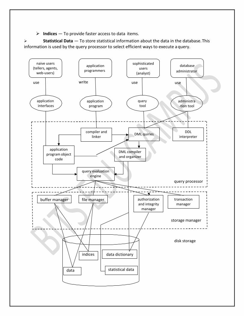
Indices — To provide faster access to data items.
Statistical Data — To store statistical information about the data in the database. This information is used by the query processor to select efficient ways to execute a query.
naive users (tellers, agents,
web-users)
application programmers
sophisticated users
(analyst)
database
administrator
use write use use
application interfaces
application program
query tool
administra -tion tool
compiler and linker
application
program object code
DML compiler and organizer
query processor
storage manager
disk storage
indices
data
buffer manager file manager authorization and integrity
manager
transaction manager
DML quiries DDL
interpreter
query evaluation engine
data dictionary
statistical data
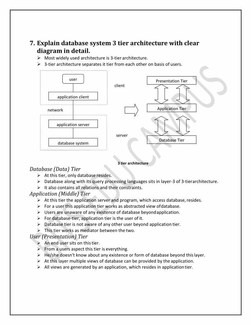
7. Explain database system 3 tier architecture with clear diagram in detail. Most widely used architecture is 3-tier architecture.
3-tier architecture separates it tier from each other on basis of users.
client
server
3 tier architecture
Database (Data) Tier At this tier, only database resides. Database along with its query processing languages sits in layer-3 of 3-tier architecture. It also contains all relations and their constraints.
Application (Middle) Tier At this tier the application server and program, which access database, resides. For a user this application tier works as abstracted view of database. Users are unaware of any existence of database beyond application. For database-tier, application tier is the user of it. Database tier is not aware of any other user beyond application tier. This tier works as mediator between the two.
User (Presentation) Tier An end user sits on this tier. From a users aspect this tier is everything. He/she doesn't know about any existence or form of database beyond this layer. At this layer multiple views of database can be provided by the application. All views are generated by an application, which resides in application tier.
Application Tier
user
application client
network
application server
database system
Presentation Tier
Database Tier
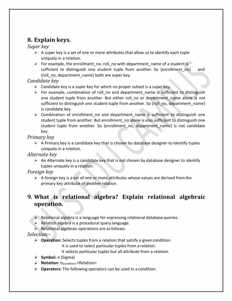
8. Explain keys. Super key
A super key is a set of one or more attributes that allow us to identify each tuple uniquely in a relation.
For example, the enrollment_no, roll_no with department_name of a student is sufficient to distinguish one student tuple from another. So {enrollment_no} and
{roll_no, department_name} both are super key.
Candidate key Candidate key is a super key for which no proper subset is a super key. For example, combination of roll_no and department_name is sufficient to distinguish
one student tuple from another. But either roll_no or department_name alone is not sufficient to distinguish one student tuple from another. So {roll_no, department_name} is candidate key.
Combination of enrollment_no and department_name is sufficient to distinguish one student tuple from another. But enrollment_no alone is also sufficient to distinguish one student tuple from another. So {enrollment_no, department_name} is not candidate key.
Primary key A Primary key is a candidate key that is chosen by database designer to identify tuples
uniquely in a relation.
Alternate key An Alternate key is a candidate key that is not chosen by database designer to identify
tuples uniquely in a relation.
Foreign key A foreign key is a set of one or more attributes whose values are derived from the
primary key attribute of another relation.
9. What is relational algebra? Explain relational algebraic
operation.
Relational algebra is a language for expressing relational database queries. Relation algebra is a procedural query language. Relational algebraic operations are as follows:
Selection:- Operation: Selects tuples from a relation that satisfy a given condition.
It is used to select particular tuples from a relation.It selects particular tuples but all attribute from a relation.
Symbol: σ (Sigma)
Notation: σ(condition) <Relation>
Operators: The following operators can be used in a condition.
=, ?, <, >, <=,>=, Λ(AND), ∨(OR)
Consider following table
Student
Rno Name Dept CPI
101 Ramesh CE 8
108 Mahesh EC 6
109 Amit CE 7 125 Chetan CI 8
138 Mukesh ME 7
128 Reeta EC 6
133 Anita CE 9
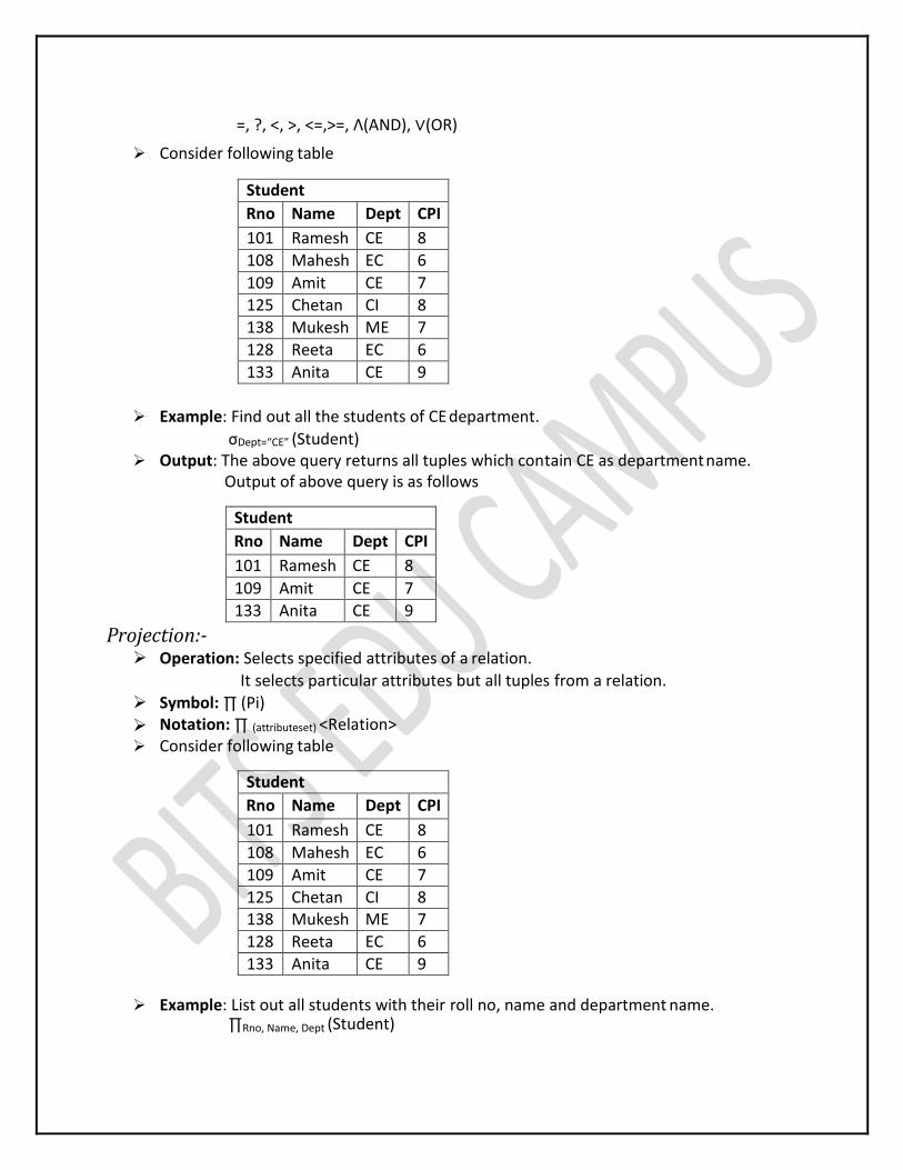
Example: Find out all the students of CE department.
σDept=“CE” (Student) Output: The above query returns all tuples which contain CE as department name.
Output of above query is as follows
Student
Rno Name Dept CPI
101 Ramesh CE 8
109 Amit CE 7
133 Anita CE 9
Projection:- Operation: Selects specified attributes of a relation.
It selects particular attributes but all tuples from a relation. Symbol: ∏ (Pi)
Notation: ∏ (attributeset) <Relation> Consider following table
Student
Rno Name Dept CPI
101 Ramesh CE 8
108 Mahesh EC 6
109 Amit CE 7
125 Chetan CI 8 138 Mukesh ME 7
128 Reeta EC 6
133 Anita CE 9
Example: List out all students with their roll no, name and department name.∏Rno, Name, Dept (Student)
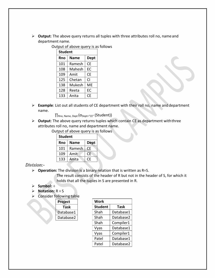
Output: The above query returns all tuples with three attributes roll no, name and department name.
Output of above query is as follows
Student
Rno Name Dept
101 Ramesh CE
108 Mahesh EC 109 Amit CE 125 Chetan CI
138 Mukesh ME
128 Reeta EC
133 Anita CE
Example: List out all students of CE department with their roll no, name and department name.
∏Rno, Name, Dept (σDept=“CE” (Student)) Output: The above query returns tuples which contain CE as department with three
attributes roll no, name and department name.Output of above query is as follows
Student
Rno Name Dept
101 Ramesh CE
109 Amit CE
133 Anita CE
Division:- Operation: The division is a binary relation that is written as R÷S.
The result consists of the header of R but not in the header of S, for which it holds that all the tuples in S are presented in R.
Symbol: ÷ Notation: R ÷ S Consider following table
Project
Task Database1
Database2
Work
Student Task
Shah Database1
Shah Database2
Shah Compiler1 Vyas Database1
Vyas Compiler1 Patel Database1
Patel Database2
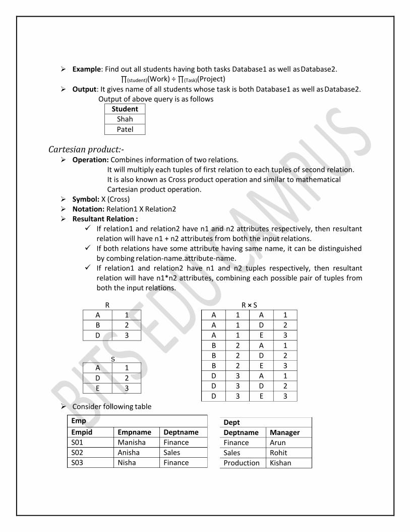
Example: Find out all students having both tasks Database1 as well as Database2.∏(student)(Work) ÷ ∏(Task)(Project)
Output: It gives name of all students whose task is both Database1 as well as Database2. Output of above query is as follows
Student Shah
Patel
Cartesian product:- Operation: Combines information of two relations.
It will multiply each tuples of first relation to each tuples of second relation. It is also known as Cross product operation and similar to mathematical Cartesian product operation.
Symbol: X (Cross) Notation: Relation1 X Relation2 Resultant Relation :
If relation1 and relation2 have n1 and n2 attributes respectively, then resultant relation will have n1 + n2 attributes from both the input relations.
If both relations have some attribute having same name, it can be distinguished by combing relation-name.attribute-name.
If relation1 and relation2 have n1 and n2 tuples respectively, then resultant relation will have n1*n2 attributes, combining each possible pair of tuples from both the input relations.
R R × S A 1 B 2
D 3
S
A 1
D 2
E 3
Consider following table
Emp
Empid Empname Deptname
S01 Manisha Finance
S02 Anisha Sales S03 Nisha Finance
Dept
Deptname Manager Finance Arun
Sales Rohit
Production Kishan
A 1 A 1
A 1 2 A 1 3
B 2 A 1 B 2 2
B 2 3
3 A 1 3 2
3 3

Example:
Emp × Dept
Empid Empname Emp.Deptname Dept.Deptname Manager
S01 Manisha Finance Finance Arun
S01 Manisha Finance Sales Rohit
S01 Manisha Finance Production Kishan S02 Anisha Sales Finance Arun
S02 Anisha Sales Sales Rohit
S02 Anisha Sales Production Kishan
S03 Nisha Finance Finance Arun
S03 Nisha Finance Sales Rohit
S03 Nisha Finance Production Kishan
Join:- Natural Join Operation (⋈) Operation: Natural join will retrieve information from multiple relations. It works in
three steps.1. It performs Cartesian product 2. Then it finds consistent tuples and inconsistent tuples are deleted 3. Then it deletes duplicate attributes
Symbol: ⋈ Notation: Relation1 ⋈ Relation2 Consider following table
Example:
Emp ⋈ Dept
Empid Empname Deptname Manager
S01 Manisha Finance Arun
S02 Anisha Sales Rohit
S03 Nisha Finance Arun
The Outer Join Operation An outer join does not require each record in the two joined tables to have a matching
record.
Emp
Empid Empname Deptname
S01 Manisha Finance S02 Anisha Sales
S03 Nisha Finance
Dept Deptame Manager
Finance Arun
Sales Rohit
Production Kishan
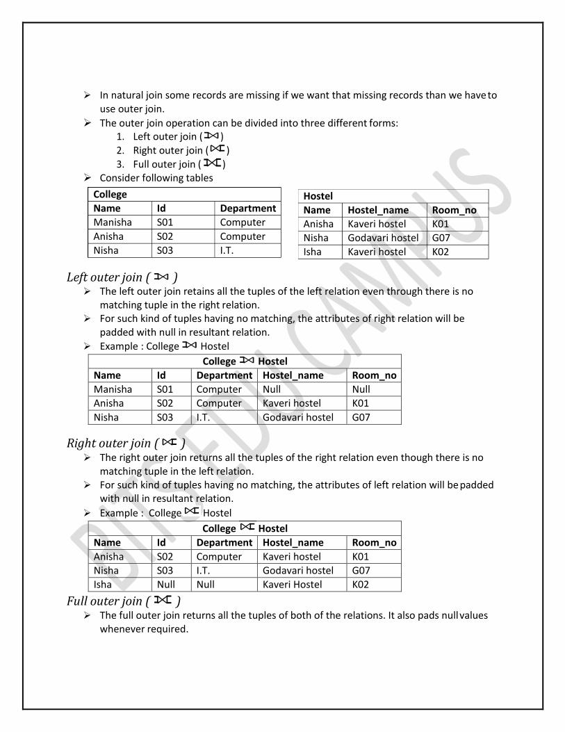
In natural join some records are missing if we want that missing records than we have to use outer join.
The outer join operation can be divided into three different forms:1. Left outer join ( ) 2. Right outer join ( ) 3. Full outer join ( )
Consider following tables
Left outer join ( ) The left outer join retains all the tuples of the left relation even through there is no
matching tuple in the right relation. For such kind of tuples having no matching, the attributes of right relation will be
padded with null in resultant relation.
Example : College Hostel
College Hostel
Name Id Department Hostel_name Room_no
Manisha S01 Computer Null Null Anisha S02 Computer Kaveri hostel K01
Nisha S03 I.T. Godavari hostel G07
Right outer join ( ) The right outer join returns all the tuples of the right relation even though there is no
matching tuple in the left relation. For such kind of tuples having no matching, the attributes of left relation will be padded
with null in resultant relation.
Example : College Hostel
College Hostel
Name Id Department Hostel_name Room_no
Anisha S02 Computer Kaveri hostel K01 Nisha S03 I.T. Godavari hostel G07
Isha Null Null Kaveri Hostel K02
Full outer join ( ) The full outer join returns all the tuples of both of the relations. It also pads null values
whenever required.
College
Name Id Department
Manisha S01 Computer
Anisha S02 Computer
Nisha S03 I.T.
Hostel
Name Hostel_name Room_no Anisha Kaveri hostel K01 Nisha Godavari hostel G07
Isha Kaveri hostel K02
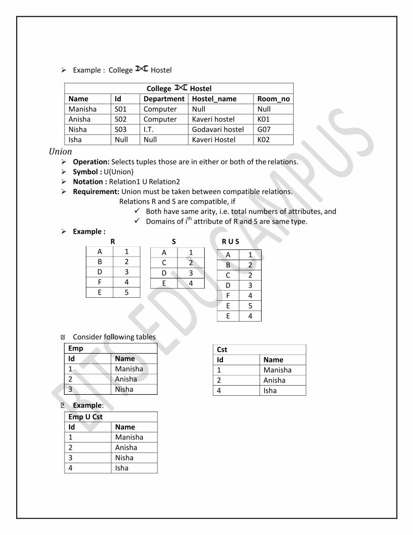
Example : College Hostel
College Hostel
Name Id Department Hostel_name Room_no
Manisha S01 Computer Null Null Anisha S02 Computer Kaveri hostel K01
Nisha S03 I.T. Godavari hostel G07
Isha Null Null Kaveri Hostel K02
Union Operation: Selects tuples those are in either or both of the relations. Symbol : U(Union) Notation : Relation1 U Relation2 Requirement: Union must be taken between compatible relations.
Relations R and S are compatible, if Both have same arity, i.e. total numbers of attributes, and Domains of ith attribute of R and S are same type.
Example : R S R U S
Consider following tables
Example:
Emp U Cst
Id Name 1 Manisha
2 Anisha
3 Nisha
4 Isha
A 1 B 2
3
4
5
A 1
2
3
4
A 1
B 2
2 3
4
5
4
Emp
Id Name
1 Manisha
2 Anisha
3 Nisha
Cst
Id Name
1 Manisha
2 Anisha
4 Isha
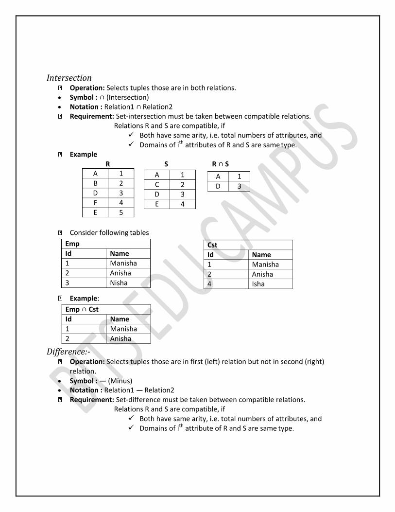
Intersection Operation: Selects tuples those are in both relations. Symbol : ∩ (Intersection) Notation : Relation1 ∩ Relation2 Requirement: Set-intersection must be taken between compatible relations.
Relations R and S are compatible, if Both have same arity, i.e. total numbers of attributes, and Domains of ith attributes of R and S are same type.
Example R S R ∩ S
Consider following tables
Example:
Emp ∩ Cst
Id Name
1 Manisha
2 Anisha
Difference:- Operation: Selects tuples those are in first (left) relation but not in second (right)
relation. Symbol : — (Minus) Notation : Relation1 — Relation2 Requirement: Set-difference must be taken between compatible relations.
Relations R and S are compatible, if Both have same arity, i.e. total numbers of attributes, and Domains of ith attribute of R and S are same type.
A 1
B 2
3 4
5
A 1
2 3
4
A 1
3
Emp
Id Name 1 Manisha
2 Anisha
3 Nisha
Cst
Id Name 1 Manisha
2 Anisha 4 Isha
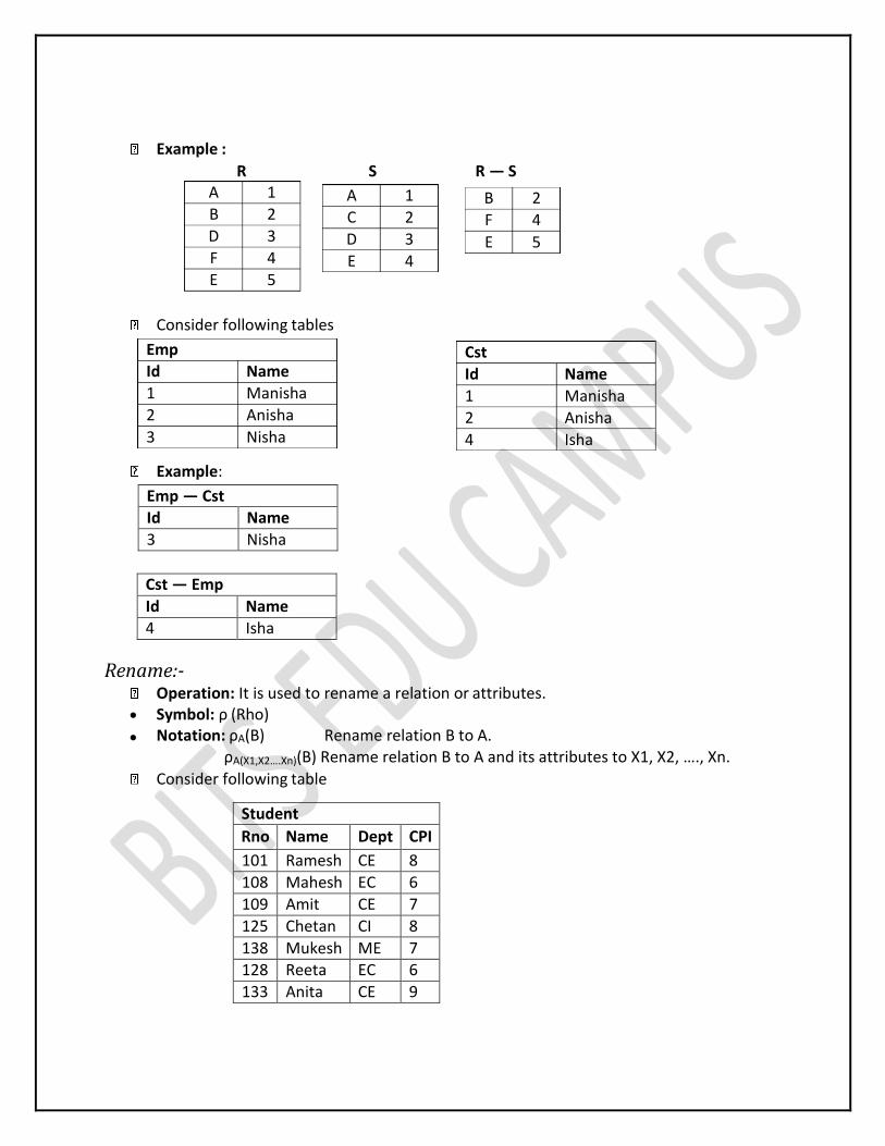
Example : R S R — S
Consider following tables
Example:
Emp — Cst Id Name
3 Nisha
Cst — Emp
Id Name
4 Isha
Rename:- Operation: It is used to rename a relation or attributes. Symbol: ρ (Rho)
Notation: ρA(B) Rename relation B to A.ρA(X1,X2….Xn)(B) Rename relation B to A and its attributes to X1, X2, …., Xn.
Consider following table
Student
Rno Name Dept CPI
101 Ramesh CE 8
108 Mahesh EC 6
109 Amit CE 7
125 Chetan CI 8
138 Mukesh ME 7 128 Reeta EC 6
133 Anita CE 9
A 1
B 2
3
4
5
A 1
2
3
4
B 2
4
5
Emp
Id Name
1 Manisha
2 Anisha
3 Nisha
Cst
Id Name
1 Manisha
2 Anisha
4 Isha

9
51
Example: Find out highest CPI from student table.∏CPI (Student) — ∏A.CPI (σ A.CPI<B.CPI (ρA (Student) X ρB (Student)))
Output: The above query returns highest CPI. Output of above query is as follows
Aggregate Function:- Operation: It takes a more than one value as input and returns a single value as output
(result). Symbol: G
Notation: G function (attribute)(relation) Aggregate functions: Sum, Count, Max, Min, Avg. Consider following table
Student
Rno Name Dept CPI
101 Ramesh CE 8
108 Mahesh EC 6 109 Amit CE 7
125 Chetan CI 8
138 Mukesh ME 7
128 Reeta EC 6
133 Anita CE 9
Example: Find out sum of all students CPI.
G sum (CPI) (Student)Output: The above query returns sum of CPI. Output of above query is as follows
Example: Find out max and min CPI.G max (CPI), min (CPI) (Student) Output: The above query returns sum of CPI. Output of above query is as follows
max min
9 6
CPI
sum
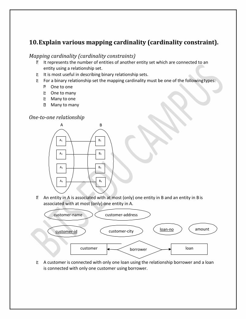
10. Explain various mapping cardinality (cardinality constraint). Mapping cardinality (cardinality constraints)
It represents the number of entities of another entity set which are connected to an entity using a relationship set.
It is most useful in describing binary relationship sets.
For a binary relationship set the mapping cardinality must be one of the following types:
One to one
One to many Many to one
Many to many
One-to-one relationship
A B
An entity in A is associated with at most (only) one entity in B and an entity in B is associated with at most (only) one entity in A.
A customer is connected with only one loan using the relationship borrower and a loan
is connected with only one customer using borrower.
customer-name customer-address
customer-id customer-city loan-no amount
borrower customer loan
A1 B1
A2 B2
A3 B3
A4 B4
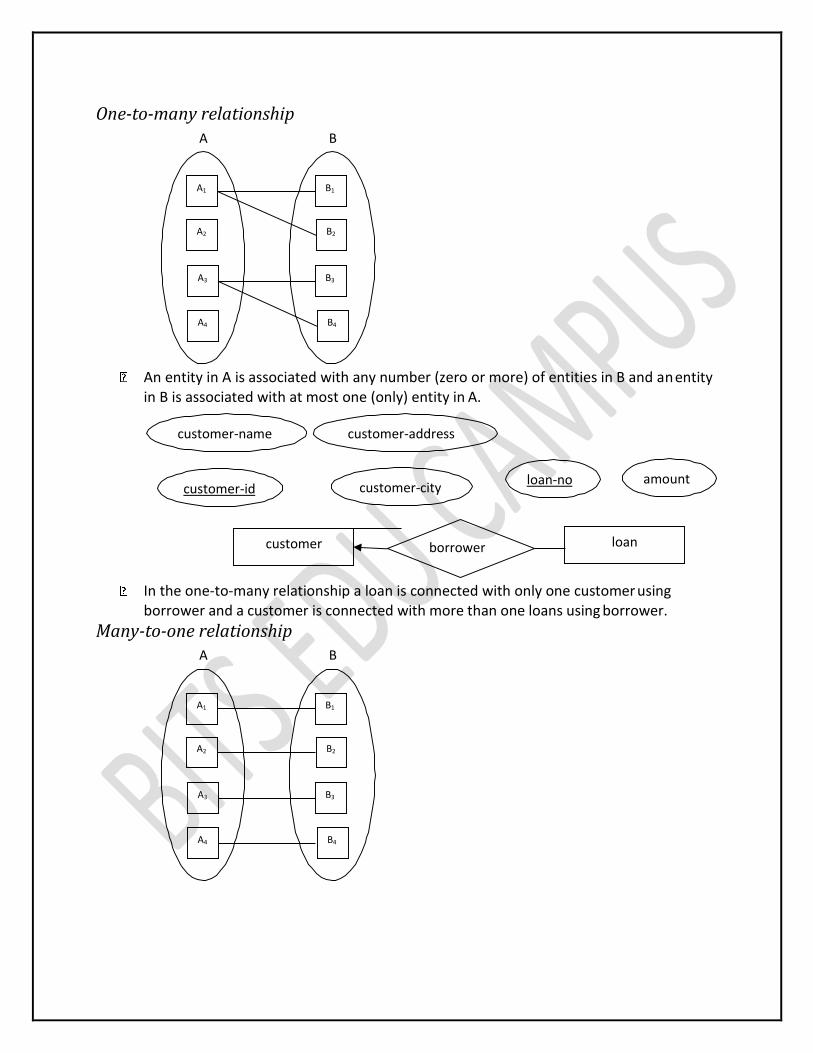
One-to-many relationship A B
An entity in A is associated with any number (zero or more) of entities in B and an entity in B is associated with at most one (only) entity in A.
In the one-to-many relationship a loan is connected with only one customer using borrower and a customer is connected with more than one loans using borrower.
Many-to-one relationship A B
customer-name customer-address
customer-id customer-city loan-no amount
borrower customer loan
A2 B2
A4 B4
A1 B1
A3 B3
A2 B2
A4 B4
A1 B1
A3 B3
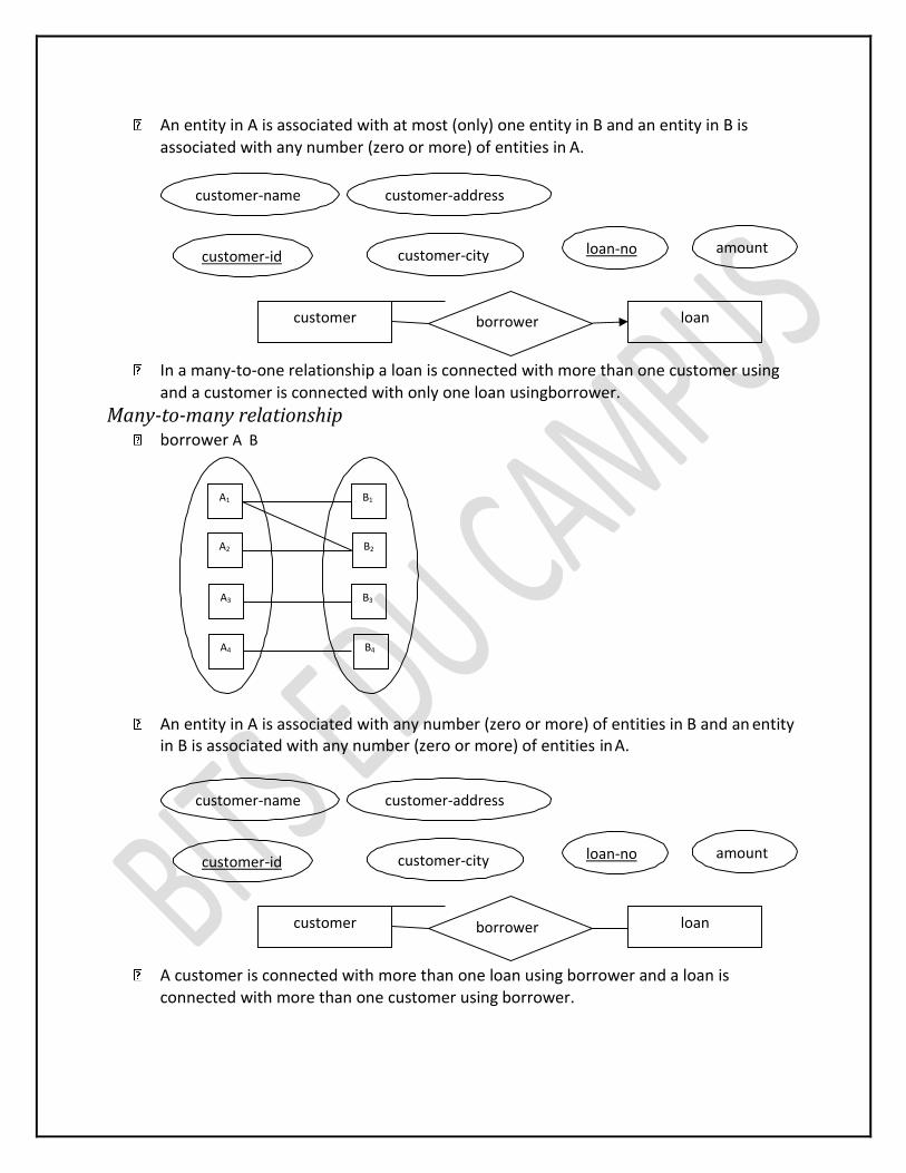
An entity in A is associated with at most (only) one entity in B and an entity in B is associated with any number (zero or more) of entities in A.
In a many-to-one relationship a loan is connected with more than one customer using and a customer is connected with only one loan usingborrower.
Many-to-many relationship borrower A B
An entity in A is associated with any number (zero or more) of entities in B and an entity in B is associated with any number (zero or more) of entities in A.
A customer is connected with more than one loan using borrower and a loan is connected with more than one customer using borrower.
customer-name customer-address
customer-id customer-city loan-no amount
borrower customer loan
A2 B2
A4 B4
A1 B1
A3 B3
customer-name customer-address
customer-id customer-city loan-no amount
borrower customer loan
payment-date
loan-no amount payment-no loan-amount
loan-payment payment loan
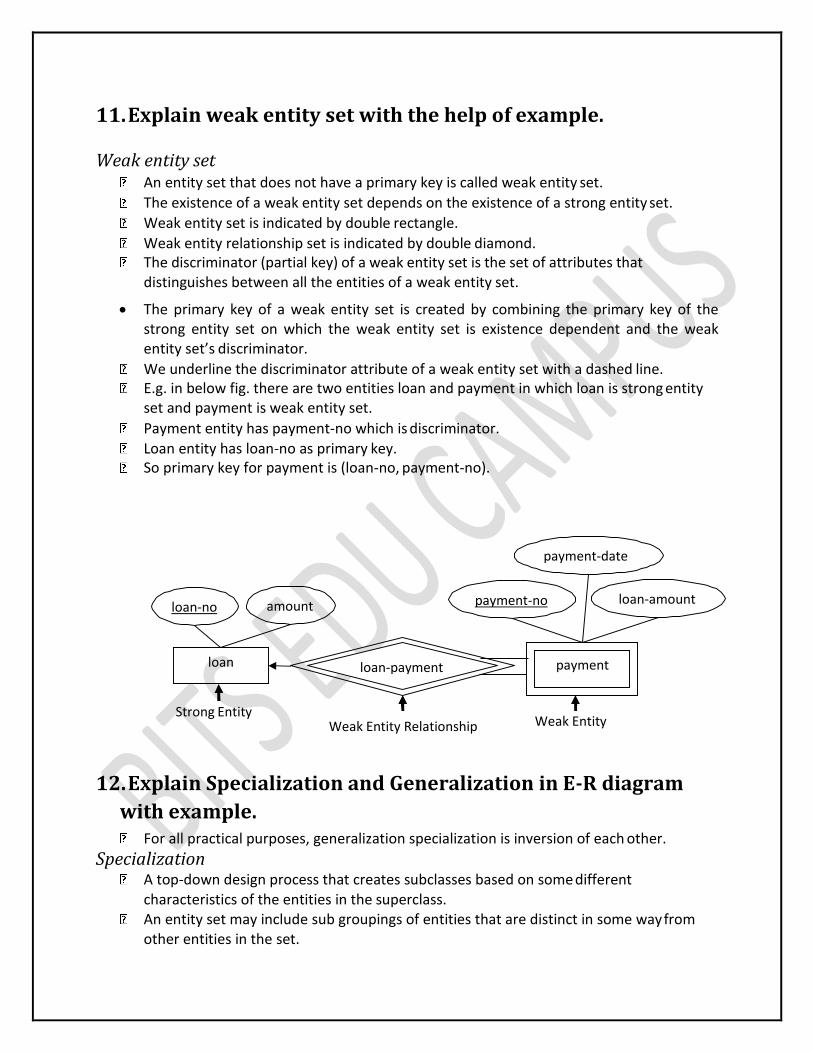
11. Explain weak entity set with the help of example. Weak entity set
An entity set that does not have a primary key is called weak entity set.
The existence of a weak entity set depends on the existence of a strong entity set.
Weak entity set is indicated by double rectangle.
Weak entity relationship set is indicated by double diamond. The discriminator (partial key) of a weak entity set is the set of attributes that
distinguishes between all the entities of a weak entity set.
The primary key of a weak entity set is created by combining the primary key of the strong entity set on which the weak entity set is existence dependent and the weak entity set’s discriminator.
We underline the discriminator attribute of a weak entity set with a dashed line. E.g. in below fig. there are two entities loan and payment in which loan is strong entity
set and payment is weak entity set.
Payment entity has payment-no which is discriminator.
Loan entity has loan-no as primary key. So primary key for payment is (loan-no, payment-no).
Strong Entity Weak Entity Relationship Weak Entity
12. Explain Specialization and Generalization in E-R diagram
with example. For all practical purposes, generalization specialization is inversion of each other.
Specialization A top-down design process that creates subclasses based on some different
characteristics of the entities in the superclass. An entity set may include sub groupings of entities that are distinct in some way from
other entities in the set.

For example, a subset of entities within an entity set may have attributes that are not shared by all the entities in the entity set.
Consider an entity set person, with attributes name, street and city.
A person may be further classified as one of the following:
customer
Employee
For example, customer entities may be described further by the attribute customer-id, credit-rating and employee entities may be described further by the attributes employee-id and salary.
The process of designating sub groupings within an entity set is called specialization. The specialization of person allows us to distinguish among persons according to whether they are employees or customers.
Now again, employees may be further classified as one of the following:
officer
teller
secretary Each of these employee types is described by a set of attributes that includes all the
attributes of entity set employee plus additional attributes. For example, officer entities may be described further by the attribute office-number,
tellerentities by the attributes station-number and hours-per-week, and secretary entities by the attribute hours-per-week.
In terms of an E-R diagram, specialization is depicted by a triangle component labeled ISA.
The label ISA stands for “is a” and represents, for example, that a customer “is a” person.
The ISA relationship may also be referred to as a superclass subclass relationship.
Generalization A bottom-up design process that combines number of entity sets that have same
features into a higher-level entity set. The design process proceed in a bottom-up manner, in which multiple entity sets are
synthesized into a higher level entity set on the basis of common features. The database designer may have to first identify a customer entity set with the
attributes name, street, city, and customer-id, and an employee entity set with the attributes name, street, city, employee-id, and salary.
But customer entity set and the employee entity set have some attributes common. This commonality can be expressed by generalization, which is a containment relationship that exists between a higher level entity set and one or more lower level entity sets.
In our example, person is the higher level entity set and customer and employee are lower level entity sets.
Higher level entity set is called superclass and lower level entity set is called subclass. So the person entity set is the superclass of two subclasses customer and employee.

Phone
13. Explain the steps to reduce the ER diagram to ER database schema.
Step 1: Entities and Simple Attributes:
An entity type within ER diagram is turned into a table. You may preferably keep the same name for the entity or give it a sensible name but avoid DBMS reserved words as well as avoid the use of special characters.
Each attribute turns into a column (attribute) in the table. The key attribute of the entity is the primary key of the table which is usually underlined. It can be composite if required but can never be null.
It is highly recommended that every table should start with its primary key attribute conventionally named as TablenameID.
Consider the following simple ER diagram:
The initial relational schema is expressed in the following format writing the table names with the attributes list inside a parentheses as shown below
Persons( personid, name, address, email ) Persons and Phones are Tables and personid, name, address and email are Columns
(Attributes). personid is the primary key for the table : Person
Step 2: Multi-Valued Attributes A multi-valued attribute is usually represented with a double-line oval.
PersonID Phone
Name Address Email
Person
PersonID Person
WifeID Name Wife
If you have a multi-valued attribute, take that multi-valued attribute and turn it into a new entity or table of its own.
Then make a 1:N relationship between the new entity and the existing one.
In simple words. 1. Create a table for that multi-valued attribute. 2. Add the primary (id) column of the parent entity as a foreign key within
the new table as shown below:
First table is Persons ( personid, name, lastname, email )
Second table is Phones ( phoneid , personid, phone )
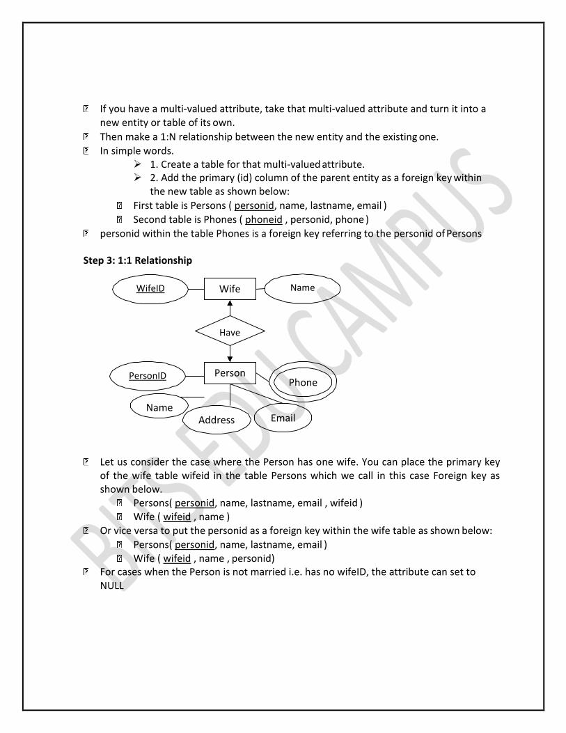
personid within the table Phones is a foreign key referring to the personid of Persons Step 3: 1:1 Relationship
Let us consider the case where the Person has one wife. You can place the primary key
of the wife table wifeid in the table Persons which we call in this case Foreign key as shown below.
Persons( personid, name, lastname, email , wifeid ) Wife ( wifeid , name )
Or vice versa to put the personid as a foreign key within the wife table as shown below:
Persons( personid, name, lastname, email ) Wife ( wifeid , name , personid)
For cases when the Person is not married i.e. has no wifeID, the attribute can set to NULL
Have
PersonID Phone
Name Address Email
Person
HouseID House
CountryID Name Country
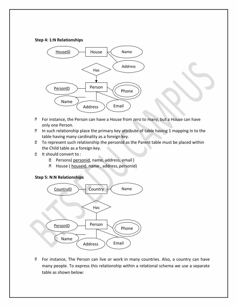
Step 4: 1:N Relationships
For instance, the Person can have a House from zero to many, but a House can have only one Person.
In such relationship place the primary key attribute of table having 1 mapping in to the table having many cardinality as a foreign key.
To represent such relationship the personid as the Parent table must be placed within the Child table as a foreign key.
It should convert to :
Persons( personid, name, address, email )
House ( houseid, name , address, personid) Step 5: N:N Relationships
For instance, The Person can live or work in many countries. Also, a country can have
many people. To express this relationship within a relational schema we use a separate
table as shown below:
Name
Address Has
PersonID Phone
Name Address Email
Person
Has
PersonID Phone
Name Address Email
Person
It should convert into :
Persons( personid, name, lastname, email ) Countries ( countryid, name, code) HasRelat ( hasrelatid, personid , countryid)
14. Define functional dependency. Explain different types of FD with the help of example. Explain the use of functional dependency in database design.
Functional Dependency
Let R be a relation schema having n attributes A1, A2, A3,…, An. Let attributes X and Y are two subsets of attributes of relation R. If the values of the X component of a tuple uniquely (or functionally) determine the
values of the Y component, then, there is a functional dependency from X to Y.
This is denoted by X → Y.
It is referred as: Y is functionally dependent on the X, or X functionally determines Y.
The abbreviation for functional dependency is FD or fd. The set of attributes X is called the left hand side of the FD, and Y is called the right hand
side. The left hand side of the FD is also referred as determinant whereas the right hand side
of the FD is referred as dependent.
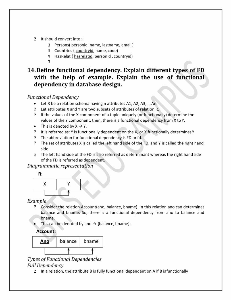
Diagrammatic representation
R:
Example Consider the relation Account(ano, balance, bname). In this relation ano can determines
balance and bname. So, there is a functional dependency from ano to balance and bname.
This can be denoted by ano → {balance, bname}.
Account:
Ano balance bname
Types of Functional Dependencies Full Dependency
In a relation, the attribute B is fully functional dependent on A if B is functionally
dependent on A, but not on any proper subset of A.
Eg. {Roll_No, Department_Name}→SPI
Partial Dependency In a relation, the attribute B is partial functional dependent on A if B is functionally
dependent on A as well as on any proper subset of A.
If there is some attribute that can be removed from A and the still dependency holds.
Eg. {Enrollment_No, Department_Name}→SPI
Transitive Dependency In a relation, if attribute(s) A→B and B→C, then C is transitively depends on A via B
(provided that A is not functionally dependent on B or C).
Eg. Staff_No→Branch_No and Branch_No→Branch_Address
Trivial FD: X→Y is trivial FDif Y is a subset of X
Eg.{Roll_No, Department_Name}→Roll_No
Nontrivial FD X→Y is nontrivial FDif Y is not a subset of X
Eg.. {Roll_No, Department_Name}→Student_Name
Use of functional dependency in database design To test relations to see if they are legal under a given set of functional dependencies. If a
relation r is legal under a set F of functional dependencies, we say that r satisfies F.
To specify constraints on the set of legal relations.
15. What is decomposition? Explain different types of
decomposition. Decomposition
Decomposition is the process of breaking down given relation into two or more relations.
Here, relation R is replaced by two or more relations in such a way that -1. Each new relation contains a subset of the attributes of R, and 2. Together, they all include all tuples and attributes of R.
Relational database design process starts with a universal relation schema R = {A1, A2, A3,..., An), which includes all the attributes of the database. The universal relation states that every attribute name is unique.
Using functional dependencies, this universal relation schema is decomposed into a set of relation schemas D = {R1, R2, R3,…,Rm}.
Now, D becomes the relational database schema and D is referred as decomposition of R.
Generally, decomposition is used to eliminate the pitfalls of the poor database design during normalization process.
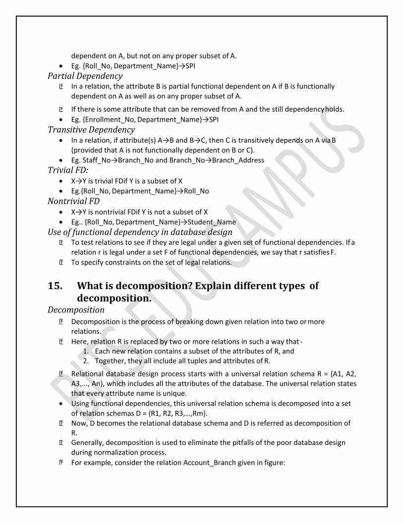
For example, consider the relation Account_Branch given in figure:
Account_Branch Ano Balance Bname Baddress
A01 5000 Vvn Mota bazaar, VVNagar A02 6000 Ksad Chhota bazaar, Karamsad A03 7000 Anand Nana bazaar, Anand
A04 8000 Ksad Chhota bazaar, Karamsad
A05 6000 Vvn Mota bazaar, VVNagar
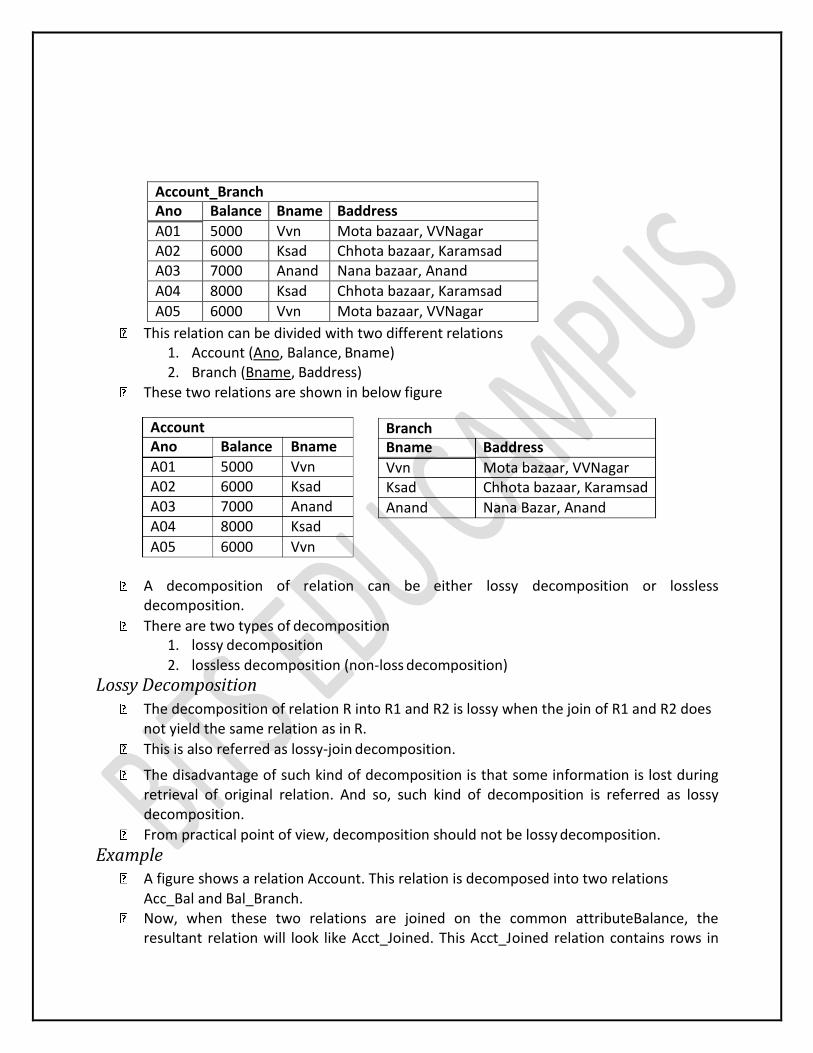
This relation can be divided with two different relations1. Account (Ano, Balance, Bname) 2. Branch (Bname, Baddress)
These two relations are shown in below figure
A decomposition of relation can be either lossy decomposition or lossless decomposition.
There are two types of decomposition1. lossy decomposition
2. lossless decomposition (non-loss decomposition)
Lossy Decomposition The decomposition of relation R into R1 and R2 is lossy when the join of R1 and R2 does
not yield the same relation as in R.
This is also referred as lossy-join decomposition.
The disadvantage of such kind of decomposition is that some information is lost during retrieval of original relation. And so, such kind of decomposition is referred as lossy decomposition.
From practical point of view, decomposition should not be lossy decomposition.
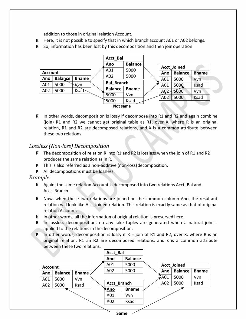
Example A figure shows a relation Account. This relation is decomposed into two relations
Acc_Bal and Bal_Branch. Now, when these two relations are joined on the common attributeBalance, the
resultant relation will look like Acct_Joined. This Acct_Joined relation contains rows in
Account Ano Balance Bname
A01 5000 Vvn A02 6000 Ksad A03 7000 Anand A04 8000 Ksad
A05 6000 Vvn
Branch Bname Baddress
Vvn Mota bazaar, VVNagar Ksad Chhota bazaar, Karamsad
Anand Nana Bazar, Anand
Same
addition to those in original relation Account.
Here, it is not possible to specify that in which branch account A01 or A02 belongs.
So, information has been lost by this decomposition and then join operation.
Not same
In other words, decomposition is lossy if decompose into R1 and R2 and again combine (join) R1 and R2 we cannot get original table as R1, over X, where R is an original relation, R1 and R2 are decomposed relations, and X is a common attribute between these two relations.
Lossless (Non-loss) Decomposition The decomposition of relation R into R1 and R2 is lossless when the join of R1 and R2
produces the same relation as in R.
This is also referred as a non-additive (non-loss) decomposition.
All decompositions must be lossless.
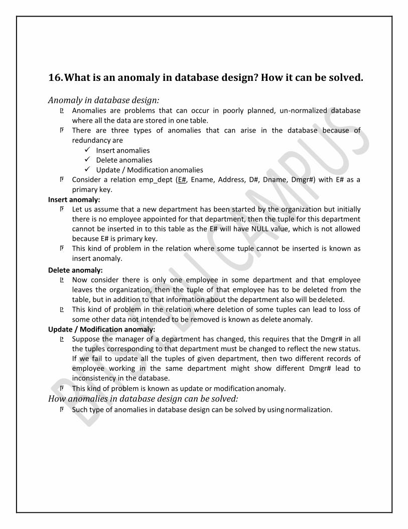
Example Again, the same relation Account is decomposed into two relations Acct_Bal and
Acct_Branch.
Now, when these two relations are joined on the common column Ano, the resultant relation will look like Acc_Joined relation. This relation is exactly same as that of original relation Account.
In other words, all the information of original relation is preserved here. In lossless decomposition, no any fake tuples are generated when a natural join is
applied to the relations in the decomposition. In other words, decomposition is lossy if R = join of R1 and R2, over X, where R is an
original relation, R1 an R2 are decomposed relations, and x is a common attribute between these two relations.
Acct_Bal Ano Balance A01 5000 A02 5000
Acct_Joined Ano Balance Bname
A01 5000 Vvn A01 5000 Ksad
A02 5000 Vvn
A02 5000 Ksad
Account Ano Balance Bname
A01 5000 Vvn A02 5000 Ksad
Bal_Branch Balance Bname 5000 Vvn 5000 Ksad
Acct_Bal Ano Balance A01 5000 A02 5000
Acct_Joined Ano Balance Bname
A01 5000 Vvn A02 5000 Ksad
Account Ano Balance Bname
A01 5000 Vvn A02 5000 Ksad
Acct_Branch Ano Bname
A01 Vvn
A02 Ksad
16. What is an anomaly in database design? How it can be solved. Anomaly in database design:
Anomalies are problems that can occur in poorly planned, un-normalized database where all the data are stored in one table.
There are three types of anomalies that can arise in the database because of redundancy are
Insert anomalies Delete anomalies Update / Modification anomalies
Consider a relation emp_dept (E#, Ename, Address, D#, Dname, Dmgr#) with E# as a primary key.
Insert anomaly: Let us assume that a new department has been started by the organization but initially
there is no employee appointed for that department, then the tuple for this department cannot be inserted in to this table as the E# will have NULL value, which is not allowed because E# is primary key.
This kind of problem in the relation where some tuple cannot be inserted is known as insert anomaly.
Delete anomaly: Now consider there is only one employee in some department and that employee
leaves the organization, then the tuple of that employee has to be deleted from the table, but in addition to that information about the department also will be deleted.
This kind of problem in the relation where deletion of some tuples can lead to loss of some other data not intended to be removed is known as delete anomaly.
Update / Modification anomaly: Suppose the manager of a department has changed, this requires that the Dmgr# in all
the tuples corresponding to that department must be changed to reflect the new status. If we fail to update all the tuples of given department, then two different records of employee working in the same department might show different Dmgr# lead to inconsistency in the database.
This kind of problem is known as update or modification anomaly.
How anomalies in database design can be solved: Such type of anomalies in database design can be solved by using normalization.
17. What is normalization? What is the need of it?
OR What is normalization? Why normalization process is needed?
OR Explain different types of normal forms with example. OR
Explain 1NF, 2NF, 3NF, BCNF, 4NF and 5NF with example. Normalization
Database normalization is the process of removing redundant data from your tables to improve storage efficiency, data integrity, and scalability.
In the relational model, methods exist for quantifying how efficient a database is. These classifications are called normal forms (or NF), and there are algorithms for converting a given database between them.
Normalization generally involves splitting existing tables into multiple ones, which must be re-joined or linked each time a query is issued.
Need of Normalization Eliminates redundant data Reduces chances of data errors
Reduces disk space Improve data integrity, scalability and data consistency.
1NF
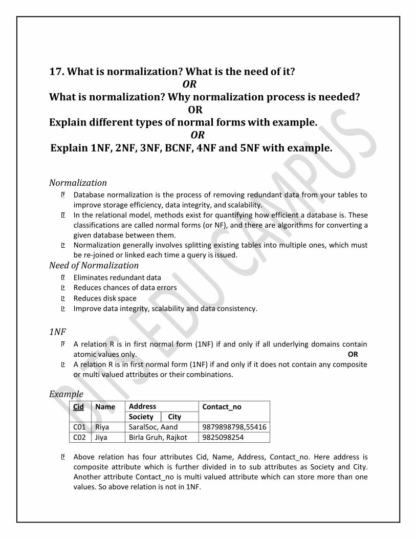
A relation R is in first normal form (1NF) if and only if all underlying domains contain atomic values only. OR
A relation R is in first normal form (1NF) if and only if it does not contain any composite or multi valued attributes or their combinations.
Example
Cid Name Address Contact_no Society City
C01 Riya SaralSoc, Aand 9879898798,55416
C02 Jiya Birla Gruh, Rajkot 9825098254
Above relation has four attributes Cid, Name, Address, Contact_no. Here address is composite attribute which is further divided in to sub attributes as Society and City. Another attribute Contact_no is multi valued attribute which can store more than one values. So above relation is not in 1NF.
Problem Suppose we want to find all customers for some particular city then it is difficult to
retrieve. Reason is city name is combined with society name and stored whole as address.
Solution
Insert separate attribute for each sub attribute of composite attribute. Insert separate attribute for multi valued attribute and insert only one value on one
attribute and other in other attribute.
So above table can be created as follows.
Cid Name Society City Contact_no1 Contact_no2
C01 Riya SaralSoc Aand 9879898798 55416 C02 Jiya Birla Gruh Rajkot 9825098254
2NF A relation R is in second normal form (2NF) if and only if it is in 1NF and every non-key
attribute is fully dependent on the primary key. OR A relation R is in second normal form (2NF) if and only if it is in 1NF and no any non-key
attribute is partially dependent on the primary key.
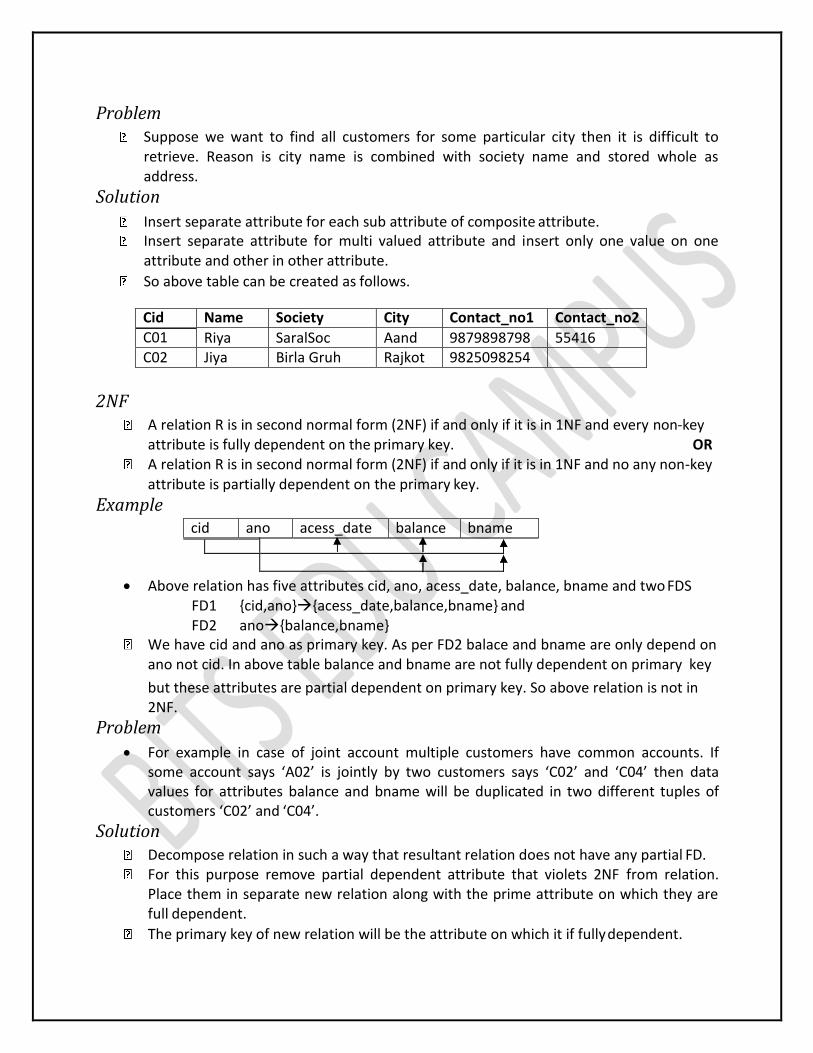
Example cid ano acess_date balance bname
Above relation has five attributes cid, ano, acess_date, balance, bname and two FDS FD1 {cid,ano}{acess_date,balance,bname} andFD2 ano{balance,bname}
We have cid and ano as primary key. As per FD2 balace and bname are only depend on ano not cid. In above table balance and bname are not fully dependent on primary key
but these attributes are partial dependent on primary key. So above relation is not in 2NF.
Problem
For example in case of joint account multiple customers have common accounts. If some account says ‘A02’ is jointly by two customers says ‘C02’ and ‘C04’ then data values for attributes balance and bname will be duplicated in two different tuples of customers ‘C02’ and ‘C04’.
Solution Decompose relation in such a way that resultant relation does not have any partial FD. For this purpose remove partial dependent attribute that violets 2NF from relation.
Place them in separate new relation along with the prime attribute on which they are full dependent.
The primary key of new relation will be the attribute on which it if fully dependent.
Keep other attribute same as in that table with same primary key.
So above table can be decomposed as per following.
ano balance bname
cid ano acess_date
3NF A relation R is in third normal form (3NF) if and only if it is in 2NF and every non-key
attribute is non-transitively dependent on the primary key.
An attribute C is transitively dependent on attribute A if there exist an attribute B such that: A B and B C.
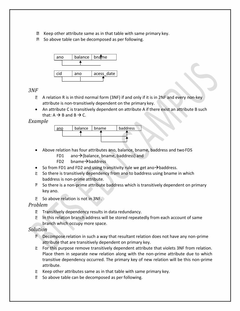
Example
Above relation has four attributes ano, balance, bname, baddress and two FDS FD1 ano{balance, bname, baddress} andFD2 bnamebaddress
So from FD1 and FD2 and using transitivity rule we get anobaddress. So there is transitively dependency from ano to baddress using bname in which
baddress is non-prime attribute. So there is a non-prime attribute baddress which is transitively dependent on primary
key ano.
So above relation is not in 3NF.
Problem Transitively dependency results in data redundancy. In this relation branch address will be stored repeatedly from each account of same
branch which occupy more space.
Solution Decompose relation in such a way that resultant relation does not have any non-prime
attribute that are transitively dependent on primary key. For this purpose remove transitively dependent attribute that violets 3NF from relation.
Place them in separate new relation along with the non-prime attribute due to which transitive dependency occurred. The primary key of new relation will be this non-prime attribute.
Keep other attributes same as in that table with same primary key.
So above table can be decomposed as per following.
ano balance bname baddress
ano balance bname
bname baddress
BCNF A relation R is in BCNF if and only if it is in 3NF and no any prime attribute is transitively
dependent on the primary key. An attribute C is transitively dependent on attribute A if there exist an attribute B such
that AB and BC.
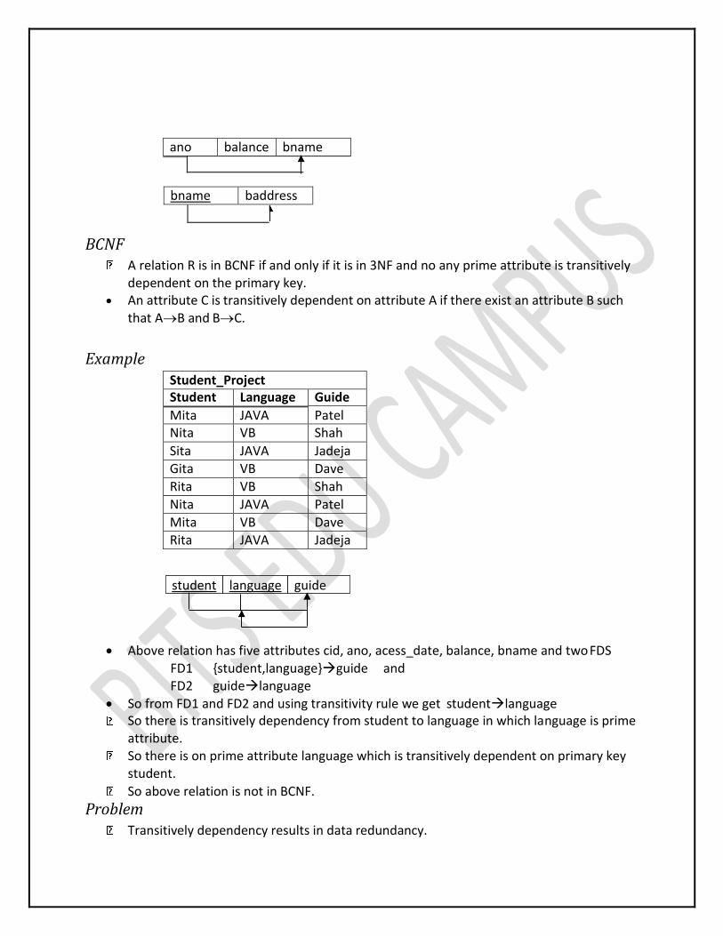
Example
Student_Project Student Language Guide
Mita JAVA Patel Nita VB Shah
Sita JAVA Jadeja Gita VB Dave
Rita VB Shah
Nita JAVA Patel
Mita VB Dave Rita JAVA Jadeja
Above relation has five attributes cid, ano, acess_date, balance, bname and two FDS FD1 {student,language}guide andFD2 guidelanguage
So from FD1 and FD2 and using transitivity rule we get studentlanguage So there is transitively dependency from student to language in which language is prime
attribute. So there is on prime attribute language which is transitively dependent on primary key
student.
So above relation is not in BCNF.
Problem Transitively dependency results in data redundancy.
student language guide
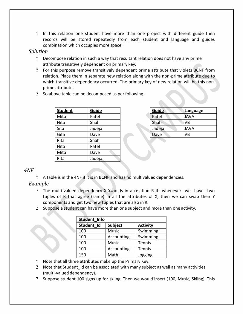
In this relation one student have more than one project with different guide then records will be stored repeatedly from each student and language and guides combination which occupies more space.
Solution Decompose relation in such a way that resultant relation does not have any prime
attribute transitively dependent on primary key. For this purpose remove transitively dependent prime attribute that violets BCNF from
relation. Place them in separate new relation along with the non-prime attribute due to which transitive dependency occurred. The primary key of new relation will be this non- prime attribute.
So above table can be decomposed as per following.
4NF A table is in the 4NF if it is in BCNF and has no multivalued dependencies.
Example The multi-valued dependency X Y holds in a relation R if whenever we have two
tuples of R that agree (same) in all the attributes of X, then we can swap their Y components and get two new tuples that are also in R.
Suppose a student can have more than one subject and more than one activity.
Student_Info Student_Id Subject Activity 100 Music Swimming 100 Accounting Swimming
100 Music Tennis
100 Accounting Tennis
150 Math Jogging
Note that all three attributes make up the Primary Key. Note that Student_Id can be associated with many subject as well as many activities
(multi-valued dependency). Suppose student 100 signs up for skiing. Then we would insert (100, Music, Skiing). This
Student Guide
Mita Patel Nita Shah
Sita Jadeja
Gita Dave Rita Shah
Nita Patel
Mita Dave
Rita Jadeja
Guide Language
Patel JAVA Shah VB
Jadeja JAVA
Dave VB
row implies that student 100 skies as Music subject but not as an accounting subject, so in order to keep the data consistent we must add one more row (100, Accounting, Skiing). This is an insertion anomaly.
Suppose we have a relation R(A) with a multivalued dependency X Y. The MVD can be removed by decomposing R into R1(R - Y) and R2(X U Y).
Here are the tables Normalized
5NF A table is in the 5NF if it is in 4NF and if for all Join dependency (JD) of (R1, R2, R3, ...,Rm)
in R, every Ri is a superkey for R. OR A table is in the 5NF if it is in 4NF and if it cannot have a lossless decomposition in to any
number of smaller tables (relations). It is also known as Project-join normal form (PJ/NF).
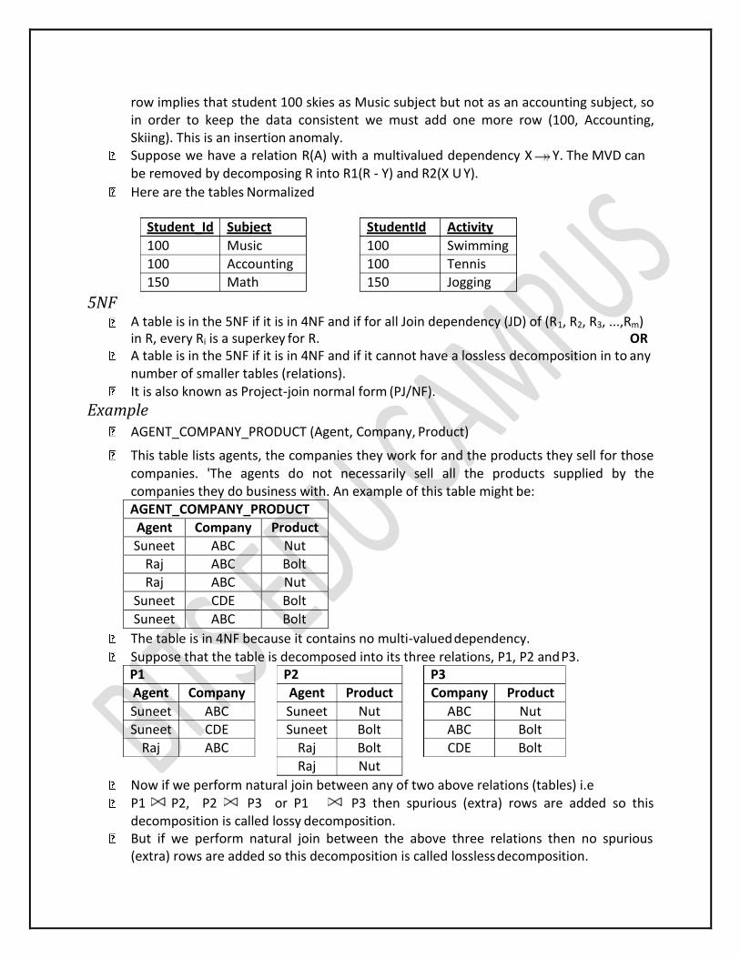
Example AGENT_COMPANY_PRODUCT (Agent, Company, Product)
This table lists agents, the companies they work for and the products they sell for those companies. 'The agents do not necessarily sell all the products supplied by the companies they do business with. An example of this table might be:AGENT_COMPANY_PRODUCT
Agent Company Product
Suneet ABC Nut Raj ABC Bolt
Raj ABC Nut
Suneet CDE Bolt
Suneet ABC Bolt
The table is in 4NF because it contains no multi-valued dependency.
Suppose that the table is decomposed into its three relations, P1, P2 and P3.
Now if we perform natural join between any of two above relations (tables) i.e P1 P2, P2 P3 or P1 P3 then spurious (extra) rows are added so this
decomposition is called lossy decomposition. But if we perform natural join between the above three relations then no spurious
(extra) rows are added so this decomposition is called lossless decomposition.
P1
Agent Company
Suneet ABC Suneet CDE
Raj ABC
P2
Agent Product
Suneet Nut Suneet Bolt
Raj Bolt
Raj Nut
P3
Company Product
ABC Nut ABC Bolt
CDE Bolt
Student_Id Subject
100 Music
100 Accounting
150 Math
StudentId Activity
100 Swimming
100 Tennis
150 Jogging
So above three tables P1, P2 and P3 are in 5 NF.
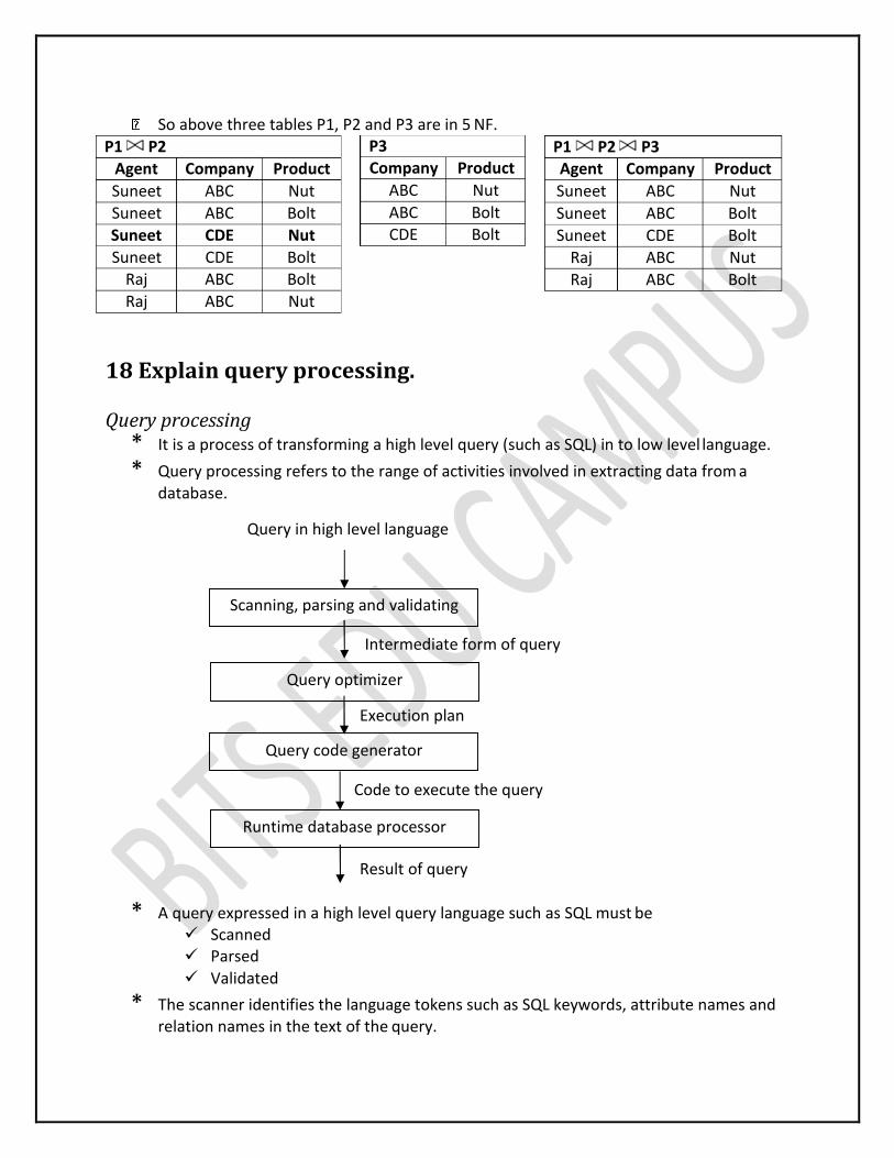
18 Explain query processing. Query processing
* It is a process of transforming a high level query (such as SQL) in to low level language.
* Query processing refers to the range of activities involved in extracting data from a database.
Query in high level language
Intermediate form of query
Execution plan
Code to execute the query
Result of query
* A query expressed in a high level query language such as SQL must be Scanned Parsed
Validated
* The scanner identifies the language tokens such as SQL keywords, attribute names and relation names in the text of the query.
P1 P2
Agent Company Product
Suneet ABC Nut
Suneet ABC Bolt
Suneet CDE Nut
Suneet CDE Bolt Raj ABC Bolt
Raj ABC Nut
P3 Company Product
ABC Nut
ABC Bolt CDE Bolt
P1 P2 P3 Agent Company Product
Suneet ABC Nut
Suneet ABC Bolt
Suneet CDE Bolt
Raj ABC Nut
Raj ABC Bolt
Query optimizer
Runtime database processor
Scanning, parsing and validating
Query code generator
* Parser checks the query syntax to determine whether it is formulated according to the syntax rules of the query language.
* The query must also be validated by checking that all attributes and relation names are valid and semantically meaningful names in the schema of the particular database being queried.
* A query typically has many possible execution strategies and the process of choosing a suitable one for processing a query is known as query optimization.
* The query optimizer module has the task of producing an execution plan and code generator generates the code to execute that plan.
* The runtime database processor has the task of running the query code whether in compiled or interpreted mode, to produce the query result.
* If a runtime error results, an error message is generated by the runtime database processor.
* Query code generator will generate code for query.* Runtime database processor will select optimal plan and execute query and gives result.
19.Explain various steps involved in query evaluation. OR Explain query evaluation process. OR Explain evaluation expression process in query optimization.
* There are two methods for the evaluation of expression1. Materialization 2. Pipelining
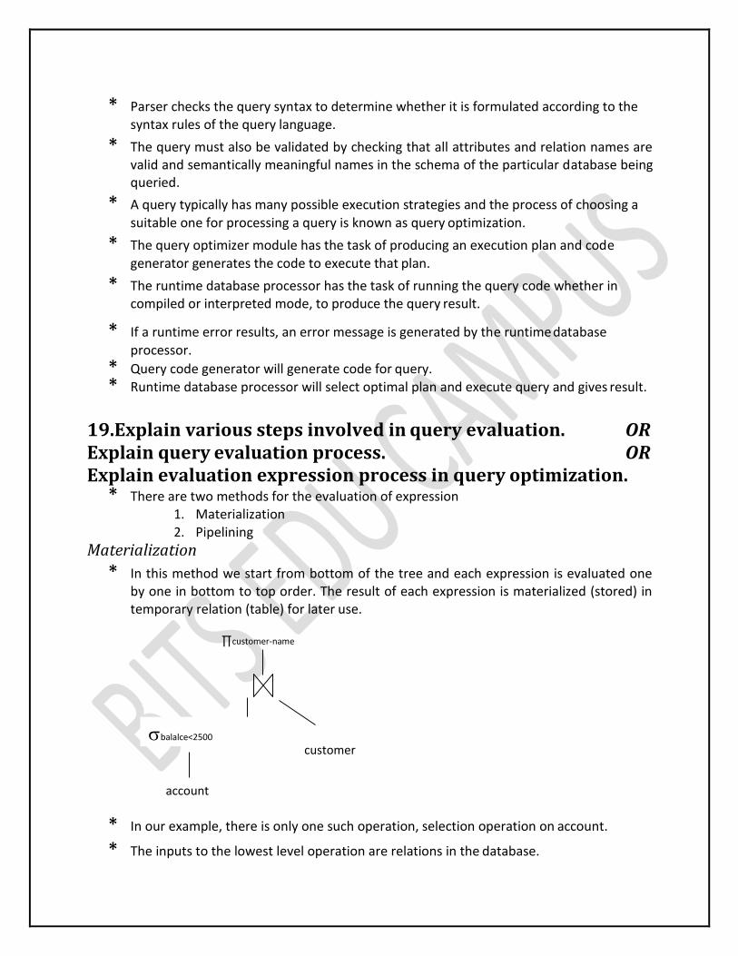
Materialization
* In this method we start from bottom of the tree and each expression is evaluated one by one in bottom to top order. The result of each expression is materialized (stored) in temporary relation (table) for later use.
∏customer-name
customer
account
* In our example, there is only one such operation, selection operation on account.
* The inputs to the lowest level operation are relations in the database.
balalce<2500
* We execute these operations and we store the results in temporary relations.
* We can use these temporary relations to execute the operation at the next level up in the tree, where the inputs now are either temporary relations or relations stored in the database.
* In our example the inputs to join are the customer relation and the temporary relation created by the selection on account.
* The join can now be evaluated, creating another temporary relation.
* By repeating the process, we will finally evaluate the operation at the root of the tree, giving the final result of the expression.
* In our example, we get the final result by executing the projection operation at the root of the tree, using as input the temporary relation created by the join. Evaluation just described is called materialized evaluation, since the results of each intermediate operation are created and then are used for evaluation of the next level operations.
* The cost of a materialized evaluation is not simply the sum of the costs of the operations involved. To compute the cost of evaluating an expression is to add the cost of all the operation as well as the cost of writing intermediate results to disk.
* The disadvantage of this method is that it will create temporary relation (table) and that relation is stored on disk which consumes space on disk.
* It evaluates one operation at a time, starting at the lowest level.
Pipelining
* We can reduce the number of temporary files that are produced by combining several relations operations into pipeline operations, in which the results of one operation are passed along to the next operation in the pipeline. Combining operations into a pipeline eliminates the cost reading and writing temporary relations.
* In this method several expression are evaluated simultaneously in pipeline by using the result of one operation passed to next without storing it in a temporary relation.
* First it will compute records having balance less than 2500 and then pass this result directly to project without storing that result in any temporary relation (table). And then by using this result it will compute the projections on customer-name.
* It is much cheaper than materialization because in this method no need to store a temporary relation to disk.
* Pipelining is not used in sort, hash joins.
20 Explain the measures of query cost, selection operation and join. OR Explain the measures of finding out the cost of a query in query processing. Measures of query cost
* The cost of query evaluation can be measured in terms of a number of different
resources including disk access, CPU time to execute a query and in a distributed or
parallel database system the cost of communication.
* The response time for a query evaluation plan i.e the time required to execute the plan
(assuming no other activity is going on) on the computer would account for all these
activities.
* In large database system, however disk accesses are usually the most important cost,
since disk access are slow compared to in memory operation.
* Moreover, CPU speeds have been improving much faster than have a disk speed.
* Therefore it is likely that the time spent in disk activity will continue to dominate the
total time to execute a query.
* Estimating the CPU time is relatively hard, compared to estimating disk access cost.
* Therefore disk access cost a reasonable measure of the cost of a query evaluation plan.
* Disk access is the predominant cost (in terms of time) relatively easy to estimate;
therefore number of block transfers from/to disk is typically used as measures.
* We use the number of block transfers from disk as a measure of actual cost.
* To simplify our computation, we assume that all transfer of blocks have same cost.
* To get more precise numbers we need to distinguish between sequential I/O where
blocks read are contiguous on disk and random I/O where blocks are non-contiguous
and an extra seek cost must be paid for each disk I/O operations.
* We also need to distinguish between read and write of blocks since it takes more time
to write a block on disk than to read a block from disk.
21 What is transaction? List and explain ACID property of transaction with example. Transaction
* A transaction is a part of program execution that accesses and updates various data items.
* A transaction can be defined as a group of tasks in which a single task is the minimum processing unit of work, which cannot be divided further.
* A transaction is a logical unit of work that contains one or more SQL statements.
* A transaction is an atomic unit (transaction either complete 0% or 100%).
* A database transaction must be atomic, meaning that it must be either entirely completed or aborted.
ACID property Atomicity
* Either all operations of the transaction are properly reflected in the database or none are.
* Means either all the operations of a transaction are executed or not a single operation is executed.
* For example consider below transaction to transfer Rs. 50 from account A to account B:1. read(A) 2. A := A – 50 3. write(A) 4. read(B) 5. B := B + 50
6. write(B)
* In above transaction if Rs. 50 is deducted from account A then it must be added to account B.
Consistency * Execution of a transaction in isolation preserves the consistency of the database.
* Means our database must remain in consistent state after execution of any transaction.
* In above example total of A and B must remain same before and after the execution of transaction.
Isolation
* Although multiple transactions may execute concurrently, each transaction must be unaware of other concurrently executing transactions.
* Intermediate transaction results must be hidden from other concurrently executed transactions.
* In above example once your transaction start from step one its result should not be
access by any other transaction until last step (step 6) is completed.
Durability
* After a transaction completes successfully, the changes it has made to the database persist, even if there are system failures.
* Once your transaction completed up to step 6 its result must be stored permanently. It should not be removed if system fails.
22.Explain different states in transaction processing in database. OR Explain State Transition Diagram (Transaction State Diagram).
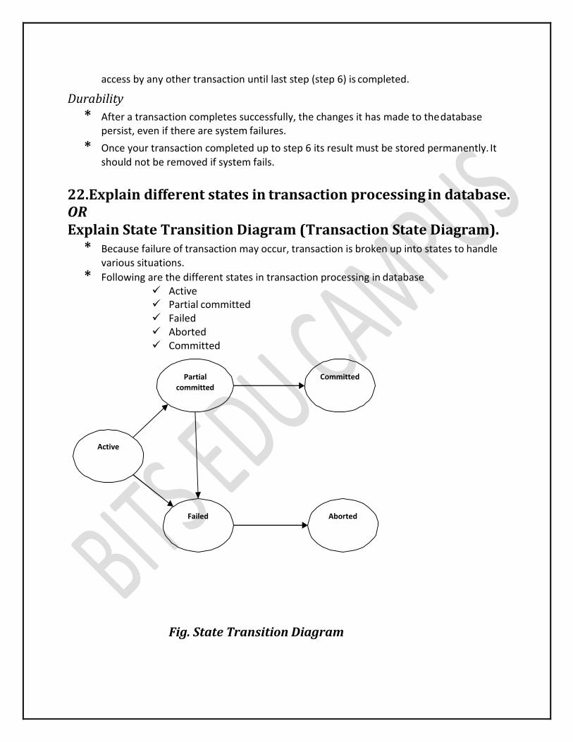
* Because failure of transaction may occur, transaction is broken up into states to handle various situations.
* Following are the different states in transaction processing in database Active Partial committed Failed Aborted Committed
Fig. State Transition Diagram
Partial
committed
Committed
Active
Failed Aborted

Active * This is the initial state. The transaction stays in this state while it is executing.
Partially Committed * This is the state after the final statement of the transaction is executed.
* At this point failure is still possible since changes may have been only done in main memory, a hardware failure could still occur.
* The DBMS needs to write out enough information to disk so that, in case of a failure, the system could re-create the updates performed by the transaction once the system is brought back up.
* After it has written out all the necessary information, it is committed.
Failed
* After the discovery that normal execution can no longer proceed.
* Once a transaction cannot be completed, any changes that it made must be undone rolling it back.
Aborted
* The state after the transaction has been rolled back and the database has been restored to its state prior to the start of the transaction.
Committed * The transaction enters in this state after successful completion of the transaction.
* We cannot abort or rollback a committed transaction.
23. Explain serializability of transaction. OR Explain both the forms of serializability with example. Also explain relation between two forms. OR Explain conflict serializability and view serializability with example. Conflict serializability
* Instructions li and lj of transactions Ti and Tj respectively, conflict if and only if there exists some item Q accessed by both li and lj, and at least one of these instructions wrote Q.
1. If li and lj access different data item then li and lj don’t conflict. 2. li = read(Q), lj = read(Q). li and lj don’t conflict. 3. li = read(Q), lj = write(Q). li and lj conflict. 4. li = write(Q), lj = read(Q). li and lj conflict. 5. li = write(Q), lj = write(Q). li and lj conflict.
* Intuitively, a conflict between li and lj forces a (logical) temporal order between them.
* If a schedule S can be transformed into a schedule S´ by a series of swaps of non- conflicting instructions, we say that S and S´ are conflict equivalent.
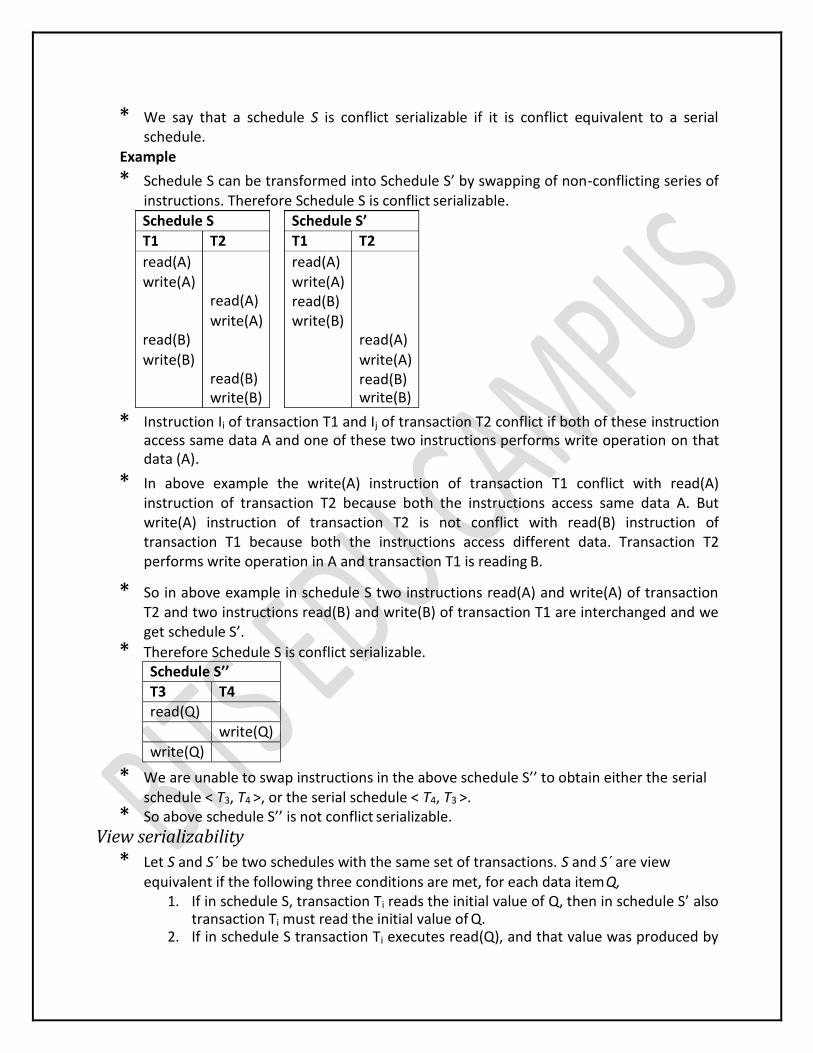
* We say that a schedule S is conflict serializable if it is conflict equivalent to a serial schedule.
Example
* Schedule S can be transformed into Schedule S’ by swapping of non-conflicting series of instructions. Therefore Schedule S is conflict serializable.
* Instruction Ii of transaction T1 and Ij of transaction T2 conflict if both of these instruction access same data A and one of these two instructions performs write operation on that data (A).
* In above example the write(A) instruction of transaction T1 conflict with read(A) instruction of transaction T2 because both the instructions access same data A. But write(A) instruction of transaction T2 is not conflict with read(B) instruction of transaction T1 because both the instructions access different data. Transaction T2 performs write operation in A and transaction T1 is reading B.
* So in above example in schedule S two instructions read(A) and write(A) of transaction T2 and two instructions read(B) and write(B) of transaction T1 are interchanged and we get schedule S’.
* Therefore Schedule S is conflict serializable.Schedule S’’
T3 T4 read(Q)
write(Q)
write(Q)
* We are unable to swap instructions in the above schedule S’’ to obtain either the serial
schedule < T3, T4 >, or the serial schedule < T4, T3 >.* So above schedule S’’ is not conflict serializable.
View serializability
* Let S and S´ be two schedules with the same set of transactions. S and S´ are view equivalent if the following three conditions are met, for each data item Q,
1. If in schedule S, transaction Ti reads the initial value of Q, then in schedule S’ also transaction Ti must read the initial value of Q.
2. If in schedule S transaction Ti executes read(Q), and that value was produced by
Schedule S
T1 T2
read(A)
write(A)
read(A)
read(B) write(A)
write(B)
read(B) write(B)
Schedule S’
T1 T2
read(A)
write(A)
read(B)
write(B)
read(A) write(A) read(B) write(B)

transaction Tj (if any), then in schedule S’ also transaction Ti must read the value of Q that was produced by the same write(Q) operation of transaction Tj .
3. The transaction Ti (if any) that performs the final write(Q) operation in schedule S then in schedule S’ also the final write(Q) operation must be performed by Ti.
* A schedule S is view serializable if it is view equivalent to a serial schedule.
* Every conflict serializable schedule is also view serializable but every view serializable is not conflict serializable.
* Below is a schedule which is view serializable but not conflict serializable.
Schedule S T3 T4 T6
read(Q)
write(Q)
write(Q)
write(Q)
* Above schedule is view serializable but not conflict serializable because all the transactions can use same data item (Q) and all the operations are conflict with each other due to one operation is write on data item (Q) and that’s why we cannot interchange any non conflict operation of any transaction.
24.Explain two phase commit protocol. OR Explain working of two phase commit protocol. Two phase commit protocol
• The two phase commit protocol provides an automatic recovery mechanism in case a system or media failure occurs during execution of the transaction.
• The two phase commit protocol ensures that all participants perform the same action (either to commit or to roll back a transaction).
• The two phase commit strategy is designed to ensure that either all the databases are updated or none of them, so that the databases remain synchronized.
• In two phase commit protocol there is one node which is act as a coordinator and all other participating node are known as cohorts or participant.
• Coordinator – the component that coordinates with all the participants. • Cohorts (Participants) – each individual node except coordinator are participant. • As the name suggests, the two phase commit protocol involves two phases.
1. The first phase is Commit Request phase OR phase 1 2. The second phase is Commit phase OR phase 2
Commit Request Phase (Obtaining Decision)
* To commit the transaction, the coordinator sends a request asking for “ready for commit” to each cohort.
* The coordinator waits until it has received a reply from all cohorts to “vote” on the request.
* Each participant votes by sending a message back to the coordinator as follows:
It votes YES if it is prepared to commit It may vote NO for any reason if it cannot prepare the transaction due to a local
failure. It may delay in voting because cohort was busy with other work.
Commit Phase (Performing Decision)
* If the coordinator receives YES response from all cohorts, it decides to commit. The transaction is now officially committed. Otherwise, it either receives a NO response or gives up waiting for some cohort, so it decides to abort.
* The coordinator sends its decision to all participants (i.e. COMMIT or ABORT).
* Participants acknowledge receipt of commit or about by replying DONE.
25. Explain Log based recovery method. Log based recovery
* The most widely used structure for recording database modification is the log.
* The log is a sequence of log records, recording all the update activities in the database.
* In short Transaction log is a journal or simply a data file, which contains history of all transaction performed and maintained on stable storage.
* Since the log contains a complete record of all database activity, the volume of data stored in the log may become unreasonable large.
* For log records to be useful for recovery from system and disk failures, the log must reside on stable storage.
* Log contains1. Start of transaction 2. Transaction-id 3. Record-id 4. Type of operation (insert, update, delete) 5. Old value, new value
6. End of transaction that is committed or aborted. * All such files are maintained by DBMS itself. Normally these are sequential files.
* Recovery has two factors Rollback (Undo) and Roll forward (Redo).
* When transaction Ti starts, it registers itself by writing a <Ti start>log record
* Before Ti executes write(X), a log record <Ti, X, V1, V2> is written, where V1 is the value of X before the write, and V2 is the value to be written to X.
Log record notes that Ti has performed a write on data item Xj Xj had value V1 before the write, and will have value V2 after the write.
* When Ti finishes it last statement, the log record <Ti commit> is written.* Two approaches are used in log based recovery
1. Deferred database modification 2. Immediate database modification
Log based Recovery Techniques
* Once a failure occurs, DBMS retrieves the database using the back-up of database and
transaction log. Various log based recovery techniques used by DBMS are as per below:1. Deferred Database Modification 2. Immediate Database Modification
* Both of the techniques use transaction logs. Thesetechniques are explained in following sub-sections.
26 What are the three problems due to concurrency? How the problems can be avoided. Three problems due to concurrency
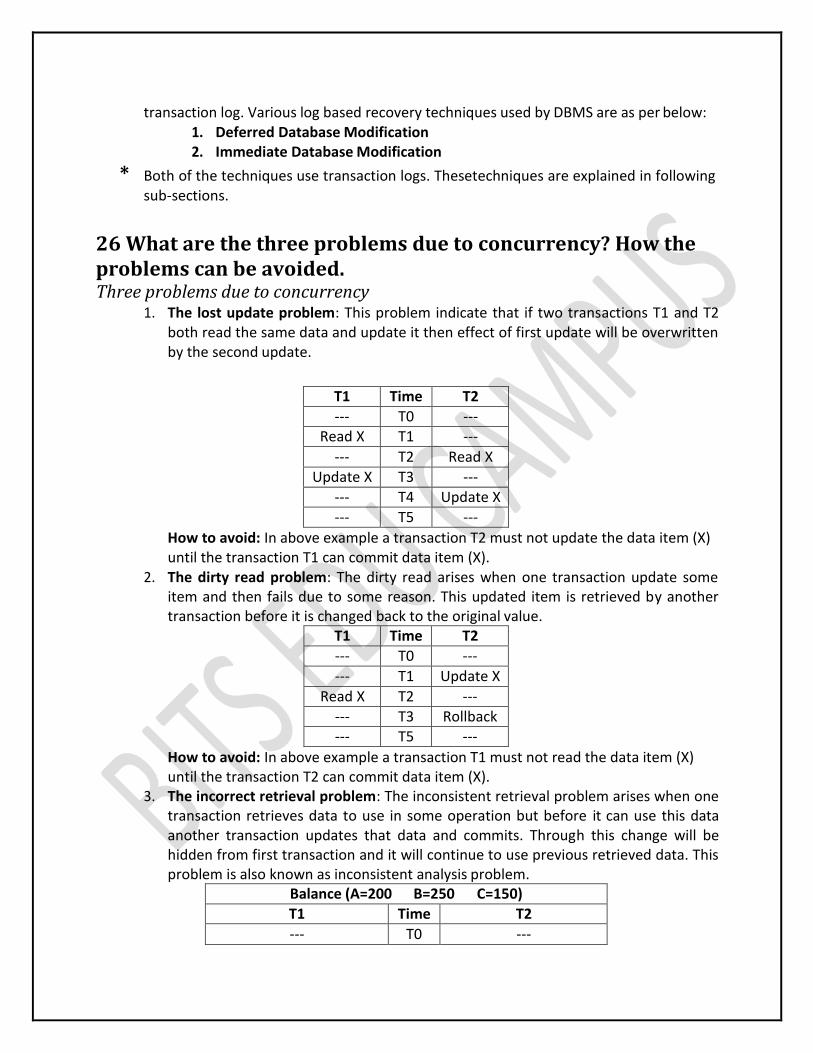
1. The lost update problem: This problem indicate that if two transactions T1 and T2 both read the same data and update it then effect of first update will be overwritten by the second update.
T1 Time T2
--- T0 --- Read X T1 ---
--- T2 Read X
Update X T3 ---
--- T4 Update X
--- T5 ---
How to avoid: In above example a transaction T2 must not update the data item (X) until the transaction T1 can commit data item (X).
2. The dirty read problem: The dirty read arises when one transaction update some item and then fails due to some reason. This updated item is retrieved by another transaction before it is changed back to the original value.
T1 Time T2
--- T0 ---
--- T1 Update X
Read X T2 ---
--- T3 Rollback --- T5 ---
How to avoid: In above example a transaction T1 must not read the data item (X) until the transaction T2 can commit data item (X).
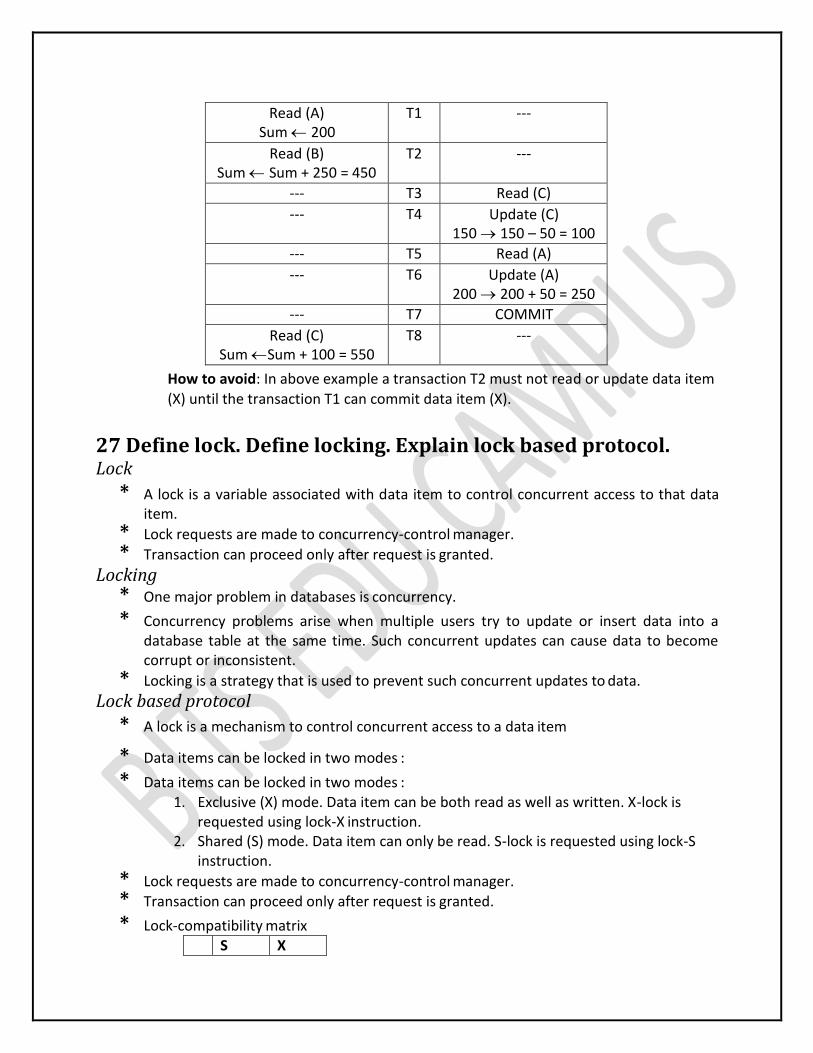
3. The incorrect retrieval problem: The inconsistent retrieval problem arises when one transaction retrieves data to use in some operation but before it can use this data another transaction updates that data and commits. Through this change will be hidden from first transaction and it will continue to use previous retrieved data. This problem is also known as inconsistent analysis problem.
Balance (A=200 B=250 C=150)
T1 Time T2
--- T0 ---
Read (A) Sum 200
T1 ---
Read (B) Sum Sum + 250 = 450
T2 ---
--- T3 Read (C)
--- T4 Update (C) 150 150 – 50 = 100
--- T5 Read (A)
--- T6 Update (A) 200 200 + 50 = 250
--- T7 COMMIT
Read (C) Sum Sum + 100 = 550
T8 ---
How to avoid: In above example a transaction T2 must not read or update data item
(X) until the transaction T1 can commit data item (X).
27 Define lock. Define locking. Explain lock based protocol. Lock
* A lock is a variable associated with data item to control concurrent access to that data item.
* Lock requests are made to concurrency-control manager.
* Transaction can proceed only after request is granted.
Locking * One major problem in databases is concurrency.
* Concurrency problems arise when multiple users try to update or insert data into a database table at the same time. Such concurrent updates can cause data to become corrupt or inconsistent.
* Locking is a strategy that is used to prevent such concurrent updates to data.
Lock based protocol
* A lock is a mechanism to control concurrent access to a data item
* Data items can be locked in two modes :
* Data items can be locked in two modes :1. Exclusive (X) mode. Data item can be both read as well as written. X-lock is
requested using lock-X instruction. 2. Shared (S) mode. Data item can only be read. S-lock is requested using lock-S
instruction.
* Lock requests are made to concurrency-control manager.
* Transaction can proceed only after request is granted.
* Lock-compatibility matrix S X
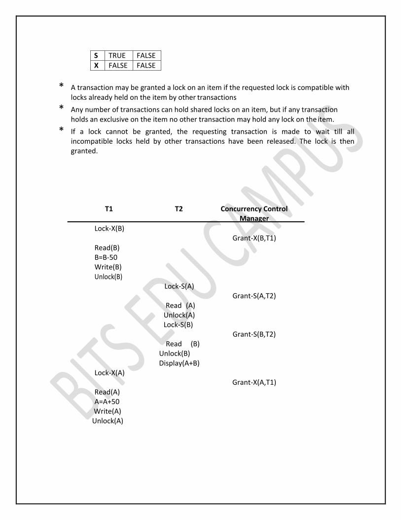
S TRUE FALSE
X FALSE FALSE
* A transaction may be granted a lock on an item if the requested lock is compatible with locks already held on the item by other transactions
* Any number of transactions can hold shared locks on an item, but if any transaction holds an exclusive on the item no other transaction may hold any lock on the item.
* If a lock cannot be granted, the requesting transaction is made to wait till all incompatible locks held by other transactions have been released. The lock is then granted.
T1 T2 Concurrency Control Manager
Lock-X(B)
Read(B) B=B-50 Write(B) Unlock(B)
Lock-X(A)
Read(A) A=A+50
Write(A) Unlock(A)
Lock-S(A)
Read (A) Unlock(A) Lock-S(B)
Read (B) Unlock(B) Display(A+B)
Grant-X(B,T1)
Grant-S(A,T2)
Grant-S(B,T2)
Grant-X(A,T1)
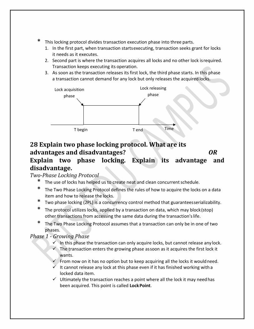
* This locking protocol divides transaction execution phase into three parts.1. In the first part, when transaction starts executing, transaction seeks grant for locks
it needs as it executes. 2. Second part is where the transaction acquires all locks and no other lock is required.
Transaction keeps executing its operation. 3. As soon as the transaction releases its first lock, the third phase starts. In this phase
a transaction cannot demand for any lock but only releases the acquired locks.
Lock acquisition
phase
Lock releasing
phase
T begin T end Time
28 Explain two phase locking protocol. What are its advantages and disadvantages? OR Explain two phase locking. Explain its advantage and disadvantage. Two-Phase Locking Protocol
* The use of locks has helped us to create neat and clean concurrent schedule.
* The Two Phase Locking Protocol defines the rules of how to acquire the locks on a data item and how to release the locks.
* Two phase locking (2PL) is a concurrency control method that guarantees serializability.
* The protocol utilizes locks, applied by a transaction on data, which may block (stop) other transactions from accessing the same data during the transaction's life.
* The Two Phase Locking Protocol assumes that a transaction can only be in one of two phases.
Phase 1 - Growing Phase In this phase the transaction can only acquire locks, but cannot release any lock. The transaction enters the growing phase as soon as it acquires the first lock it
wants. From now on it has no option but to keep acquiring all the locks it would need. It cannot release any lock at this phase even if it has finished working with a
locked data item. Ultimately the transaction reaches a point where all the lock it may need has
been acquired. This point is called Lock Point.
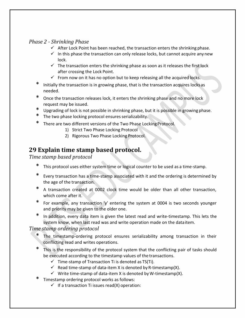
Phase 2 - Shrinking Phase After Lock Point has been reached, the transaction enters the shrinking phase. In this phase the transaction can only release locks, but cannot acquire any new
lock. The transaction enters the shrinking phase as soon as it releases the first lock
after crossing the Lock Point. From now on it has no option but to keep releasing all the acquired locks.
* Initially the transaction is in growing phase, that is the transaction acquires locks as needed.
* Once the transaction releases lock, it enters the shrinking phase and no more lock request may be issued.
* Upgrading of lock is not possible in shrinking phase, but it is possible in growing phase.
* The two phase locking protocol ensures serializability.
* There are two different versions of the Two Phase Locking Protocol.1) Strict Two Phase Locking Protocol
2) Rigorous Two Phase Locking Protocol.
29 Explain time stamp based protocol. Time stamp based protocol
* This protocol uses either system time or logical counter to be used as a time-stamp.
* Every transaction has a time-stamp associated with it and the ordering is determined by the age of the transaction.
* A transaction created at 0002 clock time would be older than all other transaction, which come after it.
* For example, any transaction 'y' entering the system at 0004 is two seconds younger and priority may be given to the older one.
* In addition, every data item is given the latest read and write-timestamp. This lets the system know, when last read was and write operation made on the data item.
Time stamp ordering protocol
* The timestamp-ordering protocol ensures serializability among transaction in their conflicting read and writes operations.
* This is the responsibility of the protocol system that the conflicting pair of tasks should be executed according to the timestamp values of the transactions. Time-stamp of Transaction Ti is denoted as TS(Ti). Read time-stamp of data-item X is denoted by R-timestamp(X). Write time-stamp of data-item X is denoted by W-timestamp(X).
* Timestamp ordering protocol works as follows: If a transaction Ti issues read(X) operation:
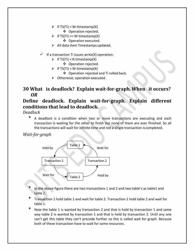
Held by Table 1
Wait for
If TS(Ti) < W-timestamp(X) Operation rejected.
If TS(Ti) >= W-timestamp(X) Operation executed.
All data-item Timestamps updated.
If a transaction Ti issues write(X) operation: If TS(Ti) < R-timestamp(X)
Operation rejected. If TS(Ti) < W-timestamp(X)
Operation rejected and Ti rolled back. Otherwise, operation executed.
30 What is deadlock? Explain wait-for-graph. When it occurs? OR Define deadlock. Explain wait-for-graph. Explain different conditions that lead to deadlock. Deadlock
* A deadlock is a condition when two or more transactions are executing and each transaction is waiting for the other to finish but none of them are ever finished. So all the transactions will wait for infinite time and not a single transaction is completed.
Wait-for-graph
* In the above figure there are two transactions 1 and 2 and two table’s as table1 and table 2.
* Transaction 1 hold table 1 and wait for table 2. Transaction 2 hold table 2 and wait for table 1.
* Now the table 1 is wanted by transaction 2 and that is hold by transaction 1 and same way table 2 is wanted by transaction 1 and that is hold by transaction 2. Until any one can’t get this table they can’t precede further so this is called wait for graph. Because both of these transaction have to wait for some resources.
Wait for Table 2 Hold by
Transaction 1 Transaction 2
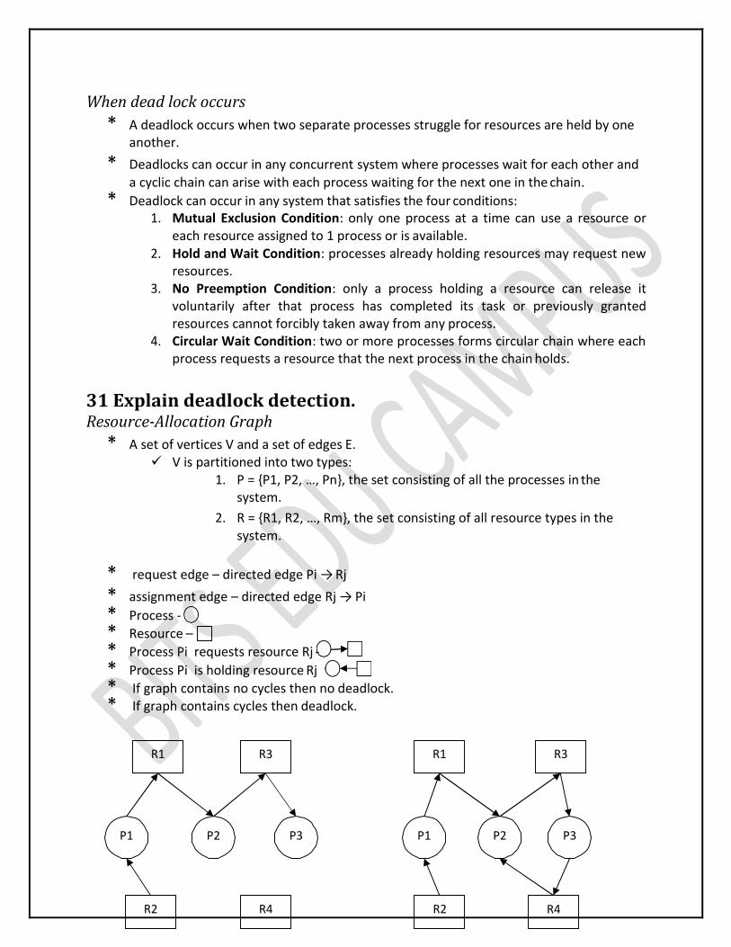
When dead lock occurs
* A deadlock occurs when two separate processes struggle for resources are held by one another.
* Deadlocks can occur in any concurrent system where processes wait for each other and a cyclic chain can arise with each process waiting for the next one in the chain.
* Deadlock can occur in any system that satisfies the four conditions:1. Mutual Exclusion Condition: only one process at a time can use a resource or
each resource assigned to 1 process or is available. 2. Hold and Wait Condition: processes already holding resources may request new
resources. 3. No Preemption Condition: only a process holding a resource can release it
voluntarily after that process has completed its task or previously granted resources cannot forcibly taken away from any process.
4. Circular Wait Condition: two or more processes forms circular chain where each process requests a resource that the next process in the chain holds.
31 Explain deadlock detection. Resource-Allocation Graph
* A set of vertices V and a set of edges E. V is partitioned into two types:
1. P = {P1, P2, …, Pn}, the set consisting of all the processes in the system.
2. R = {R1, R2, …, Rm}, the set consisting of all resource types in the system.
* request edge – directed edge Pi → Rj
* assignment edge – directed edge Rj → Pi
* Process -
* Resource –
* Process Pi requests resource Rj -
* Process Pi is holding resource Rj
* If graph contains no cycles then no deadlock.* If graph contains cycles then deadlock.
P1 P2 P3
R1 R3
R2 R4
P1 P2 P3
R1 R3
R2 R4
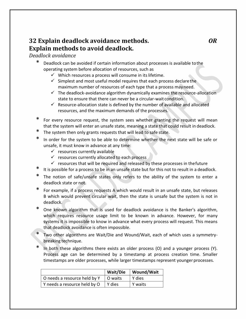
32 Explain deadlock avoidance methods. OR Explain methods to avoid deadlock. Deadlock avoidance
* Deadlock can be avoided if certain information about processes is available to the operating system before allocation of resources, such as Which resources a process will consume in its lifetime. Simplest and most useful model requires that each process declare the
maximum number of resources of each type that a process may need. The deadlock-avoidance algorithm dynamically examines the resource-allocation
state to ensure that there can never be a circular-wait condition. Resource-allocation state is defined by the number of available and allocated
resources, and the maximum demands of the processes.
* For every resource request, the system sees whether granting the request will mean that the system will enter an unsafe state, meaning a state that could result in deadlock.
* The system then only grants requests that will lead to safe state.
* In order for the system to be able to determine whether the next state will be safe or unsafe, it must know in advance at any time: resources currently available resources currently allocated to each process resources that will be required and released by these processes in the future
* It is possible for a process to be in an unsafe state but for this not to result in a deadlock.
* The notion of safe/unsafe states only refers to the ability of the system to enter a deadlock state or not.
* For example, if a process requests A which would result in an unsafe state, but releases B which would prevent circular wait, then the state is unsafe but the system is not in deadlock.
* One known algorithm that is used for deadlock avoidance is the Banker's algorithm, which requires resource usage limit to be known in advance. However, for many systems it is impossible to know in advance what every process will request. This means that deadlock avoidance is often impossible.
* Two other algorithms are Wait/Die and Wound/Wait, each of which uses a symmetry-
breaking technique.
* In both these algorithms there exists an older process (O) and a younger process (Y). Process age can be determined by a timestamp at process creation time. Smaller timestamps are older processes, while larger timestamps represent younger processes.
Wait/Die Wound/Wait
O needs a resource held by Y O waits Y dies
Y needs a resource held by O Y dies Y waits
33 Explain types of access control methods of data security OR Explain discretionary access control and mandatory access control of data security.
* There are two different methods of data access control:-1. Discretionary access control 2. Mandatory access control
Discretionary access control
* In this method, user is given access rights (privileges) to access database object or data items such as table or view.
* This method is based on the concept of access rights and mechanisms for giving rights to user.
* In this method a single user can have different rights on different data items, as well as different user can have different rights on the same data item.
* SQL support discretionary access control through the GRANT and REVOKE commands.
GRANT
* This command gives rights to user for a data items.Syntax:-
GRANT privilege ON object TO user [WITH GRANT OPTION]
REVOKE * This command takes back rights from user for a data items.
Syntax:- REVOKE privilege ON object FROM user {RESTRICT/CASCADE}
* Privileges are various operations that we will perform on table or view E.g. INSERT, UPDATE, DELETE, SELECT etc.
* Object is table or view or any data item.
* User is the name of user.
* With grant option is used if user wants to pass the rights to other user. Means if a user get a rights with the grant option then he/she can give this rights to another user.
* When user executes a REVOKE command with the cascade option then it will take back given rights from all the users who get those rights from this user.
Mandatory access control
* In this method individual user cannot get rights. But all the users as well as all the objects are classified into different categories. Each user is assigned a clearance level and each object is assigned a security level.
* A user can access object of particular security level only if he has proper clearance level.
* The DBMS determines whether a given user can read or write a given object based on some rules.
* This rule contains security level of object and clearance level of the user.
* This rule makes sure that sensitive data can never be passed to a user without necessary clearance.
Components
* The commonly used mandatory access control technique for multi-level security uses four components as given below
1. Subjects:-Such as users, accounts, programs etc. 2. Objects:-Such as relation (table), tuples (records), attribute (column), view etc. 3. Clearance level:-Such as top secret (TS), secret (S), confidential (C), Unclassified
(U). Each subject is classified into one of these four classes. 4. Security level: -Such as top secret (TS), secret (S), confidential (C), Unclassified
(U). Each object is classified into one of these four classes.
* In the above system TS>S>C>U, where TS>S means class TS data is more sensitive than class S data.
Rules:-
* A user can access data by following two rules1. Security property:-
Subject S will read object O if class (S)>=class (O) 2. Star (*) security property:-
Subject S will write object O if class (S) <=class (O)
34 Explain DDL, DML, DCL and DQL.
OR Describe component of SQL. DDL (Data Definition Language)
* It is a set of SQL commands used to create, modify and delete database objects such as
tables, views, indices, etc.
* It is normally used by DBA and database designers.
* It provides commands like: CREATE: to create objects in a database. ALTER: to alter the schema, or logical structure, of the database. DROP: to delete objects from the database. TRUNCATE: to remove all records from the table.
DML (Data Manipulation Language) * It is a set of SQL commands used to insert, modify and delete data in a database.
* It is normally used by general users who are accessing database via pre-developed applications.
* It provides commands like: INSERT: to insert data into a table.
UPDATE: to modify existing data in a table. DELETE: to delete records from a table. LOCK: to lock tables to provide concurrency control among multiple users.
DQL (Data Query Language) * It is a component of SQL that allows data retrieval from the database.
* It provides command like SELECT. This command is a heart of SQL, and allows data retrieval in different ways.
DCL (Data Control Language)
* It is set of SQL commands used to control access to data and database. Occasionally DCL commands are grouped with DML commands.
* It provides commands like: COMMIT: to save work permanently. ROLLBACK: to undo work and restore database to previous state. SAVEPOINT: to identify a point in a transaction to which work can be undone. GRANT: to give access privileges to users on the database. REVOKE: to withdraw access privileges given to users on the database.
1. REVOKE: The REVOKE is a command used to take back access or privileges or
rights on the database objects from the users.
Syntax:
REVOKE privilege_name
ON object_name
FROM {user_name |PUBLIC }
Explanation:
privilege_name is the access right or privilege want to take back from the user. Some of the access rights are ALL, EXECUTE, and SELECT.
object_name is the name of an database object like TABLE, VIEW, STORED PROC and SEQUENCE.
user_name is the name of the user from whom an access right is being taken back.
PUBLIC is used to take back access rights to all users.
35 Explain on delete cascade with example.
* A foreign key with cascade delete means that if a record in the Parent (Master) table is deleted, then the corresponding records in the Child (Foreign) table with automatically be deleted. This is called a cascade delete in Oracle.
* A foreign key with a cascade delete can be defined in either a CREATE TABLE statement or an ALTER TABLE statement.
* Syntax (Create table)CREATE TABLE table_name
( column1 datatype null/not null, column2 datatype null/not null,
...
CONSTRAINT fk_column FOREIGN KEY (column1, column2, ... column_n) REFERENCES parent_table (column1, column2, ... column_n)
ON DELETE CASCADE );
* Syntax (Alter table)ALTER TABLE table_name
ADD CONSTRAINT constraint_name
FOREIGN KEY (column1, column2, ... column_n)
REFERENCES parent_table (column1, column2, ... column_n)
ON DELETE CASCADE;
36 Write short note on stored procedure in PL/SQL. OR Explain stored procedures in PL/SQL.
* A stored procedure (proc) is a group of PL/SQL statements that performs specific task.
* A procedure has two parts, header and body.
* The header consists of the name of the procedure and the parameters passed to the procedure.
* The body consists of declaration section, execution section and exception section.
* A procedure may or may not return any value. A procedure may return more than one
value.
*
General Syntax to create a procedure CREATE [OR REPLACE] PROCEDURE proc_name [list of parameters] IS
BEGIN Declaration section
Execution section EXCEPTION
Exception section END;
Explanation
Create:-It will create a procedure. Replace:- It will re-create a procedure if it already exists. We can pass parameters to the procedures in three ways.
1. IN-parameters: - These types of parameters are used to send values to stored procedures.
2. OUT-parameters: - These types of parameters are used to get values from stored procedures. This is similar to a return type in functions but procedure can return values for more than one parameters.
3. IN OUT-parameters: - This type of parameter allows us to pass values into a procedure and get output values from the procedure.
IS indicates the beginning of the body of the procedure. The code between IS and BEGIN forms the Declaration section. Begin:-It contains the executable statement. Exception:- It contains exception handling part. This section is optional. End:- It will end the procedure. The syntax within the brackets [ ] indicates that they are optional. By using CREATE OR REPLACE together the procedure is created if it does not exist and if it exists then it is replaced with the current code.
Advantages of procedure
* Security:- We can improve security by giving rights to selected persons only.
* Faster Execution:- It is precompiled so compilation of procedure is not required every
time you call it.
* Sharing of code:- Once procedure is created and stored, it can be used by more than
one user.
* Productivity:- Code written in procedure is shared by all programmers. This eliminates
redundant coding by multiple programmers so overall improvement in productivity.
37 Explain database trigger with example. OR Write short note on database triggers in PL/SQL. OR What is trigger? Explain its type with their syntax.
* A trigger is a PL/SQL block structure which is triggered (executed) automatically when DML statements like Insert, Delete, and Update is executed on a table.
* There are two types of triggers based on the level it is triggered.1. Row level trigger - An event is triggered when any row of the table is changed
irrespective of insert, update or delete statement. 2. Statement level trigger - An event is triggered when particular SQL statement is
executed, e.g. trigger on insert command.
* We cannot pass parameters into triggers like stored procedure.* We cannot do transaction control (commit … rollback) in trigger.

* Triggers are normally slow.
* When triggers can be used,1. Based on change in one table, we want to update other table. 2. Automatically update derived columns whose values change based on other
columns. 3. Logging. 4. Enforce business rules.
Syntax of Trigger CREATE [OR REPLACE] TRIGGER trigger_name
[BEFORE / AFTER] [INSERT / UPDATE / DELETE [of columnname]]
ON table_name [REFERENCING [OLD AS old, NEW AS new]] [FOR EACH ROW [WHEN condition]]
DECLARE Declaration section
BEGIN Executable statements
END;
CREATE [OR REPLACE ] TRIGGER trigger_name:- This clause creates a trigger with the given name or overwrites an existing trigger. [BEFORE | AFTER]:- This clause indicates at what time the trigger should be fired. Before updating the table or after updating a table. [INSERT / UPDATE / DELETE]:- This clause determines on which kind of statement the trigger should be fired. Either on insert or update or delete or combination of any or all. More than one statement can be used together separated by OR keyword. The trigger gets fired at all the specified triggering event. [OF columnname]:- This clause is used when you want to trigger an event only when a specific column is updated. This clause is mostly used with update triggers. [ON table_name]:- This clause identifies the name of the table or view to which the trigger is related. [REFERENCING OLD AS old NEW AS new]:- This clause is used to reference the old and new values of the data being changed. By default, you reference the values as old. column_name or new.column_name. The reference names can also be changed from old or new to any other user-defined name. You cannot reference old values while inserting a record, or new values while deleting a record, because they do not exist. [FOR EACH ROW]:- This clause is used to determine whether a trigger must fire when each row gets affected ( i.e. a Row Level Trigger) or just once when the entire SQL statement is executed(i.e.statement level Trigger). WHEN (condition):- The trigger is fired only for rows that satisfy the condition specified. This clause is valid only for row level triggers.
38 What is cursor? Explain with example. OR Write short note on cursors and its types.
* Cursors are database objects used to traverse the results of a select SQL query.
* It is a temporary work area created in the system memory when a select SQL statement is executed.
* This temporary work area is used to store the data retrieved from the database, and manipulate this data.
* It points to a certain location within a record set and allow the operator to move forward (and sometimes backward, depending upon the cursor type).
* We can process only one record at a time.
* The set of rows the cursor holds which is called the active set (active data set).
* Cursors are often criticized for their high overhead.
* There are two types of cursors in PL/SQL:1. Implicit cursors:
These are created by default by ORACLE itself when DML statements like, insert, update, and delete statements are executed.
They are also created when a SELECT statement that returns just one row is executed.
We cannot use implicit cursors for user defined work. 2. Explicit cursors:
Explicit cursors are user defined cursors written by the developer. They can be created when a SELECT statement that returns more than
one row is executed. Even though the cursor stores multiple records, only one record can be
processed at a time, which is called as current row. When you fetch a row, the current row position moves to next row.
Attributes of Cursor:- Attributes Return Value Example %FOUND It will return TRUE, if the DML statements like INSERT,
DELETE, UPDATE and SELECT will affect at least one row else return FALSE
SQL%FOUND
%NOTFOUND It will return FALSE, if the DML statements like INSERT, DELETE, UPDATE and SELECT will affect at least one row else return TRUE
SQL%NOTFOUND
%ROWCOUNT Return the number of rows affected by the DML operations INSERT, DELETE, UPDATE, SELECT
SQL%ROWCOUNT
%ISOPEN It will return true if cursor is open else return false. SAL%OPEN
Steps to manage explicit cursor:- 1) Declare a cursor:-
A cursor is defined in the declaration section of PL/SQL block. Syntax:-
CURSOR cursorname IS SELECT ……… 2) Open a cursor:-
Once cursor is declared we can open it. When cursor is opened following operations are performed.
a. Memory is allocated to store the data. b. Execute SELECT statement associated with cursor c. Create active data set by retrieving data from table d. Set the cursor row pointer to point to first record in active data set.
Syntax:- OPEN cursorname;
3) Fetching data:- We cannot process selected row directly. We have to fetch column values of a row into memory variables. This is done by FETCH statement. Syntax:-
FETCH cursorname INTO variable1, variable2……….
4) Processing data:- This step involves actual processing of current row.
5) Closing cursor:- A cursor should be closed after the processing of data completes. Once you close the cursor it will release memory allocated for that cursor. Syntax:-
CLOSE cursorname;
Example:- DECLARE CURSOR emp_cur IS SELECT emp_rec FROM emp_tbl WHERE salary > 10000; BEGIN OPEN emp_cur; FETCH emp_cur INTO emp_rec; dbms_output.put_line (emp_rec.first_name || ' ' || emp_rec.last_name); CLOSE emp_cur; END;
Explanation:- In the above example, first we are delaring a cursor whose name is emp_cur with select
query.
In select query we have used where condition such that salary<10000. So active data set contain only such records whose salalry less than 10000.
Then, we are opening the cursor in the execution section.
Then we are fetching the records from cursor to the variable named emp_rec.

Then we are displaying the first_name and last_name of records fetched in variable.
At last as soon as our work completed we are closing the cursor.