data warehousing & data mining

6/2/2014

1

Data Warehousing & Data MiningWolf-Tilo BalkeKinda El MaarryInstitut für InformationssystemeTechnische Universität Braunschweighttp://www.ifis.cs.tu-bs.de

• Last Week: Optimization -Indexes for multidimensional data

– R-Trees

– UB-Trees

– Bitmap Indexes

• We continue this lecture with optimization…

Data Warehousing & OLAP – Wolf-Tilo Balke – Institut für Informationssysteme – TU Braunschweig 2

Summary

5. Optimization

5.1 Partitioning

5.2 Joins

5.3 Materialized Views

DW & DM – Wolf-Tilo Balke – Institut für Informationssysteme – TU Braunschweig 3

5. Optimization

• Breaking the data into several physical units that can be handled separately

• Granularity and partitioning arekey to efficient implementationof a warehouse

• The question is not whether to use partitioning, but how to do it


5.1 Partitioning

• Why partitioning?

– Flexibility in managing data

– Smaller physical units allow

• Inexpensive indexing

• Sequential scans, if needed

• Easy reorganization

• Easy recovery

• Easy monitoring


5.1 Partitioning

• In DWs, partitioning is done to improve:

– Business query performance, i.e., minimize the amount of data to scan

– Data availability, e.g., back-up/restores can run at the partition level

– Database administration, e.g., adding new columns to a table, archiving data, recreating indexes, loading tables


5.1 Partitioning

6/2/2014

2

• Possible approaches:– Data partitioning where data

is usually partitioned by• Date

• Line of business

• Geography

• Organizational unit

• Combinations of these factors

– Hardware partitioning• Makes data available to different processing nodes

• Sub-processes may run on specialized nodes


5.1 Partitioning

• Data partitioning levels

– Application level

– DBMS level

• Partitioning on DBMS level is obvious, but it also makes sense to partition at application level

– E.g., allows different definitions for each year

• Important, since DWs span many years and as business evolves DWs change, too

• Think for instance about changing tax laws


5.1 Data Partitioning

vs.

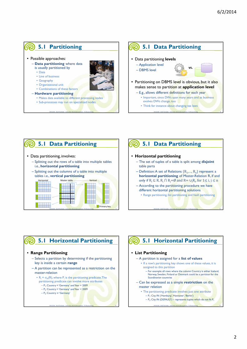
• Data partitioning, involves:

– Splitting out the rows of a table into multiple tables i.e., horizontal partitioning

– Splitting out the columns of a table into multiple tables i.e., vertical partitioning



Master tableHorizontal Vertical

Primary key

• Horizontal partitioning

– The set of tuples of a table is split among disjointtable parts

– Definition: A set of Relations {R1,…, Rn} represent a horizontal partitioning of Master-Relation R, if and only if Ri ⊆ R, Ri ⋂ Rj Ø and R ∪iRi, for 1≤ i, j ≤ n

– According to the partitioning procedure we have different horizontal partitioning solutions

• Range partitioning, list partitioning and hash partitioning



• Range Partitioning

– Selects a partition by determining if the partitioning key is inside a certain range

– A partition can be represented as a restriction on the master-relation

• Ri = σPi(R), where Pi is the partitioning predicate. The partitioning predicate can involve more attributes

– P1: Country = ‘Germany’ and Year = 2009

– P2: Country = ‘Germany’ and Year < 2009

– P3: Country ≠ ‘Germany’


5.1 Horizontal Partitioning

• List Partitioning

– A partition is assigned for a list of values

• If a row’s partitioning key shows one of these values, it is assigned to this partition

– For example: all rows where the column Country is either Iceland, Norway, Sweden, Finland or Denmark could be a partition for the Scandinavian countries

– Can be expressed as a simple restriction on the master relation

• The partitioning predicate involves just one attribute

– P1: City IN (‘Hamburg’, ‘Hannover’, ‘Berlin’)

– P2: City IN (DEFAULT) – represents tuples which do not fit P1



6/2/2014

3

• Hash Partitioning

– The value of a hash function determines membership in a partition

• This kind of partitioning is often used in parallel processing

• The choosing of the hash function is decisive: the goal is to achieve an equal distribution of the data

– For each tuple t, of the master-table R, the hash function will associate it to a partition table Ri

• Ri {t1, …, tm/tj∈R and H(tj) = H(tk) for 1 ≤ j, k ≤ m}



• In DW, data is partitioned by the– Time dimension

• Periods, such as week or month can be used or the data can be partitioned by the age of the data

• E.g., if the analysis is usually done on last month's data the table could be partitioned into monthly segments

– Some dimension other than time• If queries usually run on a grouping of data: e.g. each branch tends

to query on its own data and the dimension structure is not likely to change then partition the table on this dimension

– Table size• If a dimension cannot be used, partition the table by a

predefined size. If this method is used, metadata must be created to identify what is contained in each partition



• Vertical Partitioning

– Involves creating tables with fewer columns and using additional tables to store the remaining columns

• Usually called row splitting

• Row splitting creates one-to-one relationships between the partitions

– Different physical storage might be used e.g., storing infrequently used or very wide columns on a different device


5.1 Vertical Partitioning

• In DW, common vertical partitioning means

– Moving seldom used columns from a highly-used table to another table

– Creating a view across the two newly created tables restores the original table with a performance penalty

• However, performance will increase when accessing the highly-used data e.g. for statistical analysis



• In DWs with very large dimension tables like the customer table of Amazon (tens of millions of records)

– Most of the attributes are rarely –if at all– queried

• E.g. the address attribute is not as interesting for marketing as evaluating customers per age-group

– But one must still maintain the link between the fact table and the complete customer dimension, which has high performance costs!



• The solution is to use Mini-Dimensions, a special case of vertical partitioning

– Many dimension attributes are used very frequently as browsing constraints

• In big dimensions these constraints can be hard to find among the lesser used ones

– Logical groups of often used constraints can be separated into small dimensions which are very well indexed and easily accessible for browsing



6/2/2014

4

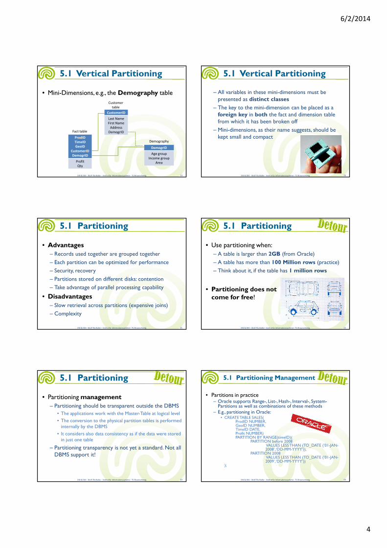
• Mini-Dimensions, e.g., the Demography table



ProdID

TimeID

GeoID

CustomerID

DemogrID

Profit

Qty

CustomerID

Last Name

First Name

Address

DemogrID

DemogrID

Age group

Income group

Area

Fact table

Customer

table

Demography

– All variables in these mini-dimensions must be presented as distinct classes

– The key to the mini-dimension can be placed as a foreign key in both the fact and dimension tablefrom which it has been broken off

– Mini-dimensions, as their name suggests, should be kept small and compact



• Advantages

– Records used together are grouped together

– Each partition can be optimized for performance

– Security, recovery

– Partitions stored on different disks: contention

– Take advantage of parallel processing capability

• Disadvantages

– Slow retrieval across partitions (expensive joins)

– Complexity


5.1 Partitioning

• Use partitioning when:

– A table is larger than 2GB (from Oracle)

– A table has more than 100 Million rows (practice)

– Think about it, if the table has 1 million rows

• Partitioning does not come for free!


5.1 Partitioning

• Partitioning management

– Partitioning should be transparent outside the DBMS

• The applications work with the Master-Table at logical level

• The conversion to the physical partition tables is performed internally by the DBMS

• It considers also data consistency as if the data were stored in just one table

– Partitioning transparency is not yet a standard. Not all DBMS support it!


5.1 Partitioning

• Partitions in practice– Oracle supports Range-, List-, Hash-, Interval-, System-

Partitions as well as combinations of these methods– E.g., partitioning in Oracle:

• CREATE TABLE SALES(ProdID NUMBER,GeoID NUMBER,TimeID DATE,Profit NUMBER)PARTITION BY RANGE(timeID)(

PARTITION before 2008VALUES LESS THAN (TO_DATE (’01-JAN-2008’, ‘DD-MM-YYYY’)),

PARTITION 2008VALUES LESS THAN (TO_DATE (’01-JAN-2009’, ‘DD-MM-YYYY’))

);


5.1 Partitioning Management

6/2/2014

5

• In Oracle partitioning is performed with the help of only one function - LESS THAN

– Partition data in the current year

• ALTER TABLE SalesADD PARTITION after 2009 VALUES LESS THAN

(MAXVALUE);



• Partitioning:



RowID ProdID GeoID TimeID Profit

… … … … …

121 132 2 05.2007 8K

122 12 2 08.2008 7K

123 15 1 09.2007 5K

124 14 3 01.2009 3K

125 143 2 03.2009 1,5K

126 99 3 05.2007 1K

… … … …


… … … … …

121 132 2 05.2007 8K

123 15 1 09.2007 5K

126 99 3 05.2007 1K


122 12 2 08.2008 7K


124 14 3 01.2009 3K

125 143 2 03.2009 1,5K

• In the data cleaning phase, records can be updated. For partition split tables, this means data migration:

– UPDATE Sales SET TimeID= ‘05.2008' WHERE RowID= 121;

• ERROR at line 1: ORA-14402: updating partition key columnwould cause a partition change




… … … … …

121 132 2 05.2007 8K

123 15 1 09.2007 5K

126 99 3 05.2007 1K


122 12 2 08.2008 7K


124 14 3 01.2009 3K

125 143 2 03.2009 1,5K

• Data migration between partitions is by default disabled

– ALTER TABLE Sales ENABLE ROW MOVEMENT;

– ROW MOVEMENT deletes the record from one partition and inserts it into another

• The issue is that RowID is automatically changed!




… … … … …

121 132 2 05.2007 8K

123 15 1 09.2007 5K

126 99 3 05.2007 1K


122 12 2 08.2008 7K

13256 132 2 05.2008 8k

• Often queries over several partitions are needed

– This results in joins over the data

– Though joins are generally expensive operations, the overall cost of the query may strongly differ with the chosen evaluation plan for the joins

• Joins are commutative and associative

– R⋈S≡S⋈R

– R⋈(S ⋈T) ≡(S⋈R) ⋈T


5.2 Join Optimization

• This allows to evaluate individual joinsin any order

– Results in join trees

• Different join trees may show very differentevaluation performance

– Join trees have different shapes

– Within a shape, there are different relation assignments possible

• Example: R⋈S⋈T⋈U



⋈⋈

⋈⋈

⋈⋈

R S

T

U

⋈⋈

⋈⋈

⋈⋈

R S T U

6/2/2014

6

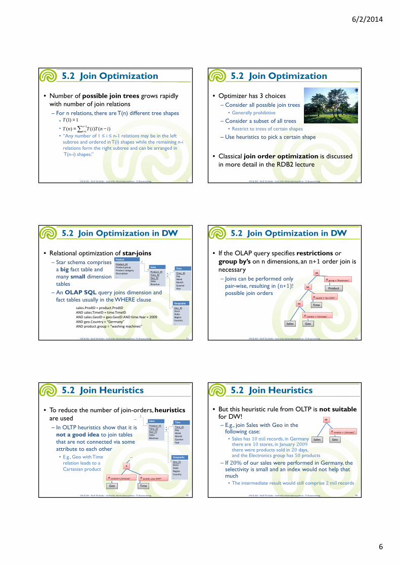
• Number of possible join trees grows rapidly with number of join relations

– For n relations, there are T(n) different tree shapes

••• “Any number of 1 ≤ i ≤ n-1 relations may be in the left

subtree and ordered in T(i) shapes while the remaining n-irelations form the right subtree and can be arranged inT(n-i) shapes.”



∑−

=−=

=1

1)()()(

1)1(n

iinTiTnT

T

• Optimizer has 3 choices

– Consider all possible join trees

• Generally prohibitive

– Consider a subset of all trees

• Restrict to trees of certain shapes

– Use heuristics to pick a certain shape

• Classical join order optimization is discussed in more detail in the RDB2 lecture



• Relational optimization of star-joins

– Star schema comprisesa big fact table andmany small dimensiontables

– An OLAP SQL query joins dimension and fact tables usually in the WHERE clause


5.2 Join Optimization in DW

Sales

Product_ID

Time_ID

Geo_ID

Sales

Revenue

Product

Product_ID

Product group

Product category

Description

…

Geography

Geo_ID

Store

State

Region

Country

…

Time

Time_ID

Day

Week

Month

Quarter

Year

n

n

n

1

1

1

sales.ProdID = product.ProdID

AND sales.TimeID = time.TimeID

AND sales.GeoID = geo.GeoID AND time.Year = 2009

AND geo.Country = “Germany”

AND product.group = “washing machines”

• If the OLAP query specifies restrictions or group by’s on n dimensions, an n+1 order join is necessary

– Joins can be performed onlypair-wise, resulting in (n+1)!

possible join orders


5.2 Join Optimization in DW

⋈⋈

⋈⋈

⋈⋈

Sales Geo

Time

Product

σ country = ‘Germany‘σ country = ‘Germany‘

σ month = ‘Jan 2009‘σ month = ‘Jan 2009‘

σ group = ‘Electronics‘σ group = ‘Electronics‘

• To reduce the number of join-orders, heuristicsare used

– In OLTP heuristics show that it isnot a good idea to join tablesthat are not connected via some attribute to each other

• E.g., Geo with Timerelation leads to aCartesian product


5.2 Join Heuristics

Sales

Product_ID

Time_ID

Geo_ID

Sales

Revenue

Geography

Geo_ID

Store

State

Region

Country

…

Time

Time_ID

Day

Week

Month

Quarter

Year

n

n

n

1

1

1

55

Geo Time

σ country=„Germany“σ country=„Germany“ σ month=„Jan 2009“σ month=„Jan 2009“

…

…

• But this heuristic rule from OLTP is not suitable for DW!– E.g., join Sales with Geo in the

following case: • Sales has 10 mil records, in Germany

there are 10 stores, in January 2009there were products sold in 20 days, and the Electronics group has 50 products

– If 20% of our sales were performed in Germany, the selectivity is small and an index would not help that much

• The intermediate result would still comprise 2 mil records


5.2 Join Heuristics

⋈⋈

Sales Geo

σ country = „Germany“σ country = „Germany“

6/2/2014

7

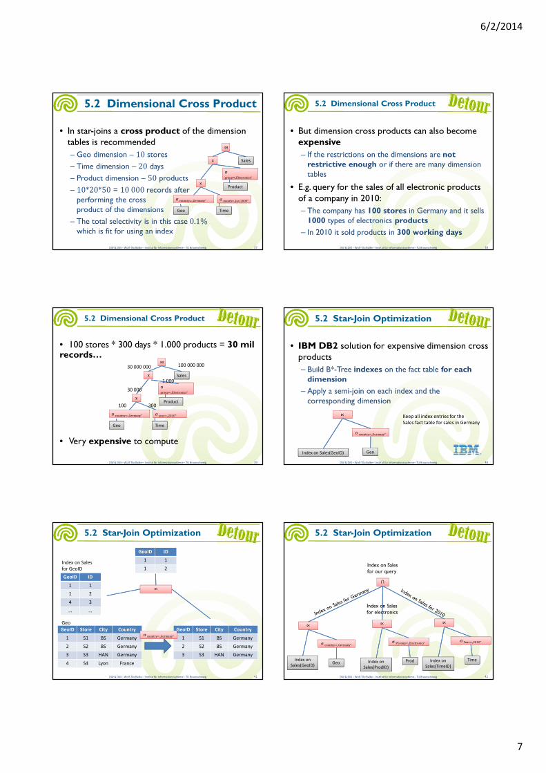
• In star-joins a cross product of the dimension tables is recommended

– Geo dimension – 10 stores

– Time dimension – 20 days

– Product dimension – 50 products

– 10*20*50 = 10 000 records afterperforming the crossproduct of the dimensions

– The total selectivity is in this case 0.1%

which is fit for using an index


5.2 Dimensional Cross Product

55

55

⋈⋈

Geo Time

Product

σ country=„Germany“σ country=„Germany“ σ month=„Jan 2009“σ month=„Jan 2009“

σgroup=„Electronics“


Sales

• But dimension cross products can also become expensive

– If the restrictions on the dimensions are not restrictive enough or if there are many dimension tables

• E.g. query for the sales of all electronic products of a company in 2010:

– The company has 100 stores in Germany and it sells 1000 types of electronics products

– In 2010 it sold products in 300 working days



• 100 stores * 300 days * 1.000 products = 30 mil records…

• Very expensive to compute



55

55

⋈⋈

Geo Time

Product

σ country=„Germany“σ country=„Germany“ σ year=„2010“σ year=„2010“



Sales

30 000

100 300

30 000 000

1 000

100 000 000

• IBM DB2 solution for expensive dimension cross products

– Build B*-Tree indexes on the fact table for each dimension

– Apply a semi-join on each index and the corresponding dimension


5.2 Star-Join Optimization

Geo

σ country=„Germany“σ country=„Germany“

⋉⋉

Index on Sales(GeoID)

Keep all index entries for the

Sales fact table for sales in Germany



GeoID Store City Country

1 S1 BS Germany

2 S2 BS Germany

3 S3 HAN Germany

4 S4 Lyon France

GeoID ID

1 1

1 2

4 3

… …

GeoID ID

1 1

1 2

⋉⋉

Geo

Index on Sales

for GeoID

GeoID Store City Country

1 S1 BS Germany

2 S2 BS Germany

3 S3 HAN Germany




Geo


⋉⋉

Index on

Sales(GeoID)Prod

σ PGroup=„Electronics“σ PGroup=„Electronics“

⋉⋉

Index on

Sales(ProdID)

Time

σ Year=„2010“σ Year=„2010“

⋉⋉

Index on

Sales(TimeID)

⋂⋂

Index on Sales for electronics

Index on Sales for our query

6/2/2014

8

• Materialized Views (MV)

– Views whose tuples are storedin the database are said to bematerialized

– They provides fast access, like a (very high-level) cache

– Need to maintain the view as the underlying tables change

• Ideally, we want incremental view maintenance algorithms



• How can we use MV in DW?– E.g., we have queries requiring us to join the Sales table

with another table and aggregate the result• SELECT P.Categ, SUM(S.Qty) FROM Product P, Sales S WHERE

P.ProdID=S.ProdID GROUP BY P.Categ

• SELECT G.Store, SUM(S.Qty) FROM Geo G, Sales S WHERE G.GeoID=S.GeoID GROUP BY G.Store

• ….

– There are more solutions to speed up such queries• Pre-compute the two joins involved (product with sales and geo

with sales)

• Pre-compute each query in its entirety

• Or use an already materialized view



• Having the following view materialized

– CREATE MATERIALIZED VIEW Totalsales (ProdID, GeoID, total) AS SELECT S.ProdID, S.GeoID, SUM(S.Qty) FROM Sales S GROUP BY S.ProdID, S.GeoID

• We can use it in our 2 queries

– SELECT P.Categ, SUM(T.Total) FROM Product P, TotalsalesT WHERE P.ProdID=T.ProdID GROUP BY P.Categ

– SELECT G.Store, SUM(T.Total) FROM Geo G, Totalsales T WHERE G.GeoID=T.GeoID GROUP BY G.Store



• MV issues

– Utilization

• What views should we materialize, and what indexes should we build on the pre-computed results?

– Choice of materialized views

• Given a query and a set of materialized views, can we use the materialized views to answer the query?

– Maintenance

• How frequently should we refresh materialized views to make them consistent with the underlying tables?

• And how can we do this incrementally?



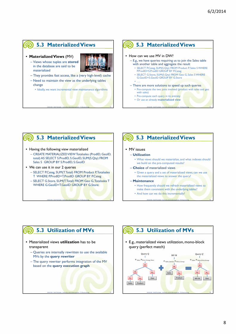
• Materialized views utilization has to be transparent

– Queries are internally rewritten to use the available MVs by the query rewriter

– The query rewriter performs integration of the MV based on the query execution graph


5.3 Utilization of MVs

• E.g., materialized views utilization, mono-block query (perfect match)


5.3 Utilization of MVs

⋈⋈

σFσF

Sales Product

⋈⋈

GeoσPσP

σGσG

σ Sales πPrice, Group, Store

Query Q

⋈⋈

Sales

Product

σPσP

σ Sales, Invoice π Price, Group

MV M

σFσF

MV M

⋈⋈

Geo

σGσG

σ Sales π Store,Price,Group

Query Q`

6/2/2014

9

• Integration of MV

– Valid replacement: A query Q` represents a valid replacement of query Q by utilizing the materialized view M, if Q and Q` always deliver the same result set

– For general relational queries, the problem of finding a valid replacement is NP-complete

• But there are practically relevant solutions for special cases like star-queries


5.3 Integration of MVs

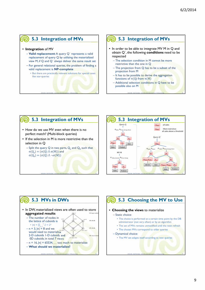
• In order to be able to integrate MV M in Q and obtain Q`, the following conditions need to be respected– The selection condition in M cannot be more

restrictive than the one in Q

– The projection from Q has to be a subset of the projection from M

– It has to be possible to derive the aggregation functions of π(Q) from π(M)

– Additional selection conditions in Q have to be possible also on M



• How do we use MV even when there is no perfect match? (Multi-block queries)

• If the selection in M is more restrictive than the selection in Q

– Split the query Q in two parts, Qa and Qb such that σ(Qa) = (σ(Q) ⋀ σ(M)) andσ(Qb) = (σ(Q) ⋀ ¬σ(M))





⋈⋈

σF[Q]σF[Q]

Sales Product

⋈⋈

GeoσPσP

σGσG

σSales πPrice, Group, Store

Query Q

⋈⋈

Sales Product

σPσP

σ Sales, Invoice πPrice, Group

MV M

σF[M]σF[M]

σF[Q] ⋀ σF[M]σF[Q] ⋀ σF[M]

MV M

⋈⋈

Geo

σGσG

σSales πStore

Query Q`

⋈⋈

⋈⋈

Sales

σF[Q] ⋀ ¬σF[M]σF[Q] ⋀ ¬σF[M]

Product

σPσP

σ Sales πPrice, Group, Store

∪ALL∪ALL

σF[Q]σF[Q] - all sales

σF[M]σF[M] - More restrictive:

all sales above a threshold

• In DW, materialized views are often used to store aggregated results– The number of nodes in

the lattice of cuboids is• |n| = ∏

j=1

n2 = 2n

– n = 3, |n| = 8 and we would need to materialize 2-D cuboids 1-D cuboids and0D cuboids; in total 7 views

– n = 16, |n| = 65534, … too much to materialize

– What should we materialize?


5.3 MVs in DWs

• Choosing the views to materialize

– Static choice:

• The choice is performed at a certain time point by the DB administrator (not very often) or by an algorithm

• The set of MVs remains unmodified until the next refresh

• The chosen MVs correspond to older queries

– Dynamical choice:

• The MV set adapts itself according to new queries


5.3 Choosing the MV to Use

6/2/2014

10

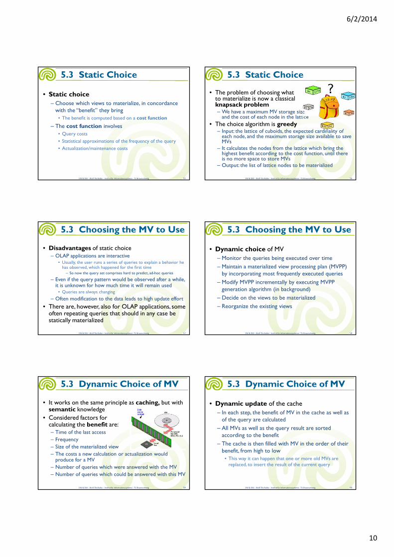
• Static choice

– Choose which views to materialize, in concordance with the “benefit” they bring

• The benefit is computed based on a cost function

– The cost function involves

• Query costs

• Statistical approximations of the frequency of the query

• Actualization/maintenance costs


5.3 Static Choice

• The problem of choosing what to materialize is now a classicalknapsack problem– We have a maximum MV storage size

and the cost of each node in the lattice

• The choice algorithm is greedy– Input: the lattice of cuboids, the expected cardinality of

each node, and the maximum storage size available to save MVs

– It calculates the nodes from the lattice which bring the highest benefit according to the cost function, until there is no more space to store MVs

– Output: the list of lattice nodes to be materialized


5.3 Static Choice

• Disadvantages of static choice– OLAP applications are interactive

• Usually, the user runs a series of queries to explain a behavior he has observed, which happened for the first time

– So now the query set comprises hard to predict, ad-hoc queries

– Even if the query pattern would be observed after a while, it is unknown for how much time it will remain used

• Queries are always changing

– Often modification to the data leads to high update effort

• There are, however, also for OLAP applications, some often repeating queries that should in any case be statically materialized



• Dynamic choice of MV

– Monitor the queries being executed over time

– Maintain a materialized view processing plan (MVPP) by incorporating most frequently executed queries

– Modify MVPP incrementally by executing MVPP generation algorithm (in background)

– Decide on the views to be materialized

– Reorganize the existing views



• It works on the same principle as caching, but with semantic knowledge

• Considered factors forcalculating the benefit are:– Time of the last access

– Frequency

– Size of the materialized view

– The costs a new calculation or actualization would produce for a MV

– Number of queries which were answered with the MV

– Number of queries which could be answered with this MV


5.3 Dynamic Choice of MV

• Dynamic update of the cache

– In each step, the benefit of MV in the cache as well as of the query are calculated

– All MVs as well as the query result are sorted according to the benefit

– The cache is then filled with MV in the order of their benefit, from high to low

• This way it can happen that one or more old MVs are replaced, to insert the result of the current query


5.3 Dynamic Choice of MV

6/2/2014

11

• Maintenance of MV

– Keeping a materialized view up-to-date with the underlying data

– Important questions

• How do we refresh a view when an underlying table is refreshed?

• When should we refresh a view in response to a change in the underlying table?


5.3 Maintenance of MV

• Materialized views can be maintained by re-computation on every update

– Not the best solution

• A better option is incremental view maintenance


5.3 How to Refresh a MV

• Incremental view maintenance

– Changes to database relations are used to compute changes to the materialized view, which is then updated

– Considering that we have a materialized view V, and that the basis relations suffer modifications through inserts, updates or deletes, we can calculate V` as follows

• V` = (V - ∆-)∪∆+,where ∆- and∆+represent deleted respectively inserted tuples


5.3 How to Refresh a MV

• Immediate

– As part of the transaction that modifies the underlying data tables

• Advantage: materialized view is always consistent

• Disadvantage: updates are slowed down

• Deferred

– Some time later, in a separate transaction

• Advantage: can scale to maintain many views without slowing updates

• Disadvantage: view briefly becomes inconsistent


5.3 When to Refresh a MV

• Deferred refresh comes in 3 flavors

– Lazy: delay refresh until next query on view, then refresh before answering the query

– Periodic (Snapshot): refresh periodically; queries are possibly answered using outdated version of view tuples; widely used for DW

– Event-based: e.g., refresh after a fixed number of updates to underlying data tables


5.3 When to Refresh a MV

• Partitioning: Horizontal or Vertical

– Records used together are grouped together

– However: slow retrieval across partitions

– Mini-Dimensions

• Joins: for DW it is sometimes better to perform cross product on dimensions first

• Materialized Views: we can’t materialize everthing

– Static or Dynamic choice of what to materialize

– The benefit cost function is decisive

Data Warehousing & OLAP – Wolf-Tilo Balke – Institut für Informationssysteme – TU Braunschweig 66

Summary

6/2/2014

12

• Queries!

– OLAP queries

– SQL for DW

– MDX


Next lecture

data warehousing & data mining

Documents