data warehousing - synthesis.ipi.ac.rusynthesis.ipi.ac.ru/synthesis/student/bigdata/lectures/dw 8...
TRANSCRIPT

Data Warehousing ETL

References
2
Christian S. Jensen, Torben Bach Pedersen, Christian Thomsen.
Introduction to Data Warehousing and Business Intelligence.
Course Data Warehousing and Machine Learning, Aalborg
University, Denmark
Wolf-Tilo Balke, Silviu Homoceanu. Data Warehousing & Data
Mining. Institut für Informationssysteme, Technische Universität
Braunschweig
Elena Baralis. Data warehouse: Architectures and processes.
Politecnico di Torino
J. Gamper. Extract-Transform-Load. Free University of Bolzano
IBM InfoSphere DataStage Essentials. Course KM201
IBM InfoSphere Warehouse 10 & Smart Analytics System
Bootcamp

Outline
3
The ETL Process
Phases, architecture
Data staging area, data structures
ETL construction: plan, building dimensions, building fact tables
Extract
Transformations
Data cleansing
Data integration
Load
IBM InfoSphere DataStage
Aim, architecture, job developing
Parallelism, partitioning
Combining data

4

ETL
5
When should we ETL ?
Periodically (e.g., every night, every week) or after significant events
Refresh policy set by administrator based on user needs and traffic
Possibly different policies for different sources
ETL is used to integrate heterogeneous systems
With different DBMS, operating system, hardware, communication protocols
ETL challenges
Getting the data from the source to target as fast as possible
Allow recovery from failure without restarting the whole process

6

ETL/DW Refreshment
7

ETL in the DW Architecture
8

Data Staging Area (DSA)
9
Transit storage for data in the ETL process, owned by the ETL team No indexes, no aggregations, no presentation access, no user querying, no service
level agreements
Transformations/cleansing done here
Users are not allowed in the staging area for any reason
Reports cannot access data in the staging area tables can be added, or dropped without modifying the user community
Only ETL processes can read/write the staging area ETL developers must capture table names, update strategies, load frequency, ETL
jobs, expected growth and other details about the staging area
Sequential operations on large data volumes Performed by central ETL logic
Easily restarted
No need for locking, logging, etc.
Consists of both RDBMS tables and data files
Finished dimensions copied from DSA to relevant marts
Allows centralized backup/recovery Backup/recovery facilities needed
Better to do this centrally in DSA than in all data marts

DSA Structures for Holding Data
10
Flat files
XML data sets
Relational tables

Flat Files
11
ETL tools based on scripts (Perl, VBScript, JavaScript, IBM – Orchestrate SHell Script)
Advantages
No overhead of maintaining metadata as DBMS does
Sorting, merging, deleting, replacing and other data-migration functions are much faster outside the DBMS
Disadvantages
No concept of updating
Queries and random access lookups are not well supported by the operating system
Flat files can not be indexed for fast lookups
When should flat files be used?
Staging source data for safekeeping and recovery
Best approach to restart a failed process is by having data dumped in a flat file
Sorting data
Sorting data in a file system may be more efficient as performing it in a DBMS with order_by clause
Sorting is important: a huge portion of the ETL processing cycles goes to sorting
Filtering
Using grep-like functionality
Replacing text strings
Sequential file processing is much faster at the system-level than it is with a database

XML Data sets
12
Used as common format for both input and output from the ETL
system
Generally, not used for persistent staging
Useful mechanisms
XML schema
XQuery, XPath
XSLT

Relational Tables
13
Using tables is most appropriate especially when there are no
dedicated ETL tools
Advantages
Apparent metadata: column names data types and lengths, cardinality, etc.
Relational abilities: data integrity as well as normalized staging
Open repository/SQL interface: easy to access by any SQL compliant tool
Disadvantages
Sometimes slower than the operating file system

Staging Area - Storage
14
How is the staging area designed?
Staging database, file system, and directory structures are set up by the DB and
OS administrators based on ETL architect estimations e.g., tables volumetric
worksheet

15

16

The Basic Structure of a Dimension
17

Primary Keys and Natural Keys: Example
18
Slowly Changing Dimensions (SCDs): change slowly but
unpredictably, rather than according to a regular schedule
SCD management methodology Type 2: add new row
historical data are tracked by creating multiple records for a given natural key
in the dimensional tables with separate surrogate keys and/or different version
numbers
unlimited history is preserved for each insert

Generating Surrogate Keys for Dimensions
19

Building Dimensions
20
Static dimension table
DW key assignment: production keys to DW keys using table
Combination of data sources: find common key ?
Check one-one and one-many relationships (using sorting)
Handling dimension changes
Find the newest DW key for a given production key
Table for mapping production keys to DW keys must be maintained and
updated
Load of dimensions
Small dimensions: replace
Large dimensions: load only changes

Building Big Dimensions from Multiple Sources
21

How to Check 1-to-1 and 1-to-many
22

The Grain of a Dimension
23

The Basic Load Plan for a Dimension
24

25

Extract
26

Extraction: Export and Extract
27
Data needs to be taken from a data source so that it can be put into
the DW
Internal scripts/tools at the data source, which export the data to be used
External programs, which extract the data from the source
If the data is exported, it is typically exported into a text file that
can then be brought into an intermediary database
If the data is extracted from the source, it is typically transferred
directly into an intermediary database

Extraction Methods
28

Extraction: Types of Data to be Extracted
29

Types of Extracts
30

31
32

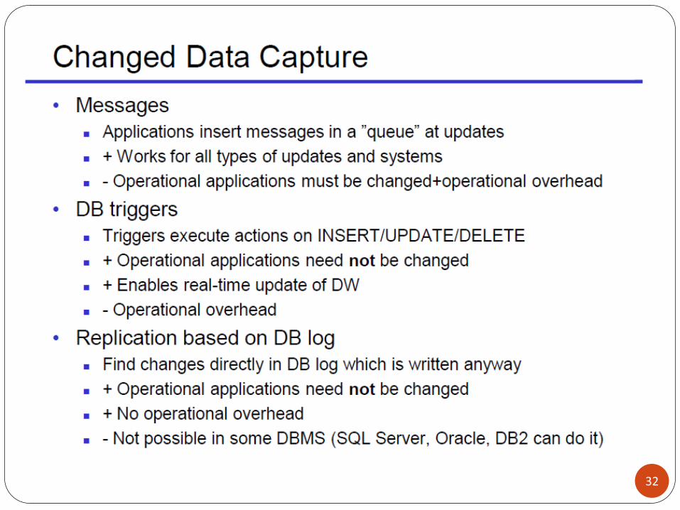
Incremental Extraction
33

Incremental Extraction
34
Application assisted
data modifications are captured by ad hoc application functions
requires changing OLTP applications (or APIs for database access)
increases application load
hardly avoidable in legacy systems
Log based
log data is accessed by means of appropriate APIs
log data format is usually proprietary
efficient, no interference with application load
Trigger based
triggers capture interesting data modifications
does not require changing OLTP applications
increases application load
Timestamp based
modified records are marked by the (last) modification timestamp
requires modifying the OLTP database schema (and applications)
deferred extraction, may lose intermediate states if data is transient
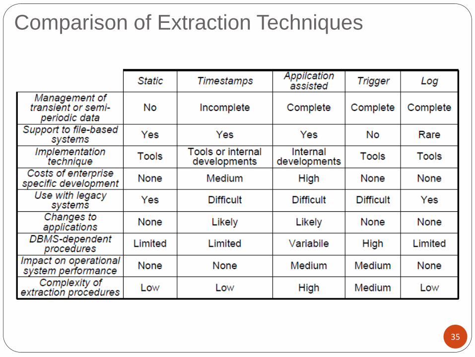
Comparison of Extraction Techniques
35

Transform
36

Transformation
37
Main step where the ETL adds value
Actually changes data and provides guidance whether data can be
used for its intended purposes
Performed in staging area
2 major steps
Data Cleaning
May involve manual work
Assisted by artificial intelligence algorithms and pattern recognition
Data Integration
May also involve manual work

38

Transform: Data Cleansing
39

40

41

The High Cost of Low Quality Data
42

Data Quality Importance
43

Data Quality Semi-automatic Tools
44
Commercial software
SAP Business Objects
IBM InfoSphere Data Stage
Oracle Data Quality and Oracle Data Profiling
Open source tools
Eobjects DataCleaner
Talend Open Profiler
…

Deliverables of Data Cleaning
Data-profiling results
Meta-data repository describing schema definitions, business objects, domains,
data sources, table definitions, data rules, value rules, etc.
Represents a quantitative assessment of original data sources
Error event table
Structured as a dimensional star schema
Each data quality error identified by the cleaning subsystem is inserted as a
row in the error event fact table
Audit dimension
Describes the data-quality context of a fact table
record being loaded into the DW
Attached to each fact record
Aggregates the information from the error event table
on a per record basis
45

Error Event Schema
46

Data Quality Process Flow Fatal errors events
daily sales from
several stores are
completely missing
an impossible invalid
value for an important
column has appeared
for which there are no
transformation rules
47

Screening
48
Each screen acts as a constraint or data rule and filters the incoming
data by testing one specific aspect of quality
Screen categories
Column screens – rules based on one single column
Mandatory columns containing null values
Values not adhering to a predefined list of values
Numeric values not fitting within a predefined range
Structure screens – rules based on multiple columns
Invalid hierarchical roll ups
Invalid parent - child relationships
Invalid foreign key – parent key relationships
Invalid code – description relationships
Business rule screens – complex rules
“Key account” customers should have at least 100.000 euro revenue in a predefined
period

Anomaly Detection
Count the rows in a table while grouping on
the column in question
SELECT state, count(*)
FROM order_detail GROUP BY state
What if our table has 100 million rows with
250,000 distinct values?
Use data sampling
Divide the whole data into 1000 pieces,
and choose 1 record from each
Add a random number column to the data,
sort it an take the first 1000 records
Common mistake is to select a range of dates
Most anomalies happen temporarily
49

Data Profiling
50
Pay closer look at strange values (outlier detection)
Observe data distribution patterns
Gaussian distribution
SELECT AVERAGE(sales_value) – 3 * STDDEV(sales_value),
AVERAGE(sales_value) + 3 * STDDEV(sales_value)
INTO Min_resonable, Max_resonable
Flat distribution
Identifier distributions (keys)
Zipfian distribution
Some values appear more often than others
In sales, more cheap goods are sold than
expensive ones
Pareto, Poisson, S distribution
Distribution discovery
Statistical software: SPSS, StatSoft, R, etc.

51

Comparing Strings
52
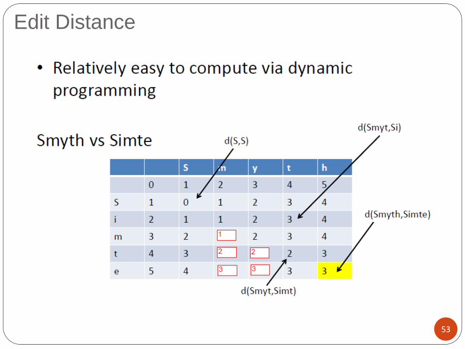
Edit Distance
53

Approximate Join
54
The join operation should be executed based on common fields, not
representing the customer identifier

Purge/Merge problem
55
Duplicate tuples should be identified and removed
A criterion is needed to evaluate record similarity

Data Mining Transformations
56

Data Cleaning Resume for DW Design
57

Transformation
58

Data Cleaning and Transformation Example
59

Transform: Data Integration
60

Data Integration
61

Schema Integration
62

Preintegration Analysis
63
A close look on the individual conceptual schemas to decide for an
adequate integration strategy
The larger the number of constructs, the more important is modularization
Is it really sensible/possible to integrate all schemas?

Schema conflicts
64

Schema Integration
65

Schema Integration
66
Schema integration is a semantic process
This usually means a lot of manual work
Computers can support the process by matching some (parts of) schemas
There have been some approaches towards (semi-)automatic
matching of schemas
Matching is a complex process and usually only focuses on simple constructs
like ‘Are two entities semantically equivalent?’
The result is still rather error-prone

Schema Matching
67
Label-based matching
For each label in one schema consider all labels of the other schema and every
time gauge their semantic similarity (Price vs Cost)
Instance-based matching
E.g., find correlations between attributes: ‘Are there duplicate tuples?’ or ‘Are
the data distributions in their respective domains similar?’
Structure-based matching
Abstracting from the actual labels, only the structure of the schema is
evaluated, e.g., regarding element types, depths in hierarchies, number and
type of relationships, etc.

Schema Integration
68

Load
69

Load
70

Load
71

Guaranteeing Referential Integrity
72

Update Order
73
Update order that preserves data integrity
1. dimensions
2. fact tables
3. materialized views and indices

Dimension Table Loading
74

Fact Table Loading
75

Materialized View Loading
76
Dimensions
Store → City → Region
Item → Category
Measures
Sales
Count

Rollback Log
77
The rollback log (redo log), is invaluable in transaction (OLTP)
systems
In a DW environment all transactions are managed by the ETL
process, the rollback log is a superfluous feature that must be dealt
with to achieve optimal load performance
DW itself does not need rollback logging:
All data is entered by a managed process — the ETL system
Data is loaded in bulk
Data can easily be reloaded if a load process fails
Each database management system has different logging features and manages
its rollback log differently

ETL Tools Survey 2014 http://www.etltool.com/
78

IBM InfoSphere DataStage
79

IBM InfoSphere DataStage
80
Design jobs for ETL
Tool for data integration projects – such as, data warehouses, data
marts, and system migrations
Import, export, create, and manage metadata for use within jobs
Build, run, and monitor jobs, all within DataStage
Administer DataStage development and execution environments
Create batch (controlling) jobs
Job Sequences

81

82

data extractions (reads), data flows, data combinations, data
transformations, data constraints, data aggregations, and data loads
(writes) 83

Types of DataStage Jobs
84

85

86

87

88

89

90

91

92

93

94

95

96

97

98

Lookup
The most common use for a lookup is to map short
codes in the input data set onto expanded information
from a lookup table which is then joined to the incoming
data and output
An input data set carrying names and addresses (two letter
U. S. state postal code) of customers
a lookup table that carries a list of codes matched to states
the Lookup reads each line, uses the key to look up the
state in the lookup table, adds the state to a new column
defined for the output link
If any state codes have been incorrectly entered in the data
set, the code will not be found in the lookup table, and so
that record will be rejected

Range lookups
compares the value of a source column to a range of
values between two lookup table columns
Account_Detail.Trans_Date >=
Customer_Detail.Start_Date AND
Account_Detail.Trans_Date <= Customer_Detail.End_Date
compares the value of a lookup column to a range of
values between two source columns
If the source column value falls within the required
range, a row is passed to the output link

Lookup Versus Join
There are two data sets being combined
One is the primary (left of the join)
The other data set(s) are the reference data sets (the right
of the join)
In all cases the size of the reference data sets is a
concern
If these take up a large amount of memory relative to the
physical RAM then a Lookup stage might thrash results in
very slow performance since each lookup operation can
cause a page fault and an I/O operation
if the reference data sets are big enough to cause trouble,
use a join
A join does a high-speed sort on the driving and reference data sets

102

Join types
An inner join outputs rows that match
A left outer join outputs all rows on the left link, whether
they have a match on the right link or not. Default values
are entered for any missing values in case of a match
failure.
A right outer join outputs all rows on the right link,
whether they have a match on the left link or not. Default
values are entered for any missing values in case of a
match failure.
A full outer join outputs all rows on the left link and right
link, whether they have matches or not. Default values
are entered for any missing values in case of match
failures

104

Merge stage
The Merge stage combines a master data set with one
or more update data sets
The columns from the records in the master and update
data sets are merged so that the output record contains
all the columns from the master record plus any
additional columns from each update record that are
required
A master record and an update record are merged only if
both of them have the same values for the merge key
column(s) that you specify
Merge key columns are one or more columns that exist in
both the master and update records

Join vs Merge
Types of joins: J.S - four types; M.S - two types of Joins in Merge Stage (Inner, Left Outer)
The Input requirements J.S : N-Inputs (Left, Inner, Right Outer) , 2 Inputs (Full
Outer), 1 Output link, no reject links
M.S: N-Inputs, 1 Output, N-1 Reject Links
The Inner Join Type are as follows J.S - Primary Records Should match with all secondary
M.S - Primary Records should match with any secondary
Treatment of Unmatched Records J.S - OK for the Primary and Secondary Records if the data
is Unmatched records
M.s - We get Warning message if the Primary records are Unmatched, Ok for the secondary records

