Data Structures Lecture 8

Fall 2021

Fang Yu Software Security Lab. Dept. Management Information Systems, National Chengchi University

Recap ¡ What should you have learned? ¡  Basic java programming skills

¡  Object-oriented programming ¡  Classes and objects ¡  Inheritance, exception handling, generics ¡  Java class library

¡  Basic data structures and their applications ¡  Linear data structure: linked list, array, stack, queue ¡  Hierarchical data structures: tree and heap

Wrap up ¡ What are you going to learn in the rest of this semester ? ¡  Algorithms

¡  Analysis of algorithms ¡  Brute force, divide and conquer, dynamic programming ¡  Sorting

¡  Advanced data structures ¡  Hash table ¡  Map and dictionary ¡  Graph

Analysis of Algorithms How good is your program?

Algorithm Input Output

Running Time ¡ Most algorithms transform input objects

into output objects.

¡  The running time of an algorithm typically grows with the input size.

¡ Average case time is often difficult to determine.

¡ We focus on the worst case running time. ¡  Easier to analyze ¡  Crucial to applications such as games, finance

and robotics 0

20

40

60

80

100

120

Run

ning

Tim

e

1000 2000 3000 4000

Input Size

best caseaverage caseworst case

Experimental Studies ¡ Write a program implementing the

algorithm

¡  Run the program with inputs of varying size and composition

¡ Use a method like System.currentTimeMillis() to get an accurate measure of the actual running time

¡  Plot the results

0

1000

2000

3000

4000

5000

6000

7000

8000

9000

0 50 100

Input Size

Tim

e (m

s)

Limitations of Experiments ¡  It is necessary to implement the algorithm, which may be

difficult

¡  Results may not be indicative of the running time on other inputs not included in the experiment.

¡  In order to compare two algorithms, the same hardware and software environments must be used

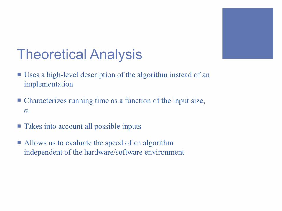
Theoretical Analysis ¡ Uses a high-level description of the algorithm instead of an

implementation

¡  Characterizes running time as a function of the input size, n.

¡  Takes into account all possible inputs

¡ Allows us to evaluate the speed of an algorithm independent of the hardware/software environment

Pseudo code ¡ High-level description of an algorithm

¡ More structured than English prose

¡  Less detailed than a program

¡  Preferred notation for describing algorithms

¡ Hides program design issues

Algorithm arrayMax(A, n) Input array A of n integers Output the maximum element of A

currentMax ← A[0] for i ← 1 to n - 1 do if A[i] > currentMax then currentMax ← A[i] return currentMax

Example: find the max element of an array

Pseudo code

Algorithm arrayMax(A, n) Input array A of n integers Output the maximum element of A

currentMax ← A[0] for i ← 1 to n - 1 do if A[i] > currentMax then currentMax ← A[i] return currentMax

Example: find the max element of an array

Algorithm arrayMin(A, n) Input array A of n integers Output the minimum element of A

currentMin ← A[0] for i ← 1 to n - 1 do if A[i] < currentMin then currentMin ← A[i] return currentMin

Find the min element of an array

Pseudo code

Algorithm arraySum(A, n) Input array A of n integers Output sum of all the elements of A

currentSum ← 0 for i ← 0 to n - 1 do currentSum ← currentSum+A[i] return currentSum

Sum all the elements of an array

Algorithm arrayMin(A, n) Input array A of n integers Output the minimum element of A

currentMin ← A[0] for i ← 1 to n - 1 do if A[i] < currentMin then currentMin ← A[i] return currentMin

Find the min element of an array

Pseudo code

Algorithm arrayMultiply(A, n) Input array A of n integers Output Multiply all the elements of A

current ← 1 for i ← 0 to n - 1 do current ← current*A[i] return current

Multiply all the elements of an array

Algorithm arraySum(A, n) Input array A of n integers Output sum of all the elements of A

currentSum ← 0 for i ← 0 to n - 1 do currentSum ← currentSum+A[i] return currentSum

Sum all the elements of an array

Pseudo code Details ¡  Control flow ¡  if … then … [else …] ¡ while … do … ¡  repeat … until … ¡  for … do … ¡  Indentation replaces braces

¡ Method declaration Algorithm method (arg [, arg…])

Input … Output …

Pseudo code Details ¡ Method call

var.method (arg [, arg…])

¡  Return value return expression

¡  Expressions ← Assignment

(like = in Java) =  Equality testing

(like == in Java) n2 Superscripts and other mathematical formatting allowed

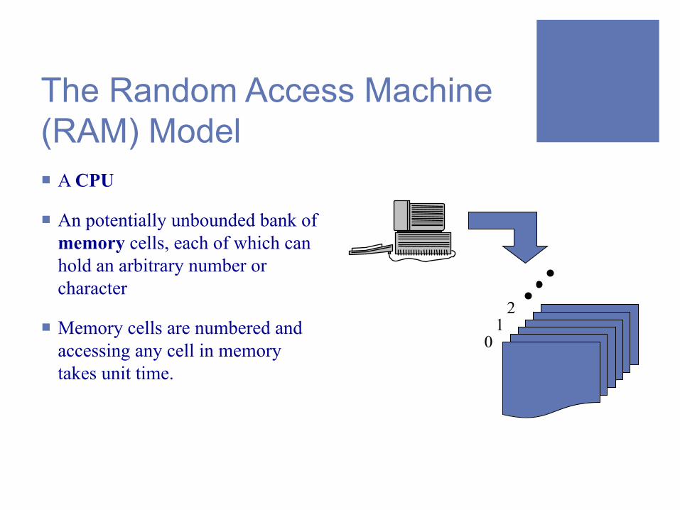
The Random Access Machine (RAM) Model ¡ A CPU

¡ An potentially unbounded bank of memory cells, each of which can hold an arbitrary number or character

¡ Memory cells are numbered and accessing any cell in memory takes unit time.

0 1

2

Seven Important Functions ¡  Seven functions that often appear in algorithm analysis: ¡  Constant ≈ 1 ¡  Logarithmic ≈ log n ¡  Linear ≈ n ¡  N-Log-N ≈ n log n ¡  Quadratic ≈ n2

¡  Cubic ≈ n3

¡  Exponential ≈ 2n

Functions Graphed Using “Normal” Scale

g(n) = 1

g(n) = lg n

g(n) = n

g(n) = 2n g(n) = n2

g(n) = n3

g(n) = n lg n

Primitive Operations ¡ Basic computations performed by an algorithm

¡  Identifiable in pseudocode

¡ Largely independent from the programming language

¡ Exact definition not important (we will see why later)

¡ Assumed to take a constant amount of time in the RAM model ¡  Examples:

¡  Evaluating an expression ¡  Assigning a value to a variable ¡  Indexing into an array ¡  Calling a method ¡  Returning from a method

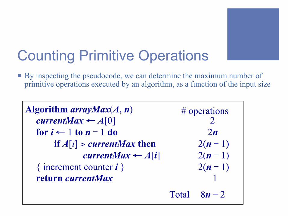
Counting Primitive Operations ¡  By inspecting the pseudocode, we can determine the maximum number of

primitive operations executed by an algorithm, as a function of the input size

Algorithm arrayMax(A, n) # operations currentMax ← A[0] 2 for i ← 1 to n - 1 do 2n if A[i] > currentMax then 2(n - 1) currentMax ← A[i] 2(n - 1) { increment counter i } 2(n - 1) return currentMax 1

Total 8n - 2

Counting Primitive Operations ¡  By inspecting the pseudocode, we can determine the maximum number of

primitive operations executed by an algorithm, as a function of the input size

Algorithm arrayMultiply(A, n) #operations current ← 1 1 for i ← 0 to n - 1 do 2(n+1) current ← current*A[i] 3n

{ increment counter i } 2n return current 1

Total 7n+4 =>O(n)

Counting Primitive Operations ¡  By inspecting the pseudocode, we can determine the maximum number of

primitive operations executed by an algorithm, as a function of the input size

Algorithm arrayAverage(A, n) #operations current ← 0 1 for i ← 0 to n - 1 do 2(n+1) current ← current+A[i] 3n

{ increment counter i } 2n return current/n 2

Total 7n+5 =>O(n)

Estimating Running Time ¡ Algorithm arrayMax executes 8n - 2 primitive operations

in the worst case. Define: a = Time taken by the fastest primitive operation b = Time taken by the slowest primitive operation

¡  Let T(n) be worst-case time of arrayMax. Then a (8n - 2) ≤ T(n) ≤ b(8n - 2)

¡ Hence, the running time T(n) is bounded by two linear functions

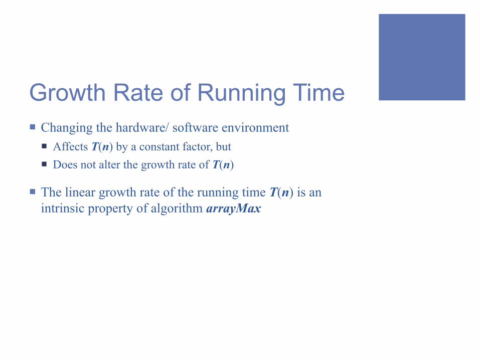
Growth Rate of Running Time ¡  Changing the hardware/ software environment ¡  Affects T(n) by a constant factor, but ¡  Does not alter the growth rate of T(n)

¡  The linear growth rate of the running time T(n) is an intrinsic property of algorithm arrayMax

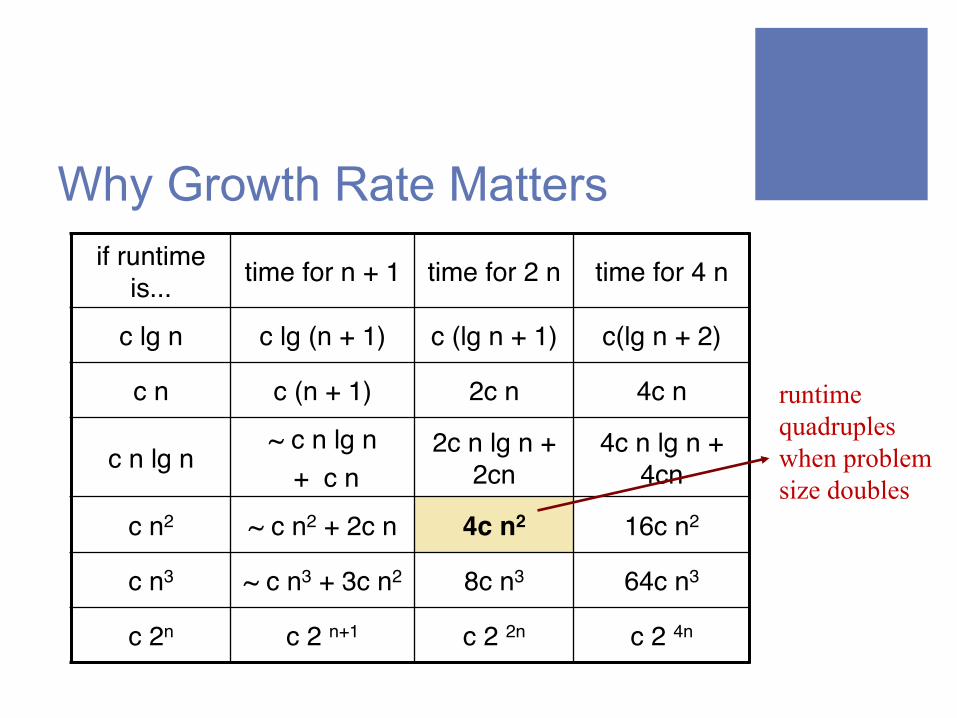
Why Growth Rate Matters

if runtime is..." time for n + 1" time for 2 n" time for 4 n"

c lg n" c lg (n + 1)" c (lg n + 1)" c(lg n + 2)"

c n" c (n + 1)" 2c n" 4c n"

c n lg n"~ c n lg n"

+ c n"2c n lg n +

2cn"4c n lg n +

4cn"

c n2" ~ c n2 + 2c n" 4c n2! 16c n2"

c n3" ~ c n3 + 3c n2" 8c n3 " 64c n3"

c 2n" c 2 n+1" c 2 2n" c 2 4n"

runtime quadruples when problem size doubles

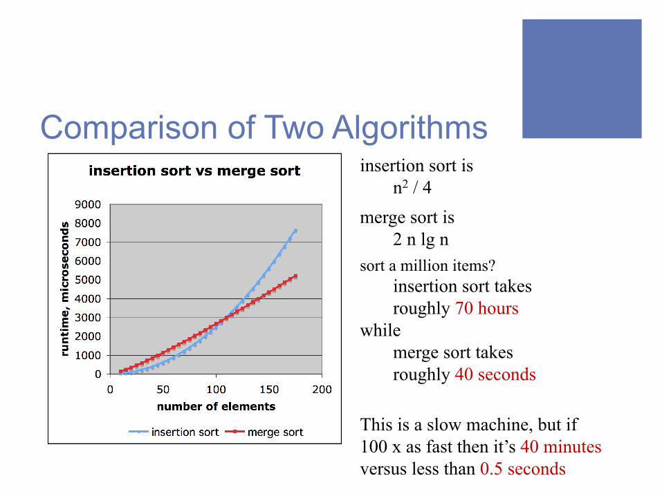
Comparison of Two Algorithms

insertion sort is n2 / 4

merge sort is 2 n lg n

sort a million items? insertion sort takes

roughly 70 hours while

merge sort takes roughly 40 seconds

This is a slow machine, but if 100 x as fast then it’s 40 minutes versus less than 0.5 seconds

Constant Factors ¡  The growth rate is not affected

by ¡  constant factors or ¡  lower-order terms

¡  Examples ¡  102n + 105 is a linear function ¡  105n2 + 108n is a quadratic

function

1E-1 1E+1 1E+3 1E+5 1E+7 1E+9

1E+11 1E+13 1E+15 1E+17 1E+19 1E+21 1E+23 1E+25

1E-1 1E+1 1E+3 1E+5 1E+7 1E+9

T(n)

n

Quadratic Quadratic Linear Linear

Big-Oh Notation ¡ Given functions f(n) and g(n),

we say that f(n) is O(g(n)) if there are positive constants c and n0 such that

f(n) ≤ cg(n) for n ≥ n0

¡  Example: 2n + 10 is O(n) ¡  2n + 10 ≤ cn ¡  (c - 2) n ≥ 10 ¡  n ≥ 10/(c - 2) ¡  Pick c = 3 and n0 = 10 1

10

100

1,000

10,000

1 10 100 1,000 n

3n

2n+10

n

Big-Oh Example ¡  Example: the function n2

is not O(n) ¡  n2 ≤ cn ¡  n ≤ c ¡  The above inequality

cannot be satisfied since c must be a constant

1

10

100

1,000

10,000

100,000

1,000,000

1 10 100 1,000 n

n^2

100n

10n

n

More Big-Oh Example ¡  7n-2 is O(n)

¡  need c > 0 and n0 ≥ 1 such that 7n-2 ≤ c•n for n ≥ n0 ¡  this is true for c = 7 and n0 = 1

¡  3n3 + 20n2 + 5 is O(n3) ¡  need c > 0 and n0 ≥ 1 such that 3n3 + 20n2 + 5 ≤ c•n3 for n ≥ n0 ¡  this is true for c = 4 and n0 = 21

¡  3 log n + 5 is O(log n) ¡  need c > 0 and n0 ≥ 1 such that 3 log n + 5 ≤ c•log n for n ≥ n0 ¡  this is true for c = 8 and n0 = 2

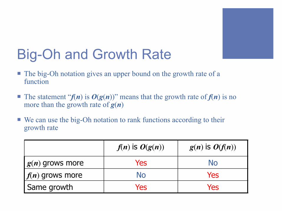
Big-Oh and Growth Rate ¡  The big-Oh notation gives an upper bound on the growth rate of a

function

¡  The statement “f(n) is O(g(n))” means that the growth rate of f(n) is no more than the growth rate of g(n)

¡  We can use the big-Oh notation to rank functions according to their growth rate

f(n) is O(g(n)) g(n) is O(f(n))

g(n) grows more Yes No

f(n) grows more No Yes

Same growth Yes Yes

Big-Oh Rules ¡  If f(n) is a polynomial of degree d, then f(n) is O(nd), i.e.,

1. Drop lower-order terms 2. Drop constant factors

¡ Use the smallest possible class of functions ¡  Say “2n is O(n)” instead of “2n is O(n2)”

¡ Use the simplest expression of the class ¡  Say “3n + 5 is O(n)” instead of “3n + 5 is O(3n)”

Asymptotic Algorithm Analysis ¡  The asymptotic analysis of an algorithm determines the

running time in big-Oh notation

¡  To perform the asymptotic analysis ¡  We find the worst-case number of primitive operations executed

as a function of the input size ¡  We express this function with big-Oh notation

Asymptotic Algorithm Analysis ¡  Example: ¡  We determine that algorithm arrayMax executes at most 8n - 2

primitive operations ¡  We say that algorithm arrayMax “runs in O(n) time”

¡  Since constant factors and lower-order terms are eventually dropped anyhow, we can disregard them when counting primitive operations

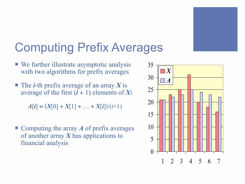
Computing Prefix Averages ¡ We further illustrate asymptotic analysis

with two algorithms for prefix averages

¡  The i-th prefix average of an array X is average of the first (i + 1) elements of X:

A[i] = (X[0] + X[1] + … + X[i])/(i+1)

¡  Computing the array A of prefix averages of another array X has applications to financial analysis

0

5

10

15

20

25

30

35

1 2 3 4 5 6 7

XA

Exercise ¡  Implement prefixAverage

¡  Input: ¡  Get n integers from a txt file ¡  The first integer indicates the number of integers

(the size of X)

¡  Output: ¡  Print out a sequence of integers ¡  The ith integer indicates the average of the first i+1 input

numbers (starting from the second input)

Input: 4 1 2 3 5

Output: 1 2 2

Prefix Average (Quadratic) ¡  The following algorithm computes prefix averages in quadratic

time by applying the definition

Algorithm prefixAverages1(X, n) Input array X of n integers Output array A of prefix averages of X #operations A ← new array of n integers n for i ← 0 to n - 1 do n s ← X[0] n for j ← 1 to i do 1 + 2 + …+ (n - 1) s ← s + X[j] 1 + 2 + …+ (n - 1) A[i] ← s / (i + 1) n return A 1

Arithmetic Progression ¡  The running time of

prefixAverages1 is O(1 + 2 + …+ n)

¡  The sum of the first n integers is n(n + 1) / 2 ¡  There is a simple visual proof of

this fact

¡  Thus, algorithm prefixAverages1 runs in O(n2) time 0

1

2

3

4

5

6

7

1 2 3 4 5 6

Prefix Average (Linear) ¡  The following algorithm computes prefix averages in linear

time by keeping a running sum

¡ Algorithm prefixAverages2 runs in O(n) time

Algorithm prefixAverages2(X, n) Input array X of n integers Output array A of prefix averages of X #operations A ← new array of n integers n s ← 0 1 for i ← 0 to n - 1 do n s ← s + X[i] n A[i] ← s / (i + 1) n return A 1

Relatives of Big-Oh ¡  big-Omega ¡  f(n) is Ω(g(n)) if there is a constant c > 0 ¡  and an integer constant n0 ≥ 1 such that ¡  f(n) ≥ c•g(n) for n ≥ n0

¡  big-Theta ¡  f(n) is Θ(g(n)) if there are constants c’ > 0 and c’’ > 0 and an

integer constant n0 ≥ 1 such that c’•g(n) ≤ f(n) ≤ c’’•g(n) for n ≥ n0

Intuition for Asymptotic Notation ¡  Big-Oh ¡  f(n) is O(g(n)) if f(n) is asymptotically less than or equal to g

(n) ¡  big-Omega ¡  f(n) is Ω(g(n)) if f(n) is asymptotically greater than or equal

to g(n)

¡  big-Theta ¡  f(n) is Θ(g(n)) if f(n) is asymptotically equal to g(n)

Examples of Using Relatives of Big-Oh ¡  5n2 is Ω(n2)

¡  f(n) is Ω(g(n)) if there is a constant c > 0 and an integer constant n0 ≥ 1 such that f(n) ≥ c•g(n) for n ≥ n0

¡  let c = 5 and n0 = 1

¡  5n2 is Ω(n) ¡  f(n) is Ω(g(n)) if there is a constant c > 0 and an integer constant n0 ≥ 1

such that f(n) ≥ c•g(n) for n ≥ n0

¡  let c = 1 and n0 = 1

¡  5n2 is Θ(n2) ¡  f(n) is Θ(g(n)) if it is Ω(n2) and O(n2). We have already seen the former,

for the latter recall that f(n) is O(g(n)) if there is a constant c > 0 and an integer constant n0 ≥ 1 such that f(n) < c•g(n) for n ≥ n0

¡  Let c = 5 and n0 = 1

Coming Up… ¡  For more about Big O: Read Text Book 4

¡ Next week we will talk about “Divide and Conquer/Sorting”: Read Text Book 11

¡ We will have the midterm exam on Dec. 2