data mining techniques1 mining frequent patterns, associations

Data Mining Techniques 1

Mining Frequent Patterns, Associations


Outline

• What is association rule mining and frequent pattern mining?

• Methods for frequent-pattern mining • Constraint-based frequent-pattern mining • Frequent-pattern mining: achievements, promise

s and research problems


Market Basket Analysis

This basket contains an assortment of products

What one customer purchased at one time???

What merchandise customers are buying and when???

Marketing basket analysis is a process that analyzes customer buying habits


What Market Basket Analysis Can Help?• Customer: who they are? why they make certain

purchase?• Merchandise: which products tend to be

purchased together? Which are most amenable to promotion? Does a brand of products make a difference?

• Usage:– Store layout;– Product layout;– Coupons issue;


Association Rules from Market Basket Analysis

Method:Transaction 1: Frozen pizza, cola, milk Transaction 2: Milk, potato chips Transaction 3: Cola, frozen pizza Transaction 4: Milk, pretzels

Transaction 5: Cola, pretzels

Frozen

PizzaMil

kCol

aPotato Chips

Pretzels

Frozen Pizza 2 1 2 0 0

Milk 1 3 1 1 1

Cola 2 1 3 0 1

Potato Chips 0 1 0 1 0

Pretzels 0 1 1 0 2

Hints that frozen pizza and cola may sell well together, and should be placed side-by-side in the convenience store..

Results:

we could derive the association rules: If a customer purchases Frozen Pizza, then they will probably purchase Cola. If a customer purchases Cola, then they will probably purchase Frozen Pizza.


Use of Rule Associations

• Coupons, discounts– Don’t give discounts on 2 items that are frequently bought

together. Use the discount on 1 to “pull” the other

• Product placement– Offer correlated products to the customer at the same time.

Increases sales

• Timing of cross-marketing– Send camcorder offer to VCR purchasers 2-3 months after VCR

purchase

• Discovery of patterns– People who bought X, Y and Z (but not any pair) bought W over

half the time


What are Frequent Patterns?

• Frequent patterns: patterns (itemsets, subsequences, substructures, etc.) that occur frequently in a database [AIS93]For example:– A set of items, such as milk and bread, that appear freq

uently together in a transaction data set is a frequent itemset

– A subsequence, such as buying first a PC, then a digital camera, and then a memory card, if it occurs frequently in a shopping history database, is a frequent sequential pattern

– A substructure, can refer to different structural forms, such as subgraph, subtree, or sublattics


Motivation

• Frequent pattern mining: finding regularities in data– What products were often purchased together? –beer

and diapers?!– What are the subsequent purchases after buying a PC?– What kinds of DNA are sensitive to a new drug?– Can we automatically classify web documents based

on frequent key-word combinations?


Why Is Freq. Pattern Mining Important?• Forms the foundation for many essential data mining tasks

– Association, correlation, and causality analysis

– Sequential, structural (e.g., sub-graph) patterns

– Pattern analysis in spatiotemporal, multimedia, time-series, and stream data

– Classification: associative classification

– Cluster analysis: frequent pattern-based clustering

– Data warehousing: iceberg cube and cube-gradient

– Semantic data compression: fascicles– Broad applications: Basket data analysis, cross-marketing, catalog

design, sale campaign analysis, web log (click stream) analysis, …


A Motivating Example

• Market basket analysis (customers shopping behavior analysis) – Which groups or sets of items are customers likely to pu

rchase on a given trip of the store?

– Results can be used in plan marketing or advertising strategies, or in the design of a new catalog.

– These patterns can be presented in the form of association rules below:

• Computer antivirus_software [support=2%, confidence=60%]


Basic Concepts

• I is the set of items {i1, i2, … id}

• A transaction T is a set of items: T={ia, ib, …, it},

. Each transaction is associated with an identifier, called TID.

• D, the task-relevant data, is a set of transactions D={T1, T2, … Tn}.

• An association rule is of the form:

A B, where A ⊂ ⊂ I, B ⊂ I, and A∩B = ∅

IT


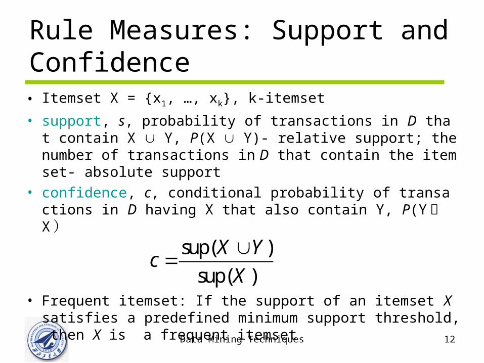
Rule Measures: Support and Confidence• Itemset X = {x1, …, xk}, k-itemset

• support, s, probability of transactions in D that contain X Y, P(X Y)- relative support; the number of transactions in D that contain the itemset- absolute support

• confidence, c, conditional probability of transactions in D having X that also contain Y, P(Y ︱ X ）

• Frequent itemset: If the support of an itemset X satisfies a predefined minimum support threshold, then X is a frequent itemset

sup( )

sup( )

X Yc

X


An Example

Customerbuys diaper

Customerbuys both

Customerbuys beer

TID Items bought

10 A, B, D

20 A, C, D

30 A, D, E

40 B, E, F

50 B, C, D, E, F

Let supmin = 50%,

confmin = 50%

Frequent patterns are:{A:3, B:3, D:4, E:3, AD:3}

Association rules:A D (60%, 100%)D A (60%, 75%)


Problem Definition

• Given I={i1, i2,…, im}, D={t1, t2, …, tn} ,and the minimum support and confidence thresholds,– frequent pattern mining problem is to find all frequent

patterns in the D– association rule mining problem is to identify all stron

g association rules X⊂Y, that must satisfy minimum support and minimum confidence


Frequent Pattern Mining: A road Map (Ⅰ)• Based on the types of values in the rule

– Boolean associations: involve associations between the presence and absence of items

• buys (x, “SQLServer”) buys (x, “DMBook”) • buys (x, “DM Software”) [0.2%, 60%]

– Quantitative associations: describe associations between quantitative items or attributes

• age (x, “30..39”) ^ income (x, “42..48K”) ⊂ buys (x, “PC”)


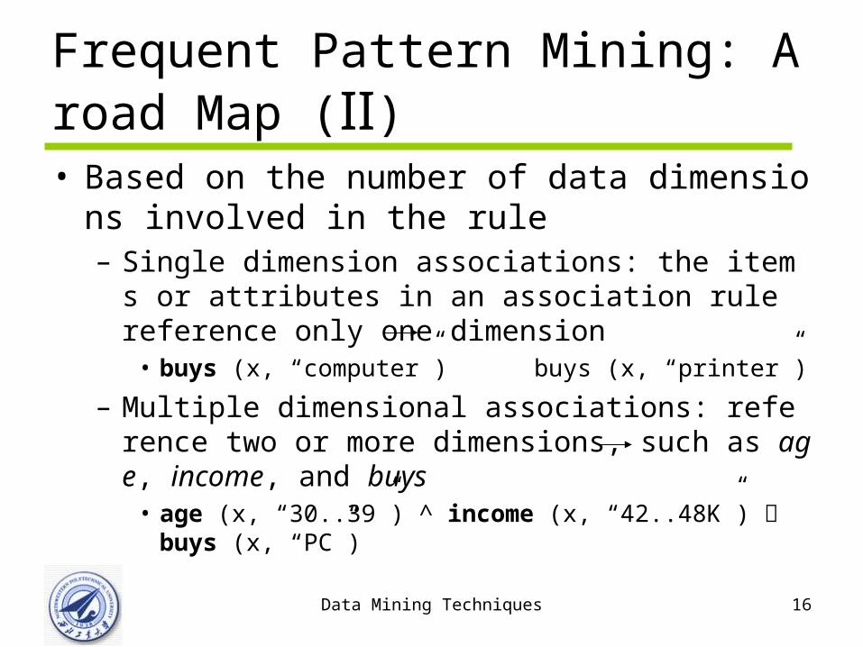
Frequent Pattern Mining: A road Map (Ⅱ)• Based on the number of data dimensions involve

d in the rule– Single dimension associations: the items or attributes

in an association rule reference only one dimension• buys (x, “computer”) buys (x, “printer”)

– Multiple dimensional associations: reference two or more dimensions, such as age, income, and buys

• age (x, “30..39”) ^ income (x, “42..48K”) ⊂ buys (x, “PC”)


Frequent Pattern Mining: A road Map (Ⅲ)• Based on the levels of abstraction involved in th

e rule set– Single level

• buys (x, “computer”) buys (x, “printer”)

– multiple-level analysis• What brands of computers are associated with what brands

of digital cameras?• buys (x, “laptop_computer”) buys (x, “HP_printer”)


Multiple-Level Association Rules

• Items often form hierarchies

TID Items Purchased

1 IBM-ThinkPad-R40/P4M, Symantec-Norton-Antivirus-2003

2 Microsoft-Office-Proffesional-2003, Microsoft-

3 logiTech-Mouse, Fellows-Wrist-Rest

… …

all

Computer Software Printer & Camera Accessory

laptop desktop office antivirus printer camera mouse pad

Level 1

Level 0

Level 2

Level 3IBM Dell Microsoft


Frequent Pattern Mining: A road Map (Ⅳ)• Based on the completeness of patterns to be min

ed– Complete set of frequent itemsets– Closed frequent itemsets– Maximal frequent itemsets– Constrained frequent itemsets– Approximate frequent itemsets– …

FrequentItemsets

ClosedFrequentItemsets

MaximalFrequentItemsets


Outline


• Methods for frequent-pattern mining • Constraint-based frequent-pattern mining • Frequent-pattern mining: achievements, promise

s and research problems


Frequent Pattern Mining Methods

• Apriori and its variations/improvements

• Mining frequent-patterns without candidate generation

• Mining max-patterns and closed itemsets

• Mining multi-dimensional, multi-level frequent patterns with flexible support constraints

• Interestingness: correlation and causality


Data Representation

• Transactional vs. Binary

• Horizontal vs. Vertical

TID Items

10 a, c, d

20 b, c, e

30 a, b, c, e

40 b, e

TID a b c d e

10 1 0 1 1 0

20 0 1 1 0 1

30 1 1 1 0 1

40 0 1 0 0 1

Item TIDs

a 10, 30

b 20, 30, 40

c 10, 20, 30

d 10

e 20, 30, 40


Apriori: A Candidate Generation-and-Test Approach

• Apriori is a seminal algorithm proposed by R.

Agrawal & R. Srikant [VLDB’94]

• Apriori consists of two phases:– Generate length (k+1) candidate itemsets from leng

th k frequent itemsets• Join step• Prune step

– Test the candidates against DB


Apriori-Based Mining

• Method:

– Initially, scan DB once to get frequent 1-itemset

– Generate length (k+1) candidate itemsets from length

k frequent itemsets

– Test the candidates against DB

– Terminate when no frequent or candidate set can be

generated


Apriori Property

• Apriori pruning property: If there is any itemset w

hich is infrequent, its superset should not be gen

erated/tested! – No superset of any infrequent itemset should be gene

rated or tested– Many item combinations can be pruned!


Illustrating Apriori Principle

Found to be Infrequent

null

AB AC AD AE BC BD BE CD CE DE

A B C D E

ABC ABD ABE ACD ACE ADE BCD BCE BDE CDE

ABCD ABCE ABDE ACDE BCDE

ABCDE

null

AB AC AD AE BC BD BE CD CE DE

A B C D E

ABC ABD ABE ACD ACE ADE BCD BCE BDE CDE

ABCD ABCE ABDE ACDE BCDE

ABCDEPruned supersets

The whole process of frequent pattern mining can be seen as a searchIn the lattice

start


Apriori Algorithm—An Example

Database TDB

1st scan

C1L1

L2

C2 C2

2nd scan

C3 L33rd scan

Tid Items

10 A, C, D

20 B, C, E

30 A, B, C, E

40 B, E

Itemset sup

{A} 2

{B} 3

{C} 3

{D} 1

{E} 3

Itemset sup

{A} 2

{B} 3

{C} 3

{E} 3

Itemset

{A, B}

{A, C}

{A, E}

{B, C}

{B, E}

{C, E}

Itemset sup{A, B} 1{A, C} 2{A, E} 1{B, C} 2{B, E} 3{C, E} 2

Itemset sup{A, C} 2{B, C} 2{B, E} 3{C, E} 2

Itemset

{B, C, E}

Itemset sup{B, C, E} 2

Supmin = 2


The Apriori Algorithm

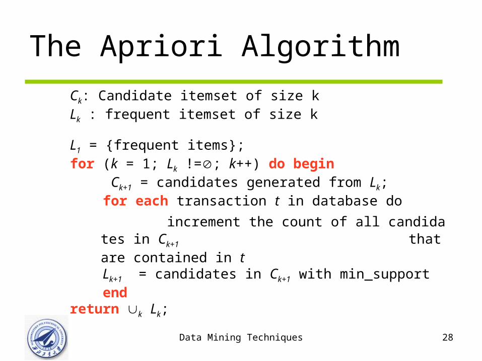
Ck: Candidate itemset of size kLk : frequent itemset of size k

L1 = {frequent items};for (k = 1; Lk !=; k++) do begin Ck+1 = candidates generated from Lk; for each transaction t in database do

increment the count of all candidates in Ck+1 that are contained in t

Lk+1 = candidates in Ck+1 with min_support endreturn k Lk;


Important Details of Apriori

• How to generate candidates?– Step 1: self-joining Lk

– Step 2: pruning

• How to count supports of candidates?


• Suppose the items in Lk-1 are listed in an order

• Step 1: self-joining Lk-1 insert into Ck

select p.item1, p.item2, …, p.itemk-1, q.itemk-1

from Lk-1 p, Lk-1 q

where p.item1=q.item1, …, p.itemk-2=q.itemk-2, p.itemk-1 < q.itemk-1

• Step 2: pruningforall itemsets c in Ck do

forall (k-1)-subsets s of c do

if (s is not in Lk-1) then delete c from Ck

How to Generate Candidates?


• Why counting supports of candidates a problem?– The total number of candidates can be very huge

– One transaction may contain many candidates

• Method:– Candidate itemsets are stored in a hash-tree

– Leaf node of hash-tree contains a list of itemsets and counts

– Interior node contains a hash table

– Subset function: finds all the candidates contained in a transaction

How to Count Supports of Candidates?


Counting Supports of Candidates Using Hash Tree

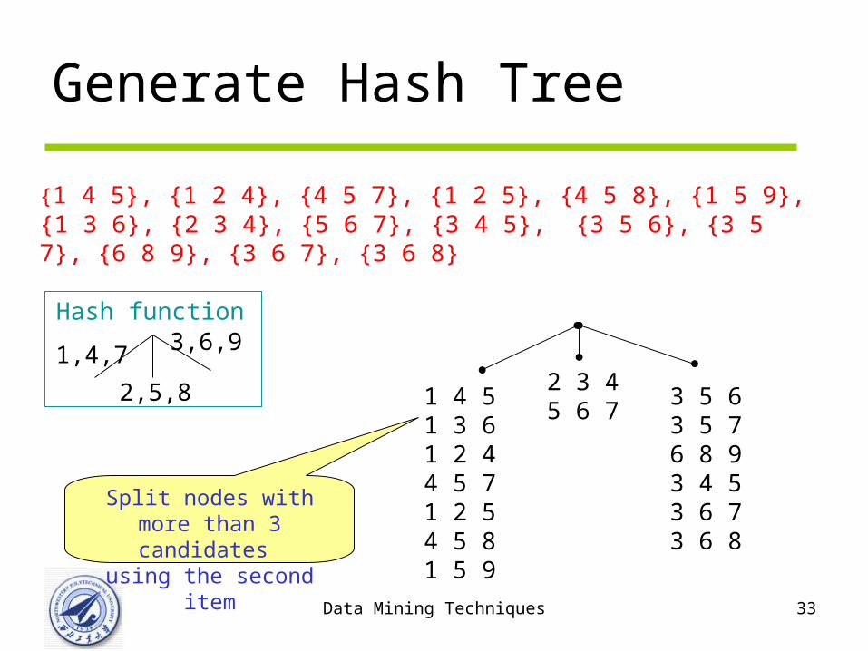
• Suppose you have 15 candidate itemsets of length 3: {1 4 5}, {1 2 4}, {4 5 7}, {1 2 5}, {4 5 8}, {1 5 9}, {1 3 6}, {2 3 4}, {5 6 7}, {3 4 5}, {3 5 6}, {3 5 7}, {6 8 9}, {3 6 7}, {3 6 8}

• You need:– Hash function – Max leaf size: max number of itemsets stored in a lea

f node (if number of candidate itemsets exceeds max leaf size, split the node)


1,4,7

2,5,8

3,6,9Hash function

{1 4 5}, {1 2 4}, {4 5 7}, {1 2 5}, {4 5 8}, {1 5 9}, {1 3 6}, {2 3 4}, {5 6 7}, {3 4 5}, {3 5 6}, {3 5 7}, {6 8 9}, {3 6 7}, {3 6 8}

2 3 45 6 7

1 4 51 3 61 2 44 5 71 2 54 5 81 5 9

3 5 63 5 76 8 93 4 53 6 73 6 8

Split nodes with more than 3 candidates

using the second item

Generate Hash Tree


1,4,7

2,5,8

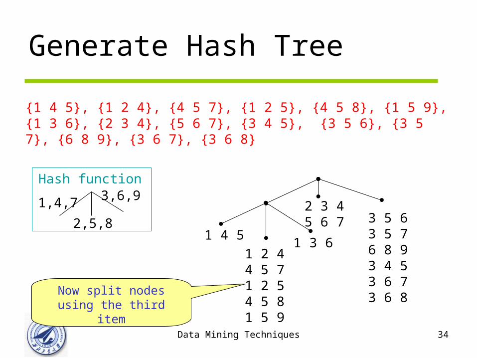
3,6,9Hash function

{1 4 5}, {1 2 4}, {4 5 7}, {1 2 5}, {4 5 8}, {1 5 9}, {1 3 6}, {2 3 4}, {5 6 7}, {3 4 5}, {3 5 6}, {3 5 7}, {6 8 9}, {3 6 7}, {3 6 8}

2 3 45 6 7 3 5 6

3 5 76 8 93 4 53 6 73 6 8

1 2 44 5 71 2 54 5 81 5 9

1 4 51 3 6

Now split nodesusing the third item

Generate Hash Tree


1,4,7

2,5,8

3,6,9Hash function

{1 4 5}, {1 2 4}, {4 5 7}, {1 2 5}, {4 5 8}, {1 5 9}, {1 3 6}, {2 3 4}, {5 6 7}, {3 4 5}, {3 5 6}, {3 5 7}, {6 8 9}, {3 6 7}, {3 6 8}

2 3 45 6 7 3 5 6

3 5 76 8 93 4 53 6 73 6 8

1 4 51 3 6

1 2 44 5 7 1 2 5

4 5 81 5 9

Now, split this similarly.

Generate Hash Tree


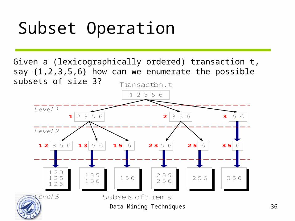
Subset Operation

1 2 3 5 6

Transaction, t

2 3 5 61 3 5 62

5 61 33 5 61 2 61 5 5 62 3 62 5

5 63

1 2 31 2 51 2 6

1 3 51 3 6

1 5 62 3 52 3 6

2 5 6 3 5 6

Subsets of 3 items

Level 1

Level 2

Level 3

63 5

Given a (lexicographically ordered) transaction t, say {1,2,3,5,6} how can we enumerate the possible subsets of size 3?


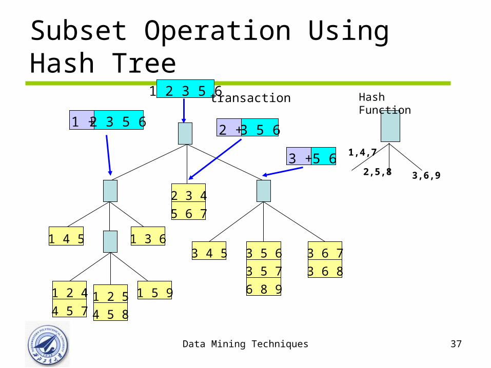
Subset Operation Using Hash Tree

1 5 9

1 4 5 1 3 63 4 5 3 6 7

3 6 8

3 5 6

3 5 7

6 8 9

2 3 4

5 6 7

1 2 4

4 5 71 2 5

4 5 8

1 2 3 5 6

1 + 2 3 5 63 5 62 +

5 63 +1,4,7

2,5,8 3,6,9

Hash Functiontransaction



1 5 9

1 4 5 1 3 63 4 5 3 6 7

3 6 8

3 5 6

3 5 7

6 8 9

2 3 4

5 6 7

1 2 4

4 5 71 2 5

4 5 8

1,4,7

2,5,8

3,6,9

Hash Function1 2 3 5 6

3 5 61 2 +

5 61 3 +

61 5 +

3 5 62 +

5 63 +

1 + 2 3 5 6

transaction



1 5 9

1 4 5 1 3 63 4 5 3 6 7

3 6 8

3 5 6

3 5 7

6 8 9

2 3 4

5 6 7

1 2 4

4 5 71 2 5

4 5 8

1,4,7

2,5,8

3,6,9

Hash Function1 2 3 5 6

3 5 61 2 +

5 61 3 +

61 5 +

3 5 62 +

5 63 +

1 + 2 3 5 6

transaction

Match transaction against 11 out of 15 candidates


How the Hash Tree Works

• Suppose t = {1, 2, 3, 4, 5}• First all size 3-itemsets must begin with 1, 2 or 3• Therfore at the root must hash on 1, 2 and 3 sep

arately• Once we reach the child of the root, need to has

h again repeat the process till the algorithm reaches the leaves check if each candidate in the leaf is a subset of the transaction and increment count if it is In the example, 6/9 leaf nodes are visited and 11/15 itemsets are matched


Generating Association Rules From Frequent Itemsets• For each frequent itemset l, generate all nonempty

subset of l

• For every nonempty subset s of l, output the rule

– Example: Suppose l = {I1, I2, I5}. The nonempty subsets of l are

{I1,I2} ,{I1,I5},{I2,I5},{I1},{I2},and{I5}. The association rules are:

I1∧I2 I5 c=2/4=50% I1∧I5 I2 c=2/2=100% I2∧I5 I5 c=2/2=100%

I1 I2∧I5 c=2/6=33% I2 I1∧I5 c=2/7=29% I5 I1∧I2 c=2/2=100%

sup_ ( )

sup_ ( )

count A Bc

count A

sup_ ( )

sup_ ( )

count l

count s

TID Item_IDs

T10 I1,I2,I5

T20 I2,I4

T30 I2,I3

T40 I1,I2,I4

T50 I1,I3

T60 I2,I3

T70 I1,I3

T80 I1,I2,I3,I5

T90 I1,I2,I3


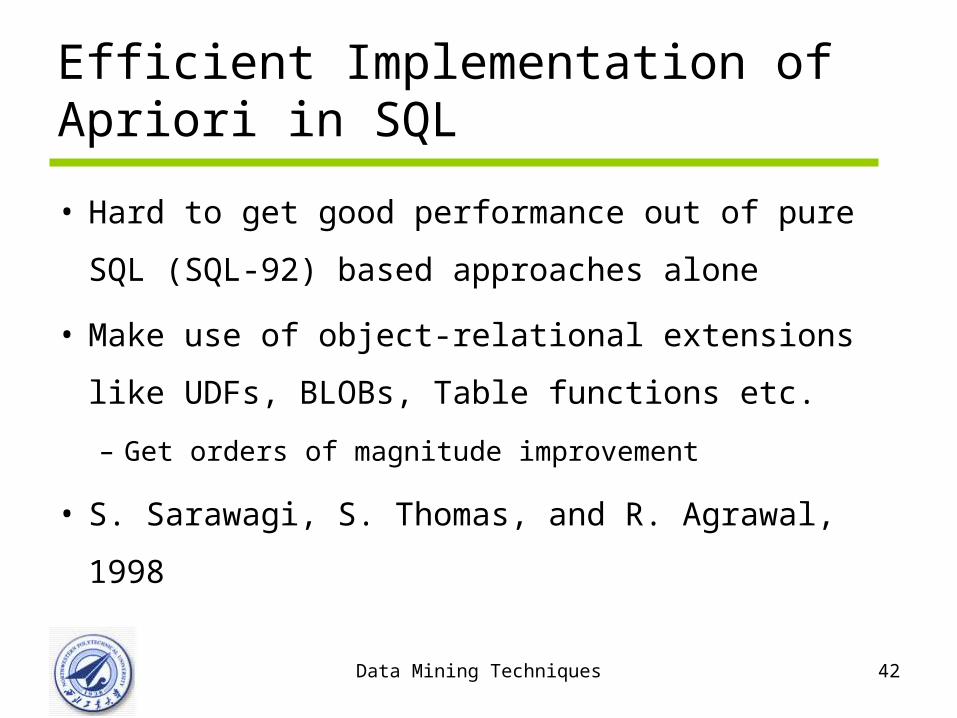
Efficient Implementation of Apriori in SQL

• Hard to get good performance out of pure SQL

(SQL-92) based approaches alone

• Make use of object-relational extensions like U

DFs, BLOBs, Table functions etc.

– Get orders of magnitude improvement

• S. Sarawagi, S. Thomas, and R. Agrawal, 1998


Challenges of Frequent Itemset Mining• The core of the Apriori algorithm

– Use frequent (k–1)-itemsets to generate candidate frequent k-itemsets

– Use database scan to collect counts for the candidate itemsets• Challenge

– Multiple scans of transaction database-costly

• Needs (n +1 ) scans, n is the length of the longest pattern

– Huge number of candidates especially when support threshold is s

et low• 104 frequent 1-itemset will generate 107 candidate 2-itemsets• To discover a frequent pattern of size 100, e.g., {a1, a2, …, a100}, one n

eeds to generate 2100 ~ 1030 candidates.

– Tedious workload of support counting for candidates


Outline

• Methods for improving Apriori

• An interesting approach – FP-growth


Methods to Improve Apriori’s Efficiency

• Improving Apriori: general ideas

– Reduce passes of transaction database scans

– Shrink number of candidates

– Facilitate support counting of candidates


DIC: Reduce Number of Scans

• DIC (Dynamic Itemset Counting ): tries to reduce the number of passes over the database by dividing the database into intervals of a specific size

• Intuitively, DIC works like a train running over the data with stops at intervals M transactions apart (M is a parameter)

• S. Brin R. Motwani, J. Ullman, and S. Tsur. “Dynamic itemset counting and implication rules for market basket data”. In SIGMOD’97


DIC: Reduce Number of Scans

ABCD

ABC ABD ACD BCD

AB AC BC AD BD CD

A B C D

{}

Itemset lattice

• Candidate 1-itemsets are generated • Once both A and D are determined frequent, the counting of AD begins• Once all length-2 subsets of BCD are determined frequent, the

counting of BCD begins

Transactions

1-itemsets2-itemsets

…Apriori

1-itemsets2-items

3-itemsDIC


DIC: An Example

• A transaction database TDB with 40,000 transactions; support threshold=100; M =10,000– If itemset a and b get support counts greater than 100 in the first 10,000 tra

nsactions, DIC will start counting 2-itemset ab after the first 10,000 transactions

– Similarly, if ab, ac and bc are contained in at least 100 transactions among the second 10,000 transactions, DIC will start counting 3-itemset abc after 20,000 transactions

– Once DIC gets to the end of the transaction database TDB, it will stop counting the 1-itemsets and go back to the start of the database and count the 2 and 3-itemsets

– After the first 10,000 transactions, DIC will finish counting ab, and after 20,000 transactions, it will finish counting abc

By overlapping the counting of different lengths of itemsets, DIC can save some database scans


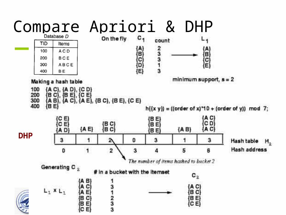
DHP: Reduce the Number of Candidates

• DHP (Direct Hashing and Pruning ): reduces the n

umber of candidate itemsets

• J. Park, M. Chen, and P. Yu. “An effective hash-b

ased algorithm for mining association rules”. In SI

GMOD’95


DHP: Reduce the Number of Candidates• In the k-th scan, DHP counts not only length-k can

didates, but also buckets of length-(k+1) potential candidates

• A k-itemset whose corresponding hashing bucket

count is below the threshold cannot be frequent– Candidates: a, b, c, d, e

– Hash entries: {ab, ad, ae} {bd, be, de} …

– Frequent 1-itemset: a, b, d, e

– ab is not a candidate 2-itemset if the sum of count of {ab, ad, ae} is

below support threshold


Compare Apriori & DHP

DHP


DHP: Database Trimming


Example: DHP


Partition: A Two Scan Method

• Partition: requires just two database scans to mine the frequent itemsets

• A. Savasere, E. Omiecinski, and S. Navathe, “An efficient algorithm for mining association rules in large databases”. VLDB’95


A Two Scan Method: Partition

• Partition the database into n partitions, such that

each partition can be held into main memory• Itemset X is frequent ⊂X must be frequent in at

least one partition– Scan 1: partition database and find local frequent patt

erns– Scan 2: consolidate global frequent patterns

• All local frequent itemsetscan be held in main

memory? A sometimes too strong assumption


Partitioning


Sampling for Frequent Patterns

• Sampling : selects a sample of original database,

mine frequent patterns within sample using Apriori

• H. Toivonen. “Sampling large databases for associ

ation rules”. In VLDB’96


Sampling for Frequent Patterns

• Scan database once to verify frequent itemsets fo

und in sample, only borders of closure of frequent

patterns are checked

– Example: check abcd instead of ab, ac, …, etc.

• Scan database again to find missed frequent patt

erns

• Trade off some degree of accuracy against efficie

ncy


Eclat

• Eclat: uses the vertical database layout and uses the intersection based approach to compute the support of an itemset

• H. Toivonen. “Sampling large databases for associ

ation rules”. In VLDB’96


Eclat – An Example

• Transform the horizontally formatted data to the vertical format

TID Item_IDs

T10 I1,I2,I5

T20 I2,I4

T30 I2,I3

T40 I1,I2,I4

T50 I1,I3

T60 I2,I3

T70 I1,I3

T80 I1,I2,I3,I5

T90 I1,I2,I3

HorizontalData Layout Vertical Data Layout

Itemset TID_set

I1 {T10, T40, T50, T70, T80, T90}

I2 {T10, T20, T30, T40, T60, T80, T90}

I3 {T30, T50, T60, T70, T80, T90}

I4 {T20, T40}

I5 {T10, T80}


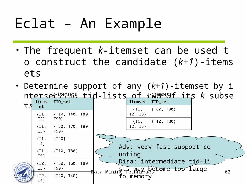
Eclat – An Example

• The frequent k-itemset can be used to construct the candidate (k+1)-itemsets

• Determine support of any (k+1)-itemset by intersecting tid-lists of two of its k subsets

Itemset TID_set

{I1, I2} {T10, T40, T80, T90}

{I1, I3} {T50, T70, T80, T90}

{I1, I4} {T40}

{I1, I5} {T10, T80}

{I2, I3} {T30, T60, T80, T90}

{I2, I4} {T20, T40}

{I2, I5} {T10, T80}

{I3, I5} {T80}

2-itemsets

Itemset TID_set

{I1, I2, I3} {T80, T90}

{I1, I2, I5} {T10, T80}

3-itemsets

Adv: very fast support countingDisa: intermediate tid-lists may become too large fo memory


Apriori-like Advantage

• Uses large itemset property

• Easily parallelized

• Easy to implement


Apriori-Like Bottleneck

• Multiple database scans are costly

• Mining long patterns needs many passes of scanning and generates lots of candidates

– To find frequent itemset i1i2…i100

• # of scans: 100

• # of Candidates: (1001) + (100

2) + … + (11

00

00) = 2100-1 =

1.27*1030 !

• Bottleneck: candidate-generation-and-test

• Can we avoid candidate generation?


Mining Frequent Patterns Without Candidate Generation

• Grow long patterns from short ones using lo

cal frequent items

– “abc” is a frequent pattern

– Get all transactions having “abc”: DB|abc

– “d” is a local frequent item in DB|abc abcd is

a frequent pattern


Compress Database by FP-tree

{}

f:1

c:1

a:1

m:1

p:1

Header Table

Item frequency head f 4c 4a 3b 3m 3p 3

min_support = 3

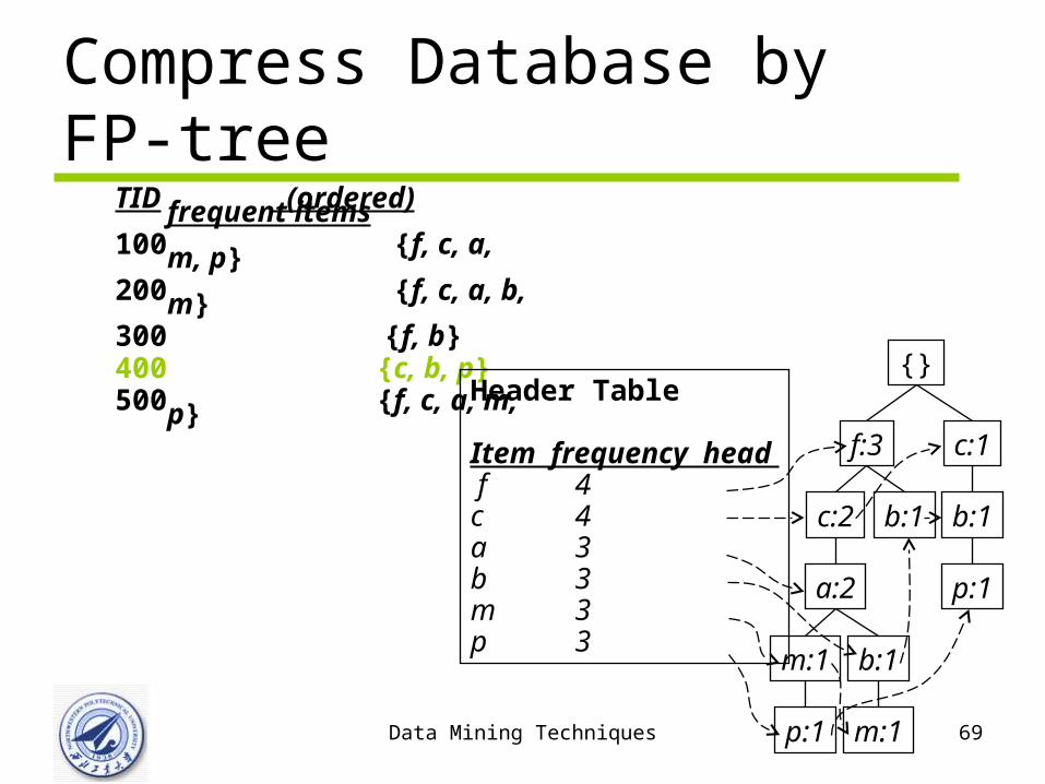
TID Items bought (ordered) frequent items100 {f, a, c, d, g, i, m, p} {f, c, a, m, p}200 {a, b, c, f, l, m, o} {f, c, a, b, m}300 {b, f, h, j, o, w} {f, b}400 {b, c, k, s, p} {c, b, p}500 {a, f, c, e, l, p, m, n} {f, c, a, m, p}

1. Scan DB once, find frequent 1-itemset (single item pattern)

2. Sort frequent items in frequency descending order, L-list

3. Scan DB again, construct FP-tree

F-list=f-c-a-b-m-p


Compress Database by FP-tree

{}

f:2

c:2

a:2

b:1m:1

p:1 m:1

Header Table


TID (ordered) frequent items100 {f, c, a, m, p}200 {f, c, a, b, m}300 {f, b}400 {c, b, p}500 {f, c, a, m, p}


Compress Database by FP-treeTID (ordered) frequent items100 {f, c, a, m, p}200 {f, c, a, b, m}300 {f, b}400 {c, b, p}500 {f, c, a, m, p} {}

f:3

b:1c:3

a:3

b:1m:2

p:2 m:1

Header Table




f:3 c:1

b:1

p:1

b:1c:2

a:2

b:1m:1

p:1 m:1

Header Table




f:4 c:1

b:1

p:1

b:1c:3

a:3

b:1m:2

p:2 m:1

Header Table



Benefits of the FP-tree

• Completeness – Preserve complete information for frequent pattern

mining– Never break a long pattern of any transaction

• Compactness– Reduce irrelevant info—infrequent items are gone– Items in frequency descending order: the more

frequently occurring, the more likely to be shared– Never be larger than the original database (not count

node-links and the count field)– For Connect-4 DB, compression ratio could be over 100


Partition Patterns and Databases• Frequent patterns can be partitioned into subset

s according to f-list: f-c-a-b-m-p– Patterns containing p– Patterns having m but no p– …– Patterns having c but no a nor b, m, or p– Pattern f

• The partitioning is complete and does not have any overlap


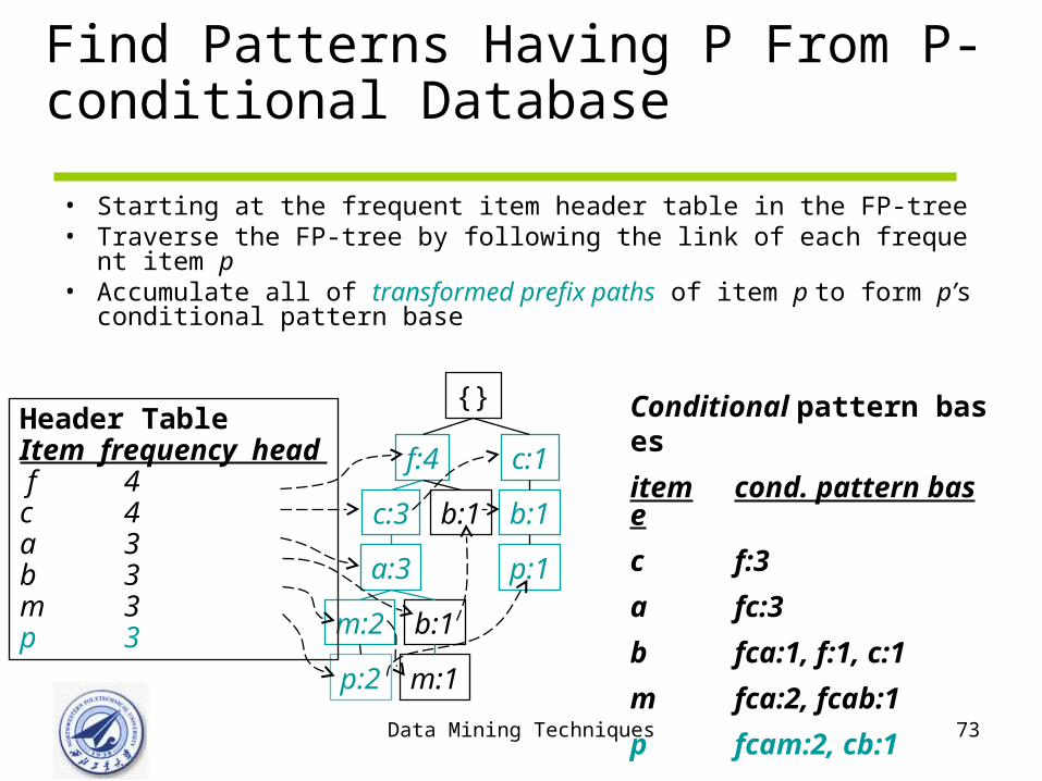
Find Patterns Having P From P-conditional Database

• Starting at the frequent item header table in the FP-tree• Traverse the FP-tree by following the link of each frequent item p• Accumulate all of transformed prefix paths of item p to form p’s cond

itional pattern base

Conditional pattern bases

item cond. pattern base

c f:3

a fc:3

b fca:1, f:1, c:1

m fca:2, fcab:1

p fcam:2, cb:1

{}

f:4 c:1

b:1

p:1

b:1c:3

a:3

b:1m:2

p:2 m:1

Header TableItem frequency head f 4c 4a 3b 3m 3p 3


From Conditional Pattern-bases to Conditional FP-trees

• For each pattern-base– Accumulate the count for each item in the base– Construct the FP-tree for the frequent items of the

pattern base

p-conditional pattern base:fcam:2, cb:1

{}

c:3

m-conditional FP-tree

All frequent patterns relate to p

p

pc

{}

f:4 c:1

b:1

p:1

b:1c:3

a:3

b:1m:2

p:2 m:1



Recusive Mining

• Patterns having m but no p can be mined recursively

m-conditional pattern base:fca:2, fcab:1

{}

f:3

c:3

a:3m-conditional FP-tree

All frequent patterns relate to m

m,

fm, cm, am,

fcm, fam, cam,

fcam

{}

f:4 c:1

b:1

p:1

b:1c:3

a:3

b:1m:2

p:2 m:1



Optimization

• Optimization: enumerate patterns from single-branch FP-tree– Enumerate all combination– Support = that of the last item

• m, fm, cm, am• fcm, fam, cam• fcam

{}

f:3

c:3

a:3m-conditional FP-tree


A Special Case: Single Prefix Path in FP-tree• A (projected) FP-tree has a single prefix

– Reduce the single prefix into one node– Join the mining results of the two parts

a2:n2

a3:n3

a1:n1

{}

b1:m1C1:k1

C2:k2 C3:k3

b1:m1C1:k1

C2:k2 C3:k3

r1

+a2:n2

a3:n3

a1:n1

{}

r1 =

enumeration of all the combinations of the sub-pathes of P


FP-Growth

• Idea: Frequent pattern growth– Recursively grow frequent patterns by pattern and

database partition

• Method – For each frequent item, construct its conditional

pattern-base, and then its conditional FP-tree– Repeat the process on each newly created conditional

FP-tree – Until the resulting FP-tree is empty, or it contains only

one path—single path will generate all the combinations of its sub-paths, each of which is a frequent pattern


Scaling Up FP-growth by Database Projection• What if FP-tree cannot fit in memory?—Database

projection– Partition a database into a set of projected Databases– Construct and mine FP-tree for each projected

Database• Heuristic: Projected database shrinks quickly in many

applications

– Such a process can be recursively applied to any projected database if its FP-tree still cannot fit in main memory

How?


Partition-based Projection

• Parallel projection needs a lot of disk space

• Partition projection saves it

Tran. DB fcampfcabmfbcbpfcamp

p-proj DB fcamcbfcam

m-proj DB fcabfcafca

b-proj DB fcb…

a-proj DBfc…

c-proj DBf…

f-proj DB …

am-proj DB fcfcfc

cm-proj DB fff

…


FP-Growth vs. Apriori: Scalability With the Support Threshold

0

10

20

30

40

50

60

70

80

90

100

0 0.5 1 1.5 2 2.5 3

Support threshold(%)

Ru

n t

ime

(se

c.)

D1 FP-grow th runtime

D1 Apriori runtime

Data set T25I20D10K: the average transaction size and average maximal potentially frequent

itemset size are set to 25 and 20, respectively, while the number of transactions in the dataset is set to 10K [AS94]


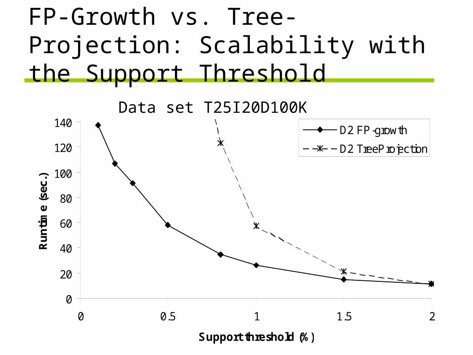
FP-Growth vs. Tree-Projection: Scalability with the Support Threshold

0

20

40

60

80

100

120

140

0 0.5 1 1.5 2

Support threshold (%)

Ru

nti

me

(sec

.)

D2 FP-growth

D2 TreeProjection

Data set T25I20D100K


Why Is FP-Growth Efficient?

• Divide-and-conquer: – decompose both the mining task and DB according to

the frequent patterns obtained so far

– leads to focused search of smaller databases

• Other factors– no candidate generation, no candidate test

– compressed database: FP-tree structure

– no repeated scan of entire database

– basic ops—counting local freq items and building sub FP-tree, no pattern search and matching


Major Costs in FP-Growth

• Poor locality of FP-trees– Low hit rate of cache

• Building FP-trees– A stack of FP-trees

• Redundant information– Transaction abcd appears in a-, ab-, abc-, ac-, …, c-p

rojected databases and FP-trees.

• Can we avoid the redundancy?


Implications of the Methodology

• Mining closed frequent itemsets and max-patterns

– CLOSET (DMKD’00)

• Constraint-based mining of frequent patterns

– Convertible constraints (KDD’00, ICDE’01)

• Computing iceberg data cubes with complex meas

ures

– H-tree and H-cubing algorithm (SIGMOD’01)


Closed Frequent Itemsets

• An itemset X is closed if none of its immediate supersets has the same support as X.

• An itemset X is not closed if at least one of its immediate supersets has the same support count as X. – For example

• Database: {(1,2,3,4),(1,2,3,4,5,6)}• Itemset (1,2) is not a closed itemset• Itemset (1,2,3,4) is a closed itemset

• An itemset is a closed frequent itemset if it is closed and its support satisfies support threshold.


Benefits of closed frequent itemsets

• It reduces redundant patterns to be generated– A frequent itemset , the total number of frequ

ent itemsets that it contains is

(1001) + (100

2) + … + (11

00

00) = 2100-1 = 1.27*1030 !

• It has the same power as frequent itemset mining• It improves not only efficiency but also

effectiveness of mining

{ }1 2 100, , ,a a a


Mining Closed Frequent Itemsets ( )Ⅰ

• Itemset merging: if Y appears in every occurrence of X, then

Y is merged with X– For example, the projected conditional database for prefix item {I5:2}

is {{I2,I1},{I2,I1,I3}}. Item {I2,I1} can be merged with {I5} to form the cl

osed itemset, {I5,I2,I1:2}

• Sub-itemset pruning: if Y כ X, and sup(X) = sup(Y), X and all

of X’s descendants in the set enumeration tree can be prune

d– For example, suppose a transaction database:

min_sup=2. The projection on the item , . Thus the mini

ng of closed frequent itemset in this data set terminates after mining

Projected database.

1 2 100 1 2 50, , , , , , ,a a a a a a

1a 1 2 50, , , : 2a a a

1' sa


Mining Closed Frequent Itemsets( )Ⅱ• Item skipping: if a local frequent item has the same suppor

t in several header tables at different levels, one can prune

it from the header table at higher levels– For example, a transaction database: , min_s

up = 2. Because in ‘s projected database has the same suppor

t as in the global header table, can be pruned from the global

header table.

• Efficient subset checking – closure checking– Superset checking: checks if this new frequent itemset is a supers

et of some already found closed itemsets with the same support

– Subset checking

1 2 100 1 2 50, , , , , , ,a a a a a a

2a 1a2a 2a


Mining Closed Frequent Itemsets

• J. Pei, J. Han & R. Mao. CLOSET: An Efficient Al

gorithm for Mining Frequent Closed Itemsets", DM

KD'00.


Maximal Frequent Itemsets

• An itemset is maximal frequent if none of its immediate supersets is fr

equent

• Despite providing a compact representation, maximal frequent itemset

s do not contain the support information of their subsets. – For example, the support of the maximal frequent itemsets

{a, c, e}, {a, d}, and {b,c,d,e} do not provide any hint about the support of their subsets.

• An additional pass over the data set is therefore needed to determine the support counts of the non maximal frequent itemsets.

• It might be desirable to have a minimal representation of frequent item

sets that preserves the support information. – Such representation is the set of the closed frequent itemsets.


Maximal vs Closed Itemsets

FrequentItemsets

ClosedFrequentItemsets

MaximalFrequentItemsets

All maximal frequent itemsets are closed because none of the maximal frequent itemsets can have the same support count as their immediate supersets.


MaxMiner: Mining Max-patterns• 1st scan: find frequent items

– A, B, C, D, E

• 2nd scan: find support for

– AB, AC, AD, AE, ABCDE

– BC, BD, BE, BCDE

– CD, CE, CDE, DE,

• Since BCDE is a max-pattern, no need to check BC

D, BDE, CDE in later scan

• R. Bayardo. Efficiently mining long patterns from dat

abases. In SIGMOD’98

Tid Items

10 A,B,C,D,E

20 B,C,D,E,

30 A,C,D,F

Potential max-

patterns


Further Improvements of Mining Methods• AFOPT (Liu, et al. [KDD’03])

– A “push-right” method for mining condensed frequent pattern (CFP) tree

• Carpenter (Pan, et al. [KDD’03])– Mine data sets with small rows but numerous columns– Construct a row-enumeration tree for efficient mining


Mining Various Kinds of Association Rules

• Mining multilevel association

• Miming multidimensional association

• Mining quantitative association

• Mining interesting correlation patterns



• Items often form hierarchies

TID Items Purchased

1 IBM-ThinkPad-R40/P4M, Symantec-Norton-Antivirus-2003

2 Microsoft-Office-Proffesional-2003, Microsoft-

3 logiTech-Mouse, Fellows-Wrist-Rest

… …

all

Computer Software Printer & Camera Accessory

laptop desktop office antivirus printer camera mouse pad

Level 1

Level 0

Level 2

Level 3IBM Dell Microsoft



• Flexible support settings – Items at the lower level are expected to have lower sup

port

• Exploration of shared multi-level mining (Agrawal & Srikant[VLB’95], Han & Fu[VLDB’95])

uniform support

Milk[support = 10%]

2% Milk [support = 6%]

Skim Milk [support = 4%]

Level 1min_sup = 5%

Level 2min_sup = 5%

Level 1min_sup = 5%

Level 2min_sup = 3%

reduced support


Multi-level Association: Redundancy Filtering• Some rules may be redundant due to “ancestor”

relationships between items.

– Example• laptop computer HP printer [support = 8%, confidence = 70%]

• IBM laptop computer HP printer [support = 2%, confidence =

72%]

• We say the first rule is an ancestor of the second

rule.

• A rule is redundant if its support is close to the

“expected” value, based on the rule’s ancestor.


Multi-Dimensional Association

• Single-dimensional rules:buys(X, “computer”) buys(X, “printer”)

• Multi-dimensional rules: 2 dimensions or predicates

– Inter-dimension assoc. rules (no repeated predicates)age(X,”19-25”) occupation(X,“student”) buys(X, “coke”)

– hybrid-dimension assoc. rules (repeated predicates)age(X,”19-25”) buys(X, “popcorn”) buys(X, “coke”)

• Categorical Attributes: finite number of possible values, no ordering among values—data cube approach

• Quantitative Attributes: numeric, implicit ordering among values—discretization, clustering, and gradient approaches


Multi-Dimensional Association

Techniques can be categorized by how

numerical attributes, such as age or salary are

treated1. Quantitative attributes are discretized using predefined c

oncept hierarchies – Static and predetermined• A concept hierarchy for income, such as “0…20k”, “21k…30k”,

and so on.

2. Quantitative attributes are discretized or clustered into “bins” based on the distribution of the data – Dynamic, referred as quantitative association rules


Quantitative Association Rules

• Proposed by Lent, Swami and Widom ICDE’97• Numeric attributes are dynamically discretized

– Such that the confidence or compactness of the rules mined is maximized

• 2-D quantitative association rules: Aquan1 Aquan2 Acat

• Example


Quantitative Association Rules

age(X,”34-35”) income(X,”30-50K”) buys(X,”high resolution TV”)

• ARCS (association rule clustering system)- Cluster adjacent association rules to form general rules using a 2-D grid– Binning: partition the ranges of quantitative attributes into intervals

• Equal-width • Equal-frequency• Clustering-based

– Finding frequent predicate sets: once the 2-D array containing the count distribution for each category is set up, it can be scaned to find the frequent predicate sets

– Clustering the associationrules


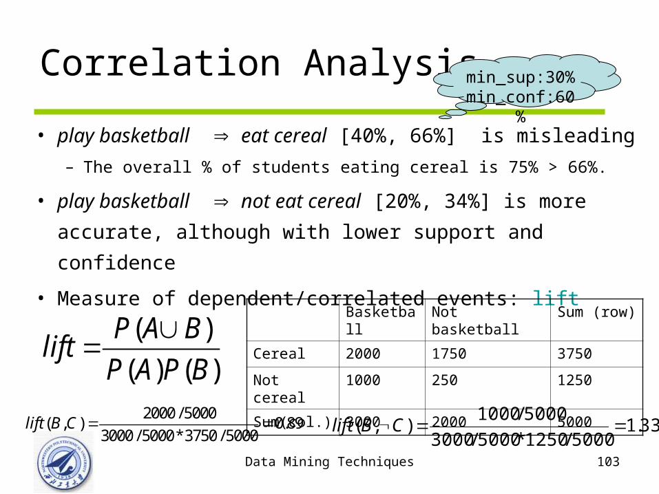
Correlation Analysis

• play basketball eat cereal [40%, 66%] is misleading

– The overall % of students eating cereal is 75% > 66%.

• play basketball not eat cereal [20%, 34%] is more

accurate, although with lower support and confidence

• Measure of dependent/correlated events: lift

2000 / 5000( , ) 0.89

3000 / 5000*3750 / 5000lift B C

Basketball Not basketball Sum (row)

Cereal 2000 1750 3750

Not cereal 1000 250 1250

Sum(col.) 3000 2000 5000

( )

( ) ( )

P A Blift

P A P B

33.15000/1250*5000/3000

5000/1000),( CBlift

min_sup:30% min_conf:60%


Outline


• Methods for frequent-pattern mining • Constraint-based frequent-pattern mining • Frequent-pattern mining: achievements, promises

and research problems


Constraint-based (Query-Directed) Mining• Finding all the patterns in a database

autonomously? — unrealistic!– The patterns could be too many but not focused!

• Data mining should be an interactive process – User directs what to be mined using a data mining query

language (or a graphical user interface)

• Constraint-based mining– User flexibility: provides constraints on what to be mined

– System optimization: explores such constraints for efficient mining—constraint-based mining


Constraints

• Constrains can be classified into five categories:– antimonotone

– Monotone

– Succinct

– Convertible

– Inconvertible


Anti-Monotone in Constraint Pushing

• Anti-monotone– When an intemset S violates the cons

traint, so does any of its superset

– sum(S.Price) v is anti-monotone

– sum(S.Price) v is not anti-monotone

• Example. C: range(S.profit) 15 is anti-monotone– Itemset ab violates C

– So does every superset of ab

TransactionTID

a, b, c, d, f10

b, c, d, f, g, h20

a, c, d, e, f30

c, e, f, g40

TDB (min_sup=2)

Item Profit

a 40

b 0

c -20

d 10

e -30

f 30

g 20

h -10


Monotone for Constraint Pushing

• Monotone

– When an intemset S satisfies the co

nstraint, so does any of its superset

– sum(S.Price) v is monotone

– min(S.Price) v is monotone

• Example. C: range(S.profit) 15

– Itemset ab satisfies C

– So does every superset of ab

TransactionTID

a, b, c, d, f10

b, c, d, f, g, h20

a, c, d, e, f30

c, e, f, g40

TDB (min_sup=2)

Item Profit

a 40

b 0

c -20

d 10

e -30

f 30

g 20

h -10


Succinctness

• Succinctness:

– Given A1, the set of items satisfying a succinctness constr

aint C, then any set S satisfying C is based on A1 , i.e., S

contains a subset belonging to A1

– Idea: Without looking at the transaction database, whethe

r an itemset S satisfies constraint C can be determined ba

sed on the selection of items

– min(S.Price) v is succinct

– sum(S.Price) v is not succinct

• Optimization: If C is succinct, C is pre-counting push

able


Converting “Tough” Constraints

• Convert tough constraints into anti-monotone or monotone by properly ordering items

• Examine C: avg(S.profit) 25– Order items in value-descending ord

er

• <a, f, g, d, b, h, c, e>

– If an itemset afb violates C

• So does afbh, afb*

• It becomes anti-monotone!

TransactionTID

a, b, c, d, f10

b, c, d, f, g, h20

a, c, d, e, f30

c, e, f, g40

TDB (min_sup=2)

Item Profit

a 40

b 0

c -20

d 10

e -30

f 30

g 20

h -10


Strongly Convertible Constraints

• avg(X) 25 is convertible anti-monotone w.r.t. item value descending order R: <a, f, g, d, b, h, c, e>– If an itemset af violates a constraint C, so does

every itemset with af as prefix, such as afd

• avg(X) 25 is convertible monotone w.r.t. item value ascending order R-1: <e, c, h, b, d, g, f, a>– If an itemset d satisfies a constraint C, so does i

temsets df and dfa, which having d as a prefix

• Thus, avg(X) 25 is strongly convertible

Item Profit

a 40

b 0

c -20

d 10

e -30

f 30

g 20

h -10


Can Apriori Handle Convertible Constraint?

• A convertible, not monotone nor anti-monotone nor succinct constraint cannot be pushed deep into the an Apriori mining algorithm– Within the level wise framework, no direct pruni

ng based on the constraint can be made

– Itemset df violates constraint C: avg(X)>=25

– Since adf satisfies C, Apriori needs df to assemble adf, df cannot be pruned

• But it can be pushed into frequent-pattern growth framework!

Item Value

a 40

b 0

c -20

d 10

e -30

f 30

g 20

h -10


Mining With Convertible Constraints

• C: avg(X) >= 25, min_sup=2

• List items in every transaction in value descending order R: <a, f, g, d, b, h, c, e>– C is convertible anti-monotone w.r.t. R

• Scan TDB once– remove infrequent items

• Item h is dropped

– Itemsets a and f are good, …

• Projection-based mining– Imposing an appropriate order on item projection

– Many tough constraints can be converted into (anti)-monotone

TransactionTID

a, f, d, b, c10

f, g, d, b, c20

a, f, d, c, e30

f, g, h, c, e40

TDB (min_sup=2)

Item Value

a 40

f 30

g 20

d 10

b 0

h -10

c -20

e -30


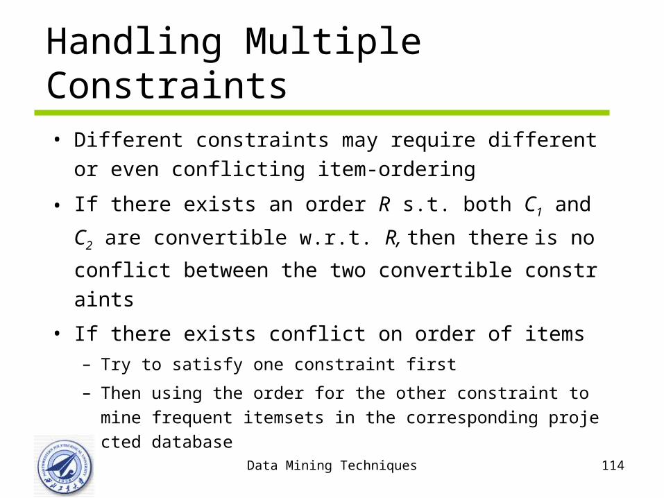
Handling Multiple Constraints

• Different constraints may require different or even con

flicting item-ordering

• If there exists an order R s.t. both C1 and C2 are conve

rtible w.r.t. R, then there is no conflict between the two

convertible constraints

• If there exists conflict on order of items– Try to satisfy one constraint first

– Then using the order for the other constraint to mine frequent

itemsets in the corresponding projected database


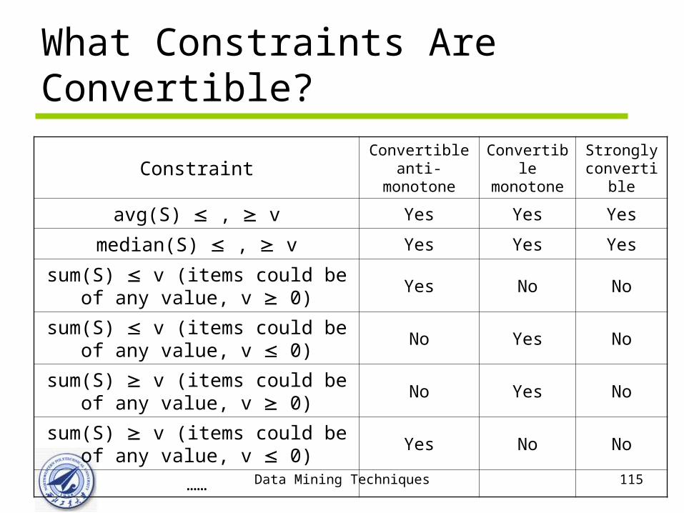
What Constraints Are Convertible?

ConstraintConvertible

anti-monotoneConvertible monotone

Strongly convertible

avg(S) , v Yes Yes Yes

median(S) , v Yes Yes Yes

sum(S) v (items could be of any value, v 0)

Yes No No


No Yes No


No Yes No


Yes No No

……


Constraint-Based Mining—A General Picture

Constraint Antimonotone Monotone Succinct

v S no yes yes

S V no yes yes

S V yes no yes

min(S) v no yes yes

min(S) v yes no yes

max(S) v yes no yes

max(S) v no yes yes

count(S) v yes no weakly

count(S) v no yes weakly

sum(S) v ( a S, a 0 ) yes no no

sum(S) v ( a S, a 0 ) no yes no

range(S) v yes no no

range(S) v no yes no

avg(S) v, { , , } convertible convertible no

support(S) yes no no

support(S) no yes no


A Classification of Constraints

Convertibleanti-monotone

Convertiblemonotone

Stronglyconvertible

Inconvertible

Succinct

Antimonotone Monotone


Outline


• Methods for frequent-pattern mining • Constraint-based frequent-pattern mining • Frequent-pattern mining: achievements, promises

and research problems


Frequent-Pattern Mining: Summary

• Frequent pattern mining—an important task in data mining

• Scalable frequent pattern mining methods

– Apriori (Candidate generation & test)

– Projection-based (FPgrowth, CLOSET+, ...)

– Vertical format approach (CHARM, ...)

Mining a variety of rules and interesting patterns

Constraint-based mining

Mining sequential and structured patterns

Extensions and applications


Frequent-Pattern Mining: ResearchProblems

• Mining fault-tolerant frequent, sequential and structured patterns– Patterns allows limited faults (insertion, deletion,

mutation)

• Mining truly interesting patterns– Surprising, novel, concise, …

• Application exploration– E.g., DNA sequence analysis and bio-pattern

classification

– “Invisible” data mining


Assignment ( )Ⅰ

• A database has five transactions. Suppose min_sup = 60% and min_conf = 80%.– Find all frequent itemsets using Apri

ori and FP-grwoth, respectively. Compare the efficiency of the two mining process.

– List all of the strong association rules

TID Items_list

T1 {m, o, n, k, e, y}

T2 {d, o, n, k, e, y}

T3 {m, a, k, e}

T4 {m, u, c, k, y}

T5 {c, o, k, I, e}


Assignment ( )Ⅱ

• Frequent itemset mining often generate a huge number of frequent itemsets. Discuss effective methods that can be used to reduced the number of frequent itemsets while still preserving most of the information.

• The price of each item in a store is nonnegative. The store manager is only interested in rules of the forms:” one free item may trigger $200 total purchases in the same transaction.” State how to mine such rules efficiently


Thank you !

data mining techniques1 mining frequent patterns, associations

Documents

pattern mining important

frequent patterns

data mining techniqueswhy

association rule mining

timedata mining techniqueswhat

frequent sequential

frozen pizza transaction

milk transaction