data mining on empty result queries - … mining on empty result queries ... data mining, query,...
TRANSCRIPT
. . . . . . . . . . . . . . . . . . . . . . . . . . . . . .
Dr. Nysret Musliu
M.Sc. Arbeit
Data Mining onEmpty Result Queries
ausgefuhrt am
Institut fur Informationssysteme
Abteilung fur Datenbanken und Artificial Intelligence
der Technischen Universitat Wien
unter der Anleitung von
Priv.Doz. Dr.techn. Nysret Musliuund Dr.rer.nat Fang Wei
durch
Lee Mei Sin
Wien, 9. Mai 2008 . . . . . . . . . . . . . . . . . . . . . . . . . . . . . .
Lee Mei Sin
. . . . . . . . . . . . . . . . . . . . . . . . . . . . . .
Dr. Nysret Musliu
Master Thesis
Data Mining onEmpty Result Queries
carried out at the
Institute of Information Systems
Database and Artificial Intelligence Group
of the Vienna University of Technology
under the instruction of
Priv.Doz. Dr.techn. Nysret Musliuand Dr.rer.nat Fang Wei
by
Lee Mei Sin
Vienna, May 9, 2008 . . . . . . . . . . . . . . . . . . . . . . . . . . . . . .
Lee Mei Sin

Abstract
A database query could return an empty result. According to statistics, empty resultsare frequently encountered in query processing. This situation happens when the user isnew to the database and has no knowledge about the data. Accordingly, one wishes todetect such a query from the beginning in the DBMS, before any real query evaluationis executed. This will not only provide a quick answer, but it also reduces the load ona busy DBMS. Many data mining approaches deal with mining high density regions (eg:discovering cluster), or frequent data values. A complimentary approach is presented here,in which we search for empty regions or holes in the data. More specifically, we are miningfor combination of values or range of values that do not appear together, resulting inempty result queries. We focus our attention on mining not just simple two dimensionalsubspace, but also in multi-dimensional space. We are able to mine heterogeneous datavalues, including combinations of discrete and continuous values. Our goal is to find themaximal empty hyper-rectangle. Our method mines query selection criteria that returnsempty results, without using any prior domain knowledge.
Mined results can be used in a few potential applications in query processing. In thefirst application, queries that has selection criteria that matches the mined rules will surelybe empty, returning an empty result. These queries are not processed to save execution.In the second application, these mined rules can be used in query optimization. It canalso be used in detecting anomalies in query update. We study the experimental resultsobtained by applying our algorithm to both synthetic and real life datasets. Finally, withthe mined rules, an application of how to use the rules to detect empty result queries isproposed.
Category and Subject Descriptors:
General terms:
Data Mining, Query, Database, Empty Result Queries
Additional Keywords and Phrases:
Holes, empty combinations, empty regions
iii

Contents
Contents iv
List of Figures vi
List of Tables vii
1 Introduction 11.1 Background . . . . . . . . . . . . . . . . . . . . . . . . . . . . . . . . . . . . 21.2 Motivation . . . . . . . . . . . . . . . . . . . . . . . . . . . . . . . . . . . . 31.3 Organization . . . . . . . . . . . . . . . . . . . . . . . . . . . . . . . . . . . 3
2 Related Work 42.1 Different definitions used . . . . . . . . . . . . . . . . . . . . . . . . . . . . . 42.2 Existing Techniques for discovering empty result queries . . . . . . . . . . . 4
2.2.1 Incremental Solution . . . . . . . . . . . . . . . . . . . . . . . . . . . 42.2.2 Data Mining Solutions . . . . . . . . . . . . . . . . . . . . . . . . . . 52.2.3 Analysis . . . . . . . . . . . . . . . . . . . . . . . . . . . . . . . . . . 9
3 Proposed Solution 103.1 General Overview . . . . . . . . . . . . . . . . . . . . . . . . . . . . . . . . . 103.2 Terms and definition . . . . . . . . . . . . . . . . . . . . . . . . . . . . . . . 11
3.2.1 Semantics of an empty region . . . . . . . . . . . . . . . . . . . . . . 123.3 Method . . . . . . . . . . . . . . . . . . . . . . . . . . . . . . . . . . . . . . 13
3.3.1 Duality concept . . . . . . . . . . . . . . . . . . . . . . . . . . . . . . 13
4 Algorithm 154.1 Preliminaries . . . . . . . . . . . . . . . . . . . . . . . . . . . . . . . . . . . 15
4.1.1 Input Parameters . . . . . . . . . . . . . . . . . . . . . . . . . . . . . 154.1.2 Attribute Selection . . . . . . . . . . . . . . . . . . . . . . . . . . . . 164.1.3 Maximal set, max set . . . . . . . . . . . . . . . . . . . . . . . . . . 164.1.4 Example . . . . . . . . . . . . . . . . . . . . . . . . . . . . . . . . . . 16
4.2 Step 1: Data Preprocessing . . . . . . . . . . . . . . . . . . . . . . . . . . . 174.3 Step 2: Encode database in a simplified form . . . . . . . . . . . . . . . . . 224.4 Step 3 - Method 1: . . . . . . . . . . . . . . . . . . . . . . . . . . . . . . . . 25
4.4.1 Generating 1-dimension candidate: . . . . . . . . . . . . . . . . . . . 254.4.2 Generating k-dimension candidate . . . . . . . . . . . . . . . . . . . 264.4.3 Joining adjacent hyper-rectangles . . . . . . . . . . . . . . . . . . . . 274.4.4 Anti-monotonic Pruning . . . . . . . . . . . . . . . . . . . . . . . . . 30
4.5 Step 3 - Method 2: . . . . . . . . . . . . . . . . . . . . . . . . . . . . . . . . 31
iv
CONTENTS v
4.5.1 Generating n-itemset . . . . . . . . . . . . . . . . . . . . . . . . . . . 324.5.2 Generating k-1 itemset . . . . . . . . . . . . . . . . . . . . . . . . . . 324.5.3 Monotonic Pruning . . . . . . . . . . . . . . . . . . . . . . . . . . . . 35
4.6 Comparison between Method 1 & Method 2 . . . . . . . . . . . . . . . . . . 354.7 Data Structure . . . . . . . . . . . . . . . . . . . . . . . . . . . . . . . . . . 36
5 Mining in Multiple Database Relations 375.1 Holes in Joins . . . . . . . . . . . . . . . . . . . . . . . . . . . . . . . . . . . 375.2 Unjoinable parts . . . . . . . . . . . . . . . . . . . . . . . . . . . . . . . . . 39
6 Test and Evaluation 416.1 Performance on Synthetic Datasets . . . . . . . . . . . . . . . . . . . . . . . 416.2 Performance on Real Life Datasets . . . . . . . . . . . . . . . . . . . . . . . 446.3 Granularity . . . . . . . . . . . . . . . . . . . . . . . . . . . . . . . . . . . . 466.4 Varying Distribution Size . . . . . . . . . . . . . . . . . . . . . . . . . . . . 486.5 Different Data Types . . . . . . . . . . . . . . . . . . . . . . . . . . . . . . . 486.6 Accuracy . . . . . . . . . . . . . . . . . . . . . . . . . . . . . . . . . . . . . 496.7 Performance Analysis and Summary . . . . . . . . . . . . . . . . . . . . . . 52
6.7.1 Comparison to existing methods . . . . . . . . . . . . . . . . . . . . 526.7.2 Storage and Scalability . . . . . . . . . . . . . . . . . . . . . . . . . 526.7.3 Buffer Management . . . . . . . . . . . . . . . . . . . . . . . . . . . 536.7.4 Time Performance . . . . . . . . . . . . . . . . . . . . . . . . . . . . 546.7.5 Summary . . . . . . . . . . . . . . . . . . . . . . . . . . . . . . . . . 546.7.6 Practical Analysis . . . . . . . . . . . . . . . . . . . . . . . . . . . . 556.7.7 Drawbacks and Limitations . . . . . . . . . . . . . . . . . . . . . . . 55
7 Integration of the algorithms into query processing 567.1 Different forms of EHR . . . . . . . . . . . . . . . . . . . . . . . . . . . . . 567.2 Avoid execution of empty result queries . . . . . . . . . . . . . . . . . . . . 577.3 Interesting Data Discovery . . . . . . . . . . . . . . . . . . . . . . . . . . . . 597.4 Other applications . . . . . . . . . . . . . . . . . . . . . . . . . . . . . . . . 59
8 Conclusion 608.1 Future Work . . . . . . . . . . . . . . . . . . . . . . . . . . . . . . . . . . . 60
Bibliography 61
Appendices
A More Test Results 63A.1 Synthetic Dataset . . . . . . . . . . . . . . . . . . . . . . . . . . . . . . . . . 63A.2 Real Life Dataset . . . . . . . . . . . . . . . . . . . . . . . . . . . . . . . . . 65

List of Figures
2.1 Staircase . . . . . . . . . . . . . . . . . . . . . . . . . . . . . . . . . . . . . . 62.2 Constructing empty rectangles . . . . . . . . . . . . . . . . . . . . . . . . . 62.3 Splitting of the rectangles . . . . . . . . . . . . . . . . . . . . . . . . . . . . 72.4 Empty rectangles and decision trees . . . . . . . . . . . . . . . . . . . . . . 9
3.1 Query and empty region . . . . . . . . . . . . . . . . . . . . . . . . . . . . . 103.2 The lattice that forms the search space . . . . . . . . . . . . . . . . . . . . . 14
4.1 Main process flow . . . . . . . . . . . . . . . . . . . . . . . . . . . . . . . . . 174.2 Clusters formed on X and Y respectively . . . . . . . . . . . . . . . . . . . . 184.3 Joining adjacent hyper-rectangle . . . . . . . . . . . . . . . . . . . . . . . . 284.4 Example of top-down tree traversal . . . . . . . . . . . . . . . . . . . . . . . 294.5 Anti-Monotone Pruning . . . . . . . . . . . . . . . . . . . . . . . . . . . . . 314.6 Splitting of adjacent rectangles . . . . . . . . . . . . . . . . . . . . . . . . . 344.7 Example of generating C2 . . . . . . . . . . . . . . . . . . . . . . . . . . . . 344.8 Monotone Pruning . . . . . . . . . . . . . . . . . . . . . . . . . . . . . . . . 35
5.1 Star schema . . . . . . . . . . . . . . . . . . . . . . . . . . . . . . . . . . . . 38
6.1 TPCH: Result charts . . . . . . . . . . . . . . . . . . . . . . . . . . . . . . . 436.2 California House Survey: Result charts . . . . . . . . . . . . . . . . . . . . . 456.3 Results for varying threshold, τ . . . . . . . . . . . . . . . . . . . . . . . . . 466.4 Mined EHR based on different threshold, τ . . . . . . . . . . . . . . . . . . 476.5 Results for varying distribution size . . . . . . . . . . . . . . . . . . . . . . 486.6 Point distribtion I . . . . . . . . . . . . . . . . . . . . . . . . . . . . . . . . 506.7 Point distribtion II . . . . . . . . . . . . . . . . . . . . . . . . . . . . . . . . 516.8 Point distribtion III . . . . . . . . . . . . . . . . . . . . . . . . . . . . . . . 51
7.1 Implementation for online queries . . . . . . . . . . . . . . . . . . . . . . . . 57
vi

List of Tables
1.1 Schema and Data of a Flight Insurance database . . . . . . . . . . . . . . . 2
4.1 Flight information table . . . . . . . . . . . . . . . . . . . . . . . . . . . . . 164.2 Attribute price is labeled with their respective clusters . . . . . . . . . . . . 224.3 The simplified version of the Flight information table . . . . . . . . . . . . . 234.4 Notations used in this section . . . . . . . . . . . . . . . . . . . . . . . . . . 244.5 Partitions for L1 . . . . . . . . . . . . . . . . . . . . . . . . . . . . . . . . . 26
5.1 Fact table: Orders . . . . . . . . . . . . . . . . . . . . . . . . . . . . . . . . 395.2 Tuple ID propagation . . . . . . . . . . . . . . . . . . . . . . . . . . . . . . 395.3 dimension table: Product . . . . . . . . . . . . . . . . . . . . . . . . . . . . 39
6.1 TPCH . . . . . . . . . . . . . . . . . . . . . . . . . . . . . . . . . . . . . . . 426.2 California House Survey . . . . . . . . . . . . . . . . . . . . . . . . . . . . . 446.3 Synthetic datasets . . . . . . . . . . . . . . . . . . . . . . . . . . . . . . . . 48
7.1 DTD . . . . . . . . . . . . . . . . . . . . . . . . . . . . . . . . . . . . . . . . 587.2 An example of an XML file . . . . . . . . . . . . . . . . . . . . . . . . . . . 587.3 XQuery . . . . . . . . . . . . . . . . . . . . . . . . . . . . . . . . . . . . . . 59
A.1 Testset #1 . . . . . . . . . . . . . . . . . . . . . . . . . . . . . . . . . . . . 63A.2 Testset #2 . . . . . . . . . . . . . . . . . . . . . . . . . . . . . . . . . . . . 64A.3 Ailerons . . . . . . . . . . . . . . . . . . . . . . . . . . . . . . . . . . . . . . 65A.4 KDD Internet Usage Survey . . . . . . . . . . . . . . . . . . . . . . . . . . . 66A.5 Credit Card Scoring . . . . . . . . . . . . . . . . . . . . . . . . . . . . . . . 67
vii

We are drowning in information,but starving for knowledge.
— John Naisbett
A special dedication to everyone who has helped make this a reality.

Acknowledgments
I would like to express my heartfelt appreciation to my supervisor, Dr. Fang Wei, for thesupport, advice and assistance. I am truly grateful to her for all the time and effort heinvested in this work. I would also like to thank Dr. Nysret Musliu for being the officialsupervisor and for all the help he has provided.
My Master’s studies were funded by the generous Erasmus Mundus Scholarship, whichI was awarded as a member of European Master’s Program in Computational Logic. Iwould like to thank the Head of the Program, Prof. Steffen Holldobler, for giving me thisopportunity, and the Program coordinator in Vienna, Prof. Alexander Leitsch for kindsupport in all academic and organizational issues.
Finally, I am grateful to all my friends and colleagues who have made these last twoyears abroad a truly enjoyable stay and an enriching experience for me.
ix

1Introduction
Empty result queries are frequently encountered in query processing. Mining empty resultqueries can be seen as mining empty regions in the dataset. This also can be seen asa complimentary approach to existing mining strategies. Much work in data mining arefocused in finding dense regions, characterizing the similarity between values, correlationbetween values and etc. It is therefore a challenge to mine empty regions in the dataset.In contrast to data mining, the following are interesting to us: outliers, sparse/negativeclusters, holes and infrequent items. In a way, determining empty regions in the data canbe seen as an alternative way of characterizing data.
It is observed that in [Gryz and Liang, 2006], a join of relations in real databases isusually much smaller than their Cartesian product. Empty region exist within the tableitself, this is evident when ploting a graph between two attributes in a table reveals alot of empty regions. Therefore it is reasonable to say that empty regions exist, as it isimpossible to have a table or join of tables that are completely packed. In general, highdimensional data and attributes with large domains are bound to have an extremely highnumber of empty and low density regions.
Empty regions formed by categorical values means that certain combination of valuesare not possible. As for continuous values, this indicates that certain ranges of attributesnever appear together. Semantically, the empty region implies the negative correlationbetween domains or attributes. Hence, these regions have been exploited in semanticquery optimization in [Cheng et al., 1999].
1

1.1 Background 2
Consider the following example:
Flight InsuranceFID CID Travel Date Airline Destination Full Insurance119 XDS003 1/1/2007 SkyEurope Madrid Y249 SDS039 2/10/2006 AirBerlin Berlin N. . .
CustomerCID Name DOB . . .XDS003 Smith 22/3/1978 . . .SDS039 Murray 1/2/1992 . . .. . .
Flight CompanyAirline Year of Establishment . . .SkyEurope 2001 . . .AirBerlin 1978 . . .. . .
Table 1.1: Schema and Data of a Flight Insurance database
In the above data set, we would like to discover if there are certain ranges of the attributesthat never appear together. For example, it may be the case that no flight insurance forSkyEurope flight before 2001, SkyEurope does not fly to destinations other than Europeancountries or Full Insurance are not issues to customers younger than 18. Some of theseempty regions may be foreseeable and logical, for example, SkyEurope was established in2001. Others may have more complex and uncertain causes.
1.1 Background
Empty result queries are queries sent to a RDBMS but after being evaluated, return theempty result. Before execution, if a RDBMS is unable to detect an empty result queries,it will execute the query and thus waste execution time and resources. Queries that jointwo or more tables will take up a lot of processing time and resources even if the resultis empty, because time and resoures has to be allocated for doing the join. Accordingto [Luo, 2006], empty results are frequently encountered in query processing. eg: in aquery trace that contains 18,793 SQL queries and is collected in a Customer RelationshipManagement (CRM) database application developed by IBM, 18.07% (3,396) queries areempty-result ones.
The empty-result problem has been studied in the research literature. It is known asempty-result problem in [Kießling and Kostler, 2002]. According to [Luo, 2006], existingsolutions fall into two category:
1. Explain what leads to the empty result set
2. Automatically generalize the query so that the generalized query will return someanswers
Besides being used in the form of query processing, empty results can also be charac-terized in terms of data mining. Empty result happens when ranges of attributes do notappear together [Gryz and Liang, 2006] or the combination of attribute values do not existin a tuple of a database. Empty results can be seen as a negative correlation between twoattribute values. Empty regions can be thought of as an alternative characteristic of data
1.2 Motivation 3
skew. We can use the mined results to provide another description of data distribution ina universal relation.
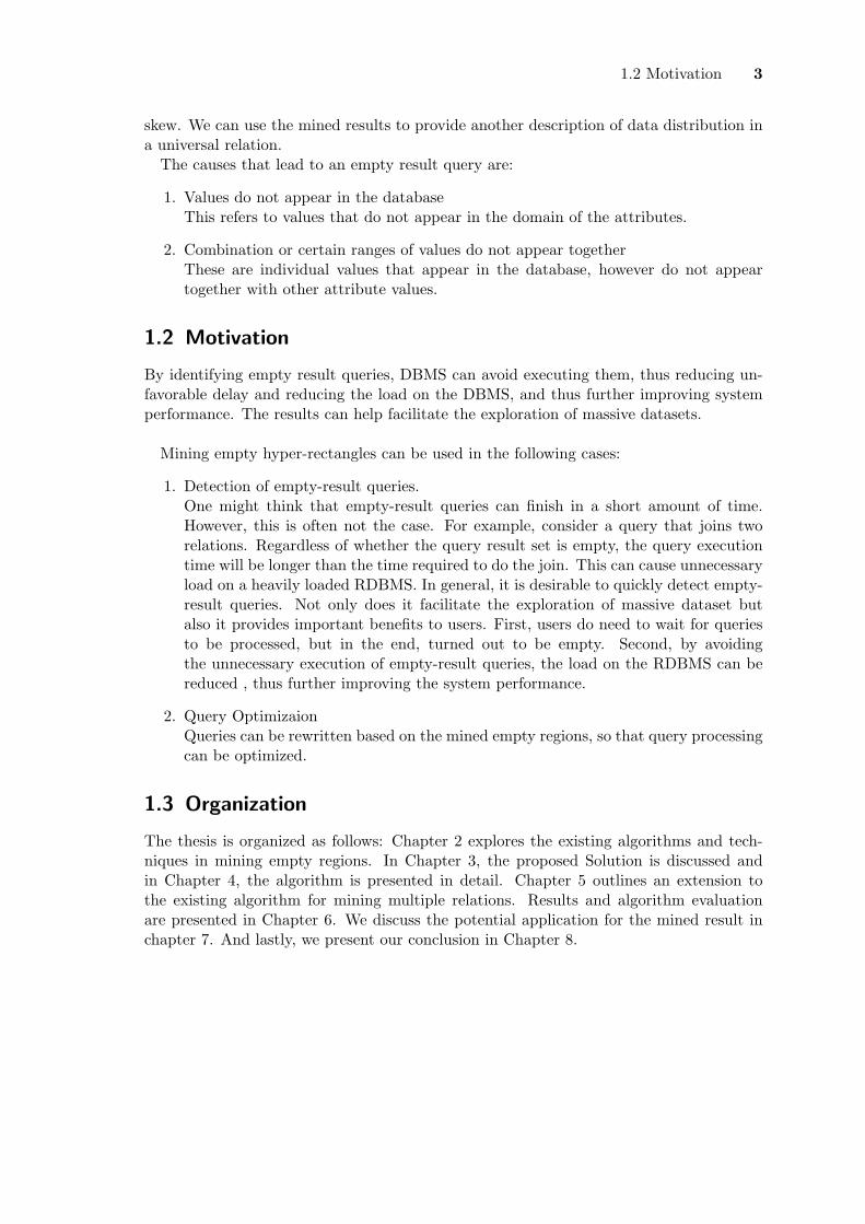
The causes that lead to an empty result query are:
1. Values do not appear in the databaseThis refers to values that do not appear in the domain of the attributes.
2. Combination or certain ranges of values do not appear togetherThese are individual values that appear in the database, however do not appeartogether with other attribute values.
1.2 Motivation
By identifying empty result queries, DBMS can avoid executing them, thus reducing un-favorable delay and reducing the load on the DBMS, and thus further improving systemperformance. The results can help facilitate the exploration of massive datasets.
Mining empty hyper-rectangles can be used in the following cases:
1. Detection of empty-result queries.One might think that empty-result queries can finish in a short amount of time.However, this is often not the case. For example, consider a query that joins tworelations. Regardless of whether the query result set is empty, the query executiontime will be longer than the time required to do the join. This can cause unnecessaryload on a heavily loaded RDBMS. In general, it is desirable to quickly detect empty-result queries. Not only does it facilitate the exploration of massive dataset butalso it provides important benefits to users. First, users do need to wait for queriesto be processed, but in the end, turned out to be empty. Second, by avoidingthe unnecessary execution of empty-result queries, the load on the RDBMS can bereduced , thus further improving the system performance.
2. Query OptimizaionQueries can be rewritten based on the mined empty regions, so that query processingcan be optimized.
1.3 Organization
The thesis is organized as follows: Chapter 2 explores the existing algorithms and tech-niques in mining empty regions. In Chapter 3, the proposed Solution is discussed andin Chapter 4, the algorithm is presented in detail. Chapter 5 outlines an extension tothe existing algorithm for mining multiple relations. Results and algorithm evaluationare presented in Chapter 6. We discuss the potential application for the mined result inchapter 7. And lastly, we present our conclusion in Chapter 8.

2Related Work
2.1 Different definitions used
In previous research literature, many different definitions of empty regions have been used.It is known as holes in [Liu et al., 1997] and Maximal empty Hyper-rectangle(MHR) in[Edmonds et al., 2001]. However, in [Liu et al., 1998], the definition of a hole is relaxed,where regions with low density is considered ’empty’. In this context, our definition ofa hole or empty hyper-rectangle is simply a region in the space that contains no datapoint. They exist because certain value combinations are not possible. In a continuousspace, there always exist a large number of holes because it is not possible to fill up thecontinuous space with data points.
In [Liu et al., 1997], they argued that not all holes are interesting, as they wish todiscover only holes that assist them in decision making or discovery of interesting datacorrelation. However in our case, we aim to mine holes to assist in query processing,regardless of their ’interestingness’.
2.2 Existing Techniques for discovering empty result queries
2.2.1 Incremental Solution
In [Luo, 2006], Luo proposed an incremental solution for detecting empty-result queries.The key idea is to remember and reuse the results from previously executed empty-resultqueries. Whenever empty-result queries are encountered, the query is analysed and thelowest-level of empty result query parts are stored in Caqp, known as the collection ofatomic query parts. It claims that the coverage detection capability in this method ismore powerful than that of the traditional materialized view method. Consequently, withstored atomic query parts, it can handle empty result queries based on two followingscenarios:
1. a more specific queryIt is able to identify using the stored atomic query part, queries that are morespecific. In this case, the query will not be evaluated at all.
2. a more general queryHowever, if a more general query is encountered, the query will be executed to
4

2.2 Existing Techniques for discovering empty result queries 5
determine whether it returns empty. If it does, the new atomic query parts that aremore general will replace the old ones.
Below are the main steps of breaking a lowest-level query part P whose output is emptyinto one or more atomic query parts:
1. Step 1: P is transformed into a simplified query part Ps.
2. Step 2: Ps is broken into one or more atomic query parts.
3. Step 3: The atomic query parts are stored in Caqp.
This method is not specific to any data types, as the atomic queries parts are directlyextracted from queries issued by users. Queries considered here can contain point-basedcomparisons and unbounded-interval-based comparison.
• point-based comparisons: (A.c =′ x′)
• unbounded-interval-based comparisons: (10 < A.a < 100, B.e < 40)
Unlike other data mining approaches, this method is built into a RDBMS and is imple-mented at the query execution level. First, the query execution plan is generated and thelowest-level query part whose output is empty is identified. These parts are then storedin Caqp and kept in memory for efficient checking.
One of main disadvantage of this solution is that it may need to take a long time toobtain a good set of Caqp, due to its incremental nature. Many empty result queries needto be executed first before the RDBMS can have a good detection of empty result queries.
2.2.2 Data Mining Solutions
Mining empty regions or holes is seen to be the complementary approach to existing datamining techniques that focuses on the discovery of dense regions, interesting groupings ofdata and similiarity between values. There mining methods however can be applied todiscover empty regions in the data. There have been studies on mining of such regions, andthey can be categorized into the following groups, described individually in each subsectionbelow.
Discovering Holes by Geometry
There are two algorithms that discover holes by using geometrical structure.
(1) Constructing empty rectangles
The algorithm proposed in [Edmonds et al., 2001] aims at constructing or ’growing’ emptycells and output all maximal rectangles. This method requires a single scan of a sorteddata set. This method works well in two dimension space, and can be generalized to highdimensions, however it might be complicated. The dataset is depicted as an |X| × |Y |matrix of 0’s and 1’s. 1 represents the presence of a value and 0 for non-existence of avalue, as shown in Figure 2.2(a). First it is assumed that the set X of distinct values (thesmaller) in the dimension is small enough to be stored in memory.
2.2 Existing Techniques for discovering empty result queries 6
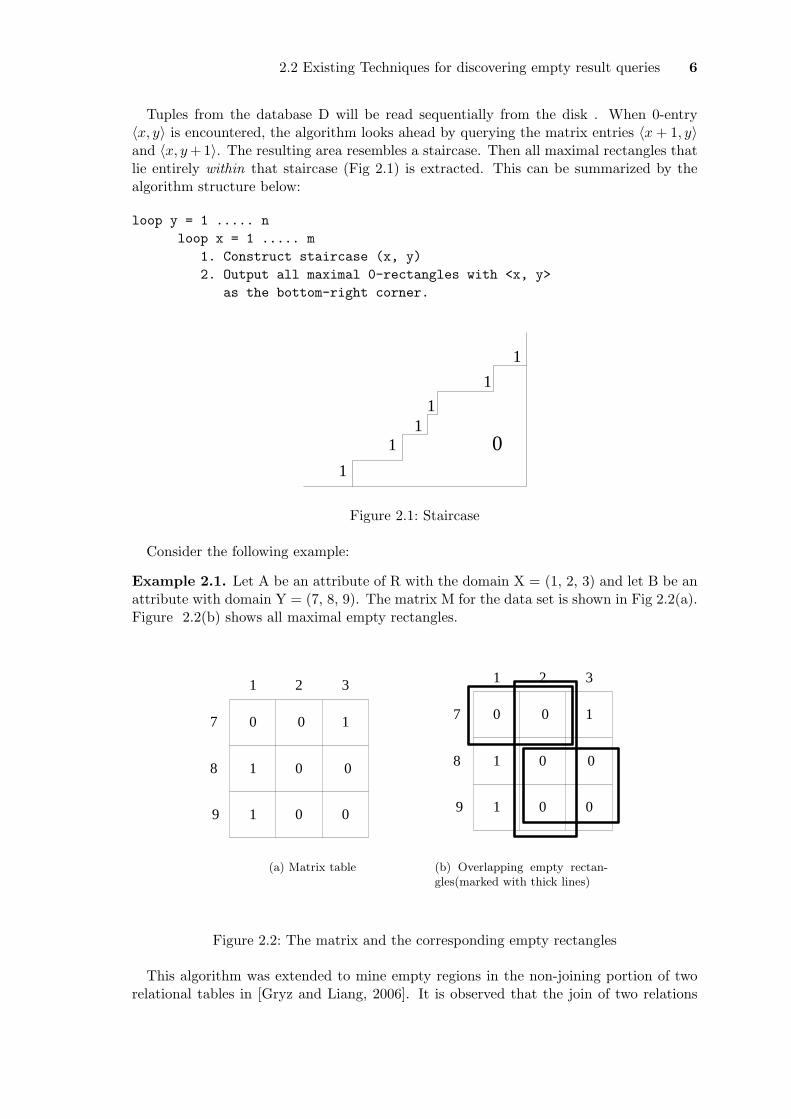
Tuples from the database D will be read sequentially from the disk . When 0-entry〈x, y〉 is encountered, the algorithm looks ahead by querying the matrix entries 〈x + 1, y〉and 〈x, y + 1〉. The resulting area resembles a staircase. Then all maximal rectangles thatlie entirely within that staircase (Fig 2.1) is extracted. This can be summarized by thealgorithm structure below:
loop y = 1 ..... nloop x = 1 ..... m
1. Construct staircase (x, y)2. Output all maximal 0-rectangles with <x, y>
as the bottom-right corner.
01
11
1
1
1
Figure 2.1: Staircase
Consider the following example:
Example 2.1. Let A be an attribute of R with the domain X = (1, 2, 3) and let B be anattribute with domain Y = (7, 8, 9). The matrix M for the data set is shown in Fig 2.2(a).Figure 2.2(b) shows all maximal empty rectangles.
0 0
0 0
0 0
1
1
1
1 2 3
7
8
9
(a) Matrix table
0 0
0 0
0 0
1
1
1
1 2 3
7
8
9
(b) Overlapping empty rectan-gles(marked with thick lines)
Figure 2.2: The matrix and the corresponding empty rectangles
This algorithm was extended to mine empty regions in the non-joining portion of tworelational tables in [Gryz and Liang, 2006]. It is observed that the join of two relations

2.2 Existing Techniques for discovering empty result queries 7
in real databases are usually much smaller than their Cartesian product. The ranges andvalues that do not appear together are characterized as empty regions. It is observedthat this method generates a lot of overlapping rectangles, as shown in Figure 2.2(b).Even though it is shown that the number of overlapping rectangles is at most O(|X| |Y |),there are still a lot of redundant results and the number of empty rectangles might notaccurately show the empty regions in the data.
The number of maximal hyper-rectangles in a d-dimensional matrix is O(n2d−2) wheren = |X| × |Y |. The complexity of an algorithm to produce them increases exponentiallywith d. When d = 2 dimensions, the number of maximal hyper-rectangles is O(n2), whichis linear in the size O(n2) of the input matrix. As for d = 3 dimensions, the numberincreases to O(n4), which is not likely to be practical for large datasets.
(2)Splitting hyper-rectangles.
The second method introduced in [Liu et al., 1997] Maximal Hyper-rectangle(MHR) isformed by splitting existing MHR when a data point is added.
Given k-dimensional continuous space S, and n points in S, they first start with oneMHR, which occupies the entire space S. Then each point is incrementally added toS. When a new point is added, they identify all the existing MHRs that contain thatpoint. Using the newly added point as reference, a new lower and upper bound for eachdimension is formed to result in 2 new hyper-rectangles along that dimension. If the newhyper-rectangles are found to be sufficiently large, they are inserted into the list of MHRsto be considered. At each insertion, they update the set of MHRs.
1
2A K E B
G
Q
CFMD
max2
max1min1
min2
Figure 2.3: Splitting of the rectangles
As shown in Figure 2.3, the new rectangles formed after points P1 and P2 are inserted.The rectangles are split along dimension 1 and dimension 2, resulting in new smallerrectangles. Only sufficiently large ones are kept. The proposed algorithm is memory-based and is not optimized for large datasets. As the data is scanned, a data structure iskept storing all maximal hyper-rectangles. The algorithm runs in O(|D|2(d−1) d3(log |D|)2)where d is the number of dimensions in the dataset. Even in two dimensions (d = 2), thisalgorithm is impractical for large datasets. In an attempt to address both the time andspace complexity, the authors proposed to maintain only maximal empty hyper-rectanglesthat exceed an a user defined minimum size.
The disadvantage of this method is that it is impractical for large dataset. Besides that,results might not be desirable if the dataset is dense. In this case, a lot of small empty

2.2 Existing Techniques for discovering empty result queries 8
regions will be mined. This solution only works for continuous attributes and it does nothandle discrete attributes.
Discovering Holes by Decision Trees Classifiers
In [Liu et al., 1998], Liu et. alproposed to use decision tree classifiers to (approximately)separate occupied from unoccupied space. They then post-process the discovered regionsto determine maximal empty rectangles. It relaxes the definition of a hole, to that of aregion with count or density below a certain threshold is considered a hole. However, theydo not guarantee that all maximal empty rectangles are found. Their approach transformsthe holes-discovery problem into a supervised learning task, and then uses the decisiontree induction technique for discovering holes in data. Since decision trees can handle bothnumeric and categorical values, this method is able to discover empty regions in mixeddimensions. This is an advantage over the other methods as they are not only able tomine empty rectangles in numeric dimensions, but also in mixed dimensions of continuousand discrete attributes.
This method is built upon the method in [Liu et al., 1997] (discussed above underDiscovering Holes by Geometry - Splitting hyper-rectangles). Instead of using points asinput to split the hyper-rectangle space, this method uses filled regions, FR as input toproduce maximal holes.
This method consists of the following three steps:
1. Partitioning the space into cells.Each continuous attribute is first partitioned into a number of equal-length intervals(or units). Values have to be carefully chosen to ensure that the space is partitionedinto suitable cell size.
2. Classifying the empty and filled regions.A modified version of decision tree engine in C4.5 is used to carve the space intofilled and empty regions. With the existing points, the number of empty cells arecalculated by minusing the filled cells from the total number of cells. With thisinformation, C4.5 will be able to compute the information gain ratio and use it todecide the best split. A decision tree is constructed, with tree leafs labeled empty,representing empty regions, and the others the filled region, FR.
3. Producing all the maximal holes.In this post-processing step, all the maximal holes are produced. Given a k-dimensionalcontinuous space S and n FRs in S, they first start with one MHR which occupiesthe entire space S. Then each FD is incrementally added to S. At each insertion, theset of MRHs found is updated. When a new FR is added, they identify all the exist-ing NHRs that intersect with this FR. These hyper-rectangles are no longer MHRssince they now contain part of the FR within their interior. They are then removedfrom the set of existing MHRs. Using the newly added FR as reference, a new lowerand upper bound for each dimension are formed to result in 2 new hyper-rectanglesalong that dimension. If these new hyper-rectangles are found to be MHRs and aresufficiently large, they are inserted into the list of existing MHRs, otherwise they arediscarded.
As shown in Figure 2.4, the new rectangles are formed after FRs H1 and H2 are inserted.The hyper-rectangles are split, forming smaller MHRs. Only sufficiently large ones are

2.2 Existing Techniques for discovering empty result queries 9
kept. The final set of MHRs are GQNH, RBCS, GBUT, IMND, OPCD, AEFD and ABLKrespectively.
1
2
A
K
E BG Q
CF
M
D
max2
max1min1
min2
R
L
UJ
P
H N S
T
O
I
H1
H2
Figure 2.4: Carving out the empty rectangles using decision tree
2.2.3 Analysis
It is true that mining empty regions is not an easy task. As some of the mining methodsproduce a large number of empty rectangles. To counter this problem, a user input isrequired and mining is done only on regions with size larger than the user’s specification.Another difficulty is the inability of existing methods to mine discrete attributes or thecombination of continuous and discrete values. Most of the algorithms scale well only inlow-dimensional space, eg: 2 or 3 dimension. They immediately become impractical ifmining is needed to be done high dimensional space.
It is stated that not all holes are important in [Liu et al., 1997], however our task isto store as many large discovered empty hyper-rectangles. It is noticed that there are noclustering techniques used. Simple observation is that existing clustering methods findhigh density data and ignore low density regions. Existing clustering techniques such asCLIQUE [Agrawal et al., 1998] find clusters in subspaces of high dimensional data, butonly works for continuous values and only works for high density data and ignore lowdensity ones. In this, we want to explore the usage of clustering in finding empty regionsof the data.

3Proposed Solution
3.1 General Overview
In view of the goal of mining for empty result queries, we propose to mine empty regionsin the dataset to achieve that purpose. Empty result queries happens when the requiredregion turns out to be empty, containing no points. Henceforth, we will focus on miningempty region, which is seen as equivalent to mining empty result queries. More specifically,empty regions here mean empty hyper-rectangles. We concentrate on hyper-rectangularregions instead of finding irregular regions described by some of the earlier mining methods,like the staircase-like region [Edmonds et al., 2001] or irregular shaped regions due tooverlapping rectangles.
VQ
x1
xj
x0
xi
y1y0 yi yj
Figure 3.1: Query and empty region
SELECT * FROM tableWHERE X BETWEEN x_i AND x_jAND Y BETWEEN y_i AND y_j;
To illustrate the relation between empty result queries and empty regions in databaseviews, consider Figure 3.1 and the SQL query above. The shaded region V is a materializedview depicting an empty region in the dataset and the rectangle box Q with thick linesdepicts the query. It is clear the given SQL query is an empty result query since the queryfalls within the empty region of the view.
10

3.2 Terms and definition 11
To mine these empty regions, the proposed solution uses the clustering method. In anutshell, all existing points are clustered into clusters, and empty spaces are inferred fromthem. For this method, no prior domain knowledge is required. With the clustered data,we use the itemset lattice and a levelwise search to permutate and mine for empty regions.
Here are the characteristics of the proposed solution:
• works for both categorical and continuous values.
• allows user can choose the granularity of the mined rules based on their requirementand the available memory.
• characterize regions strictly as rectangles, unlike in [Gryz and Liang, 2006], whichhas overlapping rectangles and odd-shaped regions.
• implements independently on the size of the dataset, just dependent on the Cartesianproduct of the size of each attribute domain.
• operates with the running time that is linear in the size of the attributes.
3.2 Terms and definition
Throughout the whole thesis, the following terms and definitions are used.
Database and attributes:
Let D be a database of N tuples, and let A be the set of attributes, A = {A1, ...An},with n distinct attributes. Some attributes take continuous values, and other attributestake discrete values. For a continuous attribute Ai, we use mini and maxi to denote thebounding (minimum and maximum) values. For a discrete attribute Ai, we use dom(Ai)to denote its domain.
Empty result queries
Empty result queries are queries that are processed by a DBMS and returns 0 tuples.The basic assumption is that all relations are non-empty. All tuples in the dataset arecomplete and contains no missing values. From this, we can assert that all plain projectionqueries are not empty. Therefore we only consider selection-projection queries, which maypotentially evaluates to empty.
1. Projection queries:q = πX(R) is not empty if relation R is not empty.
2. Selection-projection queries with one selection:q = πX(σAi=ai(R)) is not empty since Ai ∈ A and ai ∈ dom(Ai).
It is noted that the more specific the query (i.e: a query that has more selection clauses),the more chances that it might evaluate to empty. By using a levelwise method, thissolution mines such selection combinations from each possible combination of attributes.In the domain of our testing, we only consider values that are in the domain, as for numericvalues, the domain is the set of clusters formed by the continuous values.

3.2 Terms and definition 12
Query selection criteria
Query selection criteria can have the following format:
• for discrete attributes: {(Ai = ai)|(Ai ∈ A) and ai ∈ dom(Ai))}
• for continuous attributes: {Aj op x|x, y ∈ R, op ∈ {=, <,>,≤,≥}}
Minimal empty selection criteria
We are interested in mining only the minimal empty selection criteria that makes a queryempty. We have established that empty result may only appear in selection-projectionqueries. Therefore we focus our attention to the selection criteria of a query. The propertyof being empty is monotonic, in which if a set of selection criteria causes a query to beempty, then any superset of it will also be empty.
Definition 3.1. Monotone. Given a set M , E denotes the property of being empty, andE is defined over the powerset of M is monotone if
∀S, J : (S ⊆ J ⊆ M ∧ E(S)) ⇒ E(J).
Monotonicity of empty queries:Let q = πX(σs(R)) where X ⊆ A. The selection criteria s = {Ai = ai, Aj = aj} wherei 6= j, Ai 6= Aj and Ai, Aj ∈ A. If we know that ans(q) = ∅, then any selection s′, wheres ⊆ s′, will produce an empty result too.
Hence, our task is to mine only minimal selection criteria that makes a query empty.
Hyper-rectangle
Based on the above database and query selection criteria definitions, we further define thesyntax of empty hyper-rectangles, EHR:
1. (Aij = vij ) with vij ∈ aij if Aij is a discrete attribute, or
2. (Aij , lij , uij ) with minij ≤ lij ≤ maxij if Aij is a continuous attribute.
EHRs have the following properties:
1. Rectilinear: All sides of EHR are parallel to the respective axis, and orthogonal tothe others.
2. Empty: EHR does not have any points in its interior.
Multidimensional space and subspace:
We have that A = {A1, A2, . . . , An}, let S = A1 ×A2 × ....×An be a n-dimensional spacewhere each dimension Ai is of two possible types: discrete and continuous. Any spacewhose dimensions are a subset of A1, A2, ..., An is known as the subspace of S. we willrefer to A1, . . . , An as the dimensions of S.
3.2.1 Semantics of an empty region
This solution works on heterogeneous attributes, and here we focuses on two commontypes of attributes, namely discrete and continuous valued attributes. With this, we havethree different combinations of attribute types, forming three different types of subspaces.Below we give the semantic definitions of an empty region of each such subspaces:

3.3 Method 13
Discrete attributes:
We search for the combination of attribute-value pairs that does not exist in the database.Consider the following illustration:A1: dom(A1) = {a11 , a12 , ...., a1m}, where |A1| = m.A2: dom(A2) = {a21 , a22 , ...., a2n}, where |A2| = n.Selection criteria, σ: A1 = ai ∧ A2 = bj
where a1i ∈ dom(A1) and a2j ∈ dom(A2), but this combination, A1 = ai ∧ A2 = bj doesnot exist in any tuple in the database.
Continuous attributes:
An empty hyper-rectangle is a subspace that consist of only connected empty cells. Givena k-dimensional continuous space S bounded in each dimension i (1 ≤ i ≤ k) by a mini-mum and a maximum value (denoted by mini and maxi), a hyper-rectangle in S is definedas the region that is bounded on each dimension i by a minimum and a maximum bound.A hyper-rectangle has 2k bounding surfaces, 2 on each dimension. The two boundingsurfaces on dimension i are parallel to axis i and orthogonal to all others.
Mixture of continuous and discrete attributes:
Without loss of generality, we assume that the first k attributes are discrete attributes,A1, ...Ak, and the rest are continuous attributes, Ak+1, ....Am. A cell description is asfollows:
(discrete− cell, continuous− cell)
which discrete− cell is a cell in the discrete subspace, which is ((A1 = a1), .....) with ai
∈ dom(Ai), and continuous− cell is a cell in the continuous subspace for Ak+1, ...Am. Anhyper-rectangle is represented with
(discrete− region, continuous− region)
It is a region consisting of a set of empty cells, where discrete− region is a combinationof attribute-value pairs and continuous − region is a set of connected empty cells in thecontinuous subspace.
In theory, an empty region can be of any shape. However, we focus only on hyper-rectangle regions instead of irregular regions as described by a long disjunction of con-junctions (Disjunctive Normal Form used in [Agrawal et al., 1998]), or as x-monotoneregions described in [Fukuda et al., 1996].
3.3 Method
3.3.1 Duality concept
We present here the duality concept of the itemset lattice in a levelwise search. Considerthe lattice illustrated in Figure 3.2, (with the set of attributes A = {A, B, C, D}). Atypical frequent itemset algorithm looks at one level of the lattice at a time, starting fromthe empty itemset at the top. In this example, we discover that the itemset {D} is not1-frequent (it is empty). Therefore, when we move on to successive levels of lattice, we do

3.3 Method 14
Figure 3.2: The lattice that forms the search space
not have to look at any supersets of {D}. Since half of the lattice is composed of supersetsof {D}, this is a dramatic reduction of the search space.
Figure 3.2 illustrates this duality. Supposed we want to find the combinations that areempty. We can again use the level-wise algorithm, this time starting from the maximalcombination set = {A, B, C, D} at the bottom. As we move up levels in the lattice byremoving elements from the combination set, we can eliminate all subset of a non-emptycombination. For example, the itemset {A, B, C} is empty, so we can remove half of thealgebra from our search space just by inspecting this one node.
There are two trivial observations here:
1. Apriori can be applied to any constraint P that is antimonotone. We start from theempty set and prune supersets of sets that do not satisfy P.
2. Since itemset lattice can be seen as a boolean algebra, so Apriori also applies to amonotone Q. We start from the set of all items instead of the empty set. Then prunesubsets of sets that do not satisfy Q.
The concept of duality is useful in this context, as the proposed solution is formulatedbased on it. Further discussion of the usage of this duality is found in the next chapter,where the implementation of the solution is also discussed in detail.
4Algorithm
From the duality concept defined earlier, we could tackle the problem of mining emptyhyper-rectangles, known as EHR using either the positive pruning or the negative pruningapproach. This is further elaborated in the following:
1. Monotonicy of empty itemsetWe have seen that the property of being empty is monotonic, and we could makeuse of negative pruning in the lattice. If k-combination is empty, then all k + 1-combination is also empty. Starting from the largest combination, any combinationproven not to produce an empty query, is pruned off from the lattice, and subse-quently all of its subset are not considered. This is known as negative pruning.
2. Anti-monotonicity of 1-frequent itemsetInterestingly, this property can be characterized in the form of its duality. A k-combination is empty also means that that particular combination does not have afrequency of at least 1. Therefore, this problem can bee seen as mining all 1-frequentcombination. This in turn is anti-monotonic. If k-combination is not 1-frequent, thenall k + 1-combination cannot be 1-frequent. In this case, we can use the positivepruning in the lattice. Candidate itemset that are pruned away are the emptycombinations that we are interested in.
A selection criteria will be used to determine which method would evaluate best forthe given circumstances. This will be discussed in Section 4.3. In this chapter, we focusmainly on mining for EHR, empty regions bounded by continuous values. As we shall seethat the same method can be generalized and be applied to mine empty heterogeneousitemsets. All mined results are presented in the form of rules.
4.1 Preliminaries
4.1.1 Input Parameters
We require user to input parameters for this algorithm, however input parameters arelimited to the minimum, because the more input parameters we have, the harder it is toprovide the right combination for an optimum performance of the algorithm. User caninput the coverage parameter, τ . This will determine how fine grain the empty rectangleswill be. The possible values of τ ranges between 0 and 1. The detail usage of this parameteris discussed in Section 4.4.3.
15

4.1 Preliminaries 16
4.1.2 Attribute Selection
As mentioned earlier, mining empty result queries are restricted only on attributes thatare frequently referenced together in the queries. They can also be set of attributesselected and specified by the user. Statistical techniques for identifying the most influentialattributes for a given dataset, such as factor analysis and principal component analysisstated in [Lent et al., 1997] could also be used. In this algorithm, we consider both discreteand continuous attributes.
1. Discrete Attributes:Only discrete attributes with low cardinality are considered. As it makes no sense tomine attributes with large domains like ’address’ and ’names’. We limit the maximalcardinality of each domain to be 10.
2. Continuous Attributes:Continuous values are unrestricted, they can have an unbounded range. They willbe clustered and we limit the maximum number of clusters or bins to be 100.
4.1.3 Maximal set, max set
The maximal set is the Cartesian product of the values in the domain of each attribute. Itmakes up the largest possible search space for the algorithm. It represents all the possiblepermutations of the values. The maximal attribute set, max set .
max set = {dom(A1) × dom(A2) × . . .× dom(An)} (4.1)
and the size of max set is:
|max set| = |dom(A1)| × |dom(A2)| × . . . |dom(An)| (4.2)
4.1.4 Example
Consider Table 4.1, it contains the the flight information. This toy example will be usedthroughout this chapter.
FlightFlight No airline destination priceF01 SkyEurope Athens 0.99F02 SkyEurope Athens 1.99F03 SkyEurope Athens 0.99F04 SkyEurope Vienna 49.99F05 SkyEurope London 299.99F06 SkyEurope London 48.99F07 SkyEurope London 49.99F08 EasyJet Dublin 299.99F09 EasyJet Dublin 300.00F10 EasyJet Dublin 300.99
Table 4.1: Flight information table
4.2 Step 1: Data Preprocessing 17
Main Algorithm:
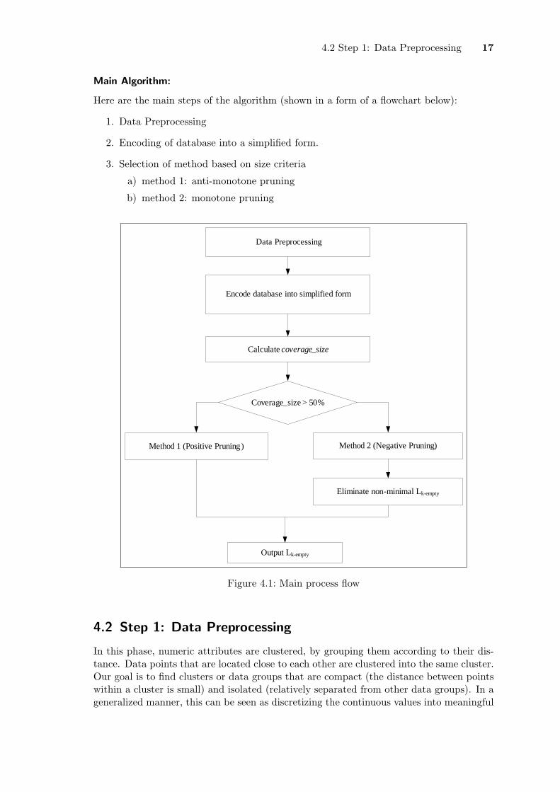
Here are the main steps of the algorithm (shown in a form of a flowchart below):
1. Data Preprocessing
2. Encoding of database into a simplified form.
3. Selection of method based on size criteria
a) method 1: anti-monotone pruning
b) method 2: monotone pruning
Data Preprocessing
Encode database into simplified form
Calculate coverage_size
Coverage_size > 50%
Method 1 (Positive Pruning) Method 2 (Negative Pruning)
Eliminate non-minimal Lk-empty
Output Lk-empty
Figure 4.1: Main process flow
4.2 Step 1: Data Preprocessing
In this phase, numeric attributes are clustered, by grouping them according to their dis-tance. Data points that are located close to each other are clustered into the same cluster.Our goal is to find clusters or data groups that are compact (the distance between pointswithin a cluster is small) and isolated (relatively separated from other data groups). In ageneralized manner, this can be seen as discretizing the continuous values into meaningful

4.2 Step 1: Data Preprocessing 18
ranges based on the data distribution. Existing methods include equi-depth, equi-widthand distance-based that partitions continuous values into intervals. However, both equi-depth and equi-width are found not to be able to capture the actual data distribution, thusare not suitable to be used in the discovery of empty regions. Here, an approach that issimilar to distance-based partitioning as described in [Miller and Yang, 1997] is used.
Existing clustering strategies aims at finding densely populated region in a multi-dimensional dataset. Here we only consider finding clusters in one dimension. As explainedin [Srikant and Agrawal, 1996], one dimensional cluster is the range of smallest intervalcontaining all closely located points. We employ an agglomerative hierarchical cluster-ing method to cluster points in one dimension. An agglomerative, hierarchical clusteringstarts by placing each object in its own cluster and then merges these atomic clusters intolarger and larger clusters until all objects are in a single cluster.
The purpose of using hierarchical clustering is to identify groups of clustered pointswithout recourse to the individual objects. In our case, it is desirable to identify aslarge clustered size as possible because these maximal clusters are able to assist in findinglarger region of empty hyper-rectangles. We shall see the implementation of this idea inthe coming sections.
Y
X
CX1
Y
CX2 CX3X
CY1
CY2
CY3
Figure 4.2: Clusters formed on X and Y respectively
Figure 4.2 shows a graph with points plotted with respect to two attributes, X and Y.These points are clustered into two sets of clusters, one in dimension X, and the other indimension Y. When the dataset is projected on the X-axis, 3 clusters are formed, namelyCX1, CX2 and CX3. Similarly, CY 1, CY 2 and CY 3 are 3 clusters formed when the datasetis projected on the Y-axis.
The clustering method used here is an modification to the BIRCH(Balanced IterativeReducing and Clustering using Hierarchies) clustering algorithm introduced by Zhang etal. in [Zhang et al., 1996]. It is an adaptive algorithm that has linear IO cost and is ableto handle large datasets.
The clustering technique used here shares some similarities with BIRCH. First theyboth uses the distance-based approach. Since data space is usually not uniformly occupied,hence, not every data point is equally important for the clustering purpose. A dense regionof points is treated collectively as a single cluster. In both techniques, clusters are organisedand characterized by the use of an in-memory, height-balance tree structure (similar to aB+-tree). This tree structure is known as CF-tree in BIRCH, while here it is referred asRange Tree. The fundamental idea here is that clusters can be incrementally identified

4.2 Step 1: Data Preprocessing 19
and refined in a single pass over the data. Therefore, the tree structure is dynamicallybuilt, and only requires a single scan of the dataset. Generally, these two approachesshare the same basic idea, but differs only in two minor portions: First, the CF Tree usesClustering Feature(CF) for storage of information while the Range tree stores informationin the leaf nodes. Second, CF tree is rebuilt when it runs out of memory, Range Tree onthe other hand is fixed with a maximum size, hence will not be rebuilt. The differencebetween this two approach will be highlighted in detail as each task of forming the tree isdescribed.
Storage of information
In BIRCH, each cluster is represented by a Clustering Feature (CF) that holds the sum-mary of the properties of the cluster. The clustering process is guided by a height-balancedtree of CF vectors. A Clustering Feature is s a triple summarizing the information abouta cluster. For Cx = {t1, . . . , tN}, the CF is defined as:
CF (Cx) = (N,N∑
i=1
ti[ ~X],N∑
i=1
ti[X]2)
where N is the number of points in the cluster, second being the linear sum of N datapoints, and third, the squared sum of the N data points. BIRCH is a clustering methodfor multidimensional and it uses the linear sum and square sum to calculate the distancebetween a point to the clusters. Based on the distance, a point is placed in the nearestcluster.
The Range-tree stores information in it’s leaf nodes instead of using Clustering Feature.Each leaf node represents a cluster, and they store summary of information of that cluster.Clusters are created incrementally and represented by a compact summary at every levelof the tree. Let the root of the hierarchy be at level 1, it’s children at level 2 and so on.A node in level i corresponds to the union of range formed by its children at level i + 1.For each leaf node in the Range tree, it has the following attributes:
LeafNode(min,max, N, sum)
• min: the minimum value in the cluster
• max: the maximum value in the cluster
• N : the number of points in the cluster
• sum:∑N
i=1 Xi
The centroid of a cluster is the mean of the points in the cluster. It is calculated asfollows:
centroid =∑N
i=1 Xi
N(4.3)
The distance between clusters can be calculated using the centroid Euclidean distance,Dist. It is calculated as follows:
Dist =√
(centroid1 − centroid2)2 (4.4)
Together, min and max defines the left and right boundaries of the cluster. The distanceof a point to a cluster is the distance of the point from the centroid of that cluster. A new

4.2 Step 1: Data Preprocessing 20
point is placed in the nearest cluster, i.e. the centroid with the smallest distance to thepoint.
From the leaf nodes, the summary of information can be derived and stored by theirrespective parent node (non-leaf node). So a non-leaf node represents a cluster made upof all the subcluster represented by its entry. Each non-leaf node can be seen as providinga summary of all the subcluster connected to it. The parent nodes, nodei in the Rangetree, contains the summary information of their children node, nodei+1:
Non− leafNode(mini,maxi, Ni, sumi)
where mini = MIN(mini+1), maxi = MAX(maxi+1), Ni =∑
Ni+1 and sumi =∑sumi+1
Range Tree
The Range-tree is built incrementally by inserting new data points individually. Eachdata point is inserted by locating the closest node. At each level, the closest node isupdated to reflect the insertion of the new point. At the lowest level, the point is addedto the closest leaf node. Each node in the Range-Tree is used to guide a new insertioninto the correct subcluster for clustering purposes, just the same as a B+-tree is used toguide a new insertion into the correct position for sorting purposes. The range tree is aheight-balanced tree with two parameters: branching factor B and size threshold T .
In BIRCH, the threshold T is initially set to 0 and the B is set based on the size ofthe page. As data values are inserted into the CF-tree, if a cluster’s diameter exceeds thethreshold, it is split. This split may increase the size of the tree. If the memory is full,a smaller tree is rebuilt by increasing the diameter threshold. The rebuilding is done byre-inserting leaf CF nodes into the tree. Hence, the data or the portion of the data thathas already been scanned does not need to be rescanned. With the higher threshold, someclusters are likely to be merged, reducing the space required by the tree.
In our case, the maximum size of the Range-tree is bounded, and therefore will not havethe problem of running out of memory. We have placed a limit on the size of the tree bypredefining the threshold T with the following calculation:
T =(maximum value−minimum value)
max cluster(4.5)
where maximum value and minimum value are the largest and the smallest value re-spectively for an attribute.
The maximum number of cluster, max cluster for each continuous value is set to be100. We have set the branching factor B = 4, where each nonleaf node contains at most4 children. A leaf node must satisfy a threshold requirement, in which the interval sizeof the cluster has to be less than the threshold T . The interval size of each clustering isthe range or interval bounded by between the min and the max.
interval size = max−min (4.6)
Insertion into a Range Tree
When a new point is inserted, it is added into the Range-tree as follows:
1. Identifying the appropriate leaf: Starting from the root, it recursively descends theRange-tree by choosing the closest node where the point is located within the minand max boundary of a node.

4.2 Step 1: Data Preprocessing 21
2. Modifying the leaf: When it reaches a leaf node, and if the new point falls within themin and max boundary, it is ’absorbed’ into the cluster, values of N and sum arethen updated. If a point does not fall within the min and max boundary of a leafnode, it first finds the closest leaf entry, say Li, and then test whether interval sizeof the augmented cluster satisfy the threshold condition. If so, the new point isinserted into Li. All values in Li: (min, max and N , sum) are updated accordingly.Otherwise, a new leaf node will be formed.
3. Splitting the leaf: If the number of branch reaches the limit of B, the branchingfactor, then we have to split the leaf node. Node splitting is done by choosing thefarthest pair of entries as seeds, and redistributing the remaining entries. Distancebetween the clusters are calculated using the centroid Euclidean distance, Dist inEquation 4.4. The levels in the Range tree will be balanced since it is a height-balanced tree, much in the way a B+-tree is adjusted in response to the insertion ofa new tuple.
In the Range-tree, the smallest clusters are stored in the leaf nodes, while non-leaf nodesstores the summary of the union of a few leaf nodes. The process of clustering can be seenas a form of discretizing the values into meaningful ranges.
In the last step of data preprocessing, the values in a continuous domain are replacedwith their respective clusters. The domain of the continuous attribute now consist of thesmallest clusters. Let Ai be an attribute with continuous values, and it is partitioned intom clusters, ci1, . . . cim. Now dom(Ai) = {ci1, ci2, . . . cim}.
Example 4.1. In the Flight Information example, the attribute price is a continuousattribute, with values ranging from 0.99 to 300.99.minimum value = 0.99, maximum value = 300.99, and we have set max cluster = 100.T is calculated as follows:
T =(300.99 − 0.99)
100= 3
Any points that falls within the distance threshold of T is absorbed into a cluster, whileall points with the interval size larger than T will form a cluster of its own. So all clustershave the maximum interval size of less than T . The values in price are clustered in thefollowing clusters:C1: [0.99, 1.99], C2: [48.99, 49.99], C3: [299.99, 300.99].Now the domain of price is defined in terms of these clusters, dom(price) = {[0.99, 1.99],[48.99, 49.99], [299.99, 300.99]}. The values in price are replaced with their correspondingclusters, as shown in Table 4.2.
Calculation of the size of the maximal set
After all the continuous attributes are clustered, now the domain of the continuous at-tributes are represented by the clusters. The cardinality of the domain is simply the num-ber of clusters. With these information, we are able to obtain the count of the maximal setdefined in Section 4.1. Recall that maximal set is obtained by doing the permutation ofvalues in the domain. From there, we can obtain the maximal set simply by permutatingthe values in the domain for each attributes. This information will be used in determiningwhich method to use, discussed in detail in Section 4.3.

4.3 Step 2: Encode database in a simplified form 22
FlightFlight No airline destination priceF01 SkyEurope Athens [0.99, 1.99]F02 SkyEurope Athens [0.99, 1.99]F03 SkyEurope Athens [0.99, 1.99]F04 SkyEurope Vienna [48.99, 49.99]F05 SkyEurope London [299.99, 300.99]F06 SkyEurope London [48.99, 49.99]F07 SkyEurope London [48.99, 49.99]F08 EasyJet Dublin [299.99, 300.99]F09 EasyJet Dublin [299.99, 300.99]F10 EasyJet Dublin [299.99, 300.99]
Table 4.2: Attribute price is labeled with their respective clusters
Example 4.2. Based on the Flight example, the size of the maximal set is calculated asfollows:dom(airline) = {SkyEurope, EasyJet}dom(destination) = {Athens, Vienna, London, Dublin}dom(age) = {[0.99, 1.99], [48.99, 49.99], [299.99, 300.99]}
|max set| = |dom(airline)| × |dom(destination)| × |dom(age)|= 24
4.3 Step 2: Encode database in a simplified form
In step 1, each continuous values are replaced with their corresponding cluster. Theoriginal dataset can then be encoded into a simplified form. The process of simplifying isto get a reduced representation of the original dataset, where only the distinct combinationof values are taken into consideration. Then we assign a tuple ID, known as the TID toeach distinct tuples. By doing this, we are reducing the size of the dataset, thus improvingthe runtime performance and the space requirement of the algorithm.
Since in essence, we are only interested in whether or not the combination exist, we donot need other information like the actual frequency of the occurence of those values. Itis the same like encoding the values in 1 and 0, with 1 to show that a value exist and0 otherwise. Unlike the usual data mining task, eg: finding densed region, clusters orfrequent itemset, in our case we do not need to know the actual frequency or density ofthe data. The main goal is to have a reduction in the size of the original database. Theresulting simplified database Ds will have only distinct values for each tuple.
ti = 〈a1i , a2i , . . . , ani〉
tj = 〈a1j , a2j , . . . , anj 〉
such that if i 6= j, then ti 6= tj , where i, j ∈ {1, . . . , n}.We sequentially assign a unique positive integer to Ds as an identifier for each tuple t.
Example 4.3. Consider the Table 4.2. It can be simplified into Table 4.3, Ds where itis the set of unique tuples with respect to the attributes airline, destination and price.These unique tuples are assigned an identifier, called TID.

4.3 Step 2: Encode database in a simplified form 23
FlightTID airline destination price1 SkyEurope Athens [0.99, 1.99]2 SkyEurope Vienna [48.99, 49.99]3 SkyEurope London [299.99, 300.99]4 SkyEurope London [48.99, 49.99]5 EasyJet Dublin [299.99, 300.99]
Table 4.3: The simplified version of the Flight information table
|Ds| = 5. In this example, Ds is 50% smaller than the original dataset.
Correctness
Ds is a smaller representation of the original dataset. Information is preserved in thisprocess of shrinking. Each point in a continuous attribute is grouped and representedby their respective clusters. Therefore Ds is just a coarser representation of the originaldataset, where the shape of the original data distribution is preserved. This simplificationdoes not change or affect the mining of EHR.
Distribution size
Next we calculate the percentage of the data distribution with the following equation:
distribution size =|Ds|
|max set|(4.7)
Example 4.4. In our example, we have |Ds| = 5, and |max set| = 24
distribution size =524
= 0.208
Trivial observation: only 21% of the value combination exist. The rest of them, with 79%are empty combinations, i.e: value combinations that does not exist in the dataset.
Method selection
distribution size is used to determine which of the two methods to use. If distribution size≤ 0.5, we will choose method 1. On the other hand method 2 will be chosen if distribution sizeis > 0.5. Observation on the value of distribution size are as follows:
• distribution size = 1: For this case, data distribution covers all the possible combi-nation of n-dimensions. In this situation, mining of EHR will not be done.
• 0 < distribution size ≤ 0.5: Data distribution covers less than half of the combina-tion. Data distribution is characterized as sparse.
• 0.5 < distribution size < 1: Data distribution covers more than half of the combi-nation. Data distribution is characterized as dense.
4.3 Step 2: Encode database in a simplified form 24
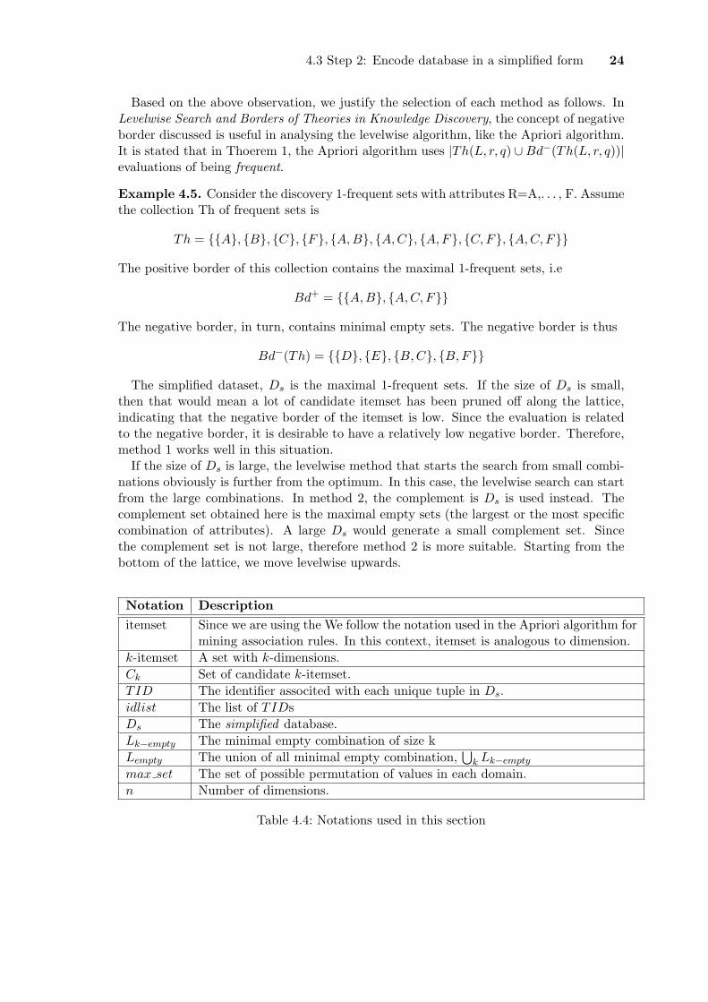
Based on the above observation, we justify the selection of each method as follows. InLevelwise Search and Borders of Theories in Knowledge Discovery, the concept of negativeborder discussed is useful in analysing the levelwise algorithm, like the Apriori algorithm.It is stated that in Thoerem 1, the Apriori algorithm uses |Th(L, r, q) ∪Bd−(Th(L, r, q))|evaluations of being frequent.
Example 4.5. Consider the discovery 1-frequent sets with attributes R=A,. . . , F. Assumethe collection Th of frequent sets is
Th = {{A}, {B}, {C}, {F}, {A,B}, {A,C}, {A,F}, {C,F}, {A,C, F}}
The positive border of this collection contains the maximal 1-frequent sets, i.e
Bd+ = {{A,B}, {A,C, F}}
The negative border, in turn, contains minimal empty sets. The negative border is thus
Bd−(Th) = {{D}, {E}, {B,C}, {B,F}}
The simplified dataset, Ds is the maximal 1-frequent sets. If the size of Ds is small,then that would mean a lot of candidate itemset has been pruned off along the lattice,indicating that the negative border of the itemset is low. Since the evaluation is relatedto the negative border, it is desirable to have a relatively low negative border. Therefore,method 1 works well in this situation.
If the size of Ds is large, the levelwise method that starts the search from small combi-nations obviously is further from the optimum. In this case, the levelwise search can startfrom the large combinations. In method 2, the complement is Ds is used instead. Thecomplement set obtained here is the maximal empty sets (the largest or the most specificcombination of attributes). A large Ds would generate a small complement set. Sincethe complement set is not large, therefore method 2 is more suitable. Starting from thebottom of the lattice, we move levelwise upwards.
Notation Description
itemset Since we are using the We follow the notation used in the Apriori algorithm formining association rules. In this context, itemset is analogous to dimension.
k-itemset A set with k-dimensions.Ck Set of candidate k-itemset.TID The identifier associted with each unique tuple in Ds.idlist The list of TIDsDs The simplified database.Lk−empty The minimal empty combination of size kLempty The union of all minimal empty combination,
⋃k Lk−empty
max set The set of possible permutation of values in each domain.n Number of dimensions.
Table 4.4: Notations used in this section
4.4 Step 3 - Method 1: 25
4.4 Step 3 - Method 1:
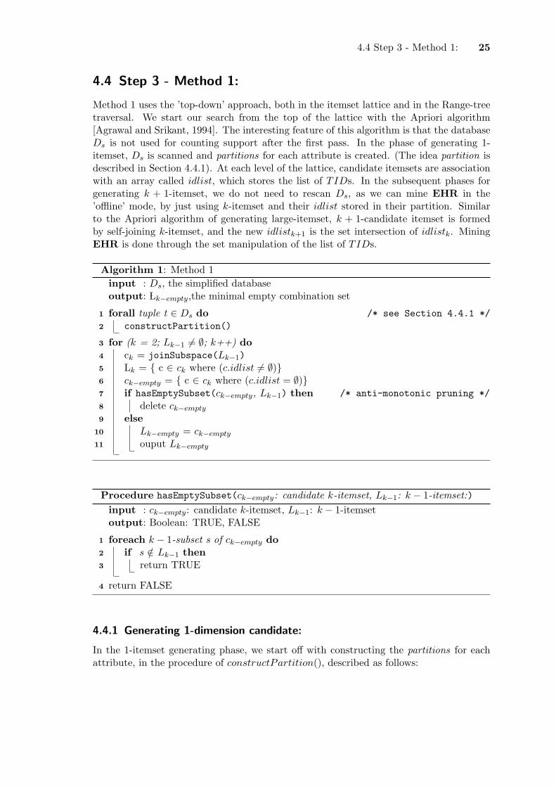
Method 1 uses the ’top-down’ approach, both in the itemset lattice and in the Range-treetraversal. We start our search from the top of the lattice with the Apriori algorithm[Agrawal and Srikant, 1994]. The interesting feature of this algorithm is that the databaseDs is not used for counting support after the first pass. In the phase of generating 1-itemset, Ds is scanned and partitions for each attribute is created. (The idea partition isdescribed in Section 4.4.1). At each level of the lattice, candidate itemsets are associationwith an array called idlist, which stores the list of TIDs. In the subsequent phases forgenerating k + 1-itemset, we do not need to rescan Ds, as we can mine EHR in the’offline’ mode, by just using k-itemset and their idlist stored in their partition. Similarto the Apriori algorithm of generating large-itemset, k + 1-candidate itemset is formedby self-joining k-itemset, and the new idlistk+1 is the set intersection of idlistk. MiningEHR is done through the set manipulation of the list of TIDs.
Algorithm 1: Method 1input : Ds, the simplified databaseoutput: Lk−empty,the minimal empty combination set
forall tuple t ∈ Ds do /* see Section 4.4.1 */1
constructPartition()2
for (k = 2; Lk−1 6= ∅; k++) do3
ck = joinSubspace(Lk−1)4
Lk = { c ∈ ck where (c.idlist 6= ∅)}5
ck−empty = { c ∈ ck where (c.idlist = ∅)}6
if hasEmptySubset(ck−empty, Lk−1) then /* anti-monotonic pruning */7
delete ck−empty8
else9
Lk−empty = ck−empty10
ouput Lk−empty11
Procedure hasEmptySubset(ck−empty: candidate k-itemset, Lk−1: k − 1-itemset:)input : ck−empty: candidate k-itemset, Lk−1: k − 1-itemsetoutput: Boolean: TRUE, FALSE
foreach k − 1-subset s of ck−empty do1
if s /∈ Lk−1 then2
return TRUE3
return FALSE4
4.4.1 Generating 1-dimension candidate:
In the 1-itemset generating phase, we start off with constructing the partitions for eachattribute, in the procedure of constructPartition(), described as follows:

4.4 Step 3 - Method 1: 26
Set partition
Each object in the domain is associated with their TID. The TID are stored in the formof set partition, a set of non-empty subsets of x such that every element xi ∈ X is exactlyone of the subset. The fundamental idea underlying our approach is to provide a reducedrepresentation of a relation. This can be achieved using the idea of partitions [Spyratos,1987, Huhtala et al., 1998]. Semantically, this has been explained in [Cosmadakis et al.,1986, Spyratos, 1987].
Definition 4.1. Partition. Two tuples ti and tj are equivalent with respect to a givenattribute set X if ti[A] = tj [A], for ∀ A ∈ X. the equivalance class of a tuple ti ∈ r withrespect to a given set X ⊆ R is defined by [ti]X = {tj ∈ r / ti[A] = tj [A], ∀ A ∈ X}. Theset πX = {[t]X / t ∈ r} of equivalance classes is a partition of r under X. That is, πX is acollection of disjoint sets of rows, such that each set has a unique value for the attributeset S, and the union of the sets equals the relation.
Example 4.6. Consider the simplified dataset in Table 4.3.Attribute airline has value ’SkyEurope’ in rows t1, t2, t3 and t4, so they form an equivalenceclass [t1]airline = [t2]airline = [t3]airline = [t4]airline = {1, 2, 3, 4}. The whole partition withrespect to attribute airline is πairline = {{1, 2, 3, 4}, {5}}. The table below summarizesthe partitions for L1, the 1-itemset.
Attribute Domain Partition
airline dom(airline) = {SkyEurope,EasyJet}
πairline = {{1, 2, 3, 4}, {5}}
destination dom(destination) = {Athens,Vienna, London, Dublin}
πdestination = {{1}, {2}, {3, 4}, {5}}
price dom(price) = {[0.99, 1.99],[48.99, 49.99], [299.99,300.99]}
range tree(price).child1 = {1},range tree(price).child2 = {2, 4},range tree(price).child3 = {3, 5}
Table 4.5: Partitions for L1
We store idlist with respect to the partitions in the following form:
• discrete values: set partitions are stored in a vector list called idlist.
• continuous values: set partitions are stored only in the leaf node of the Range-tree.The leaf nodes in a Range tree represents the smallest clusters. A nonleaf node, orknown as a parent node represents a cluster made up of all the subclusters of it’schildren node. The idlisti of a non-leaf node in level i are the union of all idlisti+1
of its child nodes are level i+1. To conserve space, idlist are only stored on the leafnodes. The idlist at a parent node are collected dynamically when needed by doingpost-order traversal on the Range-tree.
4.4.2 Generating k-dimension candidate
Subspace Clustering
First we start with low dimensionality, eliminating as many empty combinations as possiblebefore continuing with a higher dimension. The concept of candidate generation for each
4.4 Step 3 - Method 1: 27
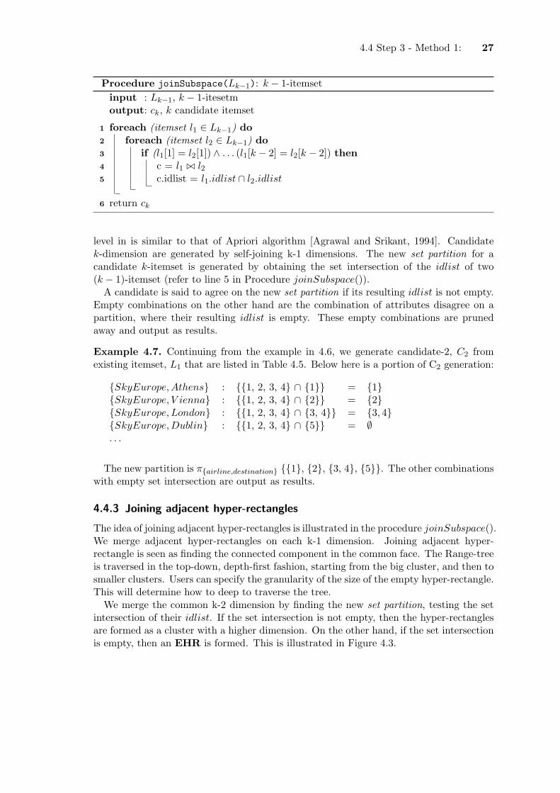
Procedure joinSubspace(Lk−1): k − 1-itemsetinput : Lk−1, k − 1-itesetmoutput: ck, k candidate itemset
foreach (itemset l1 ∈ Lk−1) do1
foreach (itemset l2 ∈ Lk−1) do2
if (l1[1] = l2[1]) ∧ . . . (l1[k − 2] = l2[k − 2]) then3
c = l1 ./ l24
c.idlist = l1.idlist ∩ l2.idlist5
return ck6
level in is similar to that of Apriori algorithm [Agrawal and Srikant, 1994]. Candidatek-dimension are generated by self-joining k-1 dimensions. The new set partition for acandidate k-itemset is generated by obtaining the set intersection of the idlist of two(k − 1)-itemset (refer to line 5 in Procedure joinSubspace()).
A candidate is said to agree on the new set partition if its resulting idlist is not empty.Empty combinations on the other hand are the combination of attributes disagree on apartition, where their resulting idlist is empty. These empty combinations are prunedaway and output as results.
Example 4.7. Continuing from the example in 4.6, we generate candidate-2, C2 fromexisting itemset, L1 that are listed in Table 4.5. Below here is a portion of C2 generation:
{SkyEurope,Athens} : {{1, 2, 3, 4} ∩ {1}} = {1}{SkyEurope, V ienna} : {{1, 2, 3, 4} ∩ {2}} = {2}{SkyEurope, London} : {{1, 2, 3, 4} ∩ {3, 4}} = {3, 4}{SkyEurope,Dublin} : {{1, 2, 3, 4} ∩ {5}} = ∅. . .
The new partition is π{airline,destination} {{1}, {2}, {3, 4}, {5}}. The other combinationswith empty set intersection are output as results.
4.4.3 Joining adjacent hyper-rectangles
The idea of joining adjacent hyper-rectangles is illustrated in the procedure joinSubspace().We merge adjacent hyper-rectangles on each k-1 dimension. Joining adjacent hyper-rectangle is seen as finding the connected component in the common face. The Range-treeis traversed in the top-down, depth-first fashion, starting from the big cluster, and then tosmaller clusters. Users can specify the granularity of the size of the empty hyper-rectangle.This will determine how to deep to traverse the tree.
We merge the common k-2 dimension by finding the new set partition, testing the setintersection of their idlist. If the set intersection is not empty, then the hyper-rectanglesare formed as a cluster with a higher dimension. On the other hand, if the set intersectionis empty, then an EHR is formed. This is illustrated in Figure 4.3.

4.4 Step 3 - Method 1: 28
(a) A filled rectanglein 2-dimension
(b) A filled rectangle in 2-dimension
(c) Joining at a connected component (d) Forming of an EHR
Figure 4.3: Joining adjacent hyper-rectangle
4.4 Step 3 - Method 1: 29
Joining of continous attributes:
In this case, Range-trees are compared in a top-down approach. The tree is travered depthfirst based on the user’s threshold input, τ . If the threshold is low, a bigger chunks of the ofempty region will be identified. Low threshold has better performance, however accuracywill be sacrificed. On the contrary, if the threshold is high, more empty hyper-rectanglewill be mined, but with finer granularity (i.e: size is smaller). More processing time willbe needed, as the tree needs to be traversed deeper.
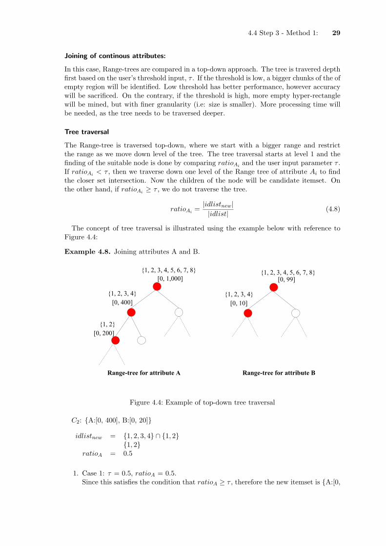
Tree traversal
The Range-tree is traversed top-down, where we start with a bigger range and restrictthe range as we move down level of the tree. The tree traversal starts at level 1 and thefinding of the suitable node is done by comparing ratioAi and the user input parameter τ .If ratioAi < τ , then we traverse down one level of the Range tree of attribute Ai to findthe closer set intersection. Now the children of the node will be candidate itemset. Onthe other hand, if ratioAi ≥ τ , we do not traverse the tree.
ratioAi =|idlistnew||idlist|
(4.8)
The concept of tree traversal is illustrated using the example below with reference toFigure 4.4:
Example 4.8. Joining attributes A and B.
Figure 4.4: Example of top-down tree traversal
C2: {A:[0, 400], B:[0, 20]}
idlistnew = {1, 2, 3, 4} ∩ {1, 2}{1, 2}
ratioA = 0.5
1. Case 1: τ = 0.5, ratioA = 0.5.Since this satisfies the condition that ratioA ≥ τ , therefore the new itemset is {A:[0,

4.4 Step 3 - Method 1: 30
400], B:[0, 20]}.
2. Case 2: τ = 0.75, ratioA = 0.5.ratioA < τ , therefore we need to traverse down the subtree of salary [0, 400]. Thenew candidate set is now {A:[0, 200], B:[0, 20]}.
idlistnew = {1, 2} ∩ {1, 2}{1, 2}
ratioA = 1.0
The condition of ratioA ≥ τ is satisfied, the new itemset is {A:[0, 200], B:[0, 20]}.
Mixture of discrete and continuous attributes:
The method discussed so far focused on mining EHR, however the method can be usedto mine heterogeneous types of attributes. In the case of combination of a continuous anda discrete attribute, instead of traversing two tree, here we are only traversing only onetree. We use a top-down approach to find the combination of empty results. The tree willbe traversed depth first based on user’s threshold input, τ . The higher the threshold, themore fine-grain the results. Each branch will traverse in a depth-first search manner untileither empty result is reached or count is above threshold. Here the EHR are representedas ’strips’.
For cases where it involves combination of only discrete attributes, the process of joiningthe attribute is straight forward, as it works just the same as itemset generation in Apriorialgorithm.
To mine for empty combinations, the same technique still applies. EHR or emptycombinations are candidates that have an empty set intersection in idlist.
4.4.4 Anti-monotonic Pruning
Anti-monotonic pruning, also known as positive pruning is used to reduce the numberof combinations we have to consider. Our aim is to mine 1-frequent combination whichhas the anti-monotonicity property. If k-combination is not 1-frequent, then all k + 1-combinations cannot be 1-frequent. Using this property, all superset of empty combina-tions will be pruned from the search space. Although pruned from the search space, theseare the results that we are interested in, so they are output and stored on disk as results.
The concept of anti-monotonic pruning is illustrated in Figure 4.5. A4 is found to beempty, and all supersets of A4 are pruned away from the search space.
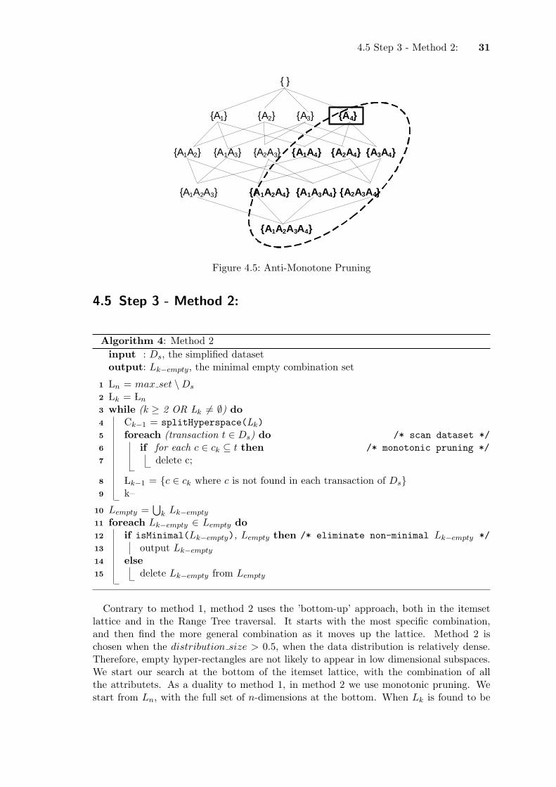
4.5 Step 3 - Method 2: 31
{ }
{A1} {A2} {A3} {A4}
{A1A2} {A1A3} {A1A4}{A2A3} {A2A4} {A3A4}
{A1A2A3} {A1A2A4} {A1A3A4} {A2A3A4}
{A1A2A3A4}
Figure 4.5: Anti-Monotone Pruning
4.5 Step 3 - Method 2:
Algorithm 4: Method 2input : Ds, the simplified datasetoutput: Lk−empty, the minimal empty combination set
Ln = max set \Ds1
Lk = Ln2
while (k ≥ 2 OR Lk 6= ∅) do3
Ck−1 = splitHyperspace(Lk)4
foreach (transaction t ∈ Ds) do /* scan dataset */5
if for each c ∈ ck ⊆ t then /* monotonic pruning */6
delete c;7
Lk−1 = {c ∈ ck where c is not found in each transaction of Ds}8
k–9
Lempty =⋃
k Lk−empty10
foreach Lk−empty ∈ Lempty do11
if isMinimal(Lk−empty), Lempty then /* eliminate non-minimal Lk−empty */12
output Lk−empty13
else14
delete Lk−empty from Lempty15
Contrary to method 1, method 2 uses the ’bottom-up’ approach, both in the itemsetlattice and in the Range Tree traversal. It starts with the most specific combination,and then find the more general combination as it moves up the lattice. Method 2 ischosen when the distribution size > 0.5, when the data distribution is relatively dense.Therefore, empty hyper-rectangles are not likely to appear in low dimensional subspaces.We start our search at the bottom of the itemset lattice, with the combination of allthe attributets. As a duality to method 1, in method 2 we use monotonic pruning. Westart from Ln, with the full set of n-dimensions at the bottom. When Lk is found to be

4.5 Step 3 - Method 2: 32
Procedure isMinimal(Lk−empty: k-empty itemset, Lempty: the full set of Lk−empty)
input : Lk−empty: k-empty itemset, Lempty: the full set of Lk−empty
output: Boolean: TRUE, FALSE
foreach k − 1-subset to 2-subset s of Lempty do1
if s /∈ Lempty then2
return TRUE3
return FALSE4
non-empty, we prune off this itemset. As we move levelwise upwards in the lattice, wegenerate candidate k − 1 from existing Lk. Instead of joining subspaces to form a higherdimension subspace, now we start with high dimension subspace and split the itemset toobtain candidates of lower subspaces.
4.5.1 Generating n-itemset
n-itemset is the biggest or the most specific combination that returns an empty result. InMethod 2, we start with n-itemset at the bottom level in the itemset lattice and work ourway up levelwise upwards. Recall that in step 2, the simplified database, Ds is obtained.Consequently, with the available information, n-itemset can be obtained by doing the setcomplement.
n− itemset = max set \Ds (4.9)
4.5.2 Generating k-1 itemset
Procedure splitHyperspace(k-itemset: Lk)
input : Lk, k-itemsetoutput: ck−1, k − 1-candidate itemset
foreach (itemset l ∈ Lk) do /* findCombination =(
kk−1
)*/1
csubset = findCombination(l, k-1)2
if for each c ∈ csubset /∈ ck−1 then /* keep unique candidate itemset */3
add c to ck−14
return ck−15
Splitting adjacent rectangles
This is the reverse of joining adjacent rectangles in method 1. At every level of the ofitemset lattice, the empty hyper-rectangles are split into smaller subspaces. Candidates ofsize k−1 is generated from k-itemset. At every level, the database will be scanned once tocheck whether the candidate itemsets are empty. If they are not, they will be pruned offfrom the search space. Candidate generation and dataset scan to evaluate the candidateitemset alternates until either the size of itemset reaches two, or no more candidates aregenerated.

4.5 Step 3 - Method 2: 33
Splitting of continuous attributes:
Tree traversal
Here we traverse the tree bottom up, starting with the smallest cluster at the leaf nodeand then generalize to a bigger one as we move up to the parent node. As we move up thelattice, we generate k − 1-itemset and ’generalize’ the ranges to a larger bounding range.At the bottom, we have the leaves of the tree, and as we generate the subset, we takevalues from the parents from the range tree. Since the Range-tree is a hierarchical tree, asmany as B (branching factor)leaves share the same parent. As shown in Figure 4.6, as the3-dimensional rectangle is split into 2-dimensional rectangle, we ’generalize’ and expandthe size of the region. To generate Ck−1, we traverse up the Range-tree of F levels. Thevalue FA for attribute A is calculated as follows:
FA =tree− depthA
n− 2(4.10)
where tree − depthA is the depth of Range-tree for attribute A and n is the number ofdimensions. Each time a candidate Ck is generated from Lk+1, the range for Ck is obtainedby traversing up the Range-tree by F levels. This is a faster option than to traverse thetree level by level, and this will correspond to the level of itemset lattice we have. Startingwith bottom of the lattice, we start off with the leaf nodes in the Range-tree, which arethe most specific ranges. As we traverse up the lattice by one level, correspondingly theRange-tree is traversed up F levels, providing more general ranges. When the latticereaches candidate of size 2, we will also reach the general range in the tree. ConsiderExample 4.9 for the illustration of generating C2 from L3.
Example 4.9. Figure 4.7 show the respective Range-tree for attributes A, B and C.Candidate C2 is generated by obtaining their respective ancestor’s value, which is a moregeneral range. Each range-tree is traversed up F-levels (calculated individually usingequation 4.10).As shown in the figure,L3 = {A : [0, 5], B : [0.5, 0.7], C : [10, 15]}C2 = {{A : [0, 10], B : [0.33, 0.90]},
{A : [0, 10], C : [0, 50]},{B : [0.33, 0.90], C : [0, 50]}}
Mixture of discrete and continuous attributes:
The method discussed so far focused on mining EHR, however the method can be used tomine heterogeneous types of attributes. In the case of combination of a continuous and adiscrete attribute, instead of traversing two tree, here we are only traversing only one tree.We use a bottom-up approach to generate candidate sets. Here the EHR are representedas ’strips’.
For cases where it involves combination of only discrete attributes, the process of gen-erating the candidate sets is straight forward, as it involves only getting the subset of thecurrent itemset.
To mine for empty combinations, the same technique still applies, at each level the Ds
will be scanned to eliminate non-empty candidates.

4.5 Step 3 - Method 2: 34
(a) Empty rectangle in 3 dimensional space
(b) Increasingthe size of theregion
(c) Increasing the size of the re-gion
Figure 4.6: Splitting of adjacent rectangles
Figure 4.7: Example of generating C2

4.6 Comparison between Method 1 & Method 2 35
4.5.3 Monotonic Pruning
Monotonic pruning is also known as the negative pruning, using it to prune off itemset thatdoes not satisfy the property of being empty. Once the itemset reaches size 2, searchingwill be terminated. All mined EHR will be accumulated and tested for minimality. Asour goal is to mine only keep the mininal empty combination, all non-minimal emptycombinations are deleted. We know that if k-itemset is not empty, then all k − 1-itemsetis not empty either. As shown in Figure 4.8, A2A3A4 is found to be non-empty, and allsubsets of A2A3A4 are pruned away.
{ }
{A1} {A2} {A3} {A4}
{A1A2} {A1A3} {A1A4} {A2A3} {A2A4} {A3A4}
{A1A2A3} {A1A2A4} {A1A3A4} {A2A3A4}
{A1A2A3A4}
Figure 4.8: Monotone Pruning
4.6 Comparison between Method 1 & Method 2
Method 1 works well if the data distribution is sparse. It offers fast detection of minimalempty combinations. Since it uses the idea of storing and comparing the idlist associatedto each element in the domain, a substantial amount of storage is needed. However, theadvantage of this method is there is no need to scan the database to check whether the k-itemset exist in the database. Instead this can be done efficiently by using set manipulationon the TID, as it uses the concept of partitions, and to test whether k-itemset is empty,it is tested for set intersection. The main drawback of this method is that a big storagespace is needed. Storages space is needed not only to store k-itemset, but we also storeup the empty combinations that were pruned away from the search space.
Method 2 performs better if data is relatively dense. We start from the bottom of theitemset lattice and proceed levelwise upwards. Since the size of Ds covers more than halfof max set, we only work on the complement set of Ds, which is less than half the size ofmax set. This will ensure that the size of the itemset is managable in terms of memoryspace. However, the disadvantage of this method is that it needs n number of databasescans for n-dimensions. The main drawback of this method is that mining for minimalempty combinations is not easy. A lot of comparisons need to be made to prune of thenon-minimal combinations.
In view of the strength and weaknesses of these two methods, it is proposed to useboth method 1 and method 2 as a more robust method for mining EHR in different datadistribution.

4.7 Data Structure 36
4.7 Data Structure
In this section, we describe the data structures used in the implementation of the algo-rithm.
1. Range tree: This tree structure is used to store the hierarchical clustering of thecontinuous attributes
2. Minimal empty combination: To efficiently mine these minimal combination, theyare stored in hash table for fast comparison to trim off non-minimal empty combi-nations
3. Range tree traversal: Itemsets are stored in a stack. The range tree is traversed in aDepth-First Search manner to generate the candidate itemset. The traversal of thetree is determined by the user specified threshold τ . Once a subtree is traverse, theparent node is poped from the stack and children nodes are pushed into the stack.
4. An array to store bit fields: In order to speed up the comparison of two idlist to getthe corresponding set intersection, an alternative implementation with fixed lengthbit fields can be used in place of the TID. The bits are set by hashing on the TID ofthe transaction. Intersection is accomplish by the logical AND of the correspondingbit fields.

5Mining in Multiple Database Relations
In previous chapters, we have focused only in mining empty regions in a single table. Inthis chapter, we will explore generalizing the methods in the previous chapters for miningover a multi-relation database. Maximal empty joins represent the ranges of the twoattributes for which the join is empty and such that they cannot be extended withoutmaking the join non-empty.
Relational databases are the most popular format for structured data, and is thus oneof the riches sources of knowledge in the world. As most of the user queries are issued formulti-relational database, therefore it is only useful if we can mine empty result queriesin multi-relational databases. However, data mining in multi-relation database is a longstanding problem and is highly intractable. Therefore, currently data mining are mostlydone in data represented in single ’flat’ relations. It is counterproductive to simply con-vert multirelational data into a single flat table because such conversion may lead to thegeneration of a huge universal relation, making mining data difficult.
5.1 Holes in Joins
Currently no work has been done in mining empty region in multi-relational database. Theclosest is the work of Gryz and Liang, in ’Holes in Joins’ [Gryz and Liang, 2006]. Theyconsider mining empty regions in a join of two relations, more specifically the non-joiningportions of two relations. In a join of two relations R ./ S, they are interested in findingempty region in the projection of ΠR.A,S.B(R ./ S), where attributes A and B are not thejoin attributes. This method however, still does not fully achieve the purpose of miningempty regions in a multirelational database.
We identify that mining queries over multi-relation database is highly intractable. Nev-ertheless, we propose a method that can mine a group of low cardinality attributes fromdifferent relations. Method 1 described over a single relation can be slightly modified to beused in the context of a multi-relational database. Recall that in method 1, each attributeis partitioned and grouped into respective categories and a list of TIDs are assigned toeach such group. By using tuple ID linkage as suggested in [Yin et al., 2004], we canvirtually join relations efficiently and flexibly. Unlike in [Yin et al., 2004] where tuple IDlinkage is used Classification problem, here it is used to conveniently to test for emptycombinations. Multiple relations in a database are connected via entity-relationship linksof ER models in a database design. Among the many relations, we identify a target rela-tion Rt, whose tuples are called target tuples. It is usually the fact table or the transaction
37
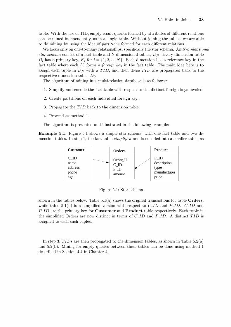
5.1 Holes in Joins 38
table. With the use of TID, empty result queries formed by attributes of different relationscan be mined independently, as in a single table. Without joining the tables, we are ableto do mining by using the idea of partitions formed for each different relations.
We focus only on one-to-many relationships, specifically the star schema. An N-dimensionalstar schema consist of a fact table and N dimensional tables, DN . Every dimension tableDi has a primary key, Ki for i = {1, 2, . . . N}. Each dimension has a reference key in thefact table where each Ki forms a foreign key in the fact table. The main idea here is toassign each tuple in DN with a TID, and then these TID are propagated back to therespective dimension table, Di.
The algorithm of mining in a multi-relation database is as follows::
1. Simplify and encode the fact table with respect to the distinct foreign keys involed.
2. Create partitions on each individual foreign key.
3. Propagate the TID back to the dimension table.
4. Proceed as method 1.
The algorithm is presented and illustrated in the following example:
Example 5.1. Figure 5.1 shows a simple star schema, with one fact table and two di-mension tables. In step 1, the fact table simplified and is encoded into a smaller table, as
Customer
C_IDnameaddressphoneage
Orders
Order_IDC_IDP_IDamount
Product
P_IDdescriptiontypesmanufacturerprice
Figure 5.1: Star schema
shown in the tables below. Table 5.1(a) shows the original transactions for table Orders,while table 5.1(b) is a simplified version with respect to C ID and P ID. C ID andP ID are the primary key for Customer and Product table respectively. Each tuple inthe simplified Orders are now distinct in terms of C ID and P ID. A distinct TID isassigned to each such tuples.
In step 3, TIDs are then propagated to the dimension tables, as shown in Table 5.2(a)and 5.2(b). Mining for empty queries between these tables can be done using method 1described in Section 4.4 in Chapter 4.
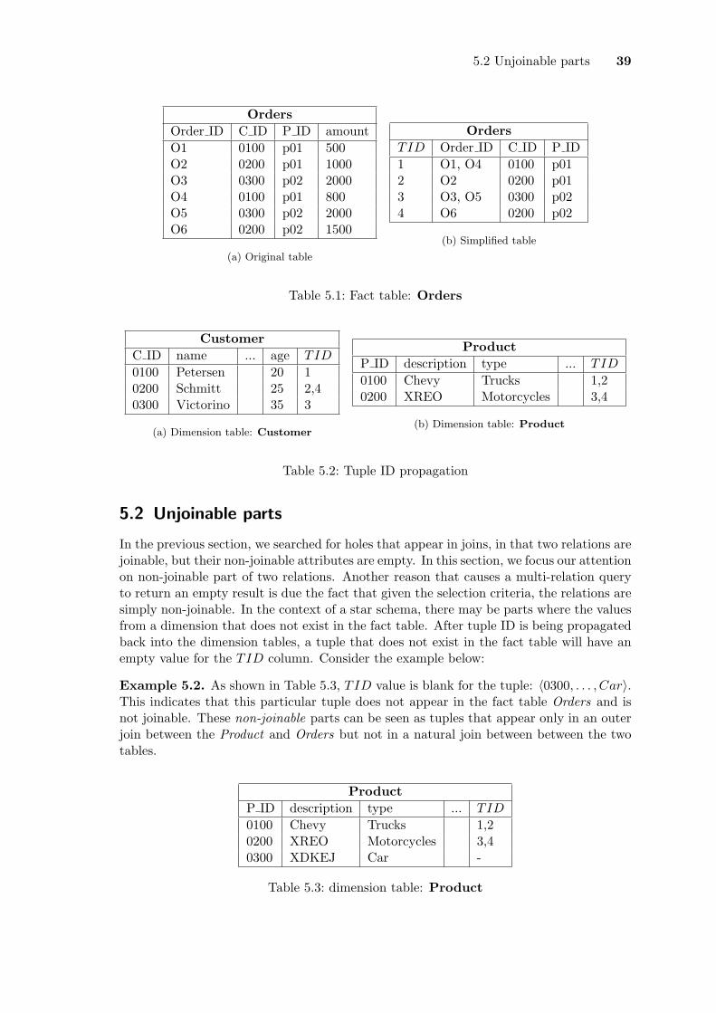
5.2 Unjoinable parts 39
OrdersOrder ID C ID P ID amountO1 0100 p01 500O2 0200 p01 1000O3 0300 p02 2000O4 0100 p01 800O5 0300 p02 2000O6 0200 p02 1500
(a) Original table
OrdersTID Order ID C ID P ID1 O1, O4 0100 p012 O2 0200 p013 O3, O5 0300 p024 O6 0200 p02
(b) Simplified table
Table 5.1: Fact table: Orders
CustomerC ID name ... age TID
0100 Petersen 20 10200 Schmitt 25 2,40300 Victorino 35 3
(a) Dimension table: Customer
ProductP ID description type ... TID
0100 Chevy Trucks 1,20200 XREO Motorcycles 3,4
(b) Dimension table: Product
Table 5.2: Tuple ID propagation
5.2 Unjoinable parts
In the previous section, we searched for holes that appear in joins, in that two relations arejoinable, but their non-joinable attributes are empty. In this section, we focus our attentionon non-joinable part of two relations. Another reason that causes a multi-relation queryto return an empty result is due the fact that given the selection criteria, the relations aresimply non-joinable. In the context of a star schema, there may be parts where the valuesfrom a dimension that does not exist in the fact table. After tuple ID is being propagatedback into the dimension tables, a tuple that does not exist in the fact table will have anempty value for the TID column. Consider the example below:
Example 5.2. As shown in Table 5.3, TID value is blank for the tuple: 〈0300, . . . , Car〉.This indicates that this particular tuple does not appear in the fact table Orders and isnot joinable. These non-joinable parts can be seen as tuples that appear only in an outerjoin between the Product and Orders but not in a natural join between between the twotables.
ProductP ID description type ... TID
0100 Chevy Trucks 1,20200 XREO Motorcycles 3,40300 XDKEJ Car -
Table 5.3: dimension table: Product

5.2 Unjoinable parts 40
Based on the above illustration, we now introduce the definition of the target domain.
Definition 5.1. Target domain. Target domain, target domain is the domain of anattribute based on the values that appear in the target table.
target dom(Ai) = t[i], t ∈ target table.
In a star schema, the target table is the fact table. The extended definition of an emptyvalue in the context of a star schema is:
Empty values : ai ∈ dom(Ai), ai /∈ target dom(Ai).
Example 5.3. Based on Example 5.2, the empty value for attribute type with respect tothe fact table Orders is ’Car’. The value ’Car’ belongs to dom(type) for dimension tableProduct, but does not exist in target dom(type). Any query to the fact table that has theselection criteria type =′ Car′ evaluates to empty.
6Test and Evaluation
In this section, we describe the experiments and the evaluation of the performance of theproposed solution. To get a more accurate evaluation, we evaluated the algorithm usingboth synthetic and real life datasets. They were obtained from WEKA machine learninghomepage [Witten and Frank, 2005]. Larger datasets were chosen to demonstrate thescalability of the proposed solution. A subset of all the attributes in each dataset wereselected, and the selection were based on the following criteria:
• discrete attributes: low cardinality (with cardinality below 10)
• continuous attributes: unrestricted range but different value distribution were chosento demonstrate the mining of EHR.
More description about each individual test can be found in the following sections.Besides that, we have conducted tests based on other factors, such as using different
values for threshold τ , varying distribution size and using the different combination ofdata types. In Chapter 4, we have focused mainly on mining EHR, but it is also shownthat the method can be used mine heterogeneous itemsets. All mined results are presentedin the form of rules. For rules that involves continuous attributes, they can be presentedin the form of empty rectangles. The visualization of some of the results in the form ofempty rectangles in two dimensional space will be presented in the result section.
Experimental Setup
The tests were ran on a personal computer with 1.6GHz processor, 1GB main memoryand Pentium 4 PC with Windows 2000. The proposed algorithm is implemented in Java.It is assumed that for all test cases, the simplified database Ds fits into the main memory.
6.1 Performance on Synthetic Datasets
TPCH
The TPC Benchmark H (TPC-H) is a decision support benchmark and it is a publiclyavailable workload, which allows for replication and for experiments. The attributes werechosen from two tables, namely orders and lineitems. This testset is stored in a DBMS.The join of these two tables has the size of 6,000,000 tuples and the initial dataset doesnot fit into the main memory. For the simplicity of the testing, the simplified database Ds
41
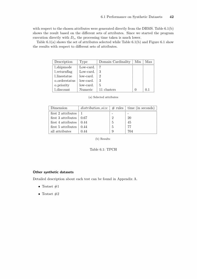
6.1 Performance on Synthetic Datasets 42
with respect to the chosen attributes were generated directly from the DBMS. Table 6.1(b)shows the result based on the different sets of attributes. Since we started the programexecution directly with Ds, the processing time taken is much lower.
Table 6.1(a) shows the set of attributes selected while Table 6.1(b) and Figure 6.1 showthe results with respect to different sets of attributes.
Description Type Domain Cardinality Min Maxl shipmode Low-card. 7l returnflag Low-card. 3l linestatue low-card. 2o orderstatus low-card. 3o priority low-card. 5l discount Numeric 11 clusters 0 0.1
(a) Selected attributes
Dimension distribution size # rules time (in seconds)first 2 attributes 1 - -first 3 attributes 0.67 2 20first 4 attributes 0.44 5 45first 5 attributes 0.44 5 77all attributes 0.44 9 704
(b) Results
Table 6.1: TPCH
Other synthetic datasets
Detailed description about each test can be found in Appendix A.
• Testset #1
• Testset #2
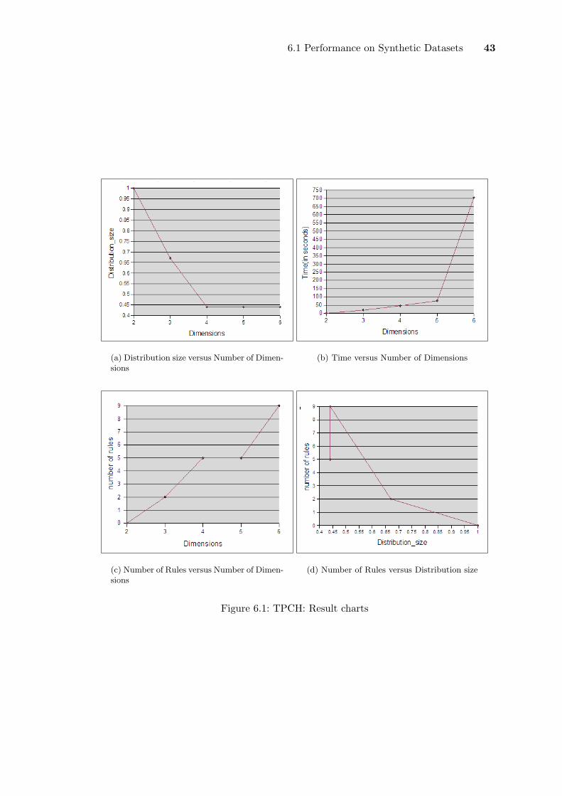
6.1 Performance on Synthetic Datasets 43
(a) Distribution size versus Number of Dimen-sions
(b) Time versus Number of Dimensions
(c) Number of Rules versus Number of Dimen-sions
(d) Number of Rules versus Distribution size
Figure 6.1: TPCH: Result charts

6.2 Performance on Real Life Datasets 44
6.2 Performance on Real Life Datasets
Table 6.2 below is the testset for California Housing Survey, with the size of 20,640 tuples,obtained from the StatLib repository (http://lib.stat.cmu.edu/datasets/). It contains in-formation on housing survey on all the block groups in California from the 1990 Census.
Description Type Domain Cardinality min maxMedian Age Numeric 52 clusters 1 52Total # rooms Numeric 56 clusters 2 39320total # bedrooms Numeric 59 clusters 1 6445Household Numeric 65 clusters 1 6,082Median Income Numeric 76 clusters 0.5 15Median House Value Numeric 86 clusters 14,999 500,001
(a) Selected attributes
Dimension distribution size # rules time (in seconds)first 2 attributes 0.53 106 218first 3 attributes 0.38 389 532first 4 attributes 0.2 1,825 645first 5 attributes 0.17 2,180 3268all attributes 0.08 6,686 4,842
(b) Results
Table 6.2: California House Survey
Other real life datasets
Detailed description about each test can be found in Appendix A.
• Ailerons
• Credit Card Approval
• KDD Internet usage survey

6.2 Performance on Real Life Datasets 45
(a) Distribution size versus Number of Dimen-sions
(b) Time versus Number of Dimensions
(c) Number of Rules versus Number of Dimen-sions
(d) Number of Rules versus Distribution size
Figure 6.2: California House Survey: Result charts
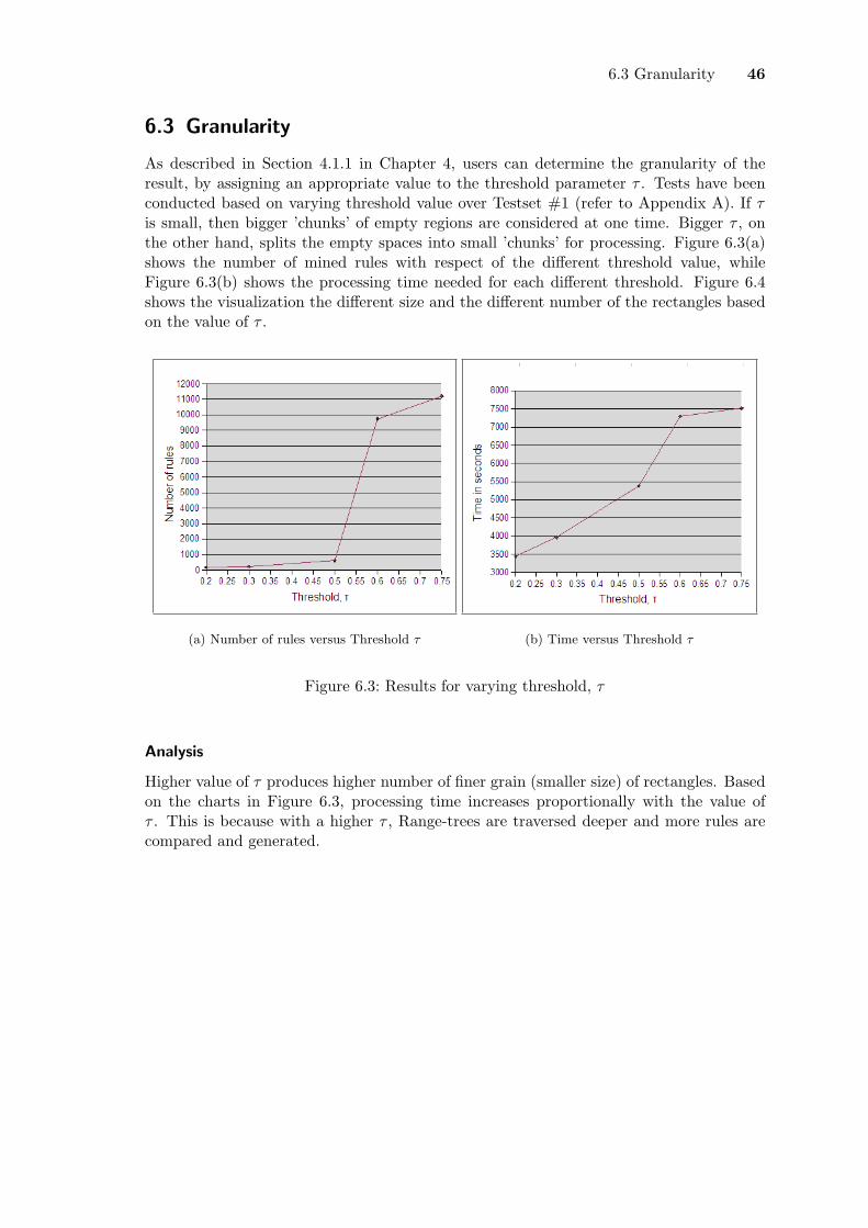
6.3 Granularity 46
6.3 Granularity
As described in Section 4.1.1 in Chapter 4, users can determine the granularity of theresult, by assigning an appropriate value to the threshold parameter τ . Tests have beenconducted based on varying threshold value over Testset #1 (refer to Appendix A). If τis small, then bigger ’chunks’ of empty regions are considered at one time. Bigger τ , onthe other hand, splits the empty spaces into small ’chunks’ for processing. Figure 6.3(a)shows the number of mined rules with respect of the different threshold value, whileFigure 6.3(b) shows the processing time needed for each different threshold. Figure 6.4shows the visualization the different size and the different number of the rectangles basedon the value of τ .
(a) Number of rules versus Threshold τ (b) Time versus Threshold τ
Figure 6.3: Results for varying threshold, τ
Analysis
Higher value of τ produces higher number of finer grain (smaller size) of rectangles. Basedon the charts in Figure 6.3, processing time increases proportionally with the value ofτ . This is because with a higher τ , Range-trees are traversed deeper and more rules arecompared and generated.

6.3 Granularity 47
(a) τ = 0.5, x-axis: X6, y-axis: X4
(b) τ = 0.75, x-axis: X6, y-axis: X4
Figure 6.4: Mined EHR based on different threshold, τ

6.4 Varying Distribution Size 48
6.4 Varying Distribution Size
Recall that in Section 4.3 in Chapter 4, data distribution is measured in terms of distribution size.The choice of running method 1 or method 2 is determined by the distribution size. Asynthetic dataset was generated based on a fixed set of attributes, but with varying dis-tribution size. The list of attributes are listed in Table 6.3.
Description Type Domain Cardinalityatt1 low-card. 5att2 low-card. 5att3 numeric 25 clustersatt4 numeric 15 clustersatt5 low-card. 5
Table 6.3: Synthetic datasets
Analysis
The result for different distribution size is displayed in Figure 6.5. From the resultsshown in Figure 6.5(a), we are able to draw the conclusion that the time is proportionalto distribution size. As for the number of mined rules, it does not depend on datadistribution, as displayed in Figure 6.5(b).
(a) Time versus Distribution Size (b) Number of Rules versus Distribu-tion Size
Figure 6.5: Results for varying distribution size over a fixed set of attributes
6.5 Different Data Types
These test datasets are chosen to show the working for the algorithm in the case of ho-mogeneous and heterogeneous data types (a mixture of categorical and numerical values).For categorical values, they are of low cardinality domain, while for numeric values, they
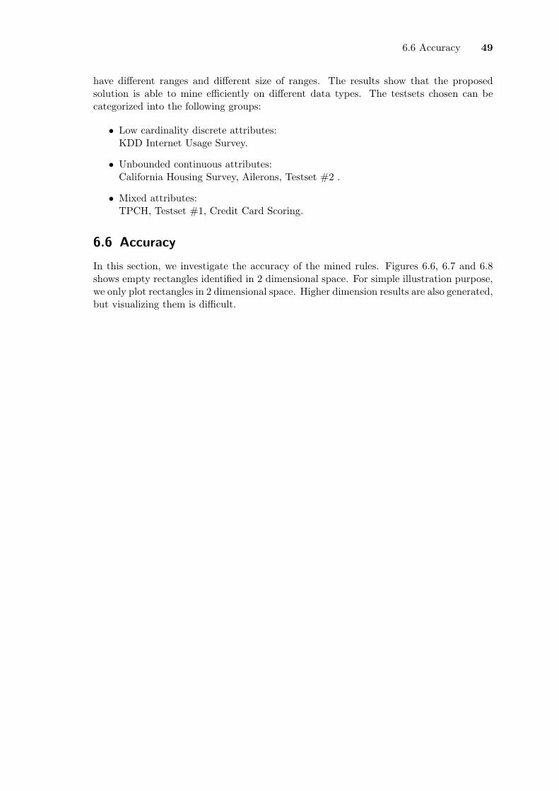
6.6 Accuracy 49
have different ranges and different size of ranges. The results show that the proposedsolution is able to mine efficiently on different data types. The testsets chosen can becategorized into the following groups:
• Low cardinality discrete attributes:KDD Internet Usage Survey.
• Unbounded continuous attributes:California Housing Survey, Ailerons, Testset #2 .
• Mixed attributes:TPCH, Testset #1, Credit Card Scoring.
6.6 Accuracy
In this section, we investigate the accuracy of the mined rules. Figures 6.6, 6.7 and 6.8shows empty rectangles identified in 2 dimensional space. For simple illustration purpose,we only plot rectangles in 2 dimensional space. Higher dimension results are also generated,but visualizing them is difficult.

6.6 Accuracy 50
(a) (x-axis: median house value, y-axis: total # rooms)
(b) (x-axis: Median Age, y-axis: Median Income)
Figure 6.6: Point distribution and EHR [California Housing Survey]
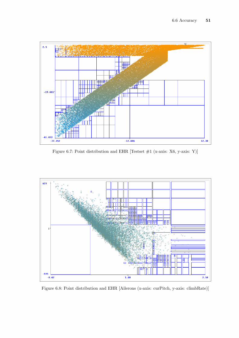
6.6 Accuracy 51
Figure 6.7: Point distribution and EHR [Testset #1 (x-axis: X6, y-axis: Y)]
Figure 6.8: Point distribution and EHR [Ailerons (x-axis: curPitch, y-axis: climbRate)]

6.7 Performance Analysis and Summary 52
6.7 Performance Analysis and Summary
In this method, false positives are not allowed while false negatives are tolerable. That is,all mined rules are guaranteed to be empty, but there may be empty regions in the datasetwhich are not mined. This is due to two factors:
1. User defined coverage, τ . This parameter determines the granularity of the minedhyper-rectangles. The bigger the value of τ , the more accurate the results will be.If the value of τ is small, lesser rules are obtained and the accuracy of the minedresult will be sacrificed.
2. Clusters are defined to be as small as possible, but since it is not feasible to havea cluster for each and every individual point, there will be empty region within thecluster itself. In this case, we treat a cluster as a totally filled region, and thereforemisses the empty spaces within the cluster. However, since the points in a clusterfalls within the interval threshold T , the empty spaces within the cluster will havethe size of less than T . Therefore these regions are small enough to be ignored.
6.7.1 Comparison to existing methods
Since the approach of this method is different from any existing method, there is no directand clear cut comparison to any of the existing methods. Nevertheless, comparisons canstill be made in terms of strengths and limitations. The existing methods mentioned hereare with reference to ones discussed in detail in Chapter 2.
In the method outlined in [Edmonds et al., 2001], uses the concept of growing emptyrectangles. They depict the dataset as an |X| × |Y | matrix of 0’s and 1’s. To obtainthe largest possible rectangles or maximal rectangles, the data has to be sorted first, sothat all 0’s are in the adjacent position. Many smaller isolated holes are not taken intoconsideration. In our case, isolated empty regions can be mined without sorting the datapoints first. With just one pass of the database, the Range-trees can be constructed. Asshown in Section 6.6, it is evident that the algorithm is able to detect empty spaces ofdifferent shapes and sizes.
From the test results, we demonstrated that the algorithm works well for both discreteand continuous attributes. Both methods that discover holes by geometry ([Edmondset al., 2001] and [Liu et al., 1997])has the limitation of working only on continuous values.The method using Decision Tree induction [Liu et al., 1998] is able to cater for bothdiscrete and continuous attributes, but focuses only on the latter.
All existing methods (except [Luo, 2006]) focus only finding empty rectangles in twodimensional spaces, and they do not perform well in higher dimensional spaces becauseof high time and space complexity. In this case, we have shown that this method scaleswell in higher dimension spaces. Here tests and experiments of 4 to 7 dimensions wereconducted. The method can be accommodated to mine higher dimensional by storing andwriting data on disk as suggested in Section 6.7.3.
6.7.2 Storage and Scalability
This method scales well to large database as the algorithm runs independently on thesize of the original dataset, but dependent only on max set, which is determined by thedomains of the set of chosen attributes. The description and calculation of max set isfound in 4.1.3 in Chapter 4. First we do a simplification encoding of the database, toobtain Ds. The size of the simplified database Ds has the upper bound of the size of

6.7 Performance Analysis and Summary 53
max set. In most cases, |Ds| is much smaller than |max set| unless the dataset is denselypopulated and evenly spread out.
Both method 1 an 2 uses the levelwise search, they can be analaysed as follows: In theworst case analysis, the time and space complexity depends on the number of sets in thelevels Ll, called the size of a level. Let n be the number of dimensions and s be the sumof the sizes of the levels. In the worst case, s = O(2n).
During the generation of Ck, we need storage for Lk−1 and the candidates Ck (In thecase of method 2, for the generation of Ck, we need storage for Lk+1). Memory needs tobe managed carefully as the candidates generation phase may occupy and take up all theavailable buffer. When the distribution size is large, candidate generation may run intothe problem of insufficient main memory. To overcome this problem, method 2 is proposedas an alternative to deal with datasets with large distribution size.
The two main differences between method 1 and 2 are outlined as follows:
• Disk Access: In method 1, it needs O(|Ds|) access, while for method 2, it needs O(s)accesses of size O(|Ds|).
• Main Memory Requirement: Method 1 requires higher storage space, because besidesstoring the Lk and Ck+1, extra storage space are needed for idlist. In the worst case,the space complexity is O(2n |idlist|). As for method 2, it needs storage space of Lk
and Ck−1. In the worst case, the space complexity is O(2n).
6.7.3 Buffer Management
The method employed here is independent of the dataset size, but with a upper boundof the maximal set, max set (the cross product of the attribute domains.) Therefore thisalgorithm works well for attributes with low cardinality domains.
Method 1:
In the candidate generation phase of pass k, we need storage for itemset Lk−1 (includingtheir TID)and the candidate itemset Ck. If Lk−1 does not fit into the memory, we exter-nally sort Lk−1. We bring into memory a block of Lk−1 in which the first k − 2 items arethe same. We now generate candidates using this block. We are interested in the prunedoff itemsets, those itemset where their combination of Lk−1 does not have any commonTID and produces an empty set intersection. They are paged out onto disk as results.
Method 2:
We start off with Ln, with n dimensions. In the candidate generation phase of pass k, weneed storage for itemsets Lk and the candidate Ck−1. In the dataset scanning phase, weneed storage for Ck and at least one page to buffer the database transaction. Lk are storedand paged out onto disk if memory is insufficient. Testing for minimality and pruning willbe done once the levelwise algorithm is finished. An efficient test for minimality can bedone using a hashtable.

6.7 Performance Analysis and Summary 54
6.7.4 Time Performance
Time performance in each step of the methods are analyzed as follows:
Step 1: Data Preprocessing
In the data preprocessing phase, values in continuous attributes are clustered. Let m bethe number of continuous attributes. In the data preparation phase, the algorithm needsto scan through the original dataset, D with |D| tuples. Each data tuple may travel atmost logB |D| steps down a Range-tree, where B is the branching factor of an internal nodein the Range tree. All the above operations are duplicated for each of the m dimensionsgiving a time complexity of O(m |D| (logB |D|)).
Step 2: Simplify Database
In this step, we simplify the database into a smaller dataset Ds. We need to access theoriginal dataset, the time complexity is linear to the number of tuples in the originaldataset, which is O(|D|). The process of simplifying the database is done using the hashtable. Each unique tuples is stored in a hashtable, while non-unique tuples are ignored.The process of checking whether a tuple is unique can be done in constant time by checkingfor the entries in the hashtable.
Step 3: Method 1
In method 1, candidates Ck are created by testing for non-empty set intersection idlist ofLk−1. The checking of set intersection between two idlist is polynomial. Let l1 be |idlist1|and l2 be |idlist2|, the time complexity is O(l1l2). Since we store the TID in main memory,there is no need to scan the database for each level, thus it is faster. However the downsideof this method is that it incurs a higher storage space.
Step 3: Method 2
For this, we need to scan the database for every level in the lattice, hence the access timeis slow. One of the main advantages is the linear dependency of the algorithm on thenumber of rows in the relation and linear to the size of the number of attributes. Afterthat, all non-minimal empty combinations are eliminated. Method 2 does not incur highstorage space, but requires a longer run time.
6.7.5 Summary
The method is at its best when the number of attribute in an Lempty are relatively small.When the size of the empty rules is roughly one half of the number of attributes, thenumber of itemset is exponential in the number of attributes. When the attribute com-binations are larger than that, the levelwise method that starts the search from smalldependencies obviously is further from the optimum. In this situation, we apply method2, which starts from the largest combination and work our way to smaller combinations.
Here is the observation made, the distribution size is inversely proportional to thenumber of dimension. It is found that distribution size decreases as more attributesare being considered. This is consistent with the observation made in [Agrawal et al.,1998], where it is stated that the average density of points in a high dimensional spaceis likely to be quite low. Therefore, they propose first to mine dense region in lowersubspace, before proceeding higher dimensional spaces. From all the expriments and the
6.7 Performance Analysis and Summary 55
corresponding results, it is found that distribution size is generally quite small when itinvolves continuous attributes. Consequently in most cases, method 1 is used.
In view of the time and space complexity of both method 1 and 2, it is thereforejustifiable to use both methods as a more robust method for mining EHR in differentdata distribution. By taking into consideration of the data distribution, we can finda suitable method that will ensure a method that has an efficient runtime and storagespace.
6.7.6 Practical Analysis
Due to pruning, s can be significantly smaller than the worst case analysis. In the can-didate generation phase, Lk are stored in hashtable, making pruning of Ck+1 at constanttime. For the elimination of non-minimal empty combination, mined rules are stored inhashtables. Therefore, in practice, the retrieval and pruning of rules takes constant time.
6.7.7 Drawbacks and Limitations
One of the drawbacks of the algorithm is that for some cases, a large number of rules areproduced. In cases like these, it will simply be counter-productive if the number of rulesare almost equal or close to the size of the dataset. This is because a large amount oftime has to be devoted to check through the rules to determine whether any given query isempty. Besides that, a large storage space is needed to store the rules. In such situation,mining and checking for empty result queries will incur a high computational cost.
The size of the rectangles depends on the types of data distribution. Clusters for eachcontinuous attributes are formed according to the positions of points, where points locatedin close proximity to each other forms a cluster. For points that are highly skewed, biggersized rectangles can be identified (refer Figure 6.8, 6.7), whereas for points that are evenlydistributed, clusters of equal size and are located close to each other are produced. In factin such cases, no real clusters are formed since the data points are evenly scattered. (eg:Figure 6.6(b)). In this case, rectangles are that small or insignificant are produced. Thiscan be explained using the concept used in [Liu et al., 1997]. A maximal hyper-rectangleis split when a data point is added. The existing rectangles are repeatedly being split intosmaller rectangles whenever a new data point is added. If the point distribution is evenlyscattered, then many small rectangles will be produced. Analogous in our situation, minedrules produced have a very fine granularity and are not useful in empty query detection.To overcome this problem, [Liu et al., 1997] proposed to mine only sufficiently large emptyregions.

7Integration of the algorithms into query processing
In this chapter, we explore the potential usage of mined EHR. First and foremost, we canuse it to detect empty result queries. This is done by matching the selection criteria withthe mined rules. Once any selection criteria is found to be an exact match or a supersetof any empty rules, then that particular query is categorized as ’empty’ and thus will notbe evaluated. All EHR can be materialized as views, as described in [Gryz and Liang,2006]. Another alternative is to store them in the form of rules.
7.1 Different forms of EHR
As explained earlier, mining of empty result queries can be done in the form of findingempty spaces in datasets or selection rules. The goal is to mine the minimum empty querycombination Lk−empty, and any superset of an empty selection will not be stored.
Mined rules.
Mined rules are stored in a Disjunctive Normal Form (DNF). Queries that matches one ofthe clauses will be categorized as empty. The rules are stored in the following form:
Lempty : {rule1 ∨ rule2 ∨ . . . rulem}
where rulei for i ∈ {1, . . . m} is in the form of Conjunctive Normal Form(CNF), consistingof
• point based comparison (for discrete and continuous attributes): Ax = ax
• interval comparison (for continuous attributes): minx ≤ Ax ≥ maxx
where Ax ∈ A, and x ∈ {1, . . . , n}.
Example 7.1. Let D be a database with attributes A = {A1, A2, A3}, where A1, A2 arecontinuous valued attributes and A3 is a discrete valued attribute, with the domain of{a31 , a32 , a33}.rule1: 5 < A1 < 10rule2: 2 < A2 < 14 ∧A3 = a33
rule3: 13 < A1 > 20 ∧ 15 < A2 < 20 ∧A3 = a31
56

7.2 Avoid execution of empty result queries 57
The mined rules are presented in this form:
Lempty = (5 < A1 < 10)∨ (2 < A2 < 14 ∧A3 = a33)∨ (13 < A1 > 20 ∧ 15 < A2 < 20 ∧A3 = a31)
Materialized Views
As for finding empty regions in the data, it is analogous to finding empty hyper-rectangles.The mined results can be materialized as views. When a materialized view for a set ofattributes X is constructed, all empty rules of set X and all rules involving subset of X arecombined to form the view. In the visualized form, all EHR formed by the subset of X,which are in lower dimension are projected to X dimensions.
Both rules and materialized views can be used in detecting empty result queries. Minedrules can be used in the form of checking against the selection criteria of a query. If thequery selection matches any of the conjunctive clauses, then it is categorized as ’empty’.EHR can be materialized as views. Any query that falls within the empty region definedby the EHR is categorized as ’empty’.
7.2 Avoid execution of empty result queries
Our main focus here is to detect these empty result queries and to avoid executing them.A possible implementation of empty query detection can be done for ’canned queries’.’Canned queries’ are predefined queries, with predefined selection predicates. In mostinstances, canned queries contain prompts that allows user to select the query parametersfrom a list. In these cases, only the selection values in the query changes. Typically,these kind of queries are common for end users in the Internet domain. Online users oftensubmit canned queries by filling parameter values into a predefined template. This usuallyinvolves choosing a few predefined lists, each having a low cardinality domain. An examplewould be the Advanced Online Search, that has more selection criteria than a general orbasic search.
We propose to use mined EHR in this context. Since the method that we proposeefficiently mines low cardinality domains, we can use the result in detecting empty cannedqueries. We output EHR in the form of rules and populate them in the form of an XMLfile. The XML file can then be placed in the intermediate stage to check for empty resultqueries before queries are being sent to DBMS to be evaluated. Figure 7.1 shows thearchitecture.
Internet Data source
Mined rules (XML file)
User query
Figure 7.1: Implementing mined empty queries for online queries

7.2 Avoid execution of empty result queries 58
These XML files are generated according to the following DTD, shown in Table 7.1. Anexample of such an XML file is shown in Table 7.2.
<!DOCTYPE emptySets [<!ELEMENT emptySets (emptySet*)><!ELEMENT emptySet (rule_no, att1?, att2?,....attn?)><!ELEMENT att1 (#PCDATA)><!ELEMENT att2 (#PCDATA)>..<!ELEMENT attn (#PCDATA)>
]>
Table 7.1: DTD
<?xml version="1.0"?><emptySets">
<emptySet><rule_no>1</rule_no><att1>A</att1>
</emptySet><emptySet>
<rule_no>2</rule_no><att2>
<min>5</min><max>10</max>
</att2></emptySet><emptySet>
<rule_no>3</rule_no><att1>B</att1><att2>
<min>15</min><max>20</max>
</att2></emptySet>
</emptySets>
Table 7.2: An example of an XML file
Query criteria matching can be done using XQuery FLOWR expression. Table 7.3 showsan example of XQuery used in respect to the XML file in Table 7.2:
If the XQuery evaluates to true and returns an XML node, then we know that theselection criteria of the query matches the empty rules. If no match is found, then querywill be sent to the DBMS.

7.3 Interesting Data Discovery 59
for $x in doc("empty.xml")/emptySets/emptySetwhere $x/att1=’A’
or ($x/att2/min=5 and $x/att2/max<15)return $x/number
Table 7.3: XQuery
Two applications were proposed in [Gryz and Liang, 2006]. They are:
1. Query optimization by query rewritingEmpty hyper-rectangles can be materialized in views and used for query optimiza-tion. By reducing the range of one or more of the attributes or by adding a rangepredicate (hence reducing an attributes range), the number of tuples that participatein the join execution are reduced thus providing optimization.
2. Improve Cardinality estimates in query processingCurrently, a join cardinality estimate is based on the assumption of uniform datadistribution or by using histogram. By identifying and taking into consideration theempty regions in a join, the corresponding join cardinality estimate is more accurate.
7.3 Interesting Data Discovery
Clearly, the knowledge of empty regions may be valuable in and of itself as it may revealunknown correlations between data values which can be exploited in applications. Asdescribed earlier, empty regions in data can be seen as a type of data skew. From themined empty regions, it can lead to interesting data discovery, for example attributecorrelations and functional dependencies.
In [Liu et al., 1997], the authors proposed to use the knowledge of empty regions inmedical domains. For example, in a disease database, we may find that certain symtomsand/or test values do not occur together, or when a certain medicine is used, some testvalues never go beyond certain range. Discovery of such information can be of greatimportance in medical domains because it could mean the discovery of a cure to a diseaseor even some biological laws.
7.4 Other applications
1. Database administrationThe knowledge of empty regions can help database administrator in adding integrityconstraint or check constraint in the database.
2. Detection of anomalies in updatesFrom the mined rules, we are able to identify which ranges of values do not occurtogether. They can be used in checking for anomalies in updates.
8Conclusion
The results have shown that given a set of attributes, the proposed solution is able tofind the set of empty combination in the query selection that causes a particular query toreturn an empty result. The mined results are presented as disjunction of rules. In thespecial case of numeric attributes, these rules can be defined in terms of empty hyper-rectangles. The proposed solution has a few strong points over existing methods. Unlikeprevious methods, they focus only in finding empty regions formed by numeric values, thismethods explores the combinations of category and numeric values. Besides being able tomine mixed type of attributes, it can also mine hyper-rectangles in higher dimensions. Itis shown that the algorithm is independent of the size of the actual dataset but dependentonly on the size of the attribute domains. It is efficient for low cardinality domains, butperformance degrades if the cardinality of the attribute domains becomes too large. In thismethod, false positive are allowed, but no false negatives are reported. This means thatall mined rules are guaranteed to be ’empty’, however there may be some empty regionsthat go undetected. Since this solution has good performance for low cardinality domains,therefore it can be implemented to detect empty query results for ’canned queries’.
8.1 Future Work
We expect this feature of mining empty result queries to be most helpful in read-mostlyenvironments. Extending this to a more update-intensive environment is an interestingarea for future work. The continuation of this work would be to use the mined results toefficiently detect empty result queries. As stated, there exist a few previous works thatcheck for empty regions in the dataset, however only [Luo, 2006] focused on empty resultqueries detection.
Section 6.7.7 in Chapter 6 contains the list of drawbacks and limitation of the proposedmethod. One of them is that the mined rules are too fragmented to be useful in emptyquery detection. Thus, it is worth investigating on how to optimize the current rules,by combining these ’fragments’, making them large enough to be used in empty querydetection. By combining these ’fragmented’ rules, we can minimize the number of rulesused to define empty spaces. This optimization problem of finding the minimal numberof rules to fully identify the empty regions is known to be NP-Hard. Just like it is statedin [Agrawal et al., 1998], computing the optimal cover is also NP-hard. Nonetheless, itwill be interesting to see the performance of empty query detection in such optimizedcondition.
60

Bibliography
R. Agrawal and R. Srikant. Fast algorithms for mining association rules. In J. B. Bocca,M. Jarke, and C. Zaniolo, editors, Proc. 20th Int. Conf. Very Large Data Bases, VLDB,pages 487–499. Morgan Kaufmann, 12–15 1994. ISBN 1-55860-153-8. URL citeseer.ist.psu.edu/agrawal94fast.html. 4.4, 4.4.2
R. Agrawal, J. Gehrke, D. Gunopulos, and P. Raghavan. Automatic subspace cluster-ing of high dimensional data for data mining applications. pages 94–105, 1998. URLciteseer.ist.psu.edu/agrawal98automatic.html. 2.2.3, 3.2.1, 6.7.5, 8.1
Q. Cheng, J. Gryz, F. Koo, T. Y. C. Leung, L. Liu, X. Qian, and K. B. Schiefer. Im-plementation of two semantic query optimization techniques in db2 universal database.In VLDB ’99: Proceedings of the 25th International Conference on Very Large DataBases, pages 687–698, 1999. 1
S. S. Cosmadakis, P. C. Kanellakis, and N. Spyratos. Partition semantics for relations. InJournal Computer System Science, pages 203–233, 1986. 4.4.1
J. Edmonds, J. Gryz, D. Liang, and R. J. Miller. Mining for empty rectangles in largedata sets. In ICDT, pages 174–188, 2001. 2.1, 2.2.2, 3.1, 6.7.1
T. Fukuda, Y. Morimoto, S. Morishita, and T. Tokuyama. Data mining using two-dimensional optimized association rules: scheme, algorithms, and visualization. InSIGMOD ’96: Proceedings of the 1996 ACM SIGMOD international conference onManagement of data, pages 13–23, New York, NY, USA, 1996. ACM. ISBN 0-89791-794-4. doi: http://doi.acm.org/10.1145/233269.233313. 3.2.1
J. Gryz and D. Liang. Holes in joins. In J. Intell. Inf. Syst., volume 26, pages 247–268,Hingham, MA, USA, 2006. Kluwer Academic Publishers. doi: http://dx.doi.org/10.1007/s10844-006-0368-2. 1, 1.1, 2.2.2, 3.1, 5.1, 7, 7.2
Y. Huhtala, J. Kinen, P. Porkka, and H. Toivonen. Efficient discovery of functionaland approximate dependencies using partitions. In ICDE, pages 392–401, 1998. URLciteseer.ist.psu.edu/huhtala97efficient.html. 4.4.1
W. Kießling and G. Kostler. Preference sql - design, implementation, experiences. InVLDB, pages 990–1001, 2002. 1.1
B. Lent, A. Swami, and J. Widom. Clustering association rules. In ICDE, 1997. URLmack.ittc.ku.edu/lent97clustering.html. 4.1.2
B. Liu, L.-P. Ku, and W. Hsu. Discovering interesting holes in data. In IJCAI (2), pages930–935, 1997. 2.1, 2.2.2, 2.2.2, 2.2.3, 6.7.1, 6.7.7, 7.3
61

BIBLIOGRAPHY 62
B. Liu, K. Wang, L.-F. Mun, and X.-Z. Qi. Using decision tree induction for discoveringholes in data. In Pacific Rim International Conference on Artificial Intelligence, pages182–193, 1998. URL citeseer.ist.psu.edu/liu98using.html. 2.1, 2.2.2, 6.7.1
G. Luo. Efficient detection of empty-result queries. In VLDB, pages 1015–1025, 2006. 1.1,2.2.1, 6.7.1, 8.1
R. J. Miller and Y. Yang. Association rules over interval data. In J. Peckham, editor,SIGMOD 1997, Proceedings ACM SIGMOD International Conference on Managementof Data, May 13-15, 1997, Tucson, Arizona, USA, pages 452–461. ACM Press, 1997.4.2
D. J. Newman, S. Hettich, C. L. Blake, and C. J. Merz. UCI repository of machine learningdatabases, 1998. URL http://www.ics.uci.edu/~mlearn/MLRepository.html. A.2,2
N. Spyratos. The partition model: a deductive database model. In ACM Trans. DatabaseSyst., pages 1–37, 1987. 4.4.1
R. Srikant and R. Agrawal. Mining quantitative association rules in large relational tables.In H. V. Jagadish and I. S. Mumick, editors, Proceedings of the 1996 ACM SIGMODInternational Conference on Management of Data, pages 1–12, 1996. URL citeseer.ist.psu.edu/srikant96mining.html. 4.2
I. H. Witten and E. Frank. WEKA data mining: Practical machine learning tools andtechniques, 2005. URL http://www.cs.waikato.ac.nz/~ml/weka/. 6, 1, 2, 1, 3
X. Yin, J. Han, J. Yang, and P. Yu. Crossmine: Efficient classification across multipledatabase relations. 2004. URL citeseer.ist.psu.edu/yin04crossmine.html. 5.1
T. Zhang, R. Ramakrishnan, and M. Livny. BIRCH: an efficient data clustering methodfor very large databases. In ACM SIGMOD International Conference on Managementof Data, pages 103–114, Montreal, Canada, June 1996. URL citeseer.ist.psu.edu/article/zhang96birch.html. 4.2

AMore Test Results
A.1 Synthetic Dataset
1. Testset #1
• Description: artificial dataset with 6 attributes (3 discrete and 3 continuous).Data are generated with dependencies between the attribute values.
• Size of dataset: 40,768 rows of records
• Source: collection of regression datasets at WEKA dataset repository [Wittenand Frank, 2005].
Description Type Values Domain Cardinality min max
X3 Low cardinality brown, red, green 3X4 Numeric integer 61 clusters -7.5 2.5X6 Numeric integer 78 clusters -37.194 12.114X7 Boolean yes/no 2X8 Low cardinality normal, large 2Y Numeric integer 79 clusters -41.822 2.5
(a) Attributes of testset #1
Dimension distribution size # rules time (in seconds)
first 2 attributes 0.34 44 910first 3 attributes 0.22 423 2,895first 4 attributes 0.19 1,133 6,592first 5 attributes 0.19 1,216 14,140all attributes 0.08 34,772 31,322
(b) Results
Table A.1: Testset #1
63
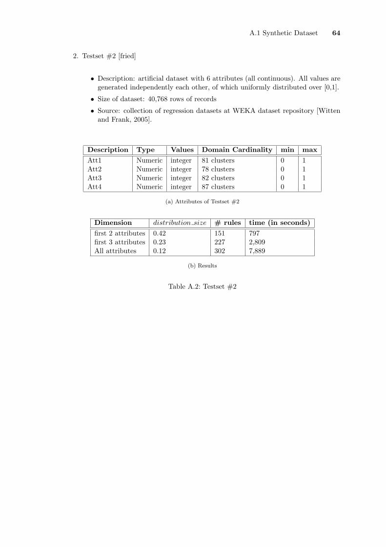
A.1 Synthetic Dataset 64
2. Testset #2 [fried]
• Description: artificial dataset with 6 attributes (all continuous). All values aregenerated independently each other, of which uniformly distributed over [0,1].
• Size of dataset: 40,768 rows of records
• Source: collection of regression datasets at WEKA dataset repository [Wittenand Frank, 2005].
Description Type Values Domain Cardinality min max
Att1 Numeric integer 81 clusters 0 1Att2 Numeric integer 78 clusters 0 1Att3 Numeric integer 82 clusters 0 1Att4 Numeric integer 87 clusters 0 1
(a) Attributes of Testset #2
Dimension distribution size # rules time (in seconds)
first 2 attributes 0.42 151 797first 3 attributes 0.23 227 2,809All attributes 0.12 302 7,889
(b) Results
Table A.2: Testset #2

A.2 Real Life Dataset 65
A.2 Real Life Dataset
For evaluation of real datasets, we have chosen a few datasets from UCI KDD (KnowledgeDiscovery in Databases) [Newman et al., 1998] and from statlib of CMU. Datasets fromboth these sources are provided in WEKA machine learning homepage.
1. Ailerons
• Description: This data set addresses a control problem, namely flying a F16aircraft. The attributes describe the status of the aeroplane.
• Size of dataset: 13,750 rows of records
• Source: collection of regression datasets at WEKA dataset repository [Wittenand Frank, 2005].
Description Type Values Domain Cardinality min max
climbRate Numeric integer 76 clusters -975 977q Numeric integer 58 clusters -0.54 0.62curPitch Numeric integer 71 clusters -0.42 2.58curRoll Numeric integer 61 clusters -3.1 2.9absRoll Numeric integer 21 clusters -23 -3diffDiffClb Numeric integer 53 clusters -62 46
(a) Attributes of Ailerons
Dimension distribution size # rules time (in seconds)
first 2 attributes 0.24 5 101first 3 attributes 0.18 683 420first 4 attributes 0.12 1,222 916first 5 attributes 0.09 3,404 1,907all attributes 0.04 11,268 4,016
(b) Results
Table A.3: Ailerons

A.2 Real Life Dataset 66
2. KDD internet usage
• Description: This data comes from a survey conducted by the Graphics andVisualization Unit at Georgia Tech in 1997. The particular subset of the surveyprovided here is the ”general demographics” of Internet users.
• Size of dataset: 10,108 rows of record
• Source: UCI KDD [Newman et al., 1998]
Description Type Values Domain Cardinality
Community Building Low-card. {D, E, L, M} 4Gender Boolean {Female, Male} 2Household Income Low-card. {[10-19], [20-29], [30-39], [40-
49], [50-59], [75-99], Nil,Over100}
9
Occupation Low-card. {Computer, Education, Man-agement, Other, Professional}
5
Marital Status Low-card. {Divorced, Married, Not Say,Other, Separated, Single,Widowed}
7
Race Low-card. {Asian, Black, Hispanic, In-degenous, Latino, Not Say,Others}
8
Years on internet Low-card. {1-3Yr, 4-6Yr, 6-12Yr,Over7Yr, Under6Mth}
5
(a) Attributes of KDD Internet Usage
Dimension distribution size # rules time (in seconds)
first 2 attributes 1 - -first 3 attributes 0.97 1 33first 4 attributes 0.95 32 77first 5 attributes 0.53 592 181first 6 attributes 0.11 2,524 755all attributes 0.04 6,987 7,800
(b) Results
Table A.4: KDD Internet Usage Survey

A.2 Real Life Dataset 67
3. Credit Card Scoring
• Description: Credit card application and approval based on application scoring.
• Size of dataset: 5,000 rows of records
• Source: collection of regression datasets at WEKA dataset repository [Wittenand Frank, 2005].
Description Type Values Domain Cardinality min max
Age Numeric integer 22 clusters 20 50Income Numeric integer 28 clusters 1.51 10Monthly CC expenditure Numeric integer 15 clusters 0 1898.03Own a home Boolean {yes / no} 2Category scoring low-card. {0,1,2,3,4,7} 6
(a) Attributes of Credit Card Scoring
Dimension distribution size # rules time (in seconds)
first 2 attributes 0.34 16 48first 3 attributes 0.12 30 193first 4 attributes 0.10 30 283All attributes 0.08 51 384
(b) Results
Table A.5: Credit Card Scoring