data mining, data warehousing and knowledge discovery basic algorithms and concepts srinath...
TRANSCRIPT

Data Mining, Data Warehousing and
Knowledge DiscoveryBasic Algorithms and Concepts
Srinath SrinivasaIIIT [email protected]

Overview
• Why Data Mining? • Data Mining concepts • Data Mining algorithms
– Tabular data mining– Association, Classification and
Clustering– Sequence data mining– Streaming data mining
• Data Warehousing concepts

Why Data MiningFrom a managerial perspective:
Strategic decision making
Wealth generation
Analyzing trends
Security

Data Mining
• Look for hidden patterns and trends in data that is not immediately apparent from summarizing the data
• No Query…
• …But an “Interestingness criteria”

Data Mining
+ =Data
Interestingnesscriteria
Hiddenpatterns

Data Mining
+ =Data
Interestingnesscriteria
Hiddenpatterns
Type of Patterns

Data Mining
+ =Data
Interestingnesscriteria
Hiddenpatterns
Type of data Type of Interestingness criteria

Type of Data
• Tabular (Ex: Transaction data)– Relational– Multi-dimensional
• Spatial (Ex: Remote sensing data)• Temporal (Ex: Log information)
– Streaming (Ex: multimedia, network traffic)– Spatio-temporal (Ex: GIS)
• Tree (Ex: XML data)• Graphs (Ex: WWW, BioMolecular
data)• Sequence (Ex: DNA, activity logs) • Text, Multimedia …

Type of Interestingness
• Frequency• Rarity• Correlation • Length of occurrence (for sequence and
temporal data)
• Consistency • Repeating / periodicity • “Abnormal” behavior • Other patterns of interestingness…

Data Mining vs Statistical Inference
Statistics:
ConceptualModel
(Hypothesis)
StatisticalReasoning
“Proof”(Validation of Hypothesis)

Data Mining vs Statistical Inference
Data mining:
MiningAlgorithmBased on Interestingness
Data
Pattern (model, rule, hypothesis)discovery

Data Mining ConceptsAssociations and Item-sets:
An association is a rule of the form: if X then Y. It is denoted as X YExample:
If India wins in cricket, sales of sweets go up.
For any rule if X Y Y X, then X and Y are called an “interesting item-set”. Example:
People buying school uniforms in June also buy school bags(People buying school bags in June also buy school uniforms)

Data Mining ConceptsSupport and Confidence:
The support for a rule R is the ratio of the number of occurrences of R, given all occurrences of all rules.
The confidence of a rule X Y, is the ratio of the number of occurrences of Y given X, among all other occurrences given X.

Data Mining ConceptsSupport and Confidence:
BagBooksBagBag
UniformBag
CrayonsBooks
UniformPencil
UniformBag
UniformPencil
CrayonsPencil
UniformCrayonsCrayonsUniform
CrayonsUniformPencilBookBag
BookBagBag
PencilBooks
Support for {Bag, Uniform} = 5/10 = 0.5
Confidence for Bag Uniform = 5/8 = 0.625

Mining for Frequent Item-setsThe Apriori Algorithm:
Given minimum required support s as interestingness criterion:1. Search for all individual elements (1-element item-set) that
have a minimum support of s 2. Repeat
1. From the results of the previous search for i-element item-sets, search for all i+1 element item-sets that have a minimum support of s
2. This becomes the set of all frequent (i+1)-element item-sets that are interesting
3. Until item-set size reaches maximum..

Mining for Frequent Item-setsThe Apriori Algorithm: (Example)
BagBooksBagBag
UniformBag
CrayonsBooks
UniformPencil
UniformBag
UniformPencil
CrayonsPencil
UniformCrayonsCrayonsUniform
CrayonsUniformPencilBooksBag
BooksBagBag
PencilBooks
Let minimum support = 0.3
Interesting 1-element item-sets:{Bag}, {Uniform}, {Crayons}, {Pencil},{Books}
Interesting 2-element item-sets: {Bag,Uniform} {Bag,Crayons} {Bag,Pencil}{Bag,Books} {Uniform,Crayons}
{Uniform,Pencil} {Pencil,Books}

Mining for Frequent Item-setsThe Apriori Algorithm: (Example)
BagBooksBagBag
UniformBag
CrayonsBooks
UniformPencil
UniformBag
UniformPencil
CrayonsPencil
UniformCrayonsCrayonsUniform
CrayonsUniformPencilBooksBag
BooksBagBag
PencilBooks
Let minimum support = 0.3
Interesting 3-element item-sets:{Bag,Uniform,Crayons}

Mining for Association Rules
BagBooksBagBag
UniformBag
CrayonsBooks
UniformPencil
UniformBag
UniformPencil
CrayonsPencil
UniformCrayonsCrayonsUniform
CrayonsUniformPencilBooksBag
BooksBagBag
PencilBooks
Association rules are of the form A B
Which are directional…
Association rule mining requires two thresholds:
minsup and minconf

Mining for Association Rules
BagBooksBagBag
UniformBag
CrayonsBooks
UniformPencil
UniformBag
UniformPencil
CrayonsPencil
UniformCrayonsCrayonsUniform
CrayonsUniformPencilBooksBag
BooksBagBag
PencilBooks
General Procedure:
1. Use apriori to generate frequent itemsets of different sizes
2. At each iteration divide each frequent itemset X into two parts LHS and RHS. This represents a rule of the form LHS RHS
3. The confidence of such a rule is support(X)/support(LHS)
4. Discard all rules whose confidence is less than minconf.
Mining association rules using apriori

Mining for Association Rules
BagBooksBagBag
UniformBag
CrayonsBooks
UniformPencil
UniformBag
UniformPencil
CrayonsPencil
UniformCrayonsCrayonsUniform
CrayonsUniformPencilBooksBag
BooksBagBag
PencilBooks
Example:
The frequent itemset {Bag, Uniform, Crayons} has a support of 0.3.
This can be divided into the following rules:
{Bag} {Uniform, Crayons}{Bag, Uniform} {Crayons} {Bag, Crayons} {Uniform} {Uniform} {Bag, Crayons} {Uniform, Crayons} {Bag}{Crayons} {Bag, Uniform}
Mining association rules using apriori

Mining for Association Rules
BagBooksBagBag
UniformBag
CrayonsBooks
UniformPencil
UniformBag
UniformPencil
CrayonsPencil
UniformCrayonsCrayonsUniform
CrayonsUniformPencilBooksBag
BooksBagBag
PencilBooks
Confidence for these rules are as follows:
{Bag} {Uniform, Crayons} 0.375 {Bag, Uniform} {Crayons} 0.6 {Bag, Crayons} {Uniform} 0.75{Uniform} {Bag, Crayons} 0.428 {Uniform, Crayons} {Bag} 0.75{Crayons} {Bag, Uniform} 0.75
Mining association rules using apriori
If minconf is 0.7, then we have discovered the following rules…

Mining for Association Rules
BagBooksBagBag
UniformBag
CrayonsBooks
UniformPencil
UniformBag
UniformPencil
CrayonsPencil
UniformCrayonsCrayonsUniform
CrayonsUniformPencilBooksBag
BooksBagBag
PencilBooks
People who buy a school bag and a set of crayons are likely to buy school uniform.
People who buy school uniform and a set of crayons are likely to buy a school bag.
People who buy just a set of crayons are likely to buy a school bag and school uniform as well.
Mining association rules using apriori

Generalized Association Rules
Since customers can buy any number of items in one transaction, the transaction relation would be in the form of a list of individual purchases.
Bill No. Date Item
15563 23.10.2003
Books
15563 23.10.2003
Crayons
15564 23.10.2003
Uniform
15564 23.10.2003
Crayons

Generalized Association Rules
A transaction for the purposes of data mining is obtained by performing a GROUP BY of the table over various fields.
Bill No. Date Item
15563 23.10.2003
Books
15563 23.10.2003
Crayons
15564 23.10.2003
Uniform
15564 23.10.2003
Crayons
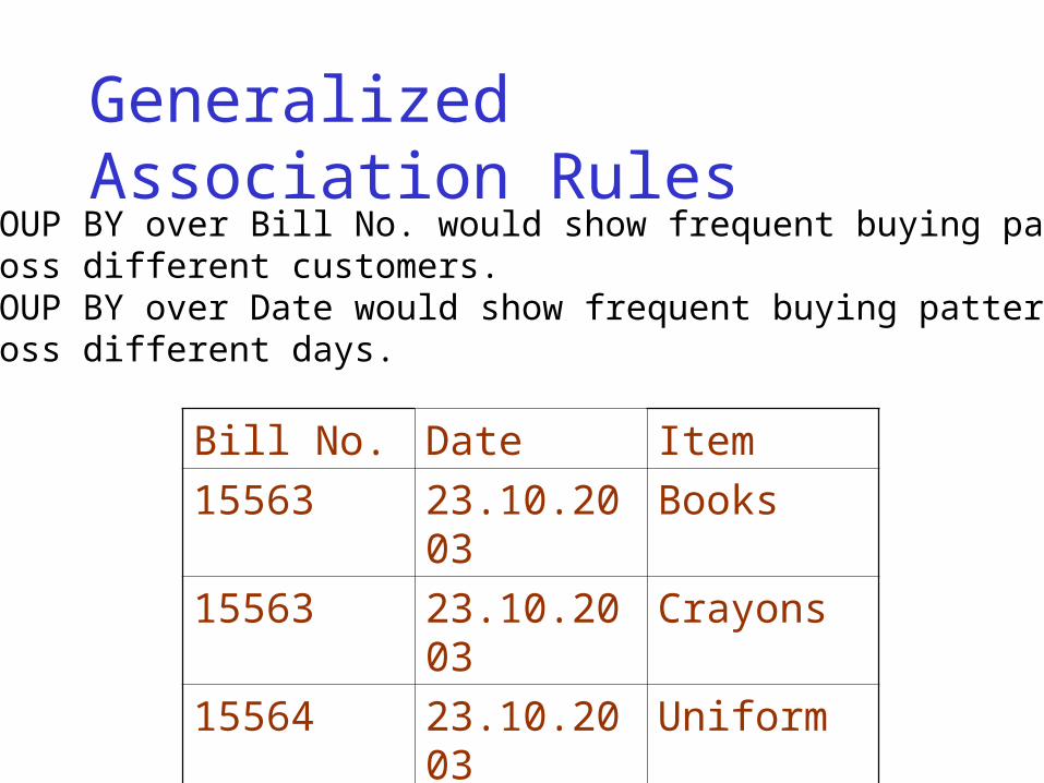
Generalized Association Rules
A GROUP BY over Bill No. would show frequent buying patterns across different customers. A GROUP BY over Date would show frequent buying patterns across different days.
Bill No. Date Item
15563 23.10.2003
Books
15563 23.10.2003
Crayons
15564 23.10.2003
Uniform
15564 23.10.2003
Crayons

Classification and ClusteringGiven a set of data elements:
Classification maps each data element to one of a set of pre-determined classes based on the difference among data elements belonging to different classes
Clustering groups data elements into different groups based on the similarity between elements within a single group

Classification TechniquesDecision Tree Identification
Outlook Temp Play?
Sunny 30 Yes
Overcast 15 No
Sunny 16 Yes
Cloudy 27 Yes
Overcast 25 Yes
Overcast 17 No
Cloudy 17 No
Cloudy 35 Yes
Classification problem
Weather Play(Yes,No)

Classification Techniques
Hunt’s method for decision tree identification:
Given N element types and m decision classes: 1. For i 1 to N do
1. Add element i to the i-1 element item-sets from the previous iteration
2. Identify the set of decision classes for each item-set3. If an item-set has only one decision class, then that
item-set is done, remove that item-set from subsequent iterations
2. done

Classification TechniquesDecision Tree Identification Example
Outlook Temp Play?
Sunny Warm Yes
Overcast Chilly No
Sunny Chilly Yes
Cloudy Pleasant
Yes
Overcast Pleasant
Yes
Overcast Chilly No
Cloudy Chilly No
Cloudy Warm Yes
Sunny
Cloudy
Overcast
Yes
Yes/No
Yes/No

Classification TechniquesDecision Tree Identification Example
Outlook Temp Play?
Sunny Warm Yes
Overcast Chilly No
Sunny Chilly Yes
Cloudy Pleasant
Yes
Overcast Pleasant
Yes
Overcast Chilly No
Cloudy Chilly No
Cloudy Warm Yes
Sunny
Cloudy
Overcast
Yes
Yes/No
Yes/No

Classification TechniquesDecision Tree Identification Example
Outlook Temp Play?
Sunny Warm Yes
Overcast Chilly No
Sunny Chilly Yes
Cloudy Pleasant
Yes
Overcast Pleasant
Yes
Overcast Chilly No
Cloudy Chilly No
Cloudy Warm Yes
CloudyWarm
Yes
CloudyChilly
No
CloudyPleasant
Yes

Classification TechniquesDecision Tree Identification Example
Outlook Temp Play?
Sunny Warm Yes
Overcast Chilly No
Sunny Chilly Yes
Cloudy Pleasant
Yes
Overcast Pleasant
Yes
Overcast Chilly No
Cloudy Chilly No
Cloudy Warm Yes
OvercastWarm
OvercastChilly
No
OvercastPleasant
Yes

Classification TechniquesDecision Tree Identification Example
Yes/No
Yes/No Yes Yes/No
SunnyCloudy Overcast
Yes No YesNo
Yes
WarmChilly
Pleasant Chilly
Pleasant

Classification TechniquesDecision Tree Identification Example
• Top down technique for decision tree identification
• Decision tree created is sensitive to the order in which items are considered
• If an N-item-set does not result in a clear decision, classification classes have to be modeled by rough sets.

Other Classification AlgorithmsQuinlan’s depth-first strategy builds the decision tree in a depth-first fashion, by considering all possible tests that give a decision and selecting the test that gives the best information gain. It hence eliminates tests that are inconclusive.
SLIQ (Supervised Learning in Quest) developed in the QUEST project of IBM uses a top-down breadth-first strategy to build a decision tree. At each level in the tree, an entropy value of each node is calculated and nodes having the lowest entropy values selected and expanded.

Clustering TechniquesClustering partitions the data set into clusters or equivalence classes.
Similarity among members of a class more than similarity among members across classes.
Similarity measures: Euclidian distance or other application specific measures.

Euclidian Distance for Tables
Warm Pleasant Chilly
Sunny
Cloudy
Overcast
Play
Don’t Play
(Cloudy,Pleasant,Play)
(Overcast,Chilly,Don’t Play)

Clustering TechniquesGeneral Strategy:
1. Draw a graph connecting items which are close to one another with edges.
2. Partition the graph into maximally connected subcomponents. 1. Construct an MST for the graph2. Merge items that are connected by the minimum
weight of the MST into a cluster

Clustering TechniquesClustering types:
Hierarchical clustering: Clusters are formed at different levels by merging clusters at a lower level
Partitional clustering: Clusters are formed at only one level

Clustering TechniquesNearest Neighbour Clustering Algorithm:
Given n elements x1, x2, … xn, and threshold t, . 1. j 1, k 1, Clusters = {} 2. Repeat
1. Find the nearest neighbour of xj 2. Let the nearest neighbour be in cluster m 3. If distance to nearest neighbour > t, then create a new
cluster and k k+1; else assign xj to cluster m 4. j j+1
3. until j > n

Clustering TechniquesIterative partitional clustering:
Given n elements x1, x2, … xn, and k clusters, each with a center.
1. Assign each element to its closest cluster center 2. After all assignments have been made, compute the
cluster centroids for each of the cluster 3. Repeat the above two steps with the new centroids until
the algorithm converges

Mining Sequence DataCharacteristics of Sequence Data:
• Collection of data elements which are ordered sequences
• In a sequence, each item has an index associated with it
• A k-sequence is a sequence of length k. Support for sequence j is the number of m-sequences (m>=j) which contain j as a sequence
• Sequence data: transaction logs, DNA sequences, patient ailment history, …

Mining Sequence DataSome Definitions:
• A sequence is a list of itemsets of finite length. • Example:
• {pen,pencil,ink}{pencil,ink}{ink,eraser}{ruler,pencil}• … the purchases of a single customer over time…
• The order of items within an itemset does not matter; but the order of itemsets matter • A subsequence is a sequence with some itemsets deleted

Mining Sequence DataSome Definitions:
• A sequence S’ = {a1, a2, …, am} is said to be contained within another sequence S, if S contains a subsequence {b1, b2, … bm} such that a1 b1, a2 b2, …, am bm.
• Hence, {pen}{pencil}{ruler,pencil} is contained in {pen,pencil,ink}{pencil,ink}{ink,eraser}{ruler,pencil}

Mining Sequence DataApriori Algorithm for Sequences:
1. L1 Set of all interesting 1-sequences 2. k 13. while Lk is not empty do
1. Generate all candidate k+1 sequences 2. Lk+1 Set of all interesting k+1-sequences
4. done
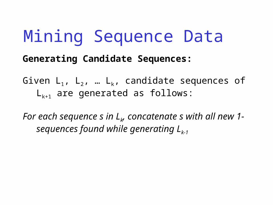
Mining Sequence DataGenerating Candidate Sequences:
Given L1, L2, … Lk, candidate sequences of Lk+1 are generated as follows:
For each sequence s in Lk, concatenate s with all new 1-sequences found while generating Lk-1

Mining Sequence DataExample: minsup = 0.5 a b c d e Interesting 1-sequences: b d a e a a e b d b b e d e a b d a e a a a a b a a a Candidate 2-sequences c b d b aa, ab, ad, ae a b b a b ba, bb, bd, be a b d e da, db, dd, de ea, eb, ed, ee

Mining Sequence DataExample: minsup = 0.5 a b c d e Interesting 2-sequences: b d a e ab, bd a e b d b e Candidate 2-sequences e a b d a aba, abb, abd, abe, a a a a aab, bab, dab, eab, b a a a bda, bdb, bdd, bde, c b d b bbd, dbd, ebd. a b b a b a b d e Interesting 3-sequences = {}

Mining Sequence DataLanguage Inference:
Given a set of sequences, consider each sequence as the behavioural trace of a machine, and infer the machine that can display the given sequence as behavior.
aabb ababcac abbac
…
Input set of sequences Output state machine

Mining Sequence Data
• Inferring the syntax of a language given its sentences
• Applications: discerning behavioural patterns, emergent properties discovery, collaboration modeling, …
• State machine discovery is the reverse of state machine construction
• Discovery is “maximalist” in nature…

Mining Sequence Data“Maximal” nature of language inference:
abc aabc aabbc abbc
a,b,c
a bc
a
b
c
b
c
bc
“Most general” state machine
“Most specific” state machine

Mining Sequence Data“Shortest-run Generalization” (Srinivasa and Spiliopoulou 2000)
Given a set of n sequences: 1. Create a state machine for the first sequence 2. for j 2 to n do
1. Create a state machine for the jth sequence 2. Merge this sequence into the earlier sequence as follows:
1. Merge all halt states in the new state machine to the halt state in the existing state machine
2. If two or more paths to the halt state share the same suffix, merge the suffixes together into a single path
3. Done

Mining Sequence Data“Shortest-run Generalization” (Srinivasa and Spiliopoulou 2000)
aabcb
aac
aabc
a a b c b
a a b c bc
a a b c b
c
a a c bb

Mining Streaming DataCharacteristics of streaming data:
• Large data sequence
• No storage
• Often an infinite sequence
• Examples: Stock market quotes, streaming audio/video, network traffic

Mining Streaming DataRunning mean:
Let n = number of items read so far,
avg = running average calculated so far,
On reading the next number num:
avg (n*avg+num) / (n+1) n n+1

Mining Streaming DataRunning variance:
var = (num-avg)2
= num2 - 2*num*avg + avg2
Let A = num2 of all numbers read so far B = 2*num*avg of all numbers read so far C = avg2 of all numbers read so far avg = average of numbers read so far n = number of numbers read so far

Mining Streaming DataRunning variance:
On reading next number num:
avg (avg*n + num) / (n+1) n n+1
A A + num2
B B + 2*avg*num C C + avg2
var = A + B + C

Mining Streaming Data-Consistency: (Srinivasa and Spiliopoulou, CoopIS 1999)
Let streaming data be in the form of “frames” where each frame comprises of one or more data elements.
Support for data element k within a frame is defined as (#occurrences of k)/(#elements in frame)
-Consistency for data element k is the “sustained” support for k over all frames read so far, with a “leakage” of (1- )

Mining Streaming Data-Consistency: (Srinivasa and Spiliopoulou, CoopIS 1999)
*sup(k)
(1-)
levelt(k) = (1-)*levelt-1(k) + *sup(k)

Data Warehousing
• A platform for online analytical processing (OLAP) • Warehouses collect transactional data from several
transactional databases and organize them in a fashion amenable to analysis
• Also called “data marts”• A critical component of the decision support system
(DSS) of enterprises• Some typical DW queries:
– Which item sells best in each region that has retail outlets
– Which advertising strategy is best for South India? – Which (age_group/occupation) in South India likes fast
food, and which (age_group/occupation) likes to cook?

Data Warehousing
Order Processing
Inventory
Sales
Data Cleaning
DataWarehouse
(OLAP)
OLTP

OLTP vs OLAP
Transactional Data (OLTP)
Analysis Data (OLAP)
Small or medium size databases
Very large databases
Transient data Archival data
Frequent insertions and updates
Infrequent updates
Small query shadow Very large query shadow
Normalization important to handle updates
De-normalization important to handle queries

Data Cleaning
• Performs logical transformation of transactional data to suit the data warehouse
• Model of operations model of enterprise
• Usually a semi-automatic process

Data Cleaning
OrdersOrder_id
PriceCust_id
InventoryProd_id
PricePrice_chng
SalesCust_id
Cust_profTot_sales
Data Warehouse
CustomersProductsOrdersInventoryPriceTime

Multi-dimensional Data Model
Time
Jan’01 Jun’01 Jan’02 Jun’02
Pric
e
Customers Pro
duct
s
Ord
ers

Some MDBMS Operations
• Roll-up– Add dimensions
• Drill-down– Collapse dimensions
• Vector-distance operations (ex: clustering)
• Vector space browsing

Star Schema
Fact tableDimTbl_1
DimTbl_1
DimTbl_1
DimTbl_1

WWW Based References
• http://www.kdnuggets.com/• http://www.megaputer.com/• http://www.almaden.ibm.com/cs/quest/index.html • http://fas.sfu.ca/cs/research/groups/DB/sections/
publication/kdd/kdd.html • http://www.cs.su.oz.au/~thierry/ckdd.html • http://www.dwinfocenter.org/ • http://datawarehouse.itoolbox.com/ • http://www.knowledgestorm.com/ • http://www.bitpipe.com/ • http://www.dw-institute.com/ • http://www.datawarehousing.com/

References• Agrawal, R. Srikant: ``Fast Algorithms for Mining Association
Rules'', Proc. of the 20th Int'l Conference on Very Large Databases, Santiago, Chile, Sept. 1994.
• R. Agrawal, R. Srikant, ``Mining Sequential Patterns'', Proc. of the Int'l Conference on Data Engineering (ICDE), Taipei, Taiwan, March 1995.
• R. Agrawal, A. Arning, T. Bollinger, M. Mehta, J. Shafer, R. Srikant: "The Quest Data Mining System", Proc. of the 2nd Int'l Conference on Knowledge Discovery in Databases and Data Mining, Portland, Oregon, August, 1996.
• Surajit Chaudhuri, Umesh Dayal. An Overview of Data Warehousing and OLAP Technology. ACM SIGMOD Record. 26(1), March 1997.
• Jennifer Widom. Research Problems in Data Warehousing. Proc. of Int’l Conf. On Information and Knowledge Management, 1995.

References• A. Shoshani. OLAP and Statistical Databases:
Similarities and Differences. Proc. of ACM PODS 1997. • Panos Vassiliadis, Timos Sellis. A Survey on Logical
Models for OLAP Databases. ACM SIGMOD Record• M. Gyssens, Laks VS Lakshmanan. A Foundation for
Multi-Dimensional Databases. Proc of VLDB 1997, Athens, Greece.
• Srinath Srinivasa, Myra Spiliopoulou. Modeling Interactions Based on Consistent Patterns. Proc. of CoopIS 1999, Edinburg, UK.
• Srinath Srinivasa, Myra Spiliopoulou. Discerning Behavioral Patterns By Mining Transaction Logs. Proc. of ACM SAC 2000, Como, Italy.