data mining - computer science | academics | wpiweb.cs.wpi.edu/~cs4445/b12/lecturenotes/weka... ·...
TRANSCRIPT

Data MiningPractical Machine Learning Tools and Techniques
Slides for Chapter 6 of Data Mining by I. H. Witten and E. Frank

2Data Mining: Practical Machine Learning Tools and Techniques (Chapter 6)
Implementation:Real machine learning schemes
● Decision trees♦ From ID3 to C4.5 (pruning, numeric attributes, ...)
● Classification rules♦ From PRISM to RIPPER and PART (pruning, numeric data, ...)
● Extending linear models♦ Support vector machines and neural networks
● Instancebased learning♦ Pruning examples, generalized exemplars, distance functions
● Numeric prediction♦ Regression/model trees, locally weighted regression
● Clustering: hierarchical, incremental, probabilistic♦ Hierarchical, incremental, probabilistic
● Bayesian networks♦ Learning and prediction, fast data structures for learning

3Data Mining: Practical Machine Learning Tools and Techniques (Chapter 6)
Industrialstrength algorithms
● For an algorithm to be useful in a wide range of realworld applications it must:
♦ Permit numeric attributes♦ Allow missing values♦ Be robust in the presence of noise♦ Be able to approximate arbitrary concept
descriptions (at least in principle) ● Basic schemes need to be extended to fulfill
these requirements
4Data Mining: Practical Machine Learning Tools and Techniques (Chapter 6)
Decision trees
● Extending ID3:● to permit numeric attributes: straightforward● to deal sensibly with missing values: trickier● stability for noisy data:
requires pruning mechanism● End result: C4.5 (Quinlan)
● Bestknown and (probably) most widelyused learning algorithm
● Commercial successor: C5.0

5Data Mining: Practical Machine Learning Tools and Techniques (Chapter 6)
Numeric attributes
● Standard method: binary splits♦ E.g. temp < 45
● Unlike nominal attributes,every attribute has many possible split points
● Solution is straightforward extension: ♦ Evaluate info gain (or other measure)
for every possible split point of attribute♦ Choose “best” split point♦ Info gain for best split point is info gain for attribute
● Computationally more demanding
6Data Mining: Practical Machine Learning Tools and Techniques (Chapter 6)
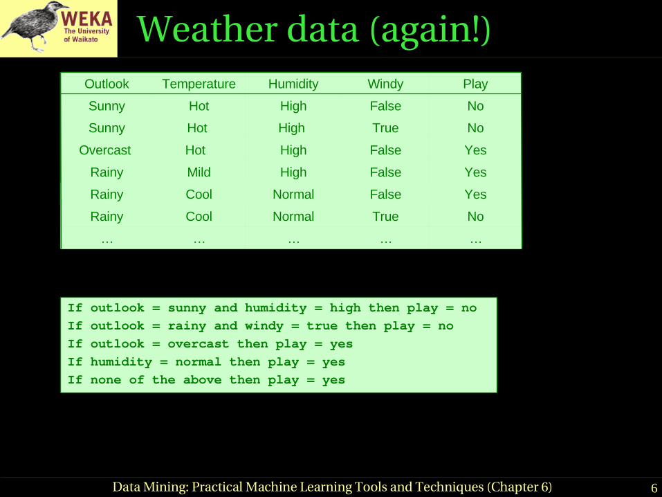
Weather data (again!)
If outlook = sunny and humidity = high then play = no
If outlook = rainy and windy = true then play = no
If outlook = overcast then play = yes
If humidity = normal then play = yes
If none of the above then play = yes
……………
YesFalseNormalMildRainy
YesFalseHighHot Overcast
NoTrueHigh Hot Sunny
NoFalseHighHotSunny
PlayWindyHumidityTemperatureOutlook
……………
YesFalseNormalMildRainy
YesFalseHighHot Overcast
NoTrueHigh Hot Sunny
NoFalseHighHotSunny
PlayWindyHumidityTemperatureOutlook
……………
YesFalseHighMildRainy
YesFalseHighHot Overcast
NoTrueHigh Hot Sunny
NoFalseHighHotSunny
PlayWindyHumidityTemperatureOutlook
…………… …………… NoTrueNormalCoolRainy
…………… …………… ……………
…………… …………… YesFalseNormalCoolRainy
7Data Mining: Practical Machine Learning Tools and Techniques (Chapter 6)
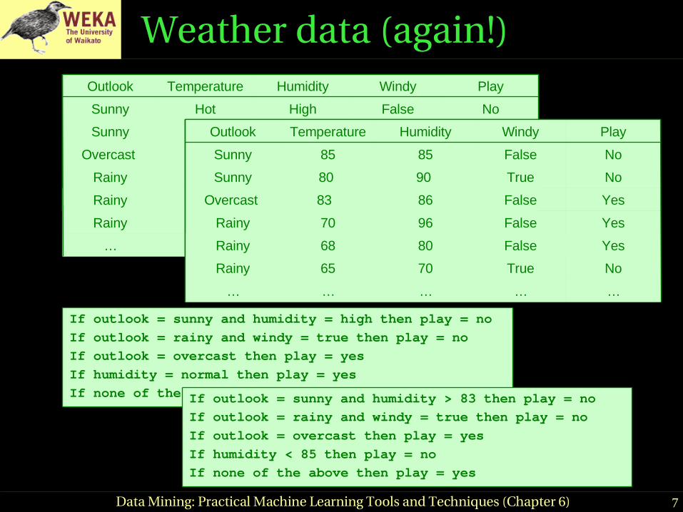
Weather data (again!)
If outlook = sunny and humidity = high then play = no
If outlook = rainy and windy = true then play = no
If outlook = overcast then play = yes
If humidity = normal then play = yes
If none of the above then play = yesIf outlook = sunny and humidity > 83 then play = no
If outlook = rainy and windy = true then play = no
If outlook = overcast then play = yes
If humidity < 85 then play = no
If none of the above then play = yes
……………
YesFalseNormalMildRainy
YesFalseHighHot Overcast
NoTrueHigh Hot Sunny
NoFalseHighHotSunny
PlayWindyHumidityTemperatureOutlook
……………
YesFalseNormalMildRainy
YesFalseHighHot Overcast
NoTrueHigh Hot Sunny
NoFalseHighHotSunny
PlayWindyHumidityTemperatureOutlook
……………
YesFalseHighMildRainy
YesFalseHighHot Overcast
NoTrueHigh Hot Sunny
NoFalseHighHotSunny
PlayWindyHumidityTemperatureOutlook
…………… …………… NoTrueNormalCoolRainy
…………… …………… ……………
…………… …………… YesFalseNormalCoolRainy
……………
YesFalseNormalMildRainy
YesFalseHighHot Overcast
NoTrueHigh Hot Sunny
NoFalseHighHotSunny
PlayWindyHumidityTemperatureOutlook
……………
YesFalseNormalMildRainy
YesFalseHighHot Overcast
NoTrueHigh Hot Sunny
NoFalseHighHotSunny
PlayWindyHumidityTemperatureOutlook
……………
YesFalse9670Rainy
YesFalse8683 Overcast
NoTrue90 80 Sunny
NoFalse8585Sunny
PlayWindyHumidityTemperatureOutlook
…………… …………… NoTrue7065Rainy
…………… …………… ……………
…………… …………… YesFalse8068Rainy

8Data Mining: Practical Machine Learning Tools and Techniques (Chapter 6)
Example
● Split on temperature attribute:
♦ E.g. temperature < 71.5: yes/4, no/2temperature ≥ 71.5: yes/5, no/3
♦ Info([4,2],[5,3])= 6/14 info([4,2]) + 8/14 info([5,3]) = 0.939 bits
● Place split points halfway between values● Can evaluate all split points in one pass!
64 65 68 69 70 71 72 72 75 75 80 81 83 85Yes No Yes Yes Yes No No Yes Yes Yes No Yes Yes No

9Data Mining: Practical Machine Learning Tools and Techniques (Chapter 6)
Can avoid repeated sorting
● Sort instances by the values of the numeric attribute♦ Time complexity for sorting: O (n log n)
● Does this have to be repeated at each node of the tree?
● No! Sort order for children can be derived from sort order for parent
♦ Time complexity of derivation: O (n)♦ Drawback: need to create and store an array of sorted
indices for each numeric attribute
10Data Mining: Practical Machine Learning Tools and Techniques (Chapter 6)
Binary vs multiway splits
● Splitting (multiway) on a nominal attribute exhausts all information in that attribute
♦ Nominal attribute is tested (at most) once on any path in the tree
● Not so for binary splits on numeric attributes!♦ Numeric attribute may be tested several times along a
path in the tree● Disadvantage: tree is hard to read● Remedy:
♦ prediscretize numeric attributes, or♦ use multiway splits instead of binary ones

11Data Mining: Practical Machine Learning Tools and Techniques (Chapter 6)
Computing multiway splits
● Simple and efficient way of generating multiway splits: greedy algorithm
● Dynamic programming can find optimum multiway split in O (n2) time
♦ imp (k, i, j ) is the impurity of the best split of values xi … xj into k subintervals
♦ imp (k, 1, i ) = min0<j <i imp (k–1, 1, j ) + imp (1, j+1, i )
♦ imp (k, 1, N ) gives us the best kway split● In practice, greedy algorithm works as well
12Data Mining: Practical Machine Learning Tools and Techniques (Chapter 6)
Missing values
● Split instances with missing values into pieces♦ A piece going down a branch receives a weight
proportional to the popularity of the branch♦ weights sum to 1
● Info gain works with fractional instances♦ use sums of weights instead of counts
● During classification, split the instance into pieces in the same way
♦ Merge probability distribution using weights
13Data Mining: Practical Machine Learning Tools and Techniques (Chapter 6)
Pruning
● Prevent overfitting to noise in the data● “Prune” the decision tree● Two strategies:
● Postpruningtake a fullygrown decision tree and discard unreliable parts
● Prepruningstop growing a branch when information becomes unreliable
● Postpruning preferred in practice—prepruning can “stop early”
14Data Mining: Practical Machine Learning Tools and Techniques (Chapter 6)
Prepruning
● Based on statistical significance test♦ Stop growing the tree when there is no statistically
significant association between any attribute and the class at a particular node
● Most popular test: chisquared test● ID3 used chisquared test in addition to
information gain♦ Only statistically significant attributes were allowed to
be selected by information gain procedure

15Data Mining: Practical Machine Learning Tools and Techniques (Chapter 6)
Early stopping
● Prepruning may stop the growthprocess prematurely: early stopping
● Classic example: XOR/Parityproblem♦ No individual attribute exhibits any significant
association to the class♦ Structure is only visible in fully expanded tree♦ Prepruning won’t expand the root node
● But: XORtype problems rare in practice● And: prepruning faster than postpruning
0001
1102
1
1
a
014
103
cl assb
16Data Mining: Practical Machine Learning Tools and Techniques (Chapter 6)
Postpruning
● First, build full tree● Then, prune it
● Fullygrown tree shows all attribute interactions ● Problem: some subtrees might be due to
chance effects● Two pruning operations:
● Subtree replacement● Subtree raising
● Possible strategies:● error estimation● significance testing● MDL principle

17Data Mining: Practical Machine Learning Tools and Techniques (Chapter 6)
Subtree replacement
● Bottomup● Consider replacing a tree only
after considering all its subtrees
18Data Mining: Practical Machine Learning Tools and Techniques (Chapter 6)
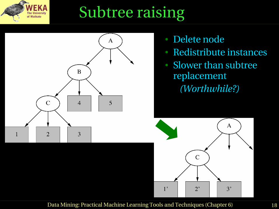
Subtree raising
● Delete node● Redistribute instances● Slower than subtree
replacement(Worthwhile?)
19Data Mining: Practical Machine Learning Tools and Techniques (Chapter 6)
Estimating error rates
● Prune only if it does not increase the estimated error● Error on the training data is NOT a useful estimator
(would result in almost no pruning)● Use holdout set for pruning
(“reducederror pruning”)● C4.5’s method
♦ Derive confidence interval from training data♦ Use a heuristic limit, derived from this, for pruning♦ Standard Bernoulliprocessbased method♦ Shaky statistical assumptions (based on training data)
20Data Mining: Practical Machine Learning Tools and Techniques (Chapter 6)
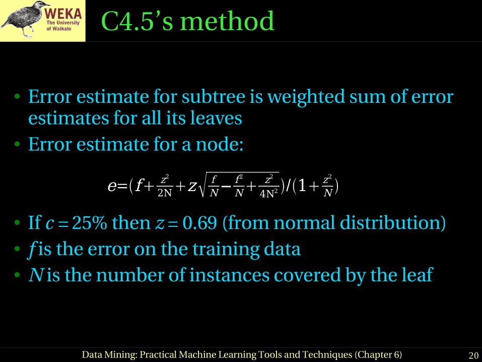
C4.5’s method
● Error estimate for subtree is weighted sum of error estimates for all its leaves
● Error estimate for a node:
● If c = 25% then z = 0.69 (from normal distribution)● f is the error on the training data● N is the number of instances covered by the leaf
e=f z2
2Nz fN−
f2
Nz2
4N2 /1 z2
N

21Data Mining: Practical Machine Learning Tools and Techniques (Chapter 6)
Example
f=0.33 e=0.47
f=0.5 e=0.72
f=0.33 e=0.47
f = 5/14 e = 0.46e < 0.51so prune!
Combined using ratios 6:2:6 gives 0.51
22Data Mining: Practical Machine Learning Tools and Techniques (Chapter 6)
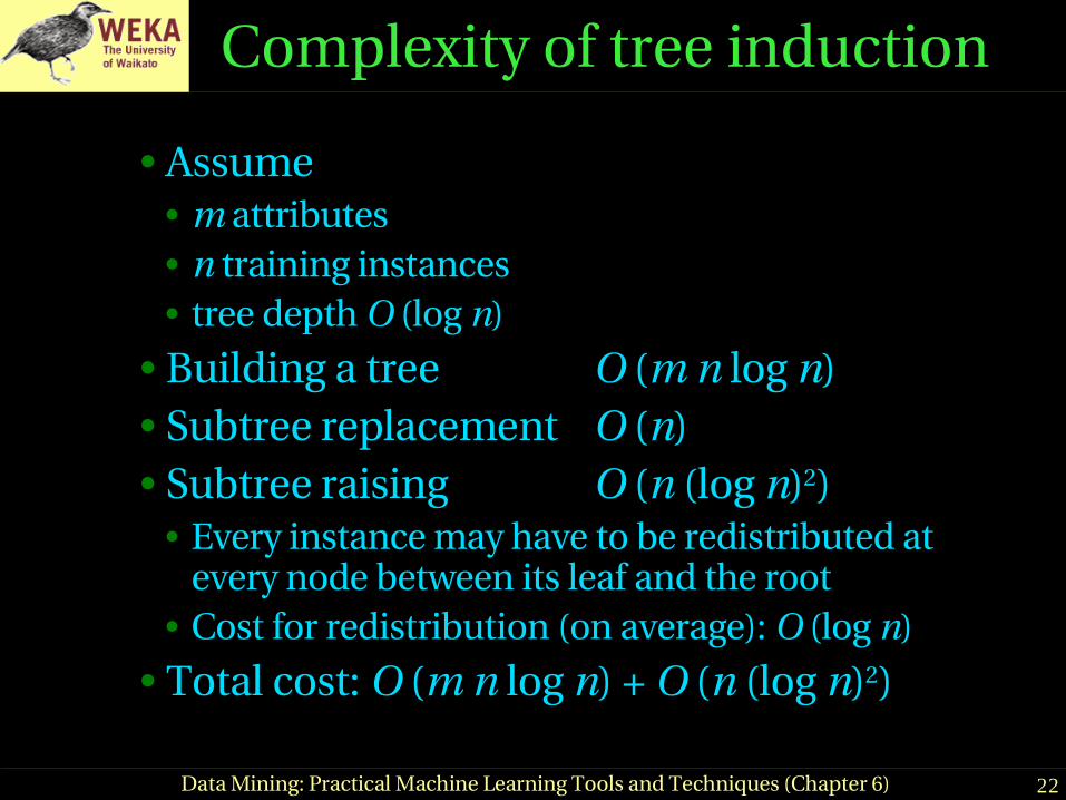
Complexity of tree induction
● Assume● m attributes● n training instances● tree depth O (log n)
● Building a tree O (m n log n)● Subtree replacement O (n)● Subtree raising O (n (log n)2)
● Every instance may have to be redistributed at every node between its leaf and the root
● Cost for redistribution (on average): O (log n)● Total cost: O (m n log n) + O (n (log n)2)

23Data Mining: Practical Machine Learning Tools and Techniques (Chapter 6)
From trees to rules● Simple way: one rule for each leaf● C4.5rules: greedily prune conditions from each
rule if this reduces its estimated error● Can produce duplicate rules● Check for this at the end
● Then● look at each class in turn● consider the rules for that class● find a “good” subset (guided by MDL)
● Then rank the subsets to avoid conflicts● Finally, remove rules (greedily) if this decreases
error on the training data
24Data Mining: Practical Machine Learning Tools and Techniques (Chapter 6)
C4.5: choices and options
● C4.5rules slow for large and noisy datasets● Commercial version C5.0rules uses a
different technique♦ Much faster and a bit more accurate
● C4.5 has two parameters♦ Confidence value (default 25%):
lower values incur heavier pruning♦ Minimum number of instances in the two most
popular branches (default 2)

25Data Mining: Practical Machine Learning Tools and Techniques (Chapter 6)
Discussion
● The most extensively studied method of machine learning used in data mining
● Different criteria for attribute/test selection rarely make a large difference
● Different pruning methods mainly change the size of the resulting pruned tree
● C4.5 builds univariate decision trees● Some TDITDT systems can build
multivariate trees (e.g. CART)
TDIDT: TopDown Induction of Decision Trees

26Data Mining: Practical Machine Learning Tools and Techniques (Chapter 6)
Classification rules
● Common procedure: separateandconquer ● Differences:
♦ Search method (e.g. greedy, beam search, ...)♦ Test selection criteria (e.g. accuracy, ...)♦ Pruning method (e.g. MDL, holdout set, ...)♦ Stopping criterion (e.g. minimum accuracy)♦ Postprocessing step
● Also: Decision listvs. one rule set for each class
27Data Mining: Practical Machine Learning Tools and Techniques (Chapter 6)
Test selection criteria● Basic covering algorithm:
♦ keep adding conditions to a rule to improve its accuracy♦ Add the condition that improves accuracy the most
● Measure 1: p/t♦ t total instances covered by rule
p number of these that are positive♦ Produce rules that don’t cover negative instances,
as quickly as possible♦ May produce rules with very small coverage
—special cases or noise?● Measure 2: Information gain p (log(p/t) – log(P/T))
♦ P and T the positive and total numbers before the new condition was added
♦ Information gain emphasizes positive rather than negative instances● These interact with the pruning mechanism used
28Data Mining: Practical Machine Learning Tools and Techniques (Chapter 6)
Missing values, numeric attributes
● Common treatment of missing values:for any test, they fail
♦ Algorithm must either● use other tests to separate out positive instances● leave them uncovered until later in the process
● In some cases it’s better to treat “missing” as a separate value
● Numeric attributes are treated just like they are in decision trees

29Data Mining: Practical Machine Learning Tools and Techniques (Chapter 6)
Pruning rules
● Two main strategies:♦ Incremental pruning♦ Global pruning
● Other difference: pruning criterion♦ Error on holdout set (reducederror pruning)♦ Statistical significance♦ MDL principle
● Also: postpruning vs. prepruning
30Data Mining: Practical Machine Learning Tools and Techniques (Chapter 6)
Using a pruning set
● For statistical validity, must evaluate measure on data not used for training:
♦ This requires a growing set and a pruning set● Reducederror pruning :
build full rule set and then prune it● Incremental reducederror pruning :
simplify each rule as soon as it is built♦ Can resplit data after rule has been pruned
● Stratification advantageous
31Data Mining: Practical Machine Learning Tools and Techniques (Chapter 6)
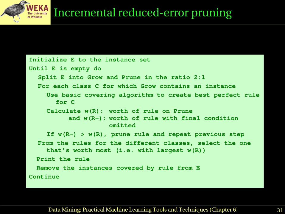
Incremental reducederror pruning
Initialize E to the instance set
Until E is empty do
Split E into Grow and Prune in the ratio 2:1
For each class C for which Grow contains an instance
Use basic covering algorithm to create best perfect rulefor C
Calculate w(R): worth of rule on Prune and w(R-): worth of rule with final condition
omitted
If w(R-) > w(R), prune rule and repeat previous step
From the rules for the different classes, select the onethat’s worth most (i.e. with largest w(R))
Print the rule
Remove the instances covered by rule from E
Continue

32Data Mining: Practical Machine Learning Tools and Techniques (Chapter 6)
Measures used in IREP
● [p + (N – n)] / T ♦ (N is total number of negatives)♦ Counterintuitive:
● p = 2000 and n = 1000 vs. p = 1000 and n = 1● Success rate p / t
♦ Problem: p = 1 and t = 1 vs. p = 1000 and t = 1001
● (p – n) / t♦ Same effect as success rate because it equals 2p/t – 1
● Seems hard to find a simple measure of a rule’s worth that corresponds with intuition

33Data Mining: Practical Machine Learning Tools and Techniques (Chapter 6)
Variations
● Generating rules for classes in order♦ Start with the smallest class♦ Leave the largest class covered by the default rule
● Stopping criterion♦ Stop rule production if accuracy becomes too low
● Rule learner RIPPER:♦ Uses MDLbased stopping criterion♦ Employs postprocessing step to modify rules
guided by MDL criterion

34Data Mining: Practical Machine Learning Tools and Techniques (Chapter 6)
Using global optimization● RIPPER: Repeated Incremental Pruning to Produce Error
Reduction (does global optimization in an efficient way)● Classes are processed in order of increasing size● Initial rule set for each class is generated using IREP● An MDLbased stopping condition is used
♦ DL: bits needs to send examples wrt set of rules, bits needed to send k tests, and bits for k
● Once a rule set has been produced for each class, each rule is reconsidered and two variants are produced
♦ One is an extended version, one is grown from scratch♦ Chooses among three candidates according to DL
● Final cleanup step greedily deletes rules to minimize DL

35Data Mining: Practical Machine Learning Tools and Techniques (Chapter 6)
PART
● Avoids global optimization step used in C4.5rules and RIPPER
● Generates an unrestricted decision list using basic separateandconquer procedure
● Builds a partial decision tree to obtain a rule♦ A rule is only pruned if all its implications are known♦ Prevents hasty generalization
● Uses C4.5’s procedures to build a tree

36Data Mining: Practical Machine Learning Tools and Techniques (Chapter 6)
Building a partial tree
Expand-subset (S):
Choose test T and use it to split set of examplesinto subsets
Sort subsets into increasing order of averageentropy
while there is a subset X not yet been expandedAND all subsets expanded so far are leaves
expand-subset(X)
ifall subsets expanded are leavesAND estimated error for subtree
≥ estimated error for node undo expansion into subsets and make node a leaf

37Data Mining: Practical Machine Learning Tools and Techniques (Chapter 6)
Example
38Data Mining: Practical Machine Learning Tools and Techniques (Chapter 6)
Notes on PART
● Make leaf with maximum coverage into a rule● Treat missing values just as C4.5 does
♦ I.e. split instance into pieces● Time taken to generate a rule:
♦ Worst case: same as for building a pruned tree● Occurs when data is noisy
♦ Best case: same as for building a single rule● Occurs when data is noise free
39Data Mining: Practical Machine Learning Tools and Techniques (Chapter 6)
Rules with exceptions
1.Given: a way of generating a single good rule2.Then it’s easy to generate rules with exceptions3.Select default class for toplevel rule4.Generate a good rule for one of the remaining
classes5.Apply this method recursively to the two subsets
produced by the rule(I.e. instances that are covered/not covered)

40Data Mining: Practical Machine Learning Tools and Techniques (Chapter 6)
Iris data example
Exceptions are represented asDotted paths , a lternatives as solid ones .

41Data Mining: Practical Machine Learning Tools and Techniques (Chapter 6)
Extending linear classification
● Linear classifiers can’t model nonlinear class boundaries
● Simple trick:♦ Map attributes into new space consisting of
combinations of attribute values♦ E.g.: all products of n factors that can be
constructed from the attributes● Example with two attributes and n = 3:
x=w1a13w2a1
2a2w3a1a22w4a2
3

42Data Mining: Practical Machine Learning Tools and Techniques (Chapter 6)
Problems with this approach
● 1st problem: speed♦ 10 attributes, and n = 5 ⇒ >2000 coefficients♦ Use linear regression with attribute selection♦ Run time is cubic in number of attributes
● 2nd problem: overfitting♦ Number of coefficients is large relative to the
number of training instances♦ Curse of dimensionality kicks in

43Data Mining: Practical Machine Learning Tools and Techniques (Chapter 6)
Support vector machines
● Support vector machines are algorithms for learning linear classifiers
● Resilient to overfitting because they learn a particular linear decision boundary:
♦ The maximum margin hyperplane● Fast in the nonlinear case
♦ Use a mathematical trick to avoid creating “pseudoattributes”
♦ The nonlinear space is created implicitly

44Data Mining: Practical Machine Learning Tools and Techniques (Chapter 6)
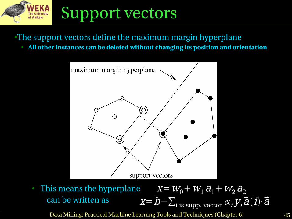
The maximum margin hyperplane
● The instances closest to the maximum margin hyperplane are called support vectors
45Data Mining: Practical Machine Learning Tools and Techniques (Chapter 6)
Support vectors
● This means the hyperplanecan be written as
●The support vectors define the maximum margin hyperplane● All other instances can be deleted without changing its position and orientation
x=w0w1a1w2a2
x=b∑i is supp. vector i yi ai⋅a

46Data Mining: Practical Machine Learning Tools and Techniques (Chapter 6)
Finding support vectors
● Support vector: training instance for which αi > 0● Determine αi and b ?—
A constrained quadratic optimization problem♦ Offtheshelf tools for solving these problems♦ However, specialpurpose algorithms are faster♦ Example: Platt’s sequential minimal optimization
algorithm (implemented in WEKA)● Note: all this assumes separable data!
x=b∑i is supp. vector i yia i⋅a
47Data Mining: Practical Machine Learning Tools and Techniques (Chapter 6)
Nonlinear SVMs
● “Pseudo attributes” represent attribute combinations
● Overfitting not a problem because the maximum margin hyperplane is stable
♦ There are usually few support vectors relative to the size of the training set
● Computation time still an issue♦ Each time the dot product is computed, all the
“pseudo attributes” must be included
48Data Mining: Practical Machine Learning Tools and Techniques (Chapter 6)
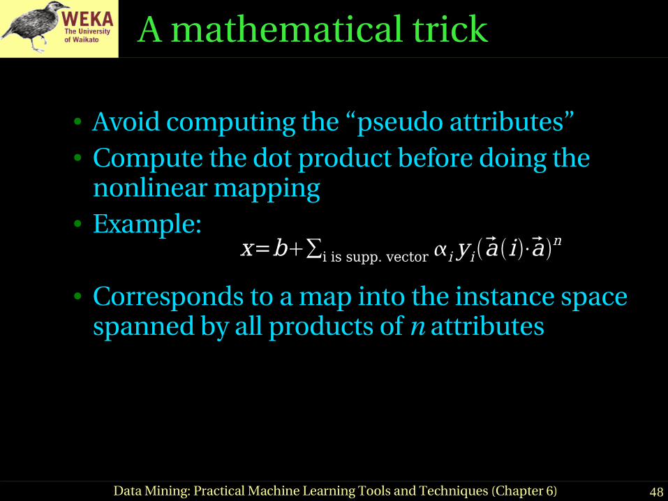
A mathematical trick
● Avoid computing the “pseudo attributes”● Compute the dot product before doing the
nonlinear mapping ● Example:
● Corresponds to a map into the instance space spanned by all products of n attributes
x=b∑i is supp. vector i yi a i⋅an
49Data Mining: Practical Machine Learning Tools and Techniques (Chapter 6)
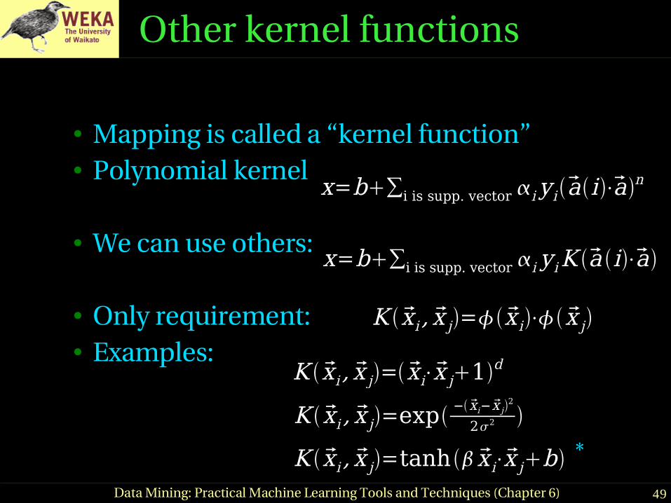
Other kernel functions
● Mapping is called a “kernel function”● Polynomial kernel
● We can use others:
● Only requirement:● Examples:
x=b∑i is supp. vector i yiai⋅an
x=b∑i is supp. vector i yiK a i⋅a
K xi , x j= x i⋅ x j
K xi , x j= xi⋅x j1d
K xi , x j=exp − xi− x j2
22
K xi , x j=tanh x i⋅x jb *

50Data Mining: Practical Machine Learning Tools and Techniques (Chapter 6)
Noise
● Have assumed that the data is separable (in original or transformed space)
● Can apply SVMs to noisy data by introducing a “noise” parameter C
● C bounds the influence of any one training instance on the decision boundary
♦ Corresponding constraint: 0 ≤ αi ≤ C
● Still a quadratic optimization problem● Have to determine C by experimentation
51Data Mining: Practical Machine Learning Tools and Techniques (Chapter 6)
Sparse data
● SVM algorithms speed up dramatically if the data is sparse (i.e. many values are 0)
● Why? Because they compute lots and lots of dot products
● Sparse data ⇒ compute dot products very efficiently● Iterate only over nonzero values
● SVMs can process sparse datasets with 10,000s of attributes

52Data Mining: Practical Machine Learning Tools and Techniques (Chapter 6)
Applications
● Machine vision: e.g face identification● Outperforms alternative approaches (1.5% error)
● Handwritten digit recognition: USPS data● Comparable to best alternative (0.8% error)
● Bioinformatics: e.g. prediction of protein secondary structure
● Text classifiation● Can modify SVM technique for numeric
prediction problems
53Data Mining: Practical Machine Learning Tools and Techniques (Chapter 6)
Support vector regression
● Maximum margin hyperplane only applies to classification
● However, idea of support vectors and kernel functions can be used for regression
● Basic method same as in linear regression: want to minimize error
♦ Difference A: ignore errors smaller than ε and use absolute error instead of squared error
♦ Difference B: simultaneously aim to maximize flatness of function
● Userspecified parameter ε defines “tube”

54Data Mining: Practical Machine Learning Tools and Techniques (Chapter 6)
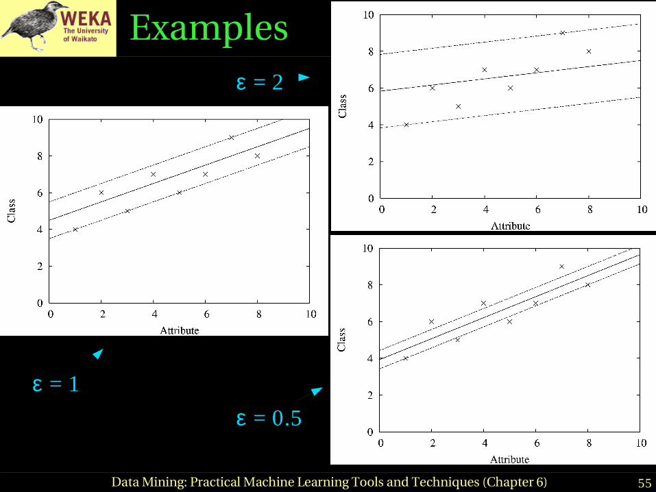
More on SVM regression● If there are tubes that enclose all the training points,
the flattest of them is used♦ Eg.: mean is used if 2ε > range of target values
● Model can be written as:
♦ Support vectors: points on or outside tube♦ Dot product can be replaced by kernel function♦ Note: coefficients α
imay be negative
● No tube that encloses all training points?♦ Requires tradeoff between error and flatness♦ Controlled by upper limit C on absolute value of
coefficients αi
x=b∑i is supp. vector ia i⋅a
55Data Mining: Practical Machine Learning Tools and Techniques (Chapter 6)
Examplesε = 2
ε = 1
ε = 0.5
56Data Mining: Practical Machine Learning Tools and Techniques (Chapter 6)
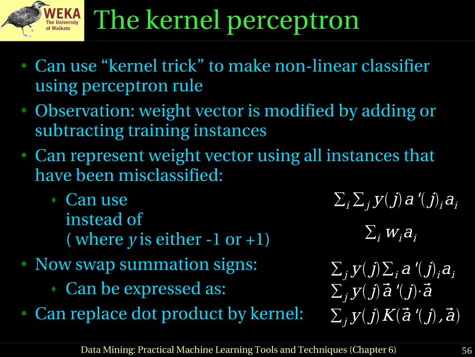
The kernel perceptron
● Can use “kernel trick” to make nonlinear classifier using perceptron rule
● Observation: weight vector is modified by adding or subtracting training instances
● Can represent weight vector using all instances that have been misclassified:
♦ Can use instead of ( where y is either 1 or +1)
● Now swap summation signs:♦ Can be expressed as:
● Can replace dot product by kernel:
∑i wiai
∑i ∑ j y ja' jiai
∑ j y j∑i a' jiai
∑ j y ja' j⋅a∑ j y jK a' j ,a
57Data Mining: Practical Machine Learning Tools and Techniques (Chapter 6)
Comments on kernel perceptron● Finds separating hyperplane in space created by kernel
function (if it exists)♦ But: doesn't find maximummargin hyperplane
● Easy to implement, supports incremental learning● Linear and logistic regression can also be upgraded
using the kernel trick♦ But: solution is not “sparse”: every training instance
contributes to solution● Perceptron can be made more stable by using all weight
vectors encountered during learning, not just last one (voted perceptron)
♦ Weight vectors vote on prediction (vote based on number of successful classifications since inception)
58Data Mining: Practical Machine Learning Tools and Techniques (Chapter 6)
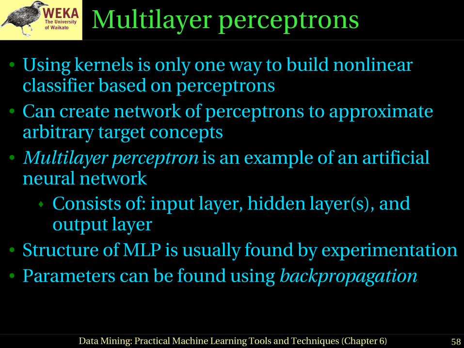
Multilayer perceptrons
● Using kernels is only one way to build nonlinear classifier based on perceptrons
● Can create network of perceptrons to approximate arbitrary target concepts
● Multilayer perceptron is an example of an artificial neural network
♦ Consists of: input layer, hidden layer(s), and output layer
● Structure of MLP is usually found by experimentation● Parameters can be found using backpropagation
59Data Mining: Practical Machine Learning Tools and Techniques (Chapter 6)
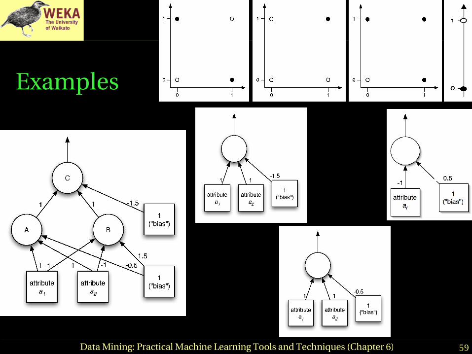
Examples

60Data Mining: Practical Machine Learning Tools and Techniques (Chapter 6)
Backpropagation
● How to learn weights given network structure?♦ Cannot simply use perceptron learning rule because
we have hidden layer(s)♦ Function we are trying to minimize: error♦ Can use a general function minimization technique
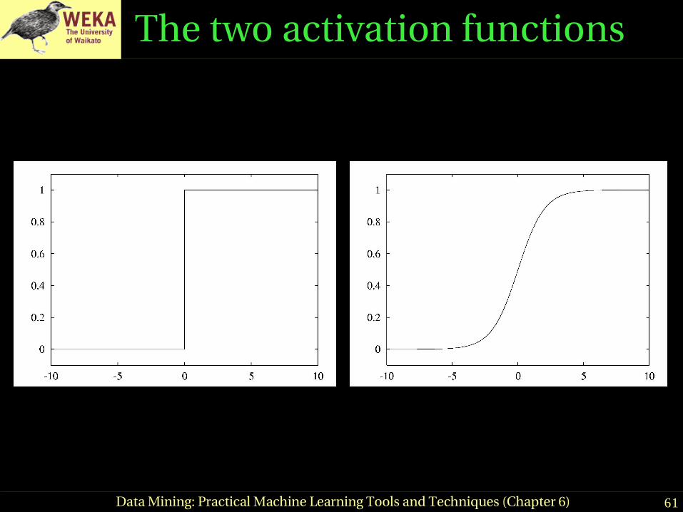
called gradient descent● Need differentiable activation function: use sigmoid
function instead of threshold function
● Need differentiable error function: can't use zeroone loss, but can use squared error
f x = 11exp −x
E= 12 y−f x2
61Data Mining: Practical Machine Learning Tools and Techniques (Chapter 6)
The two activation functions

62Data Mining: Practical Machine Learning Tools and Techniques (Chapter 6)
Gradient descent example
● Function: x2+1● Derivative: 2x● Learning rate: 0.1● Start value: 4
Can only find a local minimum!
63Data Mining: Practical Machine Learning Tools and Techniques (Chapter 6)
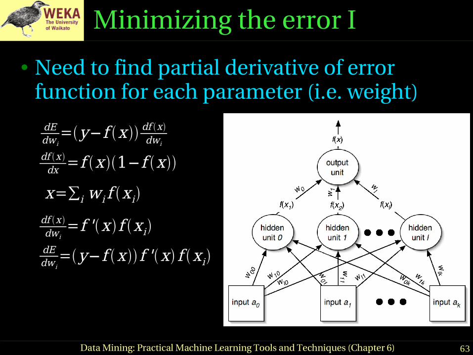
Minimizing the error I
● Need to find partial derivative of error function for each parameter (i.e. weight)
dEdw i
=y−f x df xdwi
df x dx =f x 1−f x
x=∑i wi f xidf x dwi
=f 'x f xidEdw i
=y−f xf 'x f xi

64Data Mining: Practical Machine Learning Tools and Techniques (Chapter 6)
Minimizing the error II
● What about the weights for the connections from the input to the hidden layer?
dEdw ij
= dEdx
dxdwij
=y−f xf 'x dxdw ij
x=∑i wi f xi
dxdw ij
=widf xidwij
dEdw ij
=y−f xf 'xwi f 'xiai
df x i
dw ij=f 'x i
dx i
dwij=f 'xiai

65Data Mining: Practical Machine Learning Tools and Techniques (Chapter 6)
Remarks● Same process works for multiple hidden layers and
multiple output units (eg. for multiple classes)● Can update weights after all training instances have been
processed or incrementally:♦ batch learning vs. stochastic backpropagation♦ Weights are initialized to small random values
● How to avoid overfitting?♦ Early stopping: use validation set to check when to stop♦ Weight decay: add penalty term to error function
● How to speed up learning?♦ Momentum: reuse proportion of old weight change ♦ Use optimization method that employs 2nd derivative

66Data Mining: Practical Machine Learning Tools and Techniques (Chapter 6)
Radial basis function networks
● Another type of feedforward network with two layers (plus the input layer)
● Hidden units represent points in instance space and activation depends on distance
♦ To this end, distance is converted into similarity: Gaussian activation function
● Width may be different for each hidden unit♦ Points of equal activation form hypersphere
(or hyperellipsoid) as opposed to hyperplane● Output layer same as in MLP

67Data Mining: Practical Machine Learning Tools and Techniques (Chapter 6)
Learning RBF networks
● Parameters: centers and widths of the RBFs + weights in output layer
● Can learn two sets of parameters independently and still get accurate models
♦ Eg.: clusters from kmeans can be used to form basis functions
♦ Linear model can be used based on fixed RBFs♦ Makes learning RBFs very efficient
● Disadvantage: no builtin attribute weighting based on relevance
● RBF networks are related to RBF SVMs
68Data Mining: Practical Machine Learning Tools and Techniques (Chapter 6)
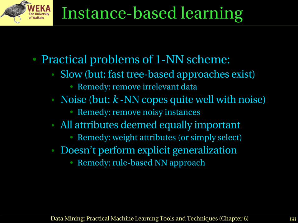
Instancebased learning
● Practical problems of 1NN scheme:♦ Slow (but: fast treebased approaches exist)
● Remedy: remove irrelevant data
♦ Noise (but: k NN copes quite well with noise)● Remedy: remove noisy instances
♦ All attributes deemed equally important● Remedy: weight attributes (or simply select)
♦ Doesn’t perform explicit generalization● Remedy: rulebased NN approach
69Data Mining: Practical Machine Learning Tools and Techniques (Chapter 6)
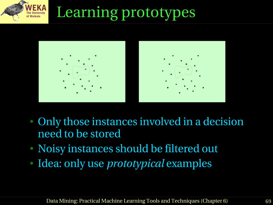
Learning prototypes
● Only those instances involved in a decision need to be stored
● Noisy instances should be filtered out● Idea: only use prototypical examples

70Data Mining: Practical Machine Learning Tools and Techniques (Chapter 6)
Speed up, combat noise
● IB2: save memory, speed up classification♦ Work incrementally♦ Only incorporate misclassified instances♦ Problem: noisy data gets incorporated
● IB3: deal with noise♦ Discard instances that don’t perform well ♦ Compute confidence intervals for
● 1. Each instance’s success rate● 2. Default accuracy of its class
♦ Accept/reject instances● Accept if lower limit of 1 exceeds upper limit of 2● Reject if upper limit of 1 is below lower limit of 2
71Data Mining: Practical Machine Learning Tools and Techniques (Chapter 6)
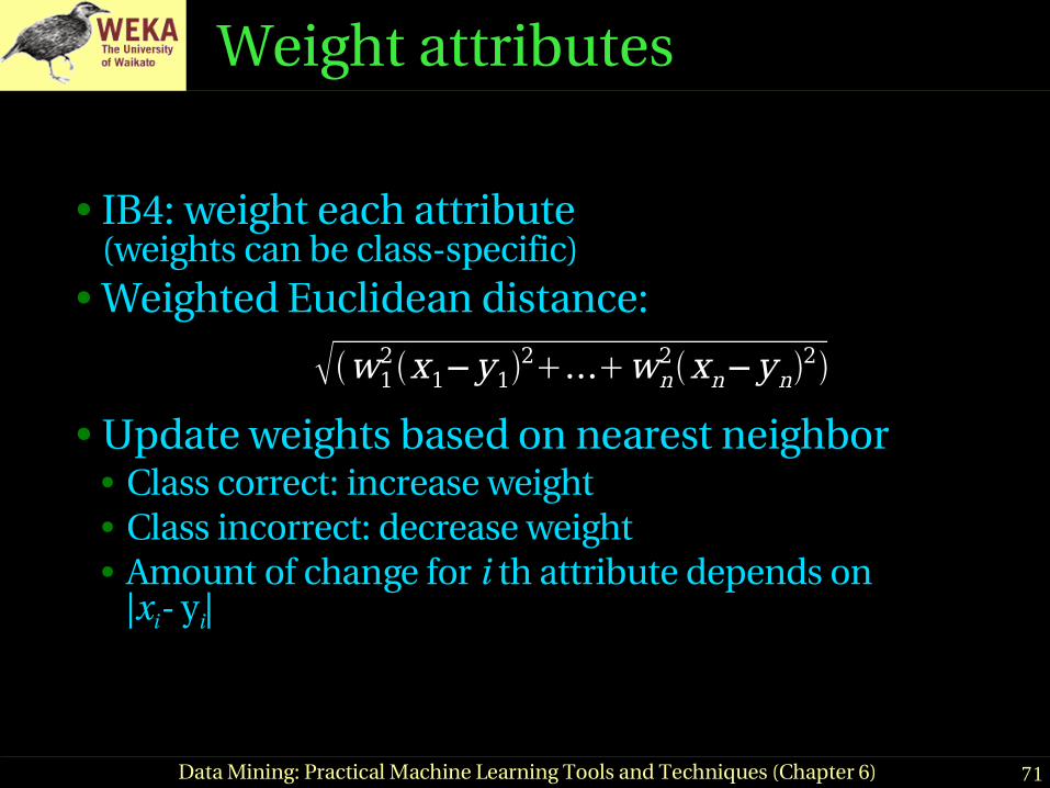
Weight attributes
● IB4: weight each attribute(weights can be classspecific)
● Weighted Euclidean distance:
● Update weights based on nearest neighbor● Class correct: increase weight● Class incorrect: decrease weight● Amount of change for i th attribute depends on
|xi yi|
w12x1−y1
2...wn2xn−yn
2

72Data Mining: Practical Machine Learning Tools and Techniques (Chapter 6)
Rectangular generalizations
● Nearestneighbor rule is used outside rectangles● Rectangles are rules! (But they can be more
conservative than “normal” rules.) ● Nested rectangles are rules with exceptions
73Data Mining: Practical Machine Learning Tools and Techniques (Chapter 6)
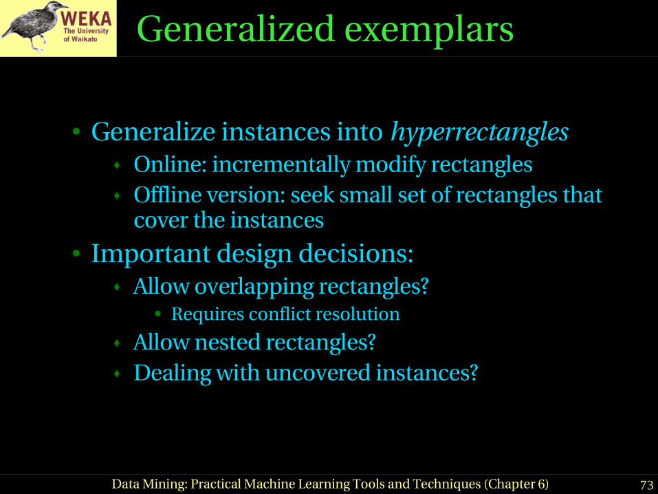
Generalized exemplars
● Generalize instances into hyperrectangles♦ Online: incrementally modify rectangles♦ Offline version: seek small set of rectangles that
cover the instances● Important design decisions:
♦ Allow overlapping rectangles?● Requires conflict resolution
♦ Allow nested rectangles?♦ Dealing with uncovered instances?

74Data Mining: Practical Machine Learning Tools and Techniques (Chapter 6)
Separating generalized exemplars
Class 1
Class2
Separation line

75Data Mining: Practical Machine Learning Tools and Techniques (Chapter 6)
Generalized distance functions
● Given: some transformation operations on attributes
● K*: similarity = probability of transforming instance A into B by chance
● Average over all transformation paths● Weight paths according their probability
(need way of measuring this)● Uniform way of dealing with different attribute
types● Easily generalized to give distance between sets of
instances

76Data Mining: Practical Machine Learning Tools and Techniques (Chapter 6)
Numeric prediction
● Counterparts exist for all schemes previously discussed
♦ Decision trees, rule learners, SVMs, etc.● (Almost) all classification schemes can be applied
to regression problems using discretization♦ Discretize the class into intervals♦ Predict weighted average of interval midpoints♦ Weight according to class probabilities
77Data Mining: Practical Machine Learning Tools and Techniques (Chapter 6)
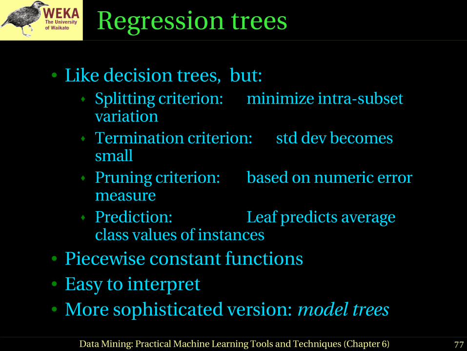
Regression trees
● Like decision trees, but:♦ Splitting criterion: minimize intrasubset
variation♦ Termination criterion: std dev becomes
small♦ Pruning criterion: based on numeric error
measure♦ Prediction: Leaf predicts average
class values of instances● Piecewise constant functions● Easy to interpret● More sophisticated version: model trees
78Data Mining: Practical Machine Learning Tools and Techniques (Chapter 6)
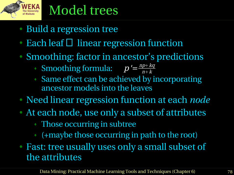
Model trees● Build a regression tree● Each leaf ⇒ linear regression function● Smoothing: factor in ancestor’s predictions
♦ Smoothing formula: ♦ Same effect can be achieved by incorporating
ancestor models into the leaves● Need linear regression function at each node● At each node, use only a subset of attributes
♦ Those occurring in subtree♦ (+maybe those occurring in path to the root)
● Fast: tree usually uses only a small subset of the attributes
p'= npkqnk

79Data Mining: Practical Machine Learning Tools and Techniques (Chapter 6)
Building the tree● Splitting: standard deviation reduction
● Termination:♦ Standard deviation < 5% of its value on full training set♦ Too few instances remain (e.g. < 4)
Pruning:♦ Heuristic estimate of absolute error of LR models:
♦ Greedily remove terms from LR models to minimize estimated error
♦ Heavy pruning: single model may replace whole subtree♦ Proceed bottom up: compare error of LR model at internal
node to error of subtree
SDR=sd T−∑i∣Ti
T∣×sdTi
nn−×average_absolute_error
80Data Mining: Practical Machine Learning Tools and Techniques (Chapter 6)
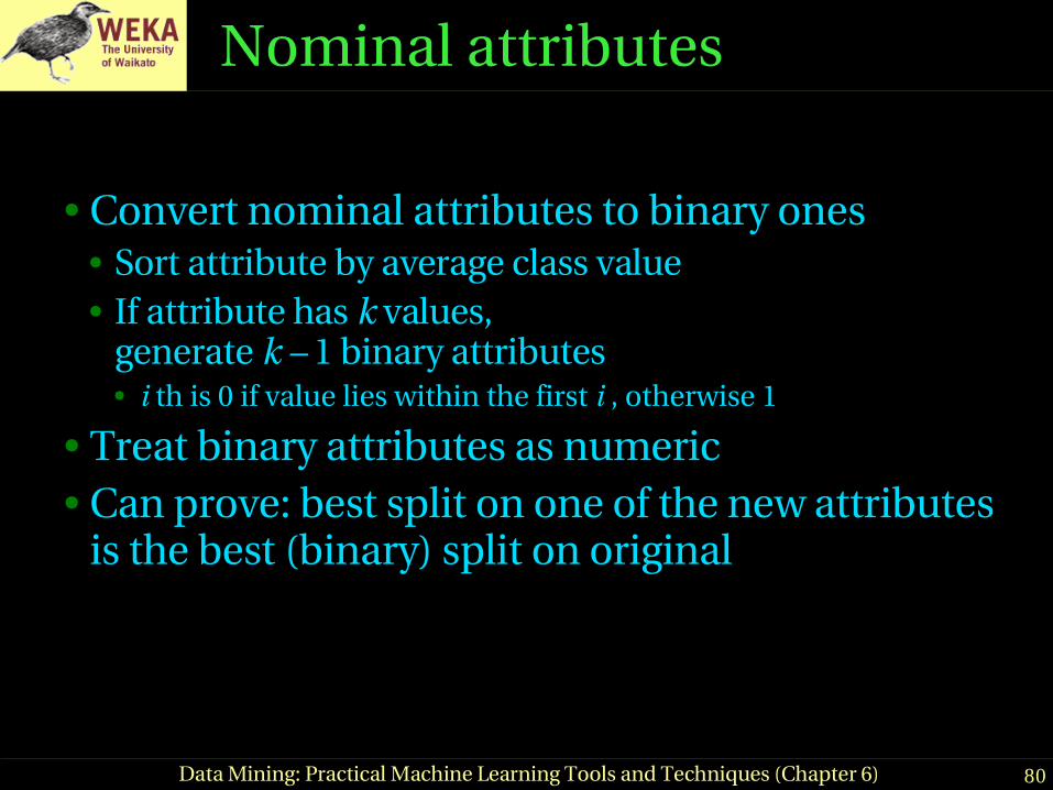
Nominal attributes
● Convert nominal attributes to binary ones● Sort attribute by average class value● If attribute has k values,
generate k – 1 binary attributes● i th is 0 if value lies within the first i , otherwise 1
● Treat binary attributes as numeric● Can prove: best split on one of the new attributes
is the best (binary) split on original
81Data Mining: Practical Machine Learning Tools and Techniques (Chapter 6)
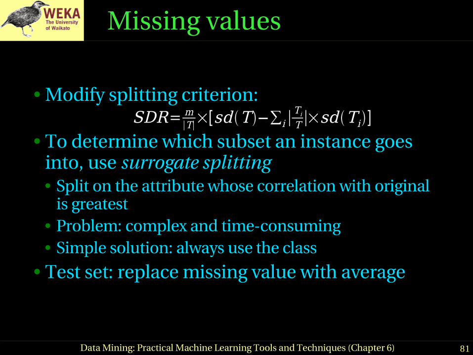
Missing values
● Modify splitting criterion:
● To determine which subset an instance goes into, use surrogate splitting● Split on the attribute whose correlation with original
is greatest● Problem: complex and timeconsuming● Simple solution: always use the class
● Test set: replace missing value with average
SDR= m∣T∣×[sd T−∑i∣
Ti
T ∣×sd Ti]
82Data Mining: Practical Machine Learning Tools and Techniques (Chapter 6)
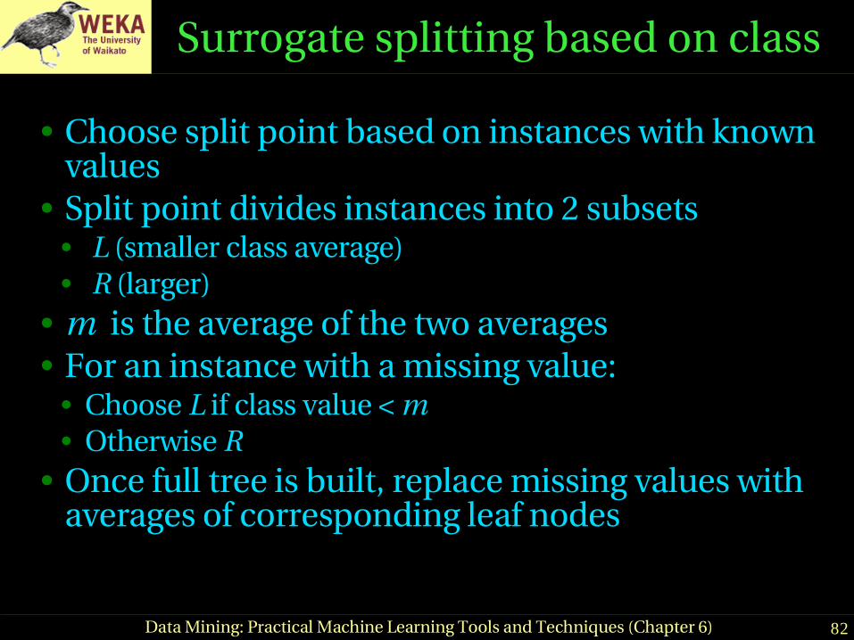
Surrogate splitting based on class
● Choose split point based on instances with known values
● Split point divides instances into 2 subsets● L (smaller class average)● R (larger)
● m is the average of the two averages● For an instance with a missing value:
● Choose L if class value < m● Otherwise R
● Once full tree is built, replace missing values with averages of corresponding leaf nodes

83Data Mining: Practical Machine Learning Tools and Techniques (Chapter 6)
Pseudocode for M5'
● Four methods:♦ Main method: MakeModelTree♦ Method for splitting: split♦ Method for pruning: prune♦ Method that computes error: subtreeError
● We’ll briefly look at each method in turn● Assume that linear regression method performs
attribute subset selection based on error

84Data Mining: Practical Machine Learning Tools and Techniques (Chapter 6)
MakeModelTree
MakeModelTree (instances){ SD = sd(instances) for each k-valued nominal attribute convert into k-1 synthetic binary attributes root = newNode root.instances = instances split(root) prune(root) printTree(root)}
85Data Mining: Practical Machine Learning Tools and Techniques (Chapter 6)
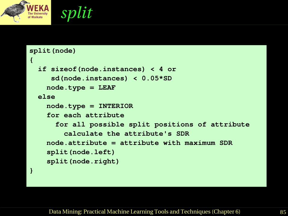
split
split(node) { if sizeof(node.instances) < 4 or sd(node.instances) < 0.05*SD node.type = LEAF else node.type = INTERIOR for each attribute for all possible split positions of attribute calculate the attribute's SDR node.attribute = attribute with maximum SDR split(node.left) split(node.right)}

86Data Mining: Practical Machine Learning Tools and Techniques (Chapter 6)
prune
prune(node){ if node = INTERIOR then prune(node.leftChild) prune(node.rightChild) node.model = linearRegression(node) if subtreeError(node) > error(node) then node.type = LEAF}
87Data Mining: Practical Machine Learning Tools and Techniques (Chapter 6)
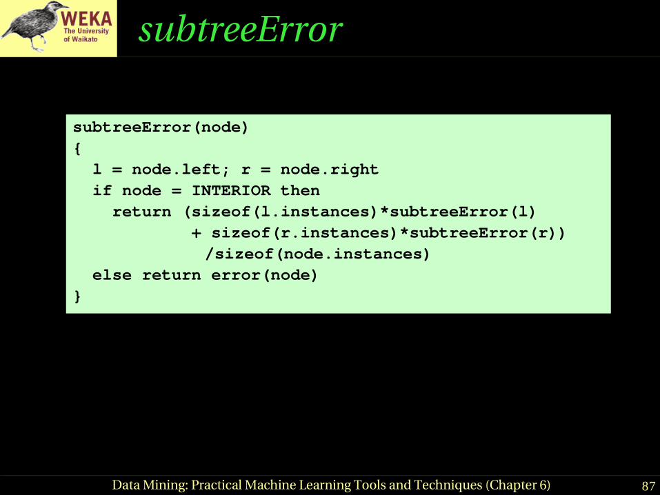
subtreeError
subtreeError(node){ l = node.left; r = node.right if node = INTERIOR then return (sizeof(l.instances)*subtreeError(l) + sizeof(r.instances)*subtreeError(r))
/sizeof(node.instances) else return error(node)}
88Data Mining: Practical Machine Learning Tools and Techniques (Chapter 6)
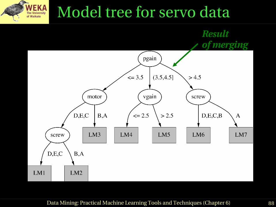
Model tree for servo dataResultof merging
89Data Mining: Practical Machine Learning Tools and Techniques (Chapter 6)
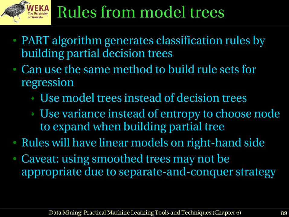
Rules from model trees
● PART algorithm generates classification rules by building partial decision trees
● Can use the same method to build rule sets for regression
♦ Use model trees instead of decision trees♦ Use variance instead of entropy to choose node
to expand when building partial tree● Rules will have linear models on righthand side● Caveat: using smoothed trees may not be
appropriate due to separateandconquer strategy

90Data Mining: Practical Machine Learning Tools and Techniques (Chapter 6)
Locally weighted regression
● Numeric prediction that combines● instancebased learning● linear regression
● “Lazy”:● computes regression function at prediction time● works incrementally
● Weight training instances● according to distance to test instance● needs weighted version of linear regression
● Advantage: nonlinear approximation● But: slow

91Data Mining: Practical Machine Learning Tools and Techniques (Chapter 6)
Design decisions
● Weighting function: ♦ Inverse Euclidean distance♦ Gaussian kernel applied to Euclidean distance♦ Triangular kernel used the same way♦ etc.
● Smoothing parameter is used to scale the distance function
♦ Multiply distance by inverse of this parameter♦ Possible choice: distance of k th nearest training
instance (makes it data dependent)

92Data Mining: Practical Machine Learning Tools and Techniques (Chapter 6)
Discussion
● Regression trees were introduced in CART● Quinlan proposed model tree method (M5)● M5’: slightly improved, publicly available● Quinlan also investigated combining instance
based learning with M5● CUBIST: Quinlan’s commercial rule learner for
numeric prediction● Interesting comparison: neural nets vs. M5

93Data Mining: Practical Machine Learning Tools and Techniques (Chapter 6)
Clustering: how many clusters?
● How to choose k in kmeans? Possibilities:♦ Choose k that minimizes crossvalidated squared
distance to cluster centers♦ Use penalized squared distance on the training
data (eg. using an MDL criterion)♦ Apply kmeans recursively with k = 2 and use
stopping criterion (eg. based on MDL)● Seeds for subclusters can be chosen by seeding along
direction of greatest variance in cluster(one standard deviation away in each direction from cluster center of parent cluster)
● Implemented in algorithm called Xmeans (using Bayesian Information Criterion instead of MDL)
94Data Mining: Practical Machine Learning Tools and Techniques (Chapter 6)
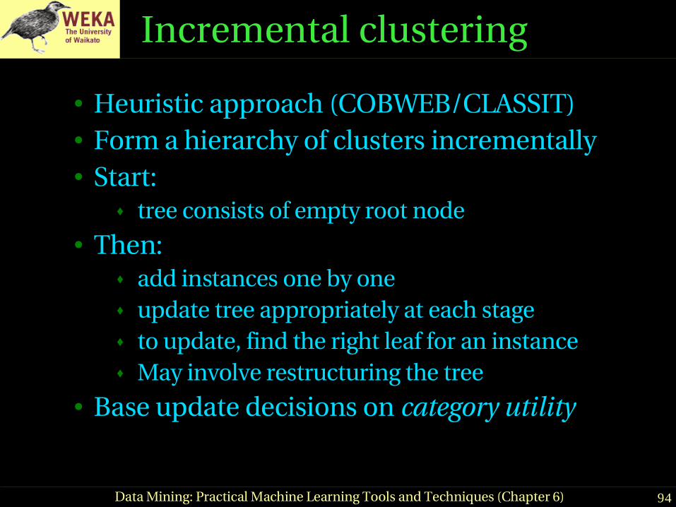
Incremental clustering
● Heuristic approach (COBWEB/CLASSIT)● Form a hierarchy of clusters incrementally● Start:
♦ tree consists of empty root node● Then:
♦ add instances one by one♦ update tree appropriately at each stage♦ to update, find the right leaf for an instance♦ May involve restructuring the tree
● Base update decisions on category utility
95Data Mining: Practical Machine Learning Tools and Techniques (Chapter 6)
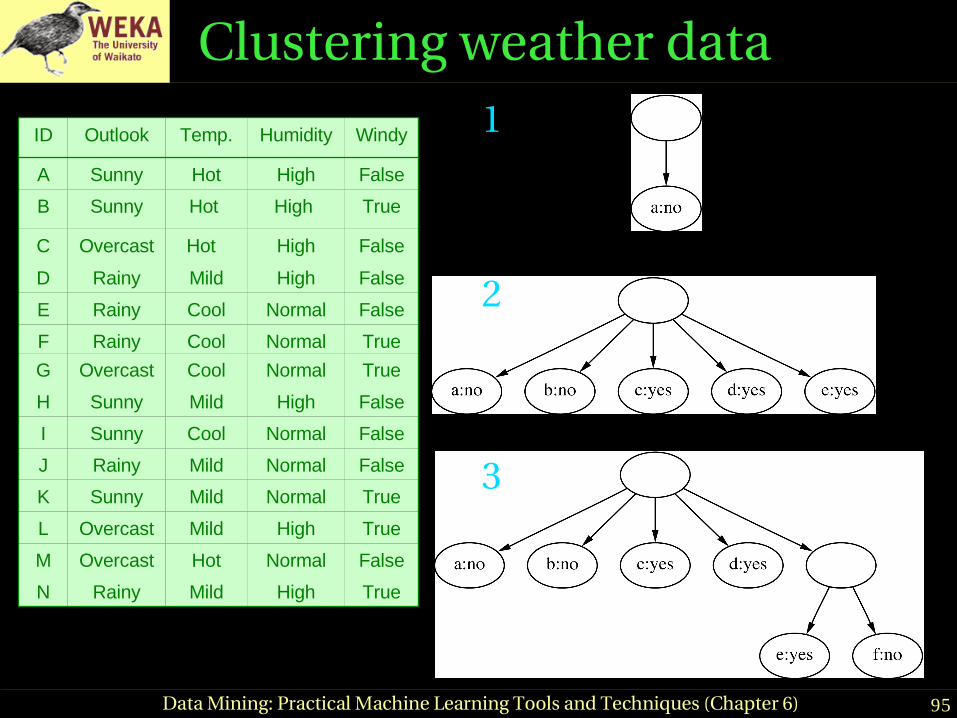
Clustering weather data
N
M
L
K
J
I
H
G
F
E
D
C
B
A
ID
TrueHighMildRainy
FalseNormalHotOvercast
TrueHighMildOvercast
TrueNormalMildSunny
FalseNormalMildRainy
FalseNormalCoolSunny
FalseHighMildSunny
TrueNormalCoolOvercast
TrueNormalCoolRainy
FalseNormalCoolRainy
FalseHighMildRainy
FalseHighHot Overcast
TrueHigh Hot Sunny
FalseHighHotSunny
WindyHumidityTemp.Outlook 1
2
3

96Data Mining: Practical Machine Learning Tools and Techniques (Chapter 6)
Clustering weather data
N
M
L
K
J
I
H
G
F
E
D
C
B
A
ID
TrueHighMildRainy
FalseNormalHotOvercast
TrueHighMildOvercast
TrueNormalMildSunny
FalseNormalMildRainy
FalseNormalCoolSunny
FalseHighMildSunny
TrueNormalCoolOvercast
TrueNormalCoolRainy
FalseNormalCoolRainy
FalseHighMildRainy
FalseHighHot Overcast
TrueHigh Hot Sunny
FalseHighHotSunny
WindyHumidityTemp.Outlook 4
3
Mer ge best host and r unner - up
5
Consider spl i t t i ng the best host if merging doesn’t help
97Data Mining: Practical Machine Learning Tools and Techniques (Chapter 6)
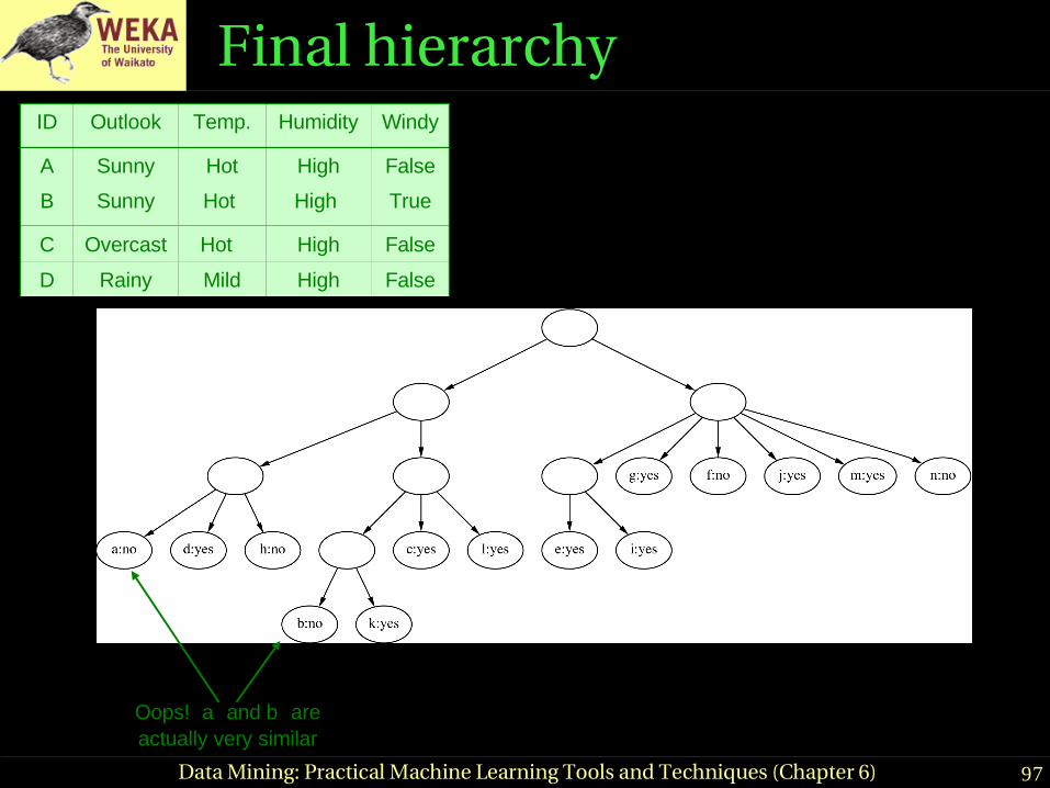
Final hierarchy
D
C
B
A
ID
FalseHighMildRainy
FalseHighHot Overcast
TrueHigh Hot Sunny
FalseHighHotSunny
WindyHumidityTemp.Outlook
Oops! a and b are actually very similar

98Data Mining: Practical Machine Learning Tools and Techniques (Chapter 6)
Example: the iris data (subset)
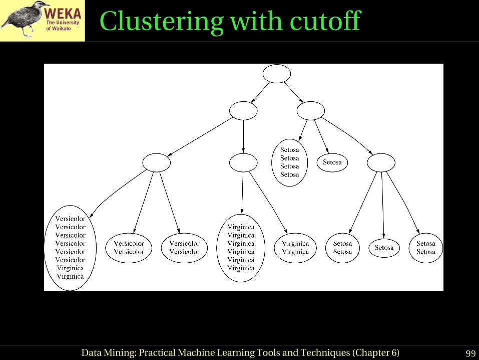
99Data Mining: Practical Machine Learning Tools and Techniques (Chapter 6)
Clustering with cutoff

100Data Mining: Practical Machine Learning Tools and Techniques (Chapter 6)
Category utility
● Category utility: quadratic loss functiondefined on conditional probabilities:
● Every instance in different category ⇒ numerator becomes
maximum
number of attributes
CUC1,C2, ... ,Ck=∑l Pr [Cl ]∑i ∑ j Pr [ai=vij |Cl ]
2−Pr [ai=v ij]2
k
n−∑i ∑ j Pr [ai=v ij]2

101Data Mining: Practical Machine Learning Tools and Techniques (Chapter 6)
Numeric attributes● Assume normal distribution:
● Then:
● Thus
becomes
● Prespecified minimum variance♦ acuity parameter
f a= 1
2exp − a−2
22
∑ j Pr [ai=vij]2≡∫ f ai
2dai=1
2 i
CUC1,C2,... ,Ck =∑l Pr [Cl ]∑i ∑ j Pr [ai=vij |Cl]
2−Pr [ai=v ij]2
k
CUC1,C2, ... ,Ck=∑l Pr [Cl ]
12 ∑i
1 il− 1
i
k

102Data Mining: Practical Machine Learning Tools and Techniques (Chapter 6)
Probabilitybased clustering
● Problems with heuristic approach:♦ Division by k?♦ Order of examples?♦ Are restructuring operations sufficient?♦ Is result at least local minimum of category
utility?
● Probabilistic perspective ⇒seek the most likely clusters given the data
● Also: instance belongs to a particular cluster with a certain probability
103Data Mining: Practical Machine Learning Tools and Techniques (Chapter 6)
Finite mixtures
● Model data using a mixture of distributions● One cluster, one distribution
♦ governs probabilities of attribute values in that cluster● Finite mixtures : finite number of clusters● Individual distributions are normal (usually)● Combine distributions using cluster weights
104Data Mining: Practical Machine Learning Tools and Techniques (Chapter 6)
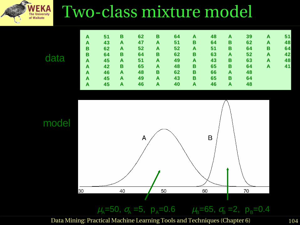
Twoclass mixture modelA 51A 43B 62B 64A 45A 42A 46A 45A 45
B 62A 47A 52B 64A 51B 65A 48A 49A 46
B 64A 51A 52B 62A 49A 48B 62A 43A 40
A 48B 64A 51B 63A 43B 65B 66B 65A 46
A 39B 62B 64A 52B 63B 64A 48B 64A 48
A 51A 48B 64A 42A 48A 41
data
model
µA=50, σA =5, pA=0.6 µB=65, σB =2, pB=0.4

105Data Mining: Practical Machine Learning Tools and Techniques (Chapter 6)
Using the mixture model
● Probability that instance x belongs to cluster A:
with
● Probability of an instance given the clusters:
Pr [A |x ]= Pr [x |A ]Pr [A ]Pr [x ] = f x ;A ,A pA
Pr [x ]
f x ; ,= 1
2exp − x−2
22
Pr [x|the_clusters]=∑i Pr [x|clusteri ]Pr [clusteri ]
106Data Mining: Practical Machine Learning Tools and Techniques (Chapter 6)
Learning the clusters
● Assume:♦ we know there are k clusters
● Learn the clusters ⇒♦ determine their parameters♦ I.e. means and standard deviations
● Performance criterion:♦ probability of training data given the clusters
● EM algorithm♦ finds a local maximum of the likelihood

107Data Mining: Practical Machine Learning Tools and Techniques (Chapter 6)
EM algorithm
● EM = ExpectationMaximization ● Generalize kmeans to probabilistic setting
● Iterative procedure:● E “expectation” step:
Calculate cluster probability for each instance ● M “maximization” step:
Estimate distribution parameters from cluster probabilities
● Store cluster probabilities as instance weights● Stop when improvement is negligible

108Data Mining: Practical Machine Learning Tools and Techniques (Chapter 6)
More on EM
● Estimate parameters from weighted instances
● Stop when loglikelihood saturates
● Loglikelihood:
A=w1 x1w2 x2...wn xn
w1w2...wn
A=w1x1−2w2x2−2...wn xn−2
w1w2...wn
∑i log pA Pr [xi | A ]pBPr [xi |B]
109Data Mining: Practical Machine Learning Tools and Techniques (Chapter 6)
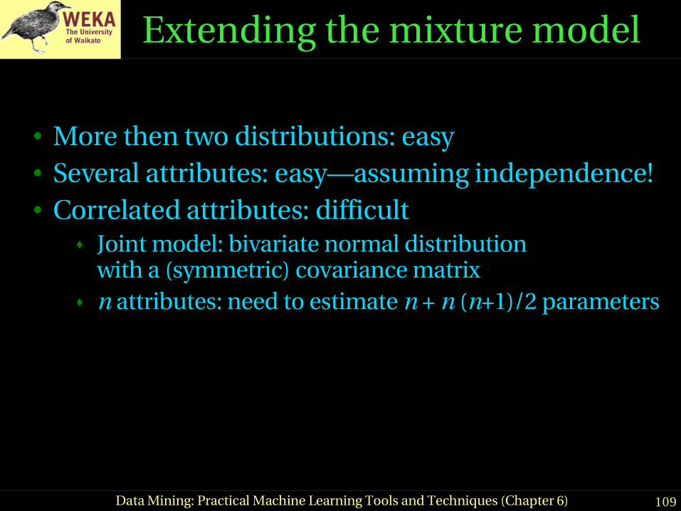
Extending the mixture model
● More then two distributions: easy● Several attributes: easy—assuming independence!● Correlated attributes: difficult
♦ Joint model: bivariate normal distributionwith a (symmetric) covariance matrix
♦ n attributes: need to estimate n + n (n+1)/2 parameters
110Data Mining: Practical Machine Learning Tools and Techniques (Chapter 6)
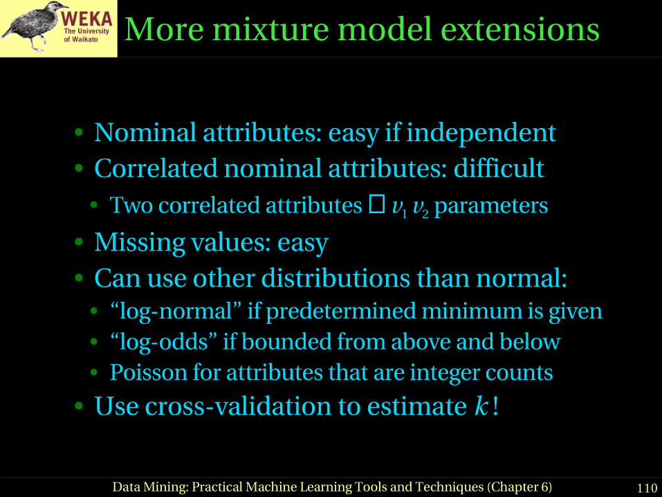
More mixture model extensions
● Nominal attributes: easy if independent● Correlated nominal attributes: difficult
● Two correlated attributes ⇒ v1 v2 parameters
● Missing values: easy● Can use other distributions than normal:
● “lognormal” if predetermined minimum is given● “logodds” if bounded from above and below● Poisson for attributes that are integer counts
● Use crossvalidation to estimate k !

111Data Mining: Practical Machine Learning Tools and Techniques (Chapter 6)
Bayesian clustering
● Problem: many parameters ⇒ EM overfits● Bayesian approach : give every parameter a prior
probability distribution♦ Incorporate prior into overall likelihood figure♦ Penalizes introduction of parameters
● Eg: Laplace estimator for nominal attributes● Can also have prior on number of clusters!● Implementation: NASA’s AUTOCLASS
112Data Mining: Practical Machine Learning Tools and Techniques (Chapter 6)
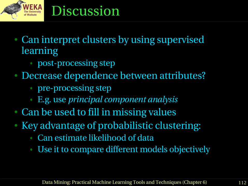
Discussion
● Can interpret clusters by using supervised learning
♦ postprocessing step● Decrease dependence between attributes?
♦ preprocessing step♦ E.g. use principal component analysis
● Can be used to fill in missing values● Key advantage of probabilistic clustering:
♦ Can estimate likelihood of data♦ Use it to compare different models objectively

113Data Mining: Practical Machine Learning Tools and Techniques (Chapter 6)
From naïve Bayes to Bayesian Networks
● Naïve Bayes assumes:attributes conditionally independent given the class
● Doesn’t hold in practice but classification accuracy often high
● However: sometimes performance much worse than e.g. decision tree
● Can we eliminate the assumption?

114Data Mining: Practical Machine Learning Tools and Techniques (Chapter 6)
Enter Bayesian networks
● Graphical models that can represent any probability distribution
● Graphical representation: directed acyclic graph, one node for each attribute
● Overall probability distribution factorized into component distributions
● Graph’s nodes hold component distributions (conditional distributions)

115Data Mining: Practical Machine Learning Tools and Techniques (Chapter 6)
Net
work
for t
he
wea
ther
dat
a

116Data Mining: Practical Machine Learning Tools and Techniques (Chapter 6)
Net
work
for t
he
wea
ther
dat
a

117Data Mining: Practical Machine Learning Tools and Techniques (Chapter 6)
Computing the class probabilities
● Two steps: computing a product of probabilities for each class and normalization
♦ For each class value● Take all attribute values and class value● Look up corresponding entries in conditional
probability distribution tables● Take the product of all probabilities
♦ Divide the product for each class by the sum of the products (normalization)
118Data Mining: Practical Machine Learning Tools and Techniques (Chapter 6)
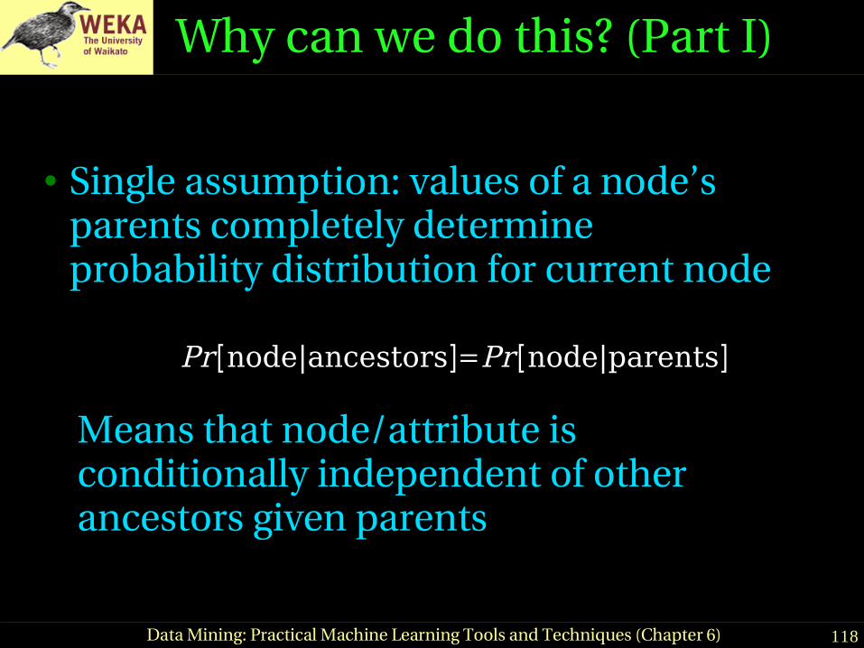
Why can we do this? (Part I)
● Single assumption: values of a node’s parents completely determine probability distribution for current node
• Means that node/attribute is conditionally independent of other ancestors given parents
Pr [node|ancestors]=Pr [node|parents]

119Data Mining: Practical Machine Learning Tools and Techniques (Chapter 6)
Why can we do this? (Part II)
● Chain rule from probability theory:
• Because of our assumption from the previous slide:
Pr [a1,a2,... ,an]=∏i=1n Pr [ai|ai−1 , ... ,a1]
Pr [a1,a2,... ,an]=∏i=1n Pr [ai|ai−1 , ... ,a1]=
∏i=1n Pr [ai |ai 'sparents]

120Data Mining: Practical Machine Learning Tools and Techniques (Chapter 6)
Learning Bayes nets● Basic components of algorithms for learning
Bayes nets:♦ Method for evaluating the goodness of a given
network● Measure based on probability of training data
given the network (or the logarithm thereof)♦ Method for searching through space of possible
networks● Amounts to searching through sets of edges
because nodes are fixed

121Data Mining: Practical Machine Learning Tools and Techniques (Chapter 6)
Problem: overfitting● Can’t just maximize probability of the training
data♦ Because then it’s always better to add more edges (fit
the training data more closely)● Need to use crossvalidation or some penalty for
complexity of the network– AIC measure:
– MDL measure:
– LL: loglikelihood (log of probability of data), K: number of free parameters, N: #instances
• Another possibility: Bayesian approach with prior distribution over networks
AICscore=−LLK
MDLscore=−LLK2 logN

122Data Mining: Practical Machine Learning Tools and Techniques (Chapter 6)
Searching for a good structure
● Task can be simplified: can optimize each node separately
♦ Because probability of an instance is product of individual nodes’ probabilities
♦ Also works for AIC and MDL criterion because penalties just add up
● Can optimize node by adding or removing edges from other nodes
● Must not introduce cycles!
123Data Mining: Practical Machine Learning Tools and Techniques (Chapter 6)
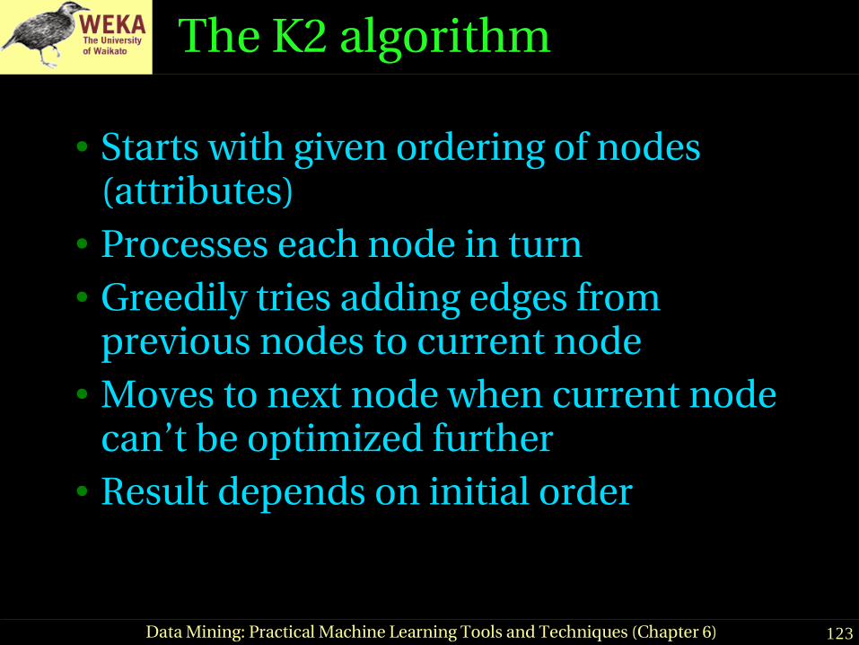
The K2 algorithm
● Starts with given ordering of nodes (attributes)
● Processes each node in turn● Greedily tries adding edges from
previous nodes to current node● Moves to next node when current node
can’t be optimized further● Result depends on initial order

124Data Mining: Practical Machine Learning Tools and Techniques (Chapter 6)
Some tricks
● Sometimes it helps to start the search with a naïve Bayes network
● It can also help to ensure that every node is in Markov blanket of class node
♦ Markov blanket of a node includes all parents, children, and children’s parents of that node
♦ Given values for Markov blanket, node is conditionally independent of nodes outside blanket
♦ I.e. node is irrelevant to classification if not in Markov blanket of class node

125Data Mining: Practical Machine Learning Tools and Techniques (Chapter 6)
Other algorithms
● Extending K2 to consider greedily adding or deleting edges between any pair of nodes
♦ Further step: considering inverting the direction of edges
● TAN (Tree Augmented Naïve Bayes): ♦ Starts with naïve Bayes♦ Considers adding second parent to each node
(apart from class node)♦ Efficient algorithm exists

126Data Mining: Practical Machine Learning Tools and Techniques (Chapter 6)
Likelihood vs. conditional likelihood
● In classification what we really want is to maximize probability of class given other attributes
– Not probability of the instances● But: no closedform solution for probabilities in
nodes’ tables that maximize this● However: can easily compute conditional
probability of data based on given network● Seems to work well when used for network scoring

127Data Mining: Practical Machine Learning Tools and Techniques (Chapter 6)
Data structures for fast learning
● Learning Bayes nets involves a lot of counting for computing conditional probabilities
● Naïve strategy for storing counts: hash table♦ Runs into memory problems very quickly
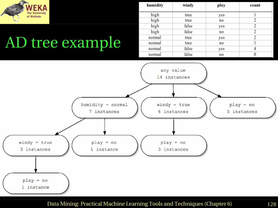
● More sophisticated strategy: alldimensions (AD) tree♦ Analogous to kDtree for numeric data♦ Stores counts in a tree but in a clever way such that
redundancy is eliminated♦ Only makes sense to use it for large datasets
128Data Mining: Practical Machine Learning Tools and Techniques (Chapter 6)
AD tree example
129Data Mining: Practical Machine Learning Tools and Techniques (Chapter 6)
Building an AD tree
● Assume each attribute in the data has been assigned an index
● Then, expand node for attribute i with the values of all attributes j > i
♦ Two important restrictions:● Most populous expansion for each attribute is
omitted (breaking ties arbitrarily)● Expansions with counts that are zero are also
omitted
● The root node is given index zero

130Data Mining: Practical Machine Learning Tools and Techniques (Chapter 6)
Discussion
● We have assumed: discrete data, no missing values, no new nodes
● Different method of using Bayes nets for classification: Bayesian multinets
♦ I.e. build one network for each class and make prediction using Bayes’ rule
● Different class of learning methods for Bayes nets: testing conditional independence assertions
● Can also build Bayes nets for regression tasks