DATA ANALYSIS - THE DATA TABLE WAY

INTRODUCTION

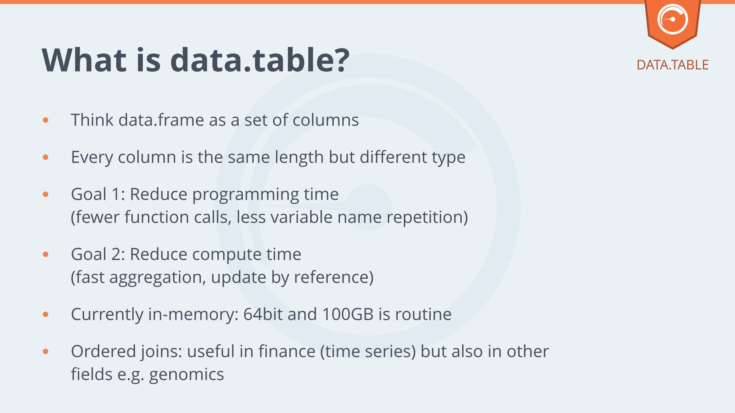
What is data.table?● Think data.frame as a set of columns

● Every column is the same length but different type

● Goal 1: Reduce programming time(fewer function calls, less variable name repetition)

● Goal 2: Reduce compute time(fast aggregation, update by reference)

● Currently in-memory: 64bit and 100GB is routine

● Ordered joins: useful in finance (time series) but also in other fields e.g. genomics

DATA.TABLE

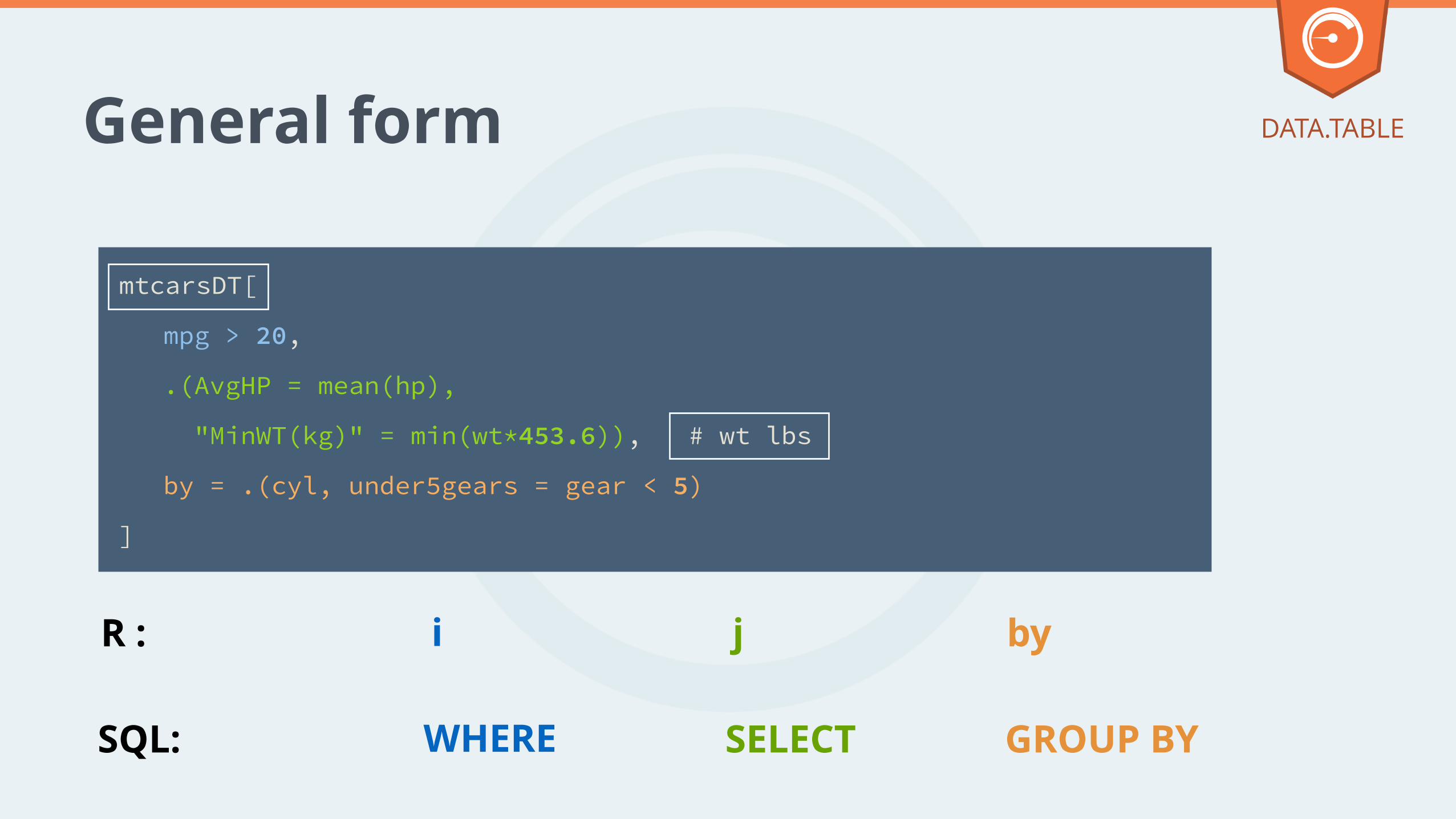
mtcarsDT[

!

!

!

!

]

R :

General form

i j by

DATA.TABLE

!

mpg > 20,

.(AvgHP = mean(hp),

"MinWT(kg)" = min(wt*453.6)), # wt lbs

by = .(cyl, under5gears = gear < 5)

SQL: WHERE SELECT GROUP BY

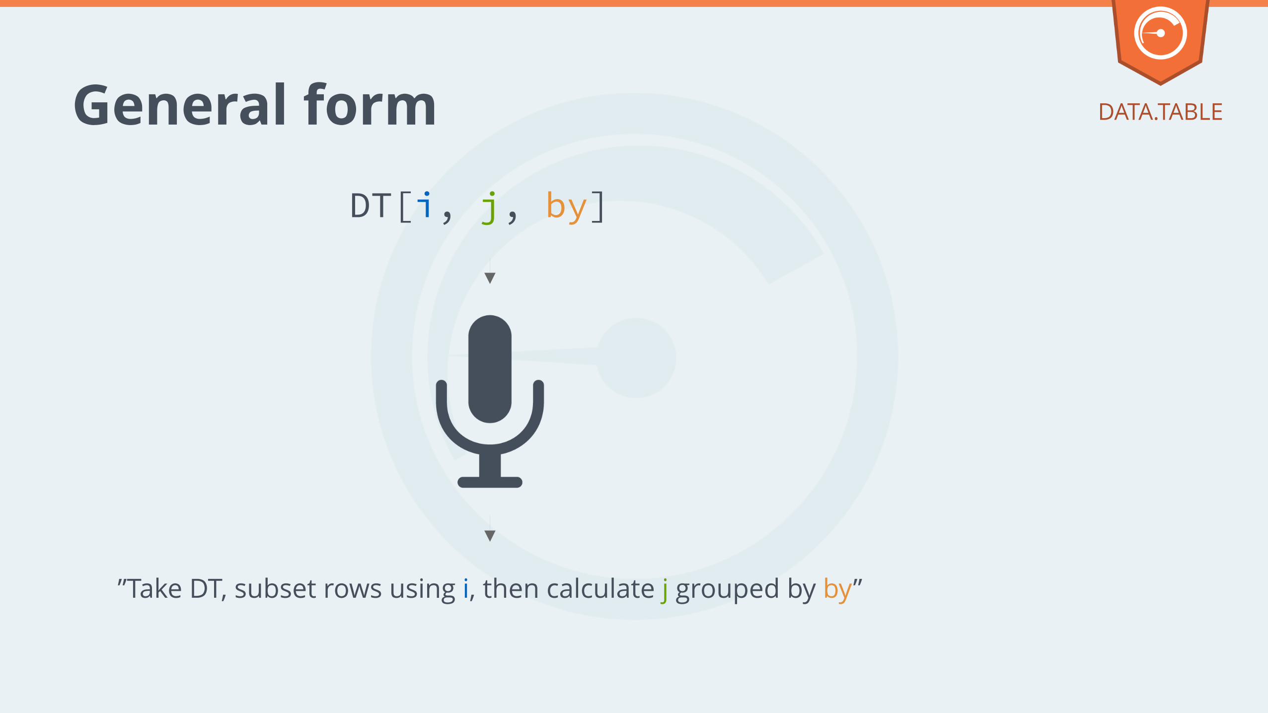
”Take DT, subset rows using i, then calculate j grouped by by”

DT[i, j, by]

General form DATA.TABLE

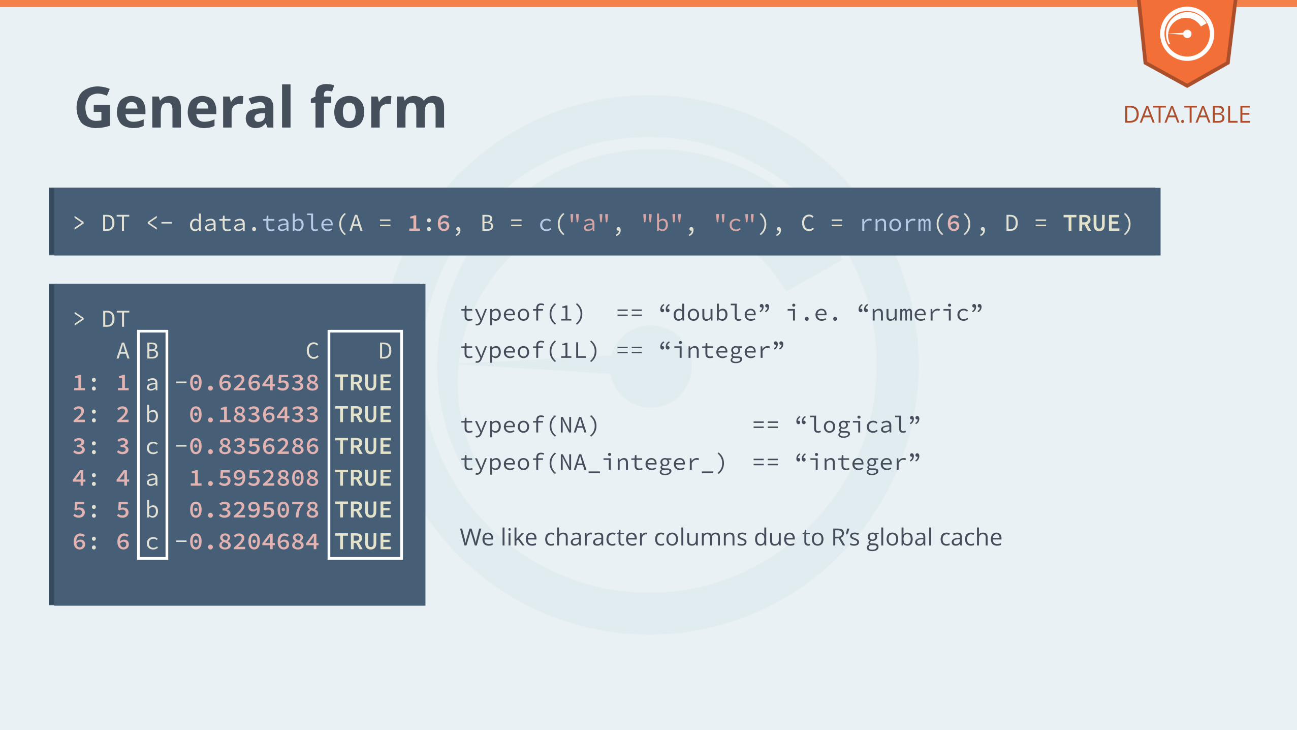
General form

> DT <- data.table(A = 1:6, B = c("a", "b", "c"), C = rnorm(6), D = TRUE)

typeof(1) == “double” i.e. “numeric”typeof(1L) == “integer” !

typeof(NA) == “logical” typeof(NA_integer_) == “integer” !

We like character columns due to R’s global cache

> DT A B C D 1: 1 a -0.6264538 TRUE 2: 2 b 0.1836433 TRUE 3: 3 c -0.8356286 TRUE 4: 4 a 1.5952808 TRUE 5: 5 b 0.3295078 TRUE 6: 6 c -0.8204684 TRUE

DATA.TABLE

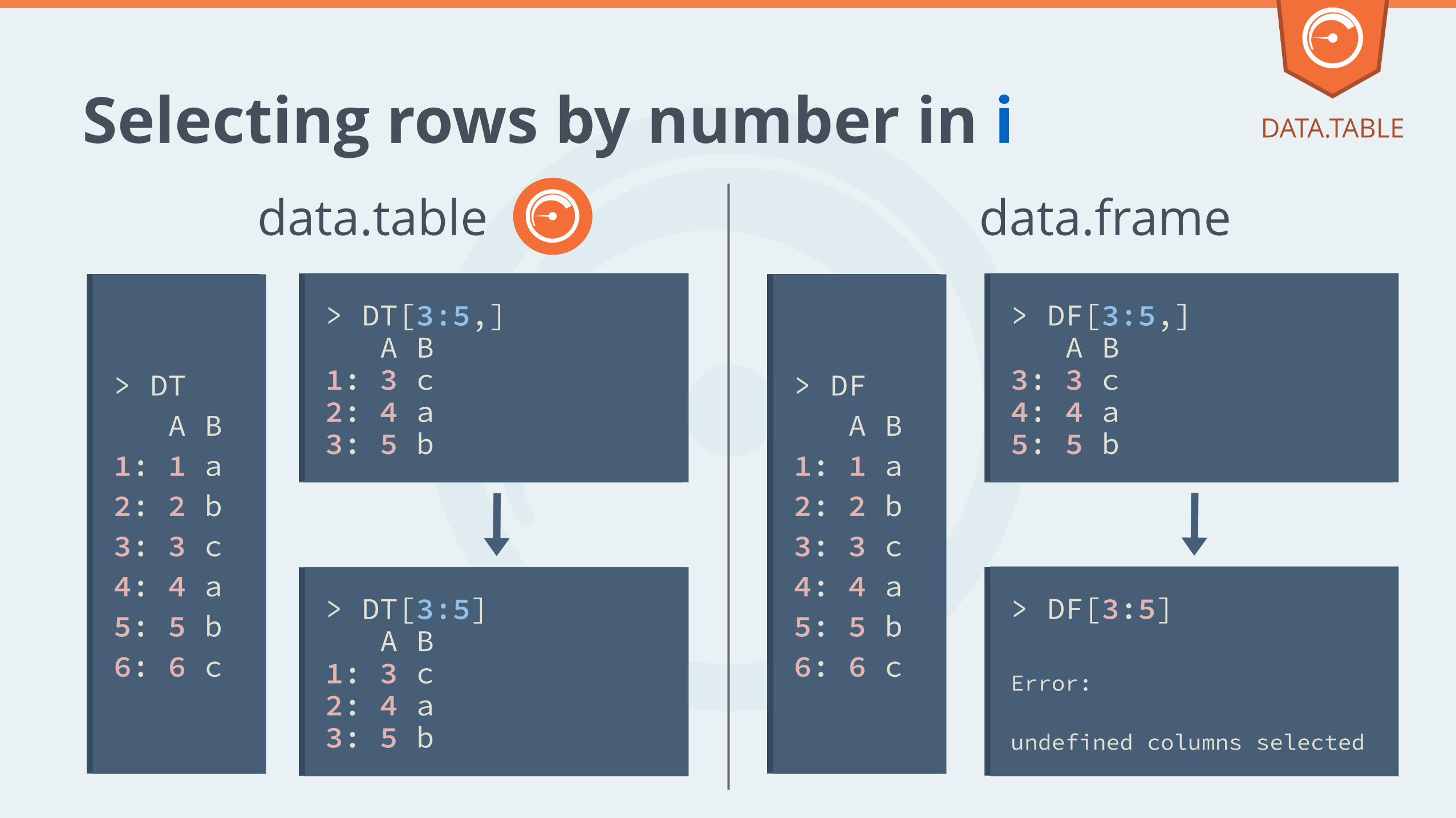
Selecting rows by number in i

> DT A B 1: 1 a 2: 2 b 3: 3 c 4: 4 a 5: 5 b 6: 6 c

> DT[3:5,] A B 1: 3 c 2: 4 a 3: 5 b

> DT[3:5] A B 1: 3 c 2: 4 a 3: 5 b

> DF[3:5]

Error:

undefined columns selected

> DF A B 1: 1 a 2: 2 b 3: 3 c 4: 4 a 5: 5 b 6: 6 c

> DF[3:5,] A B 3: 3 c 4: 4 a 5: 5 b

DATA.TABLE

data.table data.frame

Compatibility

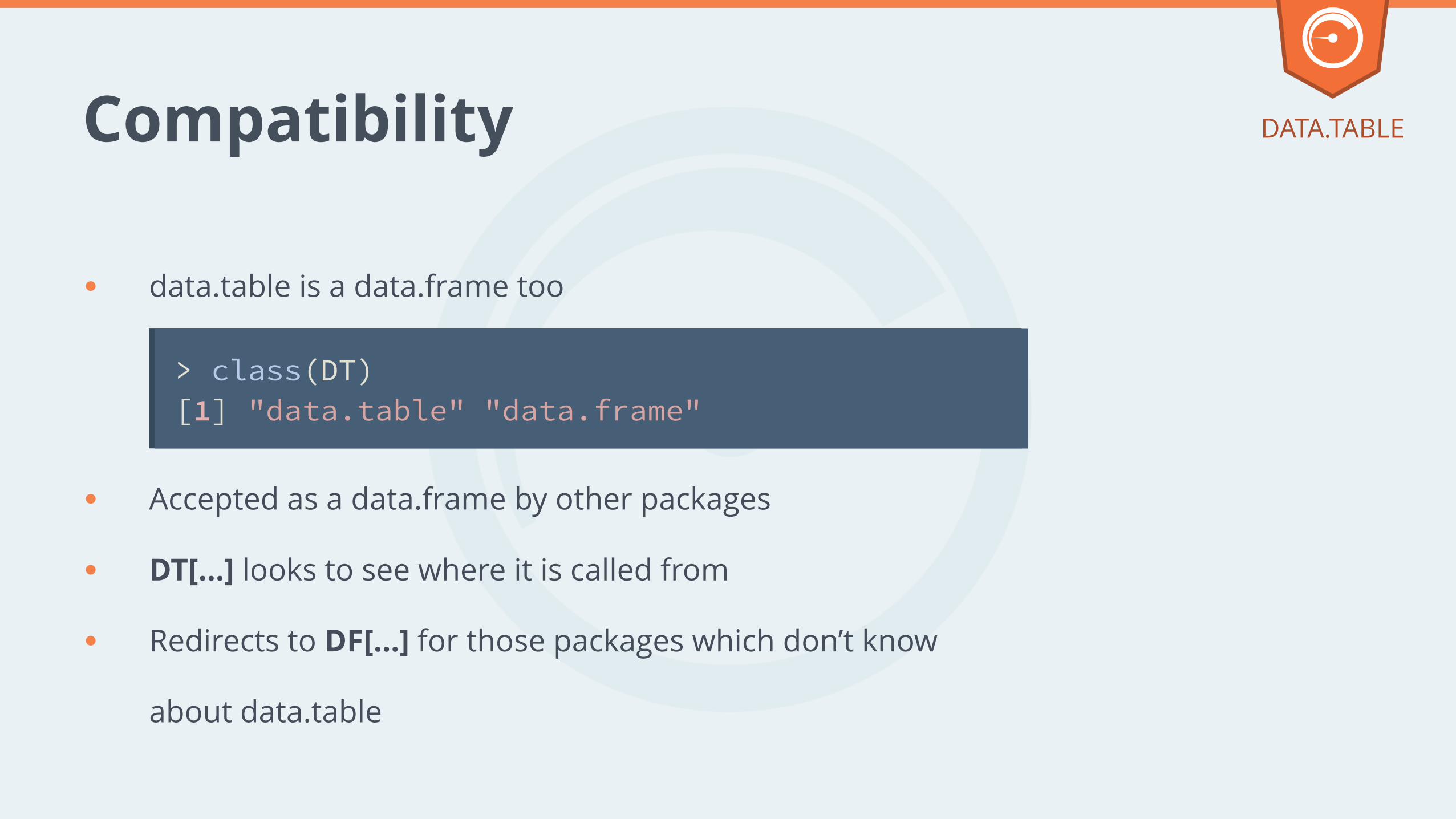
● data.table is a data.frame too

● Accepted as a data.frame by other packages

● DT[...] looks to see where it is called from

● Redirects to DF[...] for those packages which don’t know

about data.table

> class(DT) [1] "data.table" "data.frame"

DATA.TABLE

Let’s practice

DATA.TABLE

DATA ANALYSIS - THE DATA TABLE WAY

SELECTING COLUMNS IN J

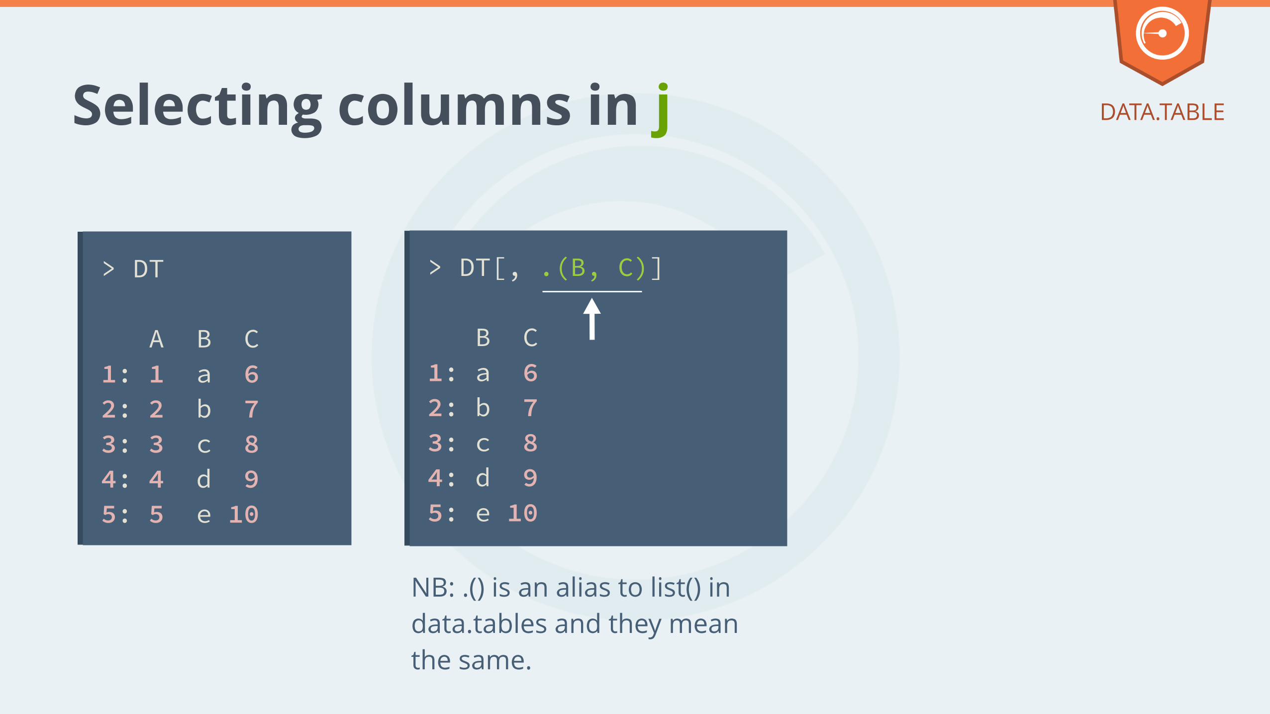
Selecting columns in j

> DT

A B C 1: 1 a 6 2: 2 b 7 3: 3 c 8 4: 4 d 9 5: 5 e 10

> DT[, .(B, C)] B C 1: a 6 2: b 7 3: c 8 4: d 9 5: e 10

DATA.TABLE

NB: .() is an alias to list() in data.tables and they mean the same.

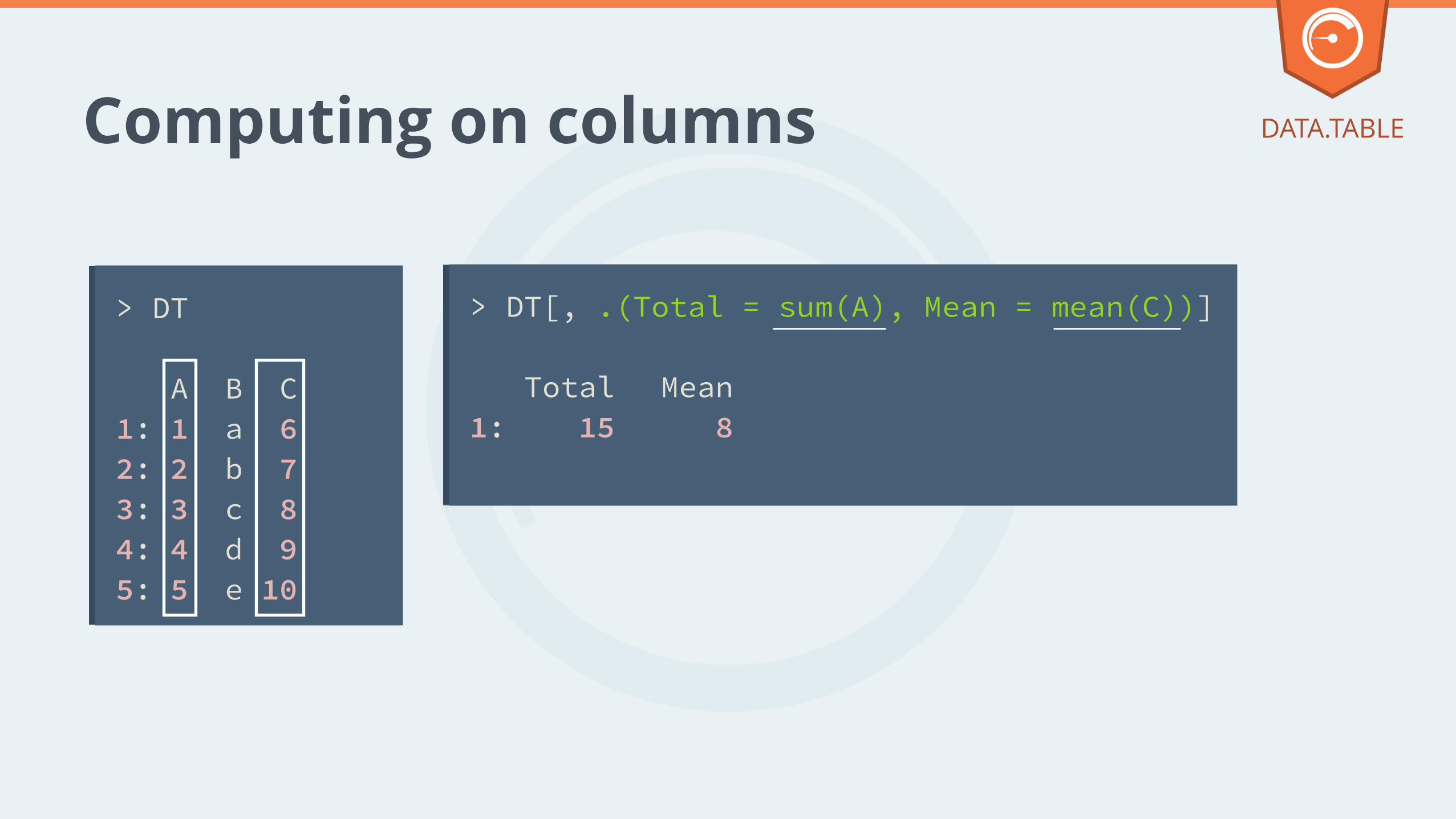
Computing on columns

> DT[, .(Total = sum(A), Mean = mean(C))]

Total Mean 1: 15 8

DATA.TABLE

> DT

A B C 1: 1 a 6 2: 2 b 7 3: 3 c 8 4: 4 d 9 5: 5 e 10

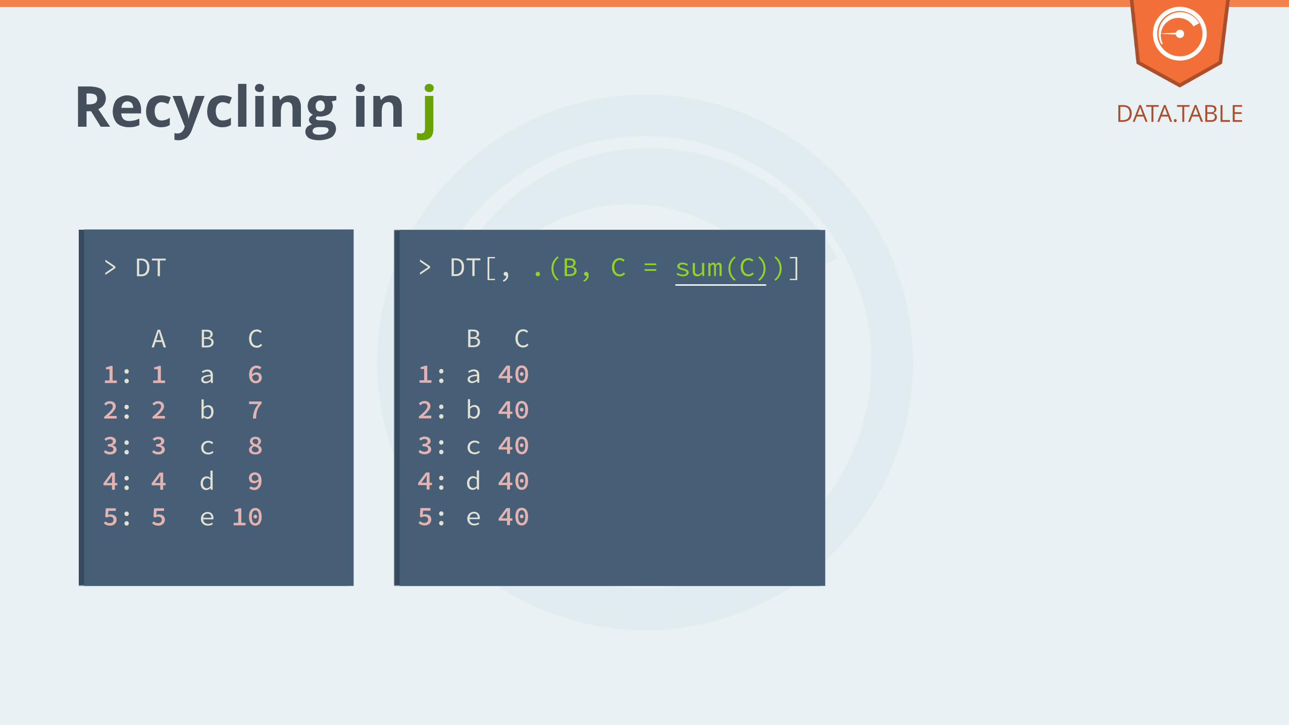
DATA.TABLE Recycling in j

> DT[, .(B, C = sum(C))]

B C 1: a 40 2: b 40 3: c 40 4: d 40 5: e 40

> DT

A B C 1: 1 a 6 2: 2 b 7 3: 3 c 8 4: 4 d 9 5: 5 e 10

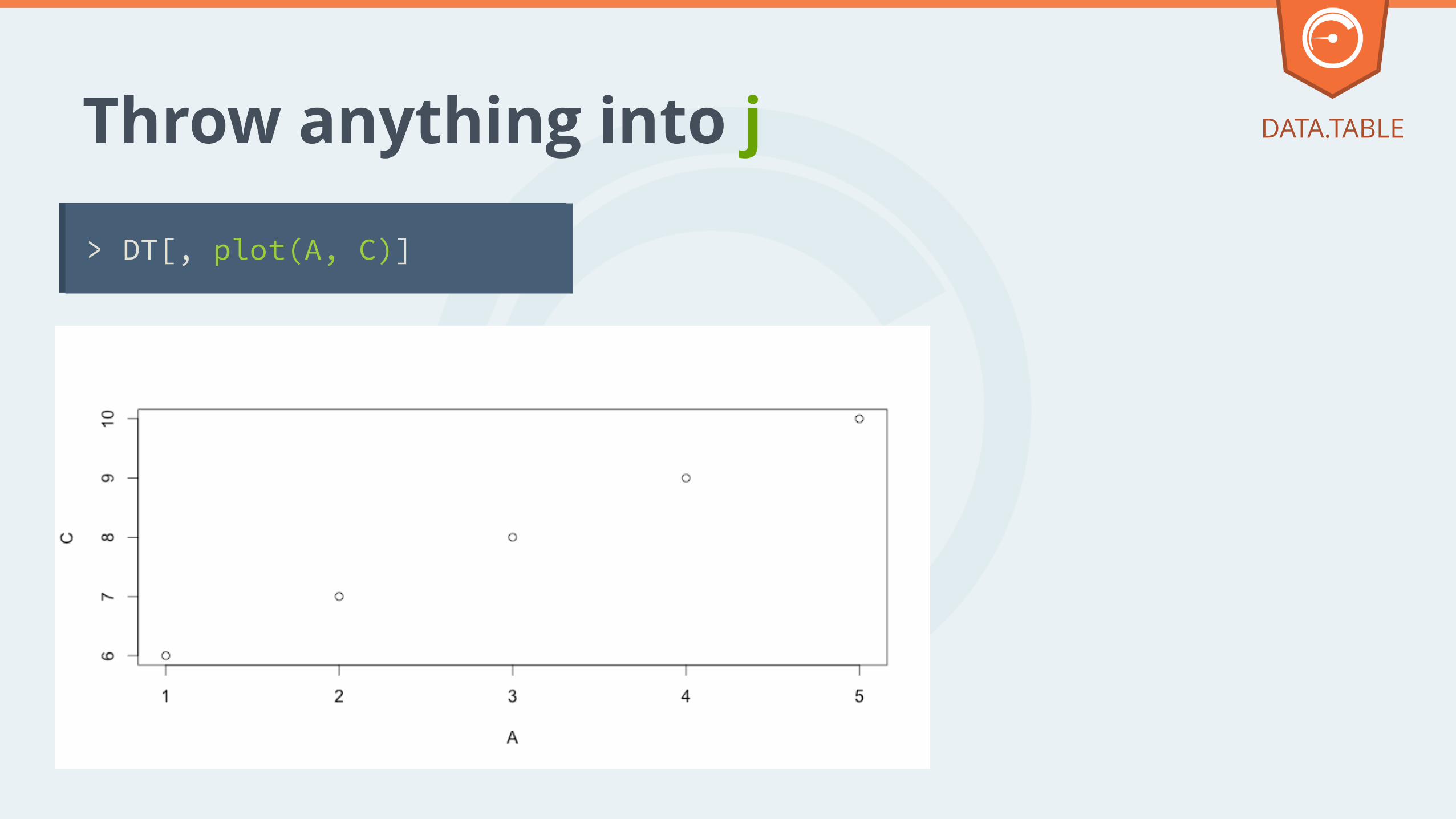
DATA.TABLE Throw anything into j

> DT[, plot(A, C)]

DATA.TABLE

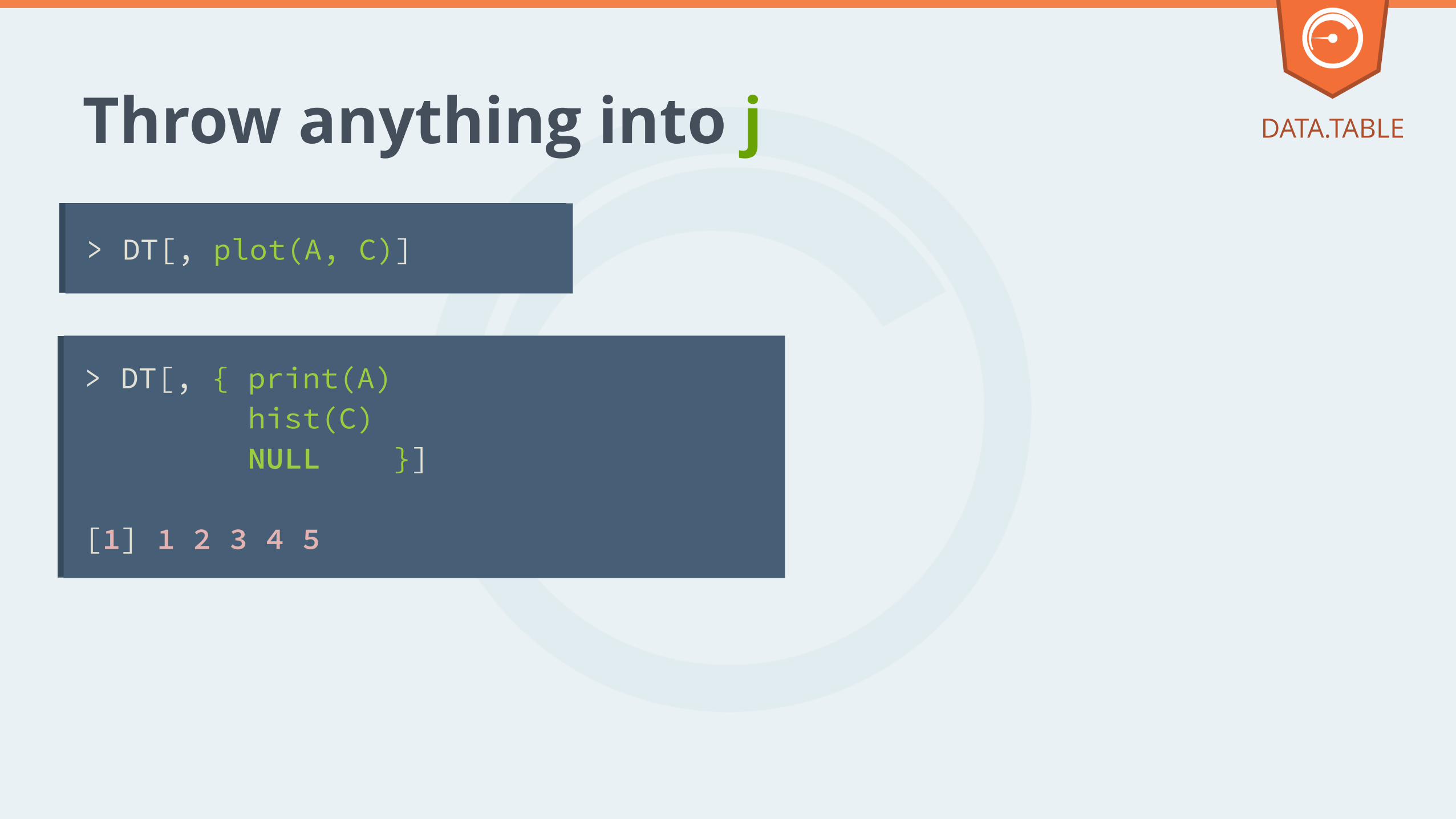
> DT[, plot(A, C)]

Throw anything into j

> DT[, { print(A) hist(C) NULL }]

[1] 1 2 3 4 5

Let’s practice

DATA.TABLE

DATA ANALYSIS - THE DATA TABLE WAY

DOING J BY GROUP

Doing j by group

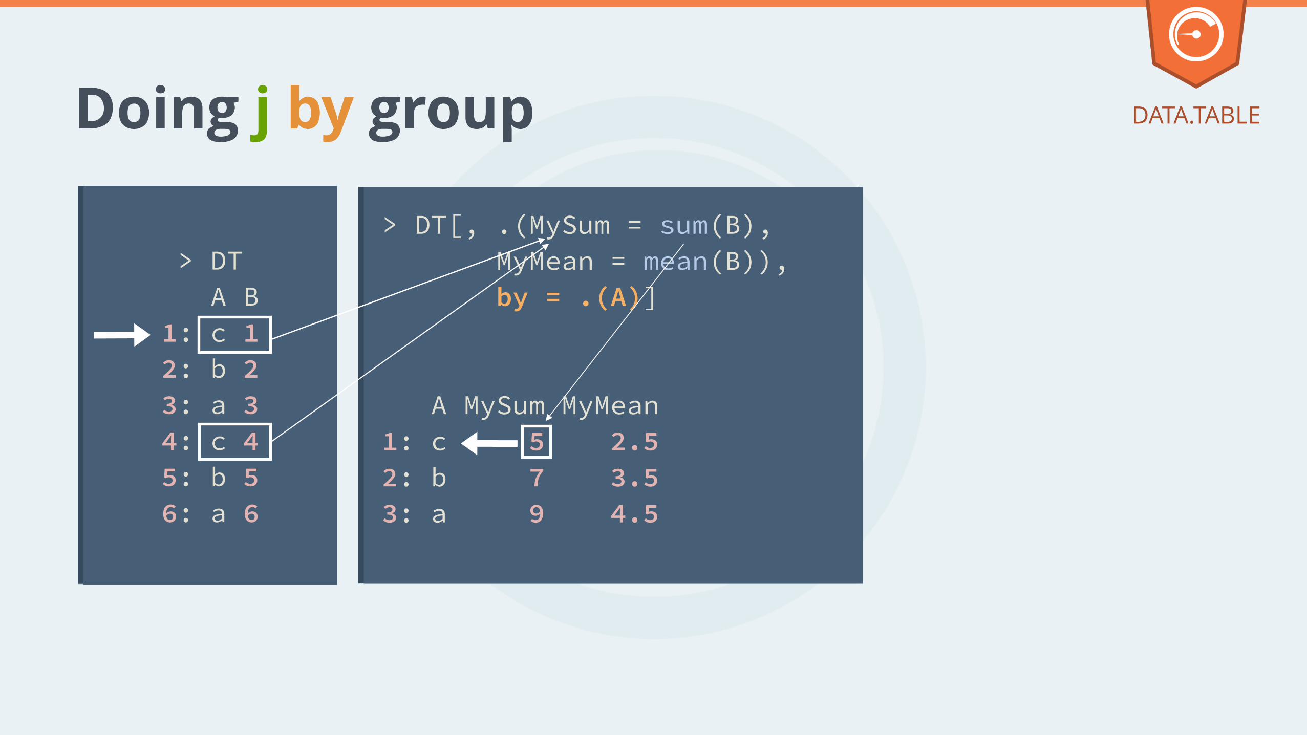
> DT[, .(MySum = sum(B), MyMean = mean(B)), by = .(A)]

A MySum MyMean 1: c 5 2.5 2: b 7 3.5 3: a 9 4.5

> DT A B 1: c 1 2: b 2 3: a 3 4: c 4 5: b 5 6: a 6

DATA.TABLE

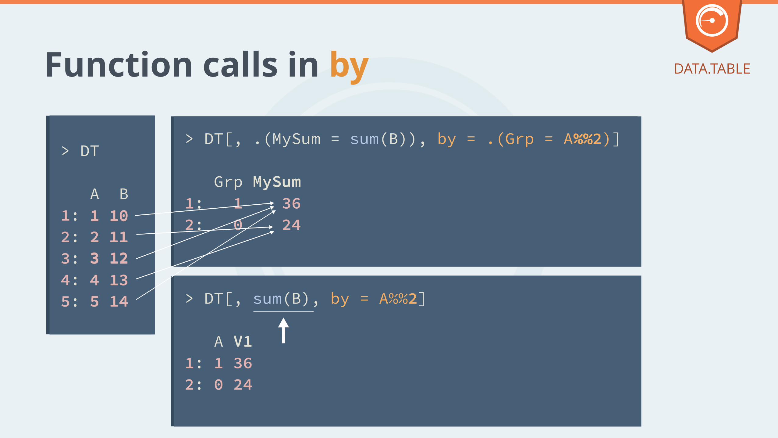
Function calls in by

> DT[, .(MySum = sum(B)), by = .(Grp = A%%2)]

Grp MySum 1: 1 36 2: 0 24

> DT[, sum(B), by = A%%2]

A V1 1: 1 36 2: 0 24

> DT

A B 1: 1 10 2: 2 11 3: 3 12 4: 4 13 5: 5 14

DATA.TABLE

%%

1

3

5

10

12

144

2 11

13

MySum

V1

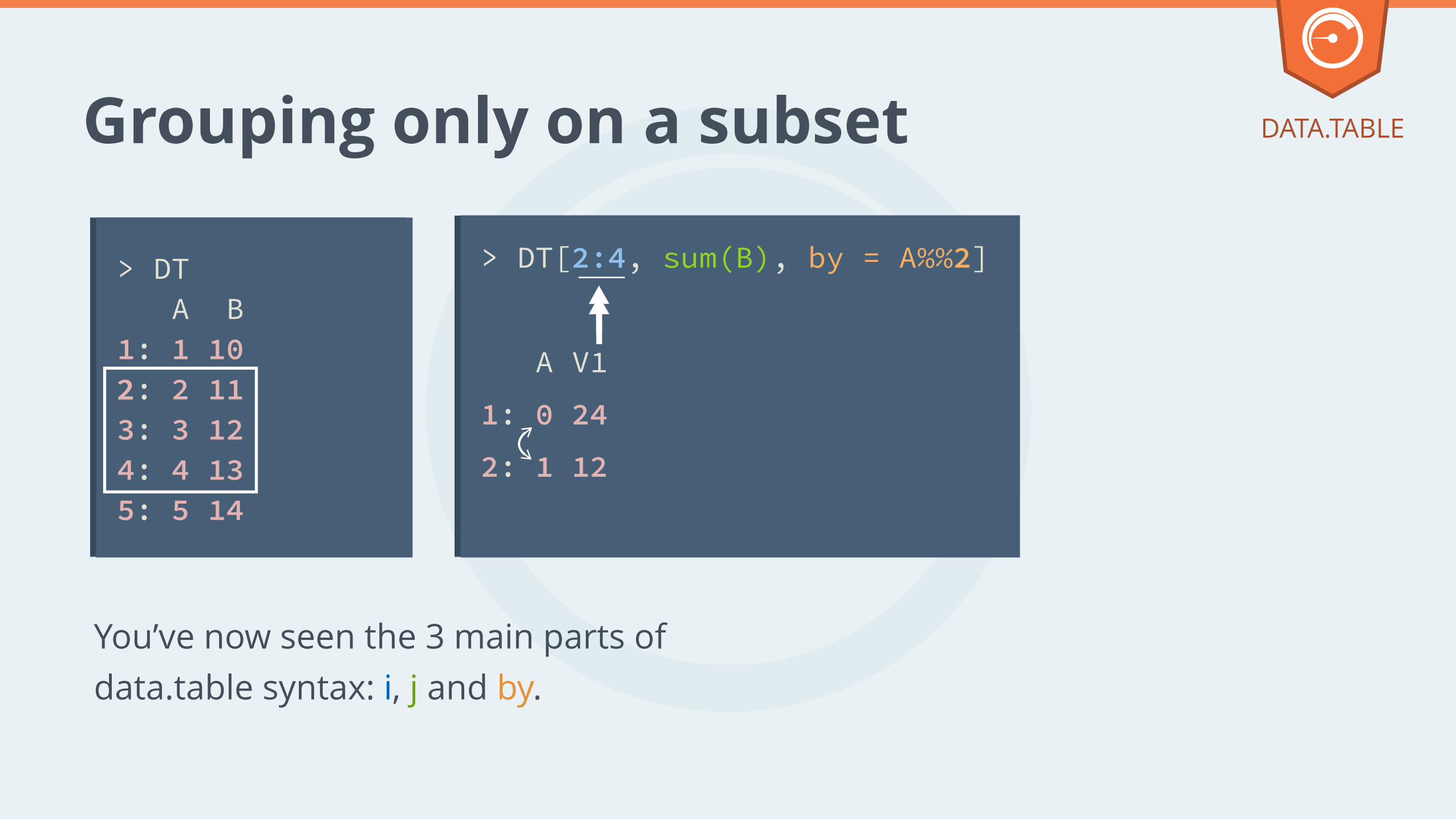
Grouping only on a subset

> DT A B 1: 1 10 2: 2 11 3: 3 12 4: 4 13 5: 5 14

> DT[2:4, sum(B), by = A%%2]

A V1

1: 0 24

2: 1 12

You’ve now seen the 3 main parts of data.table syntax: i, j and by.

DATA.TABLE

2

Let’s practice

DATA.TABLE