(data manipulation) 吳漢銘hmwu.idv.tw/web/r/b01-1-hmwu_r-datamanipulation.pdfdata manipulation,...
TRANSCRIPT

http://www.hmwu.idv.twhttp://www.hmwu.idv.tw http://www.hmwu.idv.tw
吳漢銘國立臺北大學 統計學系
http://www.hmwu.idv.tw
資料處理(Data Manipulation)
B01-1
http://www.hmwu.idv.twhttp://www.hmwu.idv.tw
本章大綱&學習目標 了解資料調處(處理) (Data Manipulation)的概念。
了解及運用表格處理函式: rbind {base}, cbind {base}, table {base}, xtabs {stats}, expand.table {epitools}, tabulate {base}, ftable {stats}, xtable {xtable}, stack {utils} .
了解及運用資料調處相關函式: aggregate {stats}, by {base}, cut {base}, with {base}, merge {base}, split {base}.
了解及運用apply系列於資料調處: apply, tapply, lapply, sapply, mapply, rapply.
了解及運用資料調處R套件: plyr, dplyr, tidyr, reshape2, data.table.
2/113

http://www.hmwu.idv.twhttp://www.hmwu.idv.tw
資料處理 (Data Manipulation) Some Terms:
Data Cleaning: https://en.wikipedia.org/wiki/Data_cleansing Data Integration: https://en.wikipedia.org/wiki/Data_integration Data Manipulation, Data Preprocessing Data Munging (data wrangling): munging can mean manipulating
raw data to achieve a final form. It can mean parsing or filtering data, or the many steps required for data recognition
Source: https://www.springboard.com/blog/data-science-career-paths-different-roles-industry/
國家教育研究院雙語詞彙
資料調處(data manipulation)
3/113

http://www.hmwu.idv.twhttp://www.hmwu.idv.tw
資料清理 (Data Cleaning) Data cleaning is one part of data quality. Aim at:
Accuracy (data is recorded correctly) Completeness (all relevant data is recorded) Uniqueness (no duplicated data record) Timeliness (the data is not old) Consistency (the data is coherent)
Data cleaning attempts to fill in missing values, smooth out noise while identifying outliers, and correct inconsistencies in the data.
Data cleaning is usually an iterative two-step process consisting of discrepancy detection and data transformation.
GIGO
4/113

http://www.hmwu.idv.twhttp://www.hmwu.idv.tw
Some R Functions for Data Manipulation R functions
aggregate{stats}: Compute Summary Statistics of Data Subsets
by{base}: Apply a Function to a Data Frame Split by Factors cut{base}: Convert Numeric to Factor with{base}: Evaluate an Expression in a Data Environment. merge{base}: Merge Two Data Frames split{base}: Divide into Groups and Reassemble
表格處理相關函式: rbind{base}, cbind{base}, table{base}, xtabs{stats}, expand.table{epitools}, tabulate{base}, ftable{stats}, xtable{xtable}, stack{utils}.
apply 系列: apply, tapply, sapply, lapply , rapply ,mapply.
5/113

http://www.hmwu.idv.twhttp://www.hmwu.idv.tw
tidyverse: Easily Install and Load 'Tidyverse' Packages
Core tidyverse packages
ggplot2: data visualisation.
dplyr: data manipulation.
tidyr: data tidying.
readr: data import.
purrr: functional programming.
tibble: tibbles, a modern re-imagining of data frames.
Other packages for data manipulation:
hms: times.
stringr: strings.
lubridate: date/times.
forcats: factors.
Data import:
DBI: databases.
haven: SPSS, SAS and Stata files.
httr: web apis.
jsonlite: JSON.
readxl: .xls and .xlsx files.
rvest: web scraping.
xml2: XML.
Modelling:
modelr: simple modelling within a pipeline
broom: turning models into tidy data
> install.packages("tidyverse")> library(tidyverse)
6/113

http://www.hmwu.idv.twhttp://www.hmwu.idv.tw
Tidy Data Tidy data is a standard way of mapping the meaning of a dataset to its
structure. A dataset is messy or tidy depending on how rows, columns and tables
are matched up with observations, variables and types. In tidy data: Each variable forms a column. Each observation forms a row. Each type of observational unit forms a table. (Each value is placed in its own cell)
Tidy data is particularly well suited for vectorised programming languages like R, because the layout ensures that values of different variables from the same observation are always paired.
https://cran.r-project.org/web/packages/tidyr/vignettes/tidy-data.html
7/113

http://www.hmwu.idv.twhttp://www.hmwu.idv.tw
Data Transformation with dplyrCheat Sheet by RStudio
https://github.com/rstudio/cheatsheets/raw/master/source/pdfs/data-transformation-cheatsheet.pdf
8/113

http://www.hmwu.idv.twhttp://www.hmwu.idv.tw
Data Transformation with dplyrCheat Sheet by RStudio
9/113

http://www.hmwu.idv.twhttp://www.hmwu.idv.tw
Data Wrangling with dplyr and tidyrCheat Sheet by RStudio
10/113

http://www.hmwu.idv.twhttp://www.hmwu.idv.tw
Data Wrangling with dplyr and tidyrCheat Sheet by RStudio
11/113

http://www.hmwu.idv.twhttp://www.hmwu.idv.tw
rbind and cbind> begin.experiment <- data.frame(name=c("A", "B", "C", "D", "E", "F"), + weights=c(270, 263, 294, 218, 305, 261))> middle.experiment <- data.frame(name=c("G", "H", "I"), + weights=c(169, 181, 201))> end.experiment <- data.frame(name=c("C", "D", "A", "H", "I"), + weights=c(107, 104, 104, 102, 100))> # merge the data for those who started and finished the experiment> (common <- intersect(begin.experiment$name, end.experiment$name))[1] "A" "C" "D"> (b.at <- is.element(begin.experiment$name, common))[1] TRUE FALSE TRUE TRUE FALSE FALSE> (e.at <- is.element(end.experiment$name, common))[1] TRUE TRUE TRUE FALSE FALSE> experiment <- rbind(cbind(begin.experiment[b.at,], time="begin"), + cbind(end.experiment[e.at,], time="end"))> experiment
name weights time1 A 270 begin3 C 294 begin4 D 218 begin11 C 107 end2 D 104 end31 A 104 end > tapply(experiment$weights, experiment$time, mean)
begin end 260.6667 105.0000
12/113
http://www.hmwu.idv.twhttp://www.hmwu.idv.tw
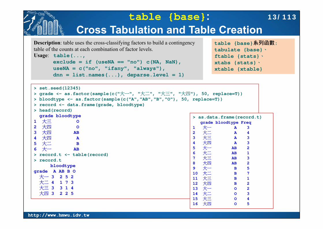
table {base}:Cross Tabulation and Table Creation
table {base}系列函數: tabulate {base}、ftable {stats}、xtabs {stats}、xtable {xtable}
Description: table uses the cross-classifying factors to build a contingency table of the counts at each combination of factor levels.Usage: table(...,
exclude = if (useNA == "no") c(NA, NaN),useNA = c("no", "ifany", "always"),dnn = list.names(...), deparse.level = 1)
> set.seed(12345)> grade <- as.factor(sample(c("大一", "大二", "大三", "大四"), 50, replace=T))> bloodtype <- as.factor(sample(c("A","AB","B","O"), 50, replace=T))> record <- data.frame(grade, bloodtype)> head(record)
grade bloodtype1 大三 O2 大四 O3 大四 AB4 大四 A5 大二 B6 大一 AB> record.t <- table(record)> record.t
bloodtypegrade A AB B O
大一 3 2 5 2大二 4 1 7 3大三 3 3 1 4大四 3 2 2 5
> as.data.frame(record.t)grade bloodtype Freq
1 大一 A 32 大二 A 43 大三 A 34 大四 A 35 大一 AB 26 大二 AB 17 大三 AB 38 大四 AB 29 大一 B 510 大二 B 711 大三 B 112 大四 B 213 大一 O 214 大二 O 315 大三 O 416 大四 O 5
13/113

http://www.hmwu.idv.twhttp://www.hmwu.idv.tw
table {base}:Cross Tabulation and Table Creation
> margin.table(record.t, 1)grade大一 大二 大三 大四
12 15 11 12 > margin.table(record.t, 2)bloodtypeA AB B O
13 8 15 14 > > colSums(record.t)A AB B O
13 8 15 14 > rowSums(record.t)大一 大二 大三 大四
12 15 11 12 >> colMeans(record.t)
A AB B O 3.25 2.00 3.75 3.50 > rowMeans(record.t)大一 大二 大三 大四3.00 3.75 2.75 3.00
> prop.table(record.t)bloodtype
grade A AB B O大一 0.06 0.04 0.10 0.04大二 0.08 0.02 0.14 0.06大三 0.06 0.06 0.02 0.08大四 0.06 0.04 0.04 0.10
> prop.table(record.t, margin=1) # row marginbloodtype
grade A AB B O大一 0.25000000 0.16666667 0.41666667 0.16666667大二 0.26666667 0.06666667 0.46666667 0.20000000大三 0.27272727 0.27272727 0.09090909 0.36363636大四 0.25000000 0.16666667 0.16666667 0.41666667
> prop.table(record.t, margin=2) # column marginbloodtype
grade A AB B O大一 0.23076923 0.25000000 0.33333333 0.14285714大二 0.30769231 0.12500000 0.46666667 0.21428571大三 0.23076923 0.37500000 0.06666667 0.28571429大四 0.23076923 0.25000000 0.13333333 0.35714286
> set.seed(12345)> (x <- sample(1:10, 5, replace=T))[1] 8 9 8 9 5> (y <- tabulate(x))[1] 0 0 0 0 1 0 0 2 2> names(y) <- as.character(1:max(x))> y1 2 3 4 5 6 7 8 9 0 0 0 0 1 0 0 2 2
tabulate {base}: Tabulation for VectorsDescription: tabulate takes the integer-valued vector bin and counts the number of times each integer occurs in it.Usage: tabulate(bin, nbins = max(1, bin, na.rm = TRUE))
14/113
http://www.hmwu.idv.twhttp://www.hmwu.idv.tw
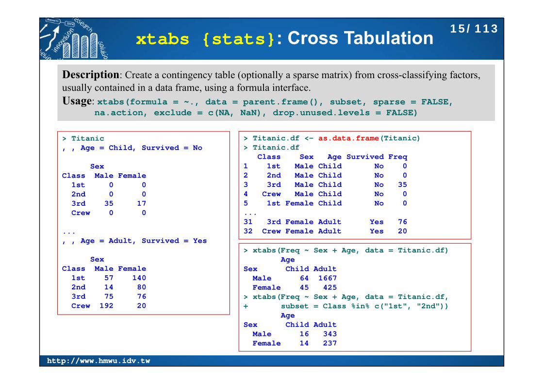
xtabs {stats}: Cross Tabulation
Description: Create a contingency table (optionally a sparse matrix) from cross-classifying factors, usually contained in a data frame, using a formula interface.Usage: xtabs(formula = ~., data = parent.frame(), subset, sparse = FALSE,
na.action, exclude = c(NA, NaN), drop.unused.levels = FALSE)
> Titanic, , Age = Child, Survived = No
SexClass Male Female
1st 0 02nd 0 03rd 35 17Crew 0 0
..., , Age = Adult, Survived = Yes
SexClass Male Female
1st 57 1402nd 14 803rd 75 76Crew 192 20
> Titanic.df <- as.data.frame(Titanic)> Titanic.df
Class Sex Age Survived Freq1 1st Male Child No 02 2nd Male Child No 03 3rd Male Child No 354 Crew Male Child No 05 1st Female Child No 0...31 3rd Female Adult Yes 7632 Crew Female Adult Yes 20
> xtabs(Freq ~ Sex + Age, data = Titanic.df)Age
Sex Child AdultMale 64 1667Female 45 425
> xtabs(Freq ~ Sex + Age, data = Titanic.df, + subset = Class %in% c("1st", "2nd"))
AgeSex Child Adult
Male 16 343Female 14 237
15/113

http://www.hmwu.idv.twhttp://www.hmwu.idv.tw
> sale <- read.table("itemsale.csv", sep=",", header=T)> sale
Item Date Count1 A 20170328 22 A 20170329 63 A 20170330 44 A 20170329 95 B 20170331 66 C 20170329 17 C 20170330 78 C 20170331 0> attach(sale)> tb <- xtabs(Freq ~ Item + Date)> rbind(cbind(tb, row.total=margin.table(tb, 1)), col.total=c(margin.table(tb, 2), sum(tb)))
20170328 20170329 20170330 20170331 row.totalA 2 15 4 0 21B 0 0 0 6 6C 0 1 7 0 8col.total 2 16 11 6 35> detach(sale)
樞紐分析
See also: http://www.cookbook-r.com/Manipulating_data/Converting_between_data_frames_and_contingency_tables/
16/113

http://www.hmwu.idv.twhttp://www.hmwu.idv.tw
expand.table {epitools}Expand contingency table into individual-level data set
> survey <- array(0, dim=c(3, 2, 1))> survey[,1,1] <- c(2, 0, 1) > survey[,2,1] <- c(3, 2, 4)> Satisfactory <- c("Good", "Fair", "Bad")> Sex <- c("Female", "Male")> Times <- c("First")> dimnames(survey) <- list(Satisfactory, Sex, Times)> names(dimnames(survey)) <- c("Satisfactory", "Sex", "Times")> survey, , Times = First
SexSatisfactory Female Male
Good 2 3Fair 0 2Bad 1 4
> (survey.ex <- expand.table(survey))Satisfactory Sex Times
1 Good Female First2 Good Female First3 Good Male First4 Good Male First5 Good Male First6 Fair Male First7 Fair Male First8 Bad Female First9 Bad Male First10 Bad Male First11 Bad Male First12 Bad Male First
expand.table {epitools}: Expand contingency table into individual-level data set• Usage: expand.table(x)• Arguments: x: table or array with
dimnames(x) and names(dimnames(x))
17/113

http://www.hmwu.idv.twhttp://www.hmwu.idv.tw
課堂練習: expand.table> data(HairEyeColor)> HairEyeColor, , Sex = Male
EyeHair Brown Blue Hazel Green
Black 32 11 10 3Brown 53 50 25 15Red 10 10 7 7Blond 3 30 5 8
, , Sex = Female
EyeHair Brown Blue Hazel Green
Black 36 9 5 2Brown 66 34 29 14Red 16 7 7 7Blond 4 64 5 8
> # Convert into individual-level data frame> HairEyeColor.ex <- expand.table(HairEyeColor) > HairEyeColor.ex
Hair Eye Sex1 Black Brown Male2 Black Brown Male 32 items3 Black Brown Male...589 Blond Green Female590 Blond Green Female591 Blond Green Female592 Blond Green Female
> # Convert into group-level data frame> as.data.frame(HairEyeColor)
Hair Eye Sex Freq1 Black Brown Male 322 Brown Brown Male 533 Red Brown Male 10...30 Brown Green Female 1431 Red Green Female 732 Blond Green Female 8
18/113
http://www.hmwu.idv.twhttp://www.hmwu.idv.tw
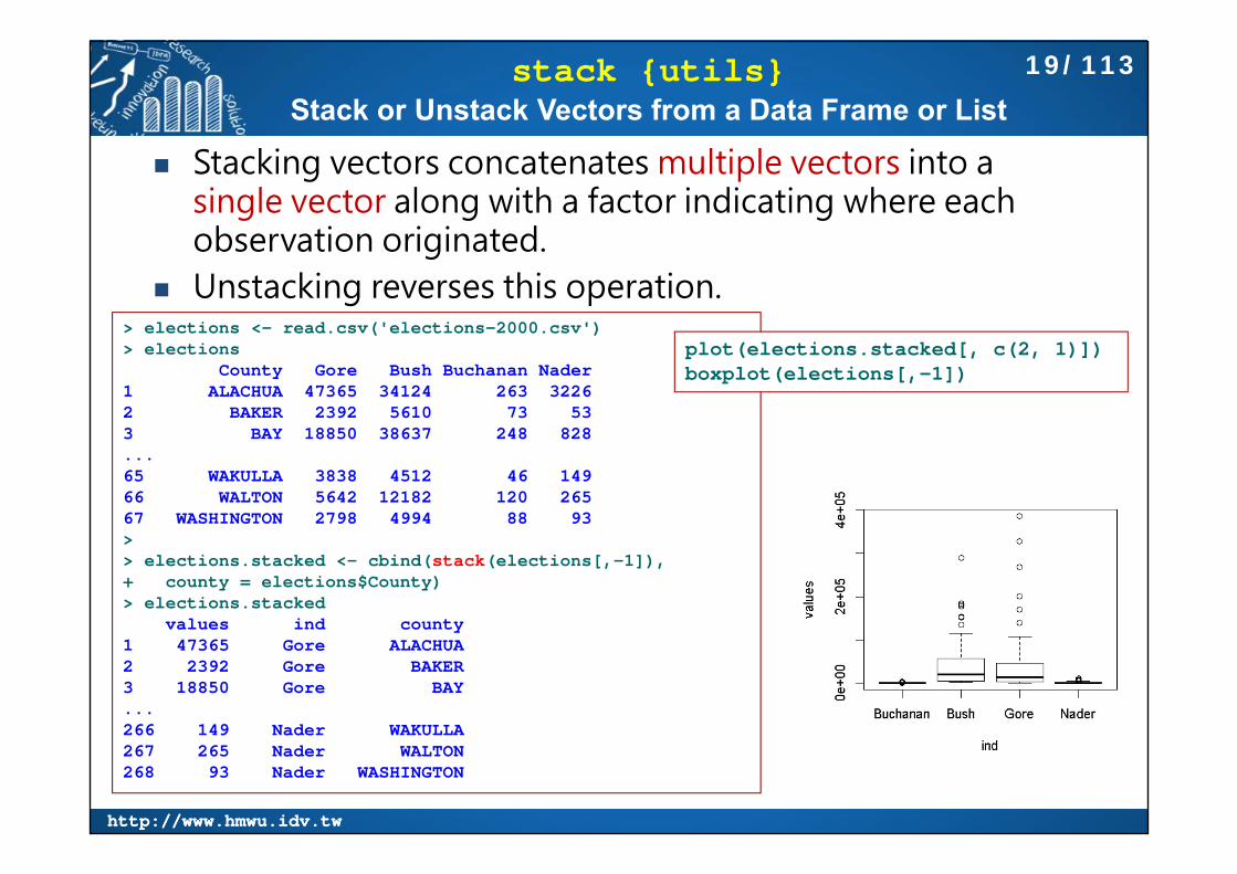
stack {utils}Stack or Unstack Vectors from a Data Frame or List
Stacking vectors concatenates multiple vectors into a single vector along with a factor indicating where each observation originated.
Unstacking reverses this operation.> elections <- read.csv('elections-2000.csv')> elections
County Gore Bush Buchanan Nader1 ALACHUA 47365 34124 263 32262 BAKER 2392 5610 73 533 BAY 18850 38637 248 828...65 WAKULLA 3838 4512 46 14966 WALTON 5642 12182 120 26567 WASHINGTON 2798 4994 88 93> > elections.stacked <- cbind(stack(elections[,-1]), + county = elections$County)> elections.stacked
values ind county1 47365 Gore ALACHUA2 2392 Gore BAKER3 18850 Gore BAY...266 149 Nader WAKULLA267 265 Nader WALTON268 93 Nader WASHINGTON
plot(elections.stacked[, c(2, 1)])boxplot(elections[,-1])
19/113

http://www.hmwu.idv.twhttp://www.hmwu.idv.tw
Stack Character Vectors> mydata <- data.frame(Area1=c("A", "B", "B", "C"), Area2=c("A", "D", "E", "B"))> rownames(mydata) <- paste("rater", 1:4, sep="-")> mydata
Area1 Area2rater-1 A Arater-2 B Drater-3 B Erater-4 C B> > stack(mydata)Error in stack.data.frame(mydata) : no vector columns were selected> mydata.stack <- stack(lapply(mydata, as.character))> colnames(mydata.stack) <- c("Rate", "Area")> mydata.stack
Rate Area1 A Area12 B Area13 B Area14 C Area15 A Area26 D Area27 E Area28 B Area2
20/113

http://www.hmwu.idv.twhttp://www.hmwu.idv.tw
aggregate {stats}: Compute Summary Statistics of Data Subsets
Usage: aggregate(x, by, FUN, ..., simplify = TRUE)
http://127.0.0.1:11812/library/datasets/html/state.html
> head(state.x77)Population Income Illiteracy Life Exp Murder HS Grad Frost Area
Alabama 3615 3624 2.1 69.05 15.1 41.3 20 50708Alaska 365 6315 1.5 69.31 11.3 66.7 152 566432Arizona 2212 4530 1.8 70.55 7.8 58.1 15 113417Arkansas 2110 3378 1.9 70.66 10.1 39.9 65 51945California 21198 5114 1.1 71.71 10.3 62.6 20 156361Colorado 2541 4884 0.7 72.06 6.8 63.9 166 103766> dim(state.x77)[1] 50 8> state.region[1] South West West South West [6] West Northeast South South South
...[46] South West South North Central West Levels: Northeast South North Central West> aggregate(state.x77, list(Region = state.region), mean)
Region Population Income Illiteracy Life Exp Murder HS Grad Frost Area1 Northeast 5495.111 4570.222 1.000000 71.26444 4.722222 53.96667 132.7778 18141.002 South 4208.125 4011.938 1.737500 69.70625 10.581250 44.34375 64.6250 54605.123 North Central 4803.000 4611.083 0.700000 71.76667 5.275000 54.51667 138.8333 62652.004 West 2915.308 4702.615 1.023077 71.23462 7.215385 62.00000 102.1538 134463.00
state{datasets}: US State Facts and Figures, Data sets related to the 50 states of the United States of America: state.abb, state.area, state.center, state.division, state.name, state.region, state.x77
tapply 可回傳list,aggregate僅能傳回向量、矩陣。
21/113

http://www.hmwu.idv.twhttp://www.hmwu.idv.tw
aggregate {stats}, Customized Statistics
> ## Compute the averages according to region and the occurrence of more> ## than 130 days of frost.> aggregate(state.x77,+ by = list(Region = state.region,+ Cold = state.x77[,"Frost"] > 130),+ FUN = function(x){round(mean(x), 2)})
Region Cold Population Income Illiteracy Life Exp Murder HS Grad Frost Area1 Northeast FALSE 8802.80 4780.40 1.18 71.13 5.58 52.06 110.60 21838.602 South FALSE 4208.12 4011.94 1.74 69.71 10.58 44.34 64.62 54605.123 North Central FALSE 7233.83 4633.33 0.78 70.96 8.28 53.37 120.00 56736.504 West FALSE 4582.57 4550.14 1.26 71.70 6.83 60.11 51.00 91863.715 Northeast TRUE 1360.50 4307.50 0.78 71.44 3.65 56.35 160.50 13519.006 North Central TRUE 2372.17 4588.83 0.62 72.58 2.27 55.67 157.67 68567.507 West TRUE 970.17 4880.50 0.75 70.69 7.67 64.20 161.83 184162.17
> aggregate(state.x77,+ by = list(Region = state.region,+ Cold = state.x77[,"Frost"] > 130),+ FUN = function(x){ round(sqrt(sum(x^2)), 2)})
Region Cold Population Income Illiteracy Life Exp Murder HS Grad Frost Area1 Northeast FALSE 23576.34 10707.22 2.66 159.05 14.13 116.74 250.13 66548.162 South FALSE 19980.44 16218.16 7.27 278.85 43.53 178.76 285.52 313220.523 North Central FALSE 19487.79 11367.76 1.94 173.82 21.00 130.97 294.40 144108.914 West FALSE 21791.15 12108.37 3.74 189.72 19.07 159.20 184.01 269467.525 Northeast TRUE 3407.56 8708.52 1.60 142.88 7.62 112.72 322.09 33868.126 North Central TRUE 6918.96 11260.58 1.53 177.78 5.73 136.59 388.46 169705.717 West TRUE 3013.82 12089.92 2.02 173.19 19.98 157.40 398.41 617310.24
22/113
http://www.hmwu.idv.twhttp://www.hmwu.idv.tw
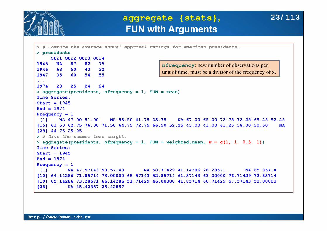
aggregate {stats}, FUN with Arguments
> # Compute the average annual approval ratings for American presidents.> presidents
Qtr1 Qtr2 Qtr3 Qtr41945 NA 87 82 751946 63 50 43 321947 35 60 54 55...1974 28 25 24 24> aggregate(presidents, nfrequency = 1, FUN = mean)Time Series:Start = 1945 End = 1974 Frequency = 1 [1] NA 47.00 51.00 NA 58.50 41.75 28.75 NA 67.00 65.00 72.75 72.25 65.25 52.25
[15] 61.50 62.75 76.00 71.50 64.75 72.75 66.50 52.25 45.00 41.00 61.25 58.00 50.50 NA[29] 44.75 25.25> # Give the summer less weight.> aggregate(presidents, nfrequency = 1, FUN = weighted.mean, w = c(1, 1, 0.5, 1))Time Series:Start = 1945 End = 1974 Frequency = 1 [1] NA 47.57143 50.57143 NA 58.71429 41.14286 28.28571 NA 65.85714
[10] 64.14286 71.85714 73.00000 65.57143 52.85714 61.57143 63.00000 76.71429 72.85714[19] 65.14286 73.28571 66.14286 51.71429 46.00000 41.85714 60.71429 57.57143 50.00000[28] NA 45.42857 25.42857
nfrequency: new number of observations per unit of time; must be a divisor of the frequency of x.
23/113

http://www.hmwu.idv.twhttp://www.hmwu.idv.tw
aggregate {stats},Example with Character Variables and NAs
> testDF <- data.frame(v1 = c(1,3,5,7,8,3,5,NA,4,5,7,9),+ v2 = c(11,33,55,77,88,33,55,NA,44,55,77,99))> by1 <- c("red", "blue", 1, 2, NA, "big", 1, 2, "red", 1, NA, 12)> by2 <- c("wet", "dry", 99, 95, NA, "damp", 95, 99, "red", 99, NA, NA)> aggregate(x = testDF, by = list(by1, by2), FUN = "mean")
Group.1 Group.2 v1 v21 1 95 5 552 2 95 7 773 1 99 5 554 2 99 NA NA5 big damp 3 336 blue dry 3 337 red red 4 448 red wet 1 11> # Treat NAs as a group> fby1 <- factor(by1, exclude = "")> fby2 <- factor(by2, exclude = "")> aggregate(x = testDF, by = list(fby1, fby2), FUN = "mean")
Group.1 Group.2 v1 v21 1 95 5.0 55.02 2 95 7.0 77.03 1 99 5.0 55.04 2 99 NA NA5 big damp 3.0 33.06 blue dry 3.0 33.07 red red 4.0 44.08 red wet 1.0 11.09 12 <NA> 9.0 99.010 <NA> <NA> 7.5 82.5
24/113

http://www.hmwu.idv.twhttp://www.hmwu.idv.tw
aggregate {stats},Formulas, one ~ one, one ~ many
> aggregate(weight ~ feed, data = chickwts, mean)
feed weight1 casein 323.58332 horsebean 160.20003 linseed 218.75004 meatmeal 276.90915 soybean 246.42866 sunflower 328.9167
> summary(chickwts)weight feed
Min. :108.0 casein :12 1st Qu.:204.5 horsebean:10 Median :258.0 linseed :12 Mean :261.3 meatmeal :11 3rd Qu.:323.5 soybean :14 Max. :423.0 sunflower:12
> aggregate(breaks ~ wool + tension, data = warpbreaks, mean)wool tension breaks
1 A L 44.555562 B L 28.222223 A M 24.000004 B M 28.777785 A H 24.555566 B H 18.77778
> summary(warpbreaks)breaks wool tension
Min. :10.00 A:27 L:18 1st Qu.:18.25 B:27 M:18 Median :26.00 H:18 Mean :28.15 3rd Qu.:34.00 Max. :70.00
25/113
http://www.hmwu.idv.twhttp://www.hmwu.idv.tw
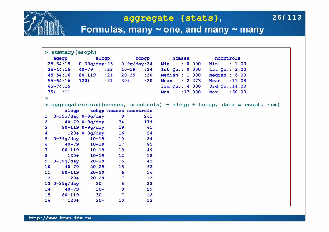
aggregate {stats},Formulas, many ~ one, and many ~ many
> summary(esoph)agegp alcgp tobgp ncases ncontrols
25-34:15 0-39g/day:23 0-9g/day:24 Min. : 0.000 Min. : 1.00 35-44:15 40-79 :23 10-19 :24 1st Qu.: 0.000 1st Qu.: 3.00 45-54:16 80-119 :21 20-29 :20 Median : 1.000 Median : 6.00 55-64:16 120+ :21 30+ :20 Mean : 2.273 Mean :11.08 65-74:15 3rd Qu.: 4.000 3rd Qu.:14.00 75+ :11 Max. :17.000 Max. :60.00 >> aggregate(cbind(ncases, ncontrols) ~ alcgp + tobgp, data = esoph, sum)
alcgp tobgp ncases ncontrols1 0-39g/day 0-9g/day 9 2612 40-79 0-9g/day 34 1793 80-119 0-9g/day 19 614 120+ 0-9g/day 16 245 0-39g/day 10-19 10 846 40-79 10-19 17 857 80-119 10-19 19 498 120+ 10-19 12 189 0-39g/day 20-29 5 4210 40-79 20-29 15 6211 80-119 20-29 6 1612 120+ 20-29 7 1213 0-39g/day 30+ 5 2814 40-79 30+ 9 2915 80-119 30+ 7 1216 120+ 30+ 10 13
26/113
http://www.hmwu.idv.twhttp://www.hmwu.idv.tw
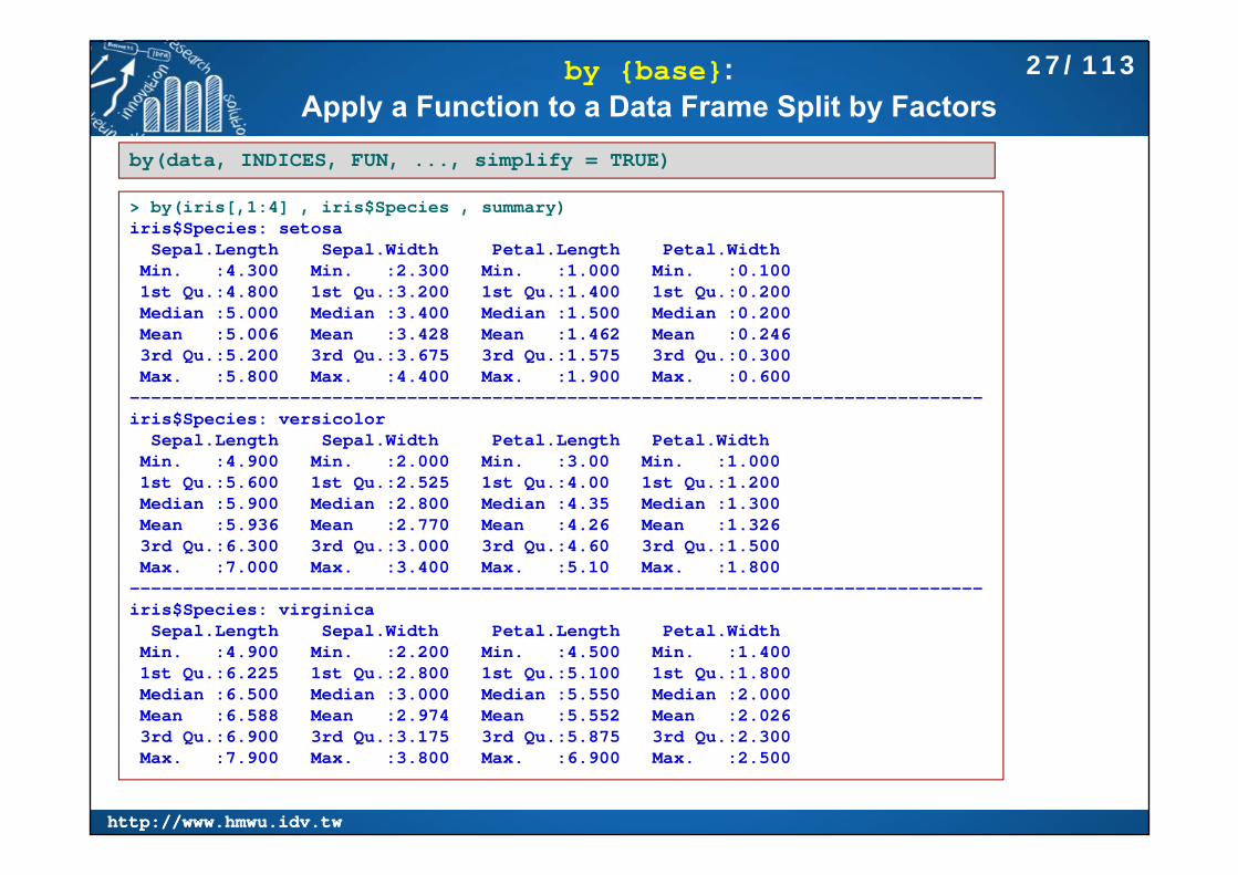
by {base}:Apply a Function to a Data Frame Split by Factors
by(data, INDICES, FUN, ..., simplify = TRUE)
> by(iris[,1:4] , iris$Species , summary)iris$Species: setosa
Sepal.Length Sepal.Width Petal.Length Petal.Width Min. :4.300 Min. :2.300 Min. :1.000 Min. :0.100 1st Qu.:4.800 1st Qu.:3.200 1st Qu.:1.400 1st Qu.:0.200 Median :5.000 Median :3.400 Median :1.500 Median :0.200 Mean :5.006 Mean :3.428 Mean :1.462 Mean :0.246 3rd Qu.:5.200 3rd Qu.:3.675 3rd Qu.:1.575 3rd Qu.:0.300 Max. :5.800 Max. :4.400 Max. :1.900 Max. :0.600
--------------------------------------------------------------------------------iris$Species: versicolor
Sepal.Length Sepal.Width Petal.Length Petal.Width Min. :4.900 Min. :2.000 Min. :3.00 Min. :1.000 1st Qu.:5.600 1st Qu.:2.525 1st Qu.:4.00 1st Qu.:1.200 Median :5.900 Median :2.800 Median :4.35 Median :1.300 Mean :5.936 Mean :2.770 Mean :4.26 Mean :1.326 3rd Qu.:6.300 3rd Qu.:3.000 3rd Qu.:4.60 3rd Qu.:1.500 Max. :7.000 Max. :3.400 Max. :5.10 Max. :1.800
--------------------------------------------------------------------------------iris$Species: virginica
Sepal.Length Sepal.Width Petal.Length Petal.Width Min. :4.900 Min. :2.200 Min. :4.500 Min. :1.400 1st Qu.:6.225 1st Qu.:2.800 1st Qu.:5.100 1st Qu.:1.800 Median :6.500 Median :3.000 Median :5.550 Median :2.000 Mean :6.588 Mean :2.974 Mean :5.552 Mean :2.026 3rd Qu.:6.900 3rd Qu.:3.175 3rd Qu.:5.875 3rd Qu.:2.300 Max. :7.900 Max. :3.800 Max. :6.900 Max. :2.500
27/113

http://www.hmwu.idv.twhttp://www.hmwu.idv.tw
by {base}, Example
> by(iris[,1:4] , iris$Species , mean)iris$Species: setosa[1] NA---------------------------------------------------iris$Species: versicolor[1] NA---------------------------------------------------iris$Species: virginica[1] NAWarning messages:1: In mean.default(data[x, , drop = FALSE], ...) :
argument is not numeric or logical: returning NA2: In mean.default(data[x, , drop = FALSE], ...) :
argument is not numeric or logical: returning NA3: In mean.default(data[x, , drop = FALSE], ...) :
argument is not numeric or logical: returning NA
The problem here is that the function you are applying doesn't work on a data frame. In effect you are calling something like this i.e. you are passing a data frame of 4 columns, containing the rows of the original where Species == "setosa".
> mean(iris[iris$Species == "setosa", 1:4])[1] NAWarning message:In mean.default(iris[iris$Species == "setosa", 1:4]) :
argument is not numeric or logical: returning NA
28/113

http://www.hmwu.idv.twhttp://www.hmwu.idv.tw
by {base}, Example
> by(iris[,1] , iris$Species , mean)iris$Species: setosa[1] 5.006-----------------------------------------------iris$Species: versicolor[1] 5.936-----------------------------------------------iris$Species: virginica[1] 6.588
For by() you need to do this variable by variable.
> by(iris[,1:4] , iris$Species , colMeans)iris$Species: setosaSepal.Length Sepal.Width Petal.Length Petal.Width
5.006 3.428 1.462 0.246 -----------------------------------------------------iris$Species: versicolorSepal.Length Sepal.Width Petal.Length Petal.Width
5.936 2.770 4.260 1.326 -----------------------------------------------------iris$Species: virginicaSepal.Length Sepal.Width Petal.Length Petal.Width
6.588 2.974 5.552 2.026
Use colMeans() instead of mean() as the FUN applied.
29/113

http://www.hmwu.idv.twhttp://www.hmwu.idv.tw
by {base}, Example
> varMean <- function(x, ...) sapply(x, mean, ...)> by(iris[, 1:4], iris$Species, varMean)iris$Species: setosaSepal.Length Sepal.Width Petal.Length Petal.Width
5.006 3.428 1.462 0.246 ----------------------------------------------------------------------------iris$Species: versicolorSepal.Length Sepal.Width Petal.Length Petal.Width
5.936 2.770 4.260 1.326 ----------------------------------------------------------------------------iris$Species: virginicaSepal.Length Sepal.Width Petal.Length Petal.Width
6.588 2.974 5.552 2.026
Write a wrapper, to sapply()
Use aggregate():> with(iris, aggregate(iris[,1:4], list(Species = iris$Species), FUN = mean))
Species Sepal.Length Sepal.Width Petal.Length Petal.Width1 setosa 5.006 3.428 1.462 0.2462 versicolor 5.936 2.770 4.260 1.3263 virginica 6.588 2.974 5.552 2.026
30/113

http://www.hmwu.idv.twhttp://www.hmwu.idv.tw
cut {base}: Convert Numeric to Factor cut{base} divides the range of x into intervals and codes the
values in x according to which interval they fall. The leftmost interval corresponds to level one, the next leftmost to level two and so on.
cut(x, breaks, labels = NULL,include.lowest = FALSE, right = TRUE, dig.lab = 3, ordered_result = FALSE, ...)
> x <- rnorm(50)> (x.cut1 <- cut(x, breaks = -5:5))[1] (-1,0] (-2,-1] (-2,-1] (-1,0] (-1,0] (-2,-1] (0,1] (0,1] (-1,0] (1,2] (0,1]
...[45] (1,2] (0,1] (-1,0] (-2,-1] (0,1] (0,1] Levels: (-5,-4] (-4,-3] (-3,-2] (-2,-1] (-1,0] (0,1] (1,2] (2,3] (3,4] (4,5]> table(x.cut1)x.cut1(-5,-4] (-4,-3] (-3,-2] (-2,-1] (-1,0] (0,1] (1,2] (2,3] (3,4] (4,5]
0 0 1 10 18 13 8 0 0 0 > (x.cut2 <- cut(x, breaks = -5:5, labels = FALSE))[1] 5 4 4 5 5 4 6 6 5 7 6 5 7 5 7 6 4 7 7 4 5 6 5 5 5 6 5 6 5 4 7 ...
[47] 5 4 6 6> table(x.cut2)x.cut23 4 5 6 7 1 10 18 13 8
> hist(x, breaks = -5:5, plot = FALSE)$counts[1] 0 0 1 10 18 13 8 0 0 0
31/113

http://www.hmwu.idv.twhttp://www.hmwu.idv.tw
cut {base} Examples> #the outer limits are moved away by 0.1% of the range> cut(0:10, 5)[1] (-0.01,2] (-0.01,2] (-0.01,2] (2,4] (2,4] (4,6] (4,6] (6,8] [9] (6,8] (8,10] (8,10]
Levels: (-0.01,2] (2,4] (4,6] (6,8] (8,10]> > age <- sample(0:80, 50, replace=T)> summary(age)
Min. 1st Qu. Median Mean 3rd Qu. Max. 1.00 21.00 35.00 38.16 52.75 80.00
> cut(age, 5)[1] (48.4,64.2] (16.8,32.6] (16.8,32.6] (48.4,64.2] (16.8,32.6] (32.6,48.4]
...[49] (16.8,32.6] (48.4,64.2] Levels: (0.921,16.8] (16.8,32.6] (32.6,48.4] (48.4,64.2] (64.2,80.1]> mygroup <- c(0, 15, 20, 50, 60, 80)> (x.cut <- cut(age, mygroup))[1] (50,60] (20,50] (15,20] (20,50] (20,50] (20,50] (15,20] (0,15] (0,15] (60,80]
...Levels: (0,15] (15,20] (20,50] (50,60] (60,80]> table(x.cut)x.cut(0,15] (15,20] (20,50] (50,60] (60,80]
7 5 22 8 8
Note: Instead of table(cut(x, br)), hist(x, br, plot = FALSE) is more efficient and less memory hungry. Instead of cut(*, labels = FALSE), findInterval() is more efficient.
32/113

http://www.hmwu.idv.twhttp://www.hmwu.idv.tw
with {base}:Evaluate an Expression in a Data Environment
> with(iris, {+ iris.lm <- lm(Sepal.Length ~ Petal.Length)+ summary(iris.lm)})
Call:lm(formula = Sepal.Length ~ Petal.Length)
Residuals:Min 1Q Median 3Q Max
-1.24675 -0.29657 -0.01515 0.27676 1.00269
Coefficients:Estimate Std. Error t value Pr(>|t|)
(Intercept) 4.30660 0.07839 54.94 <2e-16 ***Petal.Length 0.40892 0.01889 21.65 <2e-16 ***---Signif. codes: 0 ‘***’ 0.001 ‘**’ 0.01 ‘*’ 0.05 ‘.’ 0.1 ‘ ’ 1
Residual standard error: 0.4071 on 148 degrees of freedomMultiple R-squared: 0.76, Adjusted R-squared: 0.7583 F-statistic: 468.6 on 1 and 148 DF, p-value: < 2.2e-16
with(data, expr, ...)
People often use the attach()and detach() functions to set up "search paths" for variable names in R, but because this alters global state that's hard to keep track of, people recommend using with()instead, which sets up a temporary alteration to the search path for the duration of a single expression.
33/113

http://www.hmwu.idv.twhttp://www.hmwu.idv.tw
merge {base}: Merge Two Data Frames
Merge (adds variables to a dataset) two data frames horizontally by common columns or row names (key variables, either string or numeric). , or do other versions of database join operations.
https://stat.ethz.ch/R-manual/R-devel/library/base/html/merge.html
merge(x, y, by = intersect(names(x), names(y)),by.x = by, by.y = by, all = FALSE, all.x = all, all.y = all,sort = TRUE, suffixes = c(".x",".y"),incomparables = NULL, ...)
# merge two data frames by IDtotal <- merge(data.frame.A, data.frame.B, by="ID")
# merge two data frames by ID and Countrytotal <- merge(data.frame.A, data.frame.B, by=c("ID","Country"))
34/113
http://www.hmwu.idv.twhttp://www.hmwu.idv.tw
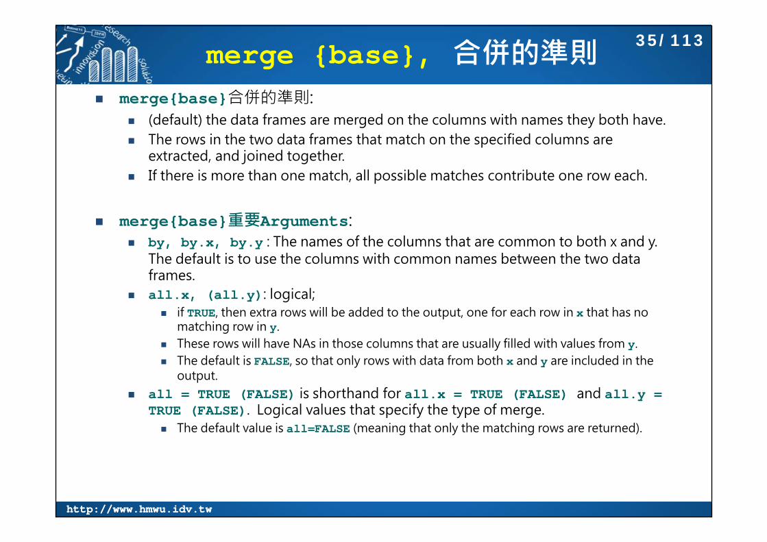
merge {base}, 合併的準則 merge{base}合併的準則:
(default) the data frames are merged on the columns with names they both have. The rows in the two data frames that match on the specified columns are
extracted, and joined together. If there is more than one match, all possible matches contribute one row each.
merge{base}重要Arguments: by, by.x, by.y : The names of the columns that are common to both x and y.
The default is to use the columns with common names between the two data frames.
all.x, (all.y): logical; if TRUE, then extra rows will be added to the output, one for each row in x that has no
matching row in y. These rows will have NAs in those columns that are usually filled with values from y. The default is FALSE, so that only rows with data from both x and y are included in the
output. all = TRUE (FALSE) is shorthand for all.x = TRUE (FALSE) and all.y =
TRUE (FALSE). Logical values that specify the type of merge. The default value is all=FALSE (meaning that only the matching rows are returned).
35/113
http://www.hmwu.idv.twhttp://www.hmwu.idv.tw
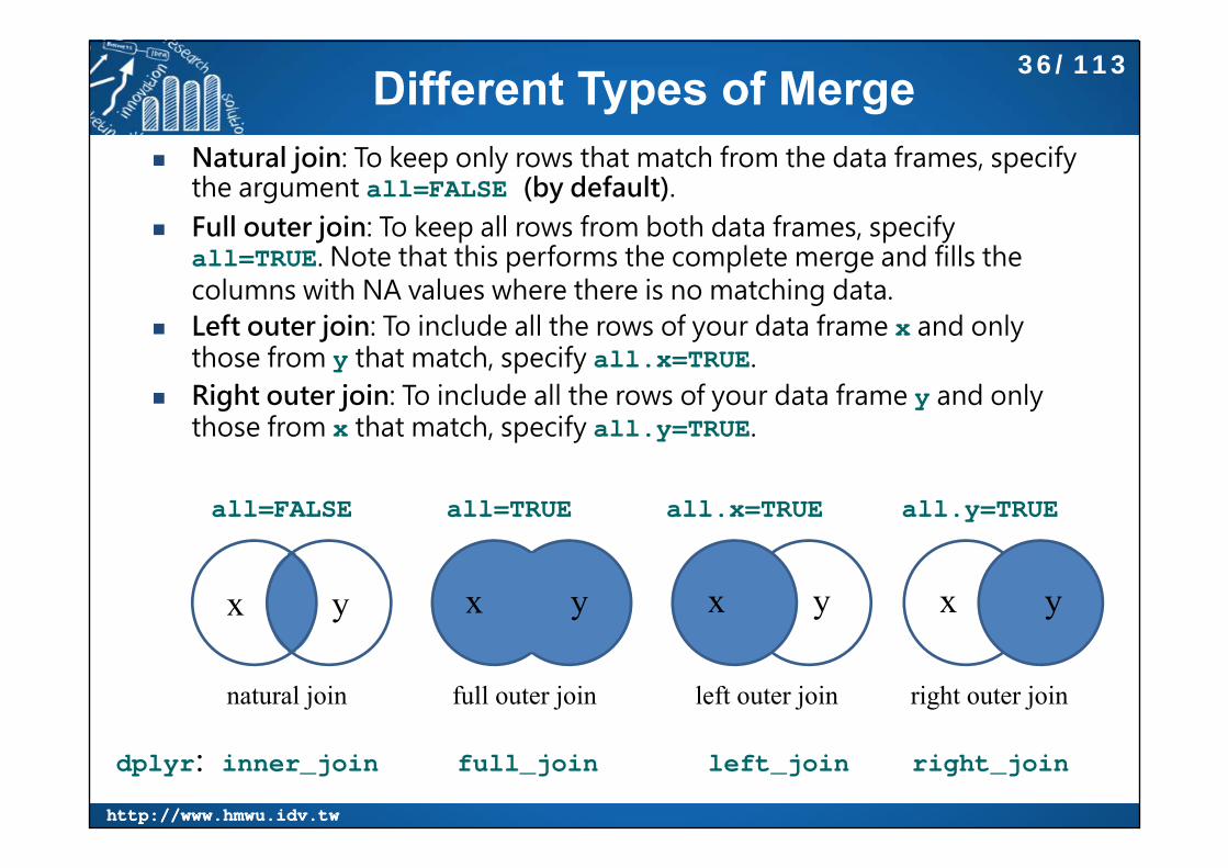
Different Types of Merge Natural join: To keep only rows that match from the data frames, specify
the argument all=FALSE (by default). Full outer join: To keep all rows from both data frames, specify
all=TRUE. Note that this performs the complete merge and fills the columns with NA values where there is no matching data.
Left outer join: To include all the rows of your data frame x and only those from y that match, specify all.x=TRUE.
Right outer join: To include all the rows of your data frame y and only those from x that match, specify all.y=TRUE.
natural join full outer join left outer join right outer join
all=FALSE all=TRUE all.x=TRUE all.y=TRUE
x y x y x y x y
dplyr: inner_join full_join left_join right_join
36/113

http://www.hmwu.idv.twhttp://www.hmwu.idv.tw
merge {base}, Example (1)
> authors <- data.frame(+ surname = I(c("Tukey", "Venables", "Tierney", "Ripley", "McNeil")),+ nationality = c("US", "Australia", "US", "UK", "Australia"),+ deceased = c("yes", rep("no", 4)))> books <- data.frame(+ name = I(c("Tukey", "Venables", "Tierney",+ "Ripley", "Ripley", "McNeil", "R Core")),+ title = c("Exploratory Data Analysis",+ "Modern Applied Statistics ...",+ "LISP-STAT",+ "Spatial Statistics", "Stochastic Simulation",+ "Interactive Data Analysis",+ "An Introduction to R"),+ other.author = c(NA, "Ripley", NA, NA, NA, NA, "Venables & Smith"))> authors
surname nationality deceased1 Tukey US yes2 Venables Australia no3 Tierney US no4 Ripley UK no5 McNeil Australia no> books
name title other.author1 Tukey Exploratory Data Analysis <NA>2 Venables Modern Applied Statistics ... Ripley3 Tierney LISP-STAT <NA>4 Ripley Spatial Statistics <NA>5 Ripley Stochastic Simulation <NA>6 McNeil Interactive Data Analysis <NA>7 R Core An Introduction to R Venables & Smith
https://stat.ethz.ch/R-manual/R-devel/library/base/html/merge.html
37/113
http://www.hmwu.idv.twhttp://www.hmwu.idv.tw
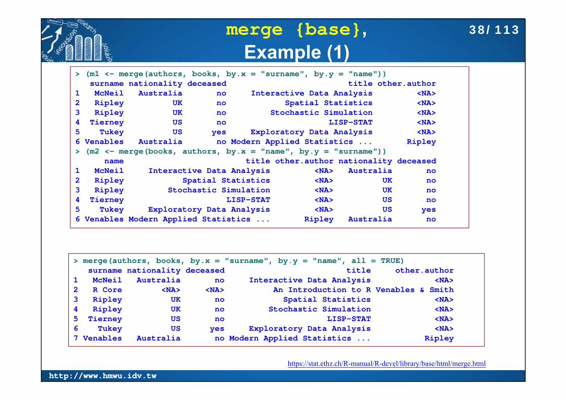
merge {base}, Example (1)
> (m1 <- merge(authors, books, by.x = "surname", by.y = "name"))surname nationality deceased title other.author
1 McNeil Australia no Interactive Data Analysis <NA>2 Ripley UK no Spatial Statistics <NA>3 Ripley UK no Stochastic Simulation <NA>4 Tierney US no LISP-STAT <NA>5 Tukey US yes Exploratory Data Analysis <NA>6 Venables Australia no Modern Applied Statistics ... Ripley> (m2 <- merge(books, authors, by.x = "name", by.y = "surname"))
name title other.author nationality deceased1 McNeil Interactive Data Analysis <NA> Australia no2 Ripley Spatial Statistics <NA> UK no3 Ripley Stochastic Simulation <NA> UK no4 Tierney LISP-STAT <NA> US no5 Tukey Exploratory Data Analysis <NA> US yes6 Venables Modern Applied Statistics ... Ripley Australia no
> merge(authors, books, by.x = "surname", by.y = "name", all = TRUE)surname nationality deceased title other.author
1 McNeil Australia no Interactive Data Analysis <NA>2 R Core <NA> <NA> An Introduction to R Venables & Smith3 Ripley UK no Spatial Statistics <NA>4 Ripley UK no Stochastic Simulation <NA>5 Tierney US no LISP-STAT <NA>6 Tukey US yes Exploratory Data Analysis <NA>7 Venables Australia no Modern Applied Statistics ... Ripley
https://stat.ethz.ch/R-manual/R-devel/library/base/html/merge.html
38/113

http://www.hmwu.idv.twhttp://www.hmwu.idv.tw
merge {base}, Example (2)
> (x <- data.frame(k1 = c(NA,NA,3,4,5), k2 = c(1,NA,NA,4,5), data = 1:5))k1 k2 data
1 NA 1 12 NA NA 23 3 NA 34 4 4 45 5 5 5> (y <- data.frame(k1 = c(NA,2,NA,4,5), k2 = c(NA,NA,3,4,5), data = 1:5))
k1 k2 data1 NA NA 12 2 NA 23 NA 3 34 4 4 45 5 5 5> merge(x, y, by = c("k1","k2")) # NA's match
k1 k2 data.x data.y1 4 4 4 42 5 5 5 53 NA NA 2 1> merge(x, y, by = "k1") # NA's match, so 6 rows
k1 k2.x data.x k2.y data.y1 4 4 4 4 42 5 5 5 5 53 NA 1 1 NA 14 NA 1 1 3 35 NA NA 2 NA 16 NA NA 2 3 3> merge(x, y, by = "k2", incomparables = NA) # 2 rows
k2 k1.x data.x k1.y data.y1 4 4 4 4 42 5 5 5 5
39/113

http://www.hmwu.idv.twhttp://www.hmwu.idv.tw
merge {base}, Example (3)
> stories <- read.table(header=TRUE, text='+ storyid title+ 1 lions+ 2 tigers+ 3 bears+ ')> data <- read.table(header=TRUE, text='+ subject storyid rating+ 1 1 6.7+ 1 2 4.5+ 1 3 3.7+ 2 2 3.3+ 2 3 4.1+ 2 1 5.2+ ')> > merge(stories, data, by="storyid")
storyid title subject rating1 1 lions 1 6.72 1 lions 2 5.23 2 tigers 1 4.54 2 tigers 2 3.35 3 bears 1 3.76 3 bears 2 4.1
> stories2 <- read.table(header=TRUE, text='+ id title+ 1 lions+ 2 tigers+ 3 bears+ ')> > merge(stories2, data, by.x="id", by.y="storyid")
id title subject rating1 1 lions 1 6.72 1 lions 2 5.23 2 tigers 1 4.54 2 tigers 2 3.35 3 bears 1 3.76 3 bears 2 4.1
http://www.cookbook-r.com/Manipulating_data/Merging_data_frames/
40/113

http://www.hmwu.idv.twhttp://www.hmwu.idv.tw
Merge on Multiple Columns> animals <- read.table(header=T, text='+ size type name+ small cat lynx+ big cat tiger+ small dog chihuahua+ big dog "great dane"+ ')> > observations <- read.table(header=T, text='+ number size type+ 1 big cat+ 2 small dog+ 3 small dog+ 4 big dog+ ')> > merge(observations, animals, c("size","type"))
size type number name1 big cat 1 tiger2 big dog 4 great dane3 small dog 2 chihuahua4 small dog 3 chihuahua
41/113

http://www.hmwu.idv.twhttp://www.hmwu.idv.tw
split {base}: Divide into Groups and Reassemble
split{base} divides the data in the vector x into the groups defined by f. The replacement forms replace values corresponding to such a division. unsplit{base} reverses the effect of split.
split(x, f, drop = FALSE, ...)split(x, f, drop = FALSE, ...) <- valueunsplit(value, f, drop = FALSE)
> n <- 10> edu <- factor(sample(1:4, n, replace=T))> score <- sample(0:100, n)> cbind(edu, score)
edu score[1,] 1 54[2,] 2 50[3,] 1 8[4,] 3 14[5,] 4 43[6,] 3 7[7,] 4 92[8,] 4 16[9,] 3 49
[10,] 4 51
> score.edu <- split(score, edu)> score.edu$`1`[1] 54 8
$`2`[1] 50
$`3`[1] 14 7 49
$`4`[1] 43 92 16 51
> unsplit(score.edu, edu)[1] 54 50 8 14 43 7 92 16 49 51
> sort(edu)[1] 1 1 2 3 3 3 4 4 4 4
Levels: 1 2 3 4> unsplit(score.edu, sort(edu))[1] 54 8 50 14 7 49 43 92 16 51
42/113
http://www.hmwu.idv.twhttp://www.hmwu.idv.tw
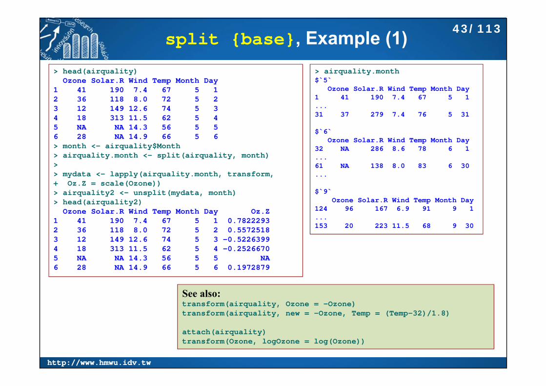
split {base}, Example (1)> head(airquality)
Ozone Solar.R Wind Temp Month Day1 41 190 7.4 67 5 12 36 118 8.0 72 5 23 12 149 12.6 74 5 34 18 313 11.5 62 5 45 NA NA 14.3 56 5 56 28 NA 14.9 66 5 6> month <- airquality$Month> airquality.month <- split(airquality, month)>> mydata <- lapply(airquality.month, transform, + Oz.Z = scale(Ozone))> airquality2 <- unsplit(mydata, month)> head(airquality2)
Ozone Solar.R Wind Temp Month Day Oz.Z1 41 190 7.4 67 5 1 0.78222932 36 118 8.0 72 5 2 0.55725183 12 149 12.6 74 5 3 -0.52263994 18 313 11.5 62 5 4 -0.25266705 NA NA 14.3 56 5 5 NA6 28 NA 14.9 66 5 6 0.1972879
See also:transform(airquality, Ozone = -Ozone)transform(airquality, new = -Ozone, Temp = (Temp-32)/1.8)
attach(airquality)transform(Ozone, logOzone = log(Ozone))
> airquality.month$`5`
Ozone Solar.R Wind Temp Month Day1 41 190 7.4 67 5 1...31 37 279 7.4 76 5 31
$`6`Ozone Solar.R Wind Temp Month Day
32 NA 286 8.6 78 6 1...61 NA 138 8.0 83 6 30...
$`9`Ozone Solar.R Wind Temp Month Day
124 96 167 6.9 91 9 1...153 20 223 11.5 68 9 30
43/113

http://www.hmwu.idv.twhttp://www.hmwu.idv.tw
split{base}, Example (2)
> # Split a matrix into a list by columns> mat <- cbind(x = 1:10, y = (-4:5)^2)> cbind(mat, col(mat))
x y [1,] 1 16 1 2[2,] 2 9 1 2[3,] 3 4 1 2[4,] 4 1 1 2[5,] 5 0 1 2[6,] 6 1 1 2[7,] 7 4 1 2[8,] 8 9 1 2[9,] 9 16 1 2
[10,] 10 25 1 2> split(mat, col(mat))$`1`[1] 1 2 3 4 5 6 7 8 9 10
$`2`[1] 16 9 4 1 0 1 4 9 16 25
> split(1:10, 1:2)$`1`[1] 1 3 5 7 9
$`2`[1] 2 4 6 8 10
44/113

http://www.hmwu.idv.twhttp://www.hmwu.idv.tw
apply {base}:Apply Functions Over Array Margins
> (x <- matrix(1:24, nrow=4))[,1] [,2] [,3] [,4] [,5] [,6]
[1,] 1 5 9 13 17 21[2,] 2 6 10 14 18 22[3,] 3 7 11 15 19 23[4,] 4 8 12 16 20 24> > #1: rows, 2:columns> apply(x, 1, sum) [1] 66 72 78 84> apply(x, 2, sum)[1] 10 26 42 58 74 90> > #apply function to the individual elements> > apply(x, 1, sqrt)
[,1] [,2] [,3] [,4][1,] 1.000000 1.414214 1.732051 2.000000[2,] 2.236068 2.449490 2.645751 2.828427[3,] 3.000000 3.162278 3.316625 3.464102[4,] 3.605551 3.741657 3.872983 4.000000[5,] 4.123106 4.242641 4.358899 4.472136[6,] 4.582576 4.690416 4.795832 4.898979> apply(x, 2, sqrt)
[,1] [,2] [,3] [,4] [,5] [,6][1,] 1.000000 2.236068 3.000000 3.605551 4.123106 4.582576[2,] 1.414214 2.449490 3.162278 3.741657 4.242641 4.690416[3,] 1.732051 2.645751 3.316625 3.872983 4.358899 4.795832[4,] 2.000000 2.828427 3.464102 4.000000 4.472136 4.898979
Description: Returns a vector or array or list of values obtained by applying a function to margins of an array or matrix.Usage: apply(X, MARGIN, FUN, ...)
apply系列: tapply、lapply、sapply、mapply、rapply
45/113
http://www.hmwu.idv.twhttp://www.hmwu.idv.tw
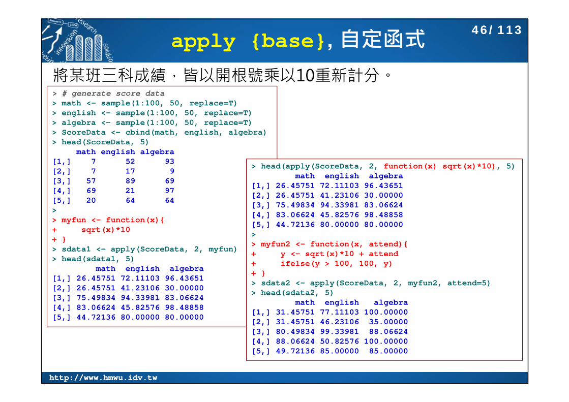
apply {base}, 自定函式
> # generate score data> math <- sample(1:100, 50, replace=T)> english <- sample(1:100, 50, replace=T)> algebra <- sample(1:100, 50, replace=T)> ScoreData <- cbind(math, english, algebra)> head(ScoreData, 5)
math english algebra[1,] 7 52 93[2,] 7 17 9[3,] 57 89 69[4,] 69 21 97[5,] 20 64 64> > myfun <- function(x){+ sqrt(x)*10+ }> sdata1 <- apply(ScoreData, 2, myfun)> head(sdata1, 5)
math english algebra[1,] 26.45751 72.11103 96.43651[2,] 26.45751 41.23106 30.00000[3,] 75.49834 94.33981 83.06624[4,] 83.06624 45.82576 98.48858[5,] 44.72136 80.00000 80.00000
> head(apply(ScoreData, 2, function(x) sqrt(x)*10), 5)math english algebra
[1,] 26.45751 72.11103 96.43651[2,] 26.45751 41.23106 30.00000[3,] 75.49834 94.33981 83.06624[4,] 83.06624 45.82576 98.48858[5,] 44.72136 80.00000 80.00000> > myfun2 <- function(x, attend){+ y <- sqrt(x)*10 + attend+ ifelse(y > 100, 100, y)+ }> sdata2 <- apply(ScoreData, 2, myfun2, attend=5)> head(sdata2, 5)
math english algebra[1,] 31.45751 77.11103 100.00000[2,] 31.45751 46.23106 35.00000[3,] 80.49834 99.33981 88.06624[4,] 88.06624 50.82576 100.00000[5,] 49.72136 85.00000 85.00000
將某班三科成績,皆以開根號乘以10重新計分。
46/113
http://www.hmwu.idv.twhttp://www.hmwu.idv.tw
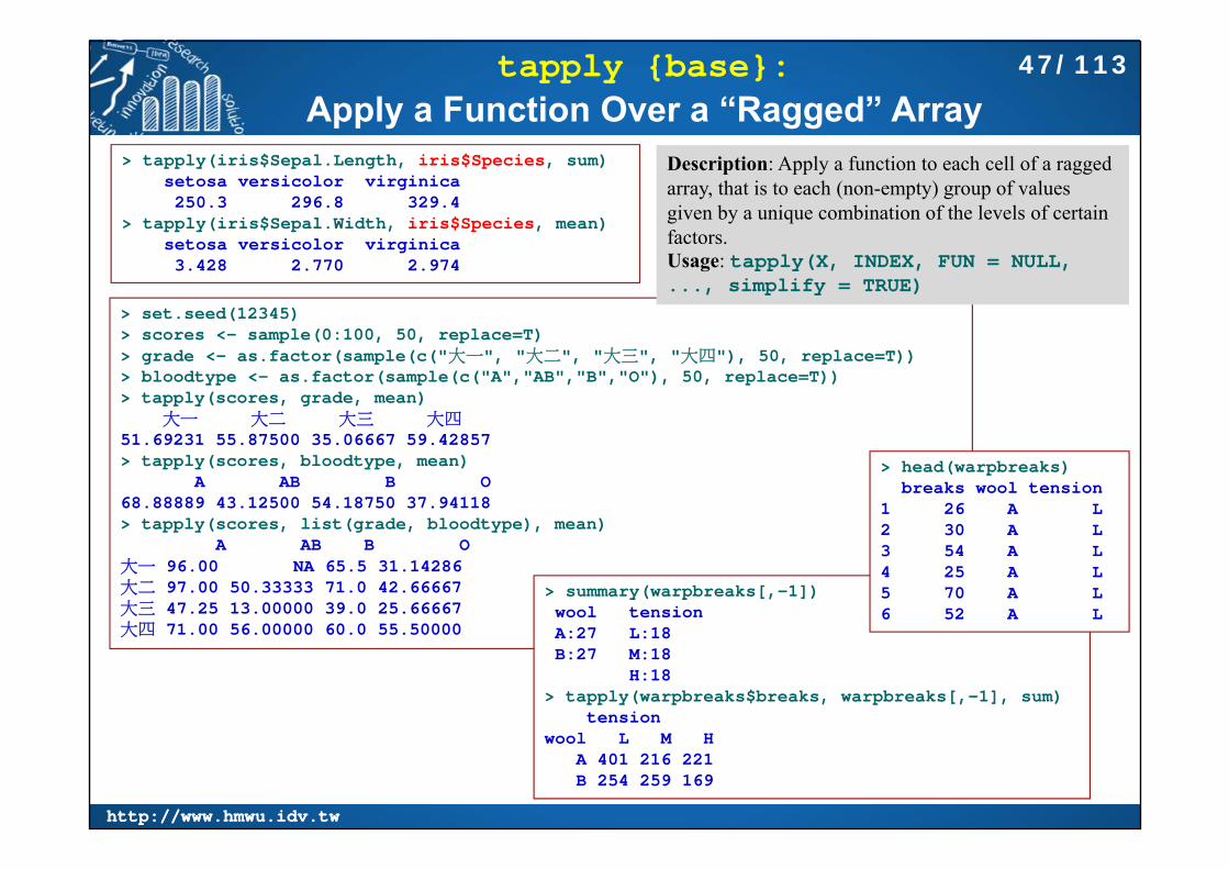
tapply {base}:Apply a Function Over a “Ragged” Array
> tapply(iris$Sepal.Length, iris$Species, sum)setosa versicolor virginica 250.3 296.8 329.4
> tapply(iris$Sepal.Width, iris$Species, mean)setosa versicolor virginica 3.428 2.770 2.974
> set.seed(12345)> scores <- sample(0:100, 50, replace=T)> grade <- as.factor(sample(c("大一", "大二", "大三", "大四"), 50, replace=T))> bloodtype <- as.factor(sample(c("A","AB","B","O"), 50, replace=T))> tapply(scores, grade, mean)
大一 大二 大三 大四51.69231 55.87500 35.06667 59.42857 > tapply(scores, bloodtype, mean)
A AB B O 68.88889 43.12500 54.18750 37.94118 > tapply(scores, list(grade, bloodtype), mean)
A AB B O大一 96.00 NA 65.5 31.14286大二 97.00 50.33333 71.0 42.66667大三 47.25 13.00000 39.0 25.66667大四 71.00 56.00000 60.0 55.50000
> summary(warpbreaks[,-1])wool tensionA:27 L:18 B:27 M:18
H:18 > tapply(warpbreaks$breaks, warpbreaks[,-1], sum)
tensionwool L M H
A 401 216 221B 254 259 169
Description: Apply a function to each cell of a ragged array, that is to each (non-empty) group of values given by a unique combination of the levels of certain factors.Usage: tapply(X, INDEX, FUN = NULL, ..., simplify = TRUE)
> head(warpbreaks)breaks wool tension
1 26 A L2 30 A L3 54 A L4 25 A L5 70 A L6 52 A L
47/113

http://www.hmwu.idv.twhttp://www.hmwu.idv.tw
tapply {base}:Apply a Function Over a “Ragged” Array
> n <- 20> (my.factor <- factor(rep(1:3, length = n), levels = 1:5))[1] 1 2 3 1 2 3 1 2 3 1 2 3 1 2 3 1 2 3 1 2
Levels: 1 2 3 4 5> table(my.factor)my.factor1 2 3 4 5 7 7 6 0 0 > tapply(1:n, my.factor, sum)1 2 3 4 5
70 77 63 NA NA > presidentsQtr1 Qtr2 Qtr3 Qtr4
1945 NA 87 82 751946 63 50 43 32...1974 28 25 24 24> class(presidents)[1] "ts"> # gives the positions in the cycle of each observation. > cycle(presidents) Qtr1 Qtr2 Qtr3 Qtr41945 1 2 3 41946 1 2 3 4...1974 1 2 3 4> tapply(presidents, cycle(presidents), mean, na.rm=T)
1 2 3 4 58.44828 56.43333 57.22222 53.07143
> tapply(1:n, my.factor, range)$`1`[1] 1 19$`2`[1] 2 20$`3`[1] 3 18$`4`NULL$`5`NULL
48/113

http://www.hmwu.idv.twhttp://www.hmwu.idv.tw
lapply {base}:Apply a Function over a List or Vector
lapply returns a list of the same length as X, each element of which is the result of applying FUN to the corresponding element of X.
> a <- c("a", "b", "c", "d")> b <- c(1, 2, 3, 4, 4, 3, 2, 1)> c <- c(T, T, F)> list.object <- list(a,b,c)> my.la1 <- lapply(list.object, length)> my.la1[[1]][1] 4
[[2]][1] 8
[[3]][1] 3> my.la2 <- lapply(list.object, class)> my.la2[[1]][1] "character"
[[2]][1] "numeric"
[[3]][1] "logical"
> x <- list(a = 1:10, beta = exp(-3:3), logic = c(TRUE,FALSE,FALSE,TRUE))> lapply(x, mean) # return list$a[1] 5.5
$beta[1] 4.535125
$logic[1] 0.5> # median and quartiles for each list element> lapply(x, quantile, probs = 1:3/4)$a25% 50% 75%
3.25 5.50 7.75
$beta25% 50% 75%
0.2516074 1.0000000 5.0536690
$logic25% 50% 75% 0.0 0.5 1.0
49/113
http://www.hmwu.idv.twhttp://www.hmwu.idv.tw
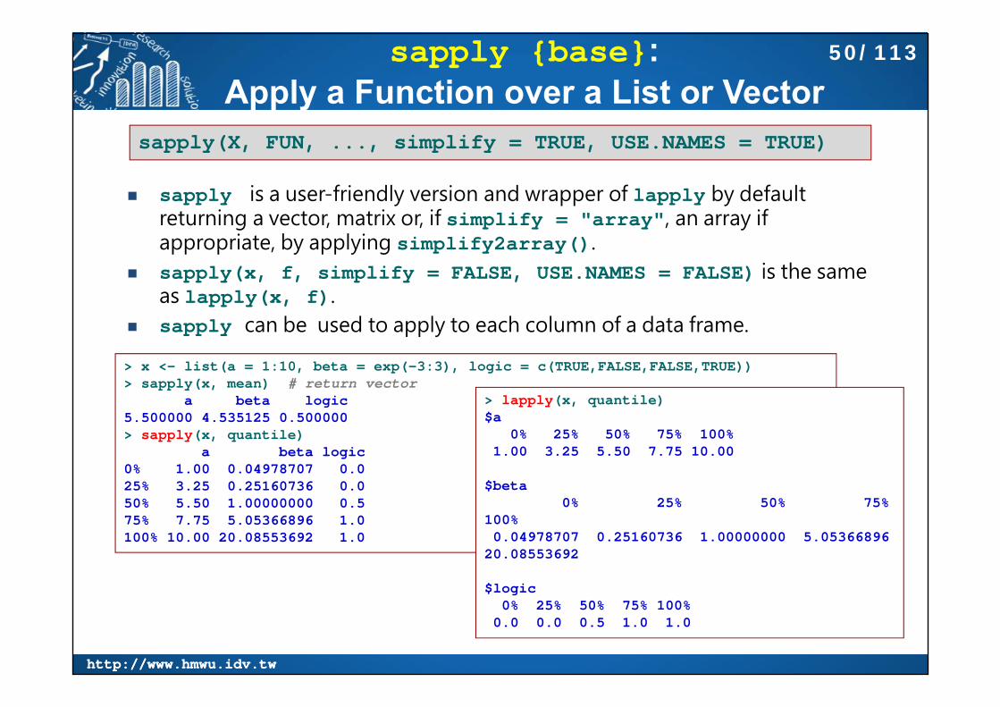
sapply {base}: Apply a Function over a List or Vector
sapply is a user-friendly version and wrapper of lapply by default returning a vector, matrix or, if simplify = "array", an array if appropriate, by applying simplify2array().
sapply(x, f, simplify = FALSE, USE.NAMES = FALSE) is the same as lapply(x, f).
sapply can be used to apply to each column of a data frame.
sapply(X, FUN, ..., simplify = TRUE, USE.NAMES = TRUE)
> x <- list(a = 1:10, beta = exp(-3:3), logic = c(TRUE,FALSE,FALSE,TRUE))> sapply(x, mean) # return vector
a beta logic 5.500000 4.535125 0.500000 > sapply(x, quantile)
a beta logic0% 1.00 0.04978707 0.025% 3.25 0.25160736 0.050% 5.50 1.00000000 0.575% 7.75 5.05366896 1.0100% 10.00 20.08553692 1.0
> lapply(x, quantile)$a
0% 25% 50% 75% 100% 1.00 3.25 5.50 7.75 10.00
$beta0% 25% 50% 75%
100% 0.04978707 0.25160736 1.00000000 5.05366896
20.08553692
$logic0% 25% 50% 75% 100%
0.0 0.0 0.5 1.0 1.0
50/113
http://www.hmwu.idv.twhttp://www.hmwu.idv.tw
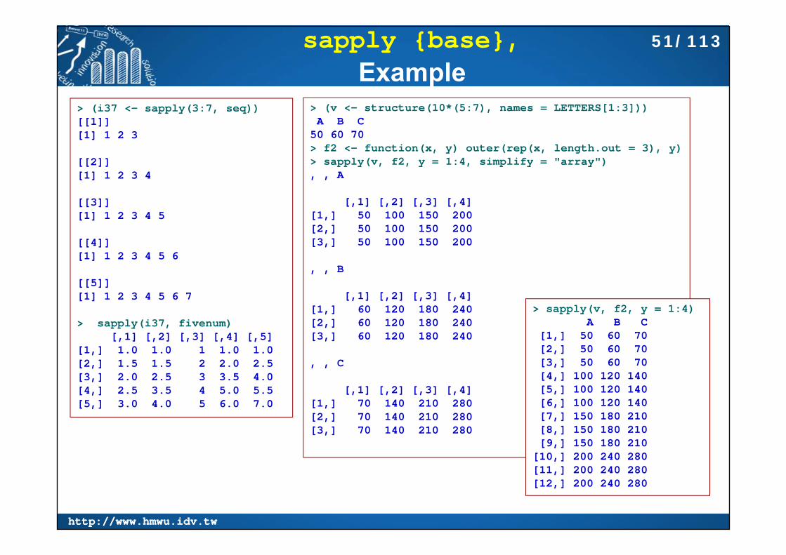
sapply {base},Example
> (i37 <- sapply(3:7, seq))[[1]][1] 1 2 3
[[2]][1] 1 2 3 4
[[3]][1] 1 2 3 4 5
[[4]][1] 1 2 3 4 5 6
[[5]][1] 1 2 3 4 5 6 7
> sapply(i37, fivenum)[,1] [,2] [,3] [,4] [,5]
[1,] 1.0 1.0 1 1.0 1.0[2,] 1.5 1.5 2 2.0 2.5[3,] 2.0 2.5 3 3.5 4.0[4,] 2.5 3.5 4 5.0 5.5[5,] 3.0 4.0 5 6.0 7.0
> (v <- structure(10*(5:7), names = LETTERS[1:3]))A B C
50 60 70 > f2 <- function(x, y) outer(rep(x, length.out = 3), y)> sapply(v, f2, y = 1:4, simplify = "array"), , A
[,1] [,2] [,3] [,4][1,] 50 100 150 200[2,] 50 100 150 200[3,] 50 100 150 200
, , B
[,1] [,2] [,3] [,4][1,] 60 120 180 240[2,] 60 120 180 240[3,] 60 120 180 240
, , C
[,1] [,2] [,3] [,4][1,] 70 140 210 280[2,] 70 140 210 280[3,] 70 140 210 280
> sapply(v, f2, y = 1:4)A B C
[1,] 50 60 70[2,] 50 60 70[3,] 50 60 70[4,] 100 120 140[5,] 100 120 140[6,] 100 120 140[7,] 150 180 210[8,] 150 180 210[9,] 150 180 210
[10,] 200 240 280[11,] 200 240 280[12,] 200 240 280
51/113

http://www.hmwu.idv.twhttp://www.hmwu.idv.tw
sapply {base},[[ 運算子
"[[" 跟 "[" 是 operator (運算子)> my.list <- list(name=c("George", "John", "Tom"),+ wife=c("Mary", "Sue", "Nico"), + no.children=c(3, 2, 0), + child.ages=list(c(4,7,9), c(2, 5), NA))> > # 取出某一家庭的資訊> my.list[[1]][1][1] "George"> my.list[[2]][1][1] "Mary"> my.list[[3]][1][1] 3> my.list[[4]][1][[1]][1] 4 7 9
> my.list[[1:4]][1] # ErrorError in my.list[[1:4]] : 遞迴索引在 2 層失敗
> George.family <- sapply(my.list,"[[", 1)> George.family$name[1] "George"
$wife[1] "Mary"
$no.children[1] 3
$child.ages[1] 4 7 9
52/113
http://www.hmwu.idv.twhttp://www.hmwu.idv.tw
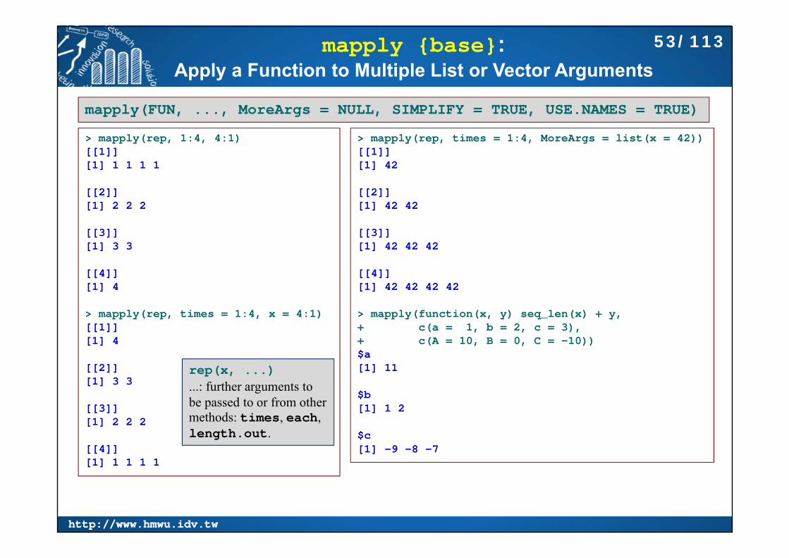
mapply {base}: Apply a Function to Multiple List or Vector Arguments
mapply(FUN, ..., MoreArgs = NULL, SIMPLIFY = TRUE, USE.NAMES = TRUE)
> mapply(rep, 1:4, 4:1)[[1]][1] 1 1 1 1
[[2]][1] 2 2 2
[[3]][1] 3 3
[[4]][1] 4
> mapply(rep, times = 1:4, x = 4:1)[[1]][1] 4
[[2]][1] 3 3
[[3]][1] 2 2 2
[[4]][1] 1 1 1 1
> mapply(rep, times = 1:4, MoreArgs = list(x = 42))[[1]][1] 42
[[2]][1] 42 42
[[3]][1] 42 42 42
[[4]][1] 42 42 42 42
> mapply(function(x, y) seq_len(x) + y,+ c(a = 1, b = 2, c = 3), + c(A = 10, B = 0, C = -10))$a[1] 11
$b[1] 1 2
$c[1] -9 -8 -7
rep(x, ...)...: further arguments to be passed to or from other methods: times, each, length.out.
53/113
http://www.hmwu.idv.twhttp://www.hmwu.idv.tw
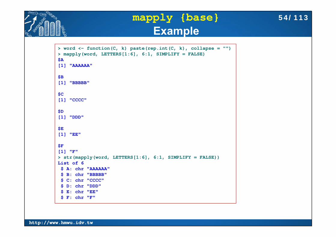
mapply {base}Example
> word <- function(C, k) paste(rep.int(C, k), collapse = "")> mapply(word, LETTERS[1:6], 6:1, SIMPLIFY = FALSE)$A[1] "AAAAAA"
$B[1] "BBBBB"
$C[1] "CCCC"
$D[1] "DDD"
$E[1] "EE"
$F[1] "F"> str(mapply(word, LETTERS[1:6], 6:1, SIMPLIFY = FALSE))List of 6$ A: chr "AAAAAA"$ B: chr "BBBBB"$ C: chr "CCCC"$ D: chr "DDD"$ E: chr "EE"$ F: chr "F"
54/113

http://www.hmwu.idv.twhttp://www.hmwu.idv.tw
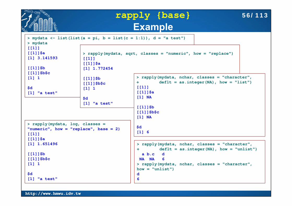
rapply {base}: Recursively Apply a Function to a List
rapply is a recursive version of lapply. Arguments:
object: A list. f: A function of a single argument. classes: A character vector of class names, or "ANY" to match any
class. deflt: The default result (not used if how = "replace"). how: A character string partially matching the three possibilities
given. If how = "replace", each element of the list which is not itself a list and has
a class included in classes is replaced by the result of applying f to the element.
If how = "list" or how = "unlist", the list is copied, all non-list elements which have a class included in classes are replaced by the result of applying f to the element and all others are replaced by deflt.
if how = "unlist", unlist(recursive = TRUE) is called on the result.
rapply(object, f, classes = "ANY", deflt = NULL,how = c("unlist", "replace", "list"), ...)
55/113
http://www.hmwu.idv.twhttp://www.hmwu.idv.tw
rapply {base}Example
> rapply(mydata, nchar, classes = "character",+ deflt = as.integer(NA), how = "unlist")
a b.c d NA NA 6
> rapply(mydata, nchar, classes = "character", how = "unlist")d 6
> rapply(mydata, log, classes = "numeric", how = "replace", base = 2)[[1]][[1]]$a[1] 1.651496
[[1]]$b[[1]]$b$c[1] 1
$d[1] "a test"
> mydata <- list(list(a = pi, b = list(c = 1:1)), d = "a test")> mydata[[1]][[1]]$a[1] 3.141593
[[1]]$b[[1]]$b$c[1] 1
$d[1] "a test"
> rapply(mydata, sqrt, classes = "numeric", how = "replace")[[1]][[1]]$a[1] 1.772454
[[1]]$b[[1]]$b$c[1] 1
$d[1] "a test"
> rapply(mydata, nchar, classes = "character",+ deflt = as.integer(NA), how = "list")[[1]][[1]]$a[1] NA
[[1]]$b[[1]]$b$c[1] NA
$d[1] 6
56/113
http://www.hmwu.idv.twhttp://www.hmwu.idv.tw
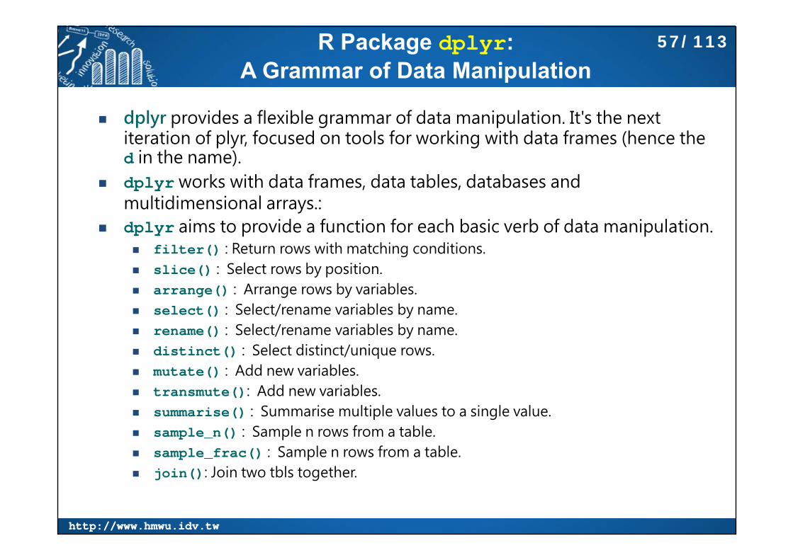
R Package dplyr: A Grammar of Data Manipulation
dplyr provides a flexible grammar of data manipulation. It's the next iteration of plyr, focused on tools for working with data frames (hence the d in the name).
dplyr works with data frames, data tables, databases and multidimensional arrays.:
dplyr aims to provide a function for each basic verb of data manipulation. filter() : Return rows with matching conditions. slice() : Select rows by position. arrange() : Arrange rows by variables. select() : Select/rename variables by name. rename() : Select/rename variables by name. distinct() : Select distinct/unique rows. mutate() : Add new variables. transmute(): Add new variables. summarise() : Summarise multiple values to a single value. sample_n() : Sample n rows from a table. sample_frac() : Sample n rows from a table. join(): Join two tbls together.
57/113

http://www.hmwu.idv.twhttp://www.hmwu.idv.tw
R Package dplyr
> browseVignettes(package = "dplyr")
中文介紹: CELESTIAL, Introduction to dplyrhttp://chingchuan-chen.github.io/r/2015/07/03/dplyr
Pipe operator: %>%dplyr provides the %>% operator. x %>% f(y)turns into f(x, y) so you can use it to rewrite multiple operations that you can read left-to-right, top-to-bottom.
> x <- rnorm(10)> x %>% max> # is the same thing as:> max(x)
58/113

http://www.hmwu.idv.twhttp://www.hmwu.idv.tw
Flights Data flights {nycflights13}: On-time data for all flights that departed NYC in 2013. Variables:
year,month,day: Date of departure dep_time,arr_time: Departure and arrival times, local tz. dep_delay,arr_delay: Departure and arrival delays, in minutes.
Negative times represent early departures/arrivals. hour,minute: Time of departure broken in to hour and minutes carrier: Two letter carrier abbreviation. See airlines to get name tailnum: Plane tail number flight: Flight number origin,dest: Origin and destination. See airports for additional metadata. air_time: Amount of time spent in the air distance: Distance flown
https://cran.rstudio.com/web/packages/dplyr/vignettes/introduction.html
> library(nycflights13)> dim(flights)[1] 336776 16> head(flights, 4)year month day dep_time dep_delay arr_time arr_delay carrier
1 2013 1 1 517 2 830 11 UA2 2013 1 1 533 4 850 20 UA3 2013 1 1 542 2 923 33 AA4 2013 1 1 544 -1 1004 -18 B6tailnum flight origin dest air_time distance hour minute
1 N14228 1545 EWR IAH 227 1400 5 172 N24211 1714 LGA IAH 227 1416 5 333 N619AA 1141 JFK MIA 160 1089 5 424 N804JB 725 JFK BQN 183 1576 5 44
NOTE: dealing with large data, it’s worthwhile to convert them to a tbl_df: this is a wrapper around a data frame that won’t accidentally print a lot of data to the screen.
59/113

http://www.hmwu.idv.twhttp://www.hmwu.idv.tw
filter {dplyr}: Return Rows with Matching Conditions
> library(dplyr)> filter(flights, month == 1, day == 1) #same as filter(flights, month == 1 & day == 1)Source: local data frame [842 x 16]
year month day dep_time dep_delay arr_time arr_delay carrier tailnum flight origin dest air_time distance hour minute(int) (int) (int) (int) (dbl) (int) (dbl) (chr) (chr) (int) (chr) (chr) (dbl) (dbl) (dbl) (dbl)
1 2013 1 1 517 2 830 11 UA N14228 1545 EWR IAH 227 1400 5 172 2013 1 1 533 4 850 20 UA N24211 1714 LGA IAH 227 1416 5 33.. ... ... ... ... ... ... ... ... ... ... ... ... ... ... ... ...
> flights[flights$month == 1 & flights$day == 1, ]Source: local data frame [842 x 16]
year month day dep_time dep_delay arr_time arr_delay carrier tailnum flight origin dest air_time distance hour minute(int) (int) (int) (int) (dbl) (int) (dbl) (chr) (chr) (int) (chr) (chr) (dbl) (dbl) (dbl) (dbl)
1 2013 1 1 517 2 830 11 UA N14228 1545 EWR IAH 227 1400 5 172 2013 1 1 533 4 850 20 UA N24211 1714 LGA IAH 227 1416 5 33.. ... ... ... ... ... ... ... ... ... ... ... ... ... ... ... ...
> table(flights$carrier)9E AA AS B6 DL EV F9 FL HA MQ OO UA US VX WN
YV 18460 32729 714 54635 48110 54173 685 3260 342 26397 32 58665 20536 5162 12275 601 > filter(flights, carrier %in% c("OO", "YV"))Source: local data frame [633 x 16]
year month day dep_time dep_delay arr_time arr_delay carrier tailnum flight origin dest air_time ...(int) (int) (int) (int) (dbl) (int) (dbl) (chr) (chr) (int) (chr) (chr) (dbl) ...
1 2013 1 3 1428 -7 1539 -20 YV N509MJ 3750 LGA IAD 47 ...2 2013 1 3 1551 -11 1659 -23 YV N508MJ 3771 LGA IAD 47 ...3 2013 1 4 1430 -5 1546 -13 YV N511MJ 3750 LGA IAD 55 ..... ... ... ... ... ... ... ... ... ... ... ... ... ... ...
60/113

http://www.hmwu.idv.twhttp://www.hmwu.idv.tw
subset {base}: Subsetting Vectors, Matrices and Data Frames
filter() works similarly to subset() except that you can give it any number of filtering conditions.
> subset(flights, dep_delay < 0, select = c(carrier, distance))Source: local data frame [183,575 x 2]
carrier distance(chr) (dbl)
1 B6 15762 DL 762.. ... ...> subset(flights, origin == "JFK", select = -year)Source: local data frame [111,279 x 15]
month day dep_time dep_delay arr_time arr_delay carrier tailnum flight origin dest air_time distance hour minute(int) (int) (int) (dbl) (int) (dbl) (chr) (chr) (int) (chr) (chr) (dbl) (dbl) (dbl) (dbl)
1 1 1 542 2 923 33 AA N619AA 1141 JFK MIA 160 1089 5 422 1 1 544 -1 1004 -18 B6 N804JB 725 JFK BQN 183 1576 5 44.. ... ... ... ... ... ... ... ... ... ... ... ... ... ... ...
> airquality.sub2 <- subset(airquality, Temp > 80, select = c(Ozone, Temp))> head(airquality.sub2, 3)
Ozone Temp29 45 8135 NA 8436 NA 85
> airquality.sub3 <- subset(airquality, select = Ozone:Wind)> head(airquality.sub3, 3)
Ozone Solar.R Wind1 41 190 7.42 36 118 8.03 12 149 12.6
> airquality.sub1 <- subset(airquality, Day == 1, select = -Temp)> head(airquality.sub1, 3)
Ozone Solar.R Wind Month Day1 41 190 7.4 5 132 NA 286 8.6 6 162 135 269 4.1 7 1
> head(airquality, 3)Ozone Solar.R Wind Temp Month Day
1 41 190 7.4 67 5 12 36 118 8.0 72 5 23 12 149 12.6 74 5 3
61/113
http://www.hmwu.idv.twhttp://www.hmwu.idv.tw
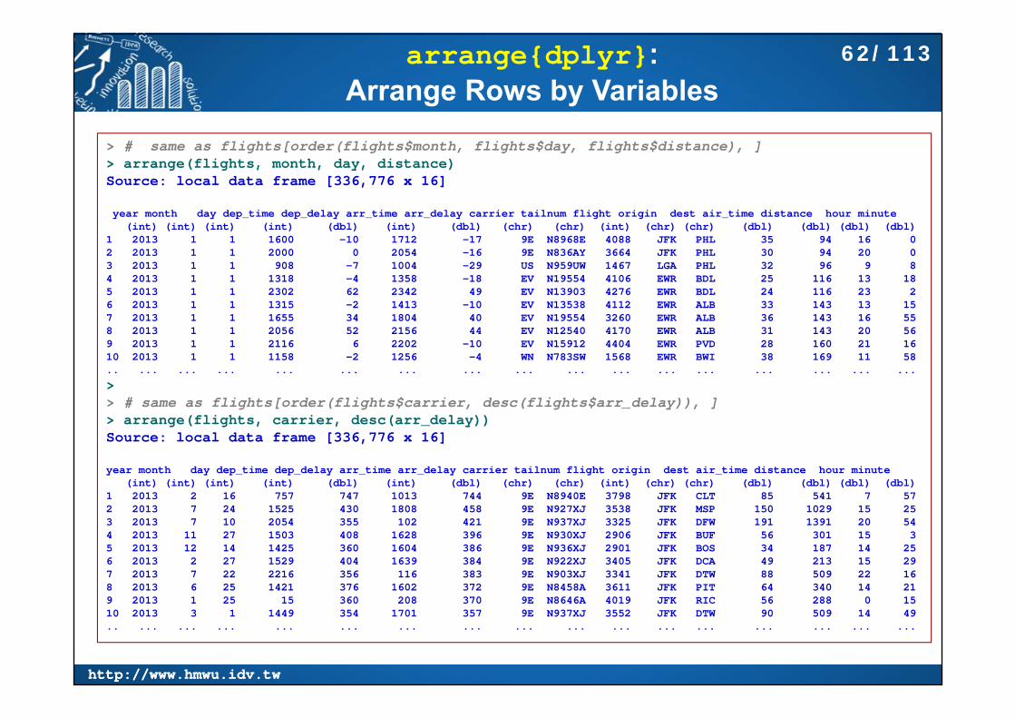
arrange{dplyr}: Arrange Rows by Variables
> # same as flights[order(flights$month, flights$day, flights$distance), ]> arrange(flights, month, day, distance) Source: local data frame [336,776 x 16]
year month day dep_time dep_delay arr_time arr_delay carrier tailnum flight origin dest air_time distance hour minute(int) (int) (int) (int) (dbl) (int) (dbl) (chr) (chr) (int) (chr) (chr) (dbl) (dbl) (dbl) (dbl)
1 2013 1 1 1600 -10 1712 -17 9E N8968E 4088 JFK PHL 35 94 16 02 2013 1 1 2000 0 2054 -16 9E N836AY 3664 JFK PHL 30 94 20 03 2013 1 1 908 -7 1004 -29 US N959UW 1467 LGA PHL 32 96 9 84 2013 1 1 1318 -4 1358 -18 EV N19554 4106 EWR BDL 25 116 13 185 2013 1 1 2302 62 2342 49 EV N13903 4276 EWR BDL 24 116 23 26 2013 1 1 1315 -2 1413 -10 EV N13538 4112 EWR ALB 33 143 13 157 2013 1 1 1655 34 1804 40 EV N19554 3260 EWR ALB 36 143 16 558 2013 1 1 2056 52 2156 44 EV N12540 4170 EWR ALB 31 143 20 569 2013 1 1 2116 6 2202 -10 EV N15912 4404 EWR PVD 28 160 21 1610 2013 1 1 1158 -2 1256 -4 WN N783SW 1568 EWR BWI 38 169 11 58.. ... ... ... ... ... ... ... ... ... ... ... ... ... ... ... ...
>> # same as flights[order(flights$carrier, desc(flights$arr_delay)), ]> arrange(flights, carrier, desc(arr_delay))Source: local data frame [336,776 x 16]
year month day dep_time dep_delay arr_time arr_delay carrier tailnum flight origin dest air_time distance hour minute(int) (int) (int) (int) (dbl) (int) (dbl) (chr) (chr) (int) (chr) (chr) (dbl) (dbl) (dbl) (dbl)
1 2013 2 16 757 747 1013 744 9E N8940E 3798 JFK CLT 85 541 7 572 2013 7 24 1525 430 1808 458 9E N927XJ 3538 JFK MSP 150 1029 15 253 2013 7 10 2054 355 102 421 9E N937XJ 3325 JFK DFW 191 1391 20 544 2013 11 27 1503 408 1628 396 9E N930XJ 2906 JFK BUF 56 301 15 35 2013 12 14 1425 360 1604 386 9E N936XJ 2901 JFK BOS 34 187 14 256 2013 2 27 1529 404 1639 384 9E N922XJ 3405 JFK DCA 49 213 15 297 2013 7 22 2216 356 116 383 9E N903XJ 3341 JFK DTW 88 509 22 168 2013 6 25 1421 376 1602 372 9E N8458A 3611 JFK PIT 64 340 14 219 2013 1 25 15 360 208 370 9E N8646A 4019 JFK RIC 56 288 0 1510 2013 3 1 1449 354 1701 357 9E N937XJ 3552 JFK DTW 90 509 14 49.. ... ... ... ... ... ... ... ... ... ... ... ... ... ... ... ...
62/113

http://www.hmwu.idv.twhttp://www.hmwu.idv.tw
select{dplyr}: Select/Rename Variables by Name
There are a number of special functions that only work inside select starts_with(x, ignore.case = TRUE): names starts with x ends_with(x, ignore.case = TRUE): names ends in x contains(x, ignore.case = TRUE): selects all variables whose name
contains x matches(x, ignore.case = TRUE): selects all variables whose name
matches the regular expression x num_range("x", 1:5, width = 2): selects all variables (numerically)
from x01 to x05. one_of("x", "y", "z"): selects variables provided in a character
vector. everything(): selects all variables. To drop variables, use -. You can rename variables with named
arguments.
This function works similarly to the select argument in subset{base}.
63/113

http://www.hmwu.idv.twhttp://www.hmwu.idv.tw
select{dplyr}Example (1)
> select(flights, origin, carrier, distance) #Select columns by nameSource: local data frame [336,776 x 3]
origin carrier distance(chr) (chr) (dbl)
1 EWR UA 14002 LGA UA 14163 JFK AA 1089.. ... ... ...> select(flights, dep_time:arr_delay) #Select all columns between variables (inclusive)Source: local data frame [336,776 x 4]
dep_time dep_delay arr_time arr_delay(int) (dbl) (int) (dbl)
1 517 2 830 112 533 4 850 203 542 2 923 33.. ... ... ... ...> select(flights, -(year:day)) # Select all columns except those from year to day (inclusive)Source: local data frame [336,776 x 13]
dep_time dep_delay arr_time arr_delay carrier tailnum flight origin dest air_time distance hour minute(int) (dbl) (int) (dbl) (chr) (chr) (int) (chr) (chr) (dbl) (dbl) (dbl) (dbl)
1 517 2 830 11 UA N14228 1545 EWR IAH 227 1400 5 172 533 4 850 20 UA N24211 1714 LGA IAH 227 1416 5 333 542 2 923 33 AA N619AA 1141 JFK MIA 160 1089 5 42.. ... ... ... ... ... ... ... ... ... ... ... ... ...
64/113

http://www.hmwu.idv.twhttp://www.hmwu.idv.tw
select{dplyr}, Example (1)
> select(flights, tail_num = tailnum) #drops all the variables not explicitly mentionedSource: local data frame [336,776 x 1]
tail_num(chr)
1 N142282 N24211.. ...> > rename(flights, DepTime = dep_time, DepDelay = dep_delay)Source: local data frame [336,776 x 16]
year month day DepTime DepDelay arr_time arr_delay carrier tailnum flight origin dest air_time distance ..(int) (int) (int) (int) (dbl) (int) (dbl) (chr) (chr) (int) (chr) (chr) (dbl) (dbl) ..
1 2013 1 1 517 2 830 11 UA N14228 1545 EWR IAH 227 1400 ..2 2013 1 1 533 4 850 20 UA N24211 1714 LGA IAH 227 1416 .... ... ... ... ... ... ... ... ... ... ... ... ... ... ... ..
65/113
http://www.hmwu.idv.twhttp://www.hmwu.idv.tw
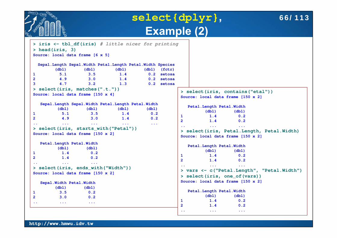
select{dplyr}, Example (2)
> iris <- tbl_df(iris) # little nicer for printing> head(iris, 3)Source: local data frame [6 x 5]
Sepal.Length Sepal.Width Petal.Length Petal.Width Species(dbl) (dbl) (dbl) (dbl) (fctr)
1 5.1 3.5 1.4 0.2 setosa2 4.9 3.0 1.4 0.2 setosa3 4.7 3.2 1.3 0.2 setosa> select(iris, matches(".t."))Source: local data frame [150 x 4]
Sepal.Length Sepal.Width Petal.Length Petal.Width(dbl) (dbl) (dbl) (dbl)
1 5.1 3.5 1.4 0.22 4.9 3.0 1.4 0.2.. ... ... ... ...> select(iris, starts_with("Petal"))Source: local data frame [150 x 2]
Petal.Length Petal.Width(dbl) (dbl)
1 1.4 0.22 1.4 0.2.. ... ...> select(iris, ends_with("Width"))Source: local data frame [150 x 2]
Sepal.Width Petal.Width(dbl) (dbl)
1 3.5 0.22 3.0 0.2.. ... ...
> select(iris, contains("etal"))Source: local data frame [150 x 2]
Petal.Length Petal.Width(dbl) (dbl)
1 1.4 0.22 1.4 0.2.. ... ...> select(iris, Petal.Length, Petal.Width)Source: local data frame [150 x 2]
Petal.Length Petal.Width(dbl) (dbl)
1 1.4 0.22 1.4 0.2.. ... ...> vars <- c("Petal.Length", "Petal.Width")> select(iris, one_of(vars))Source: local data frame [150 x 2]
Petal.Length Petal.Width(dbl) (dbl)
1 1.4 0.22 1.4 0.2.. ... ...
66/113

http://www.hmwu.idv.twhttp://www.hmwu.idv.tw
select{dplyr}, Example (2)
> select(iris, -starts_with("Petal")) # Drop variablesSource: local data frame [150 x 3]
Sepal.Length Sepal.Width Species(dbl) (dbl) (fctr)
1 5.1 3.5 setosa2 4.9 3.0 setosa.. ... ... ...> select(iris, -ends_with("Width"))Source: local data frame [150 x 3]
Sepal.Length Petal.Length Species(dbl) (dbl) (fctr)
1 5.1 1.4 setosa2 4.9 1.4 setosa.. ... ... ...> select(iris, -contains("etal"))Source: local data frame [150 x 3]
Sepal.Length Sepal.Width Species(dbl) (dbl) (fctr)
1 5.1 3.5 setosa2 4.9 3.0 setosa.. ... ... ...
> select(iris, -matches(".t."))Source: local data frame [150 x 1]
Species(fctr)
1 setosa2 setosa.. ...> select(iris, -Petal.Length, -Petal.Width)Source: local data frame [150 x 3]
Sepal.Length Sepal.Width Species(dbl) (dbl) (fctr)
1 5.1 3.5 setosa2 4.9 3.0 setosa.. ... ... ...
67/113

http://www.hmwu.idv.twhttp://www.hmwu.idv.tw
distinct{dplyr}: Extract Distinct (unique) Rows
select() is particularly useful in conjunction with the distinct()verb which only returns the unique values in a table.
This is very similar to base::unique() but should be much faster.
> distinct(select(flights, tailnum))Source: local data frame [4,044 x 1]
tailnum(chr)
1 N142282 N242113 N619AA4 N804JB5 N668DN6 N394637 N516JB8 N829AS9 N593JB10 N3ALAA.. ...
> distinct(select(flights, origin, dest))Source: local data frame [224 x 2]
origin dest(chr) (chr)
1 EWR IAH2 LGA IAH3 JFK MIA4 JFK BQN5 LGA ATL6 EWR ORD7 EWR FLL8 LGA IAD9 JFK MCO10 LGA ORD.. ... ...
68/113
http://www.hmwu.idv.twhttp://www.hmwu.idv.tw
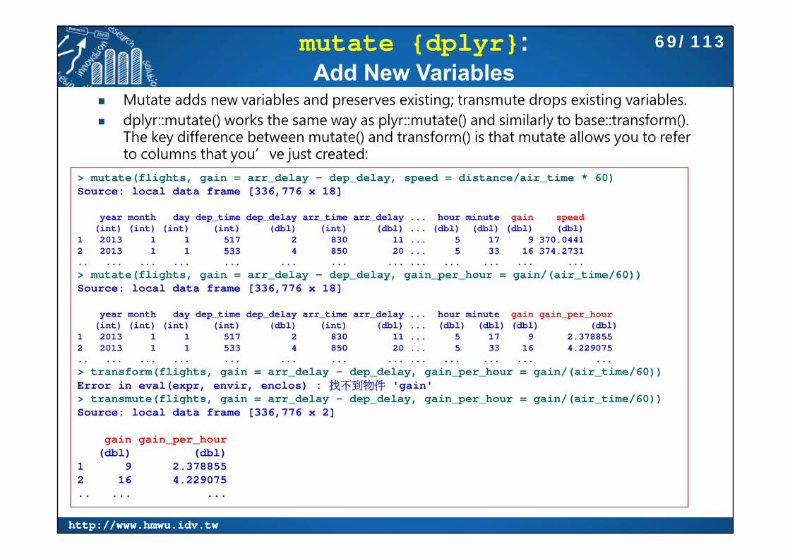
mutate {dplyr}: Add New Variables
Mutate adds new variables and preserves existing; transmute drops existing variables. dplyr::mutate() works the same way as plyr::mutate() and similarly to base::transform().
The key difference between mutate() and transform() is that mutate allows you to refer to columns that you’ve just created:
> mutate(flights, gain = arr_delay - dep_delay, speed = distance/air_time * 60)Source: local data frame [336,776 x 18]
year month day dep_time dep_delay arr_time arr_delay ... hour minute gain speed(int) (int) (int) (int) (dbl) (int) (dbl) ... (dbl) (dbl) (dbl) (dbl)
1 2013 1 1 517 2 830 11 ... 5 17 9 370.04412 2013 1 1 533 4 850 20 ... 5 33 16 374.2731.. ... ... ... ... ... ... ... ... ... ... ... ...> mutate(flights, gain = arr_delay - dep_delay, gain_per_hour = gain/(air_time/60))Source: local data frame [336,776 x 18]
year month day dep_time dep_delay arr_time arr_delay ... hour minute gain gain_per_hour(int) (int) (int) (int) (dbl) (int) (dbl) ... (dbl) (dbl) (dbl) (dbl)
1 2013 1 1 517 2 830 11 ... 5 17 9 2.3788552 2013 1 1 533 4 850 20 ... 5 33 16 4.229075.. ... ... ... ... ... ... ... ... ... ... ... ...> transform(flights, gain = arr_delay - dep_delay, gain_per_hour = gain/(air_time/60))Error in eval(expr, envir, enclos) : 找不到物件 'gain'> transmute(flights, gain = arr_delay - dep_delay, gain_per_hour = gain/(air_time/60))Source: local data frame [336,776 x 2]
gain gain_per_hour(dbl) (dbl)
1 9 2.3788552 16 4.229075.. ... ...
69/113

http://www.hmwu.idv.twhttp://www.hmwu.idv.tw
summarise{dplyr}: Summarise Multiple Values to A Single Value
summarise() collapses a data frame to a single row (this is exactly equivalent to plyr::summarise()).
> head(mtcars, 3)mpg cyl disp hp drat wt qsec vs am gear carb
Mazda RX4 21.0 6 160 110 3.90 2.620 16.46 0 1 4 4Mazda RX4 Wag 21.0 6 160 110 3.90 2.875 17.02 0 1 4 4Datsun 710 22.8 4 108 93 3.85 2.320 18.61 1 1 4 1> group_by(mtcars, cyl)Source: local data frame [32 x 11]Groups: cyl [3]
mpg cyl disp hp drat wt qsec vs am gear carb(dbl) (dbl) (dbl) (dbl) (dbl) (dbl) (dbl) (dbl) (dbl) (dbl) (dbl)
1 21.0 6 160.0 110 3.90 2.620 16.46 0 1 4 42 21.0 6 160.0 110 3.90 2.875 17.02 0 1 4 4.. ... ... ... ... ... ... ... ... ... ... ...> summarise(group_by(mtcars, cyl), m = mean(disp), sd = sd(disp))Source: local data frame [3 x 3]
cyl m sd(dbl) (dbl) (dbl)
1 4 105.1364 26.871592 6 183.3143 41.562463 8 353.1000 67.77132
> summarise(flights, delay = mean(dep_delay, na.rm = TRUE))Source: local data frame [1 x 1]
delay(dbl)
1 12.63907
> mean(flights$dep_delay, na.rm=T)[1] 12.63907
70/113

http://www.hmwu.idv.twhttp://www.hmwu.idv.tw
sample_n{dplyr}, sample_frac{dplyr}:Randomly Sample Rows
> sample_n(iris, 5)Source: local data frame [5 x 5]
Sepal.Length Sepal.Width Petal.Length Petal.Width Species(dbl) (dbl) (dbl) (dbl) (fctr)
1 6.7 3.0 5.2 2.3 virginica2 6.3 2.5 4.9 1.5 versicolor3 6.9 3.1 5.1 2.3 virginica4 6.2 3.4 5.4 2.3 virginica5 5.0 3.5 1.6 0.6 setosa> sample_frac(iris, 0.05)Source: local data frame [8 x 5]
Sepal.Length Sepal.Width Petal.Length Petal.Width Species(dbl) (dbl) (dbl) (dbl) (fctr)
1 5.0 3.4 1.6 0.4 setosa2 7.0 3.2 4.7 1.4 versicolor3 5.6 3.0 4.5 1.5 versicolor4 7.7 2.6 6.9 2.3 virginica5 5.1 3.7 1.5 0.4 setosa6 5.0 3.3 1.4 0.2 setosa7 5.1 3.5 1.4 0.3 setosa8 6.4 2.9 4.3 1.3 versicolor
71/113

http://www.hmwu.idv.twhttp://www.hmwu.idv.tw
group_by{dplyr}:Grouped Operations
> by_tailnum <- group_by(flights, tailnum)> by_tailnumSource: local data frame [336,776 x 16]Groups: tailnum [4044]
year month day dep_time dep_delay arr_time arr_delay carrier tailnum flight origin dest air_time distance(int) (int) (int) (int) (dbl) (int) (dbl) (chr) (chr) (int) (chr) (chr) (dbl) (dbl)
1 2013 1 1 517 2 830 11 UA N14228 1545 EWR IAH 227 14002 2013 1 1 533 4 850 20 UA N24211 1714 LGA IAH 227 1416.. ... ... ... ... ... ... ... ... ... ... ... ... ... ...Variables not shown: hour (dbl), minute (dbl)
> delay <- summarise(by_tailnum,+ count = n(),+ dist = mean(distance, na.rm = TRUE),+ delay = mean(arr_delay, na.rm = TRUE))> delaySource: local data frame [4,044 x 4]
tailnum count dist delay(chr) (int) (dbl) (dbl)
1 2512 710.2576 NaN2 D942DN 4 854.5000 31.50000003 N0EGMQ 371 676.1887 9.9829545.. ... ... ... ...> delay <- filter(delay, count > 20, dist < 2000)> delaySource: local data frame [2,962 x 4]
tailnum count dist delay(chr) (int) (dbl) (dbl)
1 2512 710.2576 NaN2 N0EGMQ 371 676.1887 9.98295453 N10156 153 757.9477 12.7172414.. ... ... ... ...
Group the complete dataset by planes numbers (tailnum) and then summarise each plane by counting the number of flights (count = n()) and computing the average distance (dist = mean(Distance, na.rm = TRUE)) and arrival delay (delay = mean(ArrDelay, na.rm = TRUE)).
72/113

http://www.hmwu.idv.twhttp://www.hmwu.idv.tw
Visualize the Resultsggplot(delay, aes(dist, delay)) +
geom_point(aes(size = count), alpha = 1/2) +geom_smooth() +scale_size_area()
The average delay is only slightly related to the average distance flown by a plane.
73/113
http://www.hmwu.idv.twhttp://www.hmwu.idv.tw
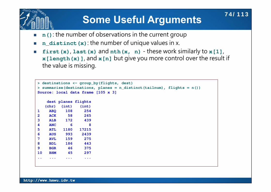
Some Useful Arguments n(): the number of observations in the current group n_distinct(x): the number of unique values in x. first(x), last(x) and nth(x, n) - these work similarly to x[1],
x[length(x)], and x[n] but give you more control over the result if the value is missing.
> destinations <- group_by(flights, dest)> summarise(destinations, planes = n_distinct(tailnum), flights = n())Source: local data frame [105 x 3]
dest planes flights(chr) (int) (int)
1 ABQ 108 2542 ACK 58 2653 ALB 172 4394 ANC 6 85 ATL 1180 172156 AUS 993 24397 AVL 159 2758 BDL 186 4439 BGR 46 37510 BHM 45 297.. ... ... ...
74/113

http://www.hmwu.idv.twhttp://www.hmwu.idv.tw
Summarise{dplyr}with Some Other Helpful Functions
> daily <- group_by(flights, year, month, day)> (per_day <- summarise(daily, flights = n()))Source: local data frame [365 x 4]Groups: year, month [?]
year month day flights(int) (int) (int) (int)
1 2013 1 1 8422 2013 1 2 9433 2013 1 3 9144 2013 1 4 9155 2013 1 5 7206 2013 1 6 8327 2013 1 7 9338 2013 1 8 8999 2013 1 9 90210 2013 1 10 932.. ... ... ... ...
> (per_year <- summarise(per_month, flights = sum(flights)))Source: local data frame [1 x 2]
year flights(int) (int)
1 2013 336776
> (per_month <- summarise(per_day, flights = sum(flights)))Source: local data frame [12 x 3]Groups: year [?]
year month flights(int) (int) (int)
1 2013 1 270042 2013 2 249513 2013 3 288344 2013 4 283305 2013 5 287966 2013 6 282437 2013 7 294258 2013 8 293279 2013 9 2757410 2013 10 2888911 2013 11 2726812 2013 12 28135
75/113

http://www.hmwu.idv.twhttp://www.hmwu.idv.tw
Chaining (Pipe operator: %>%)
https://cran.rstudio.com/web/packages/dplyr/vignettes/introduction.html
a1 <- group_by(flights, year, month, day)a2 <- select(a1, arr_delay, dep_delay)a3 <- summarise(a2,
arr = mean(arr_delay, na.rm = TRUE),dep = mean(dep_delay, na.rm = TRUE))
a4 <- filter(a3, arr > 30 | dep > 30)
filter(summarise(
select(group_by(flights, year, month, day),arr_delay, dep_delay
),arr = mean(arr_delay, na.rm = TRUE),dep = mean(dep_delay, na.rm = TRUE)
),arr > 30 | dep > 30
)
flights %>%group_by(year, month, day) %>%select(arr_delay, dep_delay) %>%summarise(
arr = mean(arr_delay, na.rm = TRUE),dep = mean(dep_delay, na.rm = TRUE)
) %>%filter(arr > 30 | dep > 30)
dplyr provides the %>% operator. x %>% f(y) turns into f(x, y) so you can use it to rewrite multiple operations that you can read left-to-right, top-to-bottom.
This is difficult to read because the order of the operations is from inside to out. Thus, the arguments are a long way away from the function.
76/113

http://www.hmwu.idv.twhttp://www.hmwu.idv.tw
Join in dplyr join{dplyr}: anti_join, full_join, inner_join,
left_join, right_join, semi_join.
semi_join(): return all rows from x where there are matching values in y, keeping just columns from x. A semi join differs from an inner join because an inner join
will return one row of x for each matching row of y, where a semi join will never duplicate rows of x.
anti_join(): return all rows from x where there are not matching values in y, keeping just columns from x.
The difference between merge and join{dplyr} : dplyr的join不會去比對by variable都是NA的情況。
77/113

http://www.hmwu.idv.twhttp://www.hmwu.idv.tw
R Package tidyr: Easily Tidy Data
Some references https://github.com/hadley/tidyr/tree/master/vignettes https://cran.r-project.org/web/packages/tidyr/vignettes/tidy-data.html blog.rstudio.org/2014/07/22/introducing-tidyr/ http://garrettgman.github.io/tidying/ https://rpubs.com/bradleyboehmke/data_wrangling
Hadley Wickham, Tidy Data, Journal of Statistical Software. August 2014, Volume 59, Issue 10.
78/113

http://www.hmwu.idv.twhttp://www.hmwu.idv.tw
Data Semantics (語義學) In addition to appearance, we need a way to describe the
underlying semantics, or meaning, of the values displayed in the table.
Data tidying is to structure datasets to facilitate analysis.
Tidy datasets provide a standardized way to link the structure of a dataset (its physical layout) with its semantics (its meaning).
A dataset is a collection of values, usually either numbers (if quantitative) or strings (if qualitative). Values are organised in two ways. Every value belongs to a variable and an observation. A variable contains all values that measure the same underlying
attribute (like height, temperature, duration) across units. An observation contains all values measured on the same unit (like a
person, or a day, or a race) across attributes.
https://cran.r-project.org/web/packages/tidyr/vignettes/tidy-data.html
79/113
http://www.hmwu.idv.twhttp://www.hmwu.idv.tw
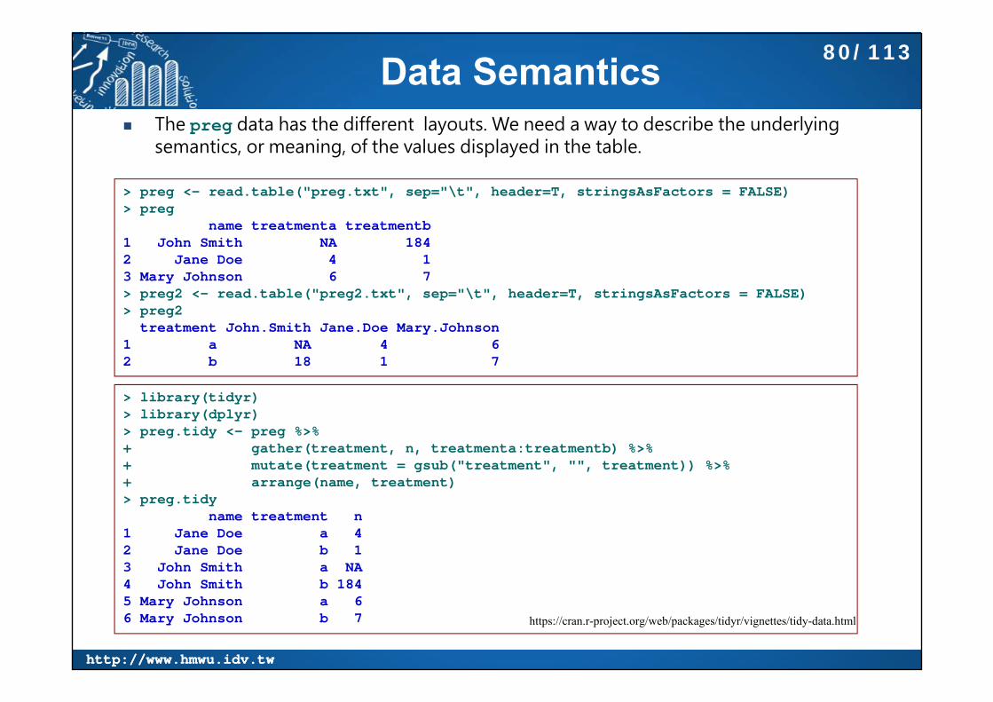
Data Semantics The preg data has the different layouts. We need a way to describe the underlying
semantics, or meaning, of the values displayed in the table.
> preg <- read.table("preg.txt", sep="\t", header=T, stringsAsFactors = FALSE)> preg
name treatmenta treatmentb1 John Smith NA 1842 Jane Doe 4 13 Mary Johnson 6 7> preg2 <- read.table("preg2.txt", sep="\t", header=T, stringsAsFactors = FALSE)> preg2
treatment John.Smith Jane.Doe Mary.Johnson1 a NA 4 62 b 18 1 7
> library(tidyr)> library(dplyr)> preg.tidy <- preg %>% + gather(treatment, n, treatmenta:treatmentb) %>%+ mutate(treatment = gsub("treatment", "", treatment)) %>%+ arrange(name, treatment)> preg.tidy
name treatment n1 Jane Doe a 42 Jane Doe b 13 John Smith a NA4 John Smith b 1845 Mary Johnson a 66 Mary Johnson b 7 https://cran.r-project.org/web/packages/tidyr/vignettes/tidy-data.html
80/113
http://www.hmwu.idv.twhttp://www.hmwu.idv.tw
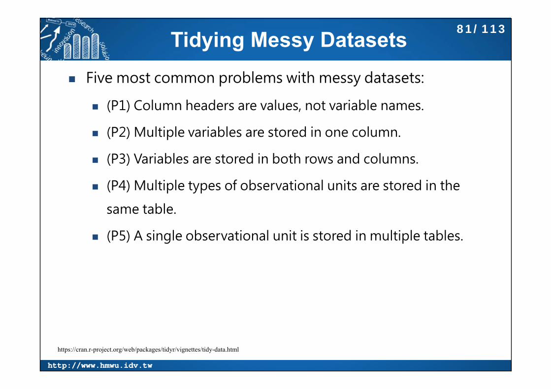
Tidying Messy Datasets Five most common problems with messy datasets:
(P1) Column headers are values, not variable names.
(P2) Multiple variables are stored in one column.
(P3) Variables are stored in both rows and columns.
(P4) Multiple types of observational units are stored in the
same table.
(P5) A single observational unit is stored in multiple tables.
https://cran.r-project.org/web/packages/tidyr/vignettes/tidy-data.html
81/113

http://www.hmwu.idv.twhttp://www.hmwu.idv.tw
gather {tidyr}: Gather Columns into Key-Value Pairs
gather(data, key, value, ..., na.rm = FALSE, convert = FALSE)
data:A data frame.key,value: Names of key and value columns to create in output....: Specification of columns to gather. Use bare variable names. Select all variables between x and z with x:z, exclude y with -y.
> xdata <- data.frame(Group=letters[1:4], matrix(rnorm(12), ncol=3))> xdata
Group X1 X2 X31 a 2.9077373 -0.6077071 -0.50202092 b 1.1250308 1.9919512 -0.54291163 c 1.0895884 1.1823842 0.68111484 d -0.3249144 1.5894412 -1.4850463> gather(xdata, key = KEY, value = VALUE, -Group)
Group KEY VALUE1 a X1 2.90773732 b X1 1.12503083 c X1 1.08958844 d X1 -0.32491445 a X2 -0.60770716 b X2 1.99195127 c X2 1.18238428 d X2 1.58944129 a X3 -0.502020910 b X3 -0.542911611 c X3 0.681114812 d X3 -1.4850463
82/113

http://www.hmwu.idv.twhttp://www.hmwu.idv.tw
gather {tidyr}, Example (1)
> gather(xdata, key = KEY, value = VALUE)KEY VALUE
1 Group a2 Group b3 Group c4 Group d5 X1 2.907737254942516 X1 1.125030762220757 X1 1.089588428515678 X1 -0.3249144177788459 X2 -0.60770710038195810 X2 1.9919511996552411 X2 1.1823842333904312 X2 1.5894411573867513 X3 -0.50202093472687814 X3 -0.54291163576156315 X3 0.6811148329725516 X3 -1.48504628535113Warning message:attributes are not identical across measure variables; they will be dropped > gather(xdata, key = KEY, value = VALUE, Group)
X1 X2 X3 KEY VALUE1 2.9077373 -0.6077071 -0.5020209 Group a2 1.1250308 1.9919512 -0.5429116 Group b3 1.0895884 1.1823842 0.6811148 Group c4 -0.3249144 1.5894412 -1.4850463 Group d> gather(xdata, key = KEY, value = VALUE, X1)Group X2 X3 KEY VALUE
1 a -0.6077071 -0.5020209 X1 2.90773732 b 1.9919512 -0.5429116 X1 1.12503083 c 1.1823842 0.6811148 X1 1.08958844 d 1.5894412 -1.4850463 X1 -0.3249144
> gather(xdata, key = KEY, value = VALUE, X1, X2)Group X3 KEY VALUE
1 a -0.5020209 X1 2.90773732 b -0.5429116 X1 1.12503083 c 0.6811148 X1 1.08958844 d -1.4850463 X1 -0.32491445 a -0.5020209 X2 -0.60770716 b -0.5429116 X2 1.99195127 c 0.6811148 X2 1.18238428 d -1.4850463 X2 1.5894412> gather(xdata, key = KEY, value = VALUE, X1:X3)
Group KEY VALUE1 a X1 2.90773732 b X1 1.12503083 c X1 1.08958844 d X1 -0.32491445 a X2 -0.60770716 b X2 1.99195127 c X2 1.18238428 d X2 1.58944129 a X3 -0.502020910 b X3 -0.542911611 c X3 0.681114812 d X3 -1.4850463
83/113
http://www.hmwu.idv.twhttp://www.hmwu.idv.tw
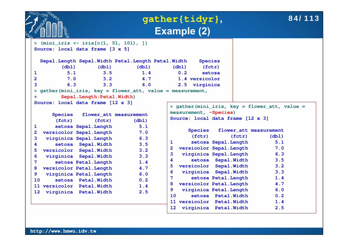
gather{tidyr}, Example (2)
> (mini_iris <- iris[c(1, 51, 101), ])Source: local data frame [3 x 5]
Sepal.Length Sepal.Width Petal.Length Petal.Width Species(dbl) (dbl) (dbl) (dbl) (fctr)
1 5.1 3.5 1.4 0.2 setosa2 7.0 3.2 4.7 1.4 versicolor3 6.3 3.3 6.0 2.5 virginica> gather(mini_iris, key = flower_att, value = measurement,+ Sepal.Length:Petal.Width)Source: local data frame [12 x 3]
Species flower_att measurement(fctr) (fctr) (dbl)
1 setosa Sepal.Length 5.12 versicolor Sepal.Length 7.03 virginica Sepal.Length 6.34 setosa Sepal.Width 3.55 versicolor Sepal.Width 3.26 virginica Sepal.Width 3.37 setosa Petal.Length 1.48 versicolor Petal.Length 4.79 virginica Petal.Length 6.010 setosa Petal.Width 0.211 versicolor Petal.Width 1.412 virginica Petal.Width 2.5
> gather(mini_iris, key = flower_att, value = measurement, -Species)Source: local data frame [12 x 3]
Species flower_att measurement(fctr) (fctr) (dbl)
1 setosa Sepal.Length 5.12 versicolor Sepal.Length 7.03 virginica Sepal.Length 6.34 setosa Sepal.Width 3.55 versicolor Sepal.Width 3.26 virginica Sepal.Width 3.37 setosa Petal.Length 1.48 versicolor Petal.Length 4.79 virginica Petal.Length 6.010 setosa Petal.Width 0.211 versicolor Petal.Width 1.412 virginica Petal.Width 2.5
84/113

http://www.hmwu.idv.twhttp://www.hmwu.idv.tw
(P1) Column Headers are Values pew.csv dataset explores the relationship between income and religion in the US. It
comes from a report[1] produced by the Pew Research Center, an American think-tank that collects data on attitudes to topics ranging from religion to the internet, and produces many reports that contain datasets in this format.
> pew <- tbl_df(read.csv("pew.csv", stringsAsFactors = FALSE, check.names = FALSE))> pewSource: local data frame [18 x 11]
religion <$10k $10-20k $20-30k $30-40k $40-50k $50-75k $75-100k $100-150k(chr) (int) (int) (int) (int) (int) (int) (int) (int)
1 Agnostic 27 34 60 81 76 137 122 1092 Atheist 12 27 37 52 35 70 73 593 Buddhist 27 21 30 34 33 58 62 394 Catholic 418 617 732 670 638 1116 949 7925 Don\xe2\u0080 know/refused 15 14 15 11 10 35 21 176 Evangelical Prot 575 869 1064 982 881 1486 949 7237 Hindu 1 9 7 9 11 34 47 488 Historically Black Prot 228 244 236 238 197 223 131 819 Jehovah's Witness 20 27 24 24 21 30 15 1110 Jewish 19 19 25 25 30 95 69 8711 Mainline Prot 289 495 619 655 651 1107 939 75312 Mormon 29 40 48 51 56 112 85 4913 Muslim 6 7 9 10 9 23 16 814 Orthodox 13 17 23 32 32 47 38 4215 Other Christian 9 7 11 13 13 14 18 1416 Other Faiths 20 33 40 46 49 63 46 4017 Other World Religions 5 2 3 4 2 7 3 418 Unaffiliated 217 299 374 365 341 528 407 321Variables not shown: >150k (int), Don't know/refused (int)
[1] http://www.pewforum.org/religious-landscape-study/This dataset has three variables, religion, income and frequency. To tidy it, we need to gather the non-variable columns into a two-column key-value pair. https://cran.r-project.org/web/packages/tidyr/vignettes/tidy-data.html
pew %>%gather(income, frequency, -religion)
#> Source: local data frame [180 x 3]#> #> religion income frequency#> (chr) (chr) (int)#> 1 Agnostic <$10k 27#> 2 Atheist <$10k 12
85/113

http://www.hmwu.idv.twhttp://www.hmwu.idv.tw
gather{tidyr}, Example (3)
> stockstime X Y Z
1 2009-01-01 -1.33362673 3.6589529 0.15090512 2009-01-02 0.21038002 -0.1723368 6.82479033 2009-01-03 -0.16678875 -1.9590724 2.56991894 2009-01-04 -0.15690945 -2.1929030 -1.80191895 2009-01-05 0.27238365 0.7867679 -2.63809886 2009-01-06 1.78031897 2.5329838 8.81527597 2009-01-07 -2.06912971 2.6226384 3.91679528 2009-01-08 -1.02148600 -2.5632745 2.84963959 2009-01-09 0.32494284 -3.4165507 -6.101689910 2009-01-10 -0.04459401 1.0952851 -3.2018426> # stocks %>% gather(stock, price, -time)> stocks.ga <- gather(stocks, key = stock,
value = price, -time)> stocks.ga
time stock price1 2009-01-01 X -1.333626732 2009-01-02 X 0.21038002...10 2009-01-10 X -0.0445940111 2009-01-01 Y 3.6589529112 2009-01-02 Y -0.17233676...19 2009-01-09 Y -3.4165506520 2009-01-10 Y 1.09528513...29 2009-01-09 Z -6.1016898630 2009-01-10 Z -3.20184256
stocks <- data.frame(time = as.Date('2009-01-01') + 0:9,X = rnorm(10, 0, 1),Y = rnorm(10, 0, 2),Z = rnorm(10, 0, 4)
)
This form is tidy because each column represents a variable and each row represents an observation, in this case a demographic unit corresponding to a combination of religion and income.
https://cran.r-project.org/web/packages/tidyr/vignettes/tidy-data.html
86/113

http://www.hmwu.idv.twhttp://www.hmwu.idv.tw
Billboard Dataset Billboard dataset records the date a song first entered the billboard top
100. It has variables for artist, track, date.entered, rank and week. The rank in each week after it enters the top 100 is recorded in 75 columns, wk1 to wk75.
This form of storage is useful for data entry. It reduces duplication since otherwise each song in each week would need its own row, and song metadata like title and artist would need to be repeated.
> billboard <- tbl_df(read.csv("billboard.csv", stringsAsFactors = FALSE))> billboardSource: local data frame [317 x 81]
year artist track time date.entered wk1 wk2(int) (chr) (chr) (chr) (chr) (int) (int)
1 2000 2 Pac Baby Don't Cry (Keep... 4:22 2000-02-26 87 822 2000 2Ge+her The Hardest Part Of ... 3:15 2000-09-02 91 87...10 2000 Adams, Yolanda Open My Heart 5:30 2000-08-26 76 76.. ... ... ... ... ... ... ...Variables not shown: wk3 (int), wk4 (int), wk5 (int), wk6 (int), wk7 (int), wk8...
(lgl), wk74 (lgl), wk75 (lgl), wk76 (lgl)
https://cran.r-project.org/web/packages/tidyr/vignettes/tidy-data.html
87/113

http://www.hmwu.idv.twhttp://www.hmwu.idv.tw
Tidy Billboard Dataset by gather()
Tidy Billboard dataset by gathering together all the wk columns. The column names give the week and the values are the ranks.
Use na.rm to drop any missing values (weeks that the song wasnot in the charts) from the gather columns.
> billboard2 <- billboard %>% + gather(week, rank, wk1:wk76, na.rm = TRUE)> billboard2Source: local data frame [5,307 x 7]
year artist track time date.entered week rank(int) (chr) (chr) (chr) (chr) (fctr) (int)
1 2000 2 Pac Baby Don't Cry (Keep... 4:22 2000-02-26 wk1 872 2000 2Ge+her The Hardest Part Of ... 3:15 2000-09-02 wk1 913 2000 3 Doors Down Kryptonite 3:53 2000-04-08 wk1 814 2000 3 Doors Down Loser 4:24 2000-10-21 wk1 765 2000 504 Boyz Wobble Wobble 3:35 2000-04-15 wk1 576 2000 98^0 Give Me Just One Nig... 3:24 2000-08-19 wk1 517 2000 A*Teens Dancing Queen 3:44 2000-07-08 wk1 978 2000 Aaliyah I Don't Wanna 4:15 2000-01-29 wk1 849 2000 Aaliyah Try Again 4:03 2000-03-18 wk1 5910 2000 Adams, Yolanda Open My Heart 5:30 2000-08-26 wk1 76.. ... ... ... ... ... ... ...
https://cran.r-project.org/web/packages/tidyr/vignettes/tidy-data.html
88/113

http://www.hmwu.idv.twhttp://www.hmwu.idv.tw
Cleaning Billboard Dataset
cleaning: converting the week variable to a number, and figuring out the date corresponding to each week on the charts.> billboard3 <- billboard2 %>%+ mutate(+ week = extract_numeric(week),+ date = as.Date(date.entered) + 7 * (week - 1)) %>%+ select(-date.entered)> billboard3Source: local data frame [5,307 x 7]
year artist track time week rank date(int) (chr) (chr) (chr) (dbl) (int) (date)
1 2000 2 Pac Baby Don't Cry (Keep... 4:22 1 87 2000-02-262 2000 2Ge+her The Hardest Part Of ... 3:15 1 91 2000-09-023 2000 3 Doors Down Kryptonite 3:53 1 81 2000-04-084 2000 3 Doors Down Loser 4:24 1 76 2000-10-215 2000 504 Boyz Wobble Wobble 3:35 1 57 2000-04-156 2000 98^0 Give Me Just One Nig... 3:24 1 51 2000-08-197 2000 A*Teens Dancing Queen 3:44 1 97 2000-07-088 2000 Aaliyah I Don't Wanna 4:15 1 84 2000-01-299 2000 Aaliyah Try Again 4:03 1 59 2000-03-1810 2000 Adams, Yolanda Open My Heart 5:30 1 76 2000-08-26.. ... ... ... ... ... ... ...
https://cran.r-project.org/web/packages/tidyr/vignettes/tidy-data.html
89/113

http://www.hmwu.idv.twhttp://www.hmwu.idv.tw
arrange{dplyr}: Arrange Rows by Variables
Sort the data by artist, track and week.> billboard3 %>% arrange(artist, track, week)Source: local data frame [5,307 x 7]
year artist track time week rank date(int) (chr) (chr) (chr) (dbl) (int) (date)
1 2000 2 Pac Baby Don't Cry (Keep... 4:22 1 87 2000-02-262 2000 2 Pac Baby Don't Cry (Keep... 4:22 2 82 2000-03-043 2000 2 Pac Baby Don't Cry (Keep... 4:22 3 72 2000-03-11...9 2000 2Ge+her The Hardest Part Of ... 3:15 2 87 2000-09-0910 2000 2Ge+her The Hardest Part Of ... 3:15 3 92 2000-09-16.. ... ... ... ... ... ... ...
> billboard3 %>% arrange(date, rank)Source: local data frame [5,307 x 7]
year artist track time week rank date(int) (chr) (chr) (chr) (dbl) (int) (date)
1 2000 Lonestar Amazed 4:25 1 81 1999-06-052 2000 Lonestar Amazed 4:25 2 54 1999-06-123 2000 Lonestar Amazed 4:25 3 44 1999-06-19...9 2000 Lonestar Amazed 4:25 8 29 1999-07-2410 2000 Amber Sexual 4:38 2 99 1999-07-24.. ... ... ... ... ... ... ...
Or by date and rank.
90/113
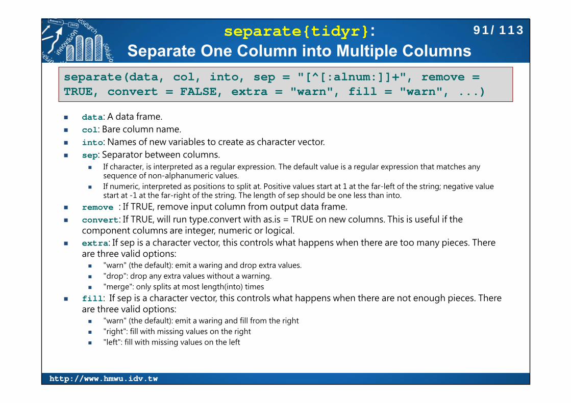
http://www.hmwu.idv.twhttp://www.hmwu.idv.tw
separate{tidyr}: Separate One Column into Multiple Columns
data: A data frame. col: Bare column name. into: Names of new variables to create as character vector. sep: Separator between columns.
If character, is interpreted as a regular expression. The default value is a regular expression that matches any sequence of non-alphanumeric values.
If numeric, interpreted as positions to split at. Positive values start at 1 at the far-left of the string; negative value start at -1 at the far-right of the string. The length of sep should be one less than into.
remove : If TRUE, remove input column from output data frame. convert: If TRUE, will run type.convert with as.is = TRUE on new columns. This is useful if the
component columns are integer, numeric or logical. extra: If sep is a character vector, this controls what happens when there are too many pieces. There
are three valid options: "warn" (the default): emit a waring and drop extra values. "drop": drop any extra values without a warning. "merge": only splits at most length(into) times
fill: If sep is a character vector, this controls what happens when there are not enough pieces. There are three valid options: "warn" (the default): emit a waring and fill from the right "right": fill with missing values on the right "left": fill with missing values on the left
separate(data, col, into, sep = "[^[:alnum:]]+", remove = TRUE, convert = FALSE, extra = "warn", fill = "warn", ...)
91/113

http://www.hmwu.idv.twhttp://www.hmwu.idv.tw
separate {dplyr}
> (df <- data.frame(x = c(NA, "a.b", "a.d", "b.c")))x
1 <NA>2 a.b3 a.d4 b.c> df %>% separate(x, c("X1", "X2"))
X1 X21 <NA> <NA>2 a b3 a d4 b c> # separate(df, x, c("X1", "X2"))>> (df <- data.frame(x = c("a", "a b", "a b c", NA)))
x1 a2 a b3 a b c4 <NA>> df %>% separate(x, c("X1", "X2"))
X1 X21 a <NA>2 a b3 a b4 <NA> <NA>Warning messages:1: Too many values at 1 locations: 3 2: Too few values at 1 locations: 1
> (df %>% separate(x, c("X1", "X2"), extra = "drop", fill = "right"))
X1 X21 a <NA>2 a b3 a b4 <NA> <NA>>
no warnings
separate() makes it easy to split a compound variables into individual variables. You can either pass it a regular expression to split on (the default is to split on non-alphanumeric columns), or a vector of character positions.
92/113

http://www.hmwu.idv.twhttp://www.hmwu.idv.tw
separate{dplyr}
> dfx
1 a2 a b3 a b c4 <NA>> df %>% separate(x, c("X1", "X2"), extra = "merge", fill = "left")
X1 X21 <NA> a2 a b3 a b c4 <NA> <NA>> > (df <- data.frame(x = c("x: 123", "y: error: 7")))
x1 x: 1232 y: error: 7> df %>% separate(x, c("Key", "Value"), ": ", extra = "merge")
Key Value1 x 1232 y error: 7
use extra = "merge" to split specified number of times
93/113

http://www.hmwu.idv.twhttp://www.hmwu.idv.tw
(P2) Multiple Variables Stored in One Column
Tuberculosis dataset comes from the World Health Organisation, and records the counts of confirmed tuberculosis cases by country, year, and demographic group. The demographic groups are broken down by sex (m, f) and age (0-14, 15-25, 25-34, 35-44, 45-54, 55-64, unknown).
> tb <- tbl_df(read.csv("tb.csv", stringsAsFactors = FALSE))> tbSource: local data frame [5,769 x 22]
iso2 year m04 m514 m014 m1524 m2534 m3544 m4554 m5564 m65 mu f04(chr) (int) (int) (int) (int) (int) (int) (int) (int) (int) (int) (int) (int)
1 AD 1989 NA NA NA NA NA NA NA NA NA NA NA2 AD 1990 NA NA NA NA NA NA NA NA NA NA NA3 AD 1991 NA NA NA NA NA NA NA NA NA NA NA4 AD 1992 NA NA NA NA NA NA NA NA NA NA NA5 AD 1993 NA NA NA NA NA NA NA NA NA NA NA6 AD 1994 NA NA NA NA NA NA NA NA NA NA NA7 AD 1996 NA NA 0 0 0 4 1 0 0 NA NA8 AD 1997 NA NA 0 0 1 2 2 1 6 NA NA9 AD 1998 NA NA 0 0 0 1 0 0 0 NA NA10 AD 1999 NA NA 0 0 0 1 1 0 0 NA NA.. ... ... ... ... ... ... ... ... ... ... ... ... ...Variables not shown: f514 (int), f014 (int), f1524 (int), f2534 (int), f3544
(int), f4554 (int), f5564 (int), f65 (int), fu (int)
https://cran.r-project.org/web/packages/tidyr/vignettes/tidy-data.html
94/113

http://www.hmwu.idv.twhttp://www.hmwu.idv.tw
Tidy Tuberculosis Dataset
> tb2 <- tb %>% gather(demo, n, -iso2, -year, na.rm = TRUE)> tb2Source: local data frame [35,750 x 4]
iso2 year demo n(chr) (int) (fctr) (int)
1 AD 2005 m04 02 AD 2006 m04 03 AD 2008 m04 04 AE 2006 m04 05 AE 2007 m04 06 AE 2008 m04 07 AG 2007 m04 08 AL 2005 m04 09 AL 2006 m04 110 AL 2007 m04 0.. ... ... ... ...
gather up the non-variable columns
> tb3 <- tb2 %>% separate(demo, c("sex", "age"), 1)> tb3Source: local data frame [35,750 x 5]
iso2 year sex age n(chr) (int) (chr) (chr) (int)
1 AD 2005 m 04 02 AD 2006 m 04 03 AD 2008 m 04 04 AE 2006 m 04 05 AE 2007 m 04 06 AE 2008 m 04 07 AG 2007 m 04 08 AL 2005 m 04 09 AL 2006 m 04 110 AL 2007 m 04 0.. ... ... ... ... ...
Column headers in this format are often separated by a non-alphanumeric character (e.g. ., -, _, :), or have a fixed width format, like in this dataset. In this case we want to split after the first character:
Storing the values in this form resolves a problem in the original data. We want to compare rates, not counts, which means we need to know the population. In the original format, there is no easy way to add a population variable. It has to be stored in a separate table, which makes it hard to correctly match populations to counts. In tidy form, adding variables for population and rate is easy because they're just additional columns.
https://cran.r-project.org/web/packages/tidyr/vignettes/tidy-data.html
95/113
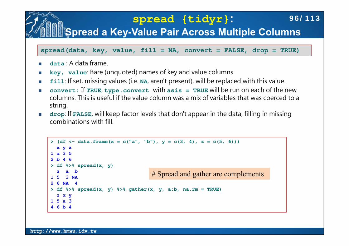
http://www.hmwu.idv.twhttp://www.hmwu.idv.tw
spread {tidyr}: Spread a Key-Value Pair Across Multiple Columns
data : A data frame. key, value: Bare (unquoted) names of key and value columns. fill: If set, missing values (i.e. NA, aren't present), will be replaced with this value. convert: If TRUE, type.convert with asis = TRUE will be run on each of the new
columns. This is useful if the value column was a mix of variables that was coerced to a string.
drop: If FALSE, will keep factor levels that don't appear in the data, filling in missing combinations with fill.
spread(data, key, value, fill = NA, convert = FALSE, drop = TRUE)
> (df <- data.frame(x = c("a", "b"), y = c(3, 4), z = c(5, 6)))x y z
1 a 3 52 b 4 6> df %>% spread(x, y)
z a b1 5 3 NA2 6 NA 4> df %>% spread(x, y) %>% gather(x, y, a:b, na.rm = TRUE)
z x y1 5 a 34 6 b 4
# Spread and gather are complements
96/113

http://www.hmwu.idv.twhttp://www.hmwu.idv.tw
spread {tidyr}, Example
> stockstime X Y Z
1 2009-01-01 -0.63120696 0.7047430 -4.92279972 2009-01-02 0.86850592 3.9330433 2.34104683 2009-01-03 -0.13134067 0.6719418 -3.4463902...10 2009-01-10 -0.86706770 -3.4354217 2.0495285> stocks.ga <- stocks %>% gather(company, price, -time)> stocks.ga
time company price1 2009-01-01 X 0.28362692 2009-01-02 X 0.4151764...29 2009-01-09 Z 4.531983230 2009-01-10 Z 3.0196810> stocks.ga %>% spread(company, price)
time X Y Z1 2009-01-01 -0.63120696 0.7047430 -4.92279972 2009-01-02 0.86850592 3.9330433 2.3410468...10 2009-01-10 -0.86706770 -3.4354217 2.0495285> stocks.ga %>% spread(time, price)
company 2009-01-01 2009-01-02 2009-01-03 2009-01-04 2009-01-05 2009-01-061 X -0.631207 0.8685059 -0.1313407 0.7155024 0.02419769 -1.8267512 Y 0.704743 3.9330433 0.6719418 -0.4681197 -2.68079953 -1.0769813 Z -4.922800 2.3410468 -3.4463902 -2.9161013 0.75513726 -5.250819
2009-01-07 2009-01-08 2009-01-09 2009-01-101 -0.7436164 0.3965774 2.0627961 -0.86706772 0.2790172 5.7711958 -0.3719509 -3.43542173 -2.4922130 3.6001196 6.6939517 2.0495285
stocks <- data.frame(time = as.Date('2009-01-01') + 0:9,X = rnorm(10, 0, 1),Y = rnorm(10, 0, 2),Z = rnorm(10, 0, 4)
)
97/113

http://www.hmwu.idv.twhttp://www.hmwu.idv.tw
(P3) Variables are Stored in Both Rows and Columns
The daily weather data was from the Global Historical Climatology Network for one weather station (MX17004) in Mexico for five months in 2010.
It has variables in individual columns (id, year, month), spread across columns (day, d1-d31) and across rows (tmin, tmax) (minimum and maximum temperature). Months with fewer than 31 days have structural missing values for the last day(s) of the month.
> weather <- tbl_df(read.csv("weather.csv", stringsAsFactors = FALSE))> weatherSource: local data frame [22 x 35]
id year month element d1 d2 d3 d4 d5 d6 d7 d8(chr) (int) (int) (chr) (dbl) (dbl) (dbl) (dbl) (dbl) (dbl) (dbl) (dbl)
1 MX17004 2010 1 tmax NA NA NA NA NA NA NA NA2 MX17004 2010 1 tmin NA NA NA NA NA NA NA NA3 MX17004 2010 2 tmax NA 27.3 24.1 NA NA NA NA NA...10 MX17004 2010 5 tmin NA NA NA NA NA NA NA NA.. ... ... ... ... ... ... ... ... ... ... ... ...Variables not shown: d9 (lgl), d10 (dbl), d11 (dbl), d12 (lgl), d13 (dbl), d14
(dbl), d15 (dbl), d16 (dbl), d17 (dbl), d18 (lgl), d19 (lgl), d20 (lgl), d21(lgl), d22 (lgl), d23 (dbl), d24 (lgl), d25 (dbl), d26 (dbl), d27 (dbl), d28(dbl), d29 (dbl), d30 (dbl), d31 (dbl)
https://cran.r-project.org/web/packages/tidyr/vignettes/tidy-data.html
98/113

http://www.hmwu.idv.twhttp://www.hmwu.idv.tw
Tidy Weather Dataset> # Tidy the dataset by gathering the day columns> weather2 <- weather %>% gather(day, value, d1:d31, na.rm = TRUE)> weather2Source: local data frame [66 x 6]
id year month element day value(chr) (int) (int) (chr) (fctr) (dbl)
1 MX17004 2010 12 tmax d1 29.92 MX17004 2010 12 tmin d1 13.8...10 MX17004 2010 7 tmin d3 17.5.. ... ... ... ... ... ...
For presentation, missing values weredropped, making them implicit rather than explicit. This is ok because we know how many days are in each month and can easily reconstruct the explicit missing values.
> # do a little cleaning> weather3 <- weather2 %>% + mutate(day = extract_numeric(day)) %>%+ select(id, year, month, day, element, value) %>%+ arrange(id, year, month, day)> weather3Source: local data frame [66 x 6]
id year month day element value(chr) (int) (int) (dbl) (chr) (dbl)
1 MX17004 2010 1 30 tmax 27.82 MX17004 2010 1 30 tmin 14.5...10 MX17004 2010 2 23 tmin 10.7.. ... ... ... ... ... ...
The element column is not a variable; it stores the names of variables. (Not shown in this example are the other meteorological variables prcp (precipitation) and snow (snowfall)).
99/113

http://www.hmwu.idv.twhttp://www.hmwu.idv.tw
Tidy Weather DatasetUse spread() to perform the inverse of gathering by spreading the element and value columns back out into the columns.
> weather3 %>% spread(element, value)Source: local data frame [33 x 6]
id year month day tmax tmin(chr) (int) (int) (dbl) (dbl) (dbl)
1 MX17004 2010 1 30 27.8 14.52 MX17004 2010 2 2 27.3 14.43 MX17004 2010 2 3 24.1 14.44 MX17004 2010 2 11 29.7 13.45 MX17004 2010 2 23 29.9 10.76 MX17004 2010 3 5 32.1 14.27 MX17004 2010 3 10 34.5 16.88 MX17004 2010 3 16 31.1 17.69 MX17004 2010 4 27 36.3 16.710 MX17004 2010 5 27 33.2 18.2.. ... ... ... ... ... ...
This form is tidy: there's one variable in each column, and each row represents one day.
100/113
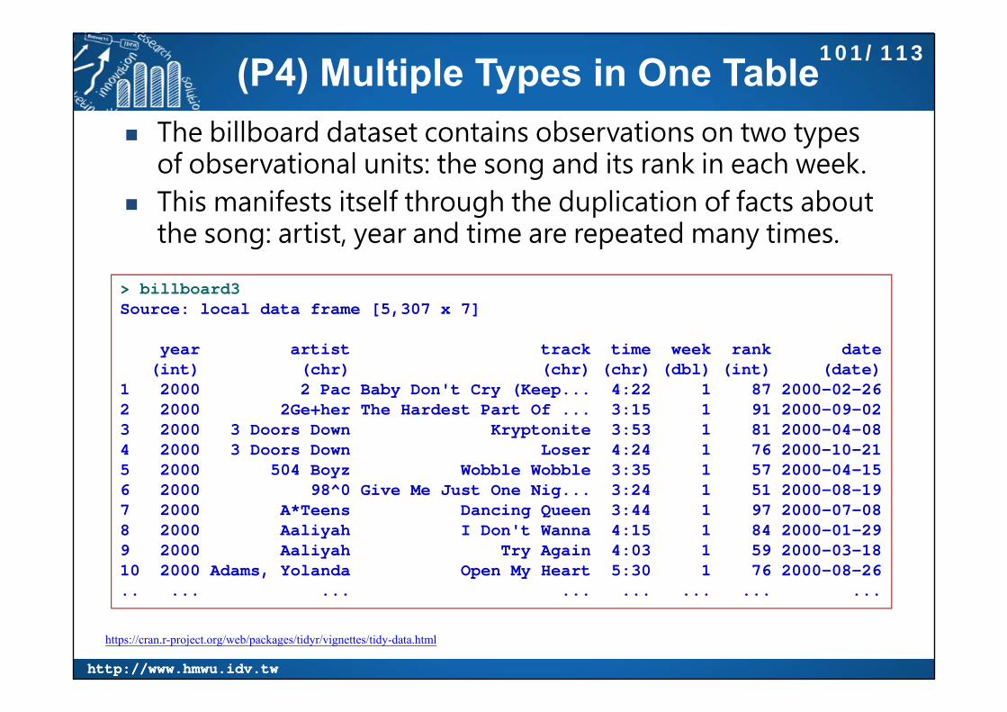
http://www.hmwu.idv.twhttp://www.hmwu.idv.tw
(P4) Multiple Types in One Table The billboard dataset contains observations on two types
of observational units: the song and its rank in each week. This manifests itself through the duplication of facts about
the song: artist, year and time are repeated many times.
> billboard3Source: local data frame [5,307 x 7]
year artist track time week rank date(int) (chr) (chr) (chr) (dbl) (int) (date)
1 2000 2 Pac Baby Don't Cry (Keep... 4:22 1 87 2000-02-262 2000 2Ge+her The Hardest Part Of ... 3:15 1 91 2000-09-023 2000 3 Doors Down Kryptonite 3:53 1 81 2000-04-084 2000 3 Doors Down Loser 4:24 1 76 2000-10-215 2000 504 Boyz Wobble Wobble 3:35 1 57 2000-04-156 2000 98^0 Give Me Just One Nig... 3:24 1 51 2000-08-197 2000 A*Teens Dancing Queen 3:44 1 97 2000-07-088 2000 Aaliyah I Don't Wanna 4:15 1 84 2000-01-299 2000 Aaliyah Try Again 4:03 1 59 2000-03-1810 2000 Adams, Yolanda Open My Heart 5:30 1 76 2000-08-26.. ... ... ... ... ... ... ...
https://cran.r-project.org/web/packages/tidyr/vignettes/tidy-data.html
101/113

http://www.hmwu.idv.twhttp://www.hmwu.idv.tw
Tidy Billboard Dataset This dataset needs to be broken down into two pieces: a song dataset
which stores artist, song name and time, and a ranking dataset which gives the rank of the song in each week.
> #First extract a song dataset> song <- billboard3 %>% + select(artist, track, year, time) %>%+ unique() %>%+ mutate(song_id = row_number())> songSource: local data frame [317 x 5]
artist track year time song_id(chr) (chr) (int) (chr) (int)
1 2 Pac Baby Don't Cry (Keep... 2000 4:22 12 2Ge+her The Hardest Part Of ... 2000 3:15 23 3 Doors Down Kryptonite 2000 3:53 34 3 Doors Down Loser 2000 4:24 45 504 Boyz Wobble Wobble 2000 3:35 56 98^0 Give Me Just One Nig... 2000 3:24 67 A*Teens Dancing Queen 2000 3:44 78 Aaliyah I Don't Wanna 2000 4:15 89 Aaliyah Try Again 2000 4:03 910 Adams, Yolanda Open My Heart 2000 5:30 10.. ... ... ... ... ...
102/113

http://www.hmwu.idv.twhttp://www.hmwu.idv.tw
Tidy Billboard Dataset
> rank <- billboard3 %>%+ left_join(song, c("artist", "track", "year", "time")) %>%+ select(song_id, date, week, rank) %>%+ arrange(song_id, date)> rankSource: local data frame [5,307 x 4]
song_id date week rank(int) (date) (dbl) (int)
1 1 2000-02-26 1 872 1 2000-03-04 2 823 1 2000-03-11 3 724 1 2000-03-18 4 775 1 2000-03-25 5 876 1 2000-04-01 6 947 1 2000-04-08 7 998 2 2000-09-02 1 919 2 2000-09-09 2 8710 2 2000-09-16 3 92.. ... ... ... ...
You could also imagine a week dataset which would record background information about the week, maybe the total number of songs sold or similar "demographic" information.
Normalisation is useful for tidying and eliminating inconsistencies. However, there are few data analysis tools that work directly with relational data, so analysis usually also requires denormalisation or the merging the datasets back into one table.
Then use that to make a rank dataset by replacing repeated song facts with a pointer to song details (a unique song id).
103/113

http://www.hmwu.idv.twhttp://www.hmwu.idv.tw
data.table: Extension of 'data.frame'
Fast aggregation of large data (e.g. 100GB in RAM), fast ordered joins, fast add/modify/delete of columns by group using no copies at all, list columns, a fast friendly file reader and parallel file writer. Offers a natural and flexible syntax, for faster development.
> library(data.table)> # create a data.table object> id <- letters[1:6]> g <- sample(c("F", "M"), 6, replace=T)> s <- sample(0:100, 6, replace=T)> p <- sample(c("T", "F"), 6, replace=T)> DT <- data.table(ID=id, gender=g, score=s, pass=p)> str(DT)Classes ‘data.table’ and 'data.frame': 6 obs. of 4 variables:$ ID : chr "a" "b" "c" "d" ...$ gender: chr "F" "M" "M" "M" ...$ score : int 93 34 3 13 72 66$ pass : chr "T" "T" "F" "T" ...- attr(*, ".internal.selfref")=<externalptr>
> DTID gender score pass
1: a F 93 T2: b M 34 T3: c M 3 F4: d M 13 T5: e F 72 T6: f F 66 F
# Unlike data.frames, columns of character type are never converted to factors by default.
https://cran.r-project.org/web/packages/data.table/
104/113

http://www.hmwu.idv.twhttp://www.hmwu.idv.tw
DT[i, j, by]: Subset rows in iNYC-flights14 data: on-time flights data from the Bureau of Transporation Statistics for all the flights that departed from New York City airports in 2014. The data is available only for Jan-Oct’14. https://github.com/arunsrinivasan/flights/wiki/NYCflights14/flights14.csv
https://cran.r-project.org/web/packages/data.table/vignettes/datatable-intro.html
General form of data.table syntaxDT[i, j, by]
Take DT, subset rows using "i", then calculate "j", grouped by "by".
> flights <- fread("flights14.csv")> # Get all the flights with “JFK” origin airport in June> ans <- flights[origin == "JFK" & month == 6L]> head(ans)> >>>> # flights[flights$origin == "JFK" & flights$month == 6L, ] OK> # flights[origin == "JFK" & month == 6L, ] OK> > # Get the first two rows from flights> ans <- flights[1:2]> ans> >> # Sort flights by origin in ascending order, and then by dest in descending order> ans <- flights[order(origin, -dest)]> head(ans)>
105/113

http://www.hmwu.idv.twhttp://www.hmwu.idv.tw
DT[i, j, by]: Select column(s) in j
> # Select arr_delay column, return a "vector".> ans <- flights[, arr_delay]> head(ans)[1] 13 13 9 -26 1 0> > # Select arr_delay column, return a "data.table"> ans <- flights[, list(arr_delay)]> head(ans)
arr_delay1: 132: 133: 94: -265: 16: 0> > ans <- flights[, list(arr_delay, dep_delay)] > # same as flights[, .(arr_delay, dep_delay)]> head(ans)
arr_delay dep_delay1: 13 142: 13 -33: 9 24: -26 -85: 1 26: 0 4
> # Select both arr_delay and dep_delay columns and rename> ans <- flights[, .(X1 = arr_delay, X2 = dep_delay)]> head(ans)
X1 X21: 13 142: 13 -33: 9 24: -26 -85: 1 26: 0 4
https://cran.r-project.org/web/packages/data.table/vignettes/datatable-intro.html
106/113

http://www.hmwu.idv.twhttp://www.hmwu.idv.tw
DT[i, j, by]: do in j
> # How many trips have had total delay < 0?> ans <- flights[, sum((arr_delay + dep_delay) < 0)]> ans[1] 141814> > # Calculate the average arrival and departure delay for all flights with > #“JFK” as the origin airport in the month of June.> ans <- flights[origin == "JFK" & month == 6L,+ .(m.arr = mean(arr_delay), m.dep = mean(dep_delay))]> ans
m.arr m.dep1: 5.839349 9.807884> > # How many trips have been made in 2014 from “JFK” airport in the month of June?> ans <- flights[origin == "JFK" & month == 6L, length(dest)]> ans[1] 8422> > # .N: the number of observations in the current group.> ans <- flights[origin == "JFK" & month == 6L, .N]> ans[1] 8422> > # inefficient: nrow(flights[origin == "JFK" & month == 6L])
https://cran.r-project.org/web/packages/data.table/vignettes/datatable-intro.html
107/113

http://www.hmwu.idv.twhttp://www.hmwu.idv.tw
DT[i, j, by]:select columns by names in j
> # Select both arr_delay and dep_delay columns (like in a data.frame)> ans <- flights[, c("arr_delay", "dep_delay"), with = FALSE]> head(ans)
arr_delay dep_delay1: 13 142: 13 -3...> > # returns all columns except arr_delay and dep_delay> ans <- flights[, !c("arr_delay", "dep_delay"), with = FALSE]> # or> ans <- flights[, -c("arr_delay", "dep_delay"), with = FALSE]> head(ans)
year month day dep_time arr_time cancelled carrier tailnum flight origin dest air_time distance hour min1: 2014 1 1 914 1238 0 AA N338AA 1 JFK LAX 359 2475 9 142: 2014 1 1 1157 1523 0 AA N335AA 3 JFK LAX 363 2475 11 57...> > # returns year, month and day> ans <- flights[, year:day, with = FALSE]> # returns day, month and year> ans <- flights[, day:year, with = FALSE]> head(ans)
day month year1: 1 1 20142: 1 1 2014...
108/113

http://www.hmwu.idv.twhttp://www.hmwu.idv.tw
DT[i, j, by]: Grouping using by
> ans <- flights[, .N, by = origin]> # flights[, .(.N), by = "origin"] OK> ans
origin N1: JFK 814832: LGA 844333: EWR 87400
> # the number of trips for each origin airport for carrier code “AA”> ans <- flights[carrier == "AA", .N, by = origin]> ans
origin N1: JFK 119232: LGA 117303: EWR 2649
> # the total number of trips for each origin, dest pair for carrier code “AA”?> ans <- flights[carrier == "AA", .N, by = .(origin, dest)]> # flights[carrier == "AA", .N, by = c("origin", "dest")] OK> head(ans)
origin dest N1: JFK LAX 33872: LGA PBI 2453: EWR LAX 624: JFK MIA 18765: JFK SEA 2986: EWR MIA 848
> # the average arrival and departure delay for each orig, dest pair for each month for carrier code “AA”?> ans <- flights[carrier == "AA",+ .(mean(arr_delay), mean(dep_delay)),+ by = .(origin, dest, month)]> ans
origin dest month V1 V21: JFK LAX 1 6.590361 14.22891572: LGA PBI 1 -7.758621 0.3103448
...5: JFK SEA 1 14.357143 30.7500000
---196: LGA MIA 10 -6.251799 -1.4208633197: JFK MIA 10 -1.880184 6.6774194...200: JFK DCA 10 16.483871 15.5161290
109/113
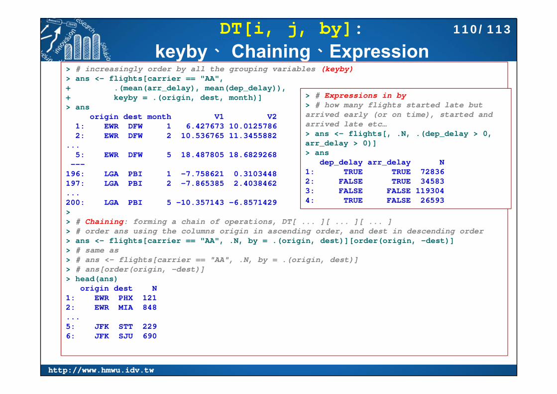
http://www.hmwu.idv.twhttp://www.hmwu.idv.tw
DT[i, j, by]:keyby、 Chaining、Expression
> # increasingly order by all the grouping variables (keyby)> ans <- flights[carrier == "AA",+ .(mean(arr_delay), mean(dep_delay)),+ keyby = .(origin, dest, month)]> ans
origin dest month V1 V21: EWR DFW 1 6.427673 10.01257862: EWR DFW 2 10.536765 11.3455882
...5: EWR DFW 5 18.487805 18.6829268
---196: LGA PBI 1 -7.758621 0.3103448197: LGA PBI 2 -7.865385 2.4038462...200: LGA PBI 5 -10.357143 -6.8571429> > # Chaining: forming a chain of operations, DT[ ... ][ ... ][ ... ]> # order ans using the columns origin in ascending order, and dest in descending order> ans <- flights[carrier == "AA", .N, by = .(origin, dest)][order(origin, -dest)]> # same as> # ans <- flights[carrier == "AA", .N, by = .(origin, dest)]> # ans[order(origin, -dest)]> head(ans)
origin dest N1: EWR PHX 1212: EWR MIA 848...5: JFK STT 2296: JFK SJU 690
> # Expressions in by> # how many flights started late but arrived early (or on time), started and arrived late etc…> ans <- flights[, .N, .(dep_delay > 0, arr_delay > 0)]> ans
dep_delay arr_delay N1: TRUE TRUE 728362: FALSE TRUE 345833: FALSE FALSE 1193044: TRUE FALSE 26593
110/113

http://www.hmwu.idv.twhttp://www.hmwu.idv.tw
DT[i, j, by]: .SD: Subset of Data
.SD: Subset of Data It by itself is a data.table that holds the data for the current group defined using
by. .SD contains all the columns except the grouping columns by default.
> DT <- data.table(ID = c("b", "b", "b", "a", "a", "c"), X1 = 1:6, X2 = 7:12, X3 = 13:18)
> DTID X1 X2 X3
1: b 1 7 132: b 2 8 143: b 3 9 154: a 4 10 165: a 5 11 176: c 6 12 18> DT[, print(.SD), by = ID]X1 X2 X3
1: 1 7 132: 2 8 143: 3 9 15
X1 X2 X31: 4 10 162: 5 11 17
X1 X2 X31: 6 12 18Empty data.table (0 rows) of 1 col: ID
> # compute means on multiple columns for each groups> DT[, lapply(.SD, mean), by = ID]
ID X1 X2 X31: b 2.0 8.0 14.02: a 4.5 10.5 16.53: c 6.0 12.0 18.0
> ans <- flights[, head(.SD, 2), by = month]> head(ans)
111/113

http://www.hmwu.idv.twhttp://www.hmwu.idv.tw
DT[i, j, by]: .SDcols: specify the columns
.SDcols: specify the columns e.g., .SDcols = c("arr_delay", "dep_delay") ensures that .SD contains only these two
columns for each group. - or !: remove columns colA:colB: select consecutive columns !(colA:colB) or -(colA:colB): deselect consecutive columns
> # compute the mean() of arr_delay and dep_delay columns grouped by origin, dest and month.> flights[carrier == "AA", # rows: Only on trips with carrier "AA"+ lapply(.SD, mean), # do: compute the mean+ by = .(origin, dest, month), # by: for every 'origin, dest, month'+ .SDcols = c("arr_delay", "dep_delay")] # for just those specified in .SDcols
origin dest month arr_delay dep_delay1: JFK LAX 1 6.590361 14.22891572: LGA PBI 1 -7.758621 0.31034483: EWR LAX 1 1.366667 7.50000004: JFK MIA 1 15.720670 18.74301685: JFK SEA 1 14.357143 30.7500000
---196: LGA MIA 10 -6.251799 -1.4208633197: JFK MIA 10 -1.880184 6.6774194198: EWR PHX 10 -3.032258 -4.2903226199: JFK MCO 10 -10.048387 -1.6129032200: JFK DCA 10 16.483871 15.5161290
112/113
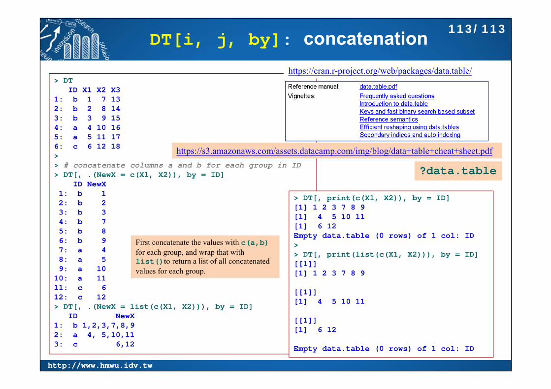
http://www.hmwu.idv.twhttp://www.hmwu.idv.tw
DT[i, j, by]: concatenation
> DTID X1 X2 X3
1: b 1 7 132: b 2 8 143: b 3 9 154: a 4 10 165: a 5 11 176: c 6 12 18>> # concatenate columns a and b for each group in ID> DT[, .(NewX = c(X1, X2)), by = ID]
ID NewX1: b 12: b 23: b 34: b 75: b 86: b 97: a 48: a 59: a 10
10: a 1111: c 612: c 12> DT[, .(NewX = list(c(X1, X2))), by = ID]
ID NewX1: b 1,2,3,7,8,92: a 4, 5,10,113: c 6,12
> DT[, print(c(X1, X2)), by = ID][1] 1 2 3 7 8 9[1] 4 5 10 11[1] 6 12Empty data.table (0 rows) of 1 col: ID> > DT[, print(list(c(X1, X2))), by = ID][[1]][1] 1 2 3 7 8 9
[[1]][1] 4 5 10 11
[[1]][1] 6 12
Empty data.table (0 rows) of 1 col: ID
First concatenate the values with c(a,b)for each group, and wrap that with list()to return a list of all concatenated values for each group.
https://cran.r-project.org/web/packages/data.table/
https://s3.amazonaws.com/assets.datacamp.com/img/blog/data+table+cheat+sheet.pdf
?data.table
113/113