Language Models Data-Intensive Information Processing Applications ! Session #6

Jordan Boyd-Graber University of Maryland

Thursday, March 10, 2011

This work is licensed under a Creative Commons Attribution-Noncommercial-Share Alike 3.0 United States See http://creativecommons.org/licenses/by-nc-sa/3.0/us/ for details

Source: Wikipedia (Japanese rock garden)

Today’s Agenda !  Sharing data and more complicated MR jobs

!  What are Language Models? "  Mathematical background and motivation "  Dealing with data sparsity (smoothing) "  Evaluating language models

!  Large Scale Language Models using MapReduce

!  Midterm

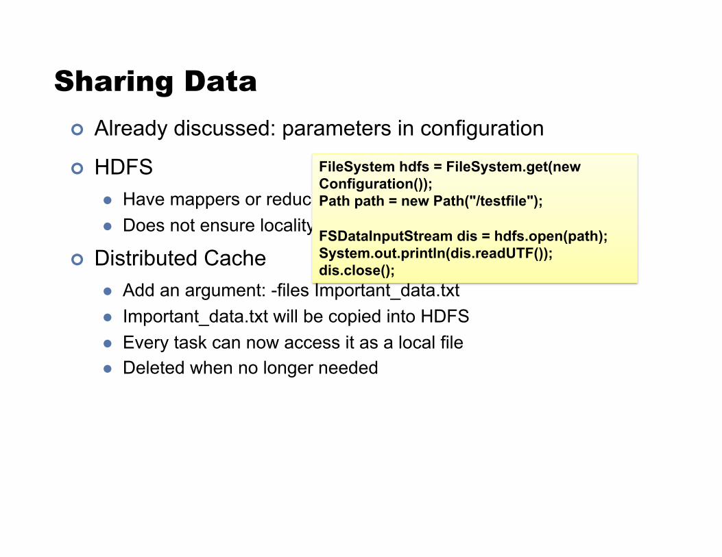
Sharing Data !  Already discussed: parameters in configuration

!  HDFS "  Have mappers or reducers open HDFS files "  Does not ensure locality

!  Distributed Cache "  Add an argument: -files Important_data.txt "  Important_data.txt will be copied into HDFS "  Every task can now access it as a local file "  Deleted when no longer needed

FileSystem hdfs = FileSystem.get(new Configuration()); Path path = new Path("/testfile");

FSDataInputStream dis = hdfs.open(path); System.out.println(dis.readUTF()); dis.close();

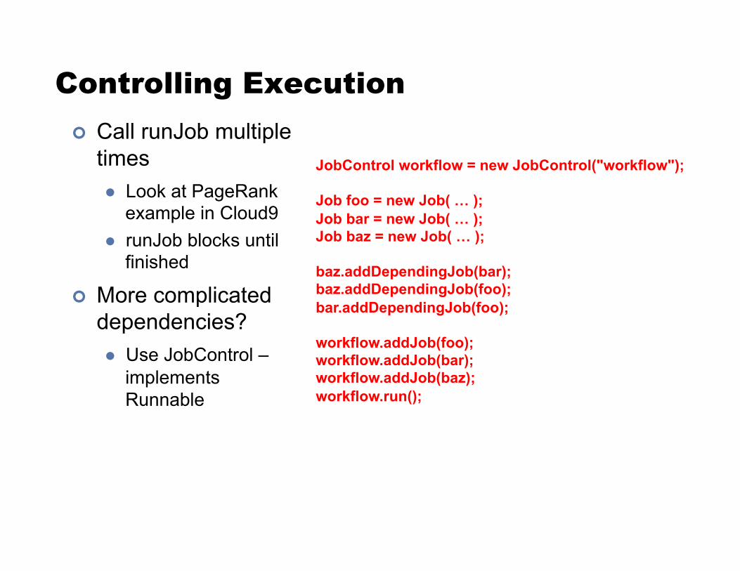
Controlling Execution !  Call runJob multiple

times "  Look at PageRank

example in Cloud9 "  runJob blocks until

finished

!  More complicated dependencies? "  Use JobControl –

implements Runnable

JobControl workflow = new JobControl("workflow");

Job foo = new Job( … ); Job bar = new Job( … ); Job baz = new Job( … );

baz.addDependingJob(bar); baz.addDependingJob(foo); bar.addDependingJob(foo);

workflow.addJob(foo); workflow.addJob(bar); workflow.addJob(baz); workflow.run();

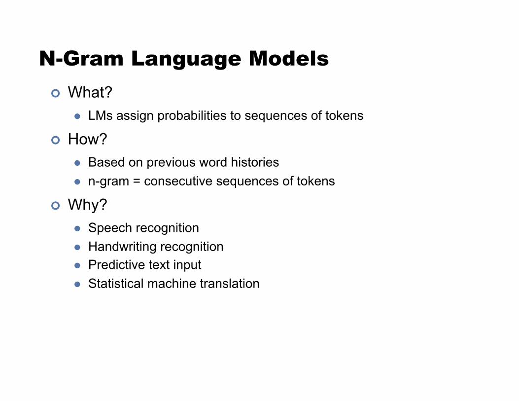
N-Gram Language Models !  What?

"  LMs assign probabilities to sequences of tokens

!  How? "  Based on previous word histories "  n-gram = consecutive sequences of tokens

!  Why? "  Speech recognition "  Handwriting recognition "  Predictive text input "  Statistical machine translation

i saw the small table vi la mesa pequeña

(vi, i saw) (la mesa pequeña, the small table) …

Parallel Sentences

Word Alignment Phrase Extraction

he sat at the table the service was good

Target-Language Text

Translation Model Language Model

Decoder

Foreign Input Sentence English Output Sentence

maria no daba una bofetada a la bruja verde mary did not slap the green witch

Training Data

Statistical Machine Translation

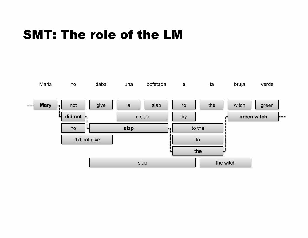
Maria no daba una bofetada a la bruja verde

Mary not

did not

no

did not give

give a slap to the witch green

slap

a slap

to the

to

the

green witch

the witch

by

slap

SMT: The role of the LM

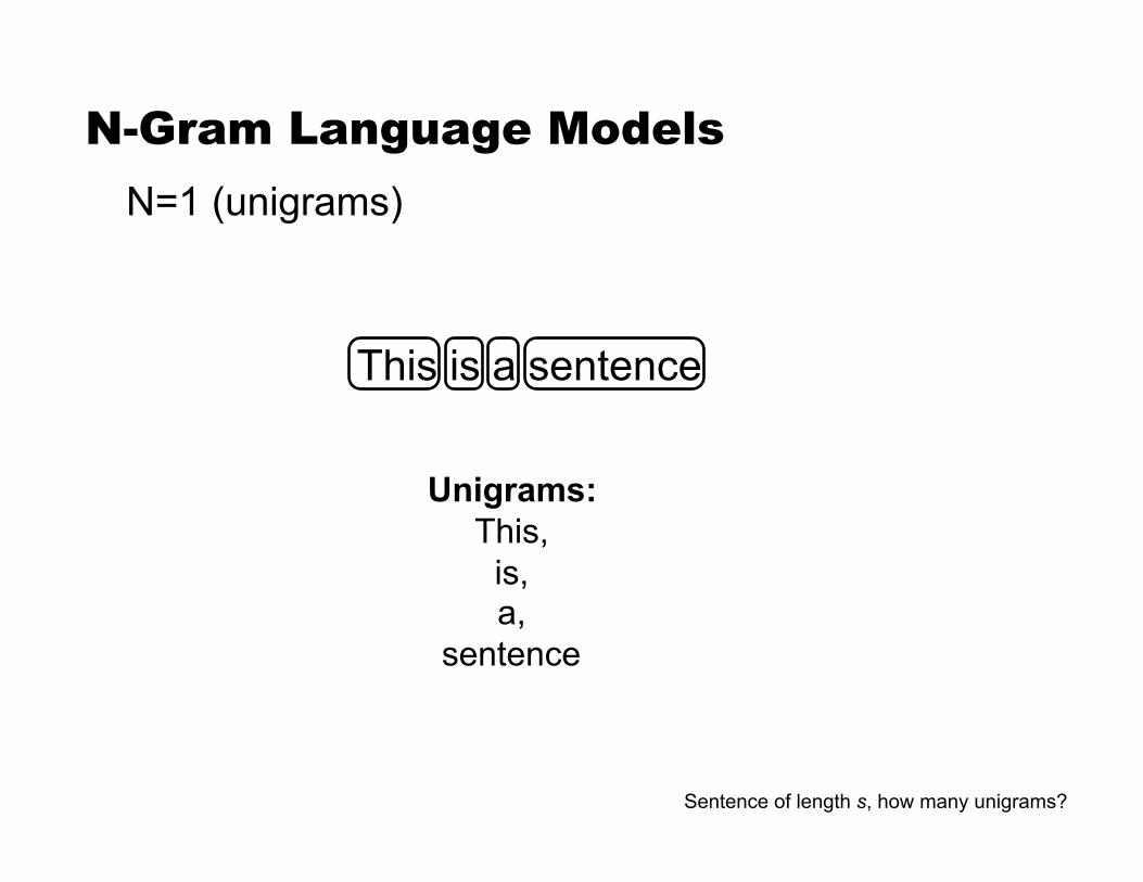
This is a sentence

N-Gram Language Models N=1 (unigrams)

Unigrams: This,

is, a,

sentence

Sentence of length s, how many unigrams?

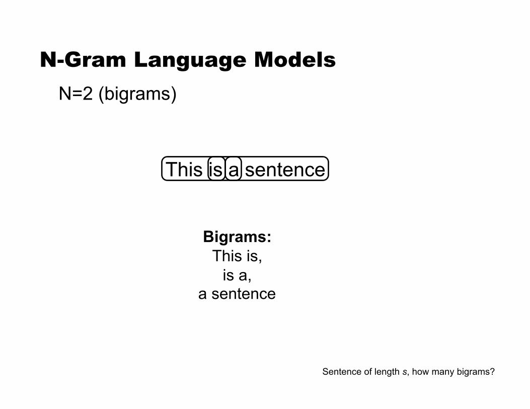
This is a sentence

N-Gram Language Models

Bigrams: This is,

is a, a sentence

N=2 (bigrams)

Sentence of length s, how many bigrams?

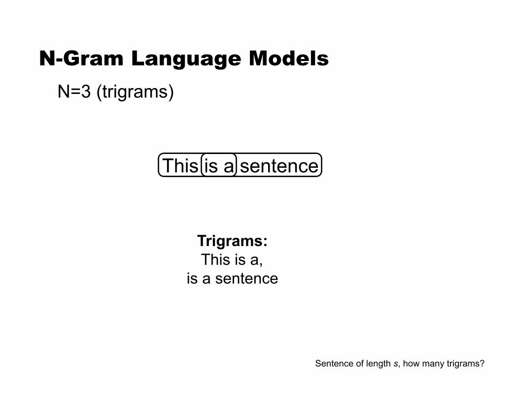
This is a sentence

N-Gram Language Models

Trigrams: This is a,

is a sentence

N=3 (trigrams)

Sentence of length s, how many trigrams?

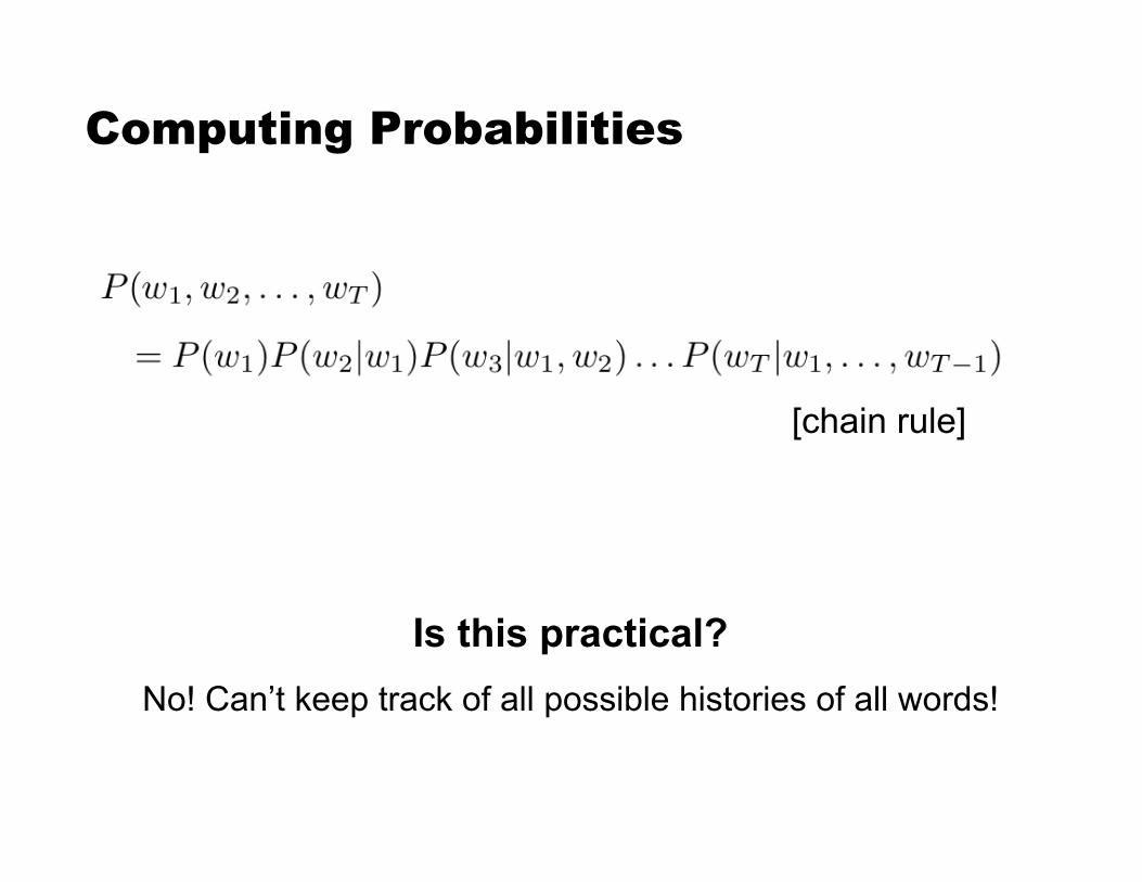
Computing Probabilities

Is this practical? No! Can’t keep track of all possible histories of all words!

[chain rule]

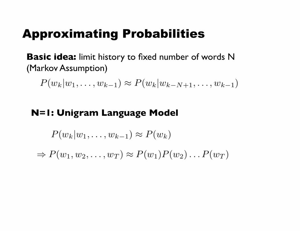
Approximating Probabilities

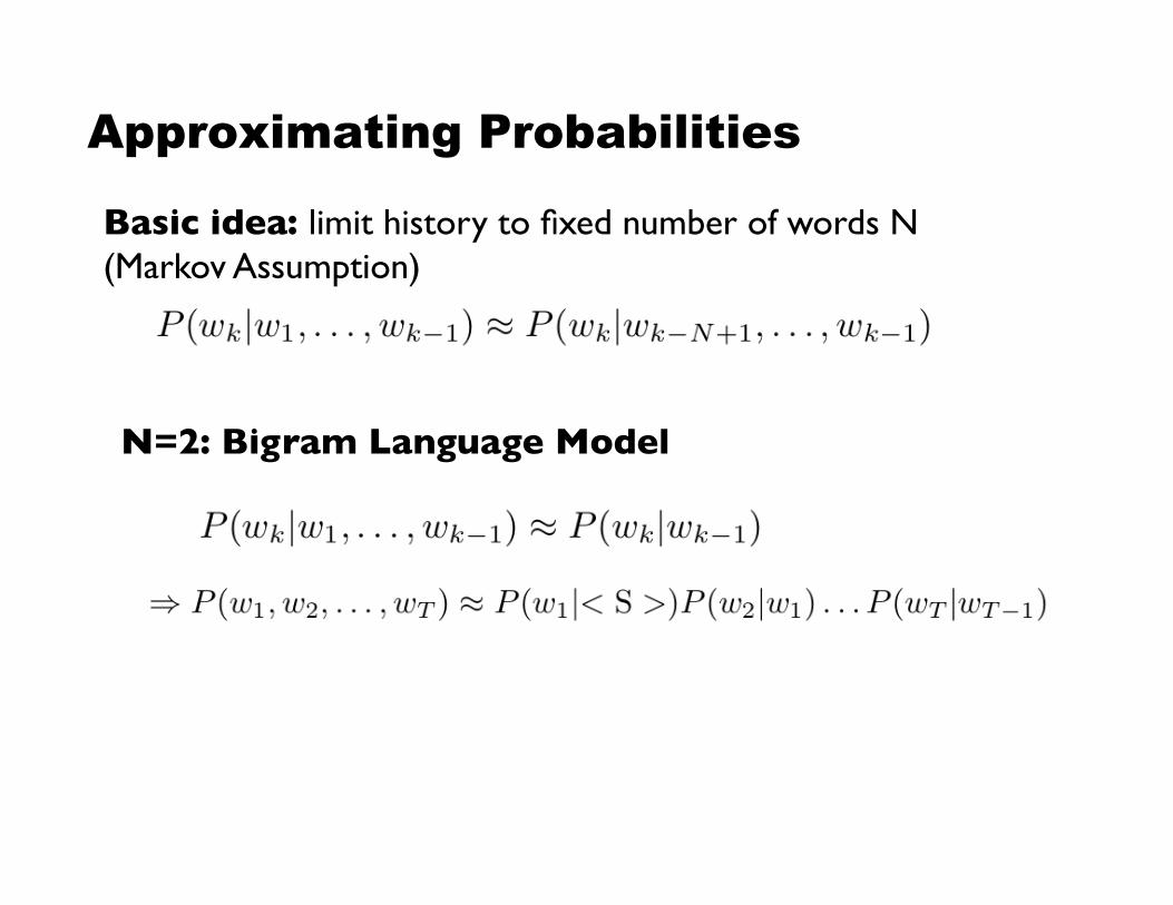
Basic idea: limit history to fixed number of words N!(Markov Assumption)!

N=1: Unigram Language Model!

Approximating Probabilities

Basic idea: limit history to fixed number of words N!(Markov Assumption)!

N=2: Bigram Language Model!

Approximating Probabilities

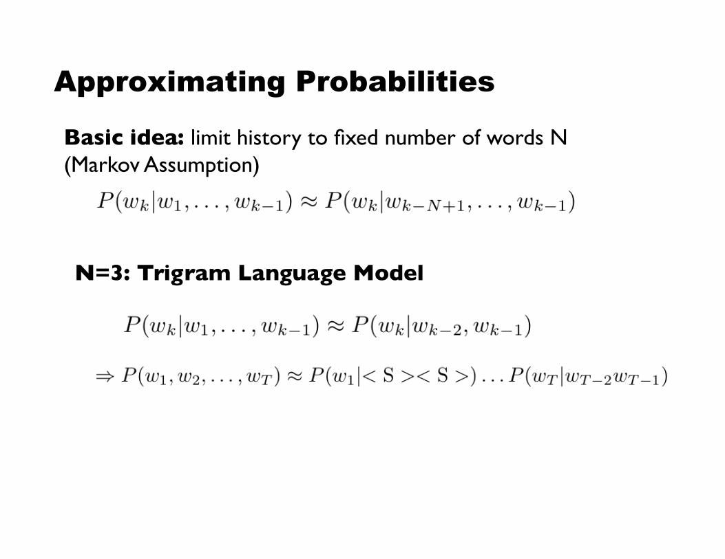
Basic idea: limit history to fixed number of words N!(Markov Assumption)!

N=3: Trigram Language Model!

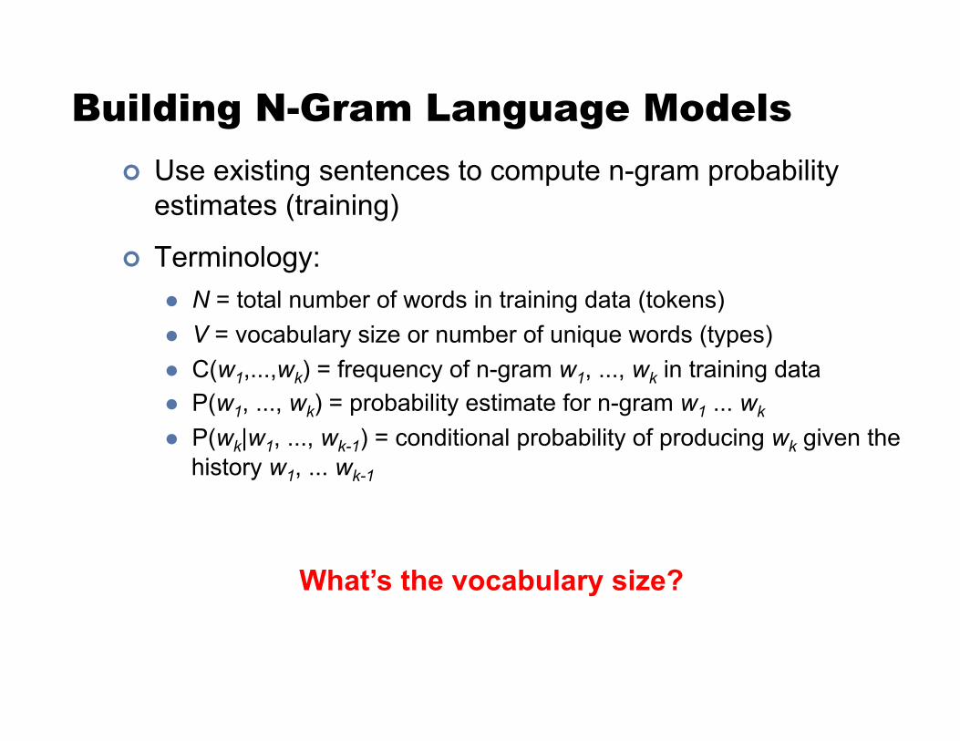
Building N-Gram Language Models !  Use existing sentences to compute n-gram probability

estimates (training)

!  Terminology: "  N = total number of words in training data (tokens) "  V = vocabulary size or number of unique words (types) "  C(w1,...,wk) = frequency of n-gram w1, ..., wk in training data "  P(w1, ..., wk) = probability estimate for n-gram w1 ... wk

"  P(wk|w1, ..., wk-1) = conditional probability of producing wk given the history w1, ... wk-1

What’s the vocabulary size?

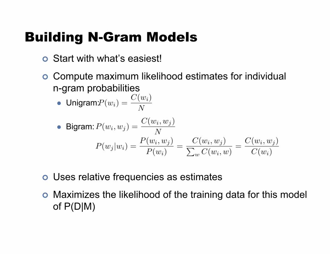
Building N-Gram Models !  Start with what’s easiest!

!  Compute maximum likelihood estimates for individual n-gram probabilities "  Unigram:

"  Bigram:

!  Uses relative frequencies as estimates

!  Maximizes the likelihood of the training data for this model of P(D|M)

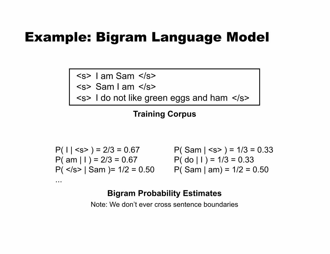
Example: Bigram Language Model

Note: We don’t ever cross sentence boundaries

I am Sam Sam I am I do not like green eggs and ham

<s> <s> <s>

</s> </s>

</s>

Training Corpus

P( I | <s> ) = 2/3 = 0.67 P( Sam | <s> ) = 1/3 = 0.33 P( am | I ) = 2/3 = 0.67 P( do | I ) = 1/3 = 0.33 P( </s> | Sam )= 1/2 = 0.50 P( Sam | am) = 1/2 = 0.50 ...

Bigram Probability Estimates

Building N-Gram Models !  Start with what’s easiest!

!  Compute maximum likelihood estimates for individual n-gram probabilities "  Unigram:

"  Bigram:

!  Uses relative frequencies as estimates

!  Maximizes the likelihood of the data given the model P(D|M)

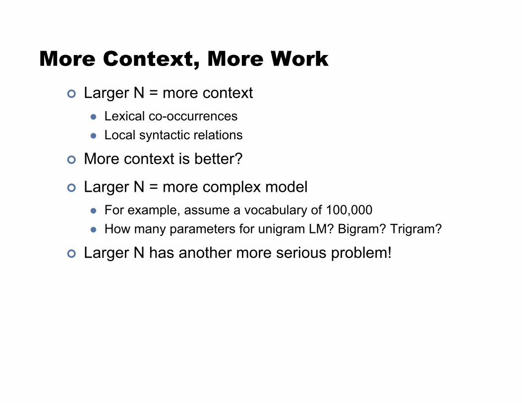
More Context, More Work !  Larger N = more context

"  Lexical co-occurrences "  Local syntactic relations

!  More context is better?

!  Larger N = more complex model "  For example, assume a vocabulary of 100,000 "  How many parameters for unigram LM? Bigram? Trigram?

!  Larger N has another more serious problem!

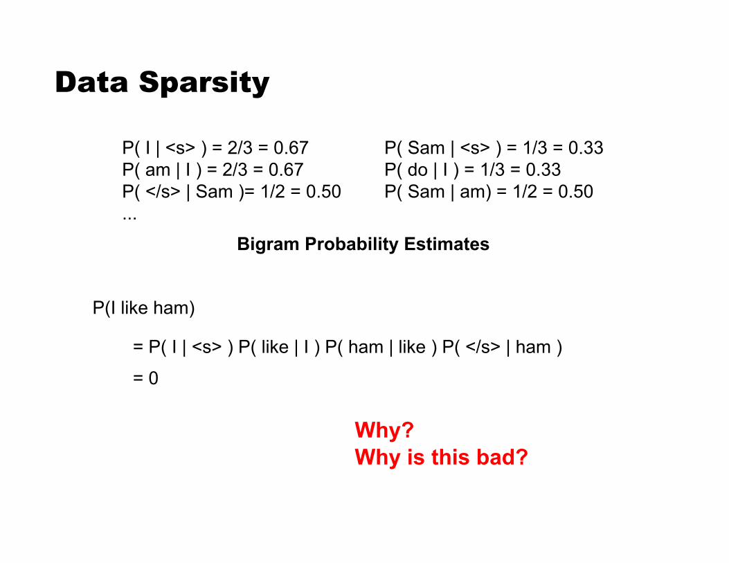
Data Sparsity

P(I like ham)

= P( I | <s> ) P( like | I ) P( ham | like ) P( </s> | ham )

= 0

P( I | <s> ) = 2/3 = 0.67 P( Sam | <s> ) = 1/3 = 0.33 P( am | I ) = 2/3 = 0.67 P( do | I ) = 1/3 = 0.33 P( </s> | Sam )= 1/2 = 0.50 P( Sam | am) = 1/2 = 0.50 ...

Bigram Probability Estimates

Why? Why is this bad?

Data Sparsity !  Serious problem in language modeling!

!  Becomes more severe as N increases "  What’s the tradeoff?

!  Solution 1: Use larger training corpora "  Can’t always work... Blame Zipf’s Law (Looong tail)

!  Solution 2: Assign non-zero probability to unseen n-grams "  Known as smoothing

Smoothing !  Zeros are bad for any statistical estimator

"  Need better estimators because MLEs give us a lot of zeros "  A distribution without zeros is “smoother”

!  The Robin Hood Philosophy: Take from the rich (seen n-grams) and give to the poor (unseen n-grams) "  And thus also called discounting "  Critical: make sure you still have a valid probability distribution!

!  Language modeling: theory vs. practice

Laplace’s Law !  Simplest and oldest smoothing technique

"  Statistical justification: Uniform prior over multinomial distributions

!  Just add 1 to all n-gram counts including the unseen ones

!  So, what do the revised estimates look like?

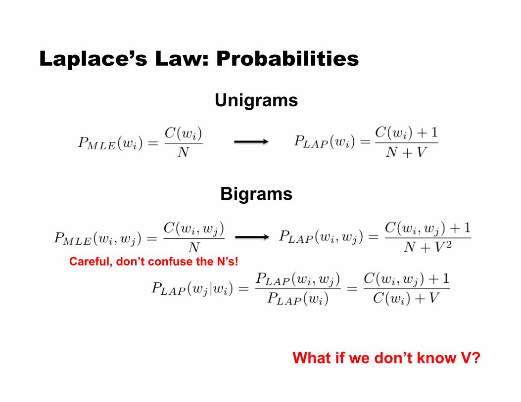
Laplace’s Law: Probabilities

Unigrams

Bigrams

What if we don’t know V?

Careful, don’t confuse the N’s!

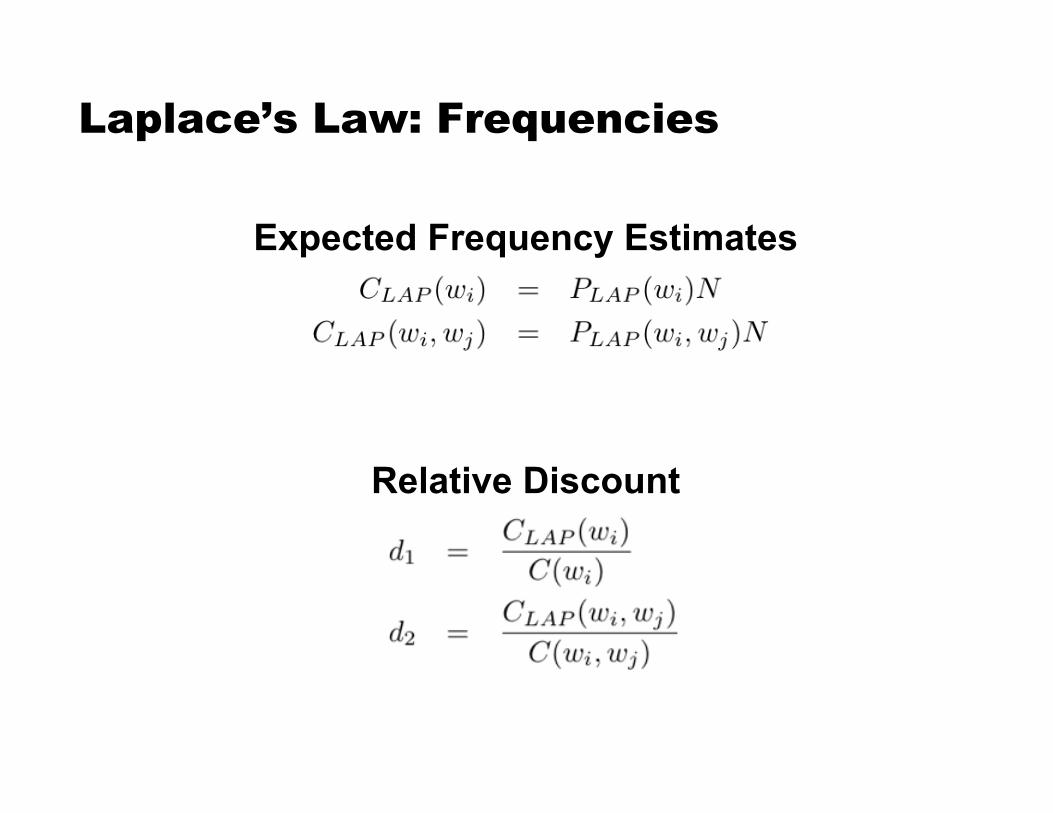
Laplace’s Law: Frequencies

Expected Frequency Estimates

Relative Discount

Laplace’s Law !  Bayesian estimator with uniform priors

!  Moves too much mass over to unseen n-grams

!  What if we added a fraction of 1 instead?

Lidstone’s Law of Succession !  Add 0 < ! < 1 to each count instead

!  The smaller ! is, the lower the mass moved to the unseen n-grams (0=no smoothing)

!  The case of ! = 0.5 is known as Jeffery-Perks Law or Expected Likelihood Estimation

!  How to find the right value of !?

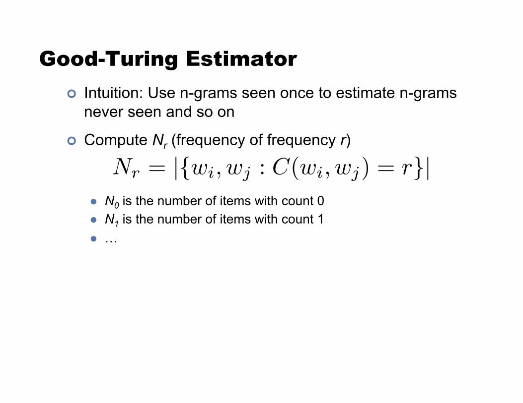
Good-Turing Estimator !  Intuition: Use n-grams seen once to estimate n-grams

never seen and so on

!  Compute Nr (frequency of frequency r)

"  N0 is the number of items with count 0 "  N1 is the number of items with count 1 "  …

Nr = |{wi, wj : C(wi, wj) = r}|

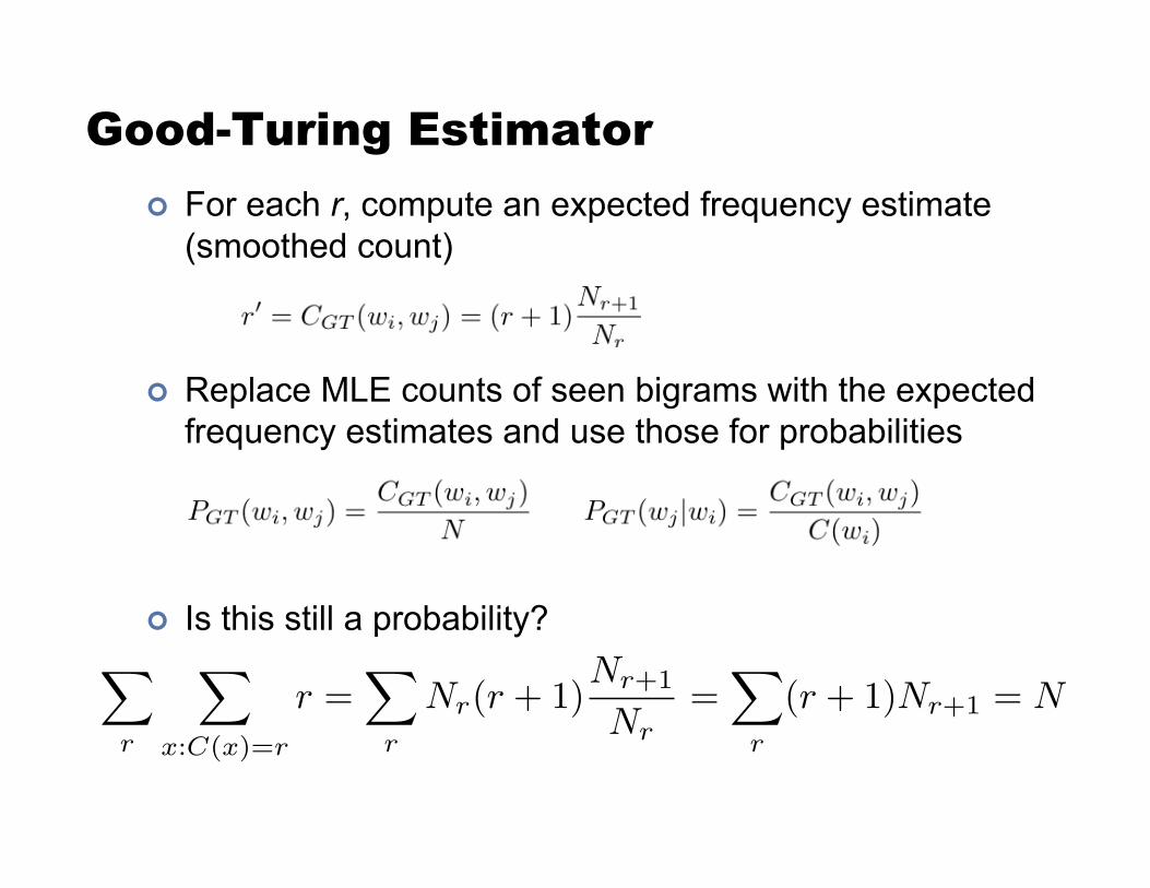
Good-Turing Estimator !  For each r, compute an expected frequency estimate

(smoothed count)

!  Replace MLE counts of seen bigrams with the expected frequency estimates and use those for probabilities

!  Is this still a probability? �

r

�

x:C(x)=r

r =�

r

Nr(r + 1)Nr+1

Nr=

�

r

(r + 1)Nr+1 = N

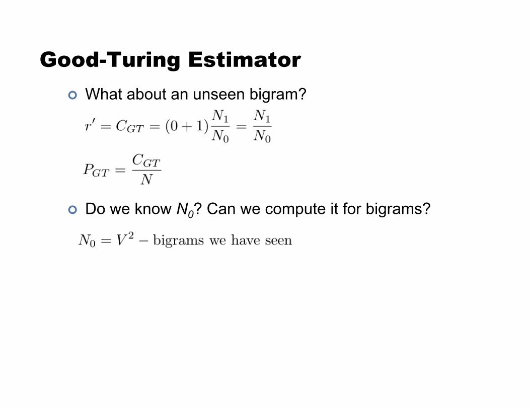
Good-Turing Estimator !  What about an unseen bigram?

!  Do we know N0? Can we compute it for bigrams?

Good-Turing Estimator: Example

r! Nr!

1! 138741!

2! 25413!

3! 10531!

4! 5997!

5! 3565!

6! ...!

V = 14585 Seen bigrams =199252

C(person she) = 2 C(person) = 223

(14585)2 - 199252

N1 / N0 = 0.00065 N1 /( N0 N ) = 1.06 x 10-9

N0 =

Cunseen = Punseen =

CGT(person she) = (2+1)(10531/25413) = 1.243 P(she|person) =CGT(person she)/223 = 0.0056

Note: Assumes mass is uniformly distributed

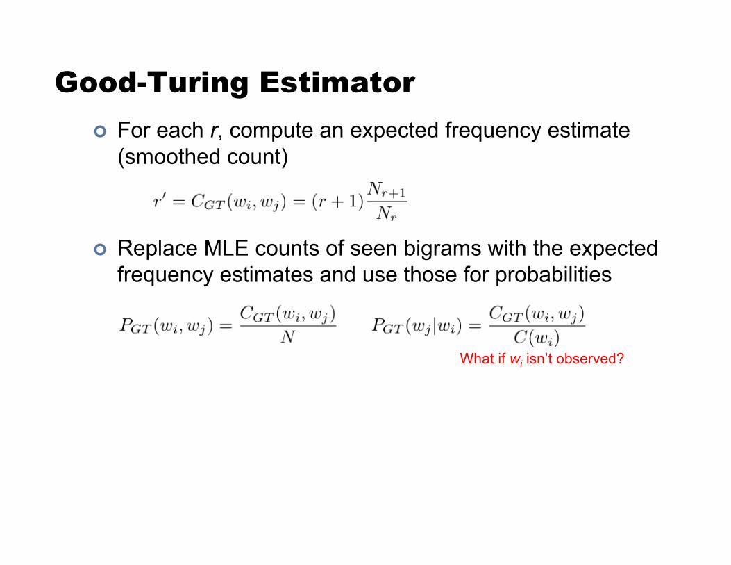
Good-Turing Estimator !  For each r, compute an expected frequency estimate

(smoothed count)

!  Replace MLE counts of seen bigrams with the expected frequency estimates and use those for probabilities

What if wi isn’t observed?

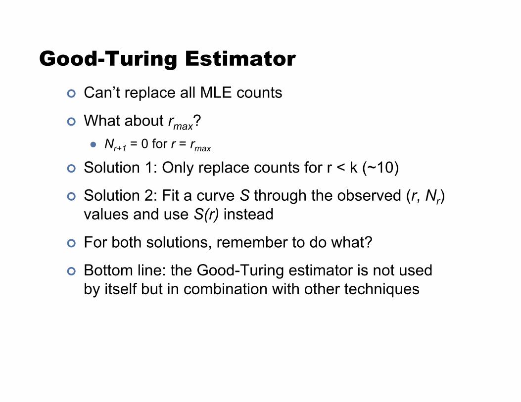
Good-Turing Estimator !  Can’t replace all MLE counts

!  What about rmax? "  Nr+1 = 0 for r = rmax

!  Solution 1: Only replace counts for r < k (~10)

!  Solution 2: Fit a curve S through the observed (r, Nr) values and use S(r) instead

!  For both solutions, remember to do what?

!  Bottom line: the Good-Turing estimator is not used by itself but in combination with other techniques

Combining Estimators !  Better models come from:

"  Combining n-gram probability estimates from different models "  Leveraging different sources of information for prediction

!  Three major combination techniques: "  Simple Linear Interpolation of MLEs "  Katz Backoff "  Kneser-Ney Smoothing

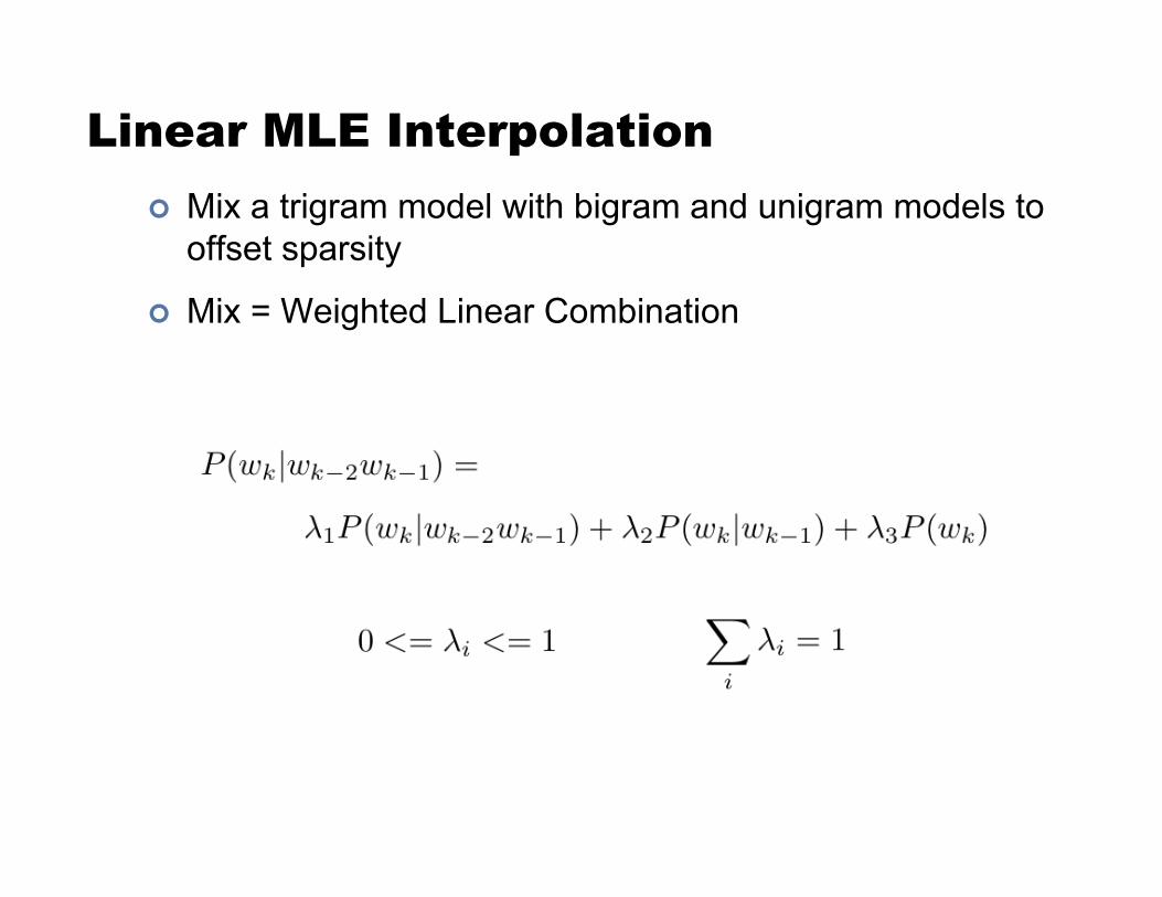
Linear MLE Interpolation !  Mix a trigram model with bigram and unigram models to

offset sparsity

!  Mix = Weighted Linear Combination

Linear MLE Interpolation !  !i are estimated on some held-out data set (not training,

not test)

!  Estimation is usually done via an EM variant or other numerical algorithms (e.g. Powell)

Backoff Models !  Consult different models in order depending on specificity

(instead of all at the same time)

!  The most detailed model for current context first and, if that doesn’t work, back off to a lower model

!  Continue backing off until you reach a model that has some counts

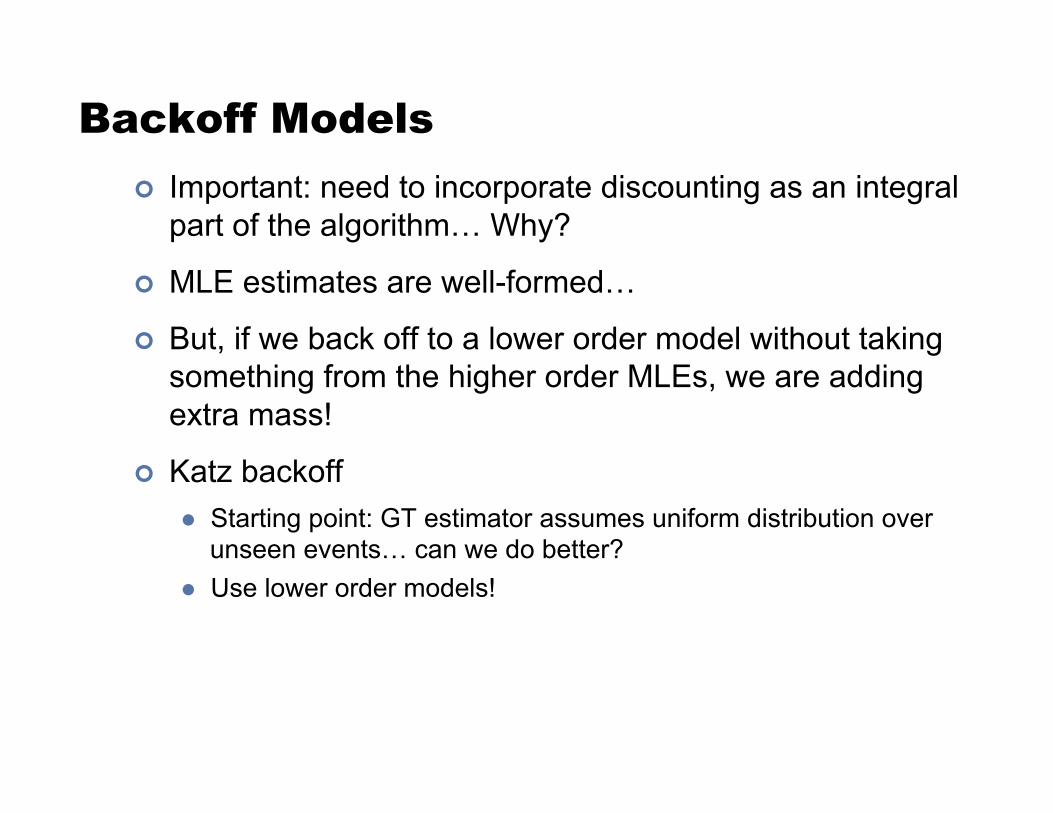
Backoff Models !  Important: need to incorporate discounting as an integral

part of the algorithm… Why?

!  MLE estimates are well-formed…

!  But, if we back off to a lower order model without taking something from the higher order MLEs, we are adding extra mass!

!  Katz backoff "  Starting point: GT estimator assumes uniform distribution over

unseen events… can we do better? "  Use lower order models!

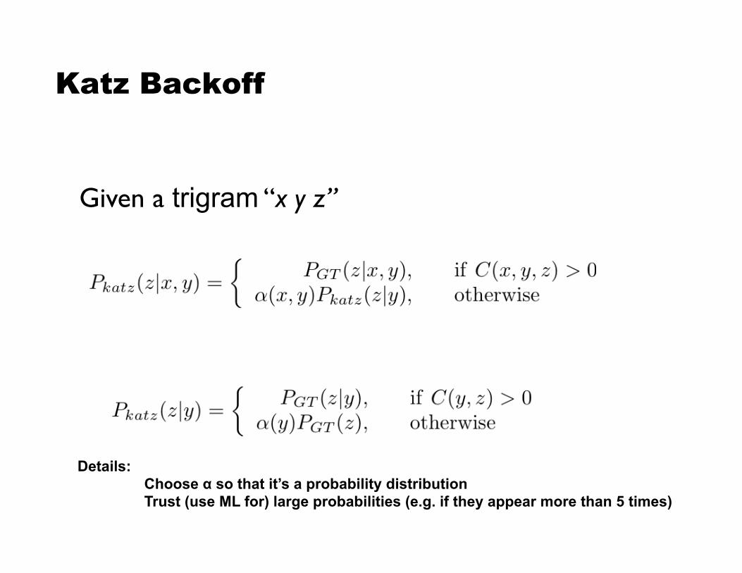
Katz Backoff

Given a trigram “x y z”!

Details: Choose " so that it’s a probability distribution Trust (use ML for) large probabilities (e.g. if they appear more than 5 times)

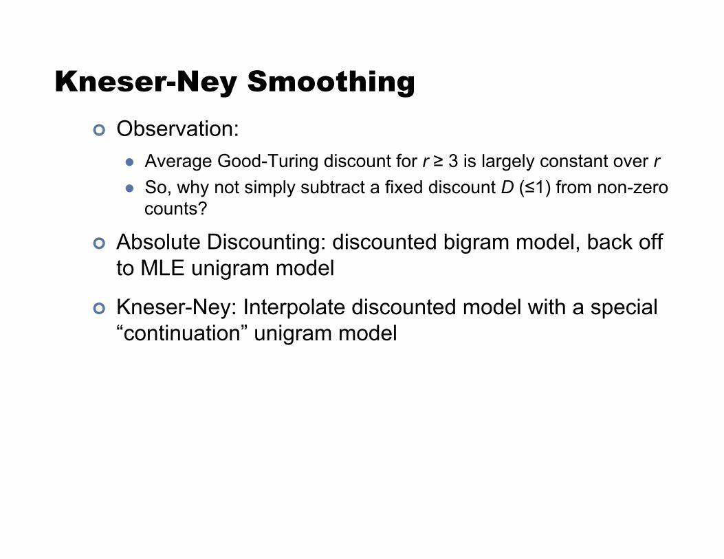
Kneser-Ney Smoothing !  Observation:

"  Average Good-Turing discount for r " 3 is largely constant over r "  So, why not simply subtract a fixed discount D (#1) from non-zero

counts?

!  Absolute Discounting: discounted bigram model, back off to MLE unigram model

!  Kneser-Ney: Interpolate discounted model with a special “continuation” unigram model

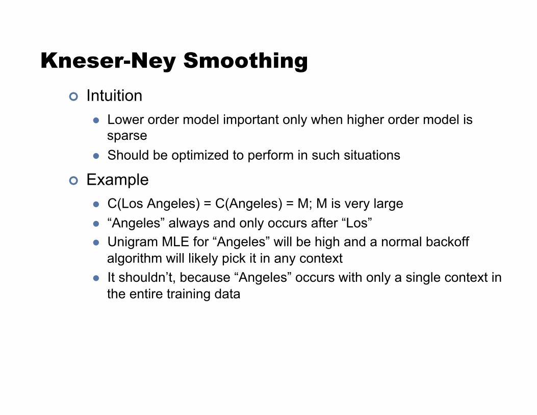
Kneser-Ney Smoothing !  Intuition

"  Lower order model important only when higher order model is sparse

"  Should be optimized to perform in such situations

!  Example "  C(Los Angeles) = C(Angeles) = M; M is very large "  “Angeles” always and only occurs after “Los” "  Unigram MLE for “Angeles” will be high and a normal backoff

algorithm will likely pick it in any context "  It shouldn’t, because “Angeles” occurs with only a single context in

the entire training data

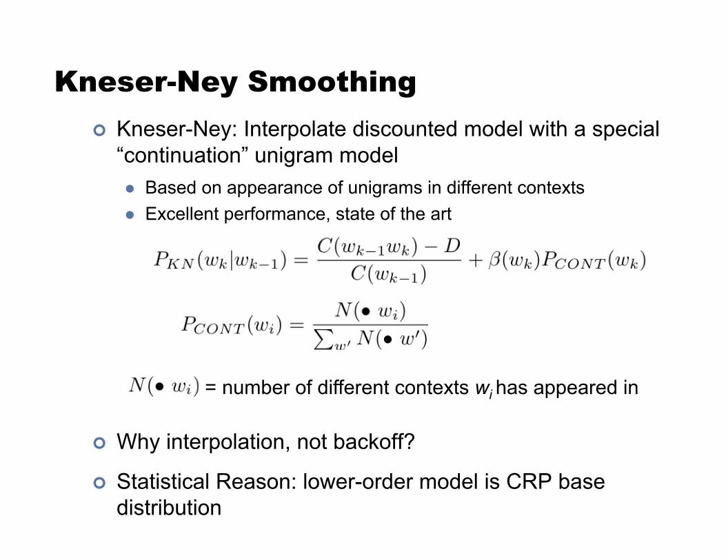
Kneser-Ney Smoothing !  Kneser-Ney: Interpolate discounted model with a special

“continuation” unigram model "  Based on appearance of unigrams in different contexts "  Excellent performance, state of the art

!  Why interpolation, not backoff?

!  Statistical Reason: lower-order model is CRP base distribution

= number of different contexts wi has appeared in

Explicitly Modeling OOV !  Fix vocabulary at some reasonable number of words

!  During training: "  Consider any words that don’t occur in this list as unknown or out

of vocabulary (OOV) words "  Replace all OOVs with the special word <UNK> "  Treat <UNK> as any other word and count and estimate

probabilities

!  During testing: "  Replace unknown words with <UNK> and use LM "  Test set characterized by OOV rate (percentage of OOVs)

Evaluating Language Models !  Information theoretic criteria used

!  Most common: Perplexity assigned by the trained LM to a test set

!  Perplexity: How surprised are you on average by what comes next ? "  If the LM is good at knowing what comes next in a sentence ⇒

Low perplexity (lower is better) "  Relation to weighted average branching factor

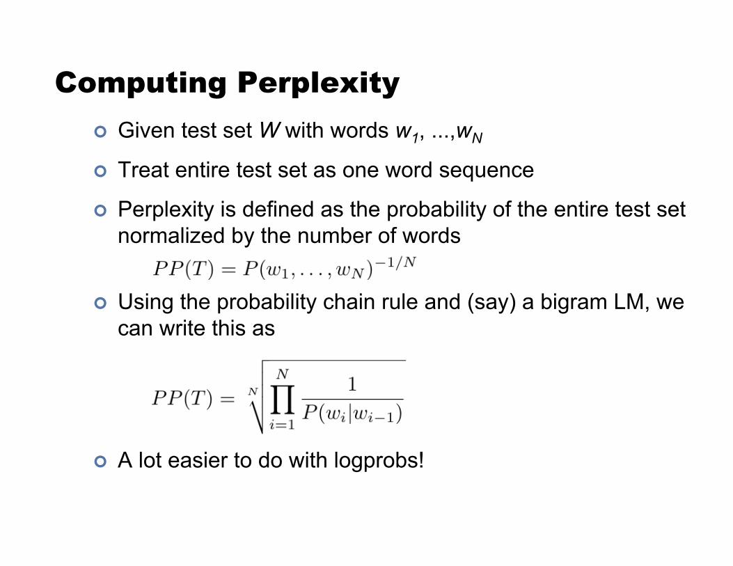
Computing Perplexity !  Given test set W with words w1, ...,wN

!  Treat entire test set as one word sequence

!  Perplexity is defined as the probability of the entire test set normalized by the number of words

!  Using the probability chain rule and (say) a bigram LM, we can write this as

!  A lot easier to do with logprobs!

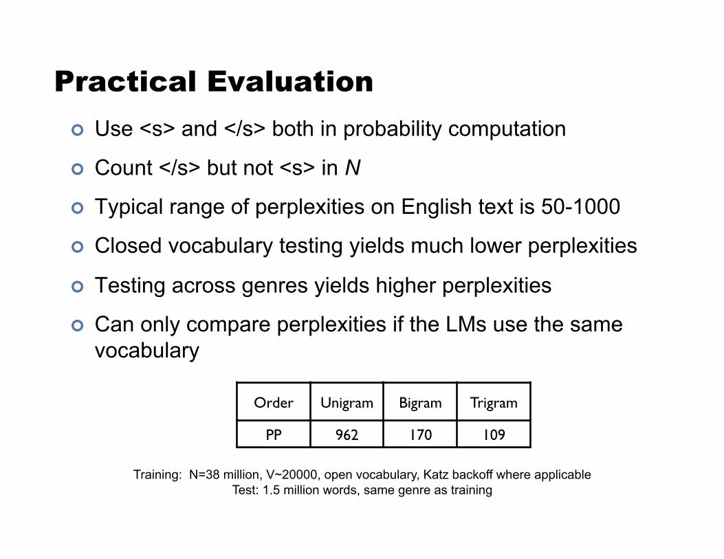
Practical Evaluation !  Use <s> and </s> both in probability computation

!  Count </s> but not <s> in N

!  Typical range of perplexities on English text is 50-1000

!  Closed vocabulary testing yields much lower perplexities

!  Testing across genres yields higher perplexities

!  Can only compare perplexities if the LMs use the same vocabulary

Training: N=38 million, V~20000, open vocabulary, Katz backoff where applicable Test: 1.5 million words, same genre as training

Order! Unigram! Bigram! Trigram!

PP! 962! 170! 109!

Typical “State of the Art” LMs !  Training

"  N = 10 billion words, V = 300k words "  4-gram model with Kneser-Ney smoothing

!  Testing "  25 million words, OOV rate 3.8% "  Perplexity ~50

Take-Away Messages !  LMs assign probabilities to sequences of tokens

!  N-gram language models: consider only limited histories

!  Data sparsity is an issue: smoothing to the rescue "  Variations on a theme: different techniques for redistributing

probability mass "  Important: make sure you still have a valid probability distribution!

Scaling Language Models with

MapReduce

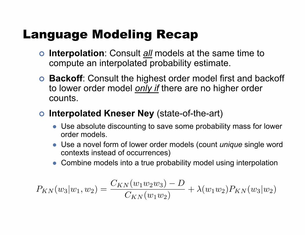
Language Modeling Recap !  Interpolation: Consult all models at the same time to

compute an interpolated probability estimate.

!  Backoff: Consult the highest order model first and backoff to lower order model only if there are no higher order counts.

!  Interpolated Kneser Ney (state-of-the-art) "  Use absolute discounting to save some probability mass for lower

order models. "  Use a novel form of lower order models (count unique single word

contexts instead of occurrences) "  Combine models into a true probability model using interpolation

Questions for today

Can we efficiently train an IKN LM with terabytes of data?

Does it really matter?

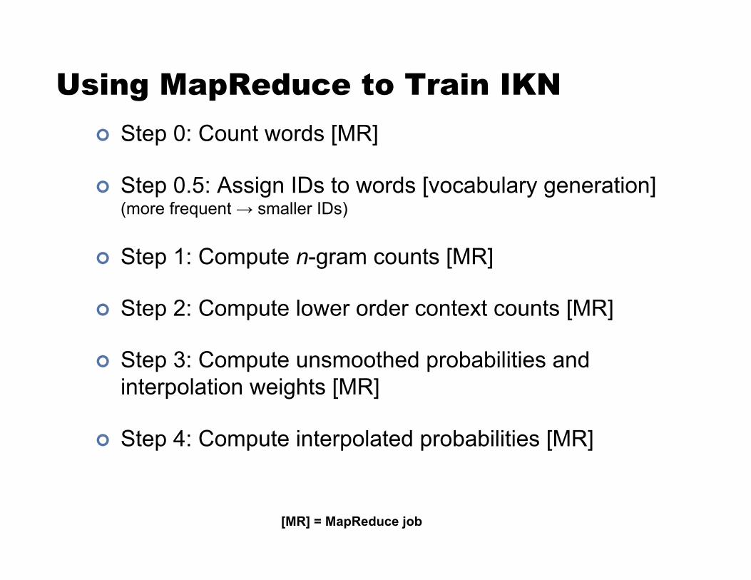
Using MapReduce to Train IKN !  Step 0: Count words [MR]

!  Step 0.5: Assign IDs to words [vocabulary generation] (more frequent $ smaller IDs)

!  Step 1: Compute n-gram counts [MR]

!  Step 2: Compute lower order context counts [MR]

!  Step 3: Compute unsmoothed probabilities and interpolation weights [MR]

!  Step 4: Compute interpolated probabilities [MR]

[MR] = MapReduce job

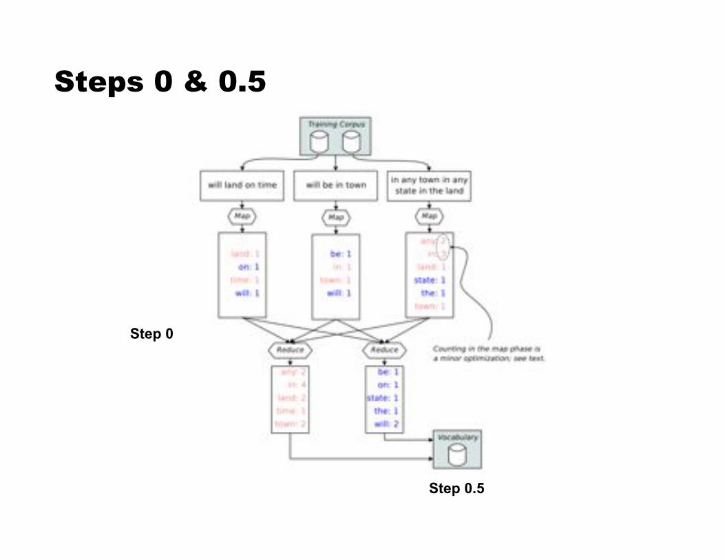
Steps 0 & 0.5

Step 0.5

Step 0

Steps 1-4 Step 1 Step 2 Step 3 Step 4

Input Key DocID n-grams “a b c” “a b c” “a b”

Input Value Document Ctotal(“a b c”) CKN(“a b c”) _Step 3 Output_

Intermediate Key

n-grams “a b c” “a b c” “a b” (history) “c b a”

Intermediate Value Cdoc(“a b c”) C’KN(“a b c”) (“c”, CKN(“a b c”)) (P’(“a b c”), %(“a b”))

Partitioning “a b c” “a b c” “a b” “c b”

Output Value Ctotal(“a b c”) CKN(“a b c”) (“c”, P’(“a b c”), %(“a b”))

(PKN(“a b c”), %(“a b”))

Count n-grams

All output keys are always the same as the intermediate keys I only show trigrams here but the steps operate on bigrams and unigrams as well

Count contexts

Compute unsmoothed probs AND interp. weights

Compute Interp. probs

Map

per I

nput

M

appe

r Out

put

Red

ucer

Inpu

t R

educ

er

Out

put

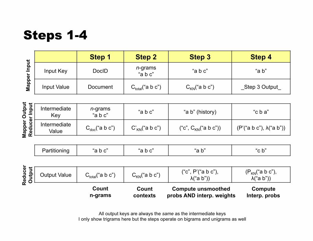
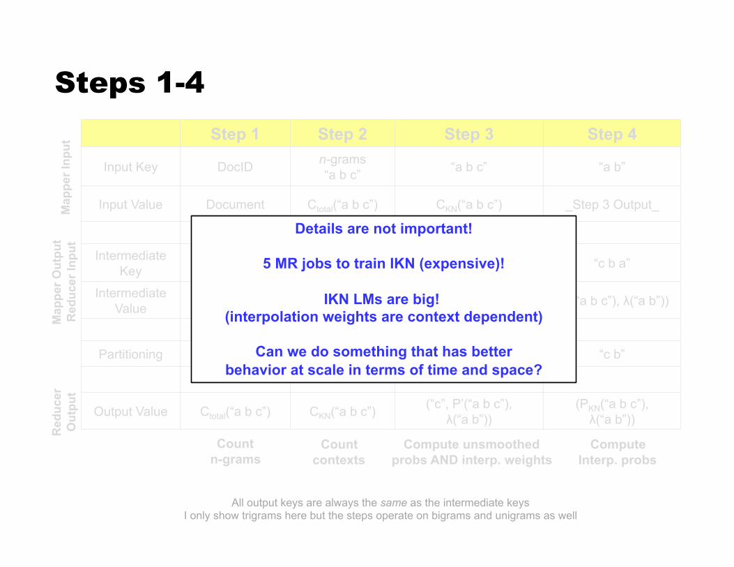
Steps 1-4 Step 1 Step 2 Step 3 Step 4

Input Key DocID n-grams “a b c” “a b c” “a b”

Input Value Document Ctotal(“a b c”) CKN(“a b c”) _Step 3 Output_

Intermediate Key

n-grams “a b c” “a b c” “a b” (history) “c b a”

Intermediate Value Cdoc(“a b c”) C’KN(“a b c”) (“c”, CKN(“a b c”)) (P’(“a b c”), %(“a b”))

Partitioning “a b c” “a b c” “a b” “c b”

Output Value Ctotal(“a b c”) CKN(“a b c”) (“c”, P’(“a b c”), %(“a b”))

(PKN(“a b c”), %(“a b”))

Count n-grams

All output keys are always the same as the intermediate keys I only show trigrams here but the steps operate on bigrams and unigrams as well

Count contexts

Compute unsmoothed probs AND interp. weights

Compute Interp. probs

Map

per I

nput

M

appe

r Out

put

Red

ucer

Inpu

t R

educ

er

Out

put

Details are not important!

5 MR jobs to train IKN (expensive)!

IKN LMs are big! (interpolation weights are context dependent)

Can we do something that has better behavior at scale in terms of time and space?

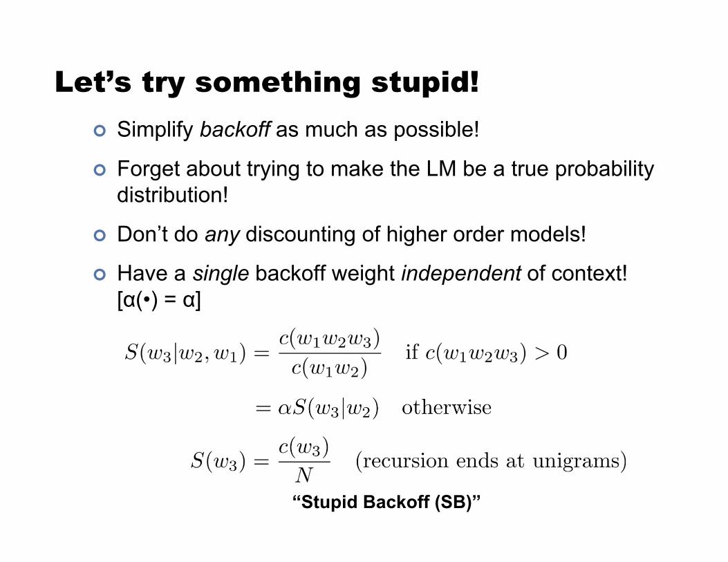
Let’s try something stupid! !  Simplify backoff as much as possible!

!  Forget about trying to make the LM be a true probability distribution!

!  Don’t do any discounting of higher order models!

!  Have a single backoff weight independent of context! [&(•) = &]

“Stupid Backoff (SB)”

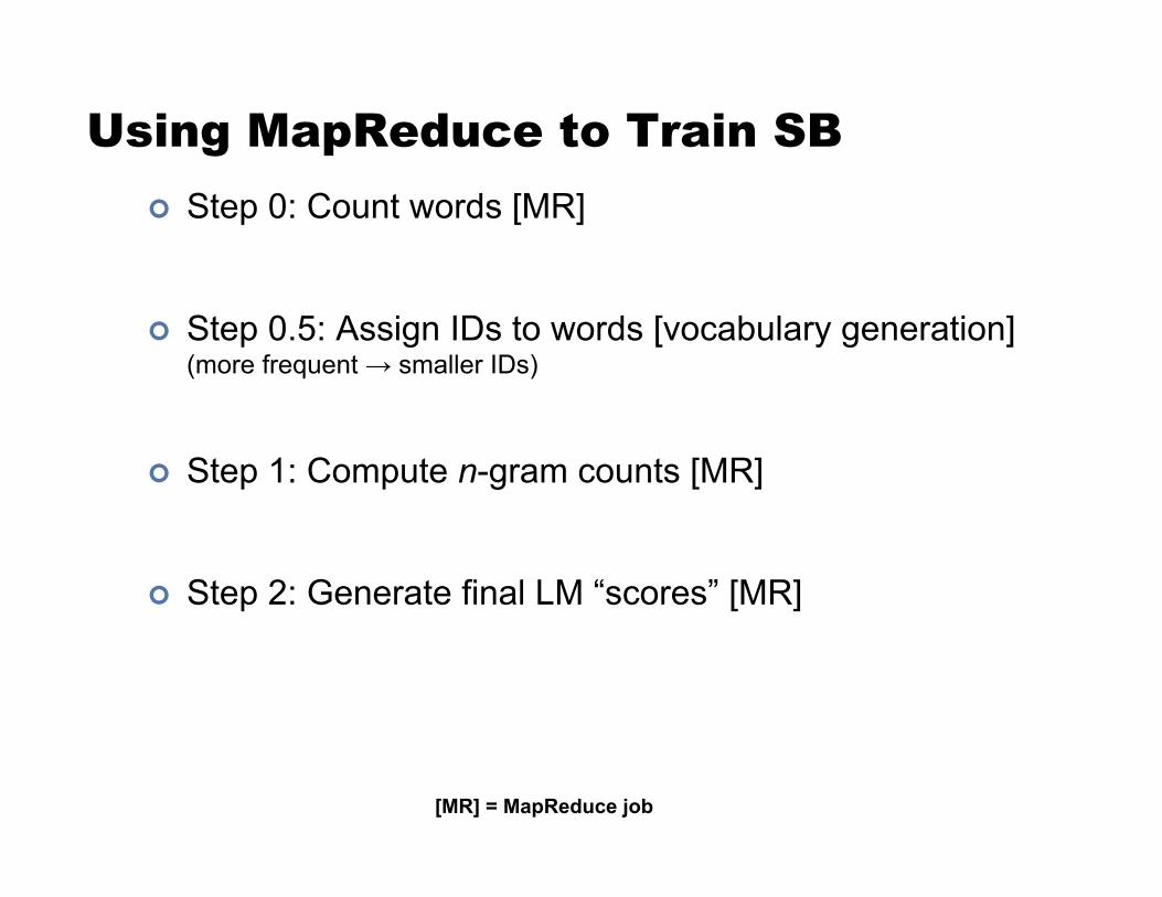
Using MapReduce to Train SB !  Step 0: Count words [MR]

!  Step 0.5: Assign IDs to words [vocabulary generation] (more frequent $ smaller IDs)

!  Step 1: Compute n-gram counts [MR]

!  Step 2: Generate final LM “scores” [MR]

[MR] = MapReduce job

Steps 0 & 0.5

Step 0.5

Step 0

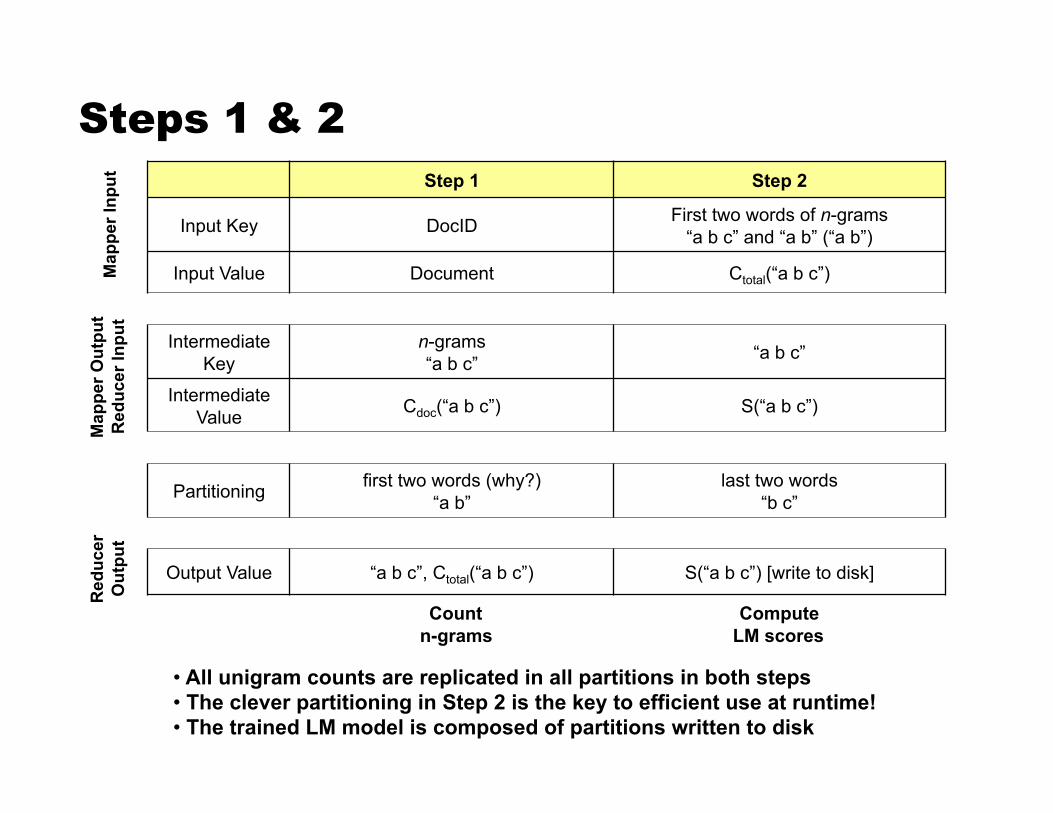
Steps 1 & 2 Step 1 Step 2

Input Key DocID First two words of n-grams “a b c” and “a b” (“a b”)

Input Value Document Ctotal(“a b c”)

Intermediate Key

n-grams “a b c” “a b c”

Intermediate Value Cdoc(“a b c”) S(“a b c”)

Partitioning first two words (why?) “a b”

last two words “b c”

Output Value “a b c”, Ctotal(“a b c”) S(“a b c”) [write to disk]

Count n-grams

Compute LM scores

•  All unigram counts are replicated in all partitions in both steps •  The clever partitioning in Step 2 is the key to efficient use at runtime!

•  The trained LM model is composed of partitions written to disk

Map

per I

nput

M

appe

r Out

put

Red

ucer

Inpu

t R

educ

er

Out

put

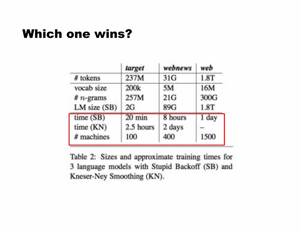
Which one wins?

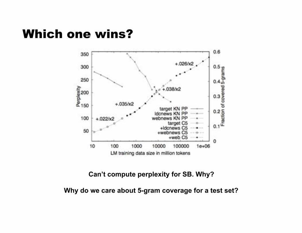
Which one wins?

Can’t compute perplexity for SB. Why?

Why do we care about 5-gram coverage for a test set?

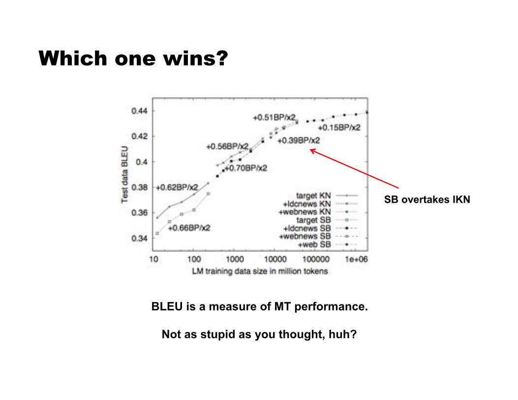
Which one wins?

BLEU is a measure of MT performance.

Not as stupid as you thought, huh?

SB overtakes IKN

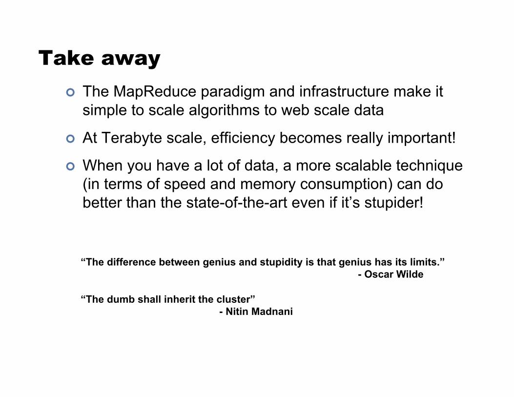
Take away !  The MapReduce paradigm and infrastructure make it

simple to scale algorithms to web scale data

!  At Terabyte scale, efficiency becomes really important!

!  When you have a lot of data, a more scalable technique (in terms of speed and memory consumption) can do better than the state-of-the-art even if it’s stupider!

“The difference between genius and stupidity is that genius has its limits.” - Oscar Wilde

“The dumb shall inherit the cluster” - Nitin Madnani

Midterm !  30-50 Multiple Choice Questions

"  Basic concepts "  Not particularly hard or tricky "  Intersection of lecture and readings

!  2-3 Free Response Questions "  Write a psedocode MapReduce program to … "  Simulate this algorithm on simple input

!  Have all of class, shouldn’t take more than an hour

!  Sample questions …

Source: Wikipedia (Japanese rock garden)

Questions?