· data ground-collected invasive plant data the usda forest inventory and analysis (fia) program...
TRANSCRIPT

1 23
Landscape Ecology ISSN 0921-2973Volume 31Number 1 Landscape Ecol (2016) 31:67-84DOI 10.1007/s10980-015-0295-0
Data, data everywhere: detecting spatialpatterns in fine-scale ecological informationcollected across a continent
Kevin M. Potter, Frank H. Koch,Christopher M. Oswalt & BasilV. Iannone

1 23
Your article is protected by copyright and all
rights are held exclusively by Springer Science
+Business Media Dordrecht. This e-offprint
is for personal use only and shall not be self-
archived in electronic repositories. If you wish
to self-archive your article, please use the
accepted manuscript version for posting on
your own website. You may further deposit
the accepted manuscript version in any
repository, provided it is only made publicly
available 12 months after official publication
or later and provided acknowledgement is
given to the original source of publication
and a link is inserted to the published article
on Springer's website. The link must be
accompanied by the following text: "The final
publication is available at link.springer.com”.

RESEARCH ARTICLE
Data, data everywhere: detecting spatial patterns in fine-scale ecological information collected across a continent
Kevin M. Potter . Frank H. Koch .
Christopher M. Oswalt . Basil V. Iannone III
Received: 25 May 2015 / Accepted: 28 September 2015 / Published online: 6 October 2015
� Springer Science+Business Media Dordrecht 2015
Abstract
Context Fine-scale ecological data collected across
broad regions are becoming increasingly available.
Appropriate geographic analyses of these data can
help identify locations of ecological concern.
Objectives We present one such approach, spatial
association of scalable hexagons (SASH), which
identifies locations where ecological phenomena
occur at greater or lower frequencies than expected
by chance. This approach is based on a sampling frame
optimized for spatial neighborhood analysis,
adjustable to the appropriate spatial resolution, and
applicable to multiple data types.
Methods We divided portions of the United States
into scalable equal-area hexagonal cells and, using
three types of data (field surveys, aerial surveys,
satellite imagery), identified geographic clusters of
forested areas having high and low values for (1)
invasive plant diversity and cover, (2) mountain pine
beetle-induced tree mortality, and (3) wildland forest
fire occurrences.
Results Using the SASH approach, we detected
statistically significant patterns of plant invasion, bark
beetle-induced tree mortality, and fire occurrence
density that will be useful for understanding macro-
scale patterns and processes associated with each
forest health threat, for assessing its ecological and
economic impacts, and for identifying areas where
specific management activities may be needed.
Conclusions The presented method is a ‘‘big data’’
analysis tool with potential application for macrosys-
tems ecology studies that require rigorous testing of
hypotheses within a spatial framework. This method is
a standard component of annual national reports on
Special issue: Macrosystems ecology: Novel methods and new
understanding of multi-scale patterns and processes.
Guest Editors: S. Fei, Q. Guo, and K. Potter.
K. M. Potter (&)
Department of Forestry and Environmental Resources,
North Carolina State University, 3041 Cornwallis Road,
Research Triangle Park, NC 27709, USA
e-mail: [email protected]
F. H. Koch
Eastern Forest Environmental Threat Assessment Center,
Southern Research Station, USDA Forest Service, 3041
Cornwallis Road, Research Triangle Park, NC 27709,
USA
e-mail: [email protected]
C. M. Oswalt
Forest Inventory and Analysis, Southern Research Station,
USDA Forest Service, 4700 Old Kingston Pike,
Knoxville, TN 37919, USA
e-mail: [email protected]
B. V. Iannone III
Department of Forestry and Natural Resources, Purdue
University, 195 Marsteller Street, West Lafayette,
IN 47907, USA
e-mail: [email protected]
123
Landscape Ecol (2016) 31:67–84
DOI 10.1007/s10980-015-0295-0
Author's personal copy

forest health status and trends across the United States
and can be applied easily to other regions and datasets.
Keywords Big data � Ecological monitoring �Hotspots � Invasive plants � Mountain pine beetle �Wildfire
Introduction
Macrosystems ecology treats the components of large
areas, from regions to continents, as a system of
interacting parts; within this context, it integrates fine-
scaled mechanisms with broad-scale patterns and
processes to help improve predictions of environmen-
tal change and to better inform environmental policy
(Heffernan et al. 2014). It uses novel approaches and
applies existing methods in new ways to study
ecological processes interacting within and across
scales, analyzing increasingly large volumes of data
(Levy et al. 2014). Macrosystems ecology tools and
concepts may prove particularly helpful for efforts to
assess, monitor, and analyze broad-scale indicators of
ecosystem health.
Healthy forested ecosystems in particular are vital
to human communities (Edmonds et al. 2011),
possessing the capacity to provide a wide range of
goods and services, to safeguard biological diversity,
and to contribute to the resilience of ecosystems,
societies, and economies (United States Department of
Agriculture Forest Service 2011). The consistent,
large-scale, and long-term monitoring of key indica-
tors of forest health status, change, and trends is
necessary to identify forest resources deteriorating
across large regions in the face of a long list of threats
including invasive species, insect and disease out-
breaks, catastrophic fire, fragmentation, and the
effects of climate change (Riitters and Tkacz 2004).
For more than a decade, United States government
agencies have collected standardized medium- to
high-resolution forest health data that span the width
and breadth of the country. These include data
collected via satellite sensors, such as daily moderate
resolution imaging spectroradiometer (MODIS)
Active Fire Detections (Justice et al. 2002; Justice
et al. 2011); by fixed-winged aircraft, especially
annual aerial surveys of forest insect and disease
damage (United States Department of Agriculture
Forest Service 2015a); and by ground-based field
crews, most prominently by the USDA Forest Service
(USFS) Forest Inventory and Analysis (FIA) program
across approximately 130,000 fixed-area plots (Bech-
told and Scott 2005; Woudenberg et al. 2010). These
datasets are vast, regularly accumulating new infor-
mation from 304 million ha of forests, encompassing
one-third of the terrestrial area of United States (Smith
et al. 2009).
It is no small challenge to extract useful informa-
tion from these extensive datasets. One common
approach is to aggregate data to political units such as
states or counties, or to environmentally defined
ecoregions (e.g., Potter and Woodall 2012; Riitters
and Wickham 2012; Potter and Koch 2014). Doing so
is not always appropriate, however, and can have
drawbacks (Coulston and Riitters 2003). First, units
within administrative jurisdictions and ecological
regions often differ considerably in spatial extent,
which could result in highly inconsistent sample sizes,
leading to potential biases in subsequent statistical
analyses. Second, these units may be inappropriate for
analyzing or displaying the fine- to moderate-scale
impacts and extents of many ecological phenomena
and processes because of uncertainty about the areas
that exert contextual influence on a phenomenon or
process under study (Kwan 2012). Third, aggregation
must be done thoughtfully and cautiously because of
the modifiable area unit problem (MAUP), through
which aggregation of the same data to different scales
can yield different results and conclusions (Jelinski
and Wu 1996; Dark and Bram 2007). Fourth,
phenomena that cross the boundaries of adjacent
geopolitical or ecological regions may not be detected
because of the dilution of the signal from the affected
parts of the sampling regions (Fotheringham and
Wong 1991). Finally, averaging data across broad
regions may obscure extreme values that are indica-
tions of emerging problems and may conceal spatial
patterns that could be important for understanding the
dynamics of a given threat (Coulston and Riitters
2003).
Targeted spatial analyses, rather than aggregation
to large regions, are sometimes necessary to pinpoint
areas of concern for operation-scale environmental
research, monitoring, and management. Researchers
in several fields regularly apply techniques for
detecting geographic clusters, or hotspots, of a
particular phenomenon for follow-up analyses,
68 Landscape Ecol (2016) 31:67–84
123
Author's personal copy

including in epidemiology and public health (e.g.,
Kulldorff et al. 2009; Rogerson 2010; Netto et al.
2012), the social sciences (e.g., Lepczyk et al. 2007;
Hong and O’Sullivan 2012; Johnston and Ramachan-
dran 2014), and ecology and conservation (e.g.,
Kamei and Nakagoshi 2006; Hernandez-Manrique
et al. 2012; Ma et al. 2012). Within the context of
forest health monitoring, Coulston and Riitters
(2003) used spatial scan statistics to identify clusters
of forest fragmentation in the southeastern United
States and of forest insect and pathogen presence in
the Pacific Northwest, while Riitters and Coulston
(2005) applied the same approach to detect hotspots
of forest perforation. Bone et al. (2013) implemented
local Moran’s Ii, a local indicator of spatial associ-
ation (LISA), to estimate the risk of mountain pine
beetle infestation in British Columbia, while Tim-
ilsina et al. (2013) used the Getis–Ord Gi* statistic, a
different LISA, to map hotspots of high forest carbon
stocking in Florida.
We propose a sampling and analysis approach for
pinpointing areas of ecological concern that (1)
allows for the identification of locations where
ecological health metrics are statistically distinct
from the surrounding landscape, (2) is based on an
equal-area sampling frame optimized for spatial
neighborhood analysis, (3) allows the sizes of
sampling units to be adjusted to the appropriate
spatial resolution of analysis, and (4) is applicable to
many types of fine-resolution data collected across
broad extents. This spatial association of scalable
hexagons (SASH) method consists of dividing an
analysis area into scalable equal-area hexagonal
cells within which data are aggregated, followed by
the identification of statistically significant geo-
graphic clusters of hexagonal cells within which
mean values are greater or less than those expected
by chance. To identify these clusters, we use a
Getis–Ord (Gi*) hotspot analysis (Getis and Ord
1992), one of the most popular local indicators of
spatial association. LISAs like Gi*, which quantify
areas in which clusters of density or intensity are
statistically distinct from patterns in the surrounding
landscape (Johnston and Ramachandran 2014), are
also able to assess the statistical hypothesis that
observed patterns arose by chance, with the rejection
of this null hypothesis used as the threshold for
defining geographic hotspots and coldspots (Sokal
et al. 1998; Nelson and Boots 2008).
In addition to maintaining equal areas across the
analysis region, the hexagons used in SASH are
compact and uniform in their distance to the centroids
of neighboring hexagons, meaning that a hexagonal
lattice has a higher degree of isotropy (uniformity in
all directions) than does a square grid (Shima et al.
2010). These are convenient and highly useful
attributes for spatial neighborhood analyses. These
scalable hexagons also are independent of geopolitical
and ecological boundaries, avoiding the possibility of
different sample units (such as counties or watersheds)
encompassing vastly different areas. The area of
hexagons used in each analysis can be determined
based on ecological considerations, on sampling
intensity, or on the limits of spatial dependence across
the global data set.
We present three SASH example analyses using
data collected in the United States (1) from ground-
based surveys (USDA Forest Service inventory data of
invasive plant species cover and diversity in the
South), (2) from fixed-winged aircraft (aerial survey
data of forest mortality caused by mountain pine
beetle, Dendroctonus ponderosae, in the West during
three separate four-year timeframes), and (3) by
satellite (annual densities of MODIS fire occurrence
detections). These analyses, by encompassing a vari-
ety of spatial extents, hexagon sizes, data collection
timeframes, and spatial data formats, aim to illustrate
the wide applicability of the SASH approach for
identifying statistically significant geographic hot-
spots and cold spots of ecological phenomena related
to environmental health. The SASH analytical
approach is a standard component of annual USDA
Forest Service national reports that assess forest health
across broad regions (e.g., Potter 2015b; Potter and
Paschke 2015), which in turn are used to inform
management and policy decisions.
Materials and methods
Data
Ground-collected invasive plant data
The USDA Forest Inventory and Analysis (FIA)
program is the primary source for information about
the extent, condition, status and trends of forest
resources in the United States (Smith 2002). FIA
Landscape Ecol (2016) 31:67–84 69
123
Author's personal copy

applies a nationally consistent sampling protocol
using a quasi-systematic design to conduct a multi-
phase inventory of all ownerships; the national sample
intensity is approximately one plot per 2428 ha of land
(Bechtold and Patterson 2005). Forested plots, approx-
imately 130,000 in total, are visited every 5 to 7 years
in the eastern United States and every 10 years in the
western part of the country. Permanent fixed-area FIA
inventory plots (approximately 0.067 ha in size,
consisting of four, 7.2-m fixed-radius subplots spaced
36.6 m apart in a triangular arrangement with one
subplot in the center) are established in forested
conditions when field crews visit plot locations that
have accessible forest land. Field crews collect data on
more than 300 variables, including forest type, tree
species, site conditions, and the presence of nonnative
invasive plant species (Smith 2002; Woudenberg et al.
2010).
FIA defines ‘‘invasive plants,’’ in accordance with
U.S. Executive Order 13112, as exotic plant species of
any growth form likely to cause economic or envi-
ronmental harm (Ries et al. 2004). FIA field crews
collect invasive plant data based on region-specific
lists of problematic forest plant invaders agreed upon
by invasive plant experts (Oswalt et al. 2015). We
extracted invasive plant data from the 13-state south-
ern region, where the list of invasive forest plants
encompasses 53 species (Iannone et al. 2015). It is
important to note that our analyses focus on introduced
plants expected by experts to cause ecological and
economic problems and not on all introduced plants,
which are likely to be more numerous (Schulz and
Gray 2013) and to include species understood to have
negligible economic and environmental effects. We
conducted separate analyses for two invasion metrics:
plot-level monitored invasive species richness,
defined as the total number of monitored invasive
plants present on a plot, and invasive percent cover,
defined as the mean percent cover of all monitored
invasive plants across a plot’s forested subplots. These
measures of plot-level invadedness (i.e., degree or
level of invasion) may slightly underestimate the
overall presence of nonnative invasive species
because only species currently identified as problem-
atic are recorded. The analyses encompass 38,752 FIA
plots, most of which were inventoried between 2008
and 2012. Mean plot-level values for the two metrics
of plant invasion were determined for each hexagonal
sampling unit using ArcMap 10.1 (ESRI 2012).
Fixed-wing-aircraft-collected data of bark beetle-
associated tree mortality
USDA Forest Service Forest Health Protection (FHP)
national insect and disease survey data (United States
Department of Agriculture Forest Service 2015a)
consist of information from annual low-altitude aerial
survey and ground survey efforts. These surveys
identify areas of mortality and defoliation caused by
insects and pathogens, providing data that can be used
to identify geographic hotspots of forest insect and
disease activity (Potter and Paschke 2015). Because
the results are captured using aerial sketchmapping
(i.e., digitization of polygons by a human interpreter
aboard the aircraft), all quantities are approximate
‘‘footprint’’ areas for each agent, delineating areas of
visible damage within which the agent is present.
Unaffected trees may exist within the footprint, and
the intensity of damage within the footprint is not
reflected in the estimates of forest area affected.
We conducted three separate hotspot analyses, one
for each of three four-year windows (2002–2005,
2006–2009, and 2010–2013). For each, the variable
used in the hotspot analysis was the percent of total
surveyed forest area in each hexagonal sampling unit
with mortality attributed to mountain pine beetle
(MPB) during at least 1 year. For each time period,
we merged the 4 years of data to create a single non-
overlapping footprint of mortality; areas where
mortality was reported over multiple years during
the period were not counted more than once. MPB is
the most aggressive, persistent, and destructive bark
beetle in western North America, attacking most pine
species of the region as well as spruces in some
situations (Rocky Mountain Region Forest Health
Protection 2010). Although native to most of the
west, it exhibits periodic large outbreaks that cause
extensive tree mortality (Raffa et al. 2008; Meddens
et al. 2012). The ongoing bark beetle epidemic has
caused approximately 5.46 million ha of mortality in
British Columbia and between 0.47 and 5.37 million
ha of mortality in the western conterminous United
States; this mortality will likely leave a long
ecological legacy in these forests (Meddens et al.
2012). Data processing was conducted in ArcMap
10.1 (ESRI 2012), including use of a forest cover
layer derived from MODIS imagery by the U.S.
Forest Service Remote Sensing Applications Center
(United States Department of Agriculture Forest
70 Landscape Ecol (2016) 31:67–84
123
Author's personal copy

Service 2008) to determine baseline forested area
within the hexagons.
Satellite-sensor-collected data of wildfire occurrence
Annual monitoring and reporting of active wildland
fire events using the moderate resolution imaging
spectroradiometer (MODIS) active fire detections for
the United States database (United States Department
of Agriculture Forest Service 2015b) allows analysts
to spatially display and summarize fire occurrences
across broad geographic regions (Potter 2015b). A fire
occurrence is defined as one daily satellite detection of
wildland fire in a 1-km2 pixel, with multiple fire
occurrences possible on a pixel across multiple days.
The data are derived using the MODIS Rapid
Response System (Justice et al. 2002; Justice et al.
2011) to extract fire location and intensity information
from the thermal infrared bands of MODIS imagery
collected daily by two satellites at a resolution of
1 km2, with the center of a pixel recorded as a fire
occurrence. The resulting fire occurrence data repre-
sent only whether a fire was active, because the
MODIS data bands do not differentiate between a hot
fire in a relatively small area (0.01 km2, for example)
and a cooler fire over a larger area (1 km2, for
example). The MODIS active fire database does well
at capturing large fires during cloud-free conditions,
but may underrepresent rapidly burning, small and
low-intensity fires, as well as fires in areas with
frequent cloud cover (Hawbaker et al. 2008). It is
important to note that estimates of burned area and
calculations of MODIS-detected fire occurrences are
different metrics for quantifying fire activity. The
MODIS data contain both spatial and temporal
components because each 1-km pixel will have a
frequency of daily fire occurrences during a given year
since persistent fire will be detected repeatedly over
several days on a pixel. Analyses of the MODIS-
detected fire occurrences, therefore, measure the total
number of daily fires on 1-km pixels each year, as
opposed to only quantifying the area on which fire
occurred at some point during the course of the year.
For large-scale assessments, the dataset represents a
good alternative to the use of information on ignition
points, which may be preferable but can be difficult to
obtain or may not exist (Tonini et al. 2009).
We used data from the 2012, 2013, and 2014
calendar years to separately test for statistically
significant hotspots of fire occurrence within each.
The MODIS products for those years were processed
in ArcMap 10.1 (ESRI 2012) to determine the number
of fire occurrences per 100 km2 of forested area within
each hexagonal sampling unit in the conterminous
United States. This forest fire occurrence density
measure was calculated after screening out wildland
fires on nonforested pixels using a forest cover layer
(United States Department of Agriculture Forest
Service 2008).
Analysis
For each of the datasets described above, we sepa-
rately employed a Getis–Ord hotspot analysis (Getis
and Ord 1992) in ArcMap 10.1 (ESRI 2012) to identify
forested areas with the greatest exposure to the
individual forest health threat. Specifically, the
Getis–Ord Gi* statistic was used to identify clusters
of hexagonal cells within which the threat exposure
was higher or lower than expected by chance. This
statistic allows for the decomposition of a global
measure of spatial association into its contributing
spatial component, by location, and is therefore
particularly suitable for detecting nonstationarities in
a data set, such as when spatial clustering is concen-
trated in one subregion of the data (Anselin 1992).
The units of analysis were hexagonal cells gener-
ated in a lattice across the conterminous United States
via intensification of the U.S. Environmental Protec-
tion Agency’s Environmental Monitoring and Assess-
ment Program (EMAP) North American hexagon
coordinates, which are based on a truncated icosahe-
dron (a geometric solid with 20 hexagonal and 12
pentagonal faces) fit to the globe (White et al. 1992).
Briefly, these coordinates were the foundation of a
sampling frame in which a hexagonal lattice was
projected onto the region by centering a large base
hexagon of the truncated icosahedron over the conti-
nental United States (White et al. 1992; Reams et al.
2005). This base hexagon can be subdivided into many
smaller hexagons, depending on sampling needs, for
instance serving as the basis of the plot sampling frame
for the FIA program (Reams et al. 2005). These
hexagonal cells are compactly shaped with minimal
scale distortion, and are part of a hierarchical structure
for sampling enhancement and reduction (White et al.
1992). The subdivision of the base hexagon, as
detailed by White et al. (1992), is accomplished by
Landscape Ecol (2016) 31:67–84 71
123
Author's personal copy

an algorithm that intensifies the number of points in a
seven-point starting grid formed by the six vertices
and the center point of the base hexagon. Conceptu-
ally, this intensification process works by dividing the
base hexagon into six equilateral triangles defined by
each side of the hexagon and each radius between the
hexagon center point and a vertex. The sides of each of
these triangles are then divided into equal parts
determined by the sampling needs of an analysis,
and the endpoints of these equal parts are connected to
form a triangular lattice, with the centroid of each
triangle identified. The centroids are then tessellated to
generate a lattice of hexagonal cells. Notably, because
this process is done using an equal-area projection, the
hexagons maintain equal areas across the study region.
Determining the appropriate hexagon size for each
hotspot analysis requires careful consideration
because rescaling data represents a serious and often
overlooked challenge in spatial analyses with few
straightforward solutions (Openshaw 1977; Atkinson
and Tate 2000). To resolve the variation at a given
level of investigation, the intensity of sampling must
relate to the scale at which most of the variation in the
phenomenon of interest occurs (Oliver 2001). A
general spatial data aggregation principle, therefore,
is to create zonal systems which minimize intra-zonal
variances and maximize inter-zonal variances (Wong
2009). At least three zone-area-selection approaches
can be applied to accomplish this objective: (1)
selecting zones that are as small as possible while
encompassing enough data to allow for robust statis-
tical analysis; (2) selecting zones based on the scale at
which an ecological phenomenon occurs, or over
which management and monitoring priorities can be
decided; and (3) selecting zones based on the distance
at which spatial autocorrelation is maximized across
the sample data set, which can be computed using a
sample variogram (Atkinson and Tate 2000; Oliver
2001) or a measure such as Moran’s I, which is a
weighted correlation coefficient that can detect depar-
tures from spatial randomness (Cliff and Ord 1981).
For each of the three analyses described in this paper,
we determined the optimal size of our hexagons using
one of these approaches.
For the analysis of our invasion dataset, we
determined the suitable hexagon size based on sam-
pling considerations (option 1). Because the FIA
program is designed with counties as the main focus of
sampling and estimation procedures (Reams et al.
2005), we selected the hexagon size (approximately
1452 km2) to reflect the average size of counties in the
southern United States (1466 km2). The analyses of
degree of invasion encompassed 1081 hexagons with
forest in the South, containing an average of 35.9 FIA
plots. Hexagons with fewer than five FIA plots were
excluded from analyses.
For a hotspot analysis, it is often desirable to focus
on a scale of spatial variation that is associated with a
process or phenomenon (Atkinson and Tate 2000). For
our analyses of exposure to forest mortality associated
with MPB, we therefore determined the size of the
analysis hexagons based on dispersal of the organism
(option 2). Specifically, most dispersal by the insect is
expected to occur within a distance of 3 km, with the
possibility of a smaller amount of longer-distance
dispersal at varying distances (Shore and Safranyik
1992; Bone et al. 2013). We selected a hexagon size of
54 km2, because distance from centroid to the edge is
approximately 3.8 km. In the western United States,
there were 38,005 hexagons of this size containing
forest and for which we separately calculated the
percent of total surveyed forest area exposed to MPB
mortality within three four-year windows (2002–2005,
2006–2009, and 2010–13).
Often, spatial data are not collected to make
statistical inferences at a particular scale, and the
scale over which the ecological processes of interest
occur is unclear. In such circumstances, it is possible
to gain knowledge about the spatial structure of the
data by generating a semivariogram, which provides
an unbiased description of the scale and pattern of
spatial variation (Oliver 2001). Specifically, spatial
dependence exists at distances less than the range of
the semivariogram (Palmer 2002); the range of the
semivariogram, therefore, can be used to guide
sampling, with a useful guideline being to sample at
half the limit of spatial dependence, which is the
interval represented by half of the range (Oliver 2001).
We generated a theoretical semivariogram (i.e., a
stable semivariogram model (see Waller and Gotway
2004)) in ArcMap 10.1 (ESRI 2012) of forest fire
occurrence density (fire occurrences per area of forest)
within 54 km2 hexagons, based on the empirical
semivariogram; the resulting range was 25,825 m.
We therefore selected sampling hexagons of approx-
imately 635 km2, for which the distance from the
centroid to each edge is approximately 13,715 m, or
approximately half the range distance from the
72 Landscape Ecol (2016) 31:67–84
123
Author's personal copy

semivariogram (option 3). The analyses of fire occur-
rence density encompassed 9733 forested hexagonal
cells across the conterminous United States.
For the analyses of each of these three datasets, the
Gi* statistic for each hexagon summed the differences
between the mean values in a local sample (including
the hexagon of interest) and the global mean of all the
forested hexagonal cells in the analysis. Because
normality for Gi* can be reasonably assumed when
sample units have at least eight neighbors (Ord and
Getis 1995; Nelson and Boots 2008), we defined the
local sample as a moving window consisting of each
hexagon and its 18 first- and second-order neighbors
(the six adjacent hexagons and the 12 additional
hexagons contiguous to those six) (Fig. 1). The Gi*
statistic is a standardized z score with a mean of 0 and a
standard deviation of 1. We assumed values greater
than 1.96 represent significant (p\ 0.025) local
clustering of high values and values less than -1.96
represent significant clustering of low values
(p\ 0.025). Therefore, a Gi* value of 1.96 indicates
that a value for a given hexagon and its 18 neighbors is
approximately two standard deviations greater than
the mean expected threat exposure in the absence of
spatial clustering, while aGi* value of-1.96 indicates
a threat exposure approximately two standard devia-
tions less than the mean expected in the absence of
spatial clustering. It is worth noting that the-1.96 and
1.96 threshold values are inexact because the corre-
lation of spatial data violates the assumption of
independence required for statistical significance
(Laffan 2006).
Results
Hotspots of forest plant invasion
The SASH approach revealed differing locations of
hotspots for invasive species diversity and invasive
species cover across the southeastern United States
(Fig. 2). For example, one hotspot of moderately high
invasive diversity (z[ 4) (Fig. 2a) stretched along the
Piedmont from the Virginia–North Carolina border
southwest to the Alabama–Georgia border, encom-
passing the Raleigh–Durham, Charlotte, and Atlanta
metropolitan areas. Another extended from north-
central Kentucky (including Louisville, Lexington and
Florence) south into the area of Nashville in north-
central Tennessee. Meanwhile, a coldspot of moder-
ately low invasive diversity (z\-4) extended from
the western Florida panhandle coast east across the
state to central peninsular Florida and north into
southeastern Georgia. A smaller coldspot of moder-
ately low invasive diversity (z\-4) was detected in
central Oklahoma.
The SASH analysis for invasive cover, meanwhile,
detected a single hotspot of very high invasive cover
(z[ 8) in north-central Alabama, centered on Birm-
ingham (Fig. 2b). Areas of moderately high invasive
cover encircle this area, extending into northeastern
Mississippi. Smaller hotspots of moderate invasive
cover were located in the Piedmont of North Carolina
and South Carolina, in western Kentucky and north-
western Tennessee, and in southeastern Texas sur-
rounding Houston. In all of the hotspots, only one or
two species were dominant contributors to invasive
cover, presenting a much different management
scenario, and a markedly dissimilar geographic pat-
tern, than invasive species diversity. Coldspots of
moderately low levels of invasive cover were detected
in northern Florida and southeastern Georgia, and in
south-central Oklahoma.
The hotspot patterns for both invasive metrics are
largely in keeping with results at the county level,
which showed that large percentages of subplots were
invaded in counties along a corridor from south-
central Virginia southwest into northern Georgia, as
well as in northern Alabama, northern and Southern
Mississippi, and coastal Texas (Iannone et al. 2015;
Oswalt et al. 2015). Those analyses also found
counties with lower percentages of invaded subplots
in northern Florida; in the Appalachian region; along
the coast of Georgia, South Carolina, and North
Carolina; and in central Oklahoma.
Hotspots of mortality associated with mountain
pine beetle
The SASH analysis of exposure to MPB mortality
across the western United States revealed the devel-
opment and subsidence over time of broad-scale
infestation in several locations (Fig. 3). From 2002
to 2005, 21,846.6 km2 of surveyed forest area were
exposed to MPB mortality, with hotspots of extremely
high exposure (z[ 32) occurring in north-central
Idaho and north-central Colorado (Fig. 3a). Hotspots
of high (z[ 8) and very high exposure (z[ 16) were
Landscape Ecol (2016) 31:67–84 73
123
Author's personal copy

detected along the cascade range in Oregon and
Washington, in northern and central Idaho, in the
Bitterroot and Belt Mountains of western Montana, in
western Wyoming, in the Uinta Mountains of north-
eastern Utah, and in the Black Hills of South Dakota.
The aerial survey data indicated that the years
2006–2009 encompassed the peak of the recent MPB
infestation, with 52,799.5 km2 of surveyed Western
forest exposed to MPB mortality. The SASH analysis
detected no hotspots of extremely high mortality
exposure, but did locate large areas with high to very
high exposure, mostly in areas that had expanded past
the hotspots from the previous four-year period
(Fig. 3b). This included much of the forested areas
of the Oregon Cascades, north-central Idaho, western
Montana, western Wyoming, and north-central Color-
ado. Hotspots in Washington and South Dakota
diminished somewhat.
From 2010 to 2013, 38,879.4 km2 of surveyed
forest area were exposed to MPB mortality. Large
hotspots of high and very high mortality persisted in
south-central Oregon, north-central Idaho, western
Montana, western Wyoming, northeastern Utah, and
north-central Colorado, but most of these areas had
decreased in size (Fig. 3c). The SASH approach
allowed us to detect movements of these hotspots
over time. For example, hotspots shifted from the
western to the eastern slope of the Front Range in
Colorado. Similarly, the hotspot in western Wyoming
shifted from the northern to the southern end of the
Wind River Range. In Oregon, hotspots in the northern
part of the cascades mostly diminished over time,
while areas of high exposure increased to the south.
The hotspots in Washington decreased markedly in
area, and new, small hotspots of low to moderate
exposure appeared in western Oregon and California.
The results of the MPB hotspot analyses are
generally consistent with a previous analysis that
showed the insect has caused extensive mortality in
areas of the western conterminous United States that
include western Montana and western Idaho, north-
central Colorado and south-central Wyoming, north-
eastern Utah, and the cascade range of Washington
and Oregon (Meddens et al. 2012). A separate analysis
of FIA data determined that large areas of dead and
salvable timber, mostly the result of mortality caused
by bark beetles, exist in Montana, Idaho, Colorado,
and Wyoming (Prestemon et al. 2013).
Fig. 1 A hexagonal
sampling frame of the
continental United States,
consisting of 9810
hexagonal cells of
approximately 830 km2.
The Getis–Ord Gi* statistic
for each hexagon sums the
differences between the
mean values in a local
sample and the global mean
of all the hexagons in the
analysis. The inset depicts
one local sample in the
moving window analysis,
consisting of a focal
hexagon and its six first-
order and 12 second-order
neighbors
74 Landscape Ecol (2016) 31:67–84
123
Author's personal copy

Hotspots of fire occurrence density
The location and intensity of statistically significant
geographic hotspots of forest fire occurrences varied
for each of the 3 years of analysis (Fig. 4). The
MODIS active fire database in 2012 captured the most
forest fire occurrences (138,687) across the contermi-
nous United States since the beginning of full-year
data collection in 2001 (Potter 2015a). In that year,
hotspots (z[ 2) encompassed 131,035.3 km2 of
Fig. 2 Hotspots of plant
invadedness across the
southeastern United States,
from United States
Department of Forest
Service Forest Inventory
and Analysis data, using
hexagons of approximately
1452 km2 in area. Values
are Getis–Ord Gi* scores for
a plot-level invasive species
diversity and b plot-level
invasive species cover.
Values greater than two
represent areas of significant
clustering of high levels of
invadedness and values less
than -2 represent areas of
significant clustering of low
levels of invadedness
Landscape Ecol (2016) 31:67–84 75
123
Author's personal copy

forest, with 32,075.1 km2 in hotspots of high fire
density (z[ 8) and 5197.4 km2 in hotspots of very
high fire density (z[ 16) (Fig. 4a). The high number
of fire occurrences across the conterminous states is
generally consistent with the official estimates of area
burned nationally in 2012 (37,742.0 km2), which was
128 percent of the 10-year average (National Intera-
gency Coordination Center 2013). All 2012 fire
density hotspots were located in the western United
States, which experienced a summer heat wave
combined with record to near-record dryness follow-
ing below-average winter snowpack; this situation
resulted in below-normal fuel moisture and above-
normal energy release component indices from
Oregon, Idaho and Wyoming south to California and
New Mexico (National Interagency Coordination
Center 2013).
Hotspots of forest fire occurrence density were
more widely dispersed across the conterminous United
States in 2013 (Fig. 4b), when 98,682 fire occurrences
were detected, nearly 30 % fewer than the previous
year (Potter 2015b). Hotspots (z[ 2) encompassed
154,623.4 km2 of forest, of which 17,969.7 km2 was
in hotspots of high fire density (z[ 8) and 7136.8 km2
was in hotspots of very high fire density (z[ 16).
Areas of high forest fire occurrence density were
located in California, Oregon, Idaho, Montana, Color-
ado and New Mexico. Summer drought conditions in
Fig. 3 Hotspots of exposure to mountain pine beetle mortality
across the western United States, from United States Depart-
ment of Forest Service national insect and disease survey data,
using hexagons of approximately 54 km2 in area. Values are
Getis–Ord Gi* scores for a cumulative 2002–2005 MPB
mortality footprint b cumulative 2006–2009 MPB mortality
footprint, and c cumulative 2010–2013 MPB mortality foot-
print. Values greater than two represent areas of significant
clustering of high levels of exposure to MBP mortality. (No
significant areas of significant clustering of low percentages of
exposure, less than -2, were detected)
76 Landscape Ecol (2016) 31:67–84
123
Author's personal copy
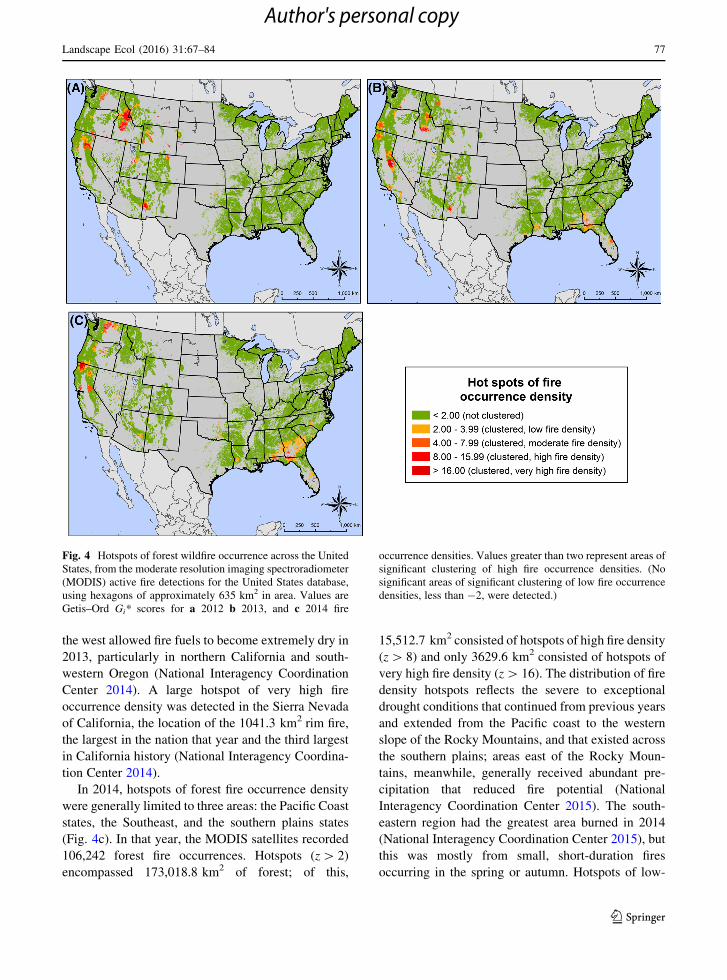
the west allowed fire fuels to become extremely dry in
2013, particularly in northern California and south-
western Oregon (National Interagency Coordination
Center 2014). A large hotspot of very high fire
occurrence density was detected in the Sierra Nevada
of California, the location of the 1041.3 km2 rim fire,
the largest in the nation that year and the third largest
in California history (National Interagency Coordina-
tion Center 2014).
In 2014, hotspots of forest fire occurrence density
were generally limited to three areas: the Pacific Coast
states, the Southeast, and the southern plains states
(Fig. 4c). In that year, the MODIS satellites recorded
106,242 forest fire occurrences. Hotspots (z[ 2)
encompassed 173,018.8 km2 of forest; of this,
15,512.7 km2 consisted of hotspots of high fire density
(z[ 8) and only 3629.6 km2 consisted of hotspots of
very high fire density (z[ 16). The distribution of fire
density hotspots reflects the severe to exceptional
drought conditions that continued from previous years
and extended from the Pacific coast to the western
slope of the Rocky Mountains, and that existed across
the southern plains; areas east of the Rocky Moun-
tains, meanwhile, generally received abundant pre-
cipitation that reduced fire potential (National
Interagency Coordination Center 2015). The south-
eastern region had the greatest area burned in 2014
(National Interagency Coordination Center 2015), but
this was mostly from small, short-duration fires
occurring in the spring or autumn. Hotspots of low-
Fig. 4 Hotspots of forest wildfire occurrence across the United
States, from the moderate resolution imaging spectroradiometer
(MODIS) active fire detections for the United States database,
using hexagons of approximately 635 km2 in area. Values are
Getis–Ord Gi* scores for a 2012 b 2013, and c 2014 fire
occurrence densities. Values greater than two represent areas of
significant clustering of high fire occurrence densities. (No
significant areas of significant clustering of low fire occurrence
densities, less than -2, were detected.)
Landscape Ecol (2016) 31:67–84 77
123
Author's personal copy

(z[ 2) to moderate (z[ 4) fire occurrence density
were detected in southwestern Georgia, the western
panhandle of Florida, and southern peninsular Florida
(Fig. 4c).
Discussion
Broad-scale ecological monitoring efforts fall within
the realm of macrosystems ecology because they
occur at regional to continental extents while incor-
porating biological, geophysical and social compo-
nents occurring at smaller scales (Heffernan et al.
2014). As such, they present the ‘‘big data’’ challenges
of macrosystems ecology, including data collection
and management, analytical complexity, and appro-
priate handling of scale issues (Heffernan et al. 2014;
Levy et al. 2014; Ruegg et al. 2014). Broad-scale
ecological monitoring requires flexible approaches
that are quantitative, scalable, and applicable to many
types of data, while allowing for the rigorous testing of
hypotheses within a spatial framework. The spatial
association of scalable hexagons (SASH) method
described here consists of three steps (1) division of
the analysis extent into equal-area hexagons of the
appropriate size (scaling), (2) aggregation of the data
within these hexagons, and (3) completion of a Getis–
Ord hotspot analysis (Getis and Ord 1992) to identify
statistically significant geographic clusters of
hexagons.
Scaling and aggregation
The equal-area sampling frame that underpins the
SASH approach is optimized for spatial neighborhood
analysis, and can be adjusted to the appropriate spatial
resolution based on sampling considerations, ecolog-
ical processes, or the spatial structure of the data.
Specifically, a hexagonal lattice is highly useful and
convenient for spatial neighborhood analysis because
the hexagons are compactly shaped (nearly circular),
maintain equal areas across a study region, are
independent of geopolitical boundaries, and are uni-
form in their distance to the centroids of their
neighboring hexagons. The selection of the appropri-
ate size for the hexagons is a critically important step,
given that the existence of scale-dependent spatial
variation can make re-scaling and data integration
problematic (Atkinson and Tate 2000). While there is
no consistent approach for determining proper hexa-
gon size, a reasonable guideline is to base it on the
properties of the phenomenon of interest, whether
related to ecological processes, sampling size, or
spatial dependence in the data. In general, the goal is to
minimize within-zone variability while selecting
zones that are as small as possible yet encompass
enough information for robust statistics; this can be a
challenging task, however, and sometimes may need
to rely on heuristics (sensu Wong 2009). We recom-
mended three possible approaches for selecting
hexagon size, and applied each in a separate analysis,
choosing a size at which hexagons (1) are as small as
possible while encompassing enough data to allow for
robust statistical analysis, (2) reflect the scale over
which an ecological phenomenon occurs or over
which management and monitoring priorities can be
decided, or (3) encompass the distance at which spatial
autocorrelation is maximized across the sample data
set. When in doubt about appropriate hexagon size,
researchers also can vary sizes based on reasonable
estimates (such as those defined by expert knowledge)
to ensure the robustness of spatial patterns across a
sensible range.
While data aggregation will cause some loss of
information, it is a necessary step to generate meaning-
ful results when assessing fine-scale data collected
across a broad area. Selecting the appropriate hexagon
size should help minimize the loss of important
information. Depending on the type of data analyzed,
it may be necessary to standardize data within hexagons
to avoid biasing the results; not standardizing data based
on the amount of forest, for example, could miss large
proportional problems in areas with small amounts of
forest or mistakenly identify small proportional prob-
lems as large problems in areas with much forest. We
standardized both the MODIS satellite fire detection
data and the mountain pine beetle aerial survey
detection data. Similarly, the aggregation of data
collected across time requires careful consideration,
and may depend on management needs, on environ-
mental patterns and processes, or on data collection
considerations. For example, although beyond the scope
of this paper, analyses of invasive species metrics
during different five-year FIA measurement cycles
could offer a sense of areas where nonnative species
have recently become more problematic. We were able
to detect such temporal patterns in mortality caused by
MPB within three four-year periods.
78 Landscape Ecol (2016) 31:67–84
123
Author's personal copy

Geographic clustering approaches
Multiple geographic clustering approaches are used in
ecology (Coulston and Riitters 2003; Hernandez-
Manrique et al. 2012; Bone et al. 2013; Timilsina
et al. 2013). All have advantages and disadvantages,
and most could be applied as cluster-detection tools
within the SASH framework. We used the Getis–Ord
Gi*statistic (Getis and Ord 1992) for the SASH
analyses presented here because, as a local indicator
of spatial association (LISA) (Anselin 1995), it is
generated by a relatively robust approach that is fairly
easy to use and allows users to test for a given level of
statistical significance while identifying hotspots and
coldspots (Nelson and Boots 2008; Johnston and
Ramachandran 2014). It also is integrated into
geographic information system packages like ArcMap
(ESRI 2012) and assigns a value to all hexagons in the
domain of analysis. Local Moran’s Ii, a different LISA
approach (Anselin 1995), has similar advantages to
Gi* while additionally offering the ability to identify
statistically significant outliers, e.g., high values
surrounded by low values. This feature was not needed
for our analyses, however. Positive values of local
Moran’s Ii indicate spatial autocorrelation in values
that are extremely positive relative to the mean, while
negative values indicate spatial autocorrelation in
values extremely negative relative to the mean; at the
same time, it is impossible to tell whether values near
zero have no spatial autocorrelation or have autocor-
relation in values close to the mean (Nelson and Boots
2008), which is a potential disadvantage.
One caveat for both LISAs is that testing for local
measures of spatial autocorrelation can be affected
by the potential presence of global spatial autocor-
relation (i.e., across the analysis extent) or by the
statistical problems associated with conducting mul-
tiple comparisons (Nelson and Boots 2008; Johnston
and Ramachandran 2014). Both Gi* and local
Moran’s Ii are relatively robust to the size of the
local neighborhood, with the same general areas of
significance detected regardless of how the local
neighborhood is defined, although larger spatial
neighborhoods tend to result in a greater number of
hotspots (Nelson and Boots 2008). Meanwhile, it is
important to note that the regional extent of an
analysis can strongly affect LISAs. The selection of
the appropriate regional extent is therefore critical,
and should be based on data considerations (e.g., the
FIA program’s use of a consistent list of problematic
invasive species across the southern United States),
the extent of the phenomenon (e.g., MPB occurring
only in the western United States), or the extent at
which regional policy and/or management decisions
are made (e.g., fire occurrence densities across the
entire United States).
Another family of cluster detection methods scan a
study area to find subregions with atypical values
(Rogerson 2010). One of the most widely used,
especially in epidemiological studies, applies a like-
lihood ratio test to examine spatial and/or temporal
windows of different size and length to assess the
randomness of phenomena (e.g., Kulldorff and Nagar-
walla 1995; Kulldorff et al. 2009). This approach,
which also has been used in forest health monitoring
applications, is able to detect geographic clusters with
significantly high rates of a phenomenon and to rank
the clusters according to the statistical likelihood that
the observed rate is higher than the background rate; it
does so regardless of the actual spatial pattern of the
clusters and without having to specify cluster sizes and
regions in advance (Coulston and Riitters 2003;
Riitters and Coulston 2005). At the same time, users
must choose from among many scan statistic param-
eters and probabilistic models based on the needs of a
given application (Costa and Kulldorff 2009), which
requires a thorough understanding of the relatively
complicated approach. Additionally, computationally
intensive spatial scan tools do not currently incorpo-
rate strong cartographic capabilities, and therefore are
inefficient for making easily interpretable maps.
Kernel estimation is a third approach for identifying
spatial variability in a phenomenon of interest, by
portraying local values that are weighted by the values
of other observations in a neighborhood, with closer
locations having greater weights (Rogerson 2001;
Nelson and Boots 2008). Kernel-estimated surfaces
can easily depict locations of abundance and scarcity
of a phenomenon, as well as spatial variability (Nelson
et al. 2006). Although a useful data exploration
technique, kernel estimation is not able to determine
the statistical significance of locations with higher or
lower values (Rogerson 2001), and is only applicable
to point data. Additionally, the amount of smoothing
used in kernel estimation, which is determined by the
neighborhood from which values are averaged, has a
large impact on kernel results (Kelsall and Diggle
1995). Small neighborhoods will reveal small-scale
Landscape Ecol (2016) 31:67–84 79
123
Author's personal copy

features of the data, while larger neighborhoods will
reveal more general features, requiring a degree of
subjectivity in choosing an appropriate neighborhood
size (Nelson and Boots 2008).
Example analyses
The flexibility of the SASH approach is demonstrated
by three examples, which encompassed a variety of
data types, spatial extents, hexagon sizes, and data
collection timeframes. Furthermore, each of these
analyses highlighted a different aspect of forest health,
illustrating the utility of the SASH approach across a
wide range of ecological phenomena.
Nonnative invasive plant species
Invasions by nonnative plant species may cause severe
and long-term impacts on forested ecosystems (Martin
et al. 2009) and ecosystem services (Pejchar and
Mooney 2009). Because nonnative species continue to
be introduced via trade and transportation, and
because their impacts will likely increase with ongo-
ing expansion of global commerce (Lodge et al. 2006;
Hulme 2009), it is critically important to synthesize
existing data on nonnative species abundance and
distributions (Crall et al. 2006) and to be able to
understand the spatial context of these data (as
illustrated here) in order to detect regions of particular
concern. Using the SASH approach, we located
geographic hotspots and coldspots of nonnative inva-
sive plant species diversity and cover across the
southeastern United States. The analysis illustrates a
way to identify locations where nonnative invasive
plant species are concentrated and where they poten-
tially have the greatest ecological impact, i.e., where
invasive cover is greatest (Hillebrand et al. 2008).
Such information may be useful in understanding
macroscale invasion patterns and for targeting activ-
ities to detect and control nonnative invasive plant
species. The SASH approach may also represent a new
cost-effective diagnostic technology that can be used
to increase active surveillance and sharing of infor-
mation about invasive species so responses to new
invasions can be more rapid and effective (Lodge et al.
2006). Datasets, such as in the FIA plot system, that
are collected consistently and in a standardized
fashion at relatively high density across broad scales
may not be available in other parts of the world, but
similar analyses are possible at a coarser scale (i.e.,
using larger hexagons) for other data sources.
Mountain pine beetle
Diseases and insects cause changes in forest structure
and function, species succession, and biodiversity, all
of which may be considered negative or positive
depending on management objectives (Edmonds et al.
2011). Analyzing patterns of forest insect infestations,
disease occurrences, forest declines and related biotic
stress factors is necessary to monitor the health of
forested ecosystems and for understanding the poten-
tial impacts of these stressors on forest structure,
composition, biodiversity, and species distributions
(Castello et al. 1995). Using the SASH approach, we
analyzed exposure to forest mortality associated with
the MPB epidemic across the western United States
during three four-year analysis windows. Such large-
scale assessments offer a useful approach for identi-
fying geographic areas where the concentration of
management activities might be most effective (e.g.,
Potter and Paschke 2015) or where risk of future
outbreaks is highest (e.g., Bone et al. 2013). Further-
more, the SASH approach provides a straightforward
framework for continued monitoring of outbreaks,
which is necessary for determining appropriate fol-
low-up investigations. Specific examples with respect
to MPB include efforts to understand the interaction
between beetle-associated mortality and other forest
disturbances such as climate change, wildland fire, and
harvest; to quantify impacts to timber, wildlife,
recreation, and water; and to construct ecosystem
models that evaluate impacts on biochemical and
biophysical processes (Meddens et al. 2012).
Fire occurrence
As a key agent of disturbance operating at many
spatial and temporal scales, wildland fire affects forest
health both positively and negatively (Edmonds et al.
2011; Lundquist et al. 2011). Ecological and forest
health impacts relating to fire and other abiotic
disturbances are scale-dependent properties which in
turn are affected by management objectives (Lund-
quist et al. 2011). Quantifying and monitoring large-
scale patterns of fire occurrence also may help
improve understanding of the ecological and eco-
nomic impacts of fire, as well as the appropriate
80 Landscape Ecol (2016) 31:67–84
123
Author's personal copy

management and prescribed use of fire. Specifically,
spatially explicit assessments of fire occurrence could
help identify relatively compact areas where specific
management activities may be necessary, or where
research into the ecological and socioeconomic
impacts of fires may be required (e.g., Tonini et al.
2009; Potter 2015b). Using the SASH approach, we
present analyses of high-temporal-fidelity fire occur-
rence data, collected by satellite, that map where fire
occurrences have been concentrated spatially across
the conterminous United States during three recent
years. Similar analyses are possible in other areas of
the world, such as Australia (Oliveira et al. 2015),
Latin America (Portillo-Quintero et al. 2013), Russia
(Krylov et al. 2014), and India (Vadrevu et al. 2008),
where MODIS and other satellite data have been
applied in broad-scale analyses of fire detections.
Conclusions
Fine-scale ecological data are becoming increasingly
available across broad regions. Presenting this infor-
mation in ways that are relevant for policy and
management decisions is critically important (e.g.,
Hooper et al. 2005), but poses a major challenge.
Specifically, doing so requires a framework that
aggregates information to a spatial scale at which
ecological processes occur or at which decisions can
be made, and that can help to discern which areas need
the most attention. We propose a flexible approach
that identifies statistically significant geographic clus-
ters of ecological phenomena after aggregating fine-
scale data into scalable hexagonal cells across broad
extents. The SASH method described here is based on
an equal-area sampling frame that is optimized for
spatial neighborhood analysis and that can be adjusted
to the appropriate spatial resolution.
Because creative geographic analyses of broad-
scale data are necessary to identify places where
indicators suggest the existence of relatively poor
forest health conditions (Coulston and Riitters 2003),
the SASH analytical approach has become a founda-
tional element of annual USDA Forest Service
national reports on the status and trends of forest
health across the nation (e.g., Potter 2015b; Potter and
Paschke 2015). The results of these analyses are used
by researchers and managers to select finer-scale
locations for follow-up research activities. For the
analyses described here and in the Forest Service
reports, it is fortuitous that the United States is data-
rich, with the existence of several fine-scale standard-
ized ecological datasets that span the extent of the
country. The SASH method is not limited to North
America, however, and is a ‘‘big data’’ analysis tool
that, regardless of region, has potential application for
a broad range of macrosystems ecology studies
requiring the rigorous testing of hypotheses within a
spatial framework. The North American hexagon that
was the foundation of the analyses presented here is, in
fact, a single face of a truncated icosahedron fit to the
globe (White et al. 1992). That global truncated
icosahedron can be configured to position a hexagon
over any area of interest, which can then be subdivided
into multiple hexagons of appropriate area. Tools also
can be imported into Geographic Information Systems
programs to generate hexagons of desired size for a
given study region. Additionally, while it is desirable
to use fine-scale data collected in a standardized
fashion and at a high sampling intensity, the lack of
such data is not necessarily a limitation. In such cases,
the flexibility of the SASH method allows for the
aggregation of data to larger hexagons and, therefore,
to coarser scales of analysis.
Acknowledgments The authors thank Stan Zarnoch, Kurt
Riitters, John Coulston, and Joe Spruce for their advice and
assistance; Jeanine Paschke for her help with the aerial survey
data; and two anonymous reviewers for their helpful comments.
The authors also thank the Forest Inventory and Analysis field
crew members and the forest health aerial survey detection
teams for their efforts to collect the data used in this study. This
research was supported in part through Cost Share Agreement
14-CS-11330110-042 between the USDA Forest Service and
North Carolina State University, and through a National Science
Foundation MacroSystems Biology Grant (#1241932).
References
Anselin L (1992) Spatial data analysis with GIS: an introduction
to application in the social sciences. National Center for
Geographic Information and Analysis, Santa Barbara
Anselin L (1995) Local indicators of spatial association—LISA.
Geogr Anal 27(2):93–115
Atkinson PM, Tate NJ (2000) Spatial scale problems and geo-
statistical solutions: a review. Prof Geogr 52(4):607–623.
doi:10.1111/0033-0124.00250
Bechtold WA, Patterson PL (2005) The enhanced forest
inventory and analysis program: national sampling design
and estimation procedures. USDA Forest Service, South-
ern Research Station, Asheville
Landscape Ecol (2016) 31:67–84 81
123
Author's personal copy

Bechtold WA, Scott CT (2005) The forest inventory and anal-
ysis plot design. In: Bechtold WA, Patterson PL (eds) The
enhanced forest inventory and analysis program—national
sampling design and estimation procedures., General
Technical Report SRS-80United States Department of
Agriculture, Forest Service, Southern Research Station,
Asheville, pp 27–42
Bone C,Wulder MA,White JC, Robertson C, Nelson TA (2013)
A GIS-based risk rating of forest insect outbreaks using
aerial overview surveys and the local Moran’s I statistic.
Appl Geogr 40:161–170. doi:10.1016/j.apgeog.2013.02.
011
Castello JD, Leopold DJ, Smallidge PJ (1995) Pathogens, pat-
terns, and processes in forest ecosystems. Bioscience
45(1):16–24
Cliff AD, Ord JK (1981) Spatial processes: models and appli-
cations. Pion, London
Costa MA, Kulldorff M (2009) Applications of spatial scan
statistics: a review. Scan Statistics: methods and applica-
tions. Birkhauser, Boston. doi:10.1007/978-0-8176-4749-
0_6
Coulston JW, Riitters KH (2003) Geographic analysis of forest
health indicators using spatial scan statistics. Environ
Manage 31(6):764–773
Crall AW, Meyerson LA, Stohlgren TJ, Jarnevich CS, Newman
GJ, Graham J (2006) Show me the numbers: what data
currently exist for non-native species in the USA? Front
Ecol Environ 4(8):414–418
Dark SJ, Bram D (2007) The modifiable areal unit problem
(MAUP) in physical geography. Prog Phys Geogr
31(5):471–479. doi:10.1177/0309133307083294
Edmonds RL, Agee JK, Gara RI (2011) Forest health and pro-
tection, 2nd edn. Waveland Press Inc., Long Grove
ESRI (2012) ArcMap 10.1. Environmental Systems Research
Institute Inc., Redlands
Fotheringham AS,Wong DWS (1991) The modifiable areal unit
problem in multivariate statistical analysis. Environ Plan A
23(7):1025–1044. doi:10.1068/a231025
Getis A, Ord JK (1992) The analysis of spatial association by use
of distance statistics. Geogr Anal 24(3):189–206
Hawbaker TJ, Radeloff VC, Syphard AD, Zhu ZL, Stewart SI
(2008) Detection rates of the MODIS active fire product in
the United States. Remote Sens Environ 112(5):2656–
2664. doi:10.1016/j.rse.2007.12.008
Heffernan JB, Soranno PA, Angilletta MJ, Buckley LB, Gruner
DS, Keitt TH, Kellner JR, Kominoski JS, Rocha AV, Xiao
JF, Harms TK, Goring SJ, Koenig LE, McDowell WH,
Powell H, Richardson AD, Stow CA, Vargas R, Weathers
KC (2014) Macrosystems ecology: understanding ecolog-
ical patterns and processes at continental scales. Front Ecol
Environ 12(1):5–14. doi:10.1890/130017
Hernandez-Manrique OL, Sanchez-Fernandez D, Verdu JR,
Numa C, Galante E, Lobo JM (2012) Using local auto-
correlation analysis to identify conservation areas: an
example considering threatened invertebrate species in
Spain. Biodivers Conserv 21(8):2127–2137. doi:10.1007/
s10531-012-0303-5
Hillebrand H, Bennett DM, Cadotte MW (2008) Consequences
of dominance: a review of evenness effects on local and
regional ecosystem processes. Ecology 89(6):1510–1520.
doi:10.1890/07-1053.1
Hong SY, O’Sullivan D (2012) Detecting ethnic residential
clusters using an optimisation clustering method. Int J
Geogr Inf Sci 26(8):1457–1477. doi:10.1080/13658816.
2011.637045
Hooper DU, Chapin FS, Ewel JJ, Hector A, Inchausti P, Lavorel
S, Lawton JH, Lodge DM, Loreau M, Naeem S, Schmid B,
Setala H, Symstad AJ, Vandermeer J, Wardle DA (2005)
Effects of biodiversity on ecosystem functioning: a con-
sensus of current knowledge. Ecol Monogr 75(1):3–35
Hulme PE (2009) Trade, transport and trouble: managing
invasive species pathways in an era of globalization. J Appl
Ecol 46(1):10–18. doi:10.1111/j.1365-2664.2008.01600.x
Iannone BV, Oswalt CM, Liebhold AM, Guo Q, Potter KM,
Nunez-Mir GC, Oswalt SN, Pijanowski BC, Fei S (2015)
Region-specific patterns and drivers of macroscale forest
plant invasions. Divers Distrib 21:1181–1192
Jelinski DE, Wu JG (1996) The modifiable areal unit problem
and implications for landscape ecology. Landscape Ecol
11(3):129–140. doi:10.1007/bf02447512
Johnston RJ, Ramachandran M (2014) Modeling spatial patch-
iness and hot spots in stated preference willingness to pay.
Environ Resour Econ 59(3):363–387. doi:10.1007/s10640-
013-9731-2
Justice CO, Giglio L, Korontzi S, Owens J, Morisette JT, Roy D,
Descloitres J, Alleaume S, Petitcolin F, Kaufman Y (2002)
The MODIS fire products. Remote Sens Environ
83(1–2):244–262. doi:10.1016/s0034-4257(02)00076-7
Justice CO, Giglio L, Roy D, Boschetti L, Csiszar I, Davies D,
Korontzi S, Schroeder W, O’Neal K, Morisette J (2011)
MODIS-derived global fire products. In: Ramachandran B,
Justice CO, Abrams MJ (eds) Land remote sensing and
global environmental change: NASA’s earth observing
system and the science of ASTER and MODIS. Springer,
New York, pp 661–679
Kamei M, Nakagoshi N (2006) Geographic assessment of pre-
sent protected areas in Japan for representativeness of
forest communities. Biodivers Conserv 15(14):4583–4600.
doi:10.1007/s10531-005-5822-x
Kelsall JE, Diggle PJ (1995) Non-parametric estimation of
spatial variation in relative risk. Stat Med
14(21–22):2335–2342. doi:10.1002/sim.4780142106
Krylov A, McCarty JL, Potapov P, Loboda T, Tyukavina A,
Turubanova S, HansenMC (2014) Remote sensing estimates
of stand-replacement fires in Russia, 2002–2011. Environ
Res Lett 9(10):8. doi:10.1088/1748-9326/9/10/105007
Kulldorff M, Nagarwalla N (1995) Spatial disease clusters:
detection and inference. Stat Med 14(8):799–810. doi:10.
1002/sim.4780140809
Kulldorff M, Huang L, Konty K (2009) A scan statistic forcontinuous data based on the normal probability model. Int
J Health Geogr 8:9. doi:10.1186/1476-072x-8-58
Kwan MP (2012) The uncertain geographic context problem.
Ann Assoc Am Geogr 102(5):958–968. doi:10.1080/
00045608.2012.687349
Laffan SW (2006) Assessing regional scale weed distributions,
with an Australian example using Nassella trichotoma.
Weed Res 46(3):194–206
Lepczyk CA, Hammer RB, Stewart SI, Radeloff VC (2007)
Spatiotemporal dynamics of housing growth hotspots in the
North Central U.S. from, 1940 to 2000. Landscape Ecol
22(6):939–952
82 Landscape Ecol (2016) 31:67–84
123
Author's personal copy

Levy O, Ball BA, Bond-Lamberty B, Cheruvelil KS, Finley AO,
Lottig NR, Punyasena SW, Xiao JF, Zhou JZ, Buckley LB,
Filstrup CT, Keitt TH, Kellner JR, Knapp AK, Richardson
AD, Tcheng D, Toomey M, Vargas R, Voordeckers JW,
Wagner T, Williams JW (2014) Approaches to advance
scientific understanding of macrosystems ecology. Front
Ecol Environ 12(1):15–23. doi:10.1890/130019
Lodge DM, Williams S, MacIsaac HJ, Hayes KR, Leung B,
Reichard S, Mack RN, Moyle PB, Smith M, Andow DA,
Carlton JT, McMichael A (2006) Biological invasions:
recommendations for US policy and management. Ecol
Appl 16(6):2035–2054. doi:10.1890/1051-0761(2006)016
[2035:birfup]2.0.co;2
Lundquist JE, Camp AE, Tyrrell ML, Seybold SJ, Cannon P,
Lodge DJ (2011) Earth, wind and fire: abiotic factors and
the impacts of global environmental change on forest
health. In: Castello JD, Teale SA (eds) Forest health: an
integrated perspective. Cambridge University Press, New
York, pp 195–243
Ma ZH, Zuckerberg B, Porter WF, Zhang LJ (2012) Use of
localized descriptive statistics for exploring the spatial
pattern changes of bird species richness at multiple scales.
Appl Geogr 32(2):185–194. doi:10.1016/j.apgeog.2011.
05.005
Martin PH, Canham CD, Marks PL (2009) Why forests appear
resistant to exotic plant invasions: intentional introduc-
tions, stand dynamics, and the role of shade tolerance.
Front Ecol Environ 7(3):142–149. doi:10.1890/070096
Meddens AJH, Hicke JA, Ferguson CA (2012) Spatiotemporal
patterns of observed bark beetle-caused tree mortality in
British Columbia and the western United States. Ecol Appl
22(7):1876–1891
National Interagency Coordination Center (2013) Wildland fire
summary and statistics annual report: 2012. http://www.
predictiveservices.nifc.gov/intelligence/2012_statssumm/
intro_summary.pdf. Accessed 14 May 2013
National Interagency Coordination Center (2014) Wildland fire
summary and statistics annual report: 2013. http://www.
predictiveservices.nifc.gov/intelligence/2013_Statssumm/
intro_summary13.pdf. Accessed 28 May 2014
National Interagency Coordination Center (2015) Wildland fire
summary and statistics annual report: 2014. http://www.
predictiveservices.nifc.gov/intelligence/2014_Statssumm/
intro_summary14.pdf. Accessed 11 May 2015
Nelson TA, Boots B (2008) Detecting spatial hot spots in
landscape ecology. Ecography 31(5):556–566. doi:10.
1111/j.0906-7590.2008.05548.x
Nelson T, Boots B, Wulder MA (2006) Large-area mountain
pine beetle infestations: spatial data representation and
accuracy. For Chron 82(2):243–252
Netto SMB, Silva AC, Nunes RA, Gattass M (2012) Analysis of
directional patterns of lung nodules in computerized
tomography using Getis statistics and their accumulated
forms as malignancy and benignity indicators. Pattern
Recognit Lett 33(13):1734–1740. doi:10.1016/j.patrec.
2012.05.010
Oliver MA (2001) Determining the spatial scale of variation in
environmental properties using the variogram. In: Tate NJ,
Atkinson PM (eds) Modelling scale in geographical
information science. Wiley, Chicester, pp 193–219
Oliveira SLJ, Maier SW, Pereira JMC, Russell-Smith J (2015)
Seasonal differences in fire activity and intensity in tropical
savannas of northern Australia using satellite measure-
ments of fire radiative power. Int J Wildland Fire
24(2):249–260. doi:10.1071/wf13201
Openshaw S (1977) Geographical solution to scale and aggre-
gation problems in region-building, partitioning and spatial
modeling. Trans Inst Br Geogr 2(4):459–472. doi:10.2307/
622300
Ord JK, Getis A (1995) Local spatial autocorrelation statistics:
distributional issues and an application. Geogr Anal
27(4):286–306
Oswalt CM, Fei S, Guo Q, Iannone BV, Oswalt S, Pijanowski B,
Potter KM (2015) A subcontinental view of forest plant
invasions using national inventory data. Neobiota
24:49–54
Palmer MW (2002) Scale detection using semivariograms and
autocorrelograms. In: Gergel SE, Turner MG (eds)
Learning landscape ecology: a practical guide to concepts
and techniques. Springer, New York, pp 129–144
Pejchar L, Mooney HA (2009) Invasive species, ecosystem
services and human well-being. Trends Ecol Evol
24(9):497–504. doi:10.1016/j.tree.2009.03.016
Portillo-Quintero C, Sanchez-Azofeifa A, do Espirito-Santo
MM (2013) Monitoring deforestation with MODIS active
fires in neotropical dry forests: an analysis of local-scale
assessments in Mexico, Brazil and Bolivia. J Arid Environ
97:150–159. doi:10.1016/j.jaridenv.2013.06.002
Potter KM (2015a) Large-scale patterns of forest fire occurrence
in the conterminous United States and Alaska, 2012. In:
Potter KM, Conkling BL (eds) Forest health monitoring:
national status, trends and analysis, 2013, vol general
technical report SRS-207. U.S. Department of Agriculture,
Forest Service, Southern Research Station, Asheville,
pp 37–53
Potter KM (2015b) Large-scale patterns of forest fire occurrence
in the conterminous United States and Alaska 2013. In:
Potter KM, Conkling BL (eds) Forest health monitoring:
national status, trends and analysis, 2014, vol general
technical report SRS-209. U.S. Department of Agriculture,
Forest Service, Southern Research Station, Asheville,
pp 39–55
Potter KM, Koch FH (2014) Phylogenetic community structure
of forests across the conterminous United States: regional
ecological patterns and forest health implications. For Sci
60(2):851–861. doi:10.5849/forsci.13-115
Potter KM, Paschke JL (2015) Large-scale patterns of insect and
disease activity in the conterminous United States, Alaska,
and Hawaii from the national insect and disease survey
2013. In: Potter KM, Conkling BL (eds) Forest health
monitoring: national status, trends and analysis, 2014, vol
general technical report SRS-209. U.S. Department of
Agriculture, Forest Service, Southern Research Station,
Asheville, pp 19–38
Potter KM, Woodall CW (2012) Trends over time in tree and
seedling phylogenetic diversity indicate regional differ-
ences in forest biodiversity change. Ecol Appl 22(2):517–
531
Prestemon JP, Abt KL, Potter KM, Koch FH (2013) An eco-
nomic assessment of mountain pine beetle timber salvage
Landscape Ecol (2016) 31:67–84 83
123
Author's personal copy

in the west. West J Appl For 28(4):143–153. doi:10.5849/
wjaf.12-032
Raffa KF, Aukema BH, Bentz BJ, Carroll AL, Hicke JA, Turner
MG, Romme WH (2008) Cross-scale drivers of natural
disturbances prone to anthropogenic amplification: the
dynamics of bark beetle eruptions. Bioscience 58(6):
501–517. doi:10.1641/b580607
Reams GA, SmithWD, Hansen MH, Bechtold WA, Roesch FA,
Moisen GG (2005) The forest inventory and analsysis
sampling frame. In: Bechtold WA, Patterson PL (eds) The
enhanced forest inventory and analysis program—national
sampling design and estimation procedures., General
Technical Report SRS-80United States Department of
Agriculture, Forest Service, Southern Research Station,
Asheville, pp 11–26
Ries P, Dix ME, Lelmini M, Thomas D (2004) National strategy
and implementation plan for invasive species management.
United States Department of Agriculture, Forest Service,
Washington, DC
Riitters KH, Coulston JW (2005) Hot spots of perforated forest
in the eastern United States. Environ Manag 35(4):
483–492. doi:10.1007/s00267-003-0220-1
Riitters KH, Tkacz B (2004) The U.S. forest health monitoring
program. In: Wiersma GB (ed) Environmental monitoring.
CRC Press, Boca Raton, pp 669–683
Riitters KH, Wickham JD (2012) Decline of forest interior
conditions in the conterminous United States. Sci Rep 2:4.
doi:10.1038/srep00653
RockyMountain Region Forest Health Protection (2010) A field
guide to insects and diseases of the Rocky Mountain
region. U. S. Department of Agriculture Forest Service.
Rocky Mountain Research Station, Fort Collins
Rogerson PA (2001) A statistical method for the detection of
geographic clustering. Geogr Anal 33(3):215–227
Rogerson PA (2010) Optimal geographic scales for local spatial
statistics. Stat Methods Med Res 20(2):119–129. doi:10.
1177/0962280210369039
Ruegg J, Gries C, Bond-Lamberty B, Bowen GJ, Felzer BS,
McIntyre NE, Soranno PA, Vanderbilt KL, Weathers KC
(2014) Completing the data life cycle: using information
management in macrosystems ecology research. Front
Ecol Environ 12(1):24–30. doi:10.1890/120375
Schulz BK, Gray AN (2013) The new flora of northeastern USA:
quantifying introduced plant species occupancy in forest
ecosystems. Environ Monit Assess 185(5):3931–3957.
doi:10.1007/s10661-012-2841-4
Shima T, Sugimoto S, Okutomi M (2010) Comparison of image
alignment on hexagonal and square lattices. In: 2010 IEEE
international conference on image processing, pp 141–144.
doi:10.1109/icip.2010.5654351
Shore TL, Safranyik L (1992) Susceptibility and risk rating
systems for the mountain pine beetle in lodgepole pine
stands. Forestry Canada, Pacific Forestry Centre, Victoria
Smith WB (2002) Forest inventory and analysis: a national
inventory and monitoring program. Environ Pollut
116:S233–S242
Smith WB, Miles PD, Perry CH, Pugh SA (2009) Forest
resources of the United States, 2007. U.S. Department of
Agriculture Forest Service, Washington Office, Washing-
ton, DC
Sokal RR, Oden NL, Thomson BA (1998) Local spatial auto-
correlation in a biological model. Geogr Anal 30(4):
331–354
Timilsina N, Escobedo FJ, Cropper WP, Abd-Elrahman A,
Brandeis TJ, Delphin S, Lambert S (2013) A framework for
identifying carbon hotspots and forest management drivers.
J Environ Manag 114:293–302. doi:10.1016/j.jenvman.
2012.10.020
Tonini M, Tuia D, Ratle F (2009) Detection of clusters using
space-time scan statistics. Int J Wildland Fire 18(7):
830–836. doi:10.1071/wf07167
United States Department of Agriculture Forest Service (2008)
National forest type data development. United States
Department of Agriculture, Forest Service, Forest Inven-
tory and Analysis, Remote Sensing Applications Center.
http://svinetfc4.fs.fed.us/rastergateway/forest_type/. Accessed 13
May 2008
United States Department of Agriculture Forest Service (2011)
National report on sustainable forests—2010. U.S.
Department of Agriculture Forest Service, Washington,
DC
United States Department of Agriculture Forest Service (2015a)
Insect and disease detection survey database (IDS). Digital
data. U.S. Department of Agriculture Forest Service, Forest
Health Protection, Forest Health Technology Enterprise
Team. http://foresthealth.fs.usda.gov/ids. Accessed 13
April 2015
United States Department of Agriculture Forest Service (2015b)
MODIS active fire mapping program: continental United
States fire detection GIS data. U.S. Department of Agri-
culture, Forest Service, Remote Sensing Application
Center. http://activefiremaps.fs.fed.us/gisdata.php. Acces-
sed 13 Feb 2015
Vadrevu KP, Badarinath KVS, Eaturu A (2008) Spatio-temporal
analysis of fire events in India: implications for environ-
mental conservation. J Environ Plan Manag 51(6):
817–832. doi:10.1080/09640560802423657
Waller LA, Gotway CA (2004) Applied spatial statistics for
public health data. Wiley, Hoboken
White D, Kimerling AJ, Overton WS (1992) Cartographic and
geometric components of a global sampling design for
environmental monitoring. Cartogr Geogr Inf Syst 19(1):
5–22
Wong D (2009) The modifiable areal unit problem (MAUP). In:
Fotheringham AS, Rogerson PA (eds) The SAGE hand-
book of spatial analysis. SAGE Publications Ltd., London,
pp 105–125
Woudenberg SW, Conkling BL, O’Connell BM, LaPoint EB,
Turner JA, Waddell KL (2010) The forest inventory and
analysis database: database description and users manual
version 4.0 for phase 2. USDA Forest Service, Rocky
Mountain Research Station, Fort Collins
84 Landscape Ecol (2016) 31:67–84
123
Author's personal copy