data gathering and personalized broadcasting in radio
TRANSCRIPT

HAL Id: hal-01084996https://hal.inria.fr/hal-01084996
Submitted on 20 Nov 2014
HAL is a multi-disciplinary open accessarchive for the deposit and dissemination of sci-entific research documents, whether they are pub-lished or not. The documents may come fromteaching and research institutions in France orabroad, or from public or private research centers.
L’archive ouverte pluridisciplinaire HAL, estdestinée au dépôt et à la diffusion de documentsscientifiques de niveau recherche, publiés ou non,émanant des établissements d’enseignement et derecherche français ou étrangers, des laboratoirespublics ou privés.
Data gathering and personalized broadcasting in radiogrids with interference
Jean-Claude Bermond, Bi Li, Nicolas Nisse, Hervé Rivano, Min-Li Yu
To cite this version:Jean-Claude Bermond, Bi Li, Nicolas Nisse, Hervé Rivano, Min-Li Yu. Data gathering and personal-ized broadcasting in radio grids with interference. Theoretical Computer Science, Elsevier, 2015, 562,pp.453-475. �10.1016/j.tcs.2014.10.029�. �hal-01084996�
JID:TCS AID:9926 /FLA Doctopic: Algorithms, automata, complexity and games [m3G; v1.143-dev; Prn:6/11/2014; 9:19] P.1 (1-23)
Theoretical Computer Science ••• (••••) •••–•••
Contents lists available at ScienceDirect
Theoretical Computer Science
www.elsevier.com/locate/tcs
Data gathering and personalized broadcasting in radio grids
with interference ✩
Jean-Claude Bermond a,b,∗, Bi Li b,a,c, Nicolas Nisse b,a, Hervé Rivano d, Min-Li Yu e
a Univ. Nice Sophia Antipolis, CNRS, I3S, UMR 7271, Sophia Antipolis, Franceb INRIA, Francec Institute of Applied Mathematics, Chinese Academy of Sciences, Beijing, Chinad Urbanet Inria team, Université de Lyon, Insa Lyon Inria CITI Lab, Francee University of the Fraser Valley, Dpt of Maths and Statistics, Abbotsford, BC, Canada
a r t i c l e i n f o a b s t r a c t
Article history:Received 29 December 2012Received in revised form 8 October 2014Accepted 21 October 2014Available online xxxxCommunicated by G. Ausiello
Keywords:GatheringPersonalized broadcastingGridInterferenceRadio networks
In the gathering problem, a particular node in a graph, the base station, aims at receiving messages from some nodes in the graph. At each step, a node can send one message to one of its neighbors (such an action is called a call). However, a node cannot send and receive a message during the same step. Moreover, the communication is subject to interference constraints, more precisely, two calls interfere in a step, if one sender is at distance at most dI from the other receiver. Given a graph with a base station and a set of nodes having some messages, the goal of the gathering problem is to compute a schedule of calls for the base station to receive all messages as fast as possible, i.e., minimizing the number of steps (called makespan). The gathering problem is equivalent to the personalized broadcasting problem where the base station has to send messages to some nodes in the graph, with same transmission constraints.In this paper, we focus on the gathering and personalized broadcasting problem in grids. Moreover, we consider the non-buffering model: when a node receives a message at some step, it must transmit it during the next step. In this setting, though the problem of determining the complexity of computing the optimal makespan in a grid is still open, we present linear (in the number of messages) algorithms that compute schedules for gathering with dI ∈ {0, 1, 2}. In particular, we present an algorithm that achieves the optimal makespan up to an additive constant 2 when dI = 0. If no messages are “close” to the axes (the base station being the origin), our algorithms achieve the optimal makespan up to an additive constant 1 when dI = 0, 4 when dI = 2, and 3 when both dI = 1 and the base station is in a corner. Note that, the approximation algorithms that we present also provide approximation up to a ratio 2 for the gathering with buffering. All our results are proved in terms of personalized broadcasting.
© 2014 Elsevier B.V. All rights reserved.
✩ This work is partially supported by Project STREP FP7 EULER, ANR Verso project Ecoscells, ANR GRATEL and Region PACA.
* Corresponding author at: Univ. Nice Sophia Antipolis, CNRS, I3S, UMR 7271, Sophia Antipolis, France.E-mail addresses: [email protected] (J-C. Bermond), [email protected] (B. Li), [email protected] (N. Nisse), [email protected] (H. Rivano),
[email protected] (M.-L. Yu).
http://dx.doi.org/10.1016/j.tcs.2014.10.0290304-3975/© 2014 Elsevier B.V. All rights reserved.
JID:TCS AID:9926 /FLA Doctopic: Algorithms, automata, complexity and games [m3G; v1.143-dev; Prn:6/11/2014; 9:19] P.2 (1-23)
2 J-C. Bermond et al. / Theoretical Computer Science ••• (••••) •••–•••
1. Introduction
1.1. Problem, model and assumptions
In this paper, we study a problem that was motivated by designing efficient strategies to provide internet access using wireless devices [8]. Typically, several houses in a village need access to a gateway (for example a satellite antenna) to transmit and receive data over the Internet. To reduce the cost of the transceivers, multi-hop wireless relay routing is used. We formulate this problem as gathering information in a Base Station (denoted by BS) of a wireless multi-hop network when interference constraints are present. This problem is also known as data collection and is particularly important in sensor networks and access networks.
Transmission model We adopt the network model considered in [2,4,9,11,16]. The network is represented by a node-weighted symmetric digraph G = (V , E), where V is the set of nodes and E is the set of arcs. More specifically, each node in V represents a device (sensor, station, . . . ) that can transmit and receive data. There is a special node BS ∈ V called the Base Station (BS), which is the final destination of all data possessed by the various nodes of the network. Each node may have any number of pieces of information, or messages, to transmit, including none. There is an arc from u to v if u can transmit a message to v . We suppose that the digraph is symmetric; so if u can transmit a message to v , then v can also transmit a message to u. Therefore G represents the graph of possible communications. Some authors use an undirected graph (replacing the two arcs (u, v) and (v, u) by an edge {u, v}). However calls (transmissions) are directed: a call (s, r)is defined as the transmission from the node s to node r, in which s is the sender and r is the receiver and s and r are adjacent in G . The distinction of sender and receiver is important for our interference model.
Here we consider grids as they model well both access networks and also random networks [14]. The network is assumed to be synchronous and the time is slotted into steps. During each step, a transmission (or a call) between two nodes can transport at most one message. That is, a step is a unit of time during which several calls can be done as long as they do not interfere with each other. We suppose that each device is equipped with a half duplex interface: a node cannot both receive and transmit during a step. This models the near-far effect of antennas: when one is transmitting, it’s own power prevents any other signal to be properly received. Moreover, we assume that a node can transmit or receive at most one message per step.
Following [11,12,15,16,18] we assume that no buffering is done at intermediate nodes and each node forwards a message as soon as it receives it. One of the rationales behind this assumption is that it frees intermediate nodes from the need to maintain costly state information and message storage.
Interference model We use a binary asymmetric model of interference based on the distance in the communication graph. Let d(u, v) denote the distance, that is the length of a shortest directed path, from u to v in G and dI be a nonnegative integer. We assume that when a node u transmits, all nodes v such that d(u, v) ≤ dI are subject to the interference from u’s transmission. We assume that all nodes of G have the same interference range dI . Two calls (s, r) and (s′, r′) do not interfere if and only if d(s, r′) > dI and d(s′, r) > dI . Otherwise calls interfere (or there is a collision). We focus on the cases where dI ≤ 2. Note that in this paper we suppose dI ≥ 0. It implies that a node cannot receive and send simultaneously.
The binary interference model is a simplified version of the reality, where the Signal-to-Noise-and-Interference Ratio (the ratio of the received power from the source of the transmission to the sum of the thermic noise and the received powers of all other simultaneously transmitting nodes) has to be above a given threshold for a transmission to be successful. However, the values of the completion times that we obtain lead to lower bounds on the corresponding real life values. Stated differently, if the completion time is fixed, then our results lead to upper bounds on the maximum possible number of messages that can be transmitted in the network.
Gathering and personalized broadcasting Our goal is to design protocols that efficiently, i.e., quickly, gather all messages to the base station BS subject to these interference constraints. More formally, let G = (V , E) be a connected symmetric digraph, BS ∈ V and dI ≥ 0 be an integer. Each node in V \ BS is assigned a set (possibly empty) of messages that must be sent to BS. A multi-hop schedule for a message is a sequence of calls used to transmit this message to BS. As no buffering is allowed, this schedule is defined by the step of the first call and the path that the message follows in order to reach BS. The gathering problem consists in computing a multi-hop schedule for each message to arrive the BS under the constraint that during any step any two calls do not interfere within the interference range dI . The completion time or makespan of the schedule is the number of steps used for all messages to reach BS. We are interested in computing the schedule with minimum makespan.
Actually, we describe the gathering schedule by illustrating the schedule for the equivalent personalized broadcasting prob-lem since this formulation allows us to use a simpler notation and simplify the proofs. In this problem, the base station BShas initially a set of personalized messages and they must be sent to their destinations, i.e., each message has a personalized destination in V , and possibly several messages may have the same destination. The problem is to find a multi-hop sched-ule for each message to reach its corresponding destination node under the same constraints as the gathering problem. The completion time or makespan of the schedule is the number of steps used for all messages to reach their destination and the problem aims at computing a schedule with minimum makespan. For any personalized broadcasting schedule, it is always possible to build a gathering schedule with the same makespan. Hence these two problems are equivalent. Indeed,

JID:TCS AID:9926 /FLA Doctopic: Algorithms, automata, complexity and games [m3G; v1.143-dev; Prn:6/11/2014; 9:19] P.3 (1-23)
J-C. Bermond et al. / Theoretical Computer Science ••• (••••) •••–••• 3
Table 1Performances of the algorithms designed in this paper. Our algorithms deal with the gathering and personalized broadcasting problems in a grid with arbitrary base station (unless stated otherwise). In this table, +c-approximation means that our algorithm achieves an optimal makespan up to an additive constant c. Similarly, ×c-approximation means that our algorithm achieves an optimal makespan up to an multiplicative constant c.
Interference Additional hypothesis Performances
without buffering with buffering
dI = 0 +2-approximationno messages on axes +1-approximation
dI = 1 BS in a corner and no messages “close” to the axes (see Definition 2) +3-approx. ×1.5-approx.no messages at distance ≤1 from an axis ×1.5-approximation
dI = 2 no messages at distance ≤1 from an axis +4-approx. ×2-approx.
consider a personalized broadcasting schedule with makespan T . Any call (s, r) occurring at step k corresponds to a call (r, s) scheduled at step T + 1 −k in the corresponding gathering schedule. Furthermore, as the digraph is symmetric, if two calls (s, r) and (s′, r′) do not interfere, then d(s, r′) > dI and d(s′, r) > dI ; so the reverse calls do not interfere. Hence, if there is an (optimal) personalized broadcasting schedule from BS, then there exists an (optimal) solution for gathering at BS with the same makespan. The reverse also holds. Therefore, in the sequel, we consider the personalized broadcasting problem.
1.2. Related work
Gathering problems like the one that we study in this paper have received much recent attention. The papers most closely related to our results are [3,4,11,12,15,16]. The data gathering problem is first introduced in [11] under a model for sensor networks similar to the one adopted in this paper. It deals with dI = 0 and gives optimal gathering schedules for trees. Optimal algorithms for star networks are given in [16] and they provide optimal schedules which minimize both the completion time and the average delivery time for all the messages. Under the same hypothesis, an optimal algorithm for general networks is presented in [12] in the case each node has exactly one message to deliver. In [4] (resp. [3]) optimal gathering algorithms for tree networks in the same model considered in the present paper, are given when dI = 1 (resp., dI ≥ 2). In [3] it is also shown that the Gathering Problem is NP-complete if the process must be performed along the edges of a routing tree for dI ≥ 2 (otherwise the complexity is not determined). Furthermore, for dI ≥ 1 a simple (1 + 2
dI)
factor approximation algorithm is given for general networks. In slightly different settings, in particular the assumption of directional antennas, the problem has been proved NP-hard in general networks [17]. The case of open-grid where BS stands at a corner and no messages have destinations in the first row or first column, called axis in the following, is considered in [15], where a 1.5-approximation algorithm is presented.
Other related results can be found in [1,2,6,7,10] (see [9] for a survey). In these articles data buffering is allowed at intermediate nodes, achieving a smaller makespan. In [2], a 4-approximation algorithm is given for any graph. In particular the case of grids is considered in [6], but with exactly one message per node. Another related model can be found in [13], where steady-state (continuous) flow demands between each pair of nodes have to be satisfied, in particular, the authors also study the gathering in radio grid networks.
1.3. Our results
In this paper, we propose algorithms to solve the personalized broadcasting problem (and so the equivalent gathering problem) in a grid with the model described above (synchronous, no buffering, one message transmission per step, with an interference parameter dI ). Initially all messages stand at the base station BS and each message has a particular destination node (several messages may be sent to the same node). Our algorithms compute in linear time (in the number of messages) schedules with no calls interfering, with a makespan differing from the lower bound by a small additive constant. We first study the basic instance consisting of an open grid where no messages have destination on an axis, with a BS in the corner of the grid and with dI = 0. This is exactly the same case as that considered in [15]. In Section 2 we give a simple lower bound LB. In Section 3 we design for this basic instance a linear time algorithm with a makespan at most LB + 2 steps, so obtaining a +2-approximation algorithm for the open grid, which greatly improves the multiplicative 1.5 approximation algorithm of [15]. Such an algorithm has already been given in the extended abstract [5]; but the one given here is simpler and we can refine it to obtain for the basic instance a +1-approximation algorithm. We prove in Section 4that the +2-approximation algorithm works also for a general grid where messages can have destinations on the axis again with BS in the corner and dI = 0. We consider in Section 5 the cases dI = 1 and 2. We give lower bounds LBc(1) (when BSis in the corner) and LB(2) and show how to use the +1-approximation algorithm given in Section 3 to design algorithms with a makespan at most LBc(1) + 3 when dI = 1 and BS is in the corner, and at most LB(2) + 4 when dI = 2; however the coordinates of the destinations have in both cases to be at least 2. In Section 6, we extend our results to the case where BS is in a general position in the grid. In addition, we point out that our algorithms are 2-approximations if the buffering is allowed, which improves the result of [2] in the case of grids with dI ≤ 2. Finally, we conclude the paper in Section 7. The main results are summarized in Table 1.
JID:TCS AID:9926 /FLA Doctopic: Algorithms, automata, complexity and games [m3G; v1.143-dev; Prn:6/11/2014; 9:19] P.4 (1-23)
4 J-C. Bermond et al. / Theoretical Computer Science ••• (••••) •••–•••
2. Notations and lower bound
In the following, we consider a grid G = (V , E) with a particular node, the base station BS, also called the source. A node v is represented by its coordinates (x, y). The source BS has coordinates (0, 0). We define the axis of the grid with respect to BS, as the set of nodes {(x, y) : x = 0} or {(x, y) : y = 0}. The distance between two nodes u and v is the length of a shortest directed path in the grid and is denoted by d(u, v). In particular, d(B S, v) = |x| + |y|.
We consider a set of M > 0 messages that must be sent from the source BS to some destination nodes. Note that BS is not a destination node. Let dest(m) ∈ V denote the destination of the message m. We use d(m) > 0 to denote the distance d(B S, dest(m)). We suppose that the messages are ordered by non-increasing distance from BS to their destination nodes, and we denote this ordered set M = (m1, m2, . . . , mM) where d(m1) ≥ d(m2) ≥ · · · ≥ d(mM). The input of all our algorithms is the ordered sequence M of messages. For simplicity we suppose that the grid is infinite; however it suffices to consider a grid slightly greater than the one containing all the destinations of messages. Note that our work does not include the case of the paths, already considered in [1,11,15].
We use the name of open grid to mean that no messages have destination on an axis that is when all messages have destination nodes in the set {(x, y) : x �= 0 and y �= 0}.
Note that in our model the source can send at most one message per step. Given a set of messages that must be sent by the source, a broadcasting scheme consists in indicating for each message m the time at which the source sends the message m and the directed path followed by this message. More precisely a broadcasting scheme is represented by an ordered sequence of messages S = (s1, . . . , sk), where furthermore for each si we give the directed path Pi followed by siand the time ti at which the source sends the message si . The sequence is ordered in such a way that the message si+1 is sent after message si , that is we have ti+1 > ti .
As we suppose there is no buffering, a message m sent at step tm is received at step t′m = lm + tm − 1, where lm is the
length of the directed path followed by the message m. In particular t′m ≥ d(m) + tm −1. The completion time or makespan of a
broadcasting scheme is the step where all the messages have arrived at their destinations. Its value is maxm∈M lm + tm − 1. In the next proposition we give a lower bound of the makespan:
Proposition 1. Given the set of messages M = (m1, m2, . . . , mM) ordered by non-increasing distance from BS, the makespan of any broadcasting scheme is greater than or equal to LB = maxi≤M d(mi) + i − 1.
Proof. Consider any personalized broadcasting scheme. For i ≤ M , let ti be the step where the last message in (m1, m2, . . . , mi) is sent; therefore ti ≥ i. This last message denoted m is received at step t′
i ≥ d(m) + ti − 1 ≥ d(mi) + ti − 1 ≥d(mi) + i − 1. So the makespan is at least LB = maxi≤M d(mi) + i − 1. �
Note that this result is valid for any topology (not only grids) since it uses only the fact that the source sends at most one message per step. If there are no interference constraints, in particular if a node can send and receive messages simultaneously, then the bound is achieved by the greedy algorithm where at step i the source sends the message mi of the ordered sequence M through a shortest directed path from BS to dest(mi), i.e. the makespan LB is attained by BS sending all the messages through the shortest paths to their destinations according to the non-increasing distance ordering.
A better lower bound is provided in Section 5 for the case where dI > 0. As for the case where dI = 0, the following two sections provide linear time algorithms with a makespan at most LB + 2 in the grid with the base station in the corner and a makespan at most LB + 1 when furthermore there is no message with a destination node on the axis (open-grid). In the case where dI = 0 and an open grid is used, our algorithms are simple in the sense that they use only very simple shortest directed paths and that BS is never idle.
Example 1. Here, we exhibit examples for which the optimal makespan is strictly larger than LB. In particular, in the case of general grids, LB + 2 can be optimal. On the other hand, results of this paper show that the optimal makespan is at most LB + 1 in the case of open-grids for dI = 0 (Theorem 4) and at most LB + 2 in general grids for dI = 0 (Theorem 7). In case dI = 0 and in open-grids, our algorithms use shortest paths and the BS sends a message at each step. We also give examples for which optimal makespan cannot be achieved in this setting.
Let us remark that there exist configurations for which no personalized broadcasting protocol can achieve better makespan than LB + 1. Fig. 1(a) represents such a configuration. Indeed, in Fig. 1(a), message mi has a destination node vi for i = 1, 2, 3 and LB = 7. However, to achieve the makespan LB = 7 for dI = 0, BS must send the message m1 to v1 at step 1 (because v1 is at distance 7 from BS) and must send message m2 to v2 at step 2 (because the message starts after the first step and must be sent to the destination node at distance 6) and these messages should be sent along shortest di-rected paths. To avoid interference, the only possibility is that BS sends the first message to node (0, 1), and the second one to the node (1, 0). Intuitively, this is because otherwise the shortest paths followed by first two messages would intersect in such a way that interference cannot be avoided. A formal proof can be obtained from Fact 2 in Section 3.2. But then, if we want to achieve the makespan of 7, BS has to send the message m3 via node (0, 1) and it reaches v3 at step 7; but the directed paths followed by m2 and m3 need to cross and at this crossing point m3 arrives at a step where m2 leaves and so the messages interfere. So BS has to wait one step and sends m3 only at step 4. Then the makespan is 8 = LB + 1.

JID:TCS AID:9926 /FLA Doctopic: Algorithms, automata, complexity and games [m3G; v1.143-dev; Prn:6/11/2014; 9:19] P.5 (1-23)
J-C. Bermond et al. / Theoretical Computer Science ••• (••••) •••–••• 5
Fig. 1. Two particular configurations.
In addition, there are also examples in which BS has to wait for some steps after sending one message in order to reach the lower bound LB for dI = 0. Fig. 1(b) represents such an example. To achieve the lower bound 7, BS has to send messages using shortest directed paths firstly to v1 via (3, 0) and then consecutively sends messages to v2 via (0, 4) and v3 via (2, 0). If BS sends message m4 at step 4, then m4 interferes with m3. To avoid this interference, BS can send message m4 at step 5 and reaches v4 at step 7.
There are also examples in which no schedule using only shortest directed paths achieves the optimal makespan.1 For instance, consider the grid with four messages to be sent to (0, 4), (0, 3), (0, 2) and (0, 1) (all on the first column) and let dI = 0 (a more elaborate example with an open-grid is given in Example 6(a)). Clearly, sending all messages through shortest directed paths implies that BS sends messages every two steps. Therefore, it requires 7 steps. On the other hand, the following scheme has makespan 6: send the message to (0, 4) through the unique shortest directed path at step 1; send the message to (0, 3) at step 2 via nodes (1, 0), (1, 1), (1, 2)(1, 3); send the message to (0, 2) through the shortest directed path at step 3 and, finally, send the message to (0, 1) at step 4 via nodes (1, 0), (1, 1). Note that in this example the optimal makespan is LB + 2.
3. Basic instance: dI = 0, open-grid, and BS in the corner
In this section we study simple configurations called basic instances. A basic instance is a configuration where dI = 0, messages are sent in the open grid (no destinations on the axis) and BS is in the corner (a node with degree 2 in the grid). We see that we can find personalized broadcasting algorithms using a basic scheme, where each message is sent via a simple shortest directed path (with one horizontal and one vertical segment) and where the source sends a message at each step (it never waits) and achieving a makespan of at most LB + 1.
3.1. Basic schemes
A message is said to be sent horizontally to its destination v = (x, y) (x > 0, y > 0), if it goes first horizontally then vertically, that is if it follows the shortest directed path from BS to v passing through (x, 0). Correspondingly, the message is sent vertically to its destination v = (x, y), if it goes first vertically then horizontally, that is if it follows the shortest directed path from BS to v passing through (0, y). We use the notation a message is sent in direction D , where D = H (for horizontally) (resp. D = V (for vertically)) if it is sent horizontally (resp. vertically). Also, D̄ denotes the direction different from D that is D̄ = V (resp. D̄ = H) if D = H (resp. D = V ).
Definition 1 (Basic scheme). A basic scheme is a broadcasting scheme where BS sends a message at each step alternating horizontal and vertical transmissions. Therefore it is represented by an ordered sequence S = (s1, s2, . . . , sM) of the Mmessages with the properties: message si is sent at step i and furthermore, if si is sent in direction D , then si+1 is sent in direction D̄ .
Notation: Note that, by definition of horizontal and vertical transmissions, the basic scheme defined below uses shortest paths. Moreover, as soon as we fix S and the transmission direction D of the first or last message, the directed paths used in the scheme are uniquely determined. Hence, the scheme is characterized by the sequence S and the direction D . We use when needed, the notation (S, first = D) to indicate a basic scheme where the first message is sent in direction D , and the notation (S, last = D) when the last message is sent in direction D .
1 The authors would like to thanks Prof. Frédéric Guinand who raised this question.

JID:TCS AID:9926 /FLA Doctopic: Algorithms, automata, complexity and games [m3G; v1.143-dev; Prn:6/11/2014; 9:19] P.6 (1-23)
6 J-C. Bermond et al. / Theoretical Computer Science ••• (••••) •••–•••
Fig. 2. Cases of interference.
3.2. Interference of messages
Our aim is to design an admissible basic scheme in which the messages are broadcasted without any interference. The following simple fact shows that we only need to take care of consecutive transmissions. In the following, we say that two messages are consecutive if the source sends them consecutively (one at step t and the other at step t + 1).
Fact 1. When dI = 0, in any broadcast scheme using only shortest paths (in particular in a basic scheme), only consecutive messages may interfere.
Proof. By definition, a basic scheme uses only shortest paths. Let the message m be sent at step t and the message m′at step t′ ≥ t + 2. Let t′ + h (h ≥ 0) be a step at which the two messages have not reached their destinations. As we use shortest directed paths the message m is sent on an arc (u, v) with d(v, BS) = d(u, BS) + 1 = t′ + h − t + 1, while message m′ is sent on an arc (u′, v ′) with d(v ′, BS) = d(u′, BS) + 1 = h + 1. Therefore, d(u, v ′) ≥ t′ − t − 1 ≥ 1 > 0 = dI and d(u′, v) ≥ t′ − t + 1 ≥ 3 > dI . �
We now characterize the situations when two consecutive messages interfere in a basic scheme. For that we use the following notation:
Notation: In the case dI = 0, if BS sends in direction D ∈ {V , H} the message m at step t and sends the message m′ in the other direction D̄ , at step t′ = t + 1, we write (m, m′) ∈ DD̄ if they do not interfere and (m, m′) /∈ DD̄ if they interfere.
Fact 2. Let m and m′ be two consecutive messages in a basic scheme. Then, (m, m′) /∈ DD̄ if and only if the paths followed by the messages in the basic scheme intersect at a vertex which is not the destination of m.
Proof. Suppose the directed paths intersect in a node v that is not the destination of m. The message m sent at step t has not reached its destination and so leaves the node v at step t + d(v, BS); but the message m′ sent at step t + 1 arrives at node v at step t + d(v, BS) and therefore the two messages interfere.
Conversely if the two directed paths used for m and m′ do not cross then the messages do not interfere. If the paths intersect only in the destination dest(m) of m, then m′ arrives in dest(m) one step after m has stopped in dest(m) and so the two messages do not interfere. �Remark 1. Note that Fact 2 does not hold if we do not impose basic schemes (i.e., this is not true if any shortest paths are considered). Moreover, we emphasize that the two paths may intersect, but the corresponding messages do not necessarily interfere.
In some proofs throughout the paper, we need to use the coordinates of the messages. Therefore, the following equivalent statement of Fact 2 is of interest. Let dest(m) = (x, y) and dest(m′) = (x′, y′). Then
• (m, m′) /∈ HV if and only if {x′ ≥ x and y′ < y};• (m, m′) /∈ VH if and only if {x′ < x and y′ ≥ y}.
Fig. 2 shows when there is interference and also illustrates Fact 2 for D = H (resp. V ) in case (a) (resp. (b)).
3.3. Basic lemmata
We now prove some simple but useful lemmata.
JID:TCS AID:9926 /FLA Doctopic: Algorithms, automata, complexity and games [m3G; v1.143-dev; Prn:6/11/2014; 9:19] P.7 (1-23)
J-C. Bermond et al. / Theoretical Computer Science ••• (••••) •••–••• 7
Lemma 1. If (m, m′) /∈ DD̄, then (m, m′) ∈ D̄D and (m′, m) ∈ DD̄.
Proof. By Fact 2, if (m, m′) /∈ DD̄, then the two directed paths followed by m and m′ in the basic scheme (in directions D and D̄ respectively) intersect in a node different from dest(m). Then, the two directed paths followed by m and m′ in the basic scheme (in directions D̄ and D respectively) do not intersect. Hence, by Fact 2, (m, m′) ∈ D̄D. Similarly, the two directed paths followed by m′ and m in the basic scheme (in directions D and D̄ respectively) do not intersect. Hence, by Fact 2, (m′, m) ∈ DD̄. �
Note that this lemma is enough to prove the multiplicative 32 approximation obtained in [15]. Indeed the source can send
at least two messages every three steps, in the order of m1, m2, . . . , mM . More precisely, BS sends any pair of messages m2i−1and m2i consecutively by sending the first one horizontally and the second one vertically if (m2i−1, m2i) ∈ HV , otherwise sending the first one vertically and the second one horizontally if (m2i−1, m2i) /∈ HV (since this implies that (m2i−1, m2i) ∈VH). Then the source does not send anything during the third step. So we can send 2q messages in 3q steps. Such a scheme has makespan at most 3
2 LB.Note that in general, (m, m′) ∈ DD̄ does not imply (m′, m) ∈ D̄D, namely when the directed paths intersect only in the
destination of m which is not the destination of m′ .
Lemma 2. If (m, m′) ∈ DD̄ and (m′, m′′) /∈ D̄D, then (m, m′′) ∈ DD̄.
Proof. By Fact 2, (m, m′) ∈ DD̄ implies that the paths followed by m and m′ (in directions D and D̄ respectively) in the basic scheme may intersect only in dest(m). Moreover, (m′, m′′) /∈ D̄D implies that the paths followed by m′ and m′′ (in directions D̄ and D respectively) intersect in a node which is not dest(m′). Simple check shows that the paths followed by m and m′′(in directions D and D̄ respectively) may intersect only in dest(m). Therefore, by Fact 2, (m, m′′) ∈ DD̄. �Lemma 3. If (m, m′) /∈ DD̄ and (m, m′′) /∈ D̄D, then (m′, m′′) ∈ DD̄.
Proof. By Lemma 1 (m, m′) /∈ DD̄ implies (m′, m) ∈ DD̄. Then we can apply the preceding Lemma 2 with m′, m, m′′ in this order to get the result. �3.4. Makespan can be approximated up to additive constant 2
Recall that M = (m1, . . . , mM) is the set of messages ordered by non-increasing distance from BS. Throughout this paper, S � S ′ denotes the sequence obtained by the concatenation of two sequences S and S ′ .
In [5], we use a basic scheme to design an algorithm for broadcasting the messages in the basic instance with a makespan at most LB + 2. We give here a different algorithm with similar properties, but easier to prove and which presents two improvements: it can be adapted to the case where the destinations of the messages may be on the axes (i.e. for general grid) (see Section 4) and it can be refined to give in the basic instance a makespan at most LB + 1. We denote the algorithm by TwoApprox[dI = 0, last = D](M); for an input set of messages M ordered by non-increasing distances from BS, and a direction D ∈ {H, V }, it gives as output an ordered sequence S of the messages such that the basic scheme (S, last = D)
has makespan at most LB + 2. Recall that D is the direction of the last sent message in S in Definition 1.The algorithm TwoApprox[dI = 0, last = D](M) is given in Fig. 3. It uses a basic scheme, where the non-increasing order
is kept, if there is no interference; otherwise we change the order a little bit. To do that, we apply dynamic programming. We examine the messages in their order and at a given step we add to the current ordered sequence the two next uncon-sidered messages. We show that we can avoid interference, only by reordering these two messages and the last one in the current sequence.
Remark 2. Notice that, there are instances (see examples below) for which Algorithm TwoApprox computes an optimal makespan only for one direction. Hence, it may sometimes be interesting to apply the algorithm for each direction and take the better of the two obtained schedules.
Because of the behavior of a basic scheme, the direction of the final message and of the first one are simply linked via the parity of the number of messages. Hence, we can also derive an algorithm TwoApprox[dI = 0, first = D](M) that has the first direction D of the message as an input.
Example 2. Here, we give examples that illustrate the execution of Algorithm TwoApprox. Moreover, we describe instances for which it is not optimal.
Consider the example of Fig. 4(a). The destinations of the messages mi (1 ≤ i ≤ 6) are v1 = (7, 3), v2 = (7, 1), v3 = (3, 3), v4 = (2, 4), v5 = (1, 5) and v6 = (2, 2). Here LB = 10. Let us apply Algorithm TwoApprox[dI = 0, last = V ](M). First we apply the algorithm for m1, m2. As (m1, m2) /∈ HV , we are at line 4 and S = (m2, m1). Then we consider m3, m4. The value of p

JID:TCS AID:9926 /FLA Doctopic: Algorithms, automata, complexity and games [m3G; v1.143-dev; Prn:6/11/2014; 9:19] P.8 (1-23)
8 J-C. Bermond et al. / Theoretical Computer Science ••• (••••) •••–•••
Input: M = (m1, . . . , mM ), the set of messages ordered by non-increasing distances from BS and the direction D ∈ {H, V } of the last message.Output: S = (s1, . . . , sM ) an ordered sequence of the M messages satisfying (i) and (ii) (See in Theorem 1)begin1 Case M = 1: return S = (m1)
2 Case M = 2:3 if (m1, m2) ∈ D̄D return S = (m1, m2)
4 else return S = (m2, m1)
5 Case M > 2:6 let O � p = TwoApprox[dI = 0, last = D](m1, . . . , mM−2)
(p is the last message in the obtained sequence)7 Case 1: if (p, mM−1) ∈ DD̄ and (mM−1, mM ) ∈ D̄D return O � (p, mM−1, mM )
8 Case 2: if(p, mM−1) ∈ DD̄ and (mM−1, mM ) /∈ D̄D return O � (p, mM , mM−1)
9 Case 3: if(p, mM−1) /∈ DD̄ and (p, mM ) ∈ D̄D return O � (mM−1, p, mM )
10 Case 4: if(p, mM−1) /∈ DD̄ and (p, mM ) /∈ D̄D return O � (p, mM , mM−1)
end
Fig. 3. Algorithm TwoApprox[dI = 0, last = D](M).
Fig. 4. Examples for Algorithms TwoApprox[dI = 0, last = D](M) and OneApprox[dI = 0, last = V ](M).
(line 6) is m1 and as (m1, m3) /∈ VH and (m1, m4) ∈ HV , we get (line 9, case 3) S = (m2, m3, m1, m4). We now apply the algorithm with m5, m6. The value of p (line 6) is m4 and as (m4, m5) /∈ VH and (m4, m6) /∈ HV , we get (line 10, case 4) S = (m2, m3, m1, m4, m6, m5). The makespan of the algorithm is LB + 2 = 12 = d(m1) + 2 achieved for s3 = m1.
But, if we apply to this example Algorithm TwoApprox[dI = 0, last = H](M), we get a makespan of 10. Indeed (m1, m2) ∈VH and we get (line 3) S = (m1, m2). Then as p = m2, (m2, m3) ∈ HV and (m3, m4) /∈ VH, we get (line 8, case 2) S =(m1, m2, m4, m3). Finally, with p = m3, (m3, m5) ∈ HV and (m5, m6) ∈ VH we get (line 7, case 1) the final sequence S =(m1, m2, m4, m3, m5, m6) with makespan 10 = LB.
Consider the example of Fig. 4(b). The destinations of the messages m′i (1 ≤ i ≤ 6) are v ′
i , which are placed in symmetric positions with respect to the diagonal as vi in Fig. 4(a). So v ′
1 = (3, 7), v ′2 = (1, 7), . . . , v ′
6 = (2, 2). So we can apply the algorithm by exchanging the x and y, V and H . By Algorithm TwoApprox[dI = 0, last = V ](M), we get S = (m′
1, m′2, m
′4, m
′3, m
′5, m
′6) with makespan 10; by Algorithm TwoApprox[dI = 0, last = H](M), we get S =
(m′2, m
′3, m
′1, m
′4, m
′6, m
′5) with makespan 12.
However there are sequences M such that both Algorithms TwoApprox[dI = 0, last = V ](M) and TwoApprox[dI = 0,
last = H](M) give a makespan LB + 2. Consider the example of Fig. 4(c) with M = (m1, . . . , m6, m′1, . . . , m
′6). The destina-
tions of m1, . . . , m6 are obtained from the destination nodes in Fig. 4(a) by translating them along a vector (3, 3), i.e. we move vi = (xi, yi) to (xi + 3, yi + 3). So LB = 16 and Algorithm TwoApprox[dI = 0, last = V ](m1, . . . , m6) gives the sequence SV = (m2, m3, m1, m4, m6, m5) with makespan 18 and Algorithm TwoApprox[dI = 0, last = H](m1, . . . , m6) gives the sequence SH = (m1, m2, m4, m3, m5, m6) with makespan 16. Note that the destinations of m′
1, . . . , m′6 are in the same configuration as
those of Fig. 4(b). Now, if we run Algorithm TwoApprox[dI = 0, last = V ](M) on the sequence M = (m1, . . . , m6, m′1, . . . , m
′6),
we get as (m5, m′1) ∈ VH and (m′
1, m′2) ∈ HV , the sequence SV � S ′
V = (m2, m3, m1, m4, m6, m5, m′1, m
′2, m
′4, m
′3, m
′5, m
′6)
with makespan 18 achieved for s3 = m1. If we run Algorithm TwoApprox[dI = 0, last = H](M) on the sequence M =(m1, . . . , m12), we get as (m6, m′
1) ∈ HV and (m′1, m
′2) /∈ VH the sequence SH �S ′
H = (m1, m2, m4, m3, m5, m6, m′2, m
′3, m
′1, m
′4,
m′6, m
′5) with makespan 18 achieved for s9 = m′
1.However we can find a sequence with a makespan 16 achieving the lower bound with a basic scheme namely S∗ =
(m1, m5, m2, m4, m3, m′ , m6, m′ , m′ , m′ , m′ , m′ ) with the first message sent horizontally.
1 2 5 3 4 6
JID:TCS AID:9926 /FLA Doctopic: Algorithms, automata, complexity and games [m3G; v1.143-dev; Prn:6/11/2014; 9:19] P.9 (1-23)
J-C. Bermond et al. / Theoretical Computer Science ••• (••••) •••–••• 9
Theorem 1. Given a basic instance and the set of messages ordered by non-increasing distances from BS, M = (m1, m2, . . . , mM)
and a direction D ∈ {H, V }, Algorithm TwoApprox[dI = 0, last = D](M) computes in linear-time an ordering S = (s1, . . . , sM) of the messages satisfying the following properties:
(i) the basic scheme (S, last = D) broadcasts the messages without interference;(ii) s1 ∈ {m1, m2}, s2 ∈ {m1, m2, m3} and si ∈ {mi−2, mi−1, mi, mi+1, mi+2} for any 3 ≤ i ≤ M − 2 and sM−1 ∈ {mM−3, mM−2,
mM−1, mM}, sM ∈ {mM−1, mM}.
Proof. The proof is by induction on M . If M = 1, we send m1 in direction D (line 1). So the theorem is true. If M = 2, either (m1, m2) ∈ D̄D and S = (m1, m2) satisfies all properties or (m1, m2) /∈ D̄D and by Lemma 1 (m2, m1) ∈ D̄D and S = (m2, m1)
satisfies all properties.If M > 2, let O � p = TwoApprox[dI = 0, last = D](m1, . . . , mM−2) be the sequence computed by the algorithm for
(m1, m2, . . . , mM−2). By the induction hypothesis, we may assume that O � p satisfies properties (i) and (ii). In particu-lar p is sent in direction D and p ∈ {mM−3, mM−2}. Now we prove that the sequence S = {s1, . . . , sM} satisfies properties (i) and (ii). Property (ii) is satisfied in all cases: for si, 1 ≤ i ≤ M − 3, as it is verified by induction in O; for sM−2, as either sM−2 = p ∈ {mM−3, mM−2} or sM−2 = mM−1; for sM−1, as either sM−1 = p ∈ {mM−3, mM−2} or sM−1 = mM−1 or sM−1 = mM
and finally for sM , as sM ∈ {mM−1, mM}. For property (i) we consider the four cases of the algorithm (lines 7–10). Obviously, the last message is sent in direction D in all cases. In the following we prove that there are no interference in any case. For cases 1, 2 and 4, O � p is by induction a scheme that results in no interference.
In case 1, by hypothesis, (p, mM−1) ∈ DD̄ and (mM−1, mM) ∈ D̄D.In case 2, since (p, mM−1) ∈ DD̄ and (mM−1, mM) /∈ D̄D, Lemma 2 with p, mM−1, mM in this order implies that
(p,mM) ∈ DD̄. Furthermore, by Lemma 1, (mM−1, mM) /∈ D̄D implies (mM ,mM−1) ∈ D̄D.For case 4, by Lemma 1 (p, mM) /∈ D̄D implies (p, mM) ∈ DD̄. Furthermore Lemma 3, applied with p, mM , mM−1 in this
order and direction D̄ , implies (mM , mM−1) ∈ D̄D.For case 3, (p, mM) ∈ D̄D; furthermore by Lemma 1, (p, mM−1) /∈ DD̄ implies (mM−1, p) ∈ DD̄. It remains to verify that
if q is the last message of O, (q, mM−1) ∈ D̄D. As O � p is an admissible scheme we have (q, p) ∈ D̄D and since also (p, mM−1) /∈ DD̄, by Lemma 2 applied with q, p, mM−1 in this order and direction D̄ , we get (q, mM−1) ∈ D̄D. �
As corollary we get by property (ii) and definition of LB that the basic scheme (S, last = D) achieves a makespan at most LB + 2. We emphasize this result as a Theorem and note that in view of Example 2 it is the best possible for the algorithm.
Theorem 2. In the basic instance, the basic scheme (S, last = D) obtained by Algorithm TwoApprox[dI = 0, last = D](M) achieves a makespan at most LB + 2.
Proof. It is sufficient to consider the arrival time of each message. Because Algorithm TwoApprox[dI = 0, last = D](M) uses a basic scheme, each message follows a shortest path. By Property (ii) of Theorem 1, the message s1 arrives at its destination at step d(s1) ≤ d(m1) ≤ LB and the message s2 arrives at step d(s2) + 1 ≤ d(m1) + 1 ≤ LB + 1; for any 2 < i ≤ M , the message si arrives at its destination at step d(si) + i − 1 ≤ d(mi−2) + i − 1 = d(mi−2) + (i − 2) − 1 + 2 ≤ LB + 2. �3.5. Makespan can be approximated up to additive constant 1
In this subsection, we show how to improve Algorithm TwoApprox[dI = 0, last = D](M) in the basic instance (open grid with BS in the corner) to achieve makespan at most LB + 1. For that we distinguish two cases according to the value of last term sM which can be either mM or mM−1. In the later case, sM = mM−1 we also maintain another ordered admissible sequence S ′ of the M − 1 messages (m1, . . . , mM−1) which can be extended in the induction step when S cannot be extended. Both sequences S and S ′ should satisfy some technical properties (see Theorem 3).
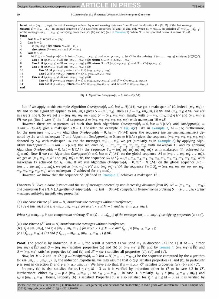
We denote the algorithm as OneApprox[dI = 0, last = D](M). For an ordered input sequence M of messages and the direction D ∈ {H, V }, it gives as output an ordered sequence S of the messages such that the basic scheme (S, last = D)
has makespan at most LB + 1. Algorithm OneApprox[dI = 0, last = D](M) is depicted in Fig. 5. As we explain in Remark 2, we can also obtain algorithms with the first message sent in direction D .
Example 3. Here, we give examples that illustrate the execution of Algorithm OneApprox. Moreover, we describe instances for which it is not optimal.
Consider again the Example of Fig. 4(a) (see Example 2). Let us apply Algorithm OneApprox[dI = 0, last = V ](M). First we apply the algorithm for m1, m2; (m1, m2) /∈ HV , we are at line 4 and S = (m2, m1) and S ′ = (m1). Then we consider m3, m4; the value of p (line 6) is m1; as (m1, m3) /∈ VH and (m2, m4) ∈ HV , we are in case 3.2 line 11 (p = mM−3). So we get, as O′ = (m1), S = (m1, m3, m2, m4). We now apply the algorithm with m5, m6; the value of p (line 6) is m4; as (m4, m5) /∈ VHand (m4, m6) /∈ HV , we are in case 4.1 line 13. So we get S = (m1, m3, m2, m4, m6, m5). The makespan of the algorithm is LB + 1 = 11 = d(m5) + 5 achieved for s6 = m5.
JID:TCS AID:9926 /FLA Doctopic: Algorithms, automata, complexity and games [m3G; v1.143-dev; Prn:6/11/2014; 9:19] P.10 (1-23)
10 J-C. Bermond et al. / Theoretical Computer Science ••• (••••) •••–•••
Input: M = (m1, . . . , mM ), the set of messages ordered by non-increasing distances from BS and the direction D ∈ {V , H} of the last message.Output: S = (s1, . . . , sM ) an ordered sequence of M satisfying properties (a) and (b) and, only when sM = mM−1, an ordering S ′ = (s′
1, . . . , s′M−1)
of the messages (m1, . . . , mM−1) satisfying properties (a’), (b’) and (c’) (see in Theorem 3). When S ′ is not specified below, it means S ′ = ∅.begin1 Case M = 1: return S = (m1)
2 Case M = 2:3 if (m1, m2) ∈ D̄D return S = (m1, m2)
4 else return S = (m2, m1) and S ′ = (m1)
5 Case M > 2:6 let O� p = OneApprox[dI = 0, last = D](m1, . . . , mM−2) and when p = mM−3, let O′ be the ordering of {m1, . . . , mM−3} satisfying (a’)(b’)(c’).7 Case 1: if (p, mM−1) ∈ DD̄ and (mM−1, mM ) ∈ D̄D return S = O � (p, mM−1, mM )
8 Case 2: if (p, mM−1) ∈ DD̄ and (mM−1, mM ) /∈ D̄D return S = O � (p, mM , mM−1) and S ′ = O � (p, mM−1)
9 Case 3: if (p, mM−1) /∈ DD̄ and (mM−2, mM ) ∈ D̄D10 Case 3.1: if p = mM−2 return S = O � (mM−1, mM−2, mM )
11 Case 3.2: if p = mM−3 return S = O′ � (mM−1, mM−2, mM )
12 Case 4: if (p, mM−1) /∈ DD̄ and (mM−2, mM ) /∈ D̄D13 Case 4.1: if p = mM−2 return S = O � (mM−2, mM , mM−1) and S ′ = O � (mM−1, mM−2)
14 Case 4.2: if p = mM−3 return S = O � (mM−3, mM , mM−1) and S ′ = O′ � (mM−1, mM−2)
end
Fig. 5. Algorithm OneApprox[dI = 0, last = D](M).
But, if we apply to this example Algorithm OneApprox[dI = 0, last = H](M), we get a makespan of 10. Indeed (m1, m2) ∈HV and so the algorithm applied to (m1, m2) gives S = (m1, m2). Then as p = m2, (m2, m3) ∈ HV and (m3, m4) /∈ VH, we are in case 2 line 8. So we get S = (m1, m2, m4, m3) and S ′ = (m1, m2, m3). Finally, with p = m3, (m3, m5) ∈ HV and (m5, m6) ∈VH we get (line 7 case 1) the final sequence S = (m1, m2, m4, m3, m5, m6) with makespan 10 = LB.
However there are sequences M such that both Algorithms OneApprox[dI = 0, last = V ](M) and OneApprox[dI =0, last = H](M) give a makespan LB + 1. Consider the example of Fig. 4(c). Like in Example 2, LB = 16; furthermore, for the messages m1, . . . , m6 Algorithm OneApprox[dI = 0, last = V ](M) gives the sequence (m1, m3, m2, m4, m6, m5) de-noted by S V with makespan 17 and Algorithm OneApprox[dI = 0, last = H](M) gives the sequence (m1, m2, m4, m3, m5, m6)
denoted by S H with makespan 16. For the messages m′1, . . . , m′
6, we get (similarly as in Example 2) by applying Algo-rithm OneApprox[dI = 0, last = V ](M) the sequence S ′
V = (m′1, m
′2, m
′4, m
′3, m
′5, m
′6) with makespan 10 and by applying
Algorithm OneApprox[dI = 0, last = H](M) the sequence S ′H = (m′
1, m′3, m
′2, m
′4, m
′6, m
′5) with makespan 11 achieved for
s′6 = m′
5. Now if we run Algorithm OneApprox[dI = 0, last = V ](M) on the global sequence M = (m1, . . . , m6, m′1, . . . , m
′6),
we get as (m5, m′1) ∈ VH and (m′
1, m′2) ∈ HV , the sequence S V � S ′
V = (m1, m3, m2, m4, m6, m5, m′1, m
′2, m
′4, m
′3, m
′5, m
′6) with
makespan 17 achieved for s6 = m5. If we run Algorithm OneApprox[dI = 0, last = H](M) on the global sequence M =(m1, . . . , m6, m′
1, . . . , m′6), we get as (m6, m′
1) ∈ HV and (m′1, m
′2) /∈ VH, the sequence S H � S ′
H = (m1, m2, m4, m3, m5, m6, m′1,
m′3, m
′2, m
′4, m
′6, m
′5) with makespan 17 achieved for s12 = m′
5.However, we know that the sequence S∗ (defined in Example 2) achieves a makespan 16.
Theorem 3. Given a basic instance and the set of messages ordered by non-increasing distances from BS, M = (m1, m2, . . . , mM)
and a direction D ∈ {H, V }, Algorithm OneApprox[dI = 0, last = D](M) computes in linear-time an ordering S = (s1, . . . , sM) of the messages satisfying the following properties:
(a) the basic scheme (S, last = D) broadcasts the messages without interference;(b) s1 ∈ {m1, m2} and si ∈ {mi−1, mi, mi+1} for any 1 < i ≤ M − 1, and sM ∈ {mM−1, mM}.
When sM = mM−1 , it also computes an ordering S ′ = (s′1, . . . , s
′M−1) of the messages (m1, . . . , mM−1) satisfying properties (a’)–(c’).
(a’) the scheme (S ′, last = D̄) broadcasts the messages without interference;(b’) s′
1 ∈ {m1, m2}, and s′i ∈ {mi−1, mi, mi+1} for any 1 < i ≤ M − 2, and s′
M−1 ∈ {mM−2, mM−1};
(c’) (s′M−1, mM) /∈ D̄D and if s′
M−1 = mM−2 , (mM−2, mM−1) /∈ DD̄.
Proof. The proof is by induction. If M = 1, the result is correct as we send m1 in direction D (line 1). If M = 2, either (m1, m2) ∈ D̄D and S = (m1, m2) satisfies properties (a) and (b) or (m1, m2) /∈ D̄D and by Lemma 1 (m2, m1) ∈ D̄D and S = (m2, m1) satisfies properties (a) and (b) and S ′ = (m1) satisfies all properties (a’), (b’) and (c’).
Now, let M > 2 and let O � p = OneApprox[dI = 0, last = D](m1, . . . , mM−2) be the sequence computed by the algorithm for (m1, m2, . . . , mM−2). By the induction hypothesis, we may assume that O� p satisfies properties (a) and (b). In particular p is sent in direction D and p ∈ {mM−3, mM−2}. We have also that, if p = mM−3, O′ satisfies properties (a’), (b’) and (c’).
Property (b) is also satisfied for si, 1 ≤ i ≤ M − 3 as it is verified by induction either in O or in case 3.2 in O′ . Furthermore, either sM−2 = p ∈ {mM−3, mM−2} or sM−2 = mM−1 in case 3. Similarly, sM−1 ∈ {mM−2, mM−1, mM} and sM ∈ {mM−1, mM}. Hence, Property (b) is satisfied. Property (b’) is also satisfied for s′, 1 ≤ i ≤ M − 3, as it is verified by
i
JID:TCS AID:9926 /FLA Doctopic: Algorithms, automata, complexity and games [m3G; v1.143-dev; Prn:6/11/2014; 9:19] P.11 (1-23)
J-C. Bermond et al. / Theoretical Computer Science ••• (••••) •••–••• 11
induction in O or for case 4.2 in O′ . Furthermore s′M−2 ∈ {mM−3, mM−2, mM−1} and s′
M−1 ∈ {mM−2, mM−1}. Hence, Prop-erty (b’) is satisfied.
Now let us prove that S satisfies property (a) and S ′ properties (a’) and (c’) in the six cases of the algorithm (lines 7–14). Obviously the last message in S (resp. S ′) is sent in direction D (resp. D̄).
In cases 1, 2, 3.1, 4.1 the hypothesis and sequence S are exactly the same as that given by Algorithm TwoApprox[dI =0, last = D](M). Therefore, by the proof of Theorem 1, S satisfies property (a) and so the proof is complete for cases 1 and 3.1 as there are no sequences S ′ .
In case 2, S ′ satisfies (a’) as by hypothesis (line 8) (p, mM−1) ∈ DD̄. Property (c’) is also satisfied as s′M−1 = mM−1 and by
hypothesis (line 8) (mM−1, mM) /∈ D̄D.In case 4.1 (p = mM−2), let q be the last element of O; (q, mM−2) ∈ D̄D as O � p is admissible. By hypothesis (line 12),
(mM−2, mM−1) /∈ DD̄ and then by Lemma 2 applied with q, mM−2, mM−1 in this order, we get (q, mM−1) ∈ D̄D; furthermore, by Lemma 1, (mM−2, mM−1) /∈ DD̄ implies (mM−1, mM−2) ∈ DD̄. So, S ′ satisfies Property (a’). Finally s′
M−1 = mM−2 and by hypothesis (line 12) (mM−2, mM) /∈ D̄D and (mM−2, mM−1) /∈ DD̄ and therefore S ′ satisfies property (c’).
The following claims are useful to conclude the proof in cases 3.2 and 4.2. In these cases p = mM−3 and let p′ be the last element of O′ . By induction on O′ , and by property (b’), p′ ∈ {mM−4, mM−3}.
Claim 1. In cases 3.2 and 4.2, (mM−2, mM−1) /∈ DD̄.
Proof. To write a convincing proof, we use coordinates and the expression of Fact 2 in terms of coordinates (see Remark 1). We use dest(mM−i) = (xM−i, yM−i). Let us suppose D = V (the claim can be proved for D = H by exchanging H and V and exchanging x and y).
By hypothesis (lines 9 and 12) (mM−3, mM−1) /∈ VH.
• If p′ = mM−3, by induction hypothesis (c’) applied to O′ , we have (p′, mM−2) /∈ HV . Then (mM−3, mM−1) /∈ VH and (mM−3, mM−2) /∈ HV imply by Fact 2: {xM−1 < xM−3 and yM−1 ≥ yM−3} and {xM−2 ≥ xM−3 and yM−2 < yM−3}.So we have xM−1 < xM−3 ≤ xM−2 implying xM−1 < xM−2 and yM−1 ≥ yM−3 > yM−2 implying yM−1 > yM−2. These conditions imply by Fact 2 that (mM−2, mM−1) /∈ VH.
• If p′ = mM−4, by induction hypothesis (c’) applied to O′ , we have (p′, mM−2) /∈ HV and (mM−4, mM−3) /∈ VH. So (mM−3, mM−1) /∈ VH, (mM−4, mM−2) /∈ HV and (mM−4, mM−3) /∈ VH imply respectively by Fact 2: {xM−1 < xM−3 and yM−1 ≥ yM−3}; {xM−2 ≥ xM−4 and yM−2 < yM−4} and {xM−3 < xM−4 and yM−3 ≥ yM−4}.So we have xM−1 < xM−3 < xM−4 ≤ xM−2 implying xM−1 < xM−2 and yM−1 ≥ yM−3 ≥ yM−4 > yM−2 implying yM−1 >
yM−2. These conditions imply by Fact 2 that (mM−2, mM−1) /∈ VH.
Claim 2. In cases 3.2 and 4.2, (p′, mM−1) ∈ D̄D.
Proof. If p′ = mM−3 by hypothesis lines 9 and 12 (mM−3, mM−1) /∈ DD̄ and by Lemma 1 (mM−3, mM−1) ∈ D̄D. If p′ = mM−4, by induction hypothesis (c’) applied to O′ , (mM−4, mM−3) /∈ DD̄ and so by Lemma 1 (mM−4, mM−3) ∈ D̄D; further-more by hypothesis (mM−3, mM−1) /∈ DD̄ and so by Lemma 2 applied with mM−4, mM−3, mM−1 in this order, we get (mM−4,mM−1) ∈ D̄D.
In case 3.2, by hypothesis (line 9) (mM−2, mM) ∈ D̄D; by the Claim 1 (mM−2, mM−1) /∈ DD̄ and so by Lemma 1(mM−1, mM−2) ∈ DD̄; and by Claim 2, (p′, mM−1) ∈ D̄D. So the theorem is proved in case 3.2.
Finally it remains to deal with the case 4.2. Let us first prove that S satisfies (a). By hypothesis line 12 (mM−2, mM) /∈D̄D and by the claim (mM−2, mM−1) /∈ DD̄ and so by Lemma 3 applied with mM−2, mM , mM−1 in this order we get (mM , mM−1) ∈ D̄D. We claim that (mM−3, mM−2) ∈ DD̄; indeed, if p′ = mM−3, by induction hypothesis (c’) applied to O′ , we have (mM−3, mM−2) /∈ D̄D and so (mM−3, mM−2) ∈ DD̄. If p′ = mM−4, by induction hypothesis (c’) applied to O′ , we have (mM−4, mM−2) /∈ D̄D and (mM−4, mM−3) /∈ DD̄ and so by Lemma 3 applied with mM−4, mM−3, mM−2 in this order we get (mM−3, mM−2) ∈ DD̄. Now the property (mM−3, mM−2) ∈ DD̄ combined with the hypothesis line 12 (mM−2, mM) /∈ D̄D gives by Lemma 2 applied with mM−3, mM−2, mM in this order (mM−3, mM) ∈ DD̄.
Finally, by Claim 1, (mM−2, mM−1) /∈ DD̄ and so by Lemma 1 (mM−1, mM−2) ∈ DD̄. By Claim 2, (p′, mM−1) ∈ D̄D and so S ′ satisfies Property (a’). S ′ satisfies also Property (c’) as (mM−2, mM) /∈ D̄D by hypothesis and (mM−2, mM−1) /∈ DD̄ by Claim 1. �
As corollary we get by property (b) and definition of LB that the basic scheme (S, last = D) achieves a makespan at most LB + 1. We emphasize this result as a Theorem and note that in view of Example 3 it is the best possible for the algorithm. The proof is similar to that Theorem 2.
Theorem 4. In the basic instance, the basic scheme (S, last = D) obtained by Algorithm OneApprox[dI = 0, last = D](M) achieves a makespan at most LB + 1.

JID:TCS AID:9926 /FLA Doctopic: Algorithms, automata, complexity and games [m3G; v1.143-dev; Prn:6/11/2014; 9:19] P.12 (1-23)
12 J-C. Bermond et al. / Theoretical Computer Science ••• (••••) •••–•••
As we have seen in Example 3, Algorithms OneApprox[dI = 0, last = V ](M) and OneApprox[dI = 0, last = H](M) are not always optimal since there are instances for which the optimal makespan equals LB while our algorithms only achieves LB + 1. However there are other cases where Algorithm OneApprox[dI = 0, last = V ](M) or Algorithm OneApprox[dI =0, last = H](M) can be used to obtain an optimal makespan LB. The next theorem might appear as specific, but it in-cludes the case where each node in a finite grid receives exactly one message (case considered in many papers in the literature, such as in [6] for the grid when buffering is allowed).
Theorem 5. Let M = (m1, m2, . . . , mM) be an ordered sequence of messages (i.e., by decreasing distance), if the bound LB =maxi≤M d(mi) + i − 1 is reached for an unique value of i, then we can design an algorithm with optimal makespan = LB.
Proof. Let k be the value for which LB is achieved that is d(mk) + k − 1 = LB and d(mi) + i − 1 < LB for i �= k. We divide M = (m1, . . . , mM) into two ordered subsequences Mk = (m1, . . . , mk) and M′
k = (mk+1, . . . , mM). So |Mk| = k and |M′k| =
M −k. Let SV (resp., SH ) be the sequence obtained by applying Algorithm OneApprox[dI = 0, last = V ](Mk) (resp., Algorithm OneApprox[dI = 0, last = H](Mk)) to the sequence Mk . The makespan is equal to LB; indeed if the sequence is (s1, . . . , sk), then the makespan is maxi≤k d(si) + i −1. But we have si ∈ {mi−1, mi, mi+1} for any i ≤ k −1, and so d(si) + i −1 ≤ d(mi−1) +(i −1) ≤ LB (as d(mi−1) + (i −1) −1 < LB); we also have sk ∈ {mk−1, mk} and so either d(sk) + (k −1) = d(mk−1) + (k −1) ≤ LBor d(sk) + (k − 1) = d(mk) + k − 1 = LB.
Suppose k > 1, then the destination of mk−1 is at the same distance of that of mk; indeed if d(mk−1) > d(mk), then d(mk−1) + k − 2 ≥ d(mk) + k − 1 = LB and LB is also achieved for k − 1 contradicting the hypothesis. Consider the set Dk of all the messages with destinations at the same distance as that of mk (so if k > 1 |Dk| ≥ 2) and let mu (resp., m�) be the uppermost message (resp., lowest message) of Dk , that is the message in Dk with destination the node with the highest y(resp., the lowest y); (in case there are many such messages with this property, i.e. they have the same destination node, we choose one of them).
We claim that there exists a basic scheme for Mk , such that if the last message is sent vertically (resp., horizontally) it is mu (resp. m�). Indeed, suppose we want the last message sent vertically to be mu it suffices to order the messages in Mk such that the last one mk = mu ; then if we apply Algorithm OneApprox[dI = 0, last = V ](Mk) we get a sequence where sk ∈ {mk−1, mk}. Either sk = mk = mu and we are done or sk = mk−1 and sk−1 = mu ; but in that case (sk−1, sk) ∈ HVimplies, by Fact 2, that xk−1 < xu or yk−1 ≥ yu , where (xu, yu) and (xk−1, yk−1) are the destinations of mu and mk−1. But mu, mk−1 ∈ Dk and mu being the uppermost vertex, yk−1 ≤ yu and xk−1 ≥ xu . Therefore, sk−1 and sk have the same destination. So, we can interchange them. Similarly using Algorithm OneApprox[dI = 0, last = H](Mk) we can obtain an HV-scheme denoted SH with the last message sent horizontally being m� .
If k=1, Mk is reduced to one message m1 and the claims are satisfied with mu = m� = m1 and SV = SH = m1.Now, we consider the sequence M′
k; the lower bound is LB′ = maxk<i≤M d(mi) + i − k − 1 < LB − k as LB is not achieved for any i �= k. Let S ′
H be the sequence obtained by applying Algorithm OneApprox[dI = 0, first = H](M′k) with the first
element of S ′H sent horizontally and let s′
h be this first element. (We obtain this algorithm from Algorithm OneApprox[dI =0, last = V ](M′
k) if |M ′k| = M − k is even or Algorithm OneApprox[dI = 0, last = H](M′
k) if |M ′k| is odd.) Similarly, let S ′
V be the sequence obtained by applying Algorithm OneApprox[dI = 0, first = V ](M′
k) with the first element of S ′V sent vertically
and let s′v be this first element. In all the cases the makespan is at most LB′ + 1 ≤ LB − k.
Finally, we consider the concatenation of the sequences SV �S ′H and SH �S ′
V . We claim that one of these two sequences has no interference. If the claim is true, then the theorem is proved as the makespan is LB for the first k messages and LB′ + 1 + k ≤ LB for the last M − k messages. In what follows, let as usual (xu, yu), (xl, yl), (x′
h, y′h) and (x′
v , y′v) denote
respectively the destinations of messages mu , ml , s′h and s′
v . Now, suppose the claim is not true, that is (mu, s′h) /∈ VH and
(m�, s′v) /∈ HV . That implies by Fact 2 that x′
h < xu and y′h ≥ yu and x′
v ≥ x� and y′v < y� . But we choose the destination of
mu (resp., m�) to be the uppermost one (resp., the lowest one) in Dk . So, xu ≤ xl and yu ≥ yl . Therefore x′h < x′
v and y′h > y′
vwhich imply first that s′
h �= s′v and by Fact 2 that (s′
v , s′h) /∈ VH and (s′
h, s′v) /∈ HV .
Note that, by the property of Algorithm OneApprox[dI = 0, last = D](M), s′h ∈ {mk+1, mk+2} and s′
v ∈ {mk+1, mk+2}; thus, as they are different, one of s′
h, s′v is mk+1 and the other mk+2. Suppose that s′
h = mk+1 and s′v = mk+2; then in the sequence
S ′V the first message is s′
v = mk+2 and from property (b) in Theorem 3, the second message is necessarily mk+1 = s′h , but
that implies (s′v , s′
h) ∈ VH a contradiction. The case s′h = mk+2 and s′
v = mk+1 implies similarly in the sequence S ′H that
(s′h, s′
v) ∈ HV , a contradiction. So the claim and the theorem are proved. �Example 4. As mentioned above, Algorithm OneApprox is not always optimal. The design of a polynomial-time optimal algorithm seems challenging because of some reasons that we discuss now. First, the first example below shows that there are open-grid instances for which any broadcast scheme using shortest paths in not optimal (a general grid with such property was already given in Example 1). In this example described in Fig. 6(a), we have 6 messages mi (1 ≤ i ≤ 6) with destinations at distance d for m1 and m2, d − 1 for m3 and d − 4 for m4, m5, m6. Here LB = d + 1, achieved for m2, m3and m6. In the Fig. 6(a), d = 14, v1 = (11, 3), v2 = (12, 2), v3 = (9, 4), v4 = (5, 5), v5 = (3, 7) and v6 = (2, 8) and LB = 15. If we apply OneApprox[dI = 0, last = V ](M) we get the sequence (m1, m3, m2, m5, m4, m6) with a makespan 16 attained for s3 = m2. If we apply OneApprox[dI = 0, last = H](M) we get the sequence (m1, m2, m4, m3, m6, m5) also with a makespan 16 attained for s4 = m3. Consider any algorithm where the messages are sent via shortest directed paths. If the makespan is LB then m1 and m2 should be sent in the first two steps and to avoid interference the source should send m1 via (0, 1) and

JID:TCS AID:9926 /FLA Doctopic: Algorithms, automata, complexity and games [m3G; v1.143-dev; Prn:6/11/2014; 9:19] P.13 (1-23)
J-C. Bermond et al. / Theoretical Computer Science ••• (••••) •••–••• 13
Fig. 6. Examples for optimal schedules are difficult to obtain.
m2 via (1, 0). m3 should be sent at step 3. If m2 was sent at step 1 and so m1 at step 2, then m3 should be sent at step 3via (1, 0) and interferes with m1. Therefore, the only possibility is to send m1 at step 1 via (0, 1), m2 at step 2 via (1, 0) and m3 at step 3 via (0, 1). But then at step 4, we cannot send any of m4, m5, m6 without interference. So the source does no transmission at step 4, but the last sent message is sent at step 7 and the makespan is d + 2 = LB + 1. However there exists a tricky schedule with makespan LB, but not with shortest directed paths routing. We sent m1 vertically, m2 horizontally, m3 vertically but m4 with a detour to introduce a delay of 2. More precisely, if v4 = (x4, y4), we send m4 horizontally till (x4 + 1, 0), then to (x4 + 1, 1) and (x4, 1) (the detour) and then vertically till (x4, y4). Finally we send m6 vertically at step 5and m5 horizontally at step 6. m4 has been delayed by two but the message arrives at time LB and there is no interference between the messages.
Secondly, even if we restrict ourselves to use shortest paths, the computation of an optimal schedule seems difficult. Indeed, the second example below illustrates the fact that optimal schedule may be very different compared to the non-increasing distance schedule. The example is described in Fig. 6(b). We have 8 messages mi (1 ≤ i ≤ 8) with destinations at v1 = (6, 6), v2 = (5, 6), v3 = (2, 7), v4 = (2, 6), v5 = (1, 5), v6 = (2, 4), v7 = (3, 2) and v8 = (4, 1). Here LB = 12, achieved for m1, m2 and m8. We prove that there is a unique sequence of messages reaching the bound LB which is the ordered se-quence (m1, m2, m6, m3, m4, m5, m8, m7) with the first message sent horizontally. Indeed to reach the makespan LB, m1 and m2 have to be sent first and second because their distances are 12 and 11 and in order they do not interfere m1 has to be sent horizontally and m2 vertically.The next message to be sent cannot be m3 nor m4 as they interfere with m2. If the third message sent is mi for some i ∈ 5,7,8, then the fourth and fifth messages have to be m3 vertically then m4 horizontally since their distances are 9 and 8. Now only message m5 can be sent vertically at step 6, otherwise there is interference with m4. Then message m6 has to be sent horizontally at step 7 since its distance is 6. But then the last message m7 or m8(the one not sent at the third step) can not be sent vertically as it interferes with m6. So the only possibility consists in sending m6 at the third step and then the ordered sequence is forced.
In the last example, some specific message (m6) has to be chosen to be sent early (while being close to BS compared with other messages) to achieve the optimal solution. Deciding of such “critical” message seems to be not easy. Hence it shows that the complexity of determining the value of the minimum makespan might be a difficult problem (even when considering only shortest path schedules).
4. Case dI = 0; general grid, and BS in the corner
We see in this section that, by generalizing the notion of basic scheme, Algorithm TwoApprox[dI = 0, last = D](M) also achieves a makespan at most LB + 2 in the case of a general grid, that is when the destinations of the messages can be on one or both axes and with BS in the corner. First we have to generalize the notions of horizontal transmissions for a destination node on Y-axis and vertical transmissions for a destination node on the X-axis. However the proofs of the basic lemmata are more complicated as Lemma 2 is not fully valid in this case. Furthermore, we cannot present the conditions only in simple terms like in Fact 2 and so to be precise we need to use coordinates.
JID:TCS AID:9926 /FLA Doctopic: Algorithms, automata, complexity and games [m3G; v1.143-dev; Prn:6/11/2014; 9:19] P.14 (1-23)
14 J-C. Bermond et al. / Theoretical Computer Science ••• (••••) •••–•••
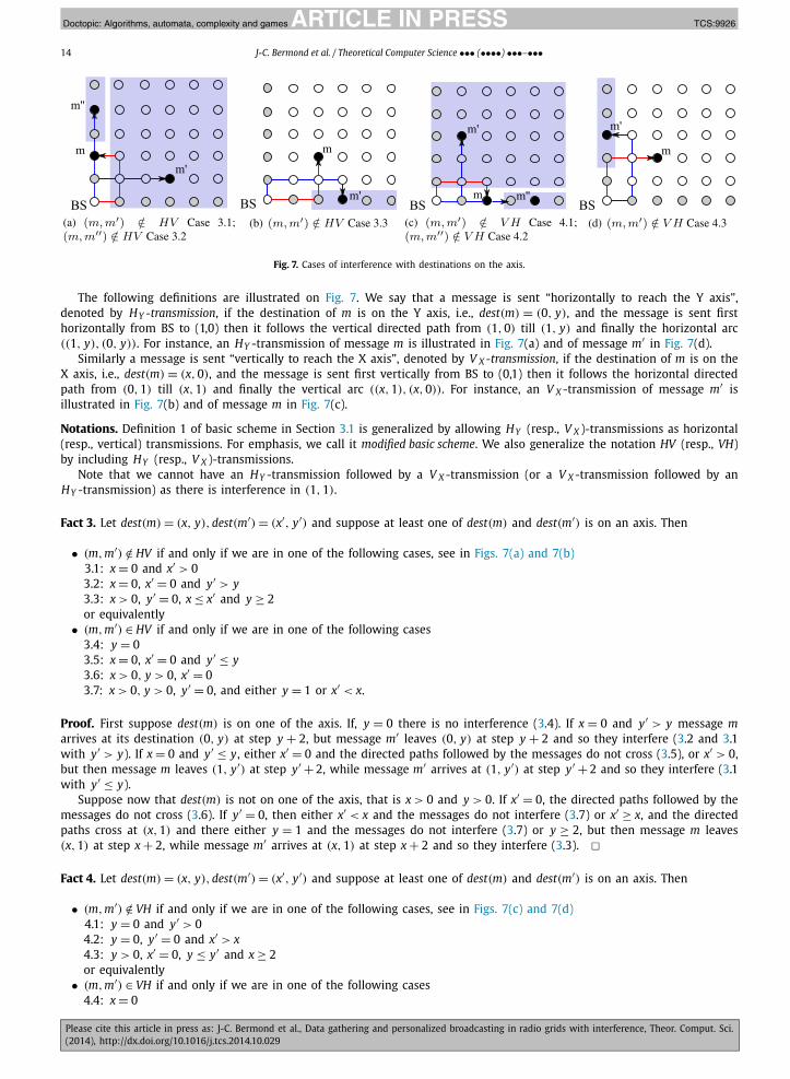
Fig. 7. Cases of interference with destinations on the axis.
The following definitions are illustrated on Fig. 7. We say that a message is sent “horizontally to reach the Y axis”, denoted by HY -transmission, if the destination of m is on the Y axis, i.e., dest(m) = (0, y), and the message is sent first horizontally from BS to (1,0) then it follows the vertical directed path from (1, 0) till (1, y) and finally the horizontal arc ((1, y), (0, y)). For instance, an HY -transmission of message m is illustrated in Fig. 7(a) and of message m′ in Fig. 7(d).
Similarly a message is sent “vertically to reach the X axis”, denoted by V X -transmission, if the destination of m is on the X axis, i.e., dest(m) = (x, 0), and the message is sent first vertically from BS to (0,1) then it follows the horizontal directed path from (0, 1) till (x, 1) and finally the vertical arc ((x, 1), (x, 0)). For instance, an V X -transmission of message m′ is illustrated in Fig. 7(b) and of message m in Fig. 7(c).
Notations. Definition 1 of basic scheme in Section 3.1 is generalized by allowing HY (resp., V X )-transmissions as horizontal (resp., vertical) transmissions. For emphasis, we call it modified basic scheme. We also generalize the notation HV (resp., VH) by including HY (resp., V X )-transmissions.
Note that we cannot have an HY -transmission followed by a V X -transmission (or a V X -transmission followed by an HY -transmission) as there is interference in (1, 1).
Fact 3. Let dest(m) = (x, y), dest(m′) = (x′, y′) and suppose at least one of dest(m) and dest(m′) is on an axis. Then
• (m, m′) /∈ HV if and only if we are in one of the following cases, see in Figs. 7(a) and 7(b)3.1: x = 0 and x′ > 03.2: x = 0, x′ = 0 and y′ > y3.3: x > 0, y′ = 0, x ≤ x′ and y ≥ 2or equivalently
• (m, m′) ∈ HV if and only if we are in one of the following cases3.4: y = 03.5: x = 0, x′ = 0 and y′ ≤ y3.6: x > 0, y > 0, x′ = 03.7: x > 0, y > 0, y′ = 0, and either y = 1 or x′ < x.
Proof. First suppose dest(m) is on one of the axis. If, y = 0 there is no interference (3.4). If x = 0 and y′ > y message marrives at its destination (0, y) at step y + 2, but message m′ leaves (0, y) at step y + 2 and so they interfere (3.2 and 3.1 with y′ > y). If x = 0 and y′ ≤ y, either x′ = 0 and the directed paths followed by the messages do not cross (3.5), or x′ > 0, but then message m leaves (1, y′) at step y′ + 2, while message m′ arrives at (1, y′) at step y′ + 2 and so they interfere (3.1 with y′ ≤ y).
Suppose now that dest(m) is not on one of the axis, that is x > 0 and y > 0. If x′ = 0, the directed paths followed by the messages do not cross (3.6). If y′ = 0, then either x′ < x and the messages do not interfere (3.7) or x′ ≥ x, and the directed paths cross at (x, 1) and there either y = 1 and the messages do not interfere (3.7) or y ≥ 2, but then message m leaves (x, 1) at step x + 2, while message m′ arrives at (x, 1) at step x + 2 and so they interfere (3.3). �Fact 4. Let dest(m) = (x, y), dest(m′) = (x′, y′) and suppose at least one of dest(m) and dest(m′) is on an axis. Then
• (m, m′) /∈ VH if and only if we are in one of the following cases, see in Figs. 7(c) and 7(d)4.1: y = 0 and y′ > 04.2: y = 0, y′ = 0 and x′ > x4.3: y > 0, x′ = 0, y ≤ y′ and x ≥ 2or equivalently
• (m, m′) ∈ VH if and only if we are in one of the following cases4.4: x = 0

JID:TCS AID:9926 /FLA Doctopic: Algorithms, automata, complexity and games [m3G; v1.143-dev; Prn:6/11/2014; 9:19] P.15 (1-23)
J-C. Bermond et al. / Theoretical Computer Science ••• (••••) •••–••• 15
4.5: y = 0, y′ = 0 and x′ ≤ x4.6: x > 0, y > 0, y′ = 04.7: x > 0, y > 0, x′ = 0, and either x = 1 or y′ < y.
Lemma 4. If (m, m′) /∈ DD̄, then (m, m′) ∈ D̄D and (m′, m) ∈ DD̄.
Proof. We prove that if (m, m′) /∈ HV (case D = H), then (m, m′) ∈ VH in the following. Other results are proved similarly. If none of the destinations of m and m′ are on the axis, the result holds by Lemma 1. If at least one destination is on an axis, suppose that (m, m′) /∈ HV . If conditions of Fact 3.1 or 3.2 are satisfied, then x = 0 but then by Fact 4.4 (m, m′) ∈ VH. If condition of Fact 3.3 is satisfied, so x > 0, y′ = 0 and y ≥ 2 which implies by Fact 4.6 that (m, m′) ∈ VH. �
However Lemma 2 is no more valid in its full generality.
Lemma 5. Let dest(m) = (x, y), dest(m′) = (x′, y′) and dest(m′′) = (x′′, y′′).If (m, m′) ∈ DD̄ and (m′, m′′) /∈ D̄D, then (m, m′′) ∈ DD̄ except if:
• Case D = H: y′ = 0 (V X -transmission is used for m′), and y ≥ max(2, y′′ + 1), and 0 < x′ < x ≤ x′′ .• Case D = V : x′ = 0 (HY -transmission is used for m′), and x ≥ max(2, x′′ + 1), and 0 < y′ < y ≤ y′′ .
Proof. Let us prove the case D = H . If none of the destinations of m, m′, m′′ are on an axis the result holds by Lemma 2. If y = 0, then (m, m′′) ∈ HV by Fact 3.4. By Fact 4, (m′, m′′) /∈ VH implies x′ > 0. If x = 0, then by Fact 3.5, (m, m′) ∈ HVimplies x′ = 0 a contradiction with the preceding assertion. Therefore x > 0 and dest(m) is not on an axis. If x′′ = 0, then by Fact 3.6 (m, m′′) ∈ HV . If y′ > 0, then (m′, m′′) /∈ VH implies x′′ = 0 by Fact 4.3, where we already know that by Fact 3.6 (m, m′′) ∈ HV . So y′ = 0, x > 0, y > 0 and by Fact 3.7 (m, m′) ∈ HV implies that either y = 1 or x′ < x.
If y′′ = 0, by Fact 3.3, (m, m′′) /∈ HV if and only if y ≥ 2 and x ≤ x′′ . If y′′ > 0, none of the destinations of m and m′′are on the axis and so by Fact 2, (m, m′′) /∈ HV , if and only if x′′ ≥ x and y′′ < y. So again y ≥ 2 and x ≤ x′′ . In summary (m, m′′) /∈ HV , if and only if y ≥ 2 and when y′′ > 0, y > y′′ and 0 < x′ < x ≤ x′′
The case D = V is obtained similarly. �We give the following useful corollary for the proof of the next theorem.
Corollary 1. If d(m′) ≥ d(m′′) then: If (m, m′) ∈ DD̄ and (m′, m′′) /∈ D̄D, then (m, m′′) ∈ DD̄.
We now show that:
Lemma 6. Lemma 3 is still valid in general grid.
Proof. We prove it for D = H . The case D = V can be obtained similarly.If none of the destinations of m, m′, m′′ are on an axis the result holds by Lemma 3. Suppose first dest(m′′) is on an axis;
by Fact 4 (m, m′′) /∈ VH implies x > 0. If furthermore dest(m) or dest(m′) are on an axis, by Fact 3.3 (m, m′) /∈ HV implies y′ = 0 and so by Fact 3.4 (m′, m′′) ∈ HV . Otherwise if none of dest(m) and dest(m′) are on an axis, y > 0 and by Fact 4.3 (m, m′′) /∈ VH implies x′′ = 0, and with x′ > 0 and y′ > 0 Fact 3.6 implies (m′, m′′) ∈ HV .
If dest(m′′) is not on an axis, then one of dest(m) and dest(m′) is on an axis and (m, m′) /∈ HV implies y > 0. We cannot have x = 0 otherwise it contradicts (m, m′′) /∈ VH. If x > 0, then by Fact 3.3 (m, m′) /∈ HV implies y′ = 0, but then Fact 3.4 implies (m′, m′′) ∈ HV . �Theorem 6. Let dI = 0, and BS be in the corner of the general grid. Given the set of messages ordered by non-increasing distances from BS, M = (m1, m2, . . . , mM) and a direction D, Algorithm TwoApprox[dI = 0, last = D](M) computes in linear-time an ordering Sof the messages satisfying following properties
(i) the modified basic scheme (S, last = D) broadcasts the messages without interference;(ii) s1 ∈ {m1, m2, m3}, s2 ∈ {m1, m2, m3, m4} and si ∈ {mi−2, mi−1, mi, mi+1, mi+2} for any 2 < i ≤ M − 2, and sM−1 ∈
{mM−3, mM−2, mM−1, mM} and sM ∈ {mM−1, mM};(iii) for any i ≤ M, if si is an HY (resp., V X ) transmission with destination on column 0 (resp., on line 0), then either si ∈
{mi, mi+1, mi+2} if i < M − 1, or si ∈ {mi, mi+1} if i = M − 1, or si = mi if i = M.
Proof. We prove the theorem for D = V . The case D = H can be proved similarly. The proof is by induction on M and follows the proof of Theorem 1. We have to verify the new property (iii) and property (i) when one of p, q, mM−1, mMhas its destination on one of the axis. Recall that q is the last message in O. We denote dest(p) = (xp, yp), and as usual dest(mM−1) = (xM−1, yM−1) and dest(mM) = (xM , yM).

JID:TCS AID:9926 /FLA Doctopic: Algorithms, automata, complexity and games [m3G; v1.143-dev; Prn:6/11/2014; 9:19] P.16 (1-23)
16 J-C. Bermond et al. / Theoretical Computer Science ••• (••••) •••–•••
For property (i) the proof of Theorem 1 works if, when using Lemma 2, we are in a case where it is still valid, that is when Lemma 5 is valid. We use Lemma 2 to prove case 2 of Algorithm TwoApprox[dI = 0, last = V ](M) with p, mM−1, mM
in this order. The order on the messages implies d(mM−1) ≥ d(mM) and so by Corollary 1, Lemma 5 is valid. We also use Lemma 2 to prove the case 3 of the algorithm with q, p, mM−1 in this order. The order on the messages implies d(p) ≥ d(mM−1) and so by Corollary 1, Lemma 5 is valid. Note that to prove case 4 of the algorithm we use Lemma 3 which is still valid (Lemma 6).
It remains to verify property (iii). In case 2 of the algorithm, we have to show that sM = mM−1 is not using V X -transmission because we use induction for (m1, . . . , mM−2). So it is sufficient to prove yM−1 > 0. Indeed, by Fact 3, (mM−1, mM) /∈ HV implies yM−1 > 0.
In case 3 of the algorithm, to verify property (iii) we have to show that sM−1 = p is not using HY -transmission because we use induction for (m1, . . . , mM−2). So it is sufficient to prove xp > 0. Indeed, by Fact 4, (p, mM−1) /∈ VH implies xp > 0.
In case 4 of the algorithm, to verify property (iii) we have to show that sM = mM−1 is not using V X -transmission. Suppose it is not the case i.e. yM−1 = 0; as (p, mM−1) /∈ VH, we have by Fact 4.2 yp = 0 and xM−1 > xp . But then d(p) <d(mM−1) contradicts the order of the messages. �
As corollary we get by properties (ii) and (iii) and the definition of LB, that the modified basic scheme (S, last = D)
achieves a makespan at most LB + 2. We emphasize this result as a Theorem and note that in view of Example 2 or the example given at the end of Section 2 it is the best possible.
Theorem 7. In the general grid with BS in the corner and dI = 0, the modified basic scheme (S, last = D) obtained by AlgorithmTwoApprox[dI = 0, last = D](M) achieves a makespan at most LB + 2.
5. dI -Open grid when dI ∈ {1, 2}
In this section, we use Algorithm OneApprox[dI = 0, last = D](M) and the detour similar with the one in Example 4 to solve the personalized broadcasting problem for dI ∈ {1, 2} in dI -open grids, defined as follows. The base station is in the corner throughout this section, i.e. it has coordinates (0, 0).
Definition 2. A grid with BS in the corner is called 1-open grid if at least one of the following conditions is satisfied: (1) All messages have destination nodes in the set {(x, y) : x ≥ 2 and y ≥ 1}; (2) All messages have destination nodes in the set {(x, y) : x ≥ 1 and y ≥ 2}.
The 1-open grid differs from the open grid only by excluding destinations of messages either on the line x = 1 (condi-tion (1)) or on the column y = 1 (condition (2)). For dI ≥ 2 the definition is simpler.
Definition 3. For dI ≥ 2, a grid with BS in the corner is called dI -open grid if all messages have destination nodes in the set {(x, y) : x ≥ dI and y ≥ dI }.
5.1. Lower bounds
In this subsection, we give the lower bounds of the makespan for dI ∈ {1, 2} in dI -open grids:
Proposition 2. Let G be a grid with BS in the corner, dI = 1 and the set of messages, M = (m1, m2, . . . , mM), ordered by non-increasing distances from BS, with all the destinations at distance at least 3 (d(mM) ≥ 3), then the makespan of any broadcasting scheme is greater than or equal to LBc(1) = maxi≤Md(mi) + 3i/2� − 2.
Proof. First we claim that if the source sends two messages in two consecutive steps t and t + 1, then it cannot send at step t + 2. Indeed, suppose that the source sends a message m at step t on one axis; then at step t + 1 it must send the message m′ on the other axis. But then at step t + 2, both the two neighbors of the source are at distance at most 1 from the sender of messages m or m′. So if the source sends m′′ at step t + 2, m′′ interferes with m or m′.
Let ti be the step where the last message in (m1, m2, . . . , mi) is sent; therefore ti ≥ 3i/2� − 1. This last mes-sage denoted m is received at step t′
i ≥ d(m) + ti − 1 ≥ d(mi) + ti − 1 ≥ d(mi) + 3i/2� − 2 and for every i ≤ M , LBc(1) ≥ d(mi) + 3i/2� − 2. �Remark 3. (A): Obviously, this bound is valid for 1-open grid according to Definition 2.
(B): This bound is valid for dI = 1 only when the source has a degree 2 (case BS in the corner of the grid). If BS is in a general position in the grid we have no better bound than LB.
(C): One can check that the bound is still valid if at most one message has a destination at distance 1 or 2. But if two or more messages have such destinations (d(mM−1) ≤ 2), then the bound is no more valid. As an example, let dest(mi) = vi ,
JID:TCS AID:9926 /FLA Doctopic: Algorithms, automata, complexity and games [m3G; v1.143-dev; Prn:6/11/2014; 9:19] P.17 (1-23)
J-C. Bermond et al. / Theoretical Computer Science ••• (••••) •••–••• 17
with v1 = (1, 2), v2 = (2, 1), v3 = (1, 2) and v4 = v5 = (1, 1), then d(m1) = d(m2) = d(m3) = 3 and d(m4) = d(m5) = 2 and LBc(1) = d(m5) + 6 = 8. However we can achieve a makespan of 7 by sending m4 horizontally at step 1, then m1 vertically at step 2 and m2 horizontally at step 3, then the source sends m3 vertically at step 5 and m5 horizontally at step 6. m3 and m5 reach their destinations at step 7.
(D): Finally let us also remark that there exist configurations for which no gathering protocol can achieve better makespan than LBc(1) + 1. Let dest(m1) = v1 = (x, y), with x + y = d, dest(m2) = v2 = (x, y − 1) and dest(m3) = v3 =(x − 1, y − 2). To achieve a makespan of LBc(1) = d, m1 should be sent at step 1 via a shortest directed path; m2 should be sent at step 2 via a shortest directed path; and m3 should be sent at step 4 via a shortest directed path. But, at step d, the sender of m2 (either (x, y − 2) or (x − 1, y − 1)) is at distance 1 from v3 = dest(m3) and so m2 and m3 interfere.
For dI ≥ 2, we have the following lower bound.
Proposition 3. Let dI ≥ 2 and suppose we are in dI -open grid. Let M = (m1, m2, . . . , mM) be the set of messages ordered by non-increasing distances from BS, then the makespan of any broadcasting scheme is greater than or equal to LB(dI ) = maxi≤Md(mi) +(i − 1)dI .
Proof. Indeed if a source sends a message at some step the next message has to be sent at least dI steps after. �Remark 4. For dI = 2, there exist configurations for which no gathering protocol can achieve a better makespan than LB(2) + 2. Let dest(m1) = v1 = (x, y), with x + y = d and dest(m2) = v2 = (x − 1, y − 1). Note that LB(2) = d. Let s1, s2 be the sequence obtained by some algorithm; to avoid interference s1 being sent at step 1, s2 should be sent at step ≥3. If s2 = m1, the makespan is at least d + 2; Furthermore, if m1 is not sent via a shortest directed path again the makespan is at least d + 2. So s1 = m1 is sent at step 1 via a shortest directed path. At step d the sender of m1 (either (x, y − 1) or (x − 1, y)) is at distance 1 from v2. Therefore, if m2 is sent at step 3 (resp., 4) it arrives at v2 (resp., at a neighbor of v2) at step d and so m2 interferes with m1. Thus, m2 can be sent in the best case at step 5 and arrives at step d + 2. In all the cases, the makespan of any algorithm is LB(2) + 2.
5.2. Routing with ε-detours
To design the algorithms for dI ∈ {1, 2}, we use the sequence S obtained by Algorithm OneApprox[dI = 0, first = D](M). First, as seen in the proof of lower bounds, the source no more sends a message at each step. Second, we need to send the messages via directed paths more complicated than horizontal or vertical transmissions; however we see that we can use relatively simple directed paths with at most 2 turns and simple detours. Let us define precisely such transmissions.
Definition 4. We say that a message to be sent to node (x, y) is sent vertically with an ε-detour, if it follows the directed path from BS to (0, y + ε), then from (0, y + ε) to (x, y + ε) and finally from (x, y + ε) to (x, y). Similarly a message to be sent to node (x, y) is sent horizontally with an ε-detour, if it follows the directed path from BS to (x + ε, 0), then from (x + ε, 0) to (x + ε, y) and finally from (x + ε, y) to (x, y).
Note that ε = 0 corresponds to a message sent horizontally (or vertically) as defined earlier (in that case we also say that the message is sent without detour). Note also that in the previous section we use directed paths with 1-detour but only to reach vertices on the axes which are now excluded, since we are in open grid. A message sent at step t with an ε-detour reaches its destination at step t +d(m) +2ε−1. We also note that the detours introduced here are slightly different from the one used in Example 4. They are simpler in the sense that they are doing only two turns and for the case ε = 1(1-detour) going backward only at the last step.
We design algorithms using the sequence obtained by Algorithm OneApprox[dI = 0, first = D](M) but we have to send some of the messages with a 1-detour. We first give some lemmata which characterize when two messages m and m′ inter-fere when dI = 1, but not interfere in the basic scheme that is when dI = 0, according to the detours of their transmissions. For that the following fact which gives precisely the arcs used by the messages is useful.
Fact 5.
• If dest(m) = (x, y) and m is sent horizontally at step t with an ε-detour (ε = 0 or 1) then it uses at step t + h the following arccase 1: ((h, 0), (h + 1, 0)) for 0 ≤ h < x + εcase 2: ((x + ε, h − (x + ε)), (x + ε, h + 1 − (x + ε)) for x + ε ≤ h < x + y + εcase 3: if ε = 1 ((x + 1, y), (x, y)) for h = x + y + 1
• If dest(m′) = (x′, y′) and m′ is sent vertically with an ε′-detour (ε′ = 0 or 1) at step t′ , then it uses at step t′ + h′ the following arccase 1’: ((0, h′), (0, h′ + 1)) for 0 ≤ h′ < y′ + ε′
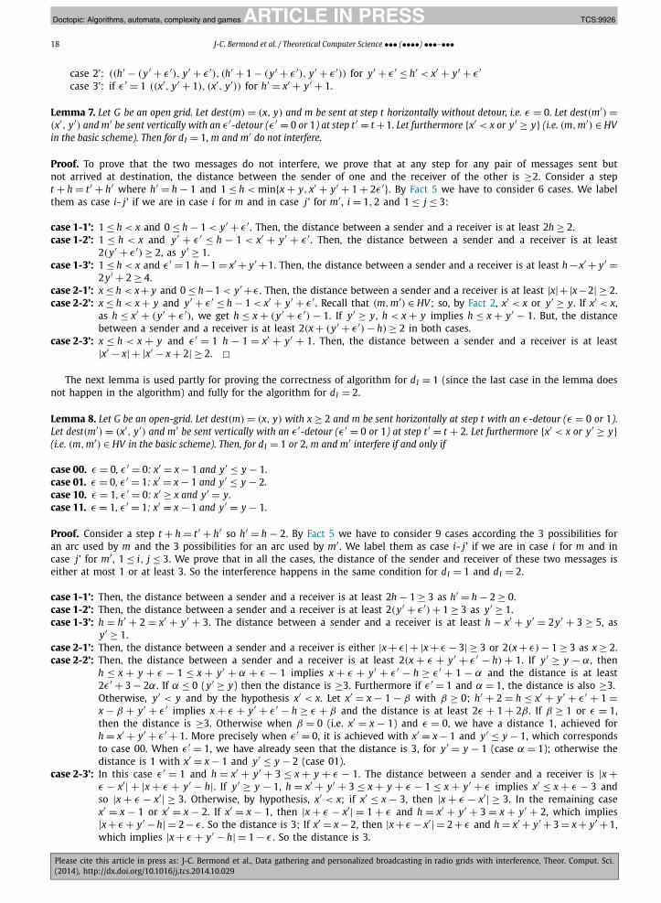
JID:TCS AID:9926 /FLA Doctopic: Algorithms, automata, complexity and games [m3G; v1.143-dev; Prn:6/11/2014; 9:19] P.18 (1-23)
18 J-C. Bermond et al. / Theoretical Computer Science ••• (••••) •••–•••
case 2’: ((h′ − (y′ + ε′), y′ + ε′), (h′ + 1 − (y′ + ε′), y′ + ε′)) for y′ + ε′ ≤ h′ < x′ + y′ + ε′case 3’: if ε′ = 1 ((x′, y′ + 1), (x′, y′)) for h′ = x′ + y′ + 1.
Lemma 7. Let G be an open grid. Let dest(m) = (x, y) and m be sent at step t horizontally without detour, i.e. ε = 0. Let dest(m′) =(x′, y′) and m′ be sent vertically with an ε′-detour (ε′ = 0 or 1) at step t′ = t +1. Let furthermore {x′ < x or y′ ≥ y} (i.e. (m, m′) ∈ HVin the basic scheme). Then for dI = 1, m and m′ do not interfere.
Proof. To prove that the two messages do not interfere, we prove that at any step for any pair of messages sent but not arrived at destination, the distance between the sender of one and the receiver of the other is ≥2. Consider a step t + h = t′ + h′ where h′ = h − 1 and 1 ≤ h < min{x + y, x′ + y′ + 1 + 2ε′}. By Fact 5 we have to consider 6 cases. We label them as case i- j’ if we are in case i for m and in case j’ for m′ , i = 1, 2 and 1 ≤ j ≤ 3:
case 1-1’: 1 ≤ h < x and 0 ≤ h − 1 < y′ + ε′ . Then, the distance between a sender and a receiver is at least 2h ≥ 2.case 1-2’: 1 ≤ h < x and y′ + ε′ ≤ h − 1 < x′ + y′ + ε′ . Then, the distance between a sender and a receiver is at least
2(y′ + ε′) ≥ 2, as y′ ≥ 1.case 1-3’: 1 ≤ h < x and ε′ = 1 h −1 = x′ + y′ +1. Then, the distance between a sender and a receiver is at least h − x′ + y′ =
2y′ + 2 ≥ 4.case 2-1’: x ≤ h < x + y and 0 ≤ h −1 < y′ +ε . Then, the distance between a sender and a receiver is at least |x| +|x −2| ≥ 2.case 2-2’: x ≤ h < x + y and y′ + ε′ ≤ h − 1 < x′ + y′ + ε′ . Recall that (m, m′) ∈ HV; so, by Fact 2, x′ < x or y′ ≥ y. If x′ < x,
as h ≤ x′ + (y′ + ε′), we get h ≤ x + (y′ + ε′) − 1. If y′ ≥ y, h < x + y implies h ≤ x + y′ − 1. But, the distance between a sender and a receiver is at least 2(x + (y′ + ε′) − h) ≥ 2 in both cases.
case 2-3’: x ≤ h < x + y and ε′ = 1 h − 1 = x′ + y′ + 1. Then, the distance between a sender and a receiver is at least |x′ − x| + |x′ − x + 2| ≥ 2. �
The next lemma is used partly for proving the correctness of algorithm for dI = 1 (since the last case in the lemma does not happen in the algorithm) and fully for the algorithm for dI = 2.
Lemma 8. Let G be an open-grid. Let dest(m) = (x, y) with x ≥ 2 and m be sent horizontally at step t with an ε-detour (ε = 0 or 1). Let dest(m′) = (x′, y′) and m′ be sent vertically with an ε′-detour (ε′ = 0 or 1) at step t′ = t + 2. Let furthermore {x′ < x or y′ ≥ y}(i.e. (m, m′) ∈ HV in the basic scheme). Then, for dI = 1 or 2, m and m′ interfere if and only if
case 00. ε = 0, ε′ = 0: x′ = x − 1 and y′ ≤ y − 1.case 01. ε = 0, ε′ = 1: x′ = x − 1 and y′ ≤ y − 2.case 10. ε = 1, ε′ = 0: x′ ≥ x and y′ = y.case 11. ε = 1, ε′ = 1: x′ = x − 1 and y′ = y − 1.
Proof. Consider a step t + h = t′ + h′ so h′ = h − 2. By Fact 5 we have to consider 9 cases according the 3 possibilities for an arc used by m and the 3 possibilities for an arc used by m′ . We label them as case i- j’ if we are in case i for m and in case j’ for m′ , 1 ≤ i, j ≤ 3. We prove that in all the cases, the distance of the sender and receiver of these two messages is either at most 1 or at least 3. So the interference happens in the same condition for dI = 1 and dI = 2.
case 1-1’: Then, the distance between a sender and a receiver is at least 2h − 1 ≥ 3 as h′ = h − 2 ≥ 0.case 1-2’: Then, the distance between a sender and a receiver is at least 2(y′ + ε′) + 1 ≥ 3 as y′ ≥ 1.case 1-3’: h = h′ + 2 = x′ + y′ + 3. The distance between a sender and a receiver is at least h − x′ + y′ = 2y′ + 3 ≥ 5, as
y′ ≥ 1.case 2-1’: Then, the distance between a sender and a receiver is either |x + ε| + |x + ε − 3| ≥ 3 or 2(x + ε) − 1 ≥ 3 as x ≥ 2.case 2-2’: Then, the distance between a sender and a receiver is at least 2(x + ε + y′ + ε′ − h) + 1. If y′ ≥ y − α, then
h ≤ x + y + ε − 1 ≤ x + y′ + α + ε − 1 implies x + ε + y′ + ε′ − h ≥ ε′ + 1 − α and the distance is at least 2ε′ + 3 − 2α. If α ≤ 0 (y′ ≥ y) then the distance is ≥3. Furthermore if ε′ = 1 and α = 1, the distance is also ≥3.Otherwise, y′ < y and by the hypothesis x′ < x. Let x′ = x − 1 − β with β ≥ 0; h′ + 2 = h ≤ x′ + y′ + ε′ + 1 =x − β + y′ + ε′ implies x + ε + y′ + ε′ − h ≥ ε + β and the distance is at least 2ε + 1 + 2β . If β ≥ 1 or ε = 1, then the distance is ≥3. Otherwise when β = 0 (i.e. x′ = x − 1) and ε = 0, we have a distance 1, achieved for h = x′ + y′ + ε′ + 1. More precisely when ε′ = 0, it is achieved with x′ = x − 1 and y′ ≤ y − 1, which corresponds to case 00. When ε′ = 1, we have already seen that the distance is 3, for y′ = y − 1 (case α = 1); otherwise the distance is 1 with x′ = x − 1 and y′ ≤ y − 2 (case 01).
case 2-3’: In this case ε′ = 1 and h = x′ + y′ + 3 ≤ x + y + ε − 1. The distance between a sender and a receiver is |x +ε − x′| + |x + ε + y′ − h|. If y′ ≥ y − 1, h = x′ + y′ + 3 ≤ x + y + ε − 1 ≤ x + y′ + ε implies x′ ≤ x + ε − 3 and so |x + ε − x′| ≥ 3. Otherwise, by hypothesis, x′ < x; if x′ ≤ x − 3, then |x + ε − x′| ≥ 3. In the remaining case x′ = x − 1 or x′ = x − 2. If x′ = x − 1, then |x + ε − x′| = 1 + ε and h = x′ + y′ + 3 = x + y′ + 2, which implies |x + ε + y′ − h| = 2 − ε . So the distance is 3; If x′ = x − 2, then |x + ε − x′| = 2 + ε and h = x′ + y′ + 3 = x + y′ + 1, which implies |x + ε + y′ − h| = 1 − ε . So the distance is 3.

JID:TCS AID:9926 /FLA Doctopic: Algorithms, automata, complexity and games [m3G; v1.143-dev; Prn:6/11/2014; 9:19] P.19 (1-23)
J-C. Bermond et al. / Theoretical Computer Science ••• (••••) •••–••• 19
case 3-1’: Then, the distance between a sender and a receiver is at least 2x − 1 ≥ 3 as x ≥ 2.case 3-2’: In that case ε = 1 and h = x + y + 1 and h ≤ x′ + y′ + ε′ + 1. The distance between a sender and a receiver
is |x + y′ + ε′ + 2 − h| + |y′ + ε′ − y|. If x′ ≤ x − 1, h = x + y + 1 ≤ x′ + y′ + ε′ + 1 ≤ x + y′ + ε′ implies |x +y′ + ε′ + 2 − h| + y′ + ε′ − y ≥ 2 + 1 = 3. Otherwise x′ ≥ x, and, by hypothesis, y′ ≥ y; Let y′ = y + γ with γ ≥ 0. So x + y′ + ε′ = x + y + γ + ε′ = h − 1 + γ + ε′ implies |x + y′ + ε′ + 2 − h| + y′ + ε′ − y ≥ 2ε′ + 2γ + 1. If ε′ = 1 or γ ≥ 1, then the distance is at least 3; otherwise the distance is 1 and so we have interference if ε = 1, ε′ = 0, x′ ≥ x and y′ = y (case 10).
case 3-3’: Then, ε = 1, ε′ = 1 and h = x + y + 1 = x′ + y′ + 3. The distance between a sender and a receiver is either |x + 1 − x′| + |y′ − y| or |x − x′| + |y′ + 1 − y|. If y′ ≥ y, then h = x + y + 1 = x′ + y′ + 3 implies x ≥ x′ + 2 and the distance is 3. If y′ ≤ y − 1, then by hypothesis x′ ≤ x − 1 and x + y + 1 = x′ + y′ + 3 implies y′ = y − 1and x′ = x − 1. Then the distance is 1 we have interference. In summary, we have interference if ε = 1, ε ′ = 1, x′ = x − 1 and y′ = y − 1 (case 11). �
By exchanging horizontally and vertically, x and y and x′ and y′ in Lemma 7 and Lemma 8 we get the following two lemmata:
Lemma 9. Let G be open grid. Let dest(m) = (x, y) and m be sent vertically (without detour) at step t. Let dest(m′) = (x′, y′) and m′be sent horizontally with an ε′-detour (ε′ = 0 or 1) at step t′ = t + 1. Let furthermore {x′ ≥ x or y′ < y} (i.e. (m, m′) ∈ VH in the basic scheme). Then, for dI = 1, m and m′ do not interfere.
Lemma 10. let G be an open grid. Let dest(m) = (x, y) with y ≥ 2 and m be sent vertically at step t with an ε-detour (ε = 0 or 1). Let dest(m′) = (x′, y′) and m′ be sent horizontally with an ε′-detour (ε′ = 0 or 1) at step t′ = t + 2. Let furthermore {x′ ≥ x or y′ < y}(i.e. (m, m′) ∈ VH in the basic scheme). Then for dI = 1 or 2, m and m′ interfere if and only if
case 00. ε = 0, ε′ = 0: x′ ≤ x − 1 and y′ = y − 1.case 01. ε = 0, ε′ = 1: x′ ≤ x − 2 and y′ = y − 1.case 10. ε = 1, ε′ = 0: x′ = x and y′ ≥ y.case 11. ε = 1, ε′ = 1: x′ = x − 1 and y′ = y − 1.
5.3. General-scheme dI = 1
We have to define general-scheme by indicating not only the ordered sequence of messages S = (s1, . . . , sM) sent by the source, but also by specifying for each si the time ti at which the message si is sent and the directed path followed by the message si , in fact the direction Di and the εi -detour used for sending it. More precisely,
Definition 5. A general-scheme is defined as a sequence of M quadruples (si, ti, Di, εi), where the i-th message sent by the source is si . This message is sent at step ti in direction Di with an εi -detour.
Note that we send the messages alternatively horizontally and vertically in our algorithm. Therefore, we have only to specify the direction of the first (or last) message. We see in the next theorem that the sequence S obtained by the algorithm OneApprox[dI = 0, first = D](M) in Section 3 almost works when dI = 1. More precisely, we propose a scheme that sends the messages in the same order as in S . However, BS waits one step every three steps; i.e., the source sends two messages of the sequence S during two consecutive steps and then stops transmission for one step. Furthermore, a message must sometimes be sent with a detour to avoid interference. That is, the messages are sent without detours like in S , except that, if the first message is sent in direction D , an even message s2k+2 is sent in direction D̄ with a 1-detour if and only if without detour it would interfere with s2k+3.
Theorem 8. Let dI = 1, and let BS be in a corner of a 1-open grid. Let M = (m1, . . . , mM) be the set of messages ordered by non-increasing distances from BS and suppose that the destination v = (x, y) of any message satisfies {x ≥ 1, y ≥ 2} (condition (2) of 1-open grid). Let us define:
• S = (s1, . . . , sM) is the ordered sequence obtained by Algorithm OneApprox[dI = 0, first = H](M),• for any i = 2k + 1, 0 ≤ k ≤ �(M − 1)/2 , let ti = 3k + 1 Di = H and εi = 0,• for any i = 2k + 2, 0 ≤ k < �M/2 , let ti = 3k + 2, Di = V and ε2k+2 = 0 if s2k+2 does not interferes with s2k+3 for dI = 1,
otherwise ε2k+2 = 1.
Then the general-scheme defined by the sequence (si, ti, Di, εi)i≤M broadcasts the messages without interference for dI = 1 and the first message is sent in direction H.
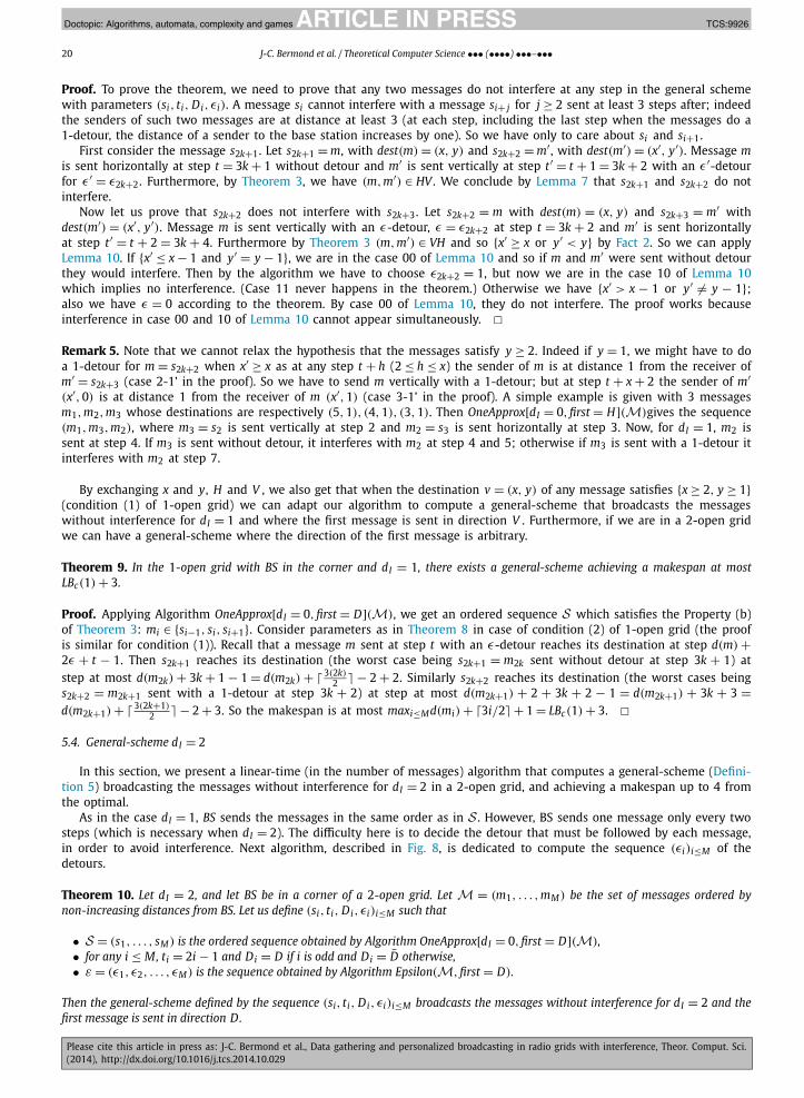
JID:TCS AID:9926 /FLA Doctopic: Algorithms, automata, complexity and games [m3G; v1.143-dev; Prn:6/11/2014; 9:19] P.20 (1-23)
20 J-C. Bermond et al. / Theoretical Computer Science ••• (••••) •••–•••
Proof. To prove the theorem, we need to prove that any two messages do not interfere at any step in the general scheme with parameters (si, ti, Di, εi). A message si cannot interfere with a message si+ j for j ≥ 2 sent at least 3 steps after; indeed the senders of such two messages are at distance at least 3 (at each step, including the last step when the messages do a 1-detour, the distance of a sender to the base station increases by one). So we have only to care about si and si+1.
First consider the message s2k+1. Let s2k+1 = m, with dest(m) = (x, y) and s2k+2 = m′ , with dest(m′) = (x′, y′). Message mis sent horizontally at step t = 3k + 1 without detour and m′ is sent vertically at step t′ = t + 1 = 3k + 2 with an ε′-detour for ε′ = ε2k+2. Furthermore, by Theorem 3, we have (m, m′) ∈ HV . We conclude by Lemma 7 that s2k+1 and s2k+2 do not interfere.
Now let us prove that s2k+2 does not interfere with s2k+3. Let s2k+2 = m with dest(m) = (x, y) and s2k+3 = m′ with dest(m′) = (x′, y′). Message m is sent vertically with an ε-detour, ε = ε2k+2 at step t = 3k + 2 and m′ is sent horizontally at step t′ = t + 2 = 3k + 4. Furthermore by Theorem 3 (m, m′) ∈ VH and so {x′ ≥ x or y′ < y} by Fact 2. So we can apply Lemma 10. If {x′ ≤ x − 1 and y′ = y − 1}, we are in the case 00 of Lemma 10 and so if m and m′ were sent without detour they would interfere. Then by the algorithm we have to choose ε2k+2 = 1, but now we are in the case 10 of Lemma 10which implies no interference. (Case 11 never happens in the theorem.) Otherwise we have {x′ > x − 1 or y′ �= y − 1}; also we have ε = 0 according to the theorem. By case 00 of Lemma 10, they do not interfere. The proof works because interference in case 00 and 10 of Lemma 10 cannot appear simultaneously. �Remark 5. Note that we cannot relax the hypothesis that the messages satisfy y ≥ 2. Indeed if y = 1, we might have to do a 1-detour for m = s2k+2 when x′ ≥ x as at any step t + h (2 ≤ h ≤ x) the sender of m is at distance 1 from the receiver of m′ = s2k+3 (case 2-1’ in the proof). So we have to send m vertically with a 1-detour; but at step t + x + 2 the sender of m′(x′, 0) is at distance 1 from the receiver of m (x′, 1) (case 3-1’ in the proof). A simple example is given with 3 messages m1, m2, m3 whose destinations are respectively (5, 1), (4, 1), (3, 1). Then OneApprox[dI = 0, first = H](M)gives the sequence (m1, m3, m2), where m3 = s2 is sent vertically at step 2 and m2 = s3 is sent horizontally at step 3. Now, for dI = 1, m2 is sent at step 4. If m3 is sent without detour, it interferes with m2 at step 4 and 5; otherwise if m3 is sent with a 1-detour it interferes with m2 at step 7.
By exchanging x and y, H and V , we also get that when the destination v = (x, y) of any message satisfies {x ≥ 2, y ≥ 1}(condition (1) of 1-open grid) we can adapt our algorithm to compute a general-scheme that broadcasts the messages without interference for dI = 1 and where the first message is sent in direction V . Furthermore, if we are in a 2-open grid we can have a general-scheme where the direction of the first message is arbitrary.
Theorem 9. In the 1-open grid with BS in the corner and dI = 1, there exists a general-scheme achieving a makespan at most LBc(1) + 3.
Proof. Applying Algorithm OneApprox[dI = 0, first = D](M), we get an ordered sequence S which satisfies the Property (b) of Theorem 3: mi ∈ {si−1, si, si+1}. Consider parameters as in Theorem 8 in case of condition (2) of 1-open grid (the proof is similar for condition (1)). Recall that a message m sent at step t with an ε-detour reaches its destination at step d(m) +2ε + t − 1. Then s2k+1 reaches its destination (the worst case being s2k+1 = m2k sent without detour at step 3k + 1) at step at most d(m2k) + 3k + 1 − 1 = d(m2k) + 3(2k)
2 � − 2 + 2. Similarly s2k+2 reaches its destination (the worst cases being s2k+2 = m2k+1 sent with a 1-detour at step 3k + 2) at step at most d(m2k+1) + 2 + 3k + 2 − 1 = d(m2k+1) + 3k + 3 =d(m2k+1) + 3(2k+1)
2 � − 2 + 3. So the makespan is at most maxi≤Md(mi) + 3i/2� + 1 = LBc(1) + 3. �5.4. General-scheme dI = 2
In this section, we present a linear-time (in the number of messages) algorithm that computes a general-scheme (Defini-tion 5) broadcasting the messages without interference for dI = 2 in a 2-open grid, and achieving a makespan up to 4 from the optimal.
As in the case dI = 1, BS sends the messages in the same order as in S . However, BS sends one message only every two steps (which is necessary when dI = 2). The difficulty here is to decide the detour that must be followed by each message, in order to avoid interference. Next algorithm, described in Fig. 8, is dedicated to compute the sequence (εi)i≤M of the detours.
Theorem 10. Let dI = 2, and let BS be in a corner of a 2-open grid. Let M = (m1, . . . , mM) be the set of messages ordered by non-increasing distances from BS. Let us define (si, ti, Di, εi)i≤M such that
• S = (s1, . . . , sM) is the ordered sequence obtained by Algorithm OneApprox[dI = 0, first = D](M),• for any i ≤ M, ti = 2i − 1 and Di = D if i is odd and Di = D̄ otherwise,• ε = (ε1, ε2, . . . , εM) is the sequence obtained by Algorithm Epsilon(M, first = D).
Then the general-scheme defined by the sequence (si, ti, Di, εi)i≤M broadcasts the messages without interference for dI = 2 and the first message is sent in direction D.

JID:TCS AID:9926 /FLA Doctopic: Algorithms, automata, complexity and games [m3G; v1.143-dev; Prn:6/11/2014; 9:19] P.21 (1-23)
J-C. Bermond et al. / Theoretical Computer Science ••• (••••) •••–••• 21
Input: M = (m1, . . . , mM ) the set of messages ordered by non-increasing distances from BS, in a 2-open grid, and the direction D of the first message.Output: ε = (ε1, ε2, . . . , εM ) where εi ∈ {0, 1}begin1 Let (s1, . . . , sM ) = OneApprox[dI = 0, first = D](M)
2 Let ti = 2i − 1, and Di = D if i is odd and Di = D̄ otherwise, for any 1 ≤ i ≤ M3 Let start with εi = 1 for 1 ≤ i ≤ M .4 for i = M − 1 to 15 if si interferes with si+1 in the general-scheme defined by (si, ti , Di , εi)i≤M when dI = 2 then
(we emphasis that we consider interference with the current values of the (εi)i≤M )6 εi ← 07 return ε = (ε1, ε2, . . . , εM )
end
Fig. 8. Algorithm Epsilon(M,first = D).
Proof. We need to prove that any two messages do not interfere at any step. A message si cannot interfere with a message si+ j , for j ≥ 2, sent at least 4 steps after. Indeed, at any step, the senders of two such messages are at distance at least 4. This is because, at each step including the last step when the messages do a 1-detour the distance of a sender to the base station increases by one. So we have only to show that si does not interfere with si+1 for any 1 ≤ i < M . For this purpose, we need the following claim that we prove thanks to Lemmas 8 and 10.
Claim 3. For dI = 2, if si sent with an εi = 1-detour interferes with si+1, then if we send si without detour, si does not interfere with si+1 .
Indeed suppose si is sent in direction D . As the sequence S is obtained by Algorithm OneApprox[dI = 0, first = D](M), (si, si+1) ∈ D D̄ . So we are in cases 10 if εi+1 = 0 or in case 11 if εi+1 = 1 of Lemma 8 (D = H) or Lemma 10 (D = V ). First suppose that we are in case 10, then we are not in the case 00; therefore if we send si without detour, si does not interfere with si+1. Now assume that we are in case 11, then we are not in the case 01; therefore if we send si without detour, si
does not interfere with si+1.Now Algorithm Epsilon(M, first = D) was designed in such a way it gives either εi = 1 in which case si does not interfere
with si+1 or it gives εi = 0 because si sent with a 1 detour was interfering with si+1, but then, by the Claim 3, si sent without detour does not interfere with si+1. �Theorem 11. In the 2-open grid with BS in the corner and dI = 2, the general-scheme defined in Theorem 10 achieves a makespan at most LB(2) + 4.
Proof. By definition of the scheme, the messages are sent in the same order as computed by OneApprox[dI = 0, first =D](M). Therefore, by Property (b) of Theorem 3, si ∈ {mi−1, mi, mi+1}. So the message si arrives at its destination at step d(si) + 2εi + ti − 1 ≤ d(mi−1) + 2 + 2i − 1 − 1 = d(mi−1) + 2(i − 1 − 1) + 4. Then the result follows from the definition of LB(2). �6. Personalized broadcasting in grid with arbitrary base station
In this section, we show how to use the algorithms proposed above to broadcast (or equivalently to gather) a set of personalized messages M, in a grid with a base station placed in an arbitrary node. More precisely, BS still has coordinates (0, 0), but the coordinates of the other nodes are in Z. A grid with arbitrary base station is said to be an open-grid if no destination nodes are on the axes. More generally, a grid with arbitrary base station is said to be an 2-open-grid if no destination nodes are at distance at most 1 from any axis.
We divide the grid into four quadrants Q q, 1 ≤ q ≤ 4, where Q 1 = {(x, y) such that x ≥ 0, y ≥ 0}, Q 2 = {(x, y) such that x ≤ 0, y ≥ 0}, Q 3 = {(x, y) such that x ≤ 0, y ≤ 0}, and Q 4 = {(x, y) such that x ≥ 0, y ≤ 0}. Note that, BS belongs to all quadrants, and any other node on an axis belongs to two different quadrants.
Each quadrant can be considered itself as a grid with the BS in the corner. Therefore, we can extend all the definitions of the preceding sections, in particular the basic scheme and general-scheme by considering a move in Q 1 (resp., Q 2, Q 3, Q 4) as horizontal, if it is on the positive x-axis (reps. positive y-axis, negative x-axis, negative y-axis) and a vertical move as one on the other half-axis of the quadrant. Then, if we have a sequence of consecutive messages, still ordered by non-increasing distance to BS, and all in the same quadrant we can apply any of the preceding algorithms. Otherwise, we can extend the algorithms by splitting the sequence of messages into maximal subsequences, where all the messages are in the same quadrant and applying any of the algorithms to this subsequence. We have just to be careful that there is no interference between the last message of a subsequence and the first one of the next subsequence; fortunately we take advantage of the fact that we can choose the direction of the first message of any subsequence.
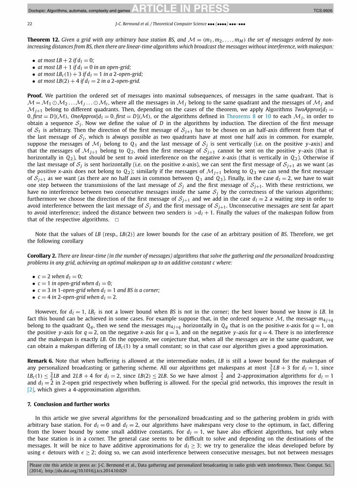
JID:TCS AID:9926 /FLA Doctopic: Algorithms, automata, complexity and games [m3G; v1.143-dev; Prn:6/11/2014; 9:19] P.22 (1-23)
22 J-C. Bermond et al. / Theoretical Computer Science ••• (••••) •••–•••
Theorem 12. Given a grid with any arbitrary base station BS, and M = (m1, m2, . . . , mM) the set of messages ordered by non-increasing distances from BS, then there are linear-time algorithms which broadcast the messages without interference, with makespan:
• at most LB + 2 if dI = 0;• at most LB + 1 if dI = 0 in an open-grid;• at most LBc(1) + 3 if dI = 1 in a 2-open-grid;• at most LB(2) + 4 if dI = 2 in a 2-open-grid.
Proof. We partition the ordered set of messages into maximal subsequences, of messages in the same quadrant. That is M =M1 �M2 . . .M j . . .�Mt , where all the messages in M j belong to the same quadrant and the messages of M j and M j+1 belong to different quadrants. Then, depending on the cases of the theorem, we apply Algorithms TwoApprox[dI =0, first = D](M), OneApprox[dI = 0, first = D](M), or the algorithms defined in Theorems 8 or 10 to each M j , in order to obtain a sequence S j . Now we define the value of D in the algorithms by induction. The direction of the first message of S1 is arbitrary. Then the direction of the first message of S j+1 has to be chosen on an half-axis different from that of the last message of S j , which is always possible as two quadrants have at most one half axis in common. For example, suppose the messages of M j belong to Q 1 and the last message of S j is sent vertically (i.e. on the positive y-axis) and that the messages of M j+1 belong to Q 2, then the first message of S j+1 cannot be sent on the positive y-axis (that is horizontally in Q 2), but should be sent to avoid interference on the negative x-axis (that is vertically in Q 2). Otherwise if the last message of S j is sent horizontally (i.e. on the positive x-axis), we can sent the first message of S j+1 as we want (as the positive x-axis does not belong to Q 2); similarly if the messages of M j+1 belong to Q 3 we can send the first message of S j+1 as we want (as there are no half axes in common between Q 1 and Q 3). Finally, in the case dI = 2, we have to wait one step between the transmissions of the last message of S j and the first message of S j+1. With these restrictions, we have no interference between two consecutive messages inside the same S j by the correctness of the various algorithms; furthermore we choose the direction of the first message of S j+1 and we add in the case dI = 2 a waiting step in order to avoid interference between the last message of S j and the first message of S j+1. Unconsecutive messages are sent far apart to avoid interference; indeed the distance between two senders is >dI + 1. Finally the values of the makespan follow from that of the respective algorithms. �
Note that the values of LB (resp., LB(2)) are lower bounds for the case of an arbitrary position of BS. Therefore, we get the following corollary
Corollary 2. There are linear-time (in the number of messages) algorithms that solve the gathering and the personalized broadcasting problems in any grid, achieving an optimal makespan up to an additive constant c where:
• c = 2 when dI = 0;• c = 1 in open-grid when dI = 0;• c = 3 in 1-open-grid when dI = 1 and BS is a corner;• c = 4 in 2-open-grid when dI = 2.
However, for dI = 1, LBc is not a lower bound when BS is not in the corner; the best lower bound we know is LB. In fact this bound can be achieved in some cases. For example suppose that, in the ordered sequence M, the message m4 j+qbelong to the quadrant Q q , then we send the messages m4 j+q horizontally in Q q that is on the positive x-axis for q = 1, on the positive y-axis for q = 2, on the negative x-axis for q = 3, and on the negative y-axis for q = 4. There is no interference and the makespan is exactly LB. On the opposite, we conjecture that, when all the messages are in the same quadrant, we can obtain a makespan differing of LBc(1) by a small constant; so in that case our algorithm gives a good approximation.
Remark 6. Note that when buffering is allowed at the intermediate nodes, LB is still a lower bound for the makespan of any personalized broadcasting or gathering scheme. All our algorithms get makespans at most 3
2 LB + 3 for dI = 1, since LBc(1) ≤ 3
2 LB and 2LB + 4 for dI = 2, since LB(2) ≤ 2LB. So we have almost 32 and 2-approximation algorithms for dI = 1
and dI = 2 in 2-open grid respectively when buffering is allowed. For the special grid networks, this improves the result in [2], which gives a 4-approximation algorithm.
7. Conclusion and further works
In this article we give several algorithms for the personalized broadcasting and so the gathering problem in grids with arbitrary base station. For dI = 0 and dI = 2, our algorithms have makespans very close to the optimum, in fact, differing from the lower bound by some small additive constants. For dI = 1, we have also efficient algorithms, but only when the base station is in a corner. The general case seems to be difficult to solve and depending on the destinations of the messages. It will be nice to have additive approximations for dI ≥ 3; we try to generalize the ideas developed before by using ε detours with ε ≥ 2; doing so, we can avoid interference between consecutive messages, but not between messages

JID:TCS AID:9926 /FLA Doctopic: Algorithms, automata, complexity and games [m3G; v1.143-dev; Prn:6/11/2014; 9:19] P.23 (1-23)
J-C. Bermond et al. / Theoretical Computer Science ••• (••••) •••–••• 23
si and si+2. Another challenging problem consists in determining the complexity of finding an optimal schedule and routing of messages for achieving the gathering in the minimum completion time or characterizing when the lower bound is achieved. Example 4 shows it might not be an easy problem. Determining if there is a polynomial algorithm to compute the makespan in the restricted case where messages should be sent via shortest directed paths seems also to be a challenging problem (see Example 4). Last but not least, a natural extension will be to consider the gathering problem for other network topologies.
Acknowledgements
We thank all referees for their very helpful comments.
References
[1] J.-C. Bermond, R. Correa, M.-L. Yu, Optimal gathering protocols on paths under interference constraints, Discrete Math. 309 (18) (September 2009) 5574–5587.
[2] J.-C. Bermond, J. Galtier, R. Klasing, N. Morales, S. Pérennes, Hardness and approximation of gathering in static radio networks, Parallel Process. Lett. 16 (2) (2006) 165–183.
[3] J.-C. Bermond, L. Gargano, S. Pérennes, A.A. Rescigno, U. Vaccaro, Optimal time data gathering in wireless networks with omni-directional antennas, in: SIROCCO 2011, in: Lecture Notes in Computer Science, vol. 6796, Springer-Verlag, Gdansk, Poland, June 2011, pp. 306–317.
[4] J.-C. Bermond, L. Gargano, A.A. Rescigno, Gathering with minimum completion time in sensor tree networks, J. Interconnect. Networks 11 (1–2) (2010) 1–33.
[5] J.C. Bermond, N. Nisse, P. Reyes, H. Rivano, Minimum delay data gathering in radio networks, in: Proceedings of the 8th International Conference on Ad Hoc Networks and Wireless (AdHoc-Now), in: Lecture Notes in Computer Science, vol. 5793, Springer, 2009, pp. 69–82.
[6] J.-C. Bermond, J. Peters, Optimal gathering in radio grids with interference, Theoret. Comput. Sci. 457 (October 2012) 10–26.[7] J.-C. Bermond, M.-L. Yu, Optimal gathering algorithms in multi-hop radio tree networks with interferences, Ad Hoc Sens. Wirel. Networks 9 (1–2)
(2010) 109–128.[8] P. Bertin, J.-F. Bresse, B. Le Sage, Accès haut débit en zone rurale: une solution “ad hoc”, France Telecom R&D 22 (2005) 16–18.[9] V. Bonifaci, R. Klasing, P. Korteweg, A. Marchetti-Spaccamela, L. Stougie, Data gathering in wireless networks, in: A. Koster, X. Munoz (Eds.), Graphs
and Algorithms in Communication Networks, Springer, Heidelberg, 2010, pp. 357–377.[10] V. Bonifaci, P. Korteweg, A. Marchetti Spaccamela, L. Stougie, An approximation algorithm for the wireless gathering problem, Oper. Res. Lett. 36 (5)
(2008) 605–608.[11] C. Florens, M. Franceschetti, R. McEliece, Lower bounds on data collection time in sensory networks, IEEE Journal on Selected Areas in Communications
22 (6) (2004) 1110–1120.[12] L. Gargano, A. Rescigno, Optimally fast data gathering in sensor networks, Discrete Appl. Math. 157 (2009) 1858–1872.[13] C. Gomes, S. Perennes, P. Reyes, H. Rivano, Bandwidth allocation in radio grid networks, in: Algotel’08, Saint Malo, May 2008.[14] R. Klasing, Z. Lotker, A. Navarra, S. Pérennes, From balls and bins to points and vertices, Algorithmic Oper. Res. 4 (2) (2009) 133–143.[15] Y. Revah, M. Segal, Improved algorithms for data-gathering time in sensor networks ii: ring, tree and grid topologies, in: Third International Conference
on Networking and Services, 2007 ICNS, 2007, p. 46.[16] Y. Revah, M. Segal, Improved bounds for data-gathering time in sensor networks, Comput. Commun. 31 (17) (2008) 4026–4034.[17] Y. Revah, M. Segal, L. Yedidsion, Real-time data gathering in sensor networks, Discrete Appl. Math. 158 (5) (2010) 543–550.[18] X. Zhu, B. Tang, H. Gupta, Delay efficient data gathering in sensor network, in: X. Jia, J. Wu, Y. He (Eds.), Proc. of MSN’05, in: Lecture Notes in Computer
Science, vol. 3794, Springer-Verlag, 2005, pp. 380–389.