data compression in distributed learning

Data Compression in Distributed Learning

Ming YanMichigan State University, CMSE/Mathematics

Computational Imaging

Institute for Mathematics and its ApplicationsOct. 14th, 2019

Ming Yan (MSU) DORE-1

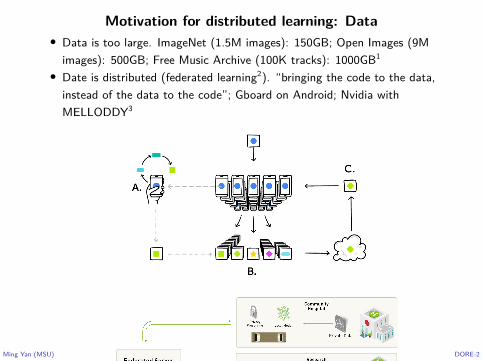
Motivation for distributed learning: Data• Data is too large. ImageNet (1.5M images): 150GB; Open Images (9M

images): 500GB; Free Music Archive (100K tracks): 1000GB1

• Date is distributed (federated learning2). “bringing the code to the data,instead of the data to the code”; Gboard on Android; Nvidia withMELLODDY3

1https://www.analyticsvidhya.com/blog/2018/03/comprehensive-collection-deep-learning-datasets/2https://ai.googleblog.com/2017/04/federated-learning-collaborative.html3https://blogs.nvidia.com/blog/2019/10/13/what-is-federated-learning/


Challenges in distributed learning

• Computation: floating point operations (FLOPS)• How does the computing cost of distributed learning compare with

centralized computing?• How to apply distributed learning on cellphones and other small

devices?• Communication: bandwidth (number of bits transferred) + latency

(rounds of communications)• latency � bandwidth � FLOPS• many new issues: synchronization, delay

• Other issues such as memory etc.


Outline

Communication in distributed learning

The intuition behind different quantization/compression techniques

DOuble REsidual compression algorithm (DORE)

Numerical experiments


The cost of communication4

execute typical instruction 1/1,000,000,000 sec = 1 nanosecfetch from L1 cache memory 0.5 nanosecfetch from L2 cache memory 7 nanosecfetch from main memory 100 nanosecsend 2K bytes over 1Gbps network 20,000 nanosecread 1MB sequentially from memory 250,000 nanosecread 1MB sequentially from disk 20,000,000 nanosecsend packet US to Europe and back 150 milliseconds = 150,000,000 nanosec

4https://norvig.com/21-days.htmlMing Yan (MSU) DORE-4

Approaches to reduce communication cost in SGD

• Reduce communication rounds• accelerated algorithms (which reduces the number of iterations)• more local updates, skip communication for small changes

• Reduce the communicated bits• Structured update: sparse, low rank. It works for special problems.• Data compression: topK (Stich et al., 2018; Aji-Heafield, 2017;

deterministic), QSGD (Alistarh et al. 17’; unbiased); Terngrad (Wenet al. 17’; unbiased); DIANA(Mishchenko et al. 19’; unbiased),1bit-SGD (Seide et al. 14’, Bernstein et al. 18’; deterministic), . . . .


Distributed learning problem we considered

• Optimization problem

minimizex∈Rp

f(x) +R(x) = 1n

n∑i=1

Eξ∼Di [`(x, ξ)]︸︷︷︸:=fi(x)

+R(x),

We mainly focus on the case R(x) = 0 in this talk.• Examples:• empirical risk minimization in statistical and machine learning• computer vision• image processing (deep learning)


Distributed structure

f(x)

Sensors 2017, 17, 2172 4 of 17

Figure 1. The first-generation parameter server system

The model uses a distributed Memcached to store the parameters, where each worker node only retains part of the parameters which are required in computing, and they can synchronize global model parameters with each other in this model. However, this parameter server is only a prototype design, the communication overhead is not optimized, and it is not suitable for distributed machine learning.

Industry has done a lot of work in improving the Parameter Server System. Dean et al. proposed a second-generation parameter server system in 2012, and developed a deep learning system called DistBelief [12] based on the Parameter Server System. As shown in Figure 2, the system sets up a global parameter server. The deep learning model is distributed stored on worker nodes, the communication between worker nodes is not allowed, and the PS is responsible for the transfer of all parameters. The second-generation parameter server system can solve the problem that the machine learning algorithms are very difficult to be distributed, but because it does not consider the performance differences of each worker node, the utilization of each worker node in the distributed system is still not high.

Figure 2. The second-generation parameter server system

Li proposed a third-generation parameter server system in 2014 [30,31]. As shown in Figure 3, the Parameter Server System provides a more general design, including a parameter server group and multiple worker nodes.

Training data

Workergroup

Servergroup

A worker node

Task schedule

r

Resource manager

Server manager

A server node

x

Parameter server/master node

Duplicated models

Data shards

• Data is partitioned at different nodes.• Each worker node sends the gradient to the master node.• The master node updates the model x and sends to the worker nodes.


Outline






Simple compression does not work

• Assume that all nodes have the true solution x∗. Then one step of parallel(exact) gradient descent with compression will leave x∗ in general.• That is

x = x∗ − γ

n

n∑i=1

Q(∇fi(x∗))

= x∗ − γ

n

n∑i=1

∇fi(x∗) + γ

n

n∑i=1

(∇fi(x∗)−Q(∇fi(x∗))).

The only ways to have x = x∗ are that the sum of the compression error is0 or γ = 0.


Simple compression with diminishing stepsize

• Because of the randomness in the gradient, SGD does not converge with aconstant stepsize generally.• A diminishing stepsize is used for convergence, and the convergence rate is

slower than gradient descent.• With a diminishing stepsize and unbiased compression, SGD converges

under the assumption that the stochastic gradient is bounded. (Combiningthe compression error into the randomness of the stochastic gradient.)• The convergence depends on the upper bound of the stochastic gradient.


Error compensation does not work• Main idea: add the compression error to the next variable to be

compressed (Seide et al. 14’; Wu et al. 18’; Stich et al. 18’; Karimireddyet al. 19’).

g = Q(g + e), e = (g + e)− g.• Assume that all nodes have the true solution x∗ at certain iteration. In

general, we have.

x = x∗ − γ

n

n∑i=1

Q(∇fi(x∗) + ei)

= x∗ − γ

n

n∑i=1

∇fi(x∗)

+ γ

n

n∑i=1

(∇fi(x∗) + ei −Q(∇fi(x∗) + ei))−γ

n

n∑i=1

ei.

The only ways to have x = x∗ are that the sum of the compression errordoes not change or γ = 0.• Its convergence with a diminishing stepsize also, and it requires the

boundedness of the stochastic gradient.Ming Yan (MSU) DORE-10

Difference quantization works

• Main idea: quantize the difference between the gradient and an estimation(Mishchenko et al. 19’; Li et al. 19’).• Assume that all nodes have the true solution x∗ at certain iteration. In

general, we have.

x = x∗ − γ

n

n∑i=1

hi +Q(∇fi(x∗)− hi)

= x∗ − γ

n

n∑i=1

∇fi(x∗) + γ

n

n∑i=1

(∇fi(x∗)− hi −Q(∇fi(x∗ − hi)))

• For a positive γ, if we can have hi = ∇fi(x∗), then we have x = x∗.• Question: How to update hi?


Outline






Additional considerations at the master node

• The previous compression only happens at the worker nodes, and thecommunication from the worker nodes to the master node is reduced.• Question: How to reduce the communication from the master node to the

worker nodes?• Question: If the sum of the compression error converges to 0, can we add

error compensation to increase the speed?



• The worker nodes send the compressed gradient residual to the masternode.• The master node broadcast the compressed model residual (the update of

the model) to the worker nodes.


DORE: AlgorithmInput: Stepsize α, β, γ, η, initialize h0 = h0

i = 0d, x0i = x0, ∀i ∈ {1, . . . , n}.

for k = 1, 2, · · · ,K − 1 do

For each worker {i = 1, 2, · · · , n}:

Sample gki such that E[gki |xki ] = ∇fi(xki )Gradient residual: ∆k

i = gki − hkiCompression: ∆k

i = Q(∆ki )

hk+1i = hki + α∆k

i

{ gki = hki + ∆ki }

Sent ∆ki to the master

Receive qk from the masterxk+1i = xki + βqk

For the master:

Receive ∆ki s from workers

∆k = 1/n∑n

i∆ki

gk = hk + ∆k{= 1n

∑n

igki }

hk+1 = hk + α∆k

qk = −γgk + ηek

Compression: qk = Q(qk)ek+1 = qk − qk

Broadcast qk to workersend forOutput: any xKi

• The worker nodes compress the residual.• The master node use error compensation and broadcasts the compressed

update (which converges to 0).


DORE with R(x)Input: Stepsize α, β, γ, η, initialize h0 = h0

i = 0d,x0i = x0, ∀i ∈ {1, . . . , n}.

for k = 1, 2, · · · ,K − 1 do

For each worker i ∈ {1, 2, · · · , n}:

Sample gki such that E[gki |xki ] = ∇fi(xki )Gradient residual: ∆k

i = gki − hkiCompression: ∆k

i = Q(∆ki )

hk+1i = hki + α∆k

i

{ gki = hki + ∆ki }

Send ∆ki to the master

Receive qk from the masterxk+1i = xki + βqk

For the master:

Receive {∆ki } from workers

∆k = 1/n∑n

i∆ki

gk = hk + ∆k{= 1n

∑n

igki }

xk+1 = proxγR(xk − γgk)hk+1 = hk + α∆k

Model residual: qk = xk+1−xk + ηek

Compression: qk = Q(qk)ek+1 = qk − qk

xk+1 = xk + βqk

Broadcast qk to workersend forOutput: xK or any xKi


Assumptions on the compressionAssumptionThe stochastic compression operator Q : Rd → Rd is unbiased, i.e., EQ(x) = xand satisfies

E‖Q(x)− x‖2 ≤ C‖x‖2,

for a nonnegative constant C that is independent of x.

• No Compression: C = 0 when there is no compression.• Stochastic Quantization: A real number x ∈ [a, b], (a < b) is set to be a

with probability b−xb−a and b with probability x−a

b−a , where a and b arepredefined quantization levels (QSGD). It satisfies when ab > 0.• Stochastic Sparsification: A real number x is set to be 0 with probability

1− p and xp

with probability p (Terngrad). It satisfies with C = (1/p)− 1.• p-norm Quantization: A vector x is quantized element-wisely byQp(x) = ‖x‖p sign(x) ◦ ξ, where ◦ is the Hadamard product and ξ is aBernoulli random vector satisfying ξi ∼ Bernoulli( |xi|‖x‖p ). It satisfies withC = maxx∈Rd

‖x‖1‖x‖p‖x‖2

2− 1.


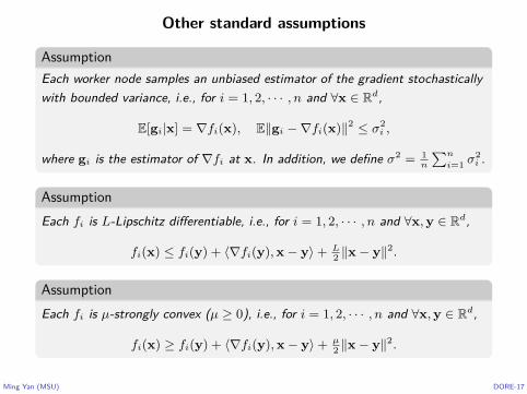
Other standard assumptions

AssumptionEach worker node samples an unbiased estimator of the gradient stochasticallywith bounded variance, i.e., for i = 1, 2, · · · , n and ∀x ∈ Rd,

E[gi|x] = ∇fi(x), E‖gi −∇fi(x)‖2 ≤ σ2i ,

where gi is the estimator of ∇fi at x. In addition, we define σ2 = 1n

∑n

i=1 σ2i .

AssumptionEach fi is L-Lipschitz differentiable, i.e., for i = 1, 2, · · · , n and ∀x,y ∈ Rd,

fi(x) ≤ fi(y) + 〈∇fi(y),x− y〉+ L2 ‖x− y‖2.

AssumptionEach fi is µ-strongly convex (µ ≥ 0), i.e., for i = 1, 2, · · · , n and ∀x,y ∈ Rd,

fi(x) ≥ fi(y) + 〈∇fi(y),x− y〉+ µ2 ‖x− y‖2.


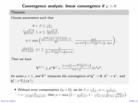
Convergence analysis: linear convergence if µ > 0TheoremChoose parameters such that

0 < β ≤ 1C+1

1−√

1−δ2(C+1) ≤ α ≤ 1+

√1−δ

2(C+1) ,

η < min(√

C2+4(1−(C+1)β)−C2C , 4µL

(µ+L)2(

1+ 4C(C+1)nδ

α)−4µL

),

η(µ+L)2(1+η)µL ≤γ ≤

2(1+ 4C(C+1)

nδα)

(µ+L).

Then we have

Vk+1 ≤ ρkV1 +(1+η)

(1+n 4C(C+1)

nδα)

n(1−ρ) βγ2σ2,

for some ρ < 1, and Vk measures the convergence of qk → 0, xk → x∗, andhki → ∇fi(x∗).

• Without error compensation (η = 0), we let β = 1C+1 , α = 1

2(C+1) ,γ = 2

(1+2C/n)(µ+L) , then ρ = max(1− 1

2(C+1) , 1−1

C+11

(1+2C/n)4µL

(µ+L)2

).


Convergence analysis: sublinear convergence for nonconvex cases

TheoremChoose parameters such that

β = 1C + 1 , α = 1

2(C + 1) ,

γ =η = 112L(1 + 2C/n)(1 +

√K/n)

Then we have

1K

K∑k=1

E‖∇f(xk)‖2 .1K

+ 1√Kn

.


Outline






Algorithm comparison

Algorithm Compression Compress. Model Linear Nonconvex RateSGD No No X 1√

Kn+ 1

K

QSGD Grad 2-norm N/A 1K

+B

MEM-SGD Grad k-contraction N/A N/ADIANA Grad p-norm X 1√

Kn+ 1

K

DoubleSqueeze Grad+Model Bdd Variance N/A 1√Kn

+ 1K2/3 + 1

K

DORE Grad+Model Assum. 1 X 1√Kn

+ 1K


Linear regression

0 2000 4000 6000 8000 10000Iteration

1014

1011

108

105

102

101

||xk

x*|

|2

SGDQSGDMEM-SGDDIANADoubleSqueezeDoubleSqueeze (topk)DORE

0 2500 5000 7500 10000 12500 15000 17500 20000Iteration

109

107

105

103

101

101

||xk

x*|

|2


• f(x) = ‖Ax− b‖2 + λ‖x‖2 with A ∈ R1200×500. The rows of A areallocated evenly to 20 worker nodes. We take the exact gradient in eachnode to exclude the effect of the gradient variance (i.e., σ = 0).Left: γ = 0.05, Right: γ = 0.025.• Linear convergence: DORE, SGD, DIANA; Not converge: QSGD,

MEM-SGD, DoubleSqueeze (diverges in Left figure), DoubleSqueeze(topk)


Linear regression: data to be compressed

0 2500 5000 7500 10000 12500 15000 17500 20000Iteration

1011

108

105

102

101

104

Nor

m

DoubleSqueezeDoubleSqueeze (topk)DORE

0 2500 5000 7500 10000 12500 15000 17500 20000Iteration

1011

109

107

105

103

101

101

103

Nor

m

DoubleSqueezeDoubleSqueeze (topk)DORE

• The norm of the variable to be compressed in all algorithms.Left: the worker node; Right: the master node.• The norm of the variable decreases exponentially for DORE, while that of

DoubleSqueeze does not decrease after certain iterations.


LeNet on MINST

0 10 20 30 40 50 60 70Epoch

0.0

0.5

1.0

1.5

2.0

Trai

ning

Los

s


0 10 20 30 40 50 60 70Epoch

0.0

0.5

1.0

1.5

2.0

Test

Los

s


• We use 1 parameter server and 10 worker nodes, each of which isequipped with an NVIDIA Tesla K80 GPU. The batch size for each workernode is 256. Learning rate is 0.1 and decreases by a factor of 0.1 afterevery 25 epochs.


Resnet18 trained on CIFAR10

0 50 100 150 200 250Epoch

1.0

1.5

2.0

2.5

3.0

3.5

4.0

4.5

Trai

ning

Los

s


0 50 100 150 200 250Epoch

1.0

1.5

2.0

2.5

3.0

3.5

4.0

4.5

Test

Los

s


• We use 1 parameter server and 10 worker nodes, each of which isequipped with an NVIDIA Tesla K80 GPU. The batch size for each workernode is 256. Learning rate is 0.01 and decreases by a factor of 0.1 afterevery 100 epochs.


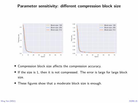
Parameter sensitivity: different compression block size

0 10 20 30 40 50 60 70Epoch

0.0

0.5

1.0

1.5

2.0

Trai

ning

Los

s

Block size: 128Block size: 256Block size: 512

0 10 20 30 40 50 60 70Epoch

0.00

0.25

0.50

0.75

1.00

1.25

1.50

1.75

2.00

Test

Los

s

Block size: 128Block size: 256Block size: 512

• Compression block size affects the compression accuracy.• If the size is 1, then it is not compressed. The error is large for large block

size.• These figures show that a moderate block size is enough.


Parameter sensitivity: different α and β

0 10 20 30 40 50 60 70Epoch

0.0

0.5

1.0

1.5

2.0

Trai

ning

Los

s

: 0.1: 0.2: 0.3

0 10 20 30 40 50 60 70Epoch

0.00

0.25

0.50

0.75

1.00

1.25

1.50

1.75

2.00

Test

Los

s

: 0.1: 0.2: 0.3

0 10 20 30 40 50 60 70Epoch

0.0

0.5

1.0

1.5

2.0

Trai

ning

Los

s

: 0.8: 0.9: 1.0

0 10 20 30 40 50 60 70Epoch

0.00

0.25

0.50

0.75

1.00

1.25

1.50

1.75

2.00

Test

Los

s

: 0.8: 0.9: 1.0

• α is the number used to track the gradient approximation. When there iscompression, α is smaller than 1.• β is the ratio in the update of model.• The performance is similar for the chosen α values.


Parameter sensitivity: different η

0 10 20 30 40 50 60 70Epoch

0.0

0.5

1.0

1.5

2.0

Trai

ning

Los

s

: 0.8: 0.9: 1.0

0 10 20 30 40 50 60 70Epoch

0.00

0.25

0.50

0.75

1.00

1.25

1.50

1.75

2.00

Test

Los

s

: 0.8: 0.9: 1.0

• η is the ratio in the error compensation.• It shows that η < 1 is preferred.


Per-iteration time cost comparison

0.0010 0.0015 0.0020 0.0025 0.0030 0.0035 0.0040 0.0045 0.0050Bandwidth (1s/Mbit)

0.0

0.5

1.0

1.5

2.0

2.5

Sec

onds

SGDQSGDDORE

• Simulated per-iteration time cost.• We assume that the same computational time for all worker nodes. The

latency is also the same.• The difference is in the bits to be transferred.• Since DORE can reduce the number of bits by 95%, the communication

time is reduced significantly, comparing to other algorithms.


Thank You!• Y. Li, X. Liu, J. Tang, and M. Yan, A Double Residual Compression

Algorithm for Efficient Distributed Learning, arXiv:1910.07561.


https://arxiv.org/abs/1910.07561

https://arxiv.org/abs/1910.07561

data compression in distributed learning

Documents