data analysis: preparing for your research data analysis using r · 2017-10-16 · preparing for...
TRANSCRIPT

Data analysis:
Preparing for your research data analysis using R

2 IT Learning Centre
Preparing for your research data analysis using R

3 IT Learning Centre
Preparing for your research data analysis using R
Revision Information
Version Date Author Changes made
2.0 Jan 2013 Esther Ng Created
2.1 October 2015 Steven Albury updates
2.2 October 2016 John Fresen Complete Revision
2.3 November 2016 John Fresen Complete Revision
2.4 February 2017 John Fresen Revision of content and slides
2.5 May 2017 John Fresen Complete Revision
Copyright
John Fresen make this document available under a Creative Commons license: Attribution, Non-Commercial, Share-Alike. Individual resources are subject to their own licensing conditions and all copyright of such resources is acknowledged.
Useful Websites Dr Mark Gardener R website http://www.gardenersown.co.uk/Education/Lectures/R/nonparam.htm#what_is_R R-bloggers Learn R https://www.r-bloggers.com/how-to-learn-r-2/ Quick-R website http://www.statmethods.net/index.html The Pirate’s Guide to R Dr Nathanial Phillips http://nathanieldphillips.com/thepiratesguidetor/ R-bloggers https://www.r-bloggers.com/ Germán Rodríguez Introducing R http://data.princeton.edu/R Michael Friendly’s website http://www.datavis.ca/ Alastair Sanderson http://www.sr.bham.ac.uk/~ajrs/R/index.html
Resources A strength of R is its help files. Use the internet – it has almost all the answers.
4 IT Learning Centre
Preparing for your research data analysis using R
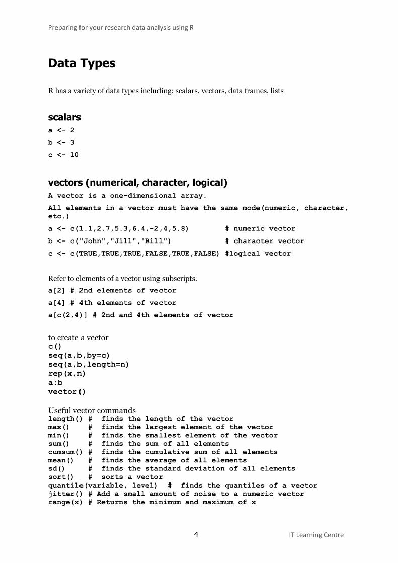
Data Types
R has a variety of data types including: scalars, vectors, data frames, lists
scalars
a <- 2
b <- 3
c <- 10
vectors (numerical, character, logical)
A vector is a one-dimensional array.
All elements in a vector must have the same mode(numeric, character,
etc.)
a <- c(1.1,2.7,5.3,6.4,-2,4,5.8) # numeric vector
b <- c("John","Jill","Bill") # character vector
c <- c(TRUE,TRUE,TRUE,FALSE,TRUE,FALSE) #logical vector
Refer to elements of a vector using subscripts.
a[2] # 2nd elements of vector
a[4] # 4th elements of vector
a[c(2,4)] # 2nd and 4th elements of vector
to create a vector c()
seq(a,b,by=c)
seq(a,b,length=n)
rep(x,n)
a:b
vector()
Useful vector commands length() # finds the length of the vector
max() # finds the largest element of the vector
min() # finds the smallest element of the vector
sum() # finds the sum of all elements
cumsum() # finds the cumulative sum of all elements
mean() # finds the average of all elements
sd() # finds the standard deviation of all elements
sort() # sorts a vector
quantile(variable, level) # finds the quantiles of a vector
jitter() # Add a small amount of noise to a numeric vector
range(x) # Returns the minimum and maximum of x
5 IT Learning Centre
Preparing for your research data analysis using R
rev(x) # List the elements of "x" in reverse order
matrices
A matrix is a two-dimensional array.
All columns in a matrix must have the same mode (numeric, character, etc.) and the same length.
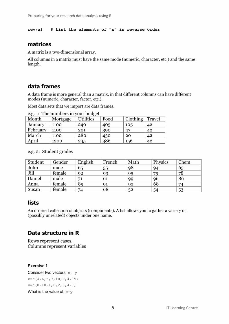
data frames
A data frame is more general than a matrix, in that different columns can have different modes (numeric, character, factor, etc.).
Most data sets that we import are data frames.
e.g. 1: The numbers in your budget Month Mortgage Utilities Food Clothing Travel January 1100 240 405 105 42 February 1100 201 390 47 42 March 1100 280 430 20 42 April 1200 245 386 156 42 e.g. 2: Student grades Student Gender English French Math Physics Chem John male 65 55 98 94 65 Jill female 92 93 95 75 78 Daniel male 71 61 99 96 86 Anna female 89 91 92 68 74 Susan female 74 68 52 54 53
lists
An ordered collection of objects (components). A list allows you to gather a variety of (possibly unrelated) objects under one name.
Data structure in R
Rows represent cases. Columns represent variables
Exercise 1
Consider two vectors, x, y
x=c(4,6,5,7,10,9,4,15)
y=c(0,10,1,8,2,3,4,1)
What is the value of: x*y

6 IT Learning Centre
Preparing for your research data analysis using R
Exercise 2
Consider two vectors, a, b
a=c(1,2,4,5,6)
b=c(3,2,4,1,9)
What is the value of: cbind(a,b)
Exercise 3
Consider two vectors, a, b
a=c(1,5,4,3,6)
b=c(3,5,2,1,9)
What is the value of: a<=b
What is the value of: which(a<=b)
Exercise 4
Consider two vectors, a, b
a=c(10,2,4,15)
b=c(3,12,4,11)
What is the value of: rbind(a,b)
What is the value of: cbind(a,b)
Exercise 5
If x=1:12
What is the value of: dim(x)
What is the value of: length(x)
Exercise 6
If a=12:5
What is the value of: is.numeric(a)
Exercise 7
Consider two vectors, x, y
x=12:4
y=c(0,1,2,0,1,2,0,1,2)
What is the value of: which(is.finite(x/y))
What is the value of: which(!is.finite(x/y))
Exercise 8
Consider two vectors, x, y
x=letters[1:10]
y=letters[15:24]
What is the value of: x<y
7 IT Learning Centre
Preparing for your research data analysis using R
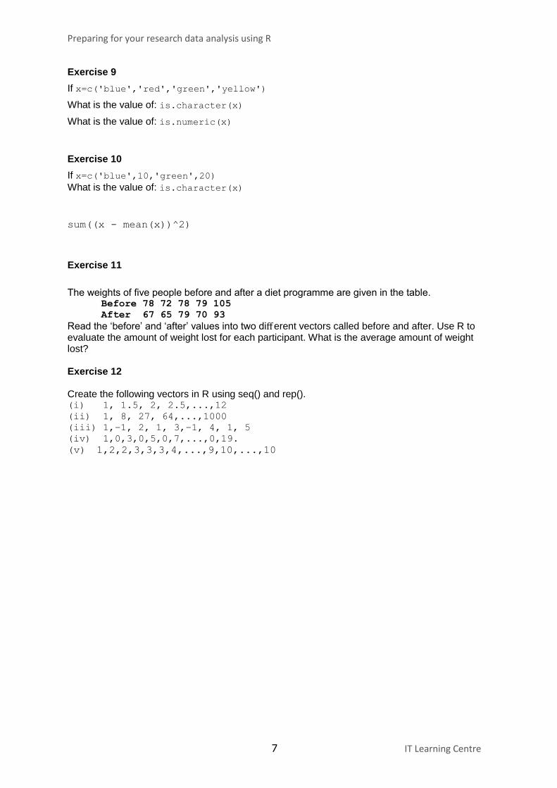
Exercise 9
If x=c('blue','red','green','yellow')
What is the value of: is.character(x)
What is the value of: is.numeric(x)
Exercise 10
If x=c('blue',10,'green',20)
What is the value of: is.character(x)
sum((x - mean(x))^2)
Exercise 11
The weights of five people before and after a diet programme are given in the table. Before 78 72 78 79 105
After 67 65 79 70 93
Read the ‘before’ and ‘after’ values into two different vectors called before and after. Use R to evaluate the amount of weight lost for each participant. What is the average amount of weight lost? Exercise 12 Create the following vectors in R using seq() and rep(). (i) 1, 1.5, 2, 2.5,...,12
(ii) 1, 8, 27, 64,...,1000
(iii) 1,−1, 2, 1, 3,−1, 4, 1, 5
(iv) 1,0,3,0,5,0,7,...,0,19.
(v) 1,2,2,3,3,3,4,...,9,10,...,10
8 IT Learning Centre
Preparing for your research data analysis using R
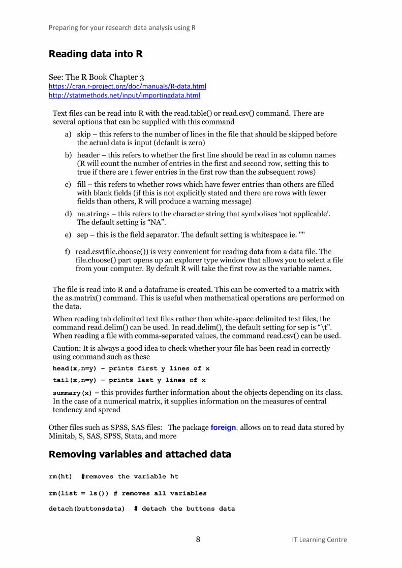
Reading data into R
See: The R Book Chapter 3 https://cran.r-project.org/doc/manuals/R-data.html http://statmethods.net/input/importingdata.html
Text files can be read into R with the read.table() or read.csv() command. There are several options that can be supplied with this command
a) skip – this refers to the number of lines in the file that should be skipped before the actual data is input (default is zero)
b) header – this refers to whether the first line should be read in as column names (R will count the number of entries in the first and second row, setting this to true if there are 1 fewer entries in the first row than the subsequent rows)
c) fill – this refers to whether rows which have fewer entries than others are filled with blank fields (if this is not explicitly stated and there are rows with fewer fields than others, R will produce a warning message)
d) na.strings – this refers to the character string that symbolises ‘not applicable’. The default setting is “NA”.
e) sep – this is the field separator. The default setting is whitespace ie. "" f) read.csv(file.choose()) is very convenient for reading data from a data file. The file.choose() part opens up an explorer type window that allows you to select a file from your computer. By default R will take the first row as the variable names.
The file is read into R and a dataframe is created. This can be converted to a matrix with the as.matrix() command. This is useful when mathematical operations are performed on the data.
When reading tab delimited text files rather than white-space delimited text files, the command read.delim() can be used. In read.delim(), the default setting for sep is “\t”. When reading a file with comma-separated values, the command read.csv() can be used.
Caution: It is always a good idea to check whether your file has been read in correctly using command such as these
head(x,n=y) – prints first y lines of x
tail(x,n=y) – prints last y lines of x
summary(x) – this provides further information about the objects depending on its class. In the case of a numerical matrix, it supplies information on the measures of central tendency and spread
Other files such as SPSS, SAS files: The package foreign, allows on to read data stored by Minitab, S, SAS, SPSS, Stata, and more
Removing variables and attached data
rm(ht) #removes the variable ht
rm(list = ls()) # removes all variables
detach(buttonsdata) # detach the buttons data

9 IT Learning Centre
Preparing for your research data analysis using R
Topics
1. Two sample tests
2. One-way ANOVA
3. Two-way ANOVA
4. Multiple linear Regression
5. Chi-squared tests
6. Logistic Regression
7. Kernel Regression
8. Other Regressions
9. Probability distributions
10. Control statements and loops
11. Writing your own functions
Example 0: Graphics
Example 0: Graphics
Graphics
Read the buttonsdata.csv. data.0 <- read.csv(file.choose())
attach(data.4)
Please open a word document into which you can develop your code and paste the results and graphics output from R. There are 2 different types of plotting commands – high level and low level. High level commands create a new plot on the graphics device, low level commands add information to an existing plot.
High level plotting commands
These always start a new plot, erasing anything already on the graphics device. Axes, labels and titles are created with the automatic default settings. We consider the following high level plotting commands:
• hist()
• barplot()
• boxplot()
• plot()
• qqplot() and qqline()
• pairs()
• par()
# par(mfrow=c(2,3)) partitions the graphics window into
# a matrix with 2 rows and 3 columns
We consider the following low level plotting commands that add to the existing plot:
• abline()
• lines()
• points()
• locator()
• text()
plot() command
The plot() function is the most commonly used graphical function in R. The type of plot that results depends on the arguments supplied.
If plot(x,y) is typed in, a scatterplot of y against x is produced if both are vectors.
If plot (x) is typed in and x is a vector, the values of x will be plotted against their index. If x is a matrix with 2 columns, the first column will be plotted against the second column.
Other formats include plot(x~y), plot(f,y) where f is a factor object and plot(~expr) etc. These are detailed in the help pages on plot.
Example 0: Graphics
To produce a scatterplot representing the relationship between height and weight, for the buttonsdata, we can use the following command
plot(ht,wt) or plot(wt~ht)
This gives a plot of all our data. But, we might want to do a number of things:
• add a title to "Plot of weight vs. height for buttons data"
• re-label the axes to "height (inches) " and "weight (pounds) " use xlab="height (in)" use ylab="weight (lbs)"
• control the limits of each axis: height between 50 and 90 - use xlim=c(50,90)
weight between 50 and 250 - use ylim=c(50,250)
• colour diabetics in red and non-diabetics in blue diab <- which(db==1) non.diab <- which(db==0)
• add grid lines abline(v=c(55,60,65,70,75,80))
abline(h=c(100,120,140,160,180,200))
and even much more • • •
plot(ht[diab],wt[diab], xlab="height(in)", ylab="weight(lbs)",
xlim=c(55,80), ylim=c(95,200), col="red",
main="Plot of weight vs. height for buttons data\n diabetes in
red; non-diabetes in blue")
points(ht[non.diab],wt[non.diab],col="blue")
abline(v=c(55,60,65,70,75,80))
abline(h=c(100,120,140,160,180,200))
hist() command Let’s put histograms of ht, wt and BMI into a 1 by 3 matrix of plots Frequency histograms: par(mfrow=c(1,3))
hist(ht,col="grey")
hist(wt,col="grey")
hist(bmi,col="grey")
Probability histograms: par(mfrow=c(1,3))
hist(ht,col="grey",prob=T)
hist(wt,col="grey",prob=T)
hist(bmi,col="grey",prob=T)
barplot() and table command
Let’s create tables for db and bp using the table() command and then plot barplots of the table, and put them in a 1 by 2 matric of plots: table(db)
table(bp)
par(mfrow=c(1,2))
barplot(table(db),col=c("lightblue","mistyrose"),
main="Barplot comparison of Normal vs. Diabetic",
Example 0: Graphics
names.arg = c("Normal","Diabetic"))
barplot(table(bp), col=c("lightblue","mistyrose"),
main="Barplot comparison of Normal vs. Hypertensive",
names.arg = c("Normal","Hypertensive"))
Tasks:
• use the ylim() function, inside the barplot command, to get the y-axis on both the
above graphs the same
• by dividing the table() by the number of observations, inside the barplot
command, convert the above barplots to probabilities (percentages)
boxplot() command Boxplots express the relationship between 2 variables, one continuous and one discrete. They represent a five point summary - the smallest observation (sample minimum), lower quartile (Q1), median (Q2), upper quartile (Q3), and largest observation (sample maximum). Let’s plot boxplots of ht against db, ht against bp, weight against db, wt against bp in a 1 by 4 matrix of plots. Here is the first boxplot:
boxplot(ht~db, col="grey")
Task
use help for boxplot to find out how to put names on the x-axis put appropriate main headings onto the plots
qqplot(), qqnorm() and qqline() commands a Q–Q plot ("Q" stands for quantile) is a probability plot, which is a graphical method for comparing two probability distributions by plotting their quantiles against each other. First, the set of intervals for the quantiles is chosen. A point (x, y) on the plot corresponds to one of the quantiles of the second distribution (y-coordinate) plotted against the same quantile of the first distribution (x-coordinate) If the two distributions being compared are similar, the points in the Q–Q plot will approximately lie on the line y = x. If the distributions are linearly related, the points in the Q–Q plot will approximately lie on a line, but not necessarily on the line y = x. The most common use of the qqplot is to check for normality. This is achieved a combination of the qqnorm() and qqline() which superimposes the line on which the plot would lie if it were normally distributed. Deviation from the line suggests deviation from normality. In reality no data are ever exactly normal, the normal distribution is at best a simple approximation.

Example 0: Graphics
Task:
Check ht, wt and bmi for normality using qqnorm() and qqline() by plotting three plots
on a 1 by 3 matrix of plots. Add suitable axes labels and titles. qqnorm(ht)
qqline(ht)
These many different plot functions are detailed in the document http://cran.r- project.org/doc/manuals/R-intro.pdf
Some other options for modifying the graph include
text() – adds text to the graph
legend() – adds a legend to the graph
abline() – adds a line in the format y=ax+b
polygon() – adds a polygon
A full list can be found in the ‘Introduction to R’ manual on the R website.

Two Sample Tests in R
Two Sample Tests Basically, the t-test compares two conditional distributions making the assumptions
• that both samples are random
• independent of each other
• come from normally distributed population with unknow but equal variances.
If we can’t assume equal variances, we can modify the test, and specify this in the formulation of the test. But this distorts our thinking a bit.
As a numeric example, consider the hypothetical weights (lb) of boxers and wrestlers below, posing the question: Assuming equal variances, do boxers and wrestlers come from populations with the same mean?
boxers: 175, 168, 168, 190, 156, 181, 182, 175, 174, 179 wrestlers: 185, 169, 173, 173, 188, 186, 175, 174, 179, 180
These data are stored in the file fighter_weights.csv
If we cannot assume normality, we use the non-parametric test called Wilcoxon-Mann-Whitney test; we will see this test in a future post.
Before proceeding with the t-test, we check the approximate normality using a Q-Q plot and evaluate the assumption of homoskedasticity (homogeneity of variances) of the two groups, using a Fisher’s F-test.
In R you can do this as follows:
Read the data data.1 <- read.csv(file.choose())
attach(data.1)
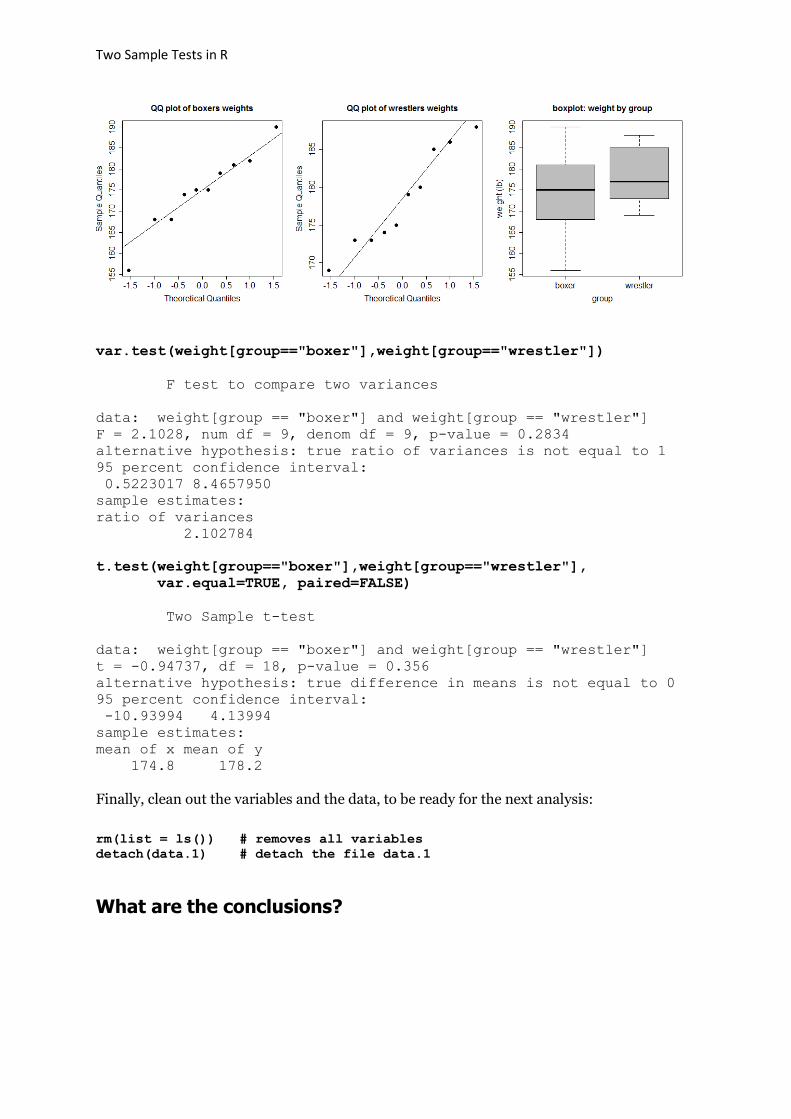
Plot the two data vectors using a Q-Q plots to check for approximate normality and using side-by-side boxplots to get an idea of the two conditional distributions.
par(mfrow=c(1,3))
qqnorm(salary[sex == "m"], pch=19, cex=1.5,
main= "QQ plot of male salaries", cex.main=1.5, cex.lab=1.5, cex.axis=1.5)
qqline(salary[sex == "m"])
qqnorm(salary[sex == "f"], pch=19, cex=1.5,
main= "QQ plot of female salaries", cex.main=1.5, cex.lab=1.5, cex.axis=1.5)
qqline(salary[sex == "f"])
boxplot(salary~sex, col="grey", main= "boxplot: salary by gender", xlab= "group", ylab= "weight (lb)", cex.main=1.5, cex.lab=1.5, cex.axis=1.5)
Two Sample Tests in R
var.test(weight[group=="boxer"],weight[group=="wrestler"])
F test to compare two variances
data: weight[group == "boxer"] and weight[group == "wrestler"]
F = 2.1028, num df = 9, denom df = 9, p-value = 0.2834
alternative hypothesis: true ratio of variances is not equal to 1
95 percent confidence interval:
0.5223017 8.4657950
sample estimates:
ratio of variances
2.102784
t.test(weight[group=="boxer"],weight[group=="wrestler"],
var.equal=TRUE, paired=FALSE)
Two Sample t-test
data: weight[group == "boxer"] and weight[group == "wrestler"]
t = -0.94737, df = 18, p-value = 0.356
alternative hypothesis: true difference in means is not equal to 0
95 percent confidence interval:
-10.93994 4.13994
sample estimates:
mean of x mean of y
174.8 178.2
Finally, clean out the variables and the data, to be ready for the next analysis:
rm(list = ls()) # removes all variables
detach(data.1) # detach the file data.1
What are the conclusions?
Practical 2: One way ANOVA
Practical 2: One way ANOVA chickwts The one-way ANOVA compares two or more conditional distributions making the assumptions
• that the samples are random
• independent of each other
• come from normally distributed population with unknow but equal variances.
It generalizes the two sample t-test to many samples.
As a numeric example, consider the chickwts data.
An experiment was conducted to measure and compare the effectiveness of various feed supplements on the growth rate of chickens.
Format: A data frame with 71 observations on the following 2 variables. weight: a numeric variable giving the chick weight. feed: a factor giving the feed type.
Details: Newly hatched chicks were randomly allocated into six groups, and each group was given a different feed supplement. Their weights in grams after six weeks are given along with feed types.
Source: Anonymous (1948) Biometrika, 35, 214.
Plan:
1. Read the data into R 2. Obtain Q-Q plots for each group 3. Plot side-by-side boxplots for each group 4. Check variance assumptions (using Bartlett’s test) 5. Perform ANOVA 6. Do multiple comparisons
data.2 <- read.csv(file.choose())
attach(data.2)
par(mfrow=c(1,6))
qqnorm(weight[feed == "horsebean"], pch=19, cex=1.5,
main= "QQ horsebean", cex.main=1.5, cex.lab=1.5, cex.axis=1.5)
qqline(weight[feed == "horsebean"])
qqnorm(weight[feed == "linseed"], pch=19, cex=1.5,
main= "QQ linseed", cex.main=1.5, cex.lab=1.5, cex.axis=1.5)
qqline(weight[feed == "linseed"])
qqnorm(weight[feed == "soybean"], pch=19, cex=1.5,
main= "QQ soybean", cex.main=1.5, cex.lab=1.5, cex.axis=1.5)
qqline(weight[feed == "soybean"])
qqnorm(weight[feed == "sunflower"], pch=19, cex=1.5,
main= "QQ sunflower", cex.main=1.5, cex.lab=1.5, cex.axis=1.5)
qqline(weight[feed == "sunflower"])
Practical 2: One way ANOVA
qqnorm(weight[feed == "meatmeal"], pch=19, cex=1.5,
main= "QQ meatmeal", cex.main=1.5, cex.lab=1.5, cex.axis=1.5)
qqline(weight[feed == "meatmeal"])
qqnorm(weight[feed == "casein"], pch=19, cex=1.5,
main= "QQ casein", cex.main=1.5, cex.lab=1.5, cex.axis=1.5)
qqline(weight[feed == "casein"])
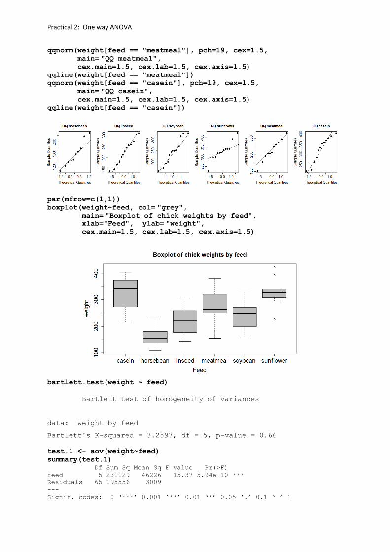
par(mfrow=c(1,1))
boxplot(weight~feed, col= "grey", main= "Boxplot of chick weights by feed", xlab="Feed", ylab= "weight", cex.main=1.5, cex.lab=1.5, cex.axis=1.5)
bartlett.test(weight ~ feed)
Bartlett test of homogeneity of variances
data: weight by feed
Bartlett's K-squared = 3.2597, df = 5, p-value = 0.66
test.1 <- aov(weight~feed)
summary(test.1)
Df Sum Sq Mean Sq F value Pr(>F)
feed 5 231129 46226 15.37 5.94e-10 ***
Residuals 65 195556 3009
---
Signif. codes: 0 ‘***’ 0.001 ‘**’ 0.01 ‘*’ 0.05 ‘.’ 0.1 ‘ ’ 1
Practical 2: One way ANOVA
Pairwise Comparisons – Bonferoni adjusted
pairwise.t.test(weight, feed, p.adjust="bonferroni")
Pairwise comparisons using t tests with pooled SD
data: weight and feed
casein horsebean linseed meatmeal soybean
horsebean 3.1e-08 - - - -
linseed 0.00022 0.22833 - - -
meatmeal 0.68350 0.00011 0.20218 - -
soybean 0.00998 0.00487 1.00000 1.00000 -
sunflower 1.00000 1.2e-08 9.3e-05 0.39653 0.00447
P value adjustment method: bonferroni
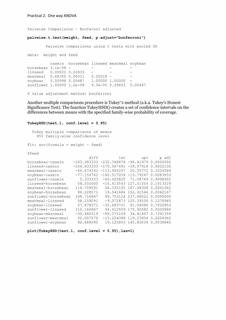
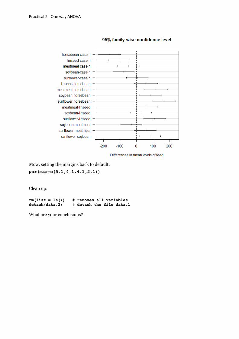
Another multiple comparisons procedure is Tukey‟s method (a.k.a. Tukey's Honest Significance Test). The function TukeyHSD() creates a set of confidence intervals on the differences between means with the specified family-wise probability of coverage.
TukeyHSD(test.1, conf.level = 0.95)
Tukey multiple comparisons of means
95% family-wise confidence level
Fit: aov(formula = weight ~ feed)
$feed
diff lwr upr p adj
horsebean-casein -163.383333 -232.346876 -94.41979 0.0000000
linseed-casein -104.833333 -170.587491 -39.07918 0.0002100
meatmeal-casein -46.674242 -113.906207 20.55772 0.3324584
soybean-casein -77.154762 -140.517054 -13.79247 0.0083653
sunflower-casein 5.333333 -60.420825 71.08749 0.9998902
linseed-horsebean 58.550000 -10.413543 127.51354 0.1413329
meatmeal-horsebean 116.709091 46.335105 187.08308 0.0001062
soybean-horsebean 86.228571 19.541684 152.91546 0.0042167
sunflower-horsebean 168.716667 99.753124 237.68021 0.0000000
meatmeal-linseed 58.159091 -9.072873 125.39106 0.1276965
soybean-linseed 27.678571 -35.683721 91.04086 0.7932853
sunflower-linseed 110.166667 44.412509 175.92082 0.0000884
soybean-meatmeal -30.480519 -95.375109 34.41407 0.7391356
sunflower-meatmeal 52.007576 -15.224388 119.23954 0.2206962
sunflower-soybean 82.488095 19.125803 145.85039 0.0038845
plot(TukeyHSD(test.1, conf.level = 0.95),las=1)
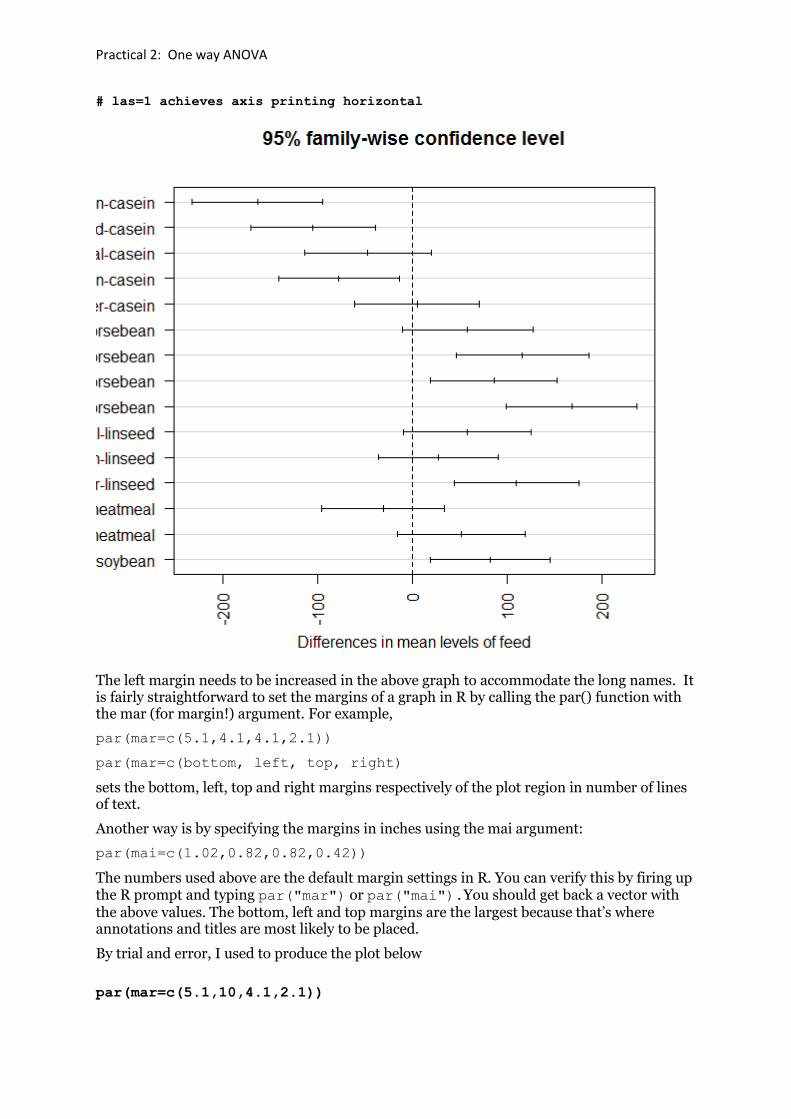
Practical 2: One way ANOVA
# las=1 achieves axis printing horizontal
The left margin needs to be increased in the above graph to accommodate the long names. It is fairly straightforward to set the margins of a graph in R by calling the par() function with the mar (for margin!) argument. For example,
par(mar=c(5.1,4.1,4.1,2.1))
par(mar=c(bottom, left, top, right)
sets the bottom, left, top and right margins respectively of the plot region in number of lines of text.
Another way is by specifying the margins in inches using the mai argument:
par(mai=c(1.02,0.82,0.82,0.42))
The numbers used above are the default margin settings in R. You can verify this by firing up the R prompt and typing par("mar") or par("mai").You should get back a vector with the above values. The bottom, left and top margins are the largest because that’s where annotations and titles are most likely to be placed.
By trial and error, I used to produce the plot below
par(mar=c(5.1,10,4.1,2.1))
Practical 2: One way ANOVA
Mow, setting the margins back to default:
par(mar=c(5.1,4.1,4.1,2.1))
Clean up:
rm(list = ls()) # removes all variables
detach(data.2) # detach the file data.1
What are your conclusions?
Example 3: Two-way ANOVA potato yield
Example 3: Two-way ANOVA potato yield Two-way ANOVA, like all ANOVAs, assumes that
• the observations are independent
• are normally distributed
• have equal standard deviations
The mean and spread of the conditional distributions are modelled under these assumptions. If any of these is in doubt, the ANOVA calculations are correspondingly in doubt.
Although some formal checks are possible via tests statistics, graphical representations are often the best check.
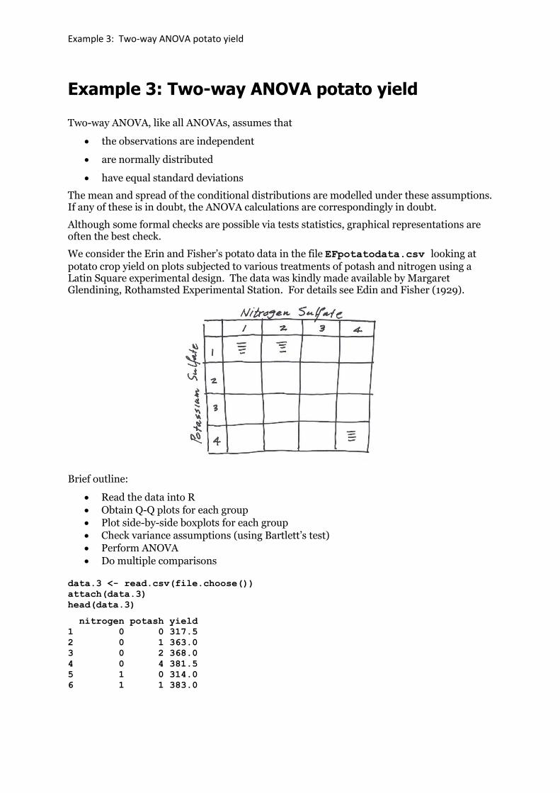
We consider the Erin and Fisher’s potato data in the file EFpotatodata.csv looking at
potato crop yield on plots subjected to various treatments of potash and nitrogen using a Latin Square experimental design. The data was kindly made available by Margaret Glendining, Rothamsted Experimental Station. For details see Edin and Fisher (1929).
Brief outline:
• Read the data into R
• Obtain Q-Q plots for each group
• Plot side-by-side boxplots for each group
• Check variance assumptions (using Bartlett’s test)
• Perform ANOVA
• Do multiple comparisons
data.3 <- read.csv(file.choose())
attach(data.3)
head(data.3)
nitrogen potash yield
1 0 0 317.5
2 0 1 363.0
3 0 2 368.0
4 0 4 381.5
5 1 0 314.0
6 1 1 383.0
Example 3: Two-way ANOVA potato yield
Means and summary statistics by group
library(Rmisc)
sum = summarySE(data.3,
measurevar="yield",
groupvars=c("nitrogen","potash"))
round(sum[,1:5],1)
nitrogen potash N yield sd
1 0 0 4 349.6 39.4
2 0 1 4 349.4 27.8
3 0 2 4 359.0 23.2
4 0 4 4 348.9 78.2
5 1 0 4 346.2 38.3
6 1 1 4 402.2 25.0
7 1 2 4 410.9 45.3
8 1 4 4 403.5 40.4
9 2 0 4 421.1 80.8
10 2 1 4 472.9 50.9
11 2 2 4 461.2 45.6
12 2 4 4 467.9 27.5
13 4 0 4 426.9 84.6
14 4 1 4 499.5 35.5
15 4 2 4 520.6 29.0
16 4 4 4 552.6 16.2
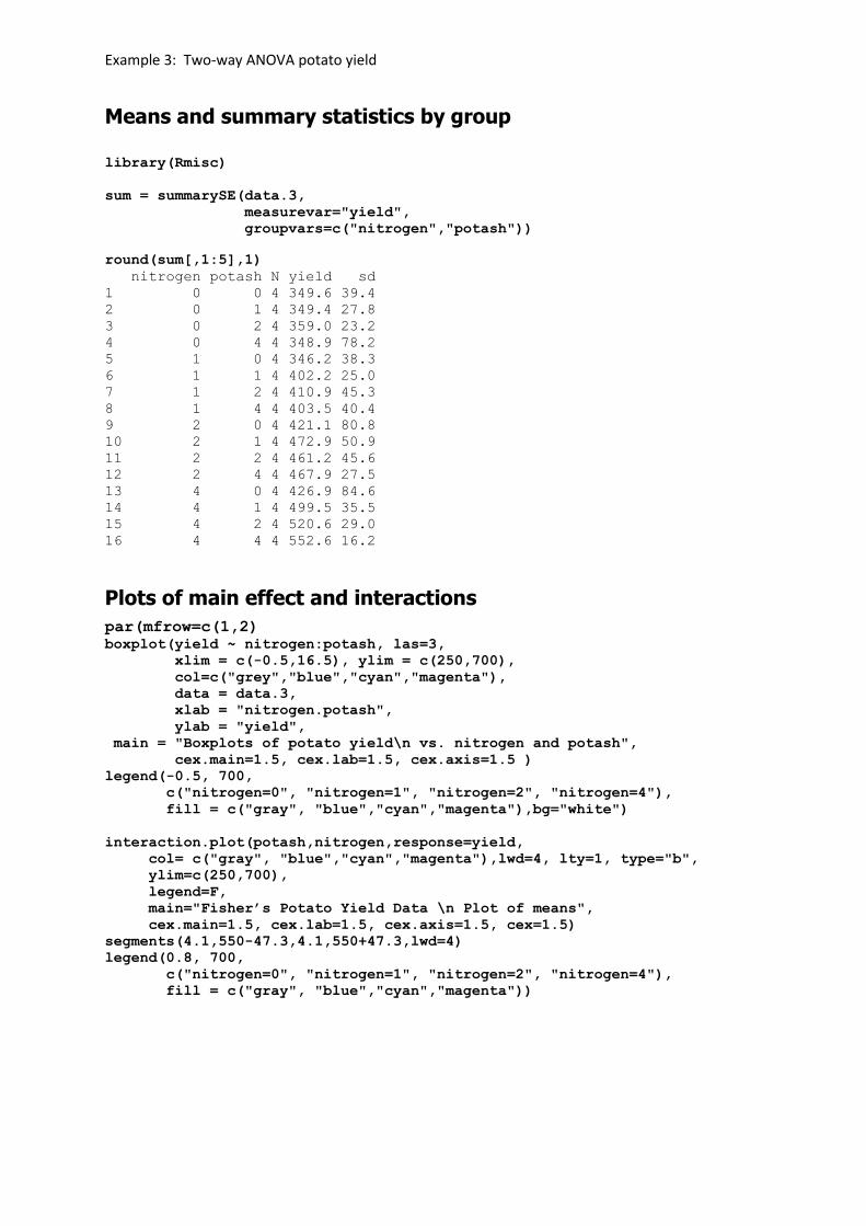
Plots of main effect and interactions
par(mfrow=c(1,2)
boxplot(yield ~ nitrogen:potash, las=3,
xlim = c(-0.5,16.5), ylim = c(250,700),
col=c("grey","blue","cyan","magenta"),
data = data.3,
xlab = "nitrogen.potash",
ylab = "yield",
main = "Boxplots of potato yield\n vs. nitrogen and potash",
cex.main=1.5, cex.lab=1.5, cex.axis=1.5 )
legend(-0.5, 700,
c("nitrogen=0", "nitrogen=1", "nitrogen=2", "nitrogen=4"),
fill = c("gray", "blue","cyan","magenta"),bg="white")
interaction.plot(potash,nitrogen,response=yield,
col= c("gray", "blue","cyan","magenta"),lwd=4, lty=1, type="b",
ylim=c(250,700),
legend=F,
main="Fisher’s Potato Yield Data \n Plot of means",
cex.main=1.5, cex.lab=1.5, cex.axis=1.5, cex=1.5)
segments(4.1,550-47.3,4.1,550+47.3,lwd=4)
legend(0.8, 700,
c("nitrogen=0", "nitrogen=1", "nitrogen=2", "nitrogen=4"),
fill = c("gray", "blue","cyan","magenta"))
Example 3: Two-way ANOVA potato yield
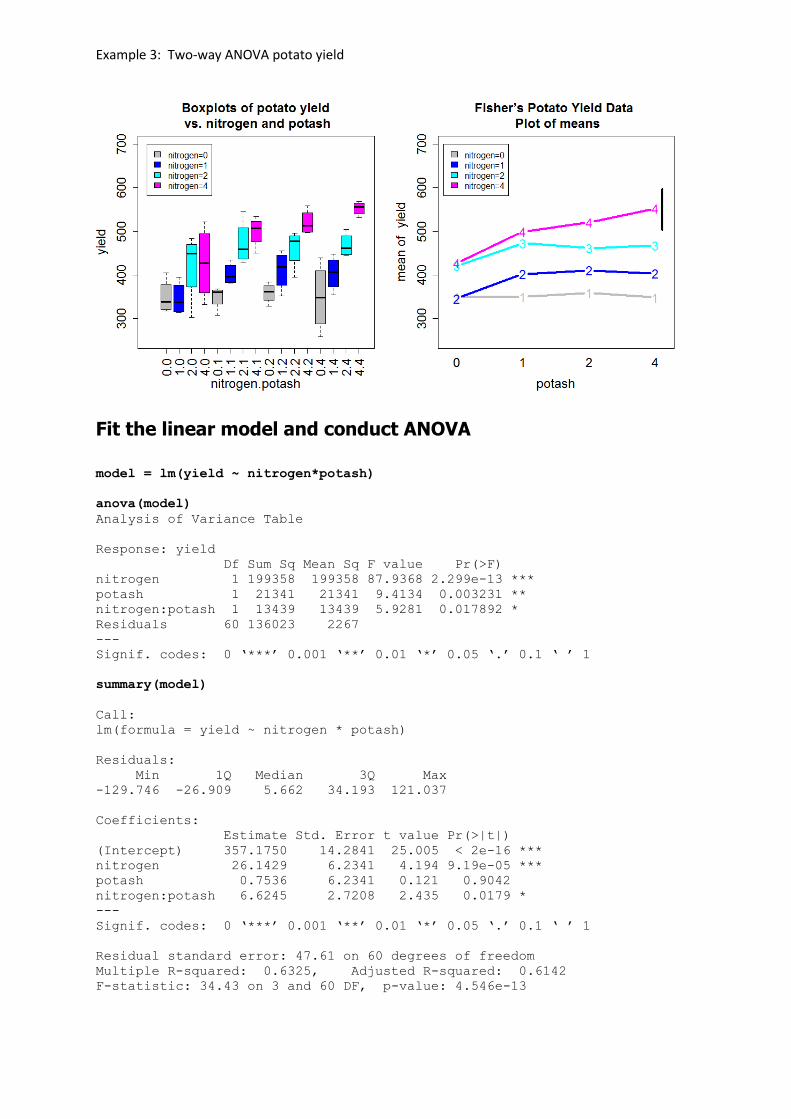
Fit the linear model and conduct ANOVA
model = lm(yield ~ nitrogen*potash)
anova(model)
Analysis of Variance Table
Response: yield
Df Sum Sq Mean Sq F value Pr(>F)
nitrogen 1 199358 199358 87.9368 2.299e-13 ***
potash 1 21341 21341 9.4134 0.003231 **
nitrogen:potash 1 13439 13439 5.9281 0.017892 *
Residuals 60 136023 2267
---
Signif. codes: 0 ‘***’ 0.001 ‘**’ 0.01 ‘*’ 0.05 ‘.’ 0.1 ‘ ’ 1
summary(model)
Call:
lm(formula = yield ~ nitrogen * potash)
Residuals:
Min 1Q Median 3Q Max
-129.746 -26.909 5.662 34.193 121.037
Coefficients:
Estimate Std. Error t value Pr(>|t|)
(Intercept) 357.1750 14.2841 25.005 < 2e-16 ***
nitrogen 26.1429 6.2341 4.194 9.19e-05 ***
potash 0.7536 6.2341 0.121 0.9042
nitrogen:potash 6.6245 2.7208 2.435 0.0179 *
---
Signif. codes: 0 ‘***’ 0.001 ‘**’ 0.01 ‘*’ 0.05 ‘.’ 0.1 ‘ ’ 1
Residual standard error: 47.61 on 60 degrees of freedom
Multiple R-squared: 0.6325, Adjusted R-squared: 0.6142
F-statistic: 34.43 on 3 and 60 DF, p-value: 4.546e-13
Example 3: Two-way ANOVA potato yield
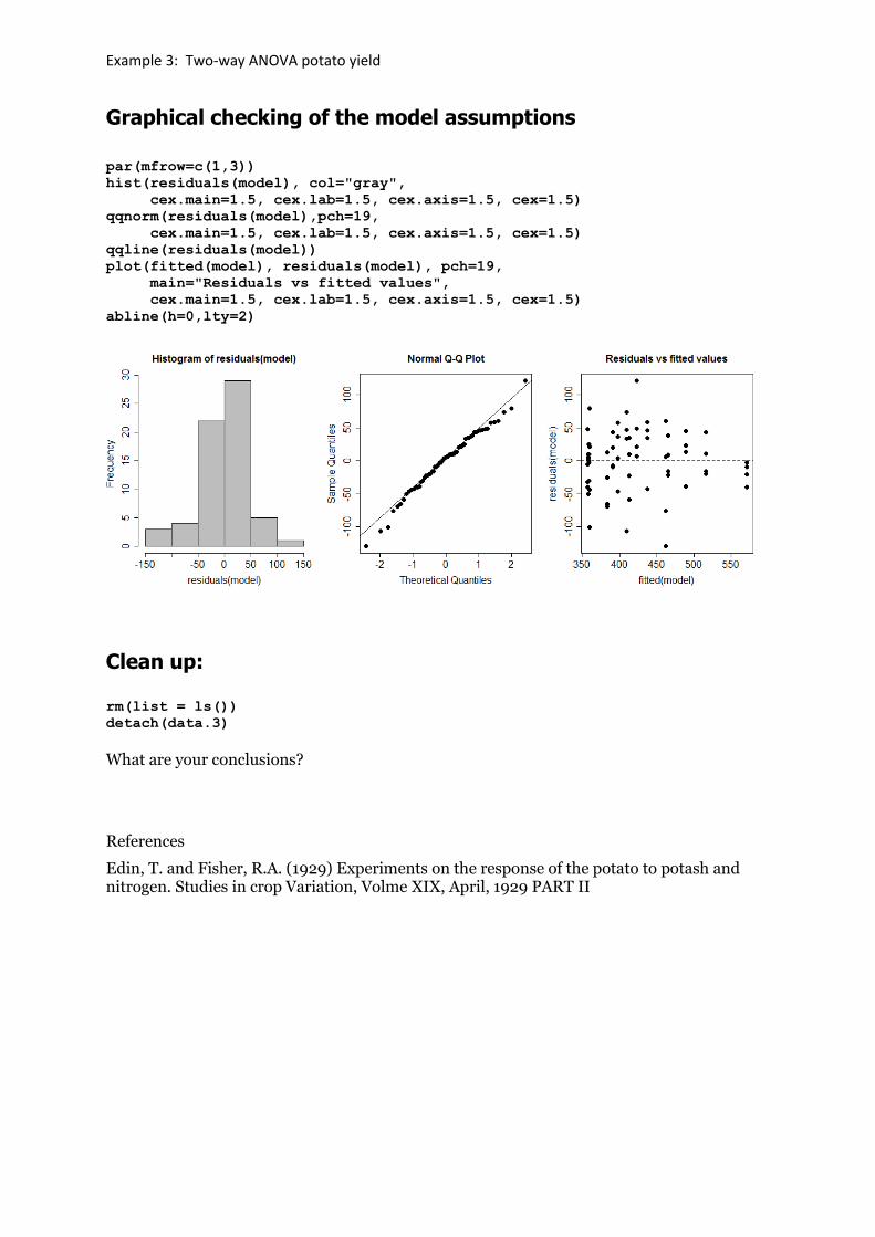
Graphical checking of the model assumptions
par(mfrow=c(1,3))
hist(residuals(model), col="gray",
cex.main=1.5, cex.lab=1.5, cex.axis=1.5, cex=1.5)
qqnorm(residuals(model),pch=19,
cex.main=1.5, cex.lab=1.5, cex.axis=1.5, cex=1.5)
qqline(residuals(model))
plot(fitted(model), residuals(model), pch=19,
main="Residuals vs fitted values",
cex.main=1.5, cex.lab=1.5, cex.axis=1.5, cex=1.5)
abline(h=0,lty=2)
Clean up:
rm(list = ls())
detach(data.3)
What are your conclusions?
References
Edin, T. and Fisher, R.A. (1929) Experiments on the response of the potato to potash and nitrogen. Studies in crop Variation, Volme XIX, April, 1929 PART II
Example 4: Multiple Linear Regression
Example 4: Multiple Linear Regression Regression assumes that
• the observations are independent
• are normally distributed
• means lie on a straight line
• have equal standard deviations
The mean and spread of the conditional distributions are modelled under these assumptions. If any of these is in doubt, the regression calculations are correspondingly in doubt.
Although some formal checks are possible via tests statistics, graphical representations are often the best check.
Problem and Data
The data given in the appendix were collected on 31 cherry trees and represent the
• diameter (in inches) at a height of 4.5 feet from the ground
• height (in feet) of the tree, and the
• volume of usable wood (in cubic feet) that was cut from the harvested tree
The objective was to develop a model to predict the volume of usable wood from the measurements of the diameter and height of the tree so as to be able to estimate the economic value of wood yield for a plantation of cherry trees.
Model Building Considerations
To guide our model building, we might model a tree as either a cylinder or a cone, as a first approximation. To this end, recall that the volume of a cylinder of diameter d and height h is
4/2hdv
and that the volume of a cone of base diameter d and height h is
12/2hdv .
Taking logs of these formulae transforms the multiplicative model into an additive model. Thus, we have
)4ln()ln()ln(2)ln()ln( hdv
for a cylinder and
)12ln()ln()ln(2)ln()ln( hdv
Example 4: Multiple Linear Regression
for a cone. These suggest that it may be useful to transform the data to logs before fitting a
linear regression model. Denote the transformed variables by )ln(vlv , )ln(dld ,
)ln(hlh .
Brief outline
Perform an analysis that will lead to a regression model for predicting the average volume of useful wood that can be cut from a tree of given diameter and height. You might consider, inter-alia, the following points in your analysis but do not be restricted to this list.
Consider the univariate marginal distributions, the matrix of scatter plots, and comment on the correlation of the predictor variables. Are the transformed variables normally distributed?
1. Fit the regression model, construct the ANOVA table, the summary of estimated coefficients, assess and interpret the regression.
2. Perform a graphical analysis of the residuals to assess if the assumptions on the error terms are reasonable.
3. Are both predictor variables necessary? If not, which is the better variable to retain? Fit the appropriate model and assess and interpret it.
4. How accurate is the prediction equation?
5. Can you make useful simple recommendations about estimating the volume of usable wood from measurements of diameter and height?
Cherry Tree Analysis
Step 1: Read and attach data
data.4 <- read.csv(file.choose())
attach(data.4)
head(data.4)
d h v
1 8.3 70 10.3
2 8.6 65 10.3
3 8.8 63 10.2
4 10.5 72 16.4
5 10.7 81 18.8
6 10.8 83 19.7
Step 2: compute the log-transformed data
ld <- log(d)
lh <- log(h)
lv <- log(v)
Example 4: Multiple Linear Regression
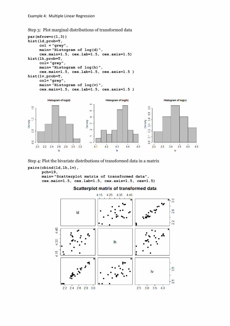
Step 3: Plot marginal distributions of transformed data
par(mfrow=c(1,3))
hist(ld,prob=T,
col = "grey", main= "Histogram of log(d)", cex.main=1.5, cex.lab=1.5, cex.axis=1.5)
hist(lh,prob=T,
col= "grey", main= "Histogram of log(h)", cex.main=1.5, cex.lab=1.5, cex.axis=1.5 )
hist(lv,prob=T,
col= "grey", main= "Histogram of log(v)", cex.main=1.5, cex.lab=1.5, cex.axis=1.5 )
Step 4: Plot the bivariate distributions of transformed data in a matrix
pairs(cbind(ld,lh,lv),
pch=19,
main= "Scatterplot matrix of transformed data", cex.main=1.5, cex.lab=1.5, cex.axis=1.5, cex=1.5)
Example 4: Multiple Linear Regression
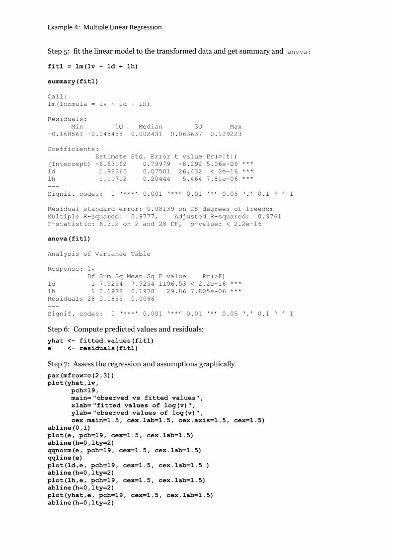
Step 5: fit the linear model to the transformed data and get summary and anova:
fit1 = lm(lv ~ ld + lh)
summary(fit1)
Call:
lm(formula = lv ~ ld + lh)
Residuals:
Min 1Q Median 3Q Max
-0.168561 -0.048488 0.002431 0.063637 0.129223
Coefficients:
Estimate Std. Error t value Pr(>|t|)
(Intercept) -6.63162 0.79979 -8.292 5.06e-09 ***
ld 1.98265 0.07501 26.432 < 2e-16 ***
lh 1.11712 0.20444 5.464 7.81e-06 ***
---
Signif. codes: 0 ‘***’ 0.001 ‘**’ 0.01 ‘*’ 0.05 ‘.’ 0.1 ‘ ’ 1
Residual standard error: 0.08139 on 28 degrees of freedom
Multiple R-squared: 0.9777, Adjusted R-squared: 0.9761
F-statistic: 613.2 on 2 and 28 DF, p-value: < 2.2e-16
anova(fit1)
Analysis of Variance Table
Response: lv
Df Sum Sq Mean Sq F value Pr(>F)
ld 1 7.9254 7.9254 1196.53 < 2.2e-16 ***
lh 1 0.1978 0.1978 29.86 7.805e-06 ***
Residuals 28 0.1855 0.0066
---
Signif. codes: 0 ‘***’ 0.001 ‘**’ 0.01 ‘*’ 0.05 ‘.’ 0.1 ‘ ’ 1
Step 6: Compute predicted values and residuals:
yhat <- fitted.values(fit1)
e <- residuals(fit1)
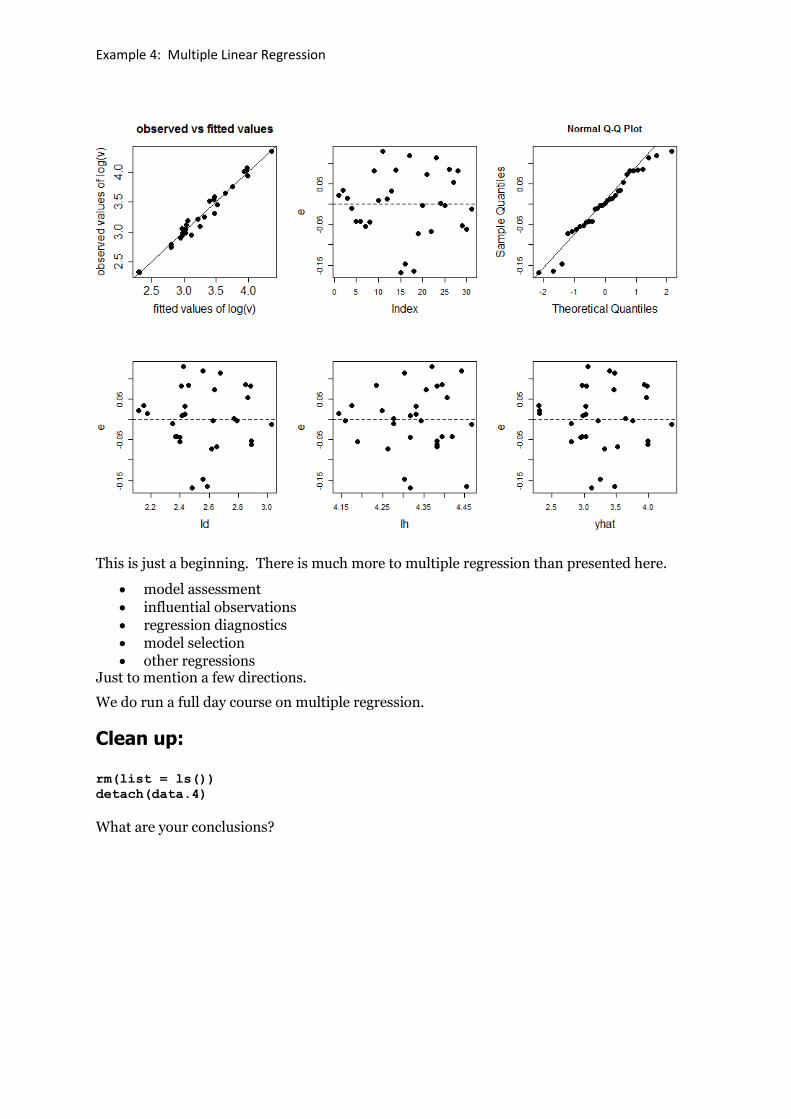
Step 7: Assess the regression and assumptions graphically
par(mfrow=c(2,3))
plot(yhat,lv,
pch=19,
main= "observed vs fitted values", xlab= "fitted values of log(v)", ylab= "observed values of log(v)", cex.main=1.5, cex.lab=1.5, cex.axis=1.5, cex=1.5)
abline(0,1)
plot(e, pch=19, cex=1.5, cex.lab=1.5)
abline(h=0,lty=2)
qqnorm(e, pch=19, cex=1.5, cex.lab=1.5)
qqline(e)
plot(ld,e, pch=19, cex=1.5, cex.lab=1.5 )
abline(h=0,lty=2)
plot(lh,e, pch=19, cex=1.5, cex.lab=1.5)
abline(h=0,lty=2)
plot(yhat,e, pch=19, cex=1.5, cex.lab=1.5)
abline(h=0,lty=2)
Example 4: Multiple Linear Regression
This is just a beginning. There is much more to multiple regression than presented here.
• model assessment
• influential observations
• regression diagnostics
• model selection
• other regressions Just to mention a few directions.
We do run a full day course on multiple regression.
Clean up:
rm(list = ls())
detach(data.4)
What are your conclusions?
Example 5: Chi-squared tests
Example 5: Chi-squared tests Chi-squared tests are usually used to compare two or more probability distributions, and usually to the discrete conditional distributions in a two-way table.
Example : Comparing two surveys – Chi-squared test
(Comparing two discrete probability distributions)
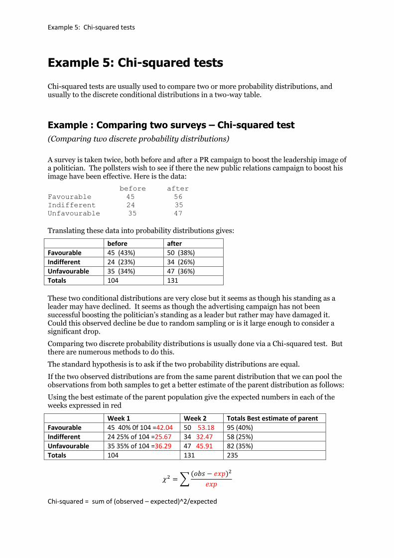
A survey is taken twice, both before and after a PR campaign to boost the leadership image of a politician. The pollsters wish to see if there the new public relations campaign to boost his image have been effective. Here is the data:
before after
Favourable 45 56
Indifferent 24 35
Unfavourable 35 47
Translating these data into probability distributions gives:
before after
Favourable 45 (43%) 50 (38%)
Indifferent 24 (23%) 34 (26%)
Unfavourable 35 (34%) 47 (36%)
Totals 104 131
These two conditional distributions are very close but it seems as though his standing as a leader may have declined. It seems as though the advertising campaign has not been successful boosting the politician’s standing as a leader but rather may have damaged it. Could this observed decline be due to random sampling or is it large enough to consider a significant drop.
Comparing two discrete probability distributions is usually done via a Chi-squared test. But there are numerous methods to do this.
The standard hypothesis is to ask if the two probability distributions are equal.
If the two observed distributions are from the same parent distribution that we can pool the observations from both samples to get a better estimate of the parent distribution as follows:
Using the best estimate of the parent population give the expected numbers in each of the weeks expressed in red
Week 1 Week 2 Totals Best estimate of parent
Favourable 45 40% 0f 104 =42.04 50 53.18 95 (40%)
Indifferent 24 25% of 104 =25.67 34 32.47 58 (25%)
Unfavourable 35 35% of 104 =36.29 47 45.91 82 (35%)
Totals 104 131 235
𝜒2 =∑(𝑜𝑏𝑠 − 𝑒𝑥𝑝)2
𝑒𝑥𝑝
Chi-squared = sum of (observed – expected)^2/expected
Example 5: Chi-squared tests
before after
Results of Survey Before vs After
0.0
0.1
0.2
0.3
0.4
0.5
Fav
Ind
Unfav
Fav
Ind
Unfav
= (45-42.04)^2/42.04 + (24-25.67)^2/25.67 + . . . + (47-45.91)^2/45.91 This follows a Chi-squared distribution with 2 degrees of freedom.
How do we do this in R?
Enter data via keyboard x <- matrix(c(45,24,35,50,34,47),3,2)
chisq.test(x)
Pearson's Chi-squared test output
data: x
X-squared = 0.64984, df = 2, p-value = 0.7226
Conclusion: The large p-value suggests that this is a non-significant
difference between the two probability distributions.
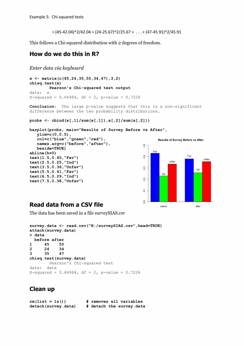
probs <- cbind(x[,1]/sum(x[,1]),x[,2]/sum(x[,2]))
barplot(probs, main="Results of Survey Before vs After",
ylim=c(0,0.5),
col=c("blue","green","red"),
names.arg=c("before","after"),
beside=TRUE)
abline(h=0)
text(1.5,0.45,"Fav")
text(2.5,0.25,"Ind")
text(3.5,0.36,"Unfav")
text(5.5,0.41,"Fav")
text(6.5,0.29,"Ind")
text(7.5,0.38,"Unfav")
Read data from a CSV file
The data has been saved in a file surveySIAS.csv
survey.data <- read.csv("E:/surveySIAS.csv",head=TRUE)
attach(survey.data)
> data
before after
1 45 50
2 24 34
3 35 47
chisq.test(survey.data)
Pearson's Chi-squared test
data: data
X-squared = 0.64984, df = 2, p-value = 0.7226
Clean up
rm(list = ls()) # removes all variables
detach(survey.data) # detach the survey.data
Example 6: Logistic Regression UWC data
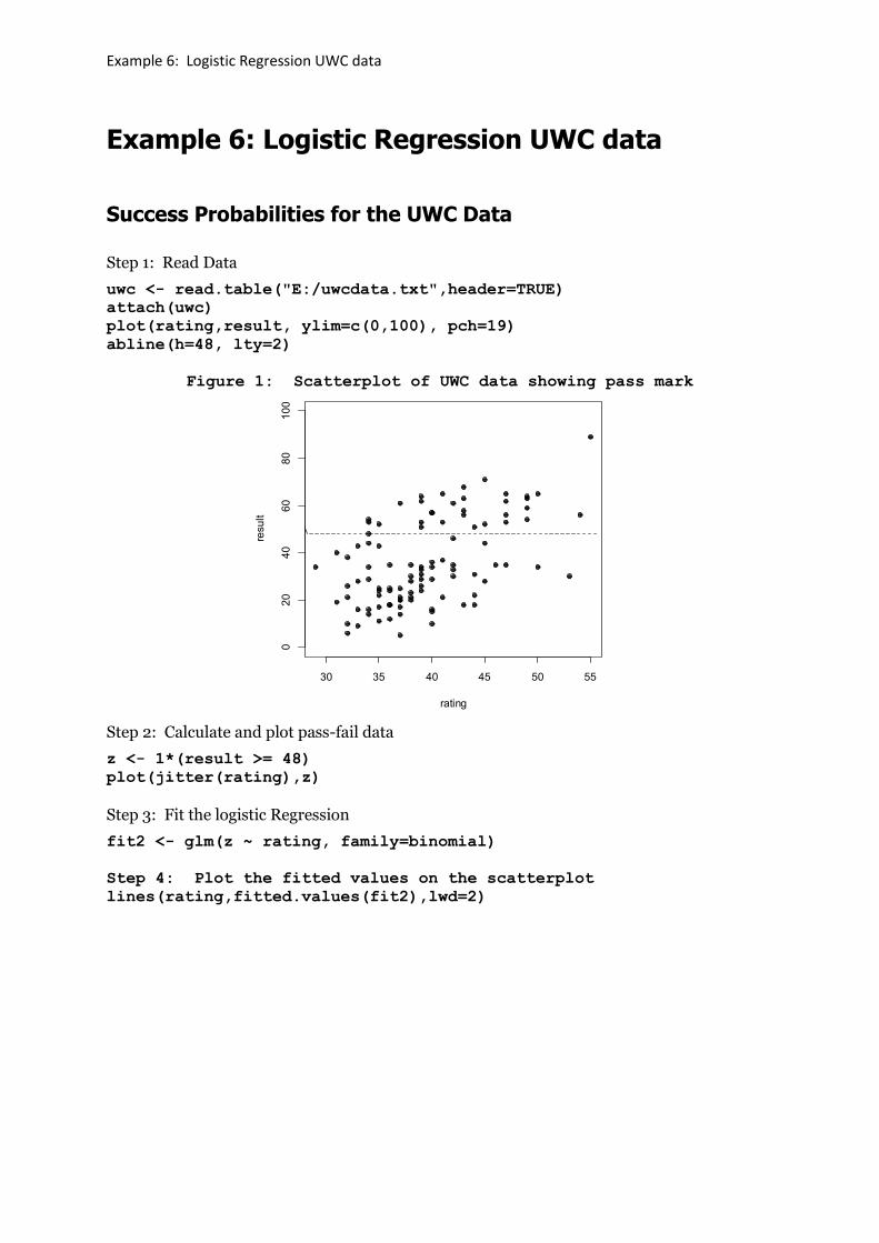
Example 6: Logistic Regression UWC data
Success Probabilities for the UWC Data
Step 1: Read Data
uwc <- read.table("E:/uwcdata.txt",header=TRUE)
attach(uwc)
plot(rating,result, ylim=c(0,100), pch=19)
abline(h=48, lty=2)
Figure 1: Scatterplot of UWC data showing pass mark
Step 2: Calculate and plot pass-fail data
z <- 1*(result >= 48)
plot(jitter(rating),z)
Step 3: Fit the logistic Regression
fit2 <- glm(z ~ rating, family=binomial)
Step 4: Plot the fitted values on the scatterplot
lines(rating,fitted.values(fit2),lwd=2)
30 35 40 45 50 55
020
40
60
80
100
rating
result
Example 6: Logistic Regression UWC data
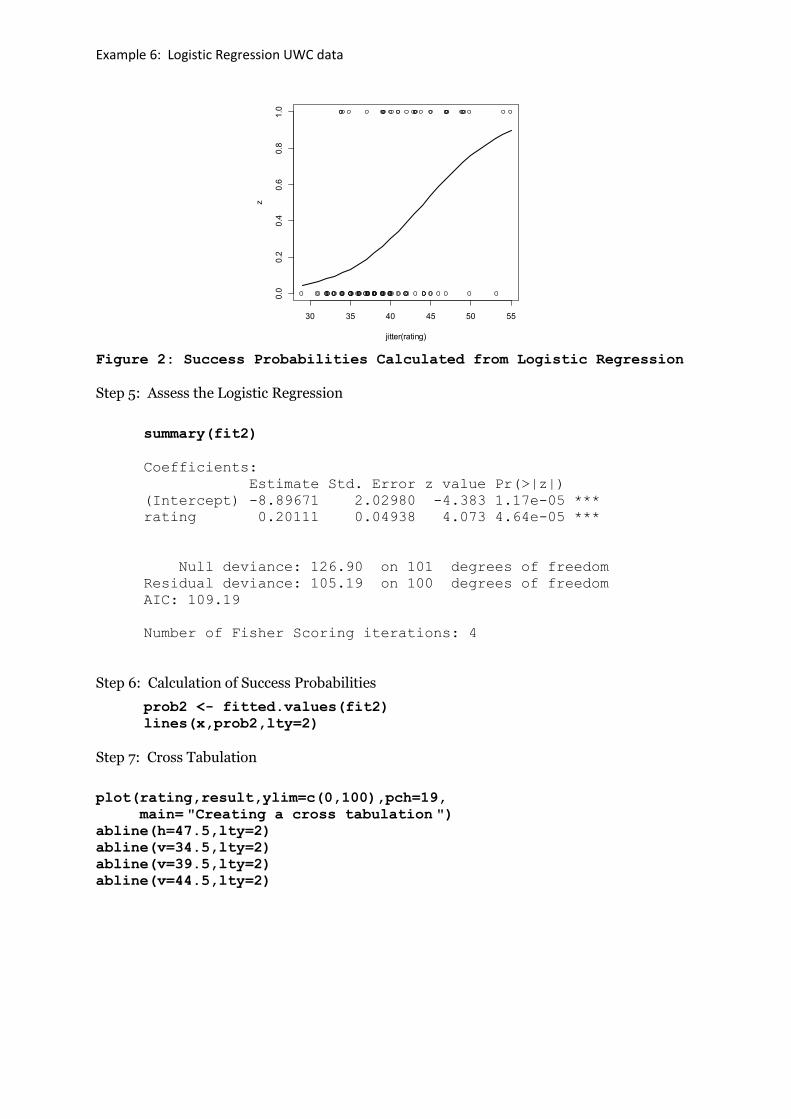
Figure 2: Success Probabilities Calculated from Logistic Regression
Step 5: Assess the Logistic Regression
summary(fit2)
Coefficients:
Estimate Std. Error z value Pr(>|z|)
(Intercept) -8.89671 2.02980 -4.383 1.17e-05 ***
rating 0.20111 0.04938 4.073 4.64e-05 ***
Null deviance: 126.90 on 101 degrees of freedom
Residual deviance: 105.19 on 100 degrees of freedom
AIC: 109.19
Number of Fisher Scoring iterations: 4
Step 6: Calculation of Success Probabilities
prob2 <- fitted.values(fit2)
lines(x,prob2,lty=2)
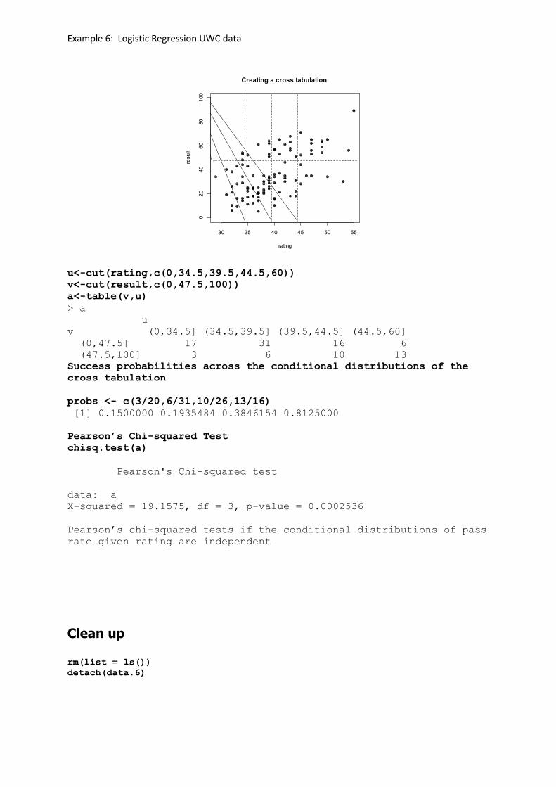
Step 7: Cross Tabulation
plot(rating,result,ylim=c(0,100),pch=19,
main= "Creating a cross tabulation ") abline(h=47.5,lty=2)
abline(v=34.5,lty=2)
abline(v=39.5,lty=2)
abline(v=44.5,lty=2)
30 35 40 45 50 55
0.0
0.2
0.4
0.6
0.8
1.0
jitter(rating)
z
Example 6: Logistic Regression UWC data
u<-cut(rating,c(0,34.5,39.5,44.5,60))
v<-cut(result,c(0,47.5,100))
a<-table(v,u)
> a
u
v (0,34.5] (34.5,39.5] (39.5,44.5] (44.5,60]
(0,47.5] 17 31 16 6
(47.5,100] 3 6 10 13
Success probabilities across the conditional distributions of the
cross tabulation
probs <- c(3/20,6/31,10/26,13/16)
[1] 0.1500000 0.1935484 0.3846154 0.8125000
Pearson’s Chi-squared Test
chisq.test(a)
Pearson's Chi-squared test
data: a
X-squared = 19.1575, df = 3, p-value = 0.0002536
Pearson’s chi-squared tests if the conditional distributions of pass
rate given rating are independent
Clean up
rm(list = ls())
detach(data.6)
30 35 40 45 50 55
020
40
60
80
100
Creating a cross tabulation
rating
result
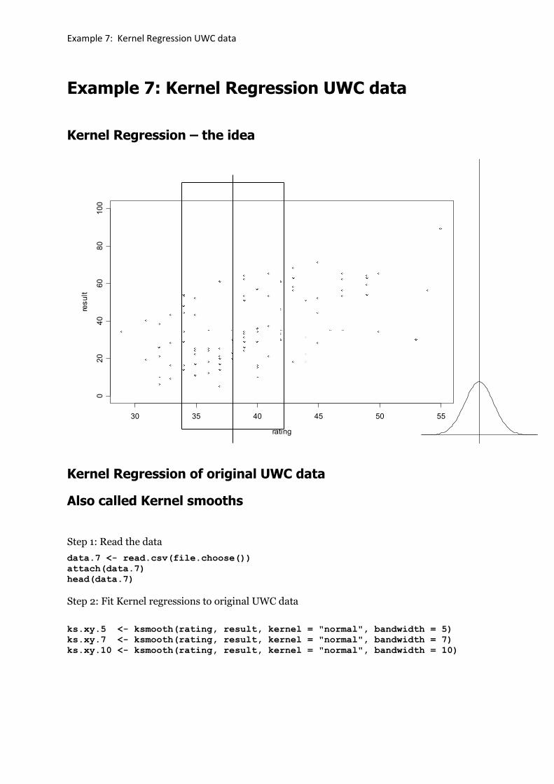
Example 7: Kernel Regression UWC data
Example 7: Kernel Regression UWC data
Kernel Regression – the idea
Kernel Regression of original UWC data
Also called Kernel smooths
Step 1: Read the data
data.7 <- read.csv(file.choose())
attach(data.7)
head(data.7)
Step 2: Fit Kernel regressions to original UWC data
ks.xy.5 <- ksmooth(rating, result, kernel = "normal", bandwidth = 5)
ks.xy.7 <- ksmooth(rating, result, kernel = "normal", bandwidth = 7)
ks.xy.10 <- ksmooth(rating, result, kernel = "normal", bandwidth = 10)
rating
result
30 35 40 45 50 55
020
40
60
80
100
-4 -2 0 2 4
0.0
0.5
1.0
1.5
2.0
x
y
Example 7: Kernel Regression UWC data
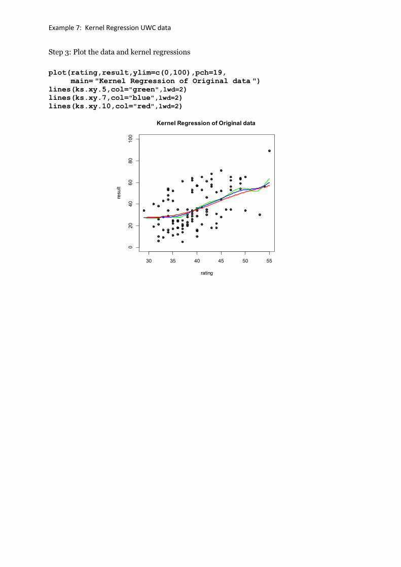
Step 3: Plot the data and kernel regressions
plot(rating,result,ylim=c(0,100),pch=19,
main= "Kernel Regression of Original data ") lines(ks.xy.5,col="green",lwd=2)
lines(ks.xy.7,col="blue",lwd=2)
lines(ks.xy.10,col="red",lwd=2)
30 35 40 45 50 55
020
40
60
80
100
Kernel Regression of Original data
rating
result
Example 7: Kernel Regression UWC data
Kernel Regression of UWC pass-fail data
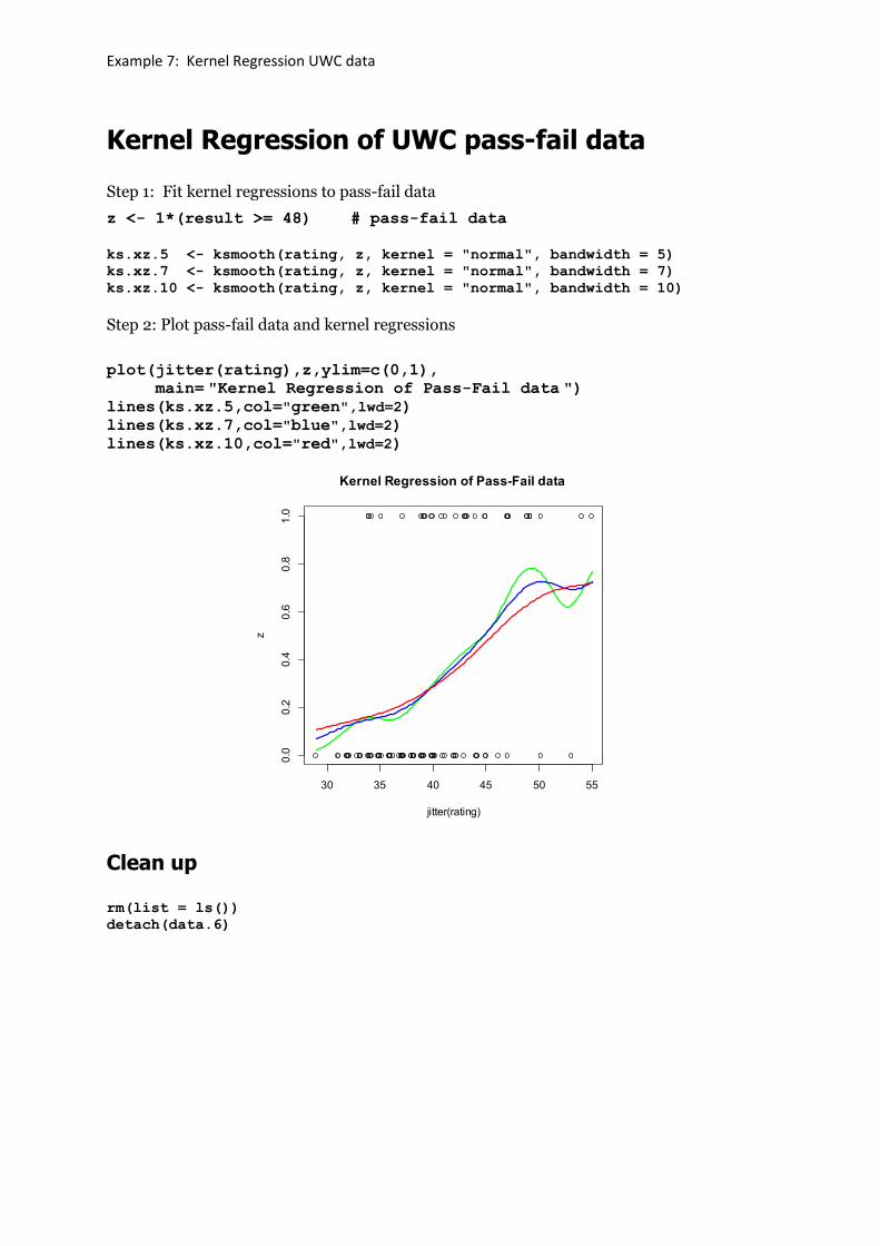
Step 1: Fit kernel regressions to pass-fail data
z <- 1*(result >= 48) # pass-fail data
ks.xz.5 <- ksmooth(rating, z, kernel = "normal", bandwidth = 5)
ks.xz.7 <- ksmooth(rating, z, kernel = "normal", bandwidth = 7)
ks.xz.10 <- ksmooth(rating, z, kernel = "normal", bandwidth = 10)
Step 2: Plot pass-fail data and kernel regressions
plot(jitter(rating),z,ylim=c(0,1),
main= "Kernel Regression of Pass-Fail data ") lines(ks.xz.5,col="green",lwd=2)
lines(ks.xz.7,col="blue",lwd=2)
lines(ks.xz.10,col="red",lwd=2)
Clean up
rm(list = ls())
detach(data.6)
30 35 40 45 50 55
0.0
0.2
0.4
0.6
0.8
1.0
Kernel Regression of Pass-Fail data
jitter(rating)
z
Example 8: Other Regressions UWC data
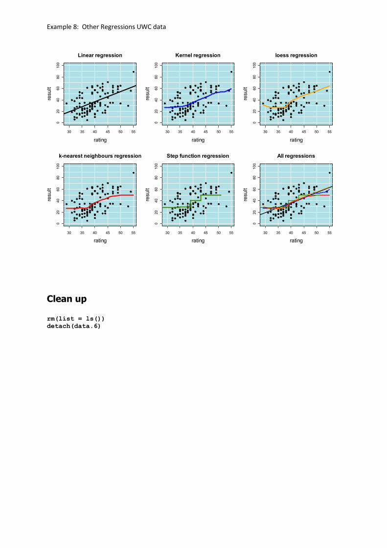
Example 8: Other Regressions UWC data
Other Regressions
Once one realises that regression is modelling the mean of conditional distributions many possibilities open up. Here are a few alternatives – but there are many, many more.
Our conclusions, for any analysis, depend in part on the assumptions and algorithm chosen. If various methods corroborate, that reinforces our belief in the conclusions.
lm, ksmooth, loess, kknn, step regressions
library(kknn)
fit.lm <- lm(result~rating)
fit.ksm.7 <- ksmooth(rating,result,kernel="normal",bandwidth=7)
fit.loess <- loess(result~rating)
yhat.loess <- fitted.values(fit.loess)
fit.kknn.40 <- kknn(formula=result~rating, k=40, distance=2,
train=uwc,test=NULL)
yhat.kknn.40 <- fitted.values(fit.kknn.40)
## fit a sep function - steps at quartiles of rating x = c(35,39,43)
## meansin each region y = c(a,b,c,d)
x <- quantile(rating,probs=c(0.25,0.5,0.75))
a <- mean(result[rating<=35])
b <- mean(result[rating>35 & rating<=39])
c <- mean(result[rating>39 & rating<=43])
d <- mean(result[rating>43])
y = c(a,b,c,d)
step.fun <- stepfun(x,y)
plot(rating,result,ylim=c(0,100))
lines(step.fun)
## Plot individual regressions on a 2 by 3 matrix of scatterplots
par(mfrow=c(2,3))
# linear regression
plot(rating,result,ylim=c(0,100),
main="Linear regression",
cex.main = 1.5,cex.lab = 1.5)
rect(par("usr")[1], par("usr")[3], par("usr")[2], par("usr")[4], col =
"powderblue")
abline(h=seq(0,100,by=10),col="white")
abline(v=seq(30,55,by=5),col="white")
points(rating,result,pch=19)
abline(fit.lm, lwd=3)
Example 8: Other Regressions UWC data
## kernel regression
plot(rating,result,ylim=c(0,100),
main="Kernel regression",
cex.main = 1.5,cex.lab = 1.5)
rect(par("usr")[1], par("usr")[3], par("usr")[2], par("usr")[4], col =
"powderblue")
abline(h=seq(0,100,by=10),col="white")
abline(v=seq(30,55,by=5),col="white")
points(rating,result,pch=19)
lines(fit.ksm.7,col="blue",lwd=3)
## loess regression
plot(rating,result,ylim=c(0,100),
main="loess regression",
cex.main = 1.5,cex.lab = 1.5)
rect(par("usr")[1], par("usr")[3], par("usr")[2], par("usr")[4], col =
"powderblue")
abline(h=seq(0,100,by=10),col="white")
abline(v=seq(30,55,by=5),col="white")
points(rating,result,pch=19)
lines(rating,yhat.loess,col="orange",lwd=3)
# KNN regression k-nearest neighbours
plot(rating,result,ylim=c(0,100),
main="k-nearest neighbours regression",
cex.main = 1.5,cex.lab = 1.5)
rect(par("usr")[1], par("usr")[3], par("usr")[2], par("usr")[4], col =
"powderblue")
abline(h=seq(0,100,by=10),col="white")
abline(v=seq(30,55,by=5),col="white")
points(rating,result,pch=19)
lines(rating,yhat.kknn.40, col="red",lwd=3)
## Step function regression
plot(rating,result,ylim=c(0,100),
main="Step function regression",
cex.main = 1.5,cex.lab = 1.5)
rect(par("usr")[1], par("usr")[3], par("usr")[2], par("usr")[4], col =
"powderblue")
abline(h=seq(0,100,by=10),col="white")
abline(v=seq(30,55,by=5),col="white")
points(rating,result,pch=19)
lines(step.fun,col="chartreuse4",lwd=3)
## add all fitted regressions: lm, ksmooth, loess, kknn, step
plot(rating,result,ylim=c(0,100),
main="All regressions",
cex.main = 1.5,cex.lab = 1.5)
rect(par("usr")[1], par("usr")[3], par("usr")[2], par("usr")[4], col =
"powderblue")
abline(h=seq(0,100,by=10),col="white")
abline(v=seq(30,55,by=5),col="white")
points(rating,result,pch=19)
abline(fit.lm, lwd=2)
lines(fit.ksm.7,col="blue",lwd=2)
lines(rating,yhat.loess,col="orange",lwd=2)
lines(rating,yhat.kknn.40, col="red",lwd=2)
lines(step.fun,col="chartreuse4",lwd=2)
Example 8: Other Regressions UWC data
Clean up
rm(list = ls())
detach(data.6)
30 35 40 45 50 55
020
40
60
80
100
Linear regression
rating
result
30 35 40 45 50 55
020
40
60
80
100
Kernel regression
rating
result
30 35 40 45 50 55
020
40
60
80
100
loess regression
rating
result
30 35 40 45 50 55
020
40
60
80
100
k-nearest neighbours regression
rating
result
30 35 40 45 50 55
020
40
60
80
100
Step function regression
rating
result
30 35 40 45 50 55
020
40
60
80
100
All regressions
ratingresult
Example 9: Probability distributions
Example 9: Probability distributions
See: http://cran.r-project.org/doc/manuals/R-intro.pdf (page 33)
R has a set of built-in functions related to probability
distributions. These functions can evaluate the
- probability density function (prefix the name with ‘d’)
- cumulative distribution function (prefix the name with ‘p’)
- quantile function (prefix the name with ‘q’)
- simulate from the distribution (prefix the name with ‘r’)
where the name refers to a set of R names eg. ‘norm’ (normal), ‘unif’ (uniform), ‘binom’ (binomial), ‘chisq’ (chi square), ‘hyper’ (hypergeometric) etc.
The full list can be found in the official R manual accessible here
Let’s generate a random sample of 1000 observations from a normal distribution with a mean of 5 and standard deviation of 2, and store the data in a vector “r.vals” (short for random values).
r.vals <- rnorm(1000, mean = 5, sd = 2)
(look up help for rnorm)
Task: Compute the summary and standard deviation of vals in a 1 by 2 matrix of plots:
• plot a probability histogram of r.vals – colour it grey
• generate a vector x of length 100 from the min(r.vals) to max(r.vals)
• compute a vector y equal to the density of the normal distribution with mean and sd
of r.vals
• superimpose the graph of x and y on the probability histogram of r.vals
• plot a qqnorm and superimpose a qqline of the data in r.vals
Example 10: Control statements and loops
Example 10: Control statements and loops See http://cran.r- project.org/doc/manuals/R-intro.pdf page 40 http://statmethods.net/management/controlstructures.html https://www.datacamp.com/community/tutorials/tutorial-on-loops-in-r#gs.uVzoMAk
If/Else and Ifelse
if (condition) expr_1 else expr_2
Example y <- 1
if(y>2) x<-3 else x <-4
x
[1] 4
Example z<-1
y<-1
if(y<2&&z<2) x<-3 else x <-4
x
[1] 3
Loops
This can be achieved with ‘for’ or ‘while’. The syntax is as follows… for (i in n:m){expr}
where n is the first value and m is the last value of i for which the expression within curly brackets should be evaluated
Example
my_results <- vector() # this creates an empty vector to store results
my_matrix <- matrix(c(1,2,3, 7,8,9), nrow = 2, ncol=3, byrow=TRUE)
my_matrix # this generates a matrix for testing purposes
my_matrix
[,1] [,2] [,3]
[1,] 1 2 3
[2,] 7 8 9
Example 10: Control statements and loops
for(i in 1:3){ #this loops through the numbers 1 to 3
+ mean(my_matrix[,i])-> my_results[i] # mean of each column in matrix
+ print(i)}
# this prints the counter so that we know which column we are up to
[1]
1
[1]
2
[1]
3
my_results
[1] 4 5 6
Exercise Loops and If/Else statements
In this exercise, we will explore loops and if/else statements in R
Task 1
Loops
Step 1
The dataset ‘airquality’ contains daily airquality measurements in New York in 1973. It is a dataframe with observation of 6 variables – mean ozone in parts perbillion, solar radiation, wind in miles perhour, temperature in degrees fahrenhait, month and day of month. View the first few lines of the dataset with the command head().
Step 2
For each day, we would like to create a hypothetical ‘wind- temperature’ score calculated by
2*Wind + temperature of that day – temperature of the next day
Write a loop to create this score for each day and store it in a vector. It is not necessary to calculate this value for the last day in the dataset. You should end up with a vector the length of the number of rows in the data frame minus one.
Hint – Let the loop variable i be the row-number
Task 2
If else statements
Step 1
For each day, we would like to create a conditional score based on temperature and solar radiation. If the solar radiation is higher than 150 units and the temperature is higher than 60 degrees fahrenhait, the score should be 1. If not, it should be 0. Write an ifelse statement to calculate this score for the all days in the dataset. You should end up with a vector of zeros and ones. The vector should be the same length as the number of rows in the dataset.
Example 11: Writing your own functions
Example 11: Writing your own functions http://cran.r- project.org/doc/manuals/R-intro.pdf page 42 When you need to perform a repeated function in R, a function can be written to perform this. The syntax to write a function is
my_function <- functionx(x){
y <- commands(x)
return(y)
}
Taking the example in the ‘loops’ exercise
The dataset in question is ‘airquality’ data(airquality)
attach(airquality)
For each day, we would like to create a conditional score based on temperature and solar radiation. If the solar radiation is higher than 150 units and the temperature is higher than 60 degrees fahrenhait, the score should be 1. If not, it should be 0. Write an ifelse statement to calculate this score for the all days in the dataset. You should end up with a vector of zeros and ones. The vector should be the same length as the number of rows in the dataset.
Instead of writing a loop, we can write a function and apply it to the matrix. The argument to the function would be row of the matrix
The function would be written as follows
calc_score <- function(x){
ifelse(x[2]>150|x[4]>60,1,0) -> y
return(y)
}
The function can then be applied to the matrix as follows
result <- apply(airquality, 1, calc_score)
Example 11: Writing your own functions
Exercise: Write a function to compute a Confidence Interval for a Correlation Coefficient (two sided)
let 𝑟 be a computed correlation coefficient based on 𝑛 observations. Write a function to use Fisher’s z-transformation to compute a confidence interval, with confidence coefficient 𝑝 (usually 𝑝 = 0.95) for 𝑟. The steps are given below: Step 1: transform 𝑟 to z: 𝑧 = 0.5 ∗ (ln(1 + 𝑟) − ln(1 − 𝑟)) Step 2: compute the quantile of the 𝑡 distribution, with 𝑛 − 2 degrees of freedom for the required confidence coefficient 𝑝 (usually 𝑝 = 0.95): 𝑞 = 𝑞𝑡(0.5 + 𝑝/2, 𝑛 − 2) Step 3: compute lower and upper confidence limits for z
𝑙𝑐𝑙. 𝑧 = 𝑧 − 𝑞/√𝑛 − 3
𝑢𝑐𝑙. 𝑧 = 𝑧 + 𝑞/√𝑛 − 3 Step 4: transform these lower and upper confidence limits back onto the 𝑟 scale: 𝑙𝑐𝑙. 𝑟 = exp(2 ∗ 𝑙𝑐𝑙. 𝑧 − 1) /exp(2 ∗ 𝑙𝑐𝑙. 𝑧 + 1) 𝑢𝑐𝑙. 𝑟 = exp(2 ∗ 𝑢𝑐𝑙. 𝑧 − 1) /exp(2 ∗ 𝑢𝑐𝑙. 𝑧 + 1) Try out you function using 𝑟 = 0.8, 𝑛 = 20, 𝑝 = 0.95 (lcl=0.529, ucl=0.923) 𝑟 = 0.8, 𝑛 = 100, 𝑝 = 0.95 (lcl=0.715, ucl= 0.862)
Solution: ci.corr <- function(r,n,p) {
z <- 0.5*(log(1+r) - log(1-r))
q <- qt(0.5+p/2,n-2)
lcl.z <- z - q/sqrt(n-3)
ucl.z <- z + q/sqrt(n-3)
lcl.r <- (exp(2*lcl.z)-1)/(exp(2*lcl.z)+1)
ucl.r <- (exp(2*ucl.z)-1)/(exp(2*ucl.z)+1)
result <- c(lcl.r,ucl.r)
return(result)
}

Practical 1 Two sample comparison of starting salaries
Practical 1: Comparison of starting salaries Consider the starting salary data, contained in the file startingsalaries.csv, giving
the starting salaries for both males and females at a bank in 1979.
The research hypothesis is that female salaries are less than male starting salaries
The null hypothesis is that male and female salaries are equal.
These data are stored in the file startingsalaries.csv
1. Read the data into R
2. Provide Q-Q plots and side-by-side boxplots of the starting salaries for males and females
3. Test the assumption of equal variances
4. Test the assumption of equal means
5. What are your conclusions?

Practical 1 Two sample comparison of starting salaries
Practical 1: Comparison of starting salaries Consider the starting salary data, contained in the file startingsalaries.csv, giving
the starting salaries for both males and females at a bank in 1979.
1. Read the data into R
2. Provide Q-Q plots and side-by-side boxplots of the starting salaries for males and females
3. Test the assumption of equal variances
4. Test the assumption of equal means
5. What are your conclusions?
Possible solutions:
data.2 <- read.csv(file.choose())
attach(data.2)
head(data.2)
salary sex
1 3900 f
2 4020 f
3 4290 f
4 4380 f
5 4380 f
6 4380 f
par(mfrow=c(1,3))
qqnorm(salary[sex == "m"], pch=19, cex=1.5,
main= "QQ plot of male salaries", cex.main=1.5, cex.lab=1.5, cex.axis=1.5)
qqline(salary[sex == "m"])
qqnorm(salary[sex == "f"], pch=19, cex=1.5,
main= "QQ plot of female salaries", cex.main=1.5, cex.lab=1.5, cex.axis=1.5)
qqline(salary[sex == "f"])
boxplot(salary~sex, col="grey", main= "boxplot: salary by sex", xlab= "sex", ylab= "salary", cex.main=1.5, cex.lab=1.5, cex.axis=1.5)
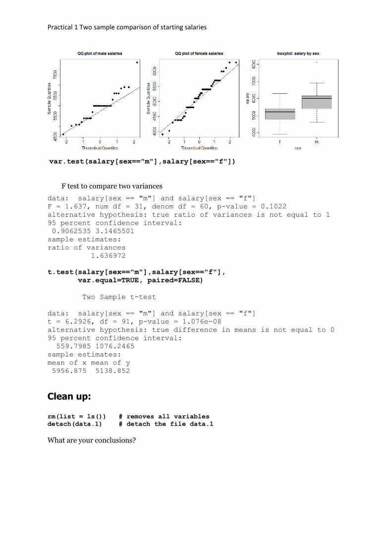
Practical 1 Two sample comparison of starting salaries
var.test(salary[sex=="m"],salary[sex=="f"])
F test to compare two variances
data: salary[sex == "m"] and salary[sex == "f"]
F = 1.637, num df = 31, denom df = 60, p-value = 0.1022
alternative hypothesis: true ratio of variances is not equal to 1
95 percent confidence interval:
0.9062535 3.1465501
sample estimates:
ratio of variances
1.636972
t.test(salary[sex=="m"],salary[sex=="f"],
var.equal=TRUE, paired=FALSE)
Two Sample t-test
data: salary[sex == "m"] and salary[sex == "f"]
t = 6.2926, df = 91, p-value = 1.076e-08
alternative hypothesis: true difference in means is not equal to 0
95 percent confidence interval:
559.7985 1076.2465
sample estimates:
mean of x mean of y
5956.875 5138.852
Clean up:
rm(list = ls()) # removes all variables
detach(data.1) # detach the file data.1
What are your conclusions?

Practical 1 Two sample comparison of starting salaries

Practical 2: One way ANOVA
Practical 2: One way ANOVA excavation data
Excavation Depth and Archaeology
Four different excavation sites at an archeological area in New Mexico gave the following depths (cm) for significant archaeological discoveries.
The data are stored in excavation.csv
X1 = depths at Site I
X2 = depths at Site II
X3 = depths at Site III
X4 = depths at Site IV
Reference: Mimbres Mogollon Archaeology by Woosley and McIntyre, Univ. of New
Mexico Press
1. Read the data into R 2. Obtain Q-Q plots for each group 3. Plot side-by-side boxplots for each group 4. Check variance assumptions (using Bartlett’s test) 5. Perform ANOVA 6. Do multiple comparisons

Practical 2: One way ANOVA
Practical 2: One way ANOVA excavation data Excavation Depth and Archaeology
Four different excavation sites at an archeological area in New Mexico gave the following depths (cm) for significant archaeological discoveries.
X1 = depths at Site I
X2 = depths at Site II
X3 = depths at Site III
X4 = depths at Site IV
Reference: Mimbres Mogollon Archaeology by Woosley and McIntyre, Univ. of New
Mexico Press
1. Read the data into R 2. Obtain Q-Q plots for each group 3. Plot side-by-side boxplots for each group 4. Check variance assumptions (using Bartlett’s test) 5. Perform ANOVA 6. Do multiple comparisons
data.2 <- read.csv(file.choose())
attach(data.2)
Declare site as a factor
site <- as.factor(site)
par(mfrow=c(1,4))
qqnorm(depth[site == 1], pch=19, cex=1.5,
main= "QQ Site 1", cex.main=1.5, cex.lab=1.5, cex.axis=1.5)
qqline(depth[site == 1])
qqnorm(depth[site == 2], pch=19, cex=1.5,
main= "QQ Site 2", cex.main=1.5, cex.lab=1.5, cex.axis=1.5)
qqline(depth[site == 2])
qqnorm(depth[site == 3], pch=19, cex=1.5,
main= "QQ Site 3", cex.main=1.5, cex.lab=1.5, cex.axis=1.5)
qqline(depth[site == 3])
qqnorm(depth[site == 4], pch=19, cex=1.5,
main= "QQ Site 4", cex.main=1.5, cex.lab=1.5, cex.axis=1.5)
qqline(depth[site == 4])
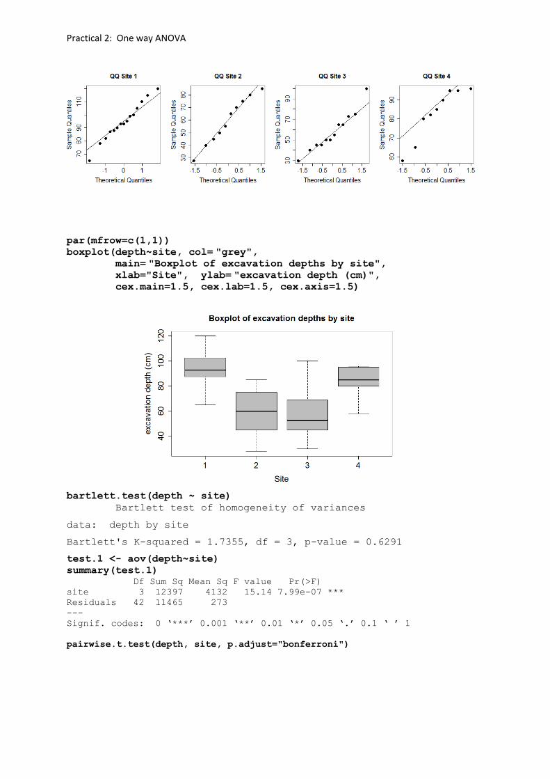
Practical 2: One way ANOVA
par(mfrow=c(1,1))
boxplot(depth~site, col= "grey", main= "Boxplot of excavation depths by site", xlab="Site", ylab= "excavation depth (cm)", cex.main=1.5, cex.lab=1.5, cex.axis=1.5)
bartlett.test(depth ~ site)
Bartlett test of homogeneity of variances
data: depth by site
Bartlett's K-squared = 1.7355, df = 3, p-value = 0.6291
test.1 <- aov(depth~site)
summary(test.1)
Df Sum Sq Mean Sq F value Pr(>F)
site 3 12397 4132 15.14 7.99e-07 ***
Residuals 42 11465 273
---
Signif. codes: 0 ‘***’ 0.001 ‘**’ 0.01 ‘*’ 0.05 ‘.’ 0.1 ‘ ’ 1
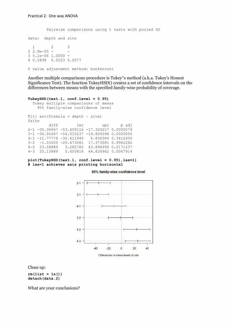
pairwise.t.test(depth, site, p.adjust="bonferroni")
Practical 2: One way ANOVA
Pairwise comparisons using t tests with pooled SD
data: depth and site
1 2 3
2 2.9e-05 - -
3 5.1e-06 1.0000 -
4 0.5898 0.0203 0.0077
P value adjustment method: bonferroni
Another multiple comparisons procedure is Tukey‟s method (a.k.a. Tukey's Honest Significance Test). The function TukeyHSD() creates a set of confidence intervals on the differences between means with the specified family-wise probability of coverage.
TukeyHSD(test.1, conf.level = 0.95)
Tukey multiple comparisons of means
95% family-wise confidence level
Fit: aov(formula = depth ~ site)
$site
diff lwr upr p adj
2-1 -35.36667 -53.409116 -17.324217 0.0000279
3-1 -36.91667 -54.033237 -19.800096 0.0000050
4-1 -11.77778 -30.411940 6.856384 0.3412430
3-2 -1.55000 -20.473081 17.373081 0.9962282
4-2 23.58889 3.282782 43.894996 0.0171237
4-3 25.13889 5.650816 44.626962 0.0067914
plot(TukeyHSD(test.1, conf.level = 0.95),las=1)
# las=1 achieves axis printing horizontal
Clean up:
rm(list = ls())
detach(data.2)
What are your conclusions?
Practical 5: Chi-squared tests diets
Problem and Data
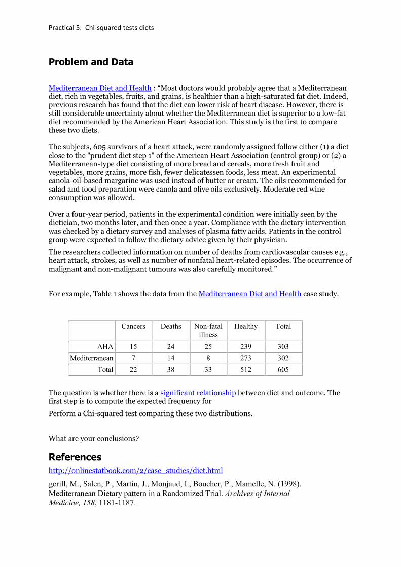
Mediterranean Diet and Health : “Most doctors would probably agree that a Mediterranean diet, rich in vegetables, fruits, and grains, is healthier than a high-saturated fat diet. Indeed, previous research has found that the diet can lower risk of heart disease. However, there is still considerable uncertainty about whether the Mediterranean diet is superior to a low-fat diet recommended by the American Heart Association. This study is the first to compare these two diets. The subjects, 605 survivors of a heart attack, were randomly assigned follow either (1) a diet close to the "prudent diet step 1" of the American Heart Association (control group) or (2) a Mediterranean-type diet consisting of more bread and cereals, more fresh fruit and vegetables, more grains, more fish, fewer delicatessen foods, less meat. An experimental canola-oil-based margarine was used instead of butter or cream. The oils recommended for salad and food preparation were canola and olive oils exclusively. Moderate red wine consumption was allowed. Over a four-year period, patients in the experimental condition were initially seen by the dietician, two months later, and then once a year. Compliance with the dietary intervention was checked by a dietary survey and analyses of plasma fatty acids. Patients in the control group were expected to follow the dietary advice given by their physician.
The researchers collected information on number of deaths from cardiovascular causes e.g., heart attack, strokes, as well as number of nonfatal heart-related episodes. The occurrence of malignant and non-malignant tumours was also carefully monitored.”
For example, Table 1 shows the data from the Mediterranean Diet and Health case study.
Cancers Deaths Non-fatal
illness
Healthy Total
AHA 15 24 25 239 303
Mediterranean 7 14 8 273 302
Total 22 38 33 512 605
The question is whether there is a significant relationship between diet and outcome. The first step is to compute the expected frequency for
Perform a Chi-squared test comparing these two distributions.
What are your conclusions?
References
http://onlinestatbook.com/2/case_studies/diet.html
De Longerill, M., Salen, P., Martin, J., Monjaud, I., Boucher, P., Mamelle, N. (1998).
Mediterranean Dietary pattern in a Randomized Trial. Archives of Internal
Medicine, 158, 1181-1187.

Practical 7: Kernel Regression Galton Family data
Practical 7: Kernel Regression Galton Family data
Exercise
1. Import the GaltonFamilies.csv data
2. Compute the midparent height
3. Compute a binary variable z = 1 if male height >= 70 inches
4. Fit a logistic regression to the binary variable z on midparent height
5. Get the summary and anova for the logistic regression. Interpret.
6. Plot the male data with its logistic regression regression line
7. Perform a kernel regression on these data for various bandwidths using a normal
kernel
8. Plot the male height vs midparent height and draw horizontal line at height of 70
inches, and vertical lines at the quartiles of midparent height.
9. Make a cross-tabulation of the male height cutting at 70 inches and at quartiles of
midparent heights
10. Compute probabilities that son’s height >= 70 inches from your cross tabulation
References
References The manual titled “An Introduction to R” located on the official R website at http://cran.r- project.org/doc/manuals/R-intro.pdf is the main reference used in the creation of this document. Other references, with hyperlinks, are documented in the relevant text passages.
Chambers, John M. (1977). Computational methods for data analysis. New York: Wiley. ISBN 0-471-02772-3.
Chambers, John M. (1983). Graphical methods for data analysis. Belmont, Calif: Wadsworth International Group. ISBN 0-534-98052-X.
Chambers, John M. (1984). Compstat lectures: lectures in computational statistics. Heidelberg: Physica. ISBN 3-7051-0006-8.
Becker, R.A.; Chambers, J.M. (1984). S: An Interactive Environment for Data Analysis and Graphics. Pacific Grove, CA, USA: Wadsworth & Brooks/Cole. ISBN 0-534-03313-X.
Becker, R.A.; Chambers, J.M. (1985). Extending the S System. Pacific Grove, CA, USA: Wadsworth & Brooks/Cole. ISBN 0-534-05016-6.
Becker, R.A.; Chambers, J.M.; Wilks, A.R. (1988). The New S Language: A Programming Environment for Data Analysis and Graphics. Pacific Grove, CA, USA: Wadsworth & Brooks/Cole. ISBN 0-534-09192-X.
Chambers, J.M.; Hastie, T.J. (1991). Statistical Models in S. Pacific Grove, CA, USA: Wadsworth & Brooks/Cole. p. 624. ISBN 0-412-05291-1.
Chambers, John M. (1998). Programming with data: a guide to the S language. Berlin: Springer. ISBN 0-387-98503-4.
Chambers, John M. (2008). Software for data analysis programming with R. Berlin: Springer. ISBN 0-387-75935-2.
Murrell, P. (2011). R graphics (2nd ed.). London, United Kingdom: Chapman & Hall.
R Development Core Team. (2015). R: A Language and Environment for Statistical Computing. Vienna, Austria: R Foundation for Statistical Computing. Retrieved from http://www.R-project.org
Tay, l., Parrigon S., Huang, Q., and James M. LeBreton2, J.M. (2016) Graphical Descriptives: A Way to Improve Data Transparency and Methodological Rigor in Psychology. Perspectives on Psychological Science 2016, Vol. 11(5) 692 –701, DOI: 10.1177/1745691616663875
Tufte, E. R. (1983/2000). The visual display of quantitative information. Cheshire, CT: Graphics Press.
Tufte, E. R. (1990). Envisioning information. Cheshire, CT: Graphics Press.
Tufte, E. R. (1997). Visual explanations. Cheshire, CT: Graphics Press.
Tufte, E. R. (2006). Beautiful evidence. Cheshire, CT: Graphics Press.
Wickham, H. (2010) A Layered Grammar of Graphics. Journal of Computational and Graphical Statistics, Volume 19, No 1, p 3-28, DOI: 10.1198/jcgs.2009.07098
Wickham, H. (2016) ggplot2: Elegant Graphics for Data Analysis (Use R!). Springer; 2nd ed.
Wilkinsin, L. (2005) The Grammar of Graphics (Statistics and Computing) Second Edition. Springer; 2nd ed.
References
Braun, W. J. and Murdoch, D. J. (2007) A First Course in Statistical Programming with R. CUP. Chambers (2010) - Software for Data Analysis: Programming with R, Springer. Crawley, M. (2007) The R Book. Wiley. Dalgaard, P. (2009) Introductory Statistics with R. Second Edition. Springer. Fox, J. (2002) A R and S-PLUS Companion to Applied Regression. Sage. Ligges, U. (2009) Programmieren mit R. Third edition. Springer. In German(!) Maindonald J. and Braun, W. J. (2003) Data Analysis and Graphics using R Second or third edition CUP. Rizzo, M. L. (2008) Statistical Computing with R. CRC/Chapman & Hall. Spector, P. (2008) Data Manipulation with R. Springer Venables, W.N. and Ripley, B.D. (2002) Modern Applied Statistics with S. Springer-Verlag. 4th edition. Wickham, H. (2014) Advanced R. Chapman and Hall.