data analysis from experimental measurements on a...

Master of Science Thesis KTH School of Industrial Engineering and Management

Energy Technology EGI_2017-0070-MSC EKV1196 Division of Heat & Power SE-100 44 STOCKHOLM

Data Analysis from Experimental Measurements on a Vertical Axis

Wind Turbine

Raphaël Coneau

Master of Science Thesis EGI_2017-0070-MSC EKV1196

Data Analysis from Experimental Measurements

on a Vertical Axis Wind Turbine

Raphaël Coneau

Approved

2017-08-15

Examiner

Miroslav Petrov - KTH/ITM/EGI

Supervisor

Miroslav Petrov Commissioner

Nenuphar Wind, France

Contact person

Denis Pitance

Abstract

This thesis presents the analysis of the data measured during the test campaign of a vertical axis wind turbine prototype developed by the company Nenuphar Wind in France. Three studies are presented: the study of the loads measured during the test campaign, the study of the vibrations, and the study of the stall conditions on the blades. Focus is put on the methodology of these analyses rather than on their detailed results.

The preliminary processing of data is presented in more details, in particular the determination of selection levels asserting the quality of the data, an analysis of the drift of the zero of the loads sensor and an analysis of the cross-talk effects on the same loads sensors. With reference to the experience gained on previous prototypes, the quality of the data acquired on this prototype was greatly improved, allowing the use of stricter selection levels and a better quality of the results. The drift of the zero of the strain gauges was identified to be caused by temperature effects and was corrected on most of the sensors, leading to a significant decrease of the uncertainty on the loads measurements. The analysis of the cross-talks led to the implementation of a new and more precise way of calculation of the uncertainty due to these effects.

Finally, the study of the dynamic stall on the blades of the new prototype developed by Nenuphar is described at the end of the report. The comparison with the previous prototype showed similar stall angular ranges, but less stalled rotations were observed on the new prototype than on the previous one.

-i-

Contents 1 Introduction .......................................................................................................................................................... 1

1.1 Background .................................................................................................................................................. 1

1.2 Presentation of the company .................................................................................................................... 3

1.2.1 Nenuphar-Wind ................................................................................................................................. 3

1.2.2 The prototypes ................................................................................................................................... 5

1.3 Methodology ................................................................................................................................................ 6

1.3.1 Objectives ............................................................................................................................................ 6

1.3.2 Methodology ....................................................................................................................................... 6

1.3.3 Scopes and limitations ....................................................................................................................... 6

2 TEST CAMPAIGN SUMMARY ..................................................................................................................... 8

2.1 Detailed presentation of the 1HS prototype .......................................................................................... 8

2.2 Test campaign summary .......................................................................................................................... 10

3 LOAD STUDY .................................................................................................................................................. 11

3.1 Presentation of the loads measurements ............................................................................................... 11

3.1.1 Strain gauges ..................................................................................................................................... 11

3.1.2 Zeroing of the strain gauges ........................................................................................................... 12

3.2 Preliminary work on the data .................................................................................................................. 13

3.2.1 Campaign validation ........................................................................................................................ 13

3.2.2 Selection levels .................................................................................................................................. 14

3.2.3 Zero drift ........................................................................................................................................... 16

3.2.4 Cross-talks ......................................................................................................................................... 27

3.3 Loads Results ............................................................................................................................................. 34

3.3.1 Presentation of the loads ................................................................................................................ 34

4 VIBRATION STUDY ...................................................................................................................................... 37

4.1 Presentation of the vibration measurements ........................................................................................ 37

4.2 Preliminary work on the data .................................................................................................................. 37

4.2.1 Operational modal analysis ............................................................................................................ 38

4.2.2 Verification of the possibly dangerous rotational speeds .......................................................... 38

4.3 Vibration results ........................................................................................................................................ 38

5 TUFT ANALYSIS: study of the dynamic stall ............................................................................................. 40

5.1 Dynamic stall ............................................................................................................................................. 40

5.2 Presentation of the tuft tests ................................................................................................................... 41

5.3 Results ......................................................................................................................................................... 44

5.3.1 Results on the 1HB prototype ....................................................................................................... 44

5.3.2 Comparison with the results on the 1HS prototype .................................................................. 50

-ii-

6 CONCLUSION ................................................................................................................................................. 53

References ..................................................................................................................................................................... 54

-iii-

SAMMANFATTNING

Detta examensarbete presenterar analysen av de mättningsvärden som uppnåddes under testkampanjen på en vertikalaxlad vindturbinprototyp utvecklad av företaget Nenuphar-Wind i Frankrike. Tre analyser har gjorts: först en studie av krafterna som mättes under testkampanjen, sedan en studie av vibrationerna och sist en undersökning av överstegringsgraden på bladen. Fokus ligger på metodiken för dessa analyser snarare än på deras detaljerade resultat.

Den preliminära bearbetningen som gjordes på testdata före dessa tre studier presenteras också härmed, i synnerhet bestämningen av urvalsnivåer som hävdar datakvaliteten, en analys av variationen av nollpunkten för töjningsgivare och en analys av krosstalkseffekterna på töjningsgivare. Tack vare erfarenheten av tidigare prototyper förbättrades kvaliteten på de data som erhållits på denna prototyp avsevärt, vilket möjliggör användningen av strängare urvalsnivåer och bättre resultatkvalitet. Variationen av nollpunkten för töjningsgivare identifierades för att orsakas av temperatureffekter och korrigeras på de flesta sensorerna, vilket leder till en signifikant minskning av osäkerheten vid lastmätningarna. Analysen av krosstalkseffekterna ledde till genomförandet av ett nytt och mer exakt sätt att beräkna osäkerheten.

Slutligen presenteras studien av den dynamiska stall på den nya prototypen som utvecklats av Nenuphar i slutet av denna rapport. Jämförelsen med den tidigare prototypen visade liknande stall-vinkelområde, men mindre stall-benägna rotationer observerades på den nya prototypen än på den föregående.

-iv-

List of Figures Figure 1: Estimated Renewable Energy Share of Global Electricity Production, end-2016 (REN21, 2017) 1 Figure 2: Wind Power Global Capacity and Annual Additions, 2006-2016 (REN21, 2017) ............................ 1 Figure 3: Wind Power Offshore Global Capacity, 2006-2016 (REN21, 2017) ................................................... 2 Figure 4: Evolution of the power coefficient with the tilt angle for vertical axis (VAWT) and horizontal axis (HAWT) wind turbines (NenupharWind, 2017) ...................................................................................................... 3 Figure 5: Pressure field for a single wind turbine (left) vs contra rotative wind turbines (right) (NenupharWind, 2017) ................................................................................................................................................. 4 Figure 6: Wake interaction with contra rotative design (NenupharWind, 2017) ................................................ 4 Figure 7: General description of the 1HS turbine .................................................................................................... 8 Figure 8: Test site configuration ................................................................................................................................. 8 Figure 9: Wheatstone bridge configuration ............................................................................................................. 11 Figure 10: Position of the strain gauges on the 1HS prototype ........................................................................... 12 Figure 11: Movements relative to the chord of the profiles ................................................................................. 12 Figure 12: False values on anemometers signals .................................................................................................... 14 Figure 13: Distribution of the bins for the different selection levels on the wind direction variation .......... 15 Figure 14: Loads statistics for the different selection levels ................................................................................. 15 Figure 15: SG_218Mx_raw and SG_318My_raw with night only condition, Uhub<5 m/s and RotSPd1<1rpm ............................................................................................................................................................ 17 Figure 16: SG_217My_raw with night only condition, Uhub<5 m/s and RotSPd1<1rpm ........................... 17 Figure 17: Variation of the air temperature measured at night, with no wind and at standstill ...................... 18 Figure 18: SG_218Mx_raw as a function of air temperature ............................................................................... 18 Figure 19: SG_218My_raw as a function of air temperature ............................................................................... 19 Figure 20: Effect of the daily temperature variation on SG_211My_raw .......................................................... 20 Figure 21: SG_318My_raw at standstill with (top) and without (bottom) night only condition ................... 21 Figure 22: Results of the linear regression on SG_118My_raw ........................................................................... 22 Figure 23:SG_217Mx_raw with (bottom) and without (top) zero drift correction .......................................... 23 Figure 24: SG_217Mx_raw with (bottom) and without (top) zero drift correction ......................................... 24 Figure 25: SG_218My with and without daily temperature variation correction .............................................. 25 Figure 26: Configuration for flap signal calibration. NB: the configuration for torsion signal calibration is very similar .................................................................................................................................................................... 28 Figure 27: Configuration for edge signal calibration ............................................................................................. 28 Figure 28: Representation of the loads statistics .................................................................................................... 34 Figure 29 : Example of the graphic of the 10 min statistic - standstill loads ..................................................... 35 Figure 30: Estimation of the loads using data fit ................................................................................................... 36 Figure 31: Position of the accelerometers on the 1HS prototype ....................................................................... 37 Figure 32: Example of the representation of the vibration statistics in operation ........................................... 39 Figure 33: Example of the representation of the vibration statistics at standstill ............................................. 39 Figure 34: Lift coefficient for static and dynamic stall .......................................................................................... 40 Figure 35: Angular ranges for static stall (left) and dynamic stall (right) ............................................................ 41 Figure 36: Tuft processing: Synchronization .......................................................................................................... 42 Figure 37: Tuft processing: cropping of the pictures ............................................................................................ 43 Figure 38: Tuft data acquisition ................................................................................................................................ 44 Figure 39: Stalled chord for one section (top) and for the whole blade (bottom) ............................................ 46 Figure 40: Stall and reattachment azimuthal positions for one section (top) and for the whole blade (bottom) ........................................................................................................................................................................................ 48 Figure 41: Stall detection on video ........................................................................................................................... 49 Figure 42: Stall positions as a function of the TSR ................................................................................................ 52

-v-

List of Tables Table 1: Azimuthal position relative to wind ............................................................................................................ 9 Table 2: Temperature corrections implemented on 1HS prototype ................................................................... 26 Table 3: Correction of the zero drift on the strain gauges .................................................................................... 27 Table 4: Comparison of the blade edge signal with and without cross-talk ...................................................... 30 Table 5: First estimation of the cross talk effects................................................................................................... 31 Table 6: Estimation of the transverse uncertainty ................................................................................................. 33 Table 7: Tuft tests on the 1HB prototype ............................................................................................................... 42 Table 8: Tuft processing: stall detection .................................................................................................................. 43 Table 9: Stall intervals for low, intermediate and high TSR ................................................................................. 49 Table 10: Stall and reattachment positions for 1HS and 1HB prototypes ......................................................... 51

-vi-

Abbreviations

DLC: Design Load Cases

FFT: Fast Fourier Transform

HAWT: Horizontal Axis Wind Turbine

IEPE: Integrated electronic piezoelectric

MLC: Measured Load Cases

MPPT: Maximum Power Point Tracking

OMA: Operational Modal Analysis

RPM: Rotation per minute

TSR: Tip Speed Ratio

Uhub: Wind speed at the hub height

VAWT: Vertical Axis Wind Turbine

-vii-

ACKNOWLEDGMENTS

First and foremost, I would like to thank my supervisor at Nenuphar-Wind Denis Pitance, as well as Pascal Beneditti. Their guidance and advices were a precious help all along this Master Thesis.

I would also like to thank the Test, Verification and Validation Team, and especially Joanna Kluczeswska-Bordier, for her supervision and her interest in my work.

I also want to thank the people working for Nenuphar-Wind in Aix-en-Provence for their warm welcome in their offices.

Finally, I would like to express my gratitude to my thesis supervisor at KTH Miroslav Petrov, thanks to whom this Master Thesis went off in the best conditions as possible.

-1-

1 INTRODUCTION

1.1 Background The share of renewable energies in the global energy production is rapidly increasing: an estimated capacity of 161 gigawatts (GW) was added to the global renewable energy capacity in 2016, which is the largest annual increase ever observed. (REN21, 2017) By the end of the year 2016, the estimated share of renewable sources in the global electricity production was estimated at 24.5%, hydropower representing the main part of it with 16.6% of the global electricity production. The second renewable electricity source is wind power, followed by bio-power and solar PV. The shares of these electricity sources are distributed as shown in Figure 1 below:

Figure 1: Estimated Renewable Energy Share of Global Electricity Production, end-2016 (REN21, 2017)

This rise can be explained by the decreasing price of the renewable energies which make them more and more competitive compared to fossil fuel generation and by the incentive policies introduced in the past years by the governments.

As shown before in Figure 1, wind power is the second largest renewable energy source after hydropower. By the end of 2016, the global wind power capacity was estimated at 487 GW. The evolution of the wind power global capacity over the past decade is presented in Figure 2 below:

Figure 2: Wind Power Global Capacity and Annual Additions, 2006-2016 (REN21, 2017)

Most of the wind power capacity comes from onshore wind power: offshore wind power accounted for less than 3% of the total wind capacity in 2016 with 14.4 GW installed, mostly in Europe. (REN21, 2017)

-2-

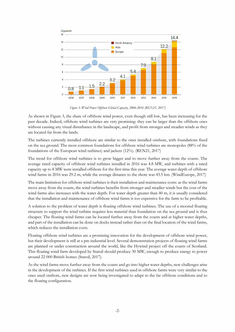
Figure 3: Wind Power Offshore Global Capacity, 2006-2016 (REN21, 2017)

As shown in Figure 3, the share of offshore wind power, even though still low, has been increasing for the past decade. Indeed, offshore wind turbines are very promising: they can be larger than the offshore ones without causing any visual disturbance in the landscape, and profit from stronger and steadier winds as they are located far from the lands.

The turbines currently installed offshore are similar to the ones installed onshore, with foundations fixed on the sea ground. The most common foundations for offshore wind turbines are monopoles (88% of the foundations of the European wind turbines) and jackets (12%). (REN21, 2017)

The trend for offshore wind turbines is to grow bigger and to move further away from the coasts. The average rated capacity of offshore wind turbines installed in 2016 was 4.8 MW, and turbines with a rated capacity up to 8 MW were installed offshore for the first time this year. The average water depth of offshore wind farms in 2016 was 29.2 m, while the average distance to the shore was 43.5 km. (WindEurope, 2017)

The main limitation for offshore wind turbines is their installation and maintenance costs: as the wind farms move away from the coasts, the wind turbines benefits from stronger and steadier winds but the cost of the wind farms also increases with the water depth. For water depth greater than 40 m, it is usually considered that the installation and maintenance of offshore wind farms is too expensive for the farm to be profitable.

A solution to the problem of water depth is floating offshore wind turbines. The use of a moored floating structure to support the wind turbine requires less material than foundation on the sea ground and is thus cheaper. The floating wind farms can be located further away from the coasts and at higher water depths, and part of the installation can be done on docks instead rather than on the final location of the wind farms, which reduces the installation costs.

Floating offshore wind turbines are a promising innovation for the development of offshore wind power, but their development is still at a pre-industrial level. Several demonstration projects of floating wind farms are planned or under construction around the world, like the Hywind project off the coasts of Scotland. This floating wind farm developed by Statoil should produce 30 MW, enough to produce energy to power around 22 000 British homes (Statoil, 2017).

As the wind farms move further away from the coasts and go into higher water depths, new challenges arise in the development of the turbines. If the first wind turbines used in offshore farms were very similar to the ones used onshore, new designs are now being investigated to adapt to the far offshore conditions and to the floating configuration.

-3-

1.2 Presentation of the company

1.2.1 Nenuphar-Wind

Nenuphar-Wind is a French company created in 2006 by Charles Smadja and Frédéric Silvert, whose aim is to develop and commercialize floating offshore vertical axis wind turbines. The company employs around 40 employees. Nenuphar-Wind was born in 2006 in Lille (France) where their first small-scale (35 kW) vertical axis wind turbine prototype was built. New offices opened later in Paris when the company started to work with Adwen (Areva), and in Aix-en-Provence (France) when a test site was opened in 2014 in Fos-sur-Mer, a close-by industrial harbor.

Nenuphar-Wind is developing a unique and innovative design for floating vertical axis wind turbines. Vertical axis wind turbines have not been widely used at an industrial scale, as horizontal axis wind turbines are considered to have better yields. They are mainly used onshore for small scale power generation, like residential applications in urban areas for instance. However, vertical axis wind turbines have some advantages over horizontal axis wind turbines, especially in the case of floating offshore wind turbines:

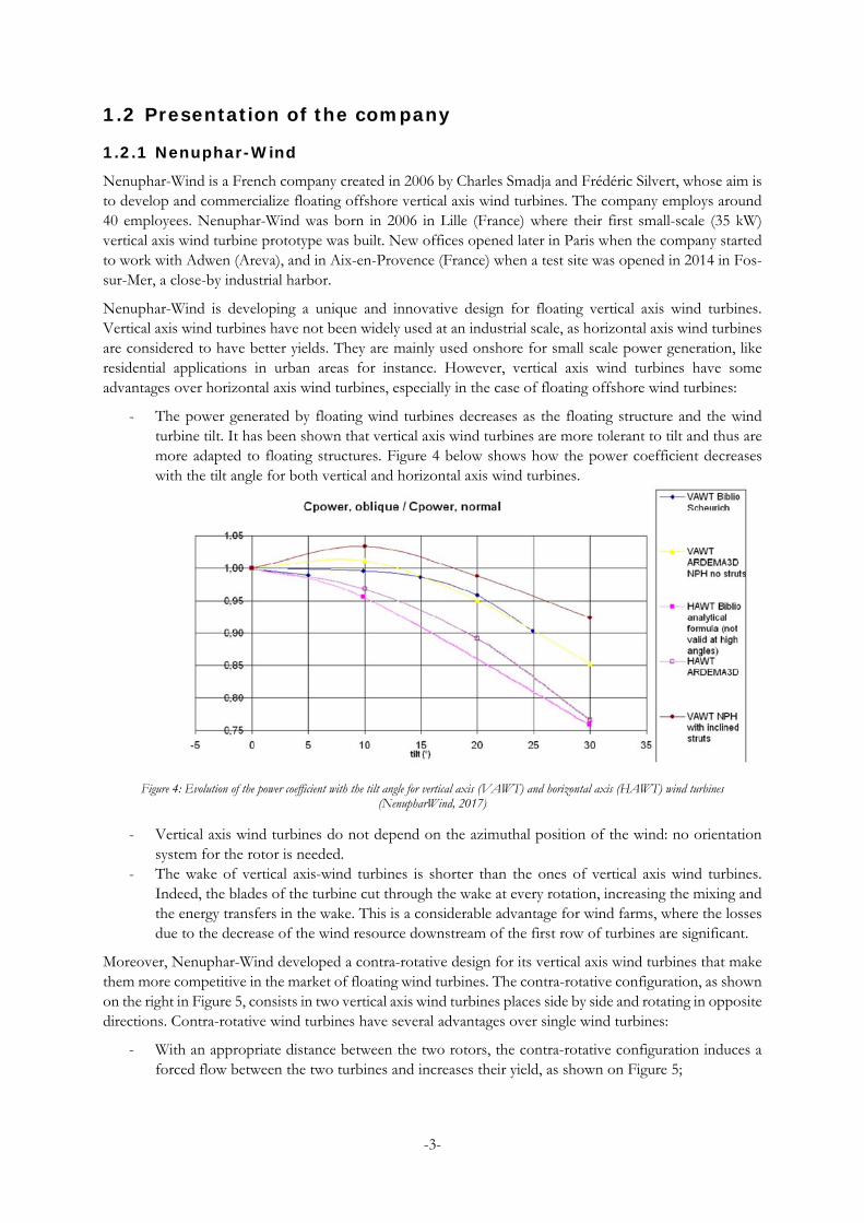
- The power generated by floating wind turbines decreases as the floating structure and the wind turbine tilt. It has been shown that vertical axis wind turbines are more tolerant to tilt and thus are more adapted to floating structures. Figure 4 below shows how the power coefficient decreases with the tilt angle for both vertical and horizontal axis wind turbines.

Figure 4: Evolution of the power coefficient with the tilt angle for vertical axis (VAWT) and horizontal axis (HAWT) wind turbines

(NenupharWind, 2017)

- Vertical axis wind turbines do not depend on the azimuthal position of the wind: no orientation system for the rotor is needed.

- The wake of vertical axis-wind turbines is shorter than the ones of vertical axis wind turbines. Indeed, the blades of the turbine cut through the wake at every rotation, increasing the mixing and the energy transfers in the wake. This is a considerable advantage for wind farms, where the losses due to the decrease of the wind resource downstream of the first row of turbines are significant.

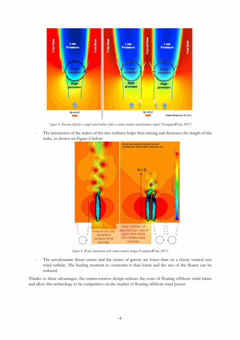
Moreover, Nenuphar-Wind developed a contra-rotative design for its vertical axis wind turbines that make them more competitive in the market of floating wind turbines. The contra-rotative configuration, as shown on the right in Figure 5, consists in two vertical axis wind turbines places side by side and rotating in opposite directions. Contra-rotative wind turbines have several advantages over single wind turbines:

- With an appropriate distance between the two rotors, the contra-rotative configuration induces a forced flow between the two turbines and increases their yield, as shown on Figure 5;

-4-

Figure 5: Pressure field for a single wind turbine (left) vs contra rotative wind turbines (right) (NenupharWind, 2017)

- The interaction of the wakes of the two turbines helps their mixing and decreases the length of the wake, as shown on Figure 6 below:

Figure 6: Wake interaction with contra rotative design (NenupharWind, 2017)

- The aerodynamic thrust center and the center of gravity are lower than on a classic vertical axis wind turbine. The heeling moment to overcome is thus lower and the size of the floater can be reduced.

Thanks to these advantages, the contra-rotative design reduces the costs of floating offshore wind farms and allow this technology to be competitive on the market of floating offshore wind power.

-5-

1.2.2 The prototypes

In parallel to the design of its wind turbines, Nenuphar-Wind is developing an aero-elastic code called PHARWEN, in cooperation with Adwen (Siemens Gamesa). Indeed, the codes used for classical wind turbines are not adapted to the simulation of the wind flow around vertical axis wind turbines: the wake is disturbed by the passing of the blades, and the angle of attacks constantly changes during a rotation, creating dynamic stall conditions that need to be precisely evaluated and simulated. In order to validate this code, Nenuphar-Wind has been operating several prototypes on the test site of Fos-sur-Mer.

The data acquired during the test campaigns of these prototypes are compared to the results of the code in the validation process, but they also give precious information to the design teams who can then adapt the design of the turbine to reduce the loads or increase the aerodynamic performances. The operation of a prototype is also a good way to gain experience for the development of future products and their commercialization.

Three different prototypes have been installed on the test site of Fos-sur-Mer, following the evolution of the design of the Nenuphar-Wind turbine:

The 1H prototype had three twisted blades and was supposed to be the first stage of a four stages helicoidal wind turbine. However, this design was abandoned as the twisted blades were costly to manufacture and induced high torsion loads in the struts. The 1H prototype was operating between May 2014 and June 2015

The 1HS prototype is the same as the 1H prototype but with straight blades that are lighter and easier to manufacture. The production cost of this turbine is lower than the one of the 1H, and so the cost of the energy produced is reduced. The 1HS prototype has been operating between July 2015 and October 2016.

The 1HB prototype has two straight blades equipped with a pitch angle control system which allows a control of the angle between the blade and the wind direction. It can easily be put in feathered mode, and the control of the pitch angle improves its aerodynamic performances. The 1HB prototype started its operation in January 2017 and was still in operation in July 2017.

In addition to these prototypes, Nenuphar-Wind is also working with universities, among which the Ecole Centrale de Nantes (France), TU Delft (Netherlands), VUB (Brussel) and Politecnico di Milano (Italy), to carry out wind tunnel tests in order to validate the contra-rotative designs and the control laws that cannot be validated with the current prototypes.

-6-

1.3 Methodology

1.3.1 Objectives

The work for this master thesis was carried out amongst the Test, Verification and Validation (TVV) team, managed by Joanna Kluczeswska-Bordier. The main supervisor for this thesis was Denis Pitance, working together with Pascal Beneditti, who are the members of the TVV team working on the site of Aix-en-Provence. The mission of the TVV team is to plan and carry out the tests needed for the validation of the PHARWEN code and of the design of the turbine. This includes both the tests on the prototypes and the wind tunnel tests.

In order to study the prototype installed on the test site of Fos-sur-Mer, strain and vibration sensors have been installed all over the structure of the turbine. Data are constantly acquired at a frequency of 50Hz, and transferred every day on the servers of Aix-en-Provence. A meteorological mast has also been installed close to the wind turbine to acquire meteorological data such as the wind speed, wind direction and air temperature

It is necessary to summarize the observations and analysis made during the test campaigns to gain experience from the prototypes and to communicate the results to the teams that will use the data for the code validation or for the improvement of the future turbines design in an efficient way. It was the objective of this master thesis to analyze the data acquired during the test campaign of the 1HS prototype, which ended in October 2016.

1.3.2 Methodology

The methodology on this master thesis was mainly guided by the company’s requirements. The analysis of the 1HS campaign was done in three steps, resulting in the writing of three internal documents, following the data analysis process already defined by the company:

- The first step of this work was the writing of a summary of the 1HS test campaign. The purpose of this document is to list the different major events that occurred on site during the prototype lifetime and to give an overview of the wind turbine operation and resulting test data available, stating issues and particular events that could have affected data quality and that should be taken into account when analyzing measurement data. It is a valuable source of information for people who wish to have a better understanding of the data acquired over the test campaign. The information presented in this document is summarized in chapter 2

- The second step of this work was the analysis of the loads measured during the 1HS test campaign. This analysis was presented in a load report whose objective is to present the results of the loads measurement as well as the methods of data selection and data cleaning and their influence on the results. The analysis of the loads and the preliminary work conducted before this analysis represent the main part of this master thesis. This analysis will be presented in chapter 3.

- The third step of this work was the analysis of the vibrations measured during the 1HS campaign. The work on the vibration analysis was mainly a summary of the measurements carried out during the campaign, and will only be presented briefly in this report. This analysis will be presented in chapter 4.

- Finally, an additional study of the dynamic stall effect on the blades was carried out on the 1HB prototype. The objective of this study was to compare the stall conditions on the 1HS and the 1HB prototype, following the methodology of a study that was already performed on the 1HS prototype in 2016. This work will be presented in chapter 5.

1.3.3 Scopes and limitations

The results of the different studies in this document were presented with an estimation of their uncertainties. The calculation of these uncertainties was done internally in the company prior to the start of this thesis,

-7-

and will not be explained in detail here. Some modifications and corrections concerning the computation of the uncertainties linked to the transvers effects on the load sensors were done during this master thesis. They will be presented in part 3.2.4 of this document.

The two main studies carried out during this master thesis were about loads and vibrations on the 1HS prototype. No results concerning the power production of the prototype will be given in this document, as they are part of another study internal to the company.

Finally, the reader should be aware that this report only gives selected information and data as the detailed results of the studies carried out during this master thesis should respect industrial confidentiality. No information regarding the wind turbine performances or its availability will be presented here, and only selected data will be presented for the measurements results. However, these selected data should be enough for the reader to understand the full results and trends observed during the test campaign of the 1HS prototype. The choice was made to focus this report on the analyses that could be presented in the most complete way, without any alteration or concealing of the data. This is why some studies carried out during this master thesis are only mentioned in this report with no detailed explanations of the work done or the results obtained, in order to avoid presenting incomplete results.

Some figures in this report are still presented without any axis information; they are only a way to show an observed trend or a choice of representation and not a support for a scientific analysis.

-8-

2 TEST CAMPAIGN SUMMARY

2.1 Detailed presentation of the 1HS prototype Before presenting the study of the 1HS prototype, it is necessary to give the reader a more detailed overview of the 1HS turbine. This section presents the main characteristics of the 1HS prototype and its instrumentation.

2.1.1.1 Geometry of the turbine

Figure 7 below show the main elements of the 1HS prototype:

Figure 7: General description of the 1HS turbine

The test site is located in South-Eastern France, in an industrial harbour located around 7 km west of the city of Fos-sur-Mer. The closest obstacles are buildings, wind turbines and coal piles stored nearby. A Met mast is installed at a distance of 5.4D of the turbine. Picture of the test site and information on the main wind directions can be found in Figure 8 below:

Figure 8: Test site configuration

2.1.1.2 Presentation of the measurements

The angular position RotPos of the turbine is measured in degrees. It is defined as the angle between the strut 102 and the north geographical direction (counter clockwise) (see Table 1).

Strut

Blades

Hub

Pylon containing: - Bearings - Generator - Braking system

Bracings

-9-

Rotor speed (RotSpd) and rotor acceleration (RotAcc) are calculated from the derivation of the encoder signals.

In order to study the variation of the loads over a rotation, the azimuthal position of the rotor relative to the wind has to be computed. The data used to compute the azimuthal position of the rotor are:

- the rotor azimuth sensor– angle between the strut 101 and the north direction (counter clockwise); - the wind direction measured on the met mast – angle between the north and the wind direction

(clockwise).

Table 1 below shows the calculation of the azimuthal position:

Table 1: Azimuthal position relative to wind

On site configuration Convention of the model

The Meteorological mast is a lattice guy-wired construction. Anemometers, wind vanes and temperature sensors are installed on this mast to measure the meteorological conditions.

The 1HS prototype is also instrumented with strain gauges to measure the loads on the structure and with accelerometers to measure the vibration levels. These measurements will be presented later in this document.

Instrumentation and measurements related to the control system and power measurements will not be presented in this document as they are not used in this study.

2.1.1.3 Recording of the data

All the data on the 1HS prototype are recorded at a frequency of 50Hz, excepted for the data from the Met mast that are recorded at a frequency of 1Hz. The data are recorded continuously every day, regardless if the turbine is in operation or not. Every 10 minutes starting from 00:00:00, the data are saved into csv files, creating what is called a bin. Every bin contains 10 minutes of data. At the end of every day, all the bins recorded during the day are sent to the servers in Aix-en-Provence for further analysis.

Strut101

Strut102 (instrumented)

Strut 103

Nor

Azimuthal position

relative to wind (+)

180°

Strut101

Strut102 (Instrumented)

Strut 103

Azimuthal position

relative to wind (+)

Wind

0°

90° 27

Azimuthal position relative to wind = RotPos3 + Wind Dir + 90 + 120 (deg)

-10-

2.2 Test campaign summary The test campaign summary was a document written for the company at the beginning of this thesis. Its purpose is to be a tool for someone wanting to use the data of the 1HS prototype to have a better understanding of what happened during this test campaign. Its main parts are:

- A presentation of the 1HS prototype and of the measurements similar to the one presented in the previous part;

- A presentation of the control strategy of the turbine. Several control strategy and adjustment were tested successively during the campaign: constant speed control / torque control / Maximum Power Point Tracking (MPPT).

- Statistics regarding the number of bins acquired and the different operational points studied during the campaign.

- A study of the different problems and limitations of the operating range that occurred over the campaign, explaining how these problems were solved and how they can impact the data.

-11-

3 LOAD STUDY The main goal of the loads measurement on the 1HS prototype is to be compared with the ones calculated by the code developed by Nenuphar. The loads measurements are also a way to monitor the structure of the prototype during the campaign.

3.1 Presentation of the loads measurements

3.1.1 Strain gauges

The loads on the 1HS prototype are measured using strain gauges. Strain gauges consist in small resistive elements oriented in a preferred direction and placed at the point where the load measurement is needed. When a load is applied at this point, the resistive element is deformed and its electrical resistance varies proportionally to the deformation. Using a proper calibration, the value of the deformation deduced from the resistance variation in the strain gauge can then be used to compute the value of the loads.

As the resistance variations measured by strain gauges are usually very low, the strain gauges are usually arranged in a Wheatstone bridge configuration, as shown in Figure 9 below:

Ri : variable resistor (strain gauges)

V: supply voltage

ΔEm: measured voltage

Figure 9: Wheatstone bridge configuration

In this configuration, the measured voltage can be expressed as: ∆ . , where δi

is the resistance variation in the strain gauge Ri. The opposite signs in this expression enable a correction of the parasitic effects such as temperature effects or deformations in a transverse direction.

The strain gauges have been placed on the structure in order to measure:

- The bending and torsion of the pylon (due to the aerodynamic thrust and the alternator torque); - The traction and compression in the bracings; - On the blades and on the strut: the flap bending, the edge bending and the torsion

The position of the different strain gauges on the 1HS prototype are shown on Figure 10 below:

-12-

Bending and torsion measurement (3 axis)

Flap bending measurement (1 axis)

Traction/compression measurements(1 axes)

Temperature measurement

Figure 10: Position of the strain gauges on the 1HS prototype

The chosen nomenclature for the loads measurements is the following:

The measured component refers to a referential where the x-axis follows the direction of the strut, the z-axis is vertical and the y-axis orthogonal to the x and z axis. The moments measured are called flap bending, edge bending and torsion. The flap bending moment is the moment related to the movements in a direction orthogonal to the chord of the profile, while the edge bending moment is the moment related to the movements in the direction of the chord, as shown on Figure 11 below. With these conventions, the edge bending moment on the blades will be the Mx moment, and the torsion moment will be the Mz moment. Similarly, the edge bending on the struts is the Mz moment and the torsion moment is the Mx moment. For both the blades and the struts, the flap bending moment is always the moment around the y axis.

Figure 11: Movements relative to the chord of the profiles

3.1.2 Zeroing of the strain gauges

For this campaign, the strategy for zeroing the strain gauge was to zero the gauges on the completely assembled prototype, at standstill and at “zero wind” conditions. Consequently, the gravitational loads (loads due to the own weight of the structure) are zeroed and are not present in the calibrated load.

It should be noted that the gravity loads are constant and do not depend on the rotor azimuth (contrary to a HAWT).

SG 118

SG 117

SG 317

SG 318

SG 217

SG 218 T 218 SG 211

SG 212

SG 3

SG 4

SG 5 SG 1

SG 2

SG_17MyR

Sensor Type

Position of the measurement Measured component

Redundant gauge (if applicable)

-13-

The strain gauges signals were zeroed at the beginning of the test campaign, at standstill condition, with very low wind speeds (< 3m/s at hub height; to avoid lift forces to be applied on blades and struts), during the night (to avoid temperature effect).

The gravitational loads of each strain gauge were evaluated theoretically from the beam model.

3.2 Preliminary work on the data Before analyzing the loads measurements acquired during the test campaign, it is necessary to make some pre-processing of the data, to avoid taking into account erroneous or non-representative data in the final study. This preliminary work is following the recommendations of the IEC specifications. (IEC TS 61400-13, 2001)

3.2.1 Campaign validation

Before studying the data acquired over the campaign, it must be checked to exclude erroneous recordings due to system acquisition failures or related to sensors defects for instance. The validation of the campaign was done by checking the statistics of the data on the different sensors to identify these erroneous values. An automatic pre-invalidation is done to help detect the data which do not meet predefined validity rules, but the final selection had to be done manually.

The main identified errors were the following:

- Problem in the acquisition: incorrect number of lines in the .csv files, recording of 2 bins in the same file…;

- Failure in the acquisition system: no data recorded for some time; - Offsets; - False signals due to sensor defects.

Some other issues were identified but not invalidated, like:

- The drift of the zero of the strain gauges. The zero of the strain gauges can vary over the year. This phenomenon is presented with more details in part 3.2.3.

- When the wind is too low, the wind vane and the anemometers can stay blocked, displaying false values. This is a normal effect, as long as it appears only at very low wind speeds and for short periods of time. Indeed, some amount of minimal wind speed is required to counter mechanical friction of the bearings of these instruments. In Figure 12 below, the anemometer A12NE records wind variations that A27SW and A12SW do not perceive:

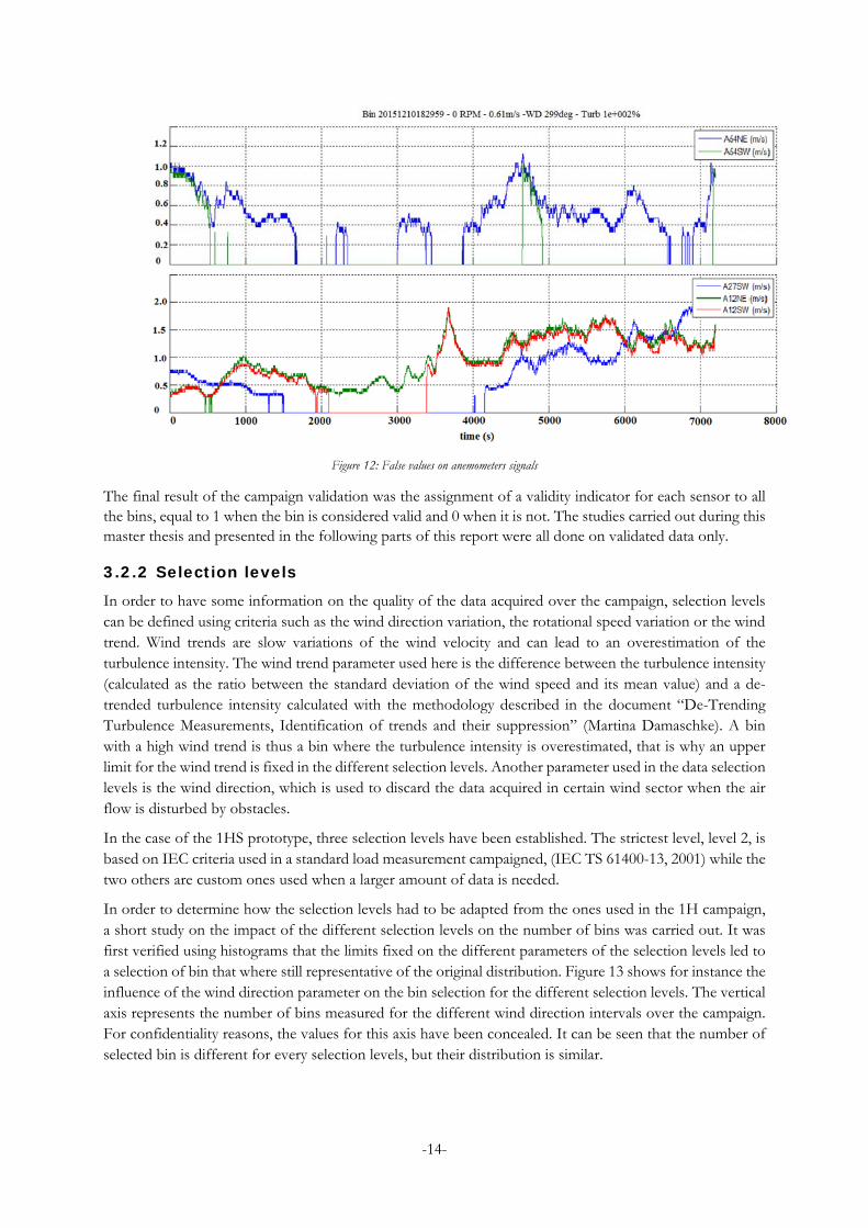
-14-

Figure 12: False values on anemometers signals

The final result of the campaign validation was the assignment of a validity indicator for each sensor to all the bins, equal to 1 when the bin is considered valid and 0 when it is not. The studies carried out during this master thesis and presented in the following parts of this report were all done on validated data only.

3.2.2 Selection levels

In order to have some information on the quality of the data acquired over the campaign, selection levels can be defined using criteria such as the wind direction variation, the rotational speed variation or the wind trend. Wind trends are slow variations of the wind velocity and can lead to an overestimation of the turbulence intensity. The wind trend parameter used here is the difference between the turbulence intensity (calculated as the ratio between the standard deviation of the wind speed and its mean value) and a de-trended turbulence intensity calculated with the methodology described in the document “De-Trending Turbulence Measurements, Identification of trends and their suppression” (Martina Damaschke). A bin with a high wind trend is thus a bin where the turbulence intensity is overestimated, that is why an upper limit for the wind trend is fixed in the different selection levels. Another parameter used in the data selection levels is the wind direction, which is used to discard the data acquired in certain wind sector when the air flow is disturbed by obstacles.

In the case of the 1HS prototype, three selection levels have been established. The strictest level, level 2, is based on IEC criteria used in a standard load measurement campaigned, (IEC TS 61400-13, 2001) while the two others are custom ones used when a larger amount of data is needed.

In order to determine how the selection levels had to be adapted from the ones used in the 1H campaign, a short study on the impact of the different selection levels on the number of bins was carried out. It was first verified using histograms that the limits fixed on the different parameters of the selection levels led to a selection of bin that where still representative of the original distribution. Figure 13 shows for instance the influence of the wind direction parameter on the bin selection for the different selection levels. The vertical axis represents the number of bins measured for the different wind direction intervals over the campaign. For confidentiality reasons, the values for this axis have been concealed. It can be seen that the number of selected bin is different for every selection levels, but their distribution is similar.

-15-

Figure 13: Distribution of the bins for the different selection levels on the wind direction variation

The impact of the selection levels on the data was then observed by plotting the loads statistic. In Figure 14 below, the loads statistics for one of the load sensors are shown for all three selection levels. For confidentiality reasons, the values of the loads as well as the values of the wind speed have been concealed. The black and red lines correspond to the average of all selected values for wind intervals of 1m/s. The red line is computed with the values of the level 0, the black line with crosses with the values of the level 1 and the black line with circles with the values of the level 2 . Every point represented on the graphs is a statistic computed for one 10-min bin: average value for the graph on the left, standard deviation for the graph in the middle and maximum/minimum relative to the average value for the graph on the right. The points with no filling are the points that are only selected by level 0, the points with a cross are the ones that are also selected with level 1 and the filled points are the ones that are also selected with level 2. More information on the choice of the loads statistics representation can be found in 3.3.1.

Figure 14: Loads statistics for the different selection levels

The average lines computed for the standard deviation as well as the maximum and minimum values are very close for the three selection levels. This means that the trend observed when selecting the data with selection levels 0, 1 or 2 should be very similar when performing the analysis of the loads for these statistic parameters. The difference observed between the three levels is more obvious in the case of the average values. The average lines observed for the selection levels 1 and 2 are still very similar, while the difference with the level 0 is greater. However, the trends observed are still close. This study shows that an analysis of

-16-

the results can be conducted with the different levels without a too significant difference in the results, even with the selection level 0.

This study also showed that the bins selected with the selection level 2 were in a sufficient number to be used in the study of the loads. The analysis presented in this document were all conducted using data with the selection level 2, unless specified otherwise.

In the end, the only criterion that was changed for the 1HS campaign was the wind direction criterion, with the addition of three new “forbidden” wind sectors where the wind turbine or the meteorological masts were in the wake of the surrounding buildings or of the close-by horizontal axis wind turbines.

3.2.3 Zero drift

3.2.3.1 Investigation on the zero drift during the 1HS campaign

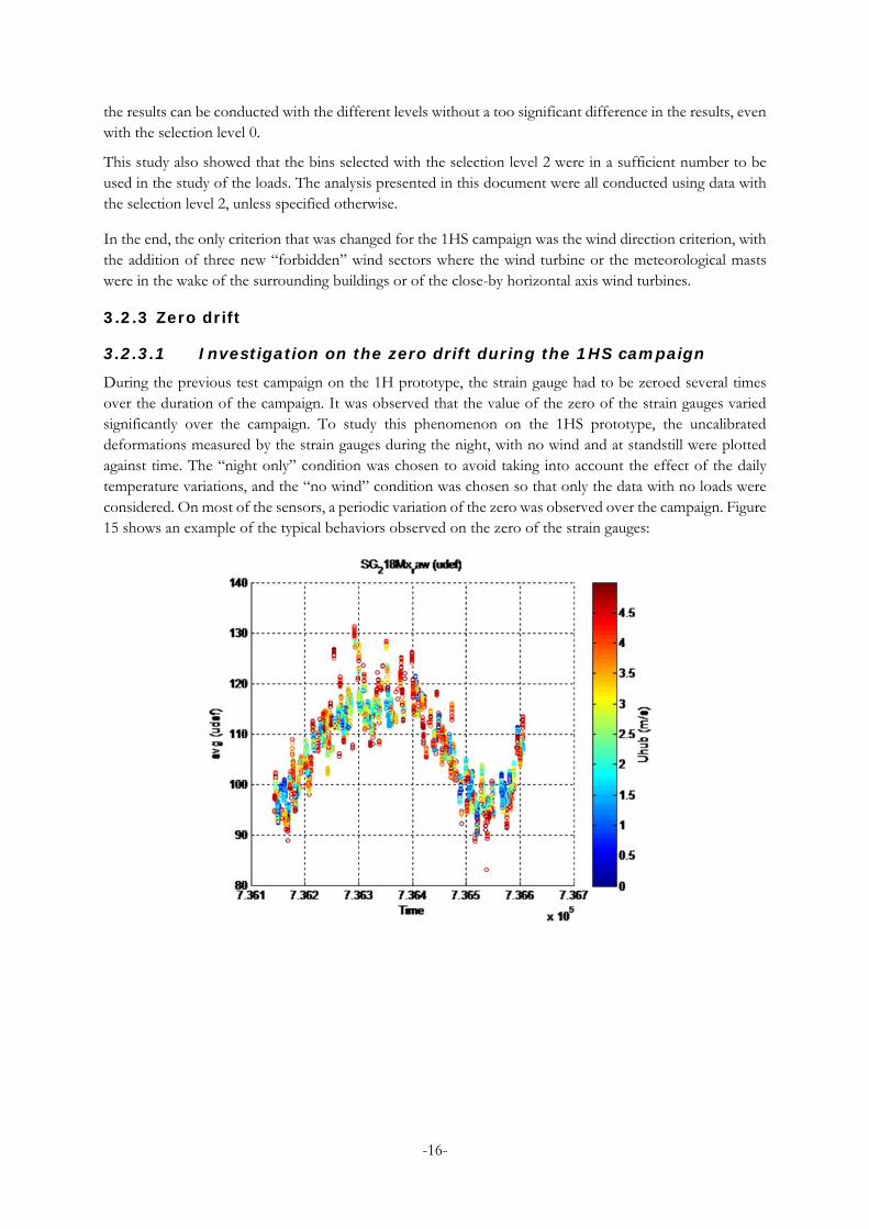
During the previous test campaign on the 1H prototype, the strain gauge had to be zeroed several times over the duration of the campaign. It was observed that the value of the zero of the strain gauges varied significantly over the campaign. To study this phenomenon on the 1HS prototype, the uncalibrated deformations measured by the strain gauges during the night, with no wind and at standstill were plotted against time. The “night only” condition was chosen to avoid taking into account the effect of the daily temperature variations, and the “no wind” condition was chosen so that only the data with no loads were considered. On most of the sensors, a periodic variation of the zero was observed over the campaign. Figure 15 shows an example of the typical behaviors observed on the zero of the strain gauges:

-17-

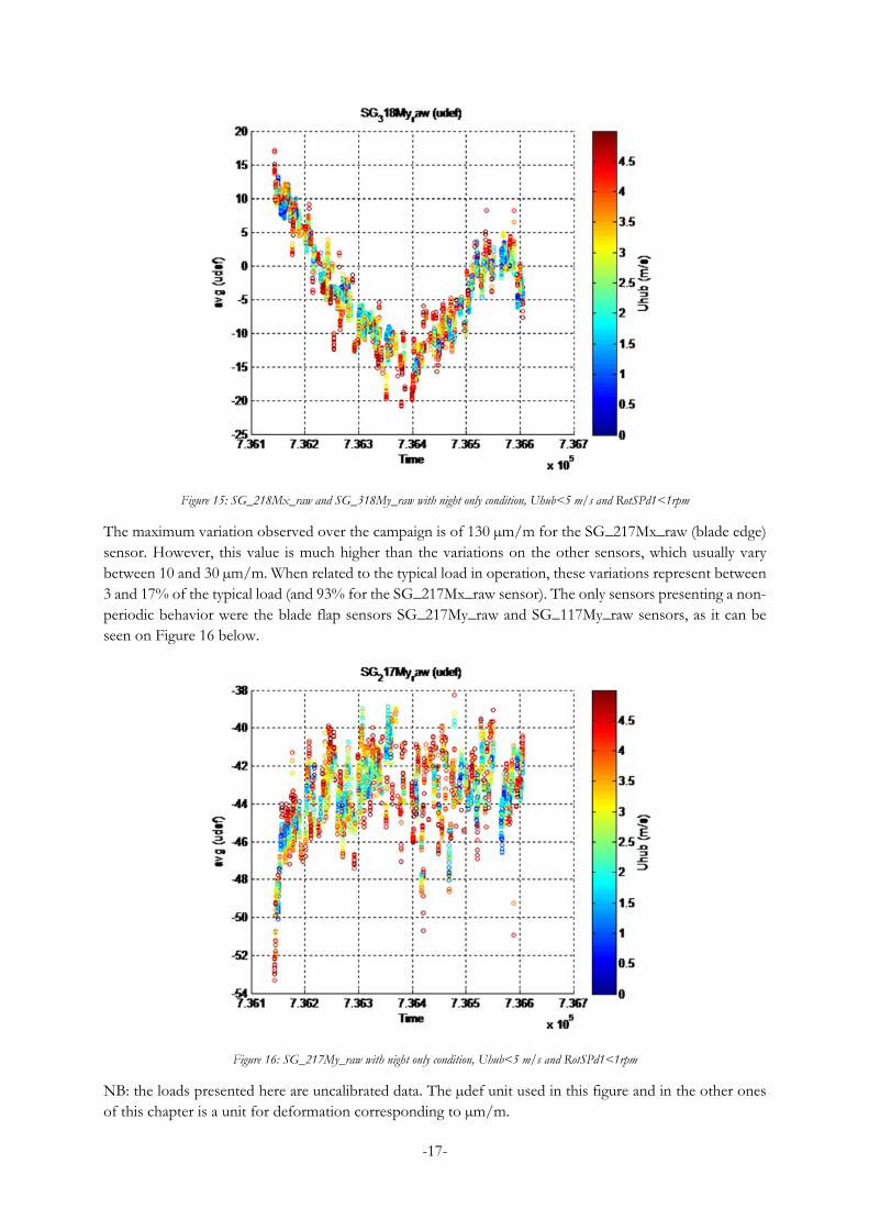
Figure 15: SG_218Mx_raw and SG_318My_raw with night only condition, Uhub<5 m/s and RotSPd1<1rpm

The maximum variation observed over the campaign is of 130 µm/m for the SG_217Mx_raw (blade edge) sensor. However, this value is much higher than the variations on the other sensors, which usually vary between 10 and 30 µm/m. When related to the typical load in operation, these variations represent between 3 and 17% of the typical load (and 93% for the SG_217Mx_raw sensor). The only sensors presenting a non-periodic behavior were the blade flap sensors SG_217My_raw and SG_117My_raw sensors, as it can be seen on Figure 16 below.

Figure 16: SG_217My_raw with night only condition, Uhub<5 m/s and RotSPd1<1rpm

NB: the loads presented here are uncalibrated data. The µdef unit used in this figure and in the other ones of this chapter is a unit for deformation corresponding to µm/m.

-18-

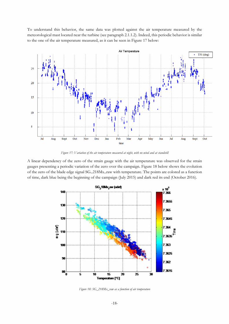
To understand this behavior, the same data was plotted against the air temperature measured by the meteorological mast located near the turbine (see paragraph 2.1.1.2). Indeed, this periodic behavior is similar to the one of the air temperature measured, as it can be seen in Figure 17 below:

Figure 17: Variation of the air temperature measured at night, with no wind and at standstill

A linear dependency of the zero of the strain gauge with the air temperature was observed for the strain gauges presenting a periodic variation of the zero over the campaign. Figure 18 below shows the evolution of the zero of the blade edge signal SG_218Mx_raw with temperature. The points are colored as a function of time, dark blue being the beginning of the campaign (July 2015) and dark red its end (October 2016).

Figure 18: SG_218Mx_raw as a function of air temperature

-19-

A hysteresis phenomenon was also observed on some of the sensors: when the temperature decreases and then increases again back to its original value, the sensors do not behave in the same way and two distinctive linear trends are observed. This can be observed for instance on the blade flap signal SG_217My_raw presented in Figure 19 below.

Figure 19: SG_218My_raw as a function of air temperature

The two sensors that did not show a periodic behavior over the campaign did not show a linear correlation with temperature either.

The conclusion of this first study on the drift of the zero of the strain gauges was that it is due to a temperature effect, and more specifically to the variation of the average air temperature over the year.

3.2.3.2 Temperature effects on strain gauges

The variations of temperature influence loads measurements by inducing thermal stresses in the material as the thermal expansion is different along the blades or the struts. This difference can be explained by an inhomogeneous temperature variation due to solar radiation, for instance when one side of the blade is exposed to the sun while the other side is in the shadow. (N.J.C.M Van Der Borg, 1998). The thermal stresses can also be explained by homogeneous temperature variation combined with different expansion coefficients of the material along the blade. The expansion or the contraction of the material with the temperature is usually corrected by the full bridge configuration of the strain gauge, as presented in 3.1.1. However, in the case of a composite material, the temperature expansion is not homogeneous in all directions. For composite materials, the temperature expansion can be almost null in the fiber direction, but significant perpendicularly to the fibers direction. The correction of the full bridge does not work as well then as in the case of a homogenous/isotropic material, like steel. (Rainer Klosse, 2006).

In the case of the 1HS prototype, the temperature influences the measurements in two ways: in a daily way when the solar radiation varies along the day, and in a seasonal way when the air temperature varies along the year.

The impact of the daily temperature variation was already studied during the 1H campaign. A clear correlation between the value of the loads at standstill and the hour of the day was observed, and is observed again on the 1HS prototype, as it can be seen for the strut flap signal SG_211My_raw in Figure 20 below:

-20-

Figure 20: Effect of the daily temperature variation on SG_211My_raw

The conclusion of this study was that it was not possible to correct the effect of this variation. But even if it leads to an important uncertainty value of the strain gauges, it does not affect the short term signal variation of the sensor. In other word, the average values of the loads measured during one rotation of the rotor are wrong, but the dynamic vibration amplitude and variations due to the aerodynamic loads stay correct. Moreover, a correction of this effect would require a knowledge of the temperature distribution on the whole blade and strut, and is thus impossible to put into practice with the current instrumentation on the 1HS prototype.

However, it is possible to correct the variations of the zero due to seasonal temperature variation as it depends mainly on the air temperature which is known. The correction of this temperature effect, i.e. of the drift of the zero investigated in the previous section, reduces the uncertainty on the average value of the strain gauges. Its implementation is presented in the following section.

Figure 21 below show the SG_318My_raw signal plotted over the campaign with and without the variations due to the daily temperature variations.

-21-

Figure 21: SG_318My_raw at standstill with (top) and without (bottom) night only condition

It has to be noted that the variations of the zero due to the seasonal temperature variations are of an order of magnitude 2 to 3 times lower than the ones due to daily temperature variations.

3.2.3.3 Temperature correction

To correct the drift of the zero due to the seasonal temperature variations, a linear regression was performed on the data to find an approximation of the signal of the form:

SG= intercept + slope1*Temperature + slope2*time,

-22-

The objective of the regression being to compute the coefficients intercept (constant coefficient), slope1 (regression coefficient for air temperature) and slope2 (regression coefficient for the time of the year) for each load sensor in order to correct their values.

The use of time in the regression enables to take into account the hysteresis phenomena, as it can be seen in Figure 22 below, where the black points are the ones estimated by the linear regression and the colored ones the measured data for the blade flap signal SG_118My_raw:

Figure 22: Results of the linear regression on SG_118My_raw

For the sensors on blade 2, the temperature used in the regression was the mean temperature of the blade (T_intrado + T_extrado)/2, while the air temperature is used for the sensors on blades 1 and 3. The blade temperature was indeed considered to be a more accurate parameter as it is the cause of the thermal expansion of the material, but could only be used on blade 2 since no temperature sensors were installed on blades 1 and 3.

The coefficients “intercept”, “slope1” and “slope2” were calculated using the Matlab software. The function “stepwisefit” was used to perform a linear regression on the load data using the air temperature and the time as input parameters. The SG value obtained was then subtracted to the original loads to correct the zero drift.

After correction, the dispersion is reduced and the point are more concentrated around constant levels for each rotational speed. This result is particularly visible on the sensor SG_217Mx_raw, which is the one with the highest temperature-induced zero drift. On Figure 23 below, the average loads measured in operation are presented with (right figure) and without (left figure) the zero drift correction:

-23-

Figure 23:SG_217Mx_raw with (bottom) and without (top) zero drift correction

The results of the correction can also be seen by plotting the average value of the loads against the rotational speed: the parabolic relation between the strain and the rotational speed (due to the centrifugal force) is more obvious after the correction, as it can be seen in Figure 24: SG_217Mx_raw with (bottom) and without (top) zero drift correction below:

Correction

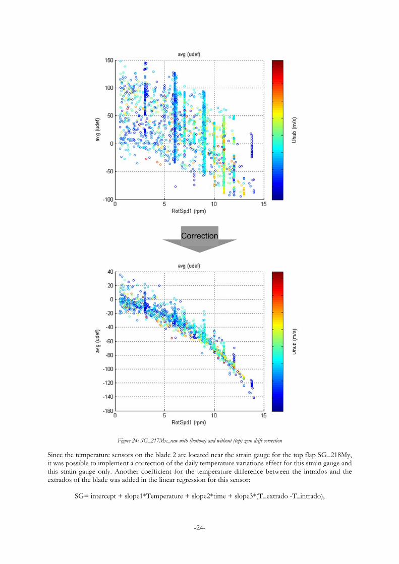
-24-

Figure 24: SG_217Mx_raw with (bottom) and without (top) zero drift correction

Since the temperature sensors on the blade 2 are located near the strain gauge for the top flap SG_218My, it was possible to implement a correction of the daily temperature variations effect for this strain gauge and this strain gauge only. Another coefficient for the temperature difference between the intrados and the extrados of the blade was added in the linear regression for this sensor:

SG= intercept + slope1*Temperature + slope2*time + slope3*(T_extrado -T_intrado),

Correction

-25-

Figure 25 below shows the effect of this correction on the zero of SG_218My: the figure on the left shows the uncorrected signal of the zero and the corrected signal without the daily correction, while the figure on the right shows the uncorrected signal and the corrected signal with the daily correction. It can be seen that the correction of the daily temperature variation effect reduces the variation of the signal around zero and thus reduces the uncertainty on the zero value.

Figure 25: SG_218My with and without daily temperature variation correction

However, the impact of the daily correction of the data in operation is quite low, as there is no significant improvement in the repartition of the data around constant rotational speed levels. This can be explained by the fact that the temperature on the surface on the blade is more homogeneous when the turbine is in rotation: the difference in temperature between the intrados and the extrados is usually below ±1°C while it can reach ±15°C at standstill.

-26-

Table 2 and Table 3below summarize the temperature corrections finally implemented on the strain sensors of the 1HS prototype:

Table 2: Temperature corrections implemented on 1HS prototype

Sensor name

Temperature correction

SG_117My SG_raw-zero (no temperature correction)

SG_118My SG_raw-( intercept + slope1*T51 +slope2*time)

SG_217Mx SG_raw-( intercept + slope1*T_mean +slope2*time)

SG_217My SG_raw-zero (no temperature correction)

SG_217Mz SG_raw-( intercept + slope1*T_mean +slope2*time)

SG_218Mx SG_raw-( intercept + slope1*T_mean +slope2*time)

SG_218My SG_raw-( intercept + slope1*T_mean +slope2*time

+ slope3*deltaT)

SG_318My SG_raw-( intercept + slope1*T51 +slope2*time)

With T_mean= (T_intrado+T_extrado)/2 and deltaT=T_intrado - T_extrado.

-27-

Table 3: Correction of the zero drift on the strain gauges

Zero interpolation

(determination of the correction law based on the interpolation of “night and low wind” measurement)

Variation of the zero of the strain gauge over the year:

Correlation with air

temperature

SGzero= intercept + slope1*Temperature + slope2*time (+ slope3*ΔT)

Zero correction

(application of the correction law to the loads in operation)

Uncorrected average loads

Corrected Loads =

Loads - SGzero

Corrected average loads

3.2.4 Cross-talks

When measuring a load in a specific direction, the strain gauge is measuring deformations in a specific direction. However, the load cell can also be sensitive to transverse deformations, and measure loads that are applied in a direction that is not the preferred one. This phenomenon is called a cross-talk, and is a source of error and uncertainty in the load measurements (N.J.C.M Van Der Borg, 1998). The cross-talk effects are usually quantified using the measurements carried out during the calibration process of the strain gauges.

3.2.4.1 Calibration of the strain gauges

In the case of the 1HS prototype, the calibration of the strain gauges on the blades was done in the following way:

- For the flap and edge signal calibration, a load was applied in the corresponding direction and a linear regression was then performed to link the response of the gauge to the applied load and obtain the calibration coefficients. The different configurations are presented in Figure 26 and Figure 27 below.

-28-

- As it was impossible to apply a pure torsion at the blade tips, the torsion signal calibration was done in the same configuration than the flap calibration but with the pulling out point out of the axis of the blade, as close as possible to the leading edge. As a result, the load applied is a combination of flap and torsion and is calibrated as such.

Figure 26: Configuration for flap signal calibration. NB: the configuration for torsion signal calibration is very similar

Figure 27: Configuration for edge signal calibration

The output of the calibration process are calibration matrices, which give the calibration coefficients to convert a load signal into a deformation signal. The non-diagonal components of these matrices represent the influence of the cross-talk effect.

During the calibration process, one cross-talk effect was clearly identified as the strain gauges installed for edge measurements responded to the loads in flap. This is due to the special bridge arrangement for the edge measurement. The cross-talks on the other strain gauges and other directions were considered to be zero, since the signals measured by the strain gauges other than the one being calibrated were low and below the accuracy of the calibration process.

A similar calibration process was carried out on the strain gauges of the strut. All the observed cross-talks were below 7% of the main signal and where thus neglected (ie not corrected) and taken into account as a source of uncertainty on the measurements which has to be evaluated.

3.2.4.2 First estimation of the impact of the cross-talks

The estimation of this uncertainty that was done so far was by fixing all cross-talk factors 7%, which is a maximum value chosen from the data of the calibration and found in the literature. This value was then propagated from the 50Hz data to the 10 min statistics in order to get one uncertainty value for every sensor and for every bin. However, the method of propagation led to an overestimation of the final uncertainty, with final uncertainties reaching values close or even higher than 100% for some sensors and some bins.

In order to determine if the uncertainty linked to the transverse effects, i.e. the non-inclusion of the cross-talks effects in the calibration, could be neglected, a first study was performed to see the influence of the cross-talks on the measurements.

The value of the signals calibrated with and without cross-talks were compared for 4 different bins and 4 different estimations of the cross-talks:

- Cross-talk 1: value measured during the calibration process (non-diagonal components of the calibration matrices);

- Cross-talk 2: same value than cross-talk 1 but with opposite signs;

-29-

- Cross-talk 3: twice as high as cross-talk 1; - Cross-talk 4: twice as low as cross-talk 1.

These values were chosen because the uncertainty on the value of the cross-talks measured during the calibration was high. This was a first way to have a quick estimation of how the cross-talk impacted the loads measurements.

Table 4 below shows the signals obtained for cross-talks 1 and 2 (in blue) compared to the one calibrated without cross-talks (in green) for one of the loads sensors.

-30-

Table 4: Comparison of the blade edge signal with and without cross-talk

X-talk 1

X-talk 2

These figures show that the different considered cross-talk all have an impact on the loads measurements. The next step of the analysis was to find a way to quantify this impact.

The estimation of the impact of the cross-talks should quantify how much the transverse effects influence the variations of the signal. A way to quantify the variation of a signal is to compute its standard deviation, which is defined as follow:

∑

-31-

Where avg is the average value of the N measurements Xi.

The standard deviation of the signal with the 4 different cross talks as well as the standard deviation of the signal without cross-talk were computed. These values show how much the signal vary during the chosen bin. In order to quantify how much these variations change when applying the different cross-talks, the standard deviation of the five computed standard deviations was calculated. Its value is an estimation of the standard uncertainty u on the standard deviation of the signal. The final uncertainty linked to this dispersion can be estimated by the expanded uncertainty U=k*u, where k is a coverage factor chosen as k=2. Table 5 below summarizes the process to calculate U.

Table 5: First estimation of the cross talk effects

No cross-talks

Standard deviation (variation of the signal)

u=Standard deviation (varitation of the variations of

the signals)

Expanded uncertainty U =2*u

Cross-talk 1


Cross-talk 2


Cross-talk 3


Cross-talk 4


-32-

This method was done for every load sensor, and the results obtained on the uncertainty were then compared to the ones already calculated by propagated cross-talk values of 7%.

This preliminary study confirmed that the impact of the transverse effect on the uncertainty was overestimated in its first estimation, and that is was not low enough to be neglected. Another method of uncertainty evaluation was thus needed in order to have a more realistic value of the uncertainty.

3.2.4.3 Estimation of the transverse uncertainty

The method used to evaluate the uncertainty linked to the transverse effects was the following:

For 8 bins, chosen for their variety in terms of conditions of operations, the uncertainty linked to the transverse effects was computed. This uncertainty was calculated in a similar way than in the previous part, but with a high number (N=104) of different cross talks values for every bin. These values where chosen in a random way in an interval between -7% and +7%.

For every sensor, the uncertainty evaluated in this study was of the same order of magnitude in the different bins. The final uncertainty value was chosen as the maximum value covering 75% of the 8 bins, in order to avoid an overestimation if one sensor had an anomalous behavior in one of the 8 bins. In this particular case, this means that the final uncertainty was the maximum one after rejecting the two highest values amongst the 8 values computed

Table 6 below summarizes the calculation process of the final estimation of the transverse uncertainty.

-33-

Table 6: Estimation of the transverse uncertainty

Bin n°1

Final uncertainty = maximum of the 8 bins without the 2 highest values

Cross-talk 1 (random between -7% and 7%)

Standard deviation (variation

of the signal)

u=Standard deviation (varitation of the variations of the signals)

Expanded uncertainty

U=2*u

.

.

.

Cross-talk N (random between -7% and 7%)


of the signal)

.

.

.

Bin n°8

Cross-talk 1 (random between -7% and 7%)


of the signal)

u=Standard deviation (varitation of the variations of the signals)

Expanded uncertainty

U=2*u

.

.

.

Cross-talk N (random between -7% and 7%)


of the signal)

NB: this study was only carried out on the sensors of blade n°2 only, which is the only one instrumented enough to evaluate the cross-talks. The uncertainties on the sensors on the blades n°1 and n°3 were deduced from the ones calculated on the blade n°2.

-34-

3.3 Loads Results

3.3.1 Presentation of the loads

The loads are studied for the operations at steady state, for transient events such as start-up and emergency stop, and at standstill. The focus of the study was made on the loads measured during steady state operation, as they will be the ones used for code validation. The study of the loads measured during transient events and at standstill is a way to have a better understanding of the prototype and its structure and to gain experience on the operation of vertical axis wind turbines.

3.3.1.1 Loads in operation

The loads on a vertical axis wind turbine are in general heavily related to the rotational speed because of the effects of the centrifugal forces. Moreover, the control mode of the 1HS prototype did not induce a direct relation between the wind speed and the rotational speed. Several controller setting were used in order to have a wide set of bins at different TSR, whatever the wind speed. As a result, the representation of the loads statistics chosen for this study is different from the one advised by the IEC (IEC TS 61400-13, 2001). Figure 28 below shows the chosen representation for the loads statistics: the loads are represented as a function of the wind velocity, colored with the rotational speed, and the average, standard deviation and extrema of the loads are presented on separated figures. For confidentiality reasons, all the axis data have been concealed in this figure. The purpose of this figure is to show the chosen representation of the loads and not to study these loads.

Every point on the figure below is a statistic value computed on one 10 minutes bin. The black curve corresponds to the average of all values for wind intervals of 1m/s. Representations of the uncertainties have also been added to the figures: the black arrow on the first plot represents the uncertainty on the value of the zero due to the seasonal and daily temperature variations, as explained in 3.2.3. The error bars on the average curve on the second plot correspond to the average of the uncertainty for wind intervals of 1m/s.

Figure 28: Representation of the loads statistics

The direct measurements of the loads (as opposed to the 10-minutes statistics presented above) were also studied for three selected bins. The loads for these bins were presented as time series, azimuthal representation and spectral representation.

3.3.1.2 Loads at standstill

The loads on the 1HS turbine were acquired all along the test campaign, whether the turbine was in operation or not. The data acquired at standstill are of little interest for the validation of the code. However, they can give information on the behavior of the structure at standstill and on the aerodynamic behavior of the blades.

The data used for the study of the loads at standstill was selected with the following rules:

- Wind data selection consistent to level 2

-35-

- Hour between 20:00 and 6:00: only the data recorded during the night is selected to reduce the temperature effect;

- Rotor Speed =0 RPM;

The same representation of the loads was used for the loads at standstill than for the loads in operation, with the only difference that the loads were colored as a function of the rotor azimuthal position rather than of the rotational speed.

Figure 29 : Example of the graphic of the 10 min statistic - standstill loads

3.3.1.3 Main observations on the loads study

The study of the loads is a way to study the performances of the wind turbine, to monitor the behaviour of its structure and to validate its design. Several analysis were made on the loads during this master thesis:

- A study of the loads statistics for every load sensors. - A comparison of the loads measured on the 1H and the 1HS prototypes. - A fit of the data using selected parameters. Only this last analysis will be presented here.

The fit of the data is a way to obtain an expression of the loads as a function of several chosen parameters such as the rotational speed, the wind speed, the turbulence intensity etc.:

∗ ∗ ∗ ⋯

This expression can be used to extrapolate the loads for given operational points, but also to see which parameters have more “weight” in the regression, i.e. the parameters that impact the loads the most.

The regression of the loads consist of a multilinear regression of a response variable Yn,1 (in this case, the loads) using a set predictor terms Xn,p defined by the user. The output is a set of parameters ap,1 such as Yn,1

= Xn,p* ap,1.

A first study on the choice of these parameters was carried out in the company before the beginning of this thesis, the main predictor terms being a set of constant, linear and quadratic terms formed with the rotational speed, the wind speed and the turbulence intensity. The final choice for the input parameters was adapted to take into account the first observations made on the loads. The air temperature was added in the input parameters to see the impact of the temperature on the sensors where it was not corrected (see 3.2.3.3). The standard deviation of the rotational speed was also added as an input parameter, while other parameters such as the shear coefficient were withdrawn from the parameter list as they did not seem to have a strong influence.

-36-

The data used for the regression was selected with the selection level 0 presented in 2.2. This level was chosen over a stricter one in order to keep as much information as possible on the influence of the chosen parameters, without strict constraints on these parameters.

The final parameters used for the different sensors were the following:

- Constant parameter; - Wind speed U; - Square of the rotational speed ω², to take into account the effects of the centrifugal forces; - ω*U and ω*U², to take into account the effects of the aerodynamic forces; - Turbulence intensity multiplied by wind velocity. This term was preferred over the turbulence

intensity alone to take into account the fact that the turbulence intensity tends to increase with the wind speed;

- The air temperature was also used as an input parameter for the sensors were the temperature correction presented in 3.2.3.3 was not implemented;

- Standard deviation of the rotational speed, to take into account the possible fluctuations of the rotational speed during the measurements.

Using the calculated coefficients, the value of the loads can be estimated for given values of the inputs. Figure 30 shows the result of the estimation of the loads using the regression parameters for three different rotational speeds for one of the load sensors. The values of the turbulence intensity, air density and air temperature were set as their average values over the test campaign. For confidentiality reasons, all the values from the axis have been concealed. The purpose of this figure is to show how the loads estimation from the data fit relates to the real loads rather than to study the loads themselves.

Figure 30: Estimation of the loads using data fit

For the sensor presented above, the fit of the data gives good results for the standard deviation and the maximum and minimum values: the loads estimated with the data fit manage to show the trend with the rotational speed that is observed. The fit of the data on the average values give constant load levels that are close to the average line already calculated.

-37-

4 VIBRATION STUDY The main goals of the study of the vibrations on the 1HS prototype are the surveillance of the dynamic behaviour of the structure and the verification of the modal parameters such as the vibration modes frequencies that were calculated with a finite elements code.

4.1 Presentation of the vibration measurements Only the rotor of the 1HS prototype has been instrumented with accelerometers as the pylon was considered to be rigid enough. The vibration measurements are made using Integrated Electronic Piezoelectric (IEPE) accelerometers. The piezoelectric effect is the ability for some materials to accumulate electric charge in response to mechanic stress. Piezoelectric accelerometers use this charge to measure vibrations. IEPE accelerometers are piezoelectric anemometers with a built-in amplifier. These accelerometers cannot measure the very low frequencies nor the constant accelerations; they can’t measure centrifugal acceleration and gravitational acceleration.

The position of the accelerometers on the 1HS prototype are presented on Figure 31 below:

1 accelerometer (1 axis)

2 accelerometers (2 axis)

Figure 31: Position of the accelerometers on the 1HS prototype

The chosen nomenclature for the loads measurements is the following:

The flap and edge vibrations refer to the same directions as the ones presented in the load study (see 3.1.1)

4.2 Preliminary work on the data No preliminary work on the vibration data was made during this master thesis. However, some studies on the dynamic behavior of the prototype were made in the company before the test campaign. They will be briefly presented here for a better understanding of the vibrations study.

A_S2_3B

A_S3_2M

A_S1_2M

A S2 1B

A_S2_2M

A_B2_4B

A_B2_5B A_B3_4B

A B1 5B

A_B3_5B

A_B3_4B

A_B1_5B1 Sensor Type

Position of the measurement BX : blade n° X SX : strut n° X

Measured component : B1 : blade flap\ strut edge B2 : blade edge\strut flap

Position of the measurement 1 : strut middle 2-3: strut tip 4 : blade bottom 5: blade tip

-38-

4.2.1 Operational modal analysis

The OMA (Operational Modal Analysis) consists in finding the structural modes parameters (frequencies, shapes, and damping factors) under the operational conditions, i.e. using the operational aerodynamic excitations in order to excite the structural modes. Contrary to an externally excited modal analysis (for instance, a hammer shock method), this method has the advantage of being able to identify the modal parameters of the particular structural modes that can be excited by the operational excitations (in terms of spatial shape, and time frequencies) with all the operational forces pre-stress effects (e.g. centrifugal stiffening). It has the drawback to give only normalized Frequency Response Functions (FRF) as the magnitude of the excitation is unknown.

The final result of the OMA is the list of the frequencies and corresponding damping factors for the edge, flap and torsion modes on the struts and the blades. The OMA also gives the shapes of these modes, i.e. the way the structure deforms when it is excited at the calculated frequencies.

4.2.2 Verification of the possibly dangerous rotational speeds

When the frequencies of the vibrations modes are known, it is good to verify that these frequencies are not reached during the operation of the turbine. Indeed, during the operation of the turbine, it is possible that the harmonics of the rotational speed (i.e. the multiples of the rotational speed) match the value of the frequencies of the vibrations modes. If this happen, the vibration modes can be excited and amplified, which can be a dangerous behavior for the structure of the turbine.

A test was performed to study these possibly dangerous operational points. The speed of rotation was slowly increased while monitoring the vibration levels. It was checked that no significant increase of the vibration levels was observed when the rotational speed or its harmonics reached the value of one of the frequencies of the vibration modes.

The result of this test was that no rotational speed was considered dangerous.

4.3 Vibration results The vibration results were presented in operation and at standstill. The presentation of the results is similar to the one of the loads. Vibration statistics are presented for the measurements both at standstill and in operation. In the case of the vibration measurements, vibration statistics are the 10-minute minimum, maximum and standard deviation values of the accelerometer signal: no statistic is computed for the average value as the average value of the vibrations should always be zero. The vibration statistics in operation are colored as a function of the rotational speed, while the statistics at standstill are colored as a function of the azimuthal position of the rotor. No uncertainty representation was added to the statistics representations. Figure 32 and Figure 33 below show an example the representations of the vibrations statistics in operation and at standstill. As for the loads study, the values on the axis have been concealed.

In the case of the vibration levels in operation, the power spectrum and time-series representation were also represented.

-39-

Figure 32: Example of the representation of the vibration statistics in operation

Figure 33: Example of the representation of the vibration statistics at standstill

The main study made on the vibration results was the analysis of the vibration levels as presented above. The vibration levels in operation showed how where the trends with the wind speed and the rotational speed, while the study of the measurements at standstill showed the impact of the rotor azimuthal position.

-40-

5 TUFT ANALYSIS: study of the dynamic stall

5.1 Dynamic stall Stall is a phenomenon that occurs on wing profiles at high incidence angles (usually from around 10° and higher) and is characterized by a brutal decrease of the lift and an increase of the drag. When the angle of incidence of the air flow on the profile is too high, a recirculation appears on the extrados of the profile. The boundary layer around the profile can then be divided into two separate parts, one where the flow is “attached” on the profile, and one where the flow is “detached”. The separation point xs moves along the chord c of the profile and gets closer to the leading edge as the angle of attack increases. When xs/c is lower than 75%, it is considered that the profile is stalled.

When the angle of attacks increases quickly before decreasing again, another stall phenomenon called dynamic stall, as opposed to static stall, can occur. Dynamic stall is also characterized by a decrease of the lift and an increase of the drag, but occurs for higher angles of incidence. The maximum reached by the lift is thus higher. When the angle of attack decreases again, the boundary layer reattaches for an angle of attack different than for the static case. Figure 34 below shows the evolution of the lift coefficient in the case of both static and dynamic stall:

Figure 34: Lift coefficient for static and dynamic stall

In the case of a vertical axis wind turbine with no pitch control, the conditions of apparition of dynamic stall are met as the angle of attack of the blades varies continuously during the rotation of the rotor. Stall occurs when the angle of attack of the relative wind W is high, where the relative wind velocity is the difference between the wind velocity and the velocity of the blade. This angle is high when the symmetry plane of the blade is perpendicular to the direction of the wind. This angular range is also the one where the wind is not a driving force on the blades. In the case of dynamic stall, the stall phenomenon is delayed and the angular ranges where it occurs are shifted. Figure 35 below shows the stall ranges for static and dynamic stall on a vertical axis wind turbine.

-41-

Figure 35: Angular ranges for static stall (left) and dynamic stall (right)

The angle of attack is not the only factor that has an impact on the stall. The Tip Speed Ratio (TSR), defined as the ratio between the velocity of the tip of the blades ωR and the wind velocity Uhub, also has a big influence on the angular ranges on which dynamic stall occurs. When the TSR is low, the wind velocity is high before the velocity at the tip of the blade, and the direction of the relative wind is close to the one of the incident wind. As a result, the angle of attack of the relative wind on the blade when the plane of symmetry of the blade is perpendicular to the wind is higher at low TSR than at high TSR: this is why the angular range where stall occurs is wider when the TSR is low. Moreover, when the TSR is high, i.e. when the rotational speed is high, stall does not occur necessarily at every rotation.

5.2 Presentation of the tuft tests A test campaign had already been carried out in 2016 to study the dynamic stall on the 1HS prototype through a video acquisition of tufts placed on one of the blades. A similar campaign was conducted on the 1HB prototype during this Master thesis in order to study the dynamic stall on the 1HB prototype and compare the results obtained for the two prototypes, that is to say to compare the results obtained when the number of blades is reduced from three to two for an otherwise similar configuration.

Tufts are little pieces of fabric usually fixed on a wing to detect stall. When the flow around the wing is undisturbed, the tufts are aligned with the direction of the flow, but when stall occurs, the flow around the wing becomes turbulent, and the movement of the tufts becomes erratic. It is a visual way to understand when and where the boundary layer around a wing or a profile becomes turbulent, which is often used on sailboats for instance. In the case of the 1HB turbine, tufts were placed regularly on five horizontal sections of one of the blades, each section containing five tufts. A camera facing the blade was placed on the strut.

Table 7 below shows the tufts on the blades as seen by the camera, a representation of the position of the camera and a close up on one of the tufts.

NB: only the upwind stall can be detected here, as the downwind stall occurs on the intrados of the blade (defined in this case as the side of the blade facing the outside of the turbine), while the video acquisition is only made on the extrados (defined as the side of the blade facing the pylon).

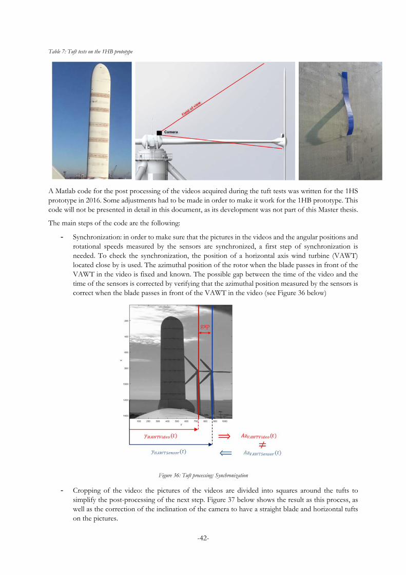
-42-

Table 7: Tuft tests on the 1HB prototype

A Matlab code for the post processing of the videos acquired during the tuft tests was written for the 1HS prototype in 2016. Some adjustments had to be made in order to make it work for the 1HB prototype. This code will not be presented in detail in this document, as its development was not part of this Master thesis.

The main steps of the code are the following:

- Synchronization: in order to make sure that the pictures in the videos and the angular positions and rotational speeds measured by the sensors are synchronized, a first step of synchronization is needed. To check the synchronization, the position of a horizontal axis wind turbine (VAWT) located close by is used. The azimuthal position of the rotor when the blade passes in front of the VAWT in the video is fixed and known. The possible gap between the time of the video and the time of the sensors is corrected by verifying that the azimuthal position measured by the sensors is correct when the blade passes in front of the VAWT in the video (see Figure 36 below)

Figure 36: Tuft processing: Synchronization

- Cropping of the video: the pictures of the videos are divided into squares around the tufts to simplify the post-processing of the next step. Figure 37 below shows the result as this process, as well as the correction of the inclination of the camera to have a straight blade and horizontal tufts on the pictures.

-43-

Figure 37: Tuft processing: cropping of the pictures

- Stall detection: the main part of the code is the stall detection. The pictures of the tufts are set in black and white and contrasted so that for each picture, the color difference between the tuft and the blade is maximal. This must be done for every picture independently as the lightning of the blade changes continuously during a rotation. The pictures are then converted into binary images where the tufts are set in white and the blade background in black (see Table 8 below). The condition for the tuft to be considered stalled is made on the value of the sum of the number of white pixels on every horizontal line of the picture: if this value is below a fixed limit, the tuft is not in a horizontal position anymore and is considered stalled. The results for each tuft and each picture of the videos are stored in binary vectors.

Table 8: Tuft processing: stall detection

Original tuft picture

Contrast adjustment

Final binary image

- Stall results: using these binary vectors, stall statistics can be computed. A chord line of tufts was considered stalled when 75% or more tufts on this line were stalled. The final results for the stall and reattachment azimuthal positions are presented in the form of pie charts (see 5.3 for some examples)

The tuft tests on the 1HB prototype were carried out on the 6th of June 2017. During the day, the rotational speed of the turbine was adapted as a function of the wind speed in order to record at least three bins of data at three chosen TSR. Figure 38 below shows the measurements of the wind speed, rotational speed and the corresponding TSR during these tuft test. It shows how the rotational speed was adapted to the

-44-

wind speed to get different values of TSR during the data acquisition. For confidentiality reasons, the values of the wind speed and of the TSR have been concealed.

Figure 38: Tuft data acquisition

The chosen TSR were the same as the ones used in the study made on the 1HS prototype. For confidentiality reasons, the value of the TSR will not be given here and will be referred to as “low”, “intermediate” and “high” TSR.

No pitch was applied on the blades of the 1HB prototype during the tests so that the configuration was as close as possible from the one of the 1HS. More tests with different pitch angles are planned in the future to see the impact of the pitch on the stall.

5.3 Results

5.3.1 Results on the 1HB prototype

The stall and reattachment azimuthal positions are calculated for every tuft section, before being averaged on the whole blade. The percentage of the chord that is stalled is computed for every rotation and is then

-45-

averaged to a final value (see

Figure 39 below).

-46-

Figure 39: Stalled chord for one section (top) and for the whole blade (bottom)

-47-

The results are then presented in the form of pie charts to get a visual representation of the stall and reattachment positions (see

Figure 40 below).

-48-

Figure 40: Stall and reattachment azimuthal positions for one section (top) and for the whole blade (bottom)

The validity of the results is checked by looking at the videos: for every TSR, a video is created showing the square areas around the tufts in green or red whether the tufts are stalled or not. Figure 41 below shows a picture of one of these videos where some tufts are detected as stalled while some are still attached. These videos are used to check if the tufts are stalled when they are calculated as such by the Matlab scripts.

Figure 41 below shows the apparition of stall on a rotation at low TSR. On the first picture on the left, all the tufts are horizontal: there is no stall. It can be noted that one of the squares is still in red, this is an error in the detection that is corrected later in the post processing by detecting the isolated stalled tufts. On the second picture, some of the tufts are stalled while others are still horizontal. In this case for instance, the tuft section at the top of the blade will be considered as stalled, while the one on the bottom will be

-49-

considered as still attached since less than 70% of its chord is stalled. The last picture on the right shows the fully stalled blade.

Figure 41: Stall detection on video

The average azimuthal ranges where stall is detected can then be compared for the different measured TSR. Table 9 below shows the comparison of the different TSR:

Table 9: Stall intervals for low, intermediate and high TSR

Low TSR

Intermediate TSR

-50-

High TSR

As expected, the azimuthal range where stall is observed gets narrower when the TSR increases. Another interesting observation is that when the TSR increases, dynamic stall does not occur on every rotation. For the low and intermediate TSR, dynamic stall occurs on every rotation, while it only occurs on 55% of the rotations for the high TSR.

5.3.2 Comparison with the results on the 1HS prototype

A similar test campaign had been conducted on the 1HS prototype for the same TSR in August 2015 and April 2016. The results on the 1HS campaign were also compared with numerical results obtained using the aerodynamic code Ardema, developed by Adwen in cooperation with Nenuphar Wind. These numerical results were computed with the 2D version of this code. They are compared here with the ones obtained on the 1HB prototype.

Table 10 below shows the stall and reattachment azimuthal positions for the different considered TSR for both 1HS and 1HB prototypes.

-51-

Table 10: Stall and reattachment positions for 1HS and 1HB prototypes

TSR 1HS 1HB

Low

Intermediate

High

NB: the reattachment position could not be calculated properly for the low TSR on the 1HS test because of shadow effects on the blades.

-52-

The azimuthal ranges for which stall is detected are very similar between the two prototypes. It seems that the air flow reattaches sooner on the 1HB prototype than on the 1HS, but the difference is too small for this conclusion to be certain.

Figure 42 below shows the stall and reattachment position as a function of the TSR for both the 1HS and 1HB prototypes, as well as the ones calculated by Ardema. In order to improve the comparison with the numerical results, the TSR measured on the two prototypes were corrected to take into account the shear effects on the wind, i.e. the fact that the wind velocity varies with the altitude. The wind velocity used in the calculation of these corrected TSR was calculated from the wind velocity measured at hub height using the following power law:

∗

Where α is a shear coefficient calculated from the values of the wind speeds measured over the day of the tuft test on the different anemometers of the meteorological mast, Uref is the wind velocity measured at the hub height zref and U is the wind speed at the height z of the middle tuft section.

Figure 42: Stall positions as a function of the TSR

This graph confirms the fact that the behavior of the air flow around the blades is very similar between the two prototypes: the difference between the results is of the order of magnitude of the dispersion of the points around the values estimated by the Ardema code.

-53-

6 CONCLUSION Over the course of this master thesis, a complete study of the test campaign on the 1HS vertical axis wind turbine prototype was carried out. The experience of the previous 1H prototype helped for a better execution of the test campaign, resulting in a much higher number of bins recorded. As a result, it was possible to apply stricter selection levels on the data recorded during the 1HS test campaign than during the 1H one. The data selected has a better quality, which is better for the code validation.

The study of the loads gave a better understanding of the behavior of the structure of the prototype in operation and at standstill. Improvements were made on the calculation of the transverse uncertainties caused by the cross-talk effects. The temperature influence on the strain gauges was also identified and corrected on most of the sensors. The observation of the loads was also a way to identify, analyze and gain experience for the next test campaigns.

The vibration study was a way to check the behavior of the structure of the turbine. Thanks to the high number of bins measured and of their better quality, the trend of the vibrations observed with the wind speed and with the rotational speed were much more obvious on the 1HS than on the 1H prototype.

Finally, the tuft tests and the analysis of their results were a way to have a better understanding of the phenomenon of the dynamic stall and of the air flow around the blades on both 1HS and 1HB prototypes. The same trends were observed for the two prototypes: a decrease of the angular range where stall appears when the TSR increases, as well as a decrease of the number of rotations where stall occurs. The stall and reattachment positions measured on both prototypes were also very similar for the same TSR.

The final outcome of this Thesis were three internal reports: the Test Campaign Summary of the 1HS test campaign, the Measured Loads report and the Measured Vibrations report, as well as a report on the tuft and dynamic stall analysis. These documents will be used by the code validation team as well as by the people who will need to refer to the events and measurements that occurred during the test campaign of the 1HS prototype. Another report on the power performances of the 1HS prototype should be written soon to complete the analysis of the test campaign.

The studies and information gathered over the analysis of the 1HS test campaign will also be a precious experience for the test campaign of the 1HB prototype, which started in January 2017. The main differences between the 1HS and the 1HB prototypes are the number of blades which decreased from three to two and the dynamic pitch system whose aim is to keep an optimized angle of attack on the blades and avoid dynamic stall. The 1HB prototype should be the last onshore prototype of Nenuphar-Wind before the installation of its first offshore turbines.

-54-

REFERENCES Most of the documents used during this Master Thesis were internal documents from Nenuphar-Wind. Only the external sources are referred to here.

IEC TS 61400-13. 2001. Technical Specification - Wind turbine generator systems - Part 13: Measurement of mechanical loads. 2001.

Martina Damaschke, Kai Mönnich, Holger Söker. De-Trending Turbulence Measurements, Identification of trends and their suppression. s.l. : Deutsches Windenergie Institut. 33546_DEWI.

N.J.C.M Van Der Borg, J.J.D Van Dam. 1998. The experimental quantification of specific uncertainty sources in wind turbine blade load measurements. 1998. ECN-C-97-105.

NenupharWind. 2017. La Twinfloat. www.nenuphar-wind.com. [Online] 2017. www.nenuphar-wind.com/fr/22-la-twinfloat.html.

Rainer Klosse, Holger Söker, Theo Kramkowski. 2006. Temperature Induced Drift in Mechanical Load Measurements on Wind Turbines. Wilhelmshaven : Deutsches Windenergie Institut, 2006.

REN21. 2017. Renewable 2017 Global Status report. 2017. ISBN 978-3-9818107-6-9.

Statoil. 2017. New energy solutions. statoil.com. [Online] 2017. www.statoil.com/en/what-we-do/new-energy-solutions.html.

WindEurope. 2017. The European Offshore Wind Industry - key trends and statistics 2016. 2017.

data analysis from experimental measurements on a...

Documents