darcytools v2.1 user guide
TRANSCRIPT

R-04-20
Svensk Kärnbränslehantering ABSwedish Nuclear Fueland Waste Management CoBox 5864SE-102 40 Stockholm SwedenTel 08-459 84 00
+46 8 459 84 00Fax 08-661 57 19
+46 8 661 57 19
DarcyTools, Version 2.1User´s guide
Urban Svensson,
Computer-aided Fluid Engineering AB, Sweden
Michel Ferry, MFRDC, France
March 2004

DarcyTools, Version 2.1User´s guide
Urban Svensson,
Computer-aided Fluid Engineering AB, Sweden
Michel Ferry, MFRDC, France
March 2004
ISSN 1402-3091
SKB Rapport R-04-20
This report concerns a study which was conducted in part for SKB. Theconclusions and viewpoints presented in the report are those of the author(s)and do not necessarily coincide with those of the client.
A pdf version of this document can be downloaded from www.skb.se

_____________________________________________________________________________________________ DarcyTools 2.1
Preface
The User’s Guide for DarcyTools V2.1 is intended to assist new users of DarcyTools. The Guide is far from complete and it has not been the ambition to write a manual that answers all questions a user may have.
The objectives of the Guide can be stated as follows:
- Give an overview of the code structure and how DarcyTools is used.
- Get familiar with the “Compact Input File”, which is the main way to specify input data.
- Get familiar with the “Fortran Input File”, which is the more advanced way to specify input data.

_____________________________________________________________________________________________ DarcyTools 2.1
Table of content Page
1 Introduction 1 1.1 Background 1 1.2 Objective 1 1.3 Intended use and user 1 1.4 Outline 2
2 What DarcyTools does 3 2.1 Situation in mind 3 2.2 Key features 5 2.3 Limitations 5
3 How DarcyTools operates 6 3.1 Introduction 6 3.2 General structure 6 3.3 Mathematical model 8 3.4 Finite volume equations and solver 10 3.5 Grid arrangements 10 3.6 Hardware, OS, etc 13 3.7 Directories, files and scripts 13
4 Compact Input File (CIF) 15 4.1 Introduction 15 4.2 Commands 19
5 Property Generation (prpgen.f ) 77
6 Fortran Input File (fif.f ) 80 6.1 Why needed? 80 6.2 How to use 80 6.3 Examples of use 89
7 A SITE LABORATORY-EXPERIMENTAL SCALE DEMO 95 7.1 Introduction 95 7.2 The situation studied 95 7.3 The set-up 98
8 References 115
9 Notation 116
Appendix A User Subroutines
Appendix B Structure of Solve
Appendix C Four CIF-examples

_____________________________________________________________________________________________ DarcyTools 2.1 1
1 Introduction 1.1 Background DarcyTools is a computer code for simulation of flow and transport in porous and/or fractured media. The fractured media in mind is a fractured rock and the porous media the soil cover on the top of the rock; it is hence groundwater flows, which is the class of flows in mind. DarcyTools is developed by a collaborative effort by SKB AB (The Swedish Nuclear Waste Management Company AB ) and CFE AB (Computer-aided Fluid Engineering AB). It builds upon earlier development of groundwater models, carried out by CFE AB during the last ten years. In this earlier work the CFD code PHOENICS (Spalding, 1981) was used as an equation solver. DarcyTools is based on a solver called MIGAL (Ferry, 2002). It has however been carefully evaluated that the two solvers produce very similar solutions and the earlier work is thus still valid as a background for DarcyTools.
The present report will focus on the software that constitutes DarcyTools. Two accompanying reports cover other aspects:
- Concepts, Methods, Equations and Demo Simulations (Svensson et al. 2004) (Hereafter Report 1).
- Verification and Validation (Svensson, 2004) (Hereafter Report 2).
Two basic approaches in groundwater modelling can be identified; in one we define grid cell conductivities (sometimes called the continuum porous-medium (CPM) approach, Jackson et al., 2000), in the other we calculate the flow through the fracture network directly (DFN approach). Both approaches have their merits and drawbacks, which however will not be discussed here (for a discussion, see Sahimi, 1995). In DarcyTools the two approaches are combined, meaning that we first generate a fracture network and then represent the network as grid cell properties. Further background information is given in the two reports mentioned.
1.2 Objective The main objective of this User’s Guide is to introduce and explain all parts of DarcyTools that a user needs to be concerned with.
1.3 Intended use and user Commercially available computer codes often have a well structured way to specify input data. This may make the code easy to use and control. However, normally it also introduces a limit in the generality (in terms of applications) of the code. It may for example not be possible to add new source and sink terms, as formulated by the user. For a commercial code it may be necessary to limit

_____________________________________________________________________________________________ DarcyTools 2.1 2
the access to the source code, as “well meant improvements” by users will make user support impossible.
DarcyTools is not a commercial code and it is intended for a small group of users. The user will therefore have access to the source code needed for more “advanced” modifications. The user accessible parts are however well separated from the main codes and are also “as small as possible” (perhaps 1-2% of the total code); this to simplify the task for the user. For most problems it will however suffice to specify the input by way of data statements (details later).
The intended user is thus assumed to have a general knowledge about advanced computer codes and be able to take the right decisions about possible additions to the code.
1.4 Outline After a few introductory sections (Sections 1 to 3), the Compact Input File (CIF) is described. This is the main mode of input specification. If the CIF commands do not suffice (for example if complex transient boundary conditions need to be specified) a Fortran input file (fif.f) is used. The fif.f gives a user significantly more control, but also requires deeper understanding of the code and, of course, also the skill of programming in Fortran. Similarly if the advanced option for fracture network representation is used, a Fortran file called prpgen.f (for property generation) needs to be considered. After these sections a DemoCase is discussed. A deeper understanding of the code structure can be obtained by studying the Appendices.

_____________________________________________________________________________________________ DarcyTools 2.1 3
2 What DarcyTools does 2.1 Situation in mind As the name indicates DarcyTools is based on the concept of Darcian flow, i.e. the general momentum equations can be reduced to the Darcy equation. This class of flow includes flow in porous media and fractured rock, see Figure 2-1. In order to give a brief description of the physical processes involved, let us assume that it is of interest to analyse the origin of the water that leaks into the tunnel (Figure 2-1, top). Two possible sources are precipitation and seawater. To track the precipitation water, the simulation model must include descriptions of flow in the unsaturated zone, flow in the porous media and in the fractured rock. The groundwater table determines, largely, the pressure gradients in the porous media (and may influence conditions deep into the rock) and it is thus essential to calculate the groundwater table correctly. Seawater may be saline which introduces density effects (affects the pressure distribution). To handle this situation one needs to solve the coupled pressure-salinity problem and also consider dispersion processes. The complexity is hence greatly increased, when density effects come into play.
If a non uniform temperature distribution is present this will also affect the density. DarcyTools can handle also the temperature-salinity-pressure coupling.
If transport of a substance (salt, radionuclide, etc) is to be analysed, it is necessary to consider processes on the mm scale, see Figure 2-1 (bottom). A number of processes, on a range of time and space scales, contribute to the dispersion of a substance as it travels with the flow. The processes on the mm scale are often very significant and DarcyTools includes a novel subgrid model, called FRAME, to deal with these processes.
Hopefully this brief introduction has indicated the scope of DarcyTools. For a complete account, see Report 1.

_____________________________________________________________________________________________ DarcyTools 2.1 4
SEA ( SALT WATER)
PRECIPITATION
UNSATURATED
SOIL COVER
FRACTURED ROCK
TUNNEL
ISOLATED FRACTURES
GOUGE
CROSSING FRACTURE
STAGNANT POOL
Figure 2-1. Illustration of processes that can be analysed with DarcyTools. The large scale view (top) and the mm scale view.
_____________________________________________________________________________________________ DarcyTools 2.1 5
2.2 Key features Another type of characterisation of the scope and content of DarcyTools can be obtained by listing the key features of the code:
• Mathematical model. DarcyTools is based on conservation laws (mass, heat, momentum and mass fractions) and state laws (density, porosity, etc.). The subgrid model utilises the multi-rate diffusion concept and the fracture network (resolved and subgrid) is based on fractal scaling laws.
• Continuum model. Even if a fracture network forms the basis of the approach, DarcyTools should be classified as a continuum porous-medium (CPM) model.
• Fractures and fracture network. Fractures and fracture zones are idealised as conductive elements, to which properties (conductivity, porosity, flow wetted surface, etc.) are ascribed. Empirical laws are used for the determination of these properties. The fracture network is based on fractal scaling laws and statistical distributions (random in space, Fisher distribution for orientation, etc).
• GEHYCO. This is the algorithm, based on the intersecting volume concept (see Report 1), that transforms the fracture network (with properties of conductive elements) to grid cell properties.
• FRAME. Subgrid processes are parameterised as “diffusive exchange with immobile zones”. FRAME uses the multi-rate diffusion model and fractal scaling laws, to formulate a simple and effective subgrid model.
• SOLVE. When the continuum model is generated, effective CFD-methods are used to solve the resulting finite-volume equations. DarcyTools uses the MIGAL-solver, which is a multigrid solver with the capability to solve coupled problems (like pressure and salinity) in a fully coupled way.
• PARTRACK. This particle tracking algorithm is fully integrated with DarcyTools and uses the same basic concepts as FRAME. PARTRACK can handle Taylor dispersion, sorption and matrix diffusion simultaniously in large 3D grids (> 106 cells).
• Verification and validation. A set of verification and validation studies is presented (see Report 2).
A full description of features is given in Report 1.
2.3 Limitations All models that intend to simulate flow and transport have limitations and so also DarcyTools. Many advanced features have been introduced, but few applications have so far, for obvious reasons, been carried out. The main limitation is hence immaturity. More applications are needed in order to identify shortcomings and bugs. Another way to express this point is to state that the process of confidence building has only started.
_____________________________________________________________________________________________ DarcyTools 2.1 6
3 How DarcyTools operates 3.1 Introduction It was mentioned in Section 1.1 that the approach adopted in DarcyTools is “to first generate a fracture network and then represent the network as grid cell properties in the continuum model”. The adopted approach also governs the general structure and working of DarcyTools. The first step is to generate a grid and a fracture network. When grid cell properties have been generated the continuum problem is solved, as the second step. The final step is the postprocessing of the output.
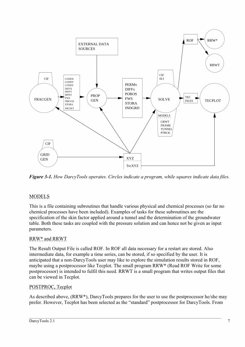
3.2 General structure DarcyTools is not one computer program, but a suite of “main codes” and a number of auxiliary ones. Figure 3-1 gives the relationship between the various components of DarcyTools. The figure also indicates the typical work process, as one normally “works from left to right in the diagram”. A first introduction to the various programs will now be given.
FRACGEN
This is the set of programs that generates material properties, i.e. conductivity, flow wetted surface, diffusivity and porosity fields, for the media. The name GEHYCO was first introduced for conductivity fields (GEnerate HYdraulic COnductivity). GEHYCO was later generalised to also calculate other property fields, but the name was kept. Perhaps it could be interpreted as GEnerate HYdraulic COnditions. The code that encapsulates the GEHYCO algorithm is called FRACGEN.
GRIDGEN
As the name indicates this is the program that generates the grid coordinates. Presently three types of grids can be used with DarcyTools: Cartesian, General Body-Fitted Coordinates (BFC) and a simplified version of BFC (BFC:s).
PROPGEN
This small auxiliary program is used to modify the properties generated by FRACGEN. This is useful if, as an example, the conductivity of the soil cover is to be established in a calibration process. The execution of FRACGEN may take hours in complex simulations, while PROPGEN will perform its task in a minute or two.
SOLVE
This is the program that solves the differential equations for pressure, salinity and other scalars. SOLVE hence contains subroutines for the formulation of the finite volume equations, boundary and source terms, etc. A key element in SOLVE is the solver of the linear equation system, MIGAL.
_____________________________________________________________________________________________ DarcyTools 2.1 7
FRACGENPROPGEN SOLVE TECPLOT
GRIDGEN XYZ
POROSFWSSTORAINDGRD
EXTERNAL DATASOURCES
ROF RRW*
CIFfif.f
TECFILES
CIF
MODELS
GRWTFRAMETUNNELPTRCK
RRWT
CIF
TecXYZ
FWSFREVOLSTORA
CONDYCONDX
CONDZ
DIFFYDIFFZ
DIFFX
FRCSET
PERMxDIFFx
Figure 3-1. How DarcyTools operates. Circles indicate a program, while squares indicate data files.
MODELS
This is a file containing subroutines that handle various physical and chemical processes (so far no chemical processes have been included). Examples of tasks for these subroutines are the specification of the skin factor applied around a tunnel and the determination of the groundwater table. Both these tasks are coupled with the pressure solution and can hence not be given as input parameters.
RRW* and RRWT
The Result Output File is called ROF. In ROF all data necessary for a restart are stored. Also intermediate data, for example a time series, can be stored, if so specified by the user. It is anticipated that a non-DarcyTools user may like to explore the simulation results stored in ROF, maybe using a postprocessor like Tecplot. The small program RRW* (Read ROF Write for some postprocessor) is intended to fulfil this need. RRWT is a small program that writes output files that can be viewed in Tecplot.
POSTPROC, Tecplot
As described above, (RRW*), DarcyTools prepares for the user to use the postprocessor he/she may prefer. However, Tecplot has been selected as the “standard” postprocessor for DarcyTools. From

_____________________________________________________________________________________________ DarcyTools 2.1 8
the input files a user can specify the content of Tecplot files, which are then generated by DarcyTools.
3.3 Mathematical Model DarcyTools computes fracture network flows using a continuum model in which the mass conservation equation is associated to several mass fraction transport equations for the salinity and/or particle mass concentrations, and to a heat transport equation. Conservation of mass:
( ) ( ) ( )u v w Qt x y zρθ ρ ρ ρ∂ ∂ ∂ ∂
+ + + =∂ ∂ ∂ ∂
(3-1)
where ρ is fluid density, θ porosity, u, v and w Darcy velocities and Q a source/sink term. The coordinate system is denoted x, y, z (space) and t (time).
Mass fraction transport equation:
x
y
z C
C CuC Dt x x
CvC Dy y
CwC D QC Qz z
ρθ ρ ργ
ρ ργ
ρ ργ
∂ ∂ ∂ + − ∂ ∂ ∂ ∂ ∂
+ − ∂ ∂ ∂ ∂ + − = + ∂ ∂
(3-2)
where C is transported mass fraction, xD , yD and zD the normal terms of the diffusion-dispersion tensor and cQ a source/sink term. When C is salinity, the source term represents the exchange with immobile zones and cQ is determined by the subgrid model FRAME. Note that the diffusion coefficients are the effective coefficients that include the porosity, see further explanation in connection with Equation (3-10) below.
Conservation of heat:
( )(1 )pp x
p y
p z p T
c c T Tuc Tt x x
Tvc Ty y
Twc T Q c T Qz z
ρθ θρ λ
ρ λ
ρ λ
∂ + − ∂ ∂ + − ∂ ∂ ∂ ∂ ∂
+ − ∂ ∂ ∂ ∂ + − = + ∂ ∂
(3-3)
where xλ , yλ and zλ are the normal terms of the equivalent (i.e. rock with fluid) thermal conductivity tensor, c is the rock thermal capacity and cp the specific heat of the fluid and TQ a
_____________________________________________________________________________________________ DarcyTools 2.1 9
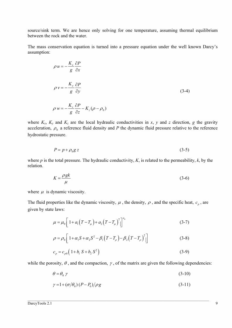
source/sink term. We are hence only solving for one temperature, assuming thermal equilibrium between the rock and the water. The mass conservation equation is turned into a pressure equation under the well known Darcy’s assumption:
0( )
x
y
zz
K Pug x
K Pvg y
K Pw Kg z
ρ
ρ
ρ ρ ρ
∂= −
∂
∂= −
∂
∂= − − −
∂
(3-4)
where Kx, Ky and Kz are the local hydraulic conductivities in x, y and z direction, g the gravity acceleration, 0ρ a reference fluid density and P the dynamic fluid pressure relative to the reference hydrostatic pressure.
0P p g zρ= + (3-5)
where p is the total pressure. The hydraulic conductivity, K, is related to the permeability, k, by the relation.
gkK ρµ
= (3-6)
where µ is dynamic viscosity.
The fluid properties like the dynamic viscosity, µ , the density, ρ , and the specific heat, pc , are given by state laws:
( ) ( )2
0 1 21n
a T T a T Tµ
µ µµ µ = + − + − (3-7)
( ) ( )220 1 2 1 21 S S T T T Tρ ρρ ρ α α β β = + + − − − −
(3-8)
( )20 1 21p pc c b S b S= + + (3-9)
while the porosity, θ , and the compaction, γ , of the matrix are given the following dependencies:
0θ θ γ= (3-10)
0 01 ( ) ( )P P gγ σ θ ρ= + − (3-11)

_____________________________________________________________________________________________ DarcyTools 2.1 10
In the above formulas S represents the salinity (salt mass fraction), 0θ a reference porosity field given for a reference pressure field P0 and σ the specific storativity field. nµ , ia , ib , iα , iβ , 0µ ,
0ρ , 0Cρ , Tµ and Tρ are constants.
In the advection/diffusion equation (3-2), it is common to write the diffusion coefficient as molDθ , where molD is the molecular diffusion coefficient. In DarcyTools we choose to write the term as
0mol molD D Dθ θ γ γ= = , where D is now the effective diffusion coefficient. The reason is that it is the effective diffusion coefficient that is specified for a conductive element and the GEHYCO-algorithm will hence deliver effective diffusion coefficients for cell walls. When a porous media case is simulated and the diffusion coefficients are specified, one thus needs to remember that it is the effective coefficients that should be given.
3.4 Finite volume equations and solver CFD (Computational Fluid Dynamics) methods transform the differential equations into algebraic ones, which can be solved by a computer and a computer program. DarcyTools uses the so-called finite volume method, which can be thought of as having three well-defined stages:
1) Discretize the computational domain into a number of cells, which fill entirely the domain.
2) Integrate each differential equation for each cell, to yield an algebraic equation.
3) Solve the resulting set of algebraic equations.
The differential equations were given in the previous section. After the integration, step 2 above, an algebraic equation of the following type results:
φSaaaaaaa TTBBNNSSEEWWPP +Φ+Φ+Φ+Φ+Φ+Φ=Φ (3-12)
where Φ denotes the variable in question, a coefficients and φS source terms. For further details see Report 1.
It is equations of type (3-12) that are solved by the solver MIGAL (see Report 1, Appendix A); in fact MIGAL can solve linked systems of this kind of equations, a feature that is used for the pressure-salinity coupling in the present set of equations.
3.5 Grid arrangements DarcyTools can only work with structured grids. Within this class, the following grids can be employed:
• BFC (Body Fitted Coordinates, sometimes called curvilinear grids). This is the most general type of grid. It is not generally used in practical applications, as it requires significant computer resources and a further limitation is that GEHYCO can not generate properties for this kind of grids.

_____________________________________________________________________________________________ DarcyTools 2.1 11
• BFC:s (BFC simplified). In this grid “all vertical lines remain vertical and the horizontal grid is cartesian, while the horizontal layers are allowed to float”. It is hence the grid to use to describe topography. This is the main grid used in DarcyTools for real world applications.
• Cartesian. In this grid, the grid coordinates can be specified as depending on only one coordinate, i.e. z (i, j, k) is only a function of k.
• Embedded grids. DarcyTools can employ embedded grids in several levels (see Report 1). Also mixed types, i.e. a Cartesian grid embedded in a BFC:s grid can be handled.
The four grid types are illustrated in Figure 3-2.
A further characterisation of the grid system concerns the variable locations. DarcyTools uses a so called node-centred arrangement, which means that variables (pressure, salinity, etc) are located at grid cell centres.

_____________________________________________________________________________________________ DarcyTools 2.1 12
Figure 3-2. The four grid types used in DarcyTools. Top-right grid only valid as a vertical section.
_____________________________________________________________________________________________ DarcyTools 2.1 13
3.6 Hardware, OS, etc DarcyTools is written in Fortran90, although some parts are restricted to Fortran77 (parts that non-DarcyTools user may need like the RRW* feature discussed above).
The following points give the currently favoured working environment:
• A PC/Workstation with as much power (processor, ram, disk space, graphics, etc) as possible.
• Red Hat LINUX, as operating system (8.0, 9,0 or enterprise 3.0)
• Intel Fortran Compiler 8.0 for LINUX
• Tecplot 10 for postprocessing
DarcyTools requires very little disk space (about 2MB), and calculations can be performed on a laptop. The concepts built into DarcyTools assume however a high resolution grid (more grid cells ⇒ more accurate simulation) and practical simulations can hence be quite demanding for the computer.
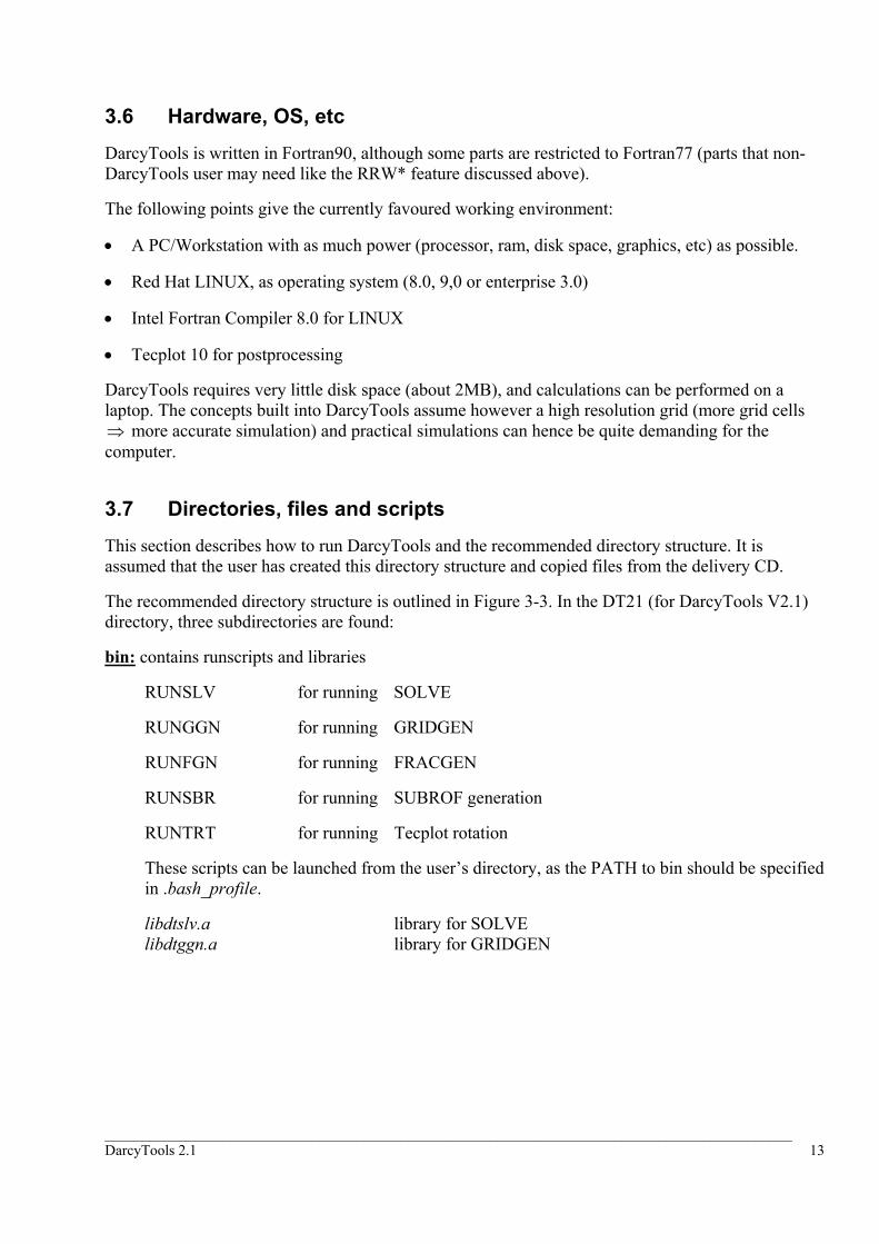
3.7 Directories, files and scripts This section describes how to run DarcyTools and the recommended directory structure. It is assumed that the user has created this directory structure and copied files from the delivery CD.
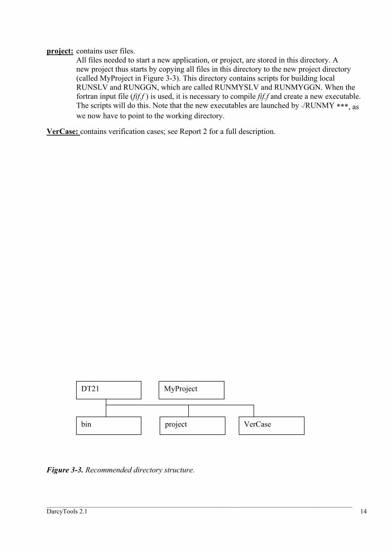
The recommended directory structure is outlined in Figure 3-3. In the DT21 (for DarcyTools V2.1) directory, three subdirectories are found:
bin: contains runscripts and libraries
RUNSLV for running SOLVE
RUNGGN for running GRIDGEN
RUNFGN for running FRACGEN
RUNSBR for running SUBROF generation
RUNTRT for running Tecplot rotation
These scripts can be launched from the user’s directory, as the PATH to bin should be specified in .bash_profile.
libdtslv.a library for SOLVE libdtggn.a library for GRIDGEN
_____________________________________________________________________________________________ DarcyTools 2.1 14
project: contains user files. All files needed to start a new application, or project, are stored in this directory. A new project thus starts by copying all files in this directory to the new project directory (called MyProject in Figure 3-3). This directory contains scripts for building local RUNSLV and RUNGGN, which are called RUNMYSLV and RUNMYGGN. When the fortran input file (fif.f ) is used, it is necessary to compile fif.f and create a new executable. The scripts will do this. Note that the new executables are launched by ·/RUNMY ***, as we now have to point to the working directory.
VerCase: contains verification cases; see Report 2 for a full description.
Figure 3-3. Recommended directory structure.
DT21 MyProject
bin project VerCase

_____________________________________________________________________________________________ DarcyTools 2.1 15
4 Compact Input File (CIF) 4.1 Introduction The main input specification to DarcyTools is by way of a Compact Input File (CIF). The CIF is a free formatted file that contains both comment and command lines. The comment lines are defined as being any empty line or a line whose first character is the ‘*’ or ‘c’ character. The command lines are defined as being all other lines. Each command line starts with an integer value representing the command identification number. The data follow this integer ID according to the specified format of the command.
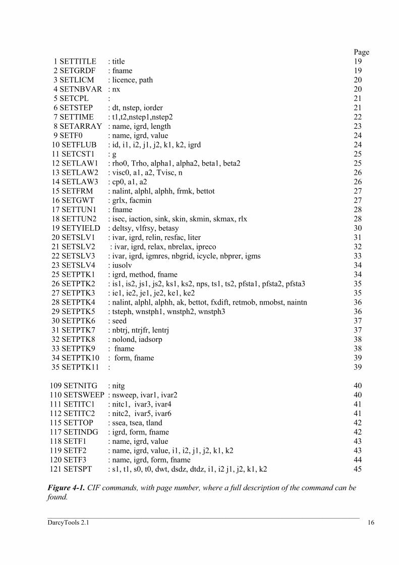
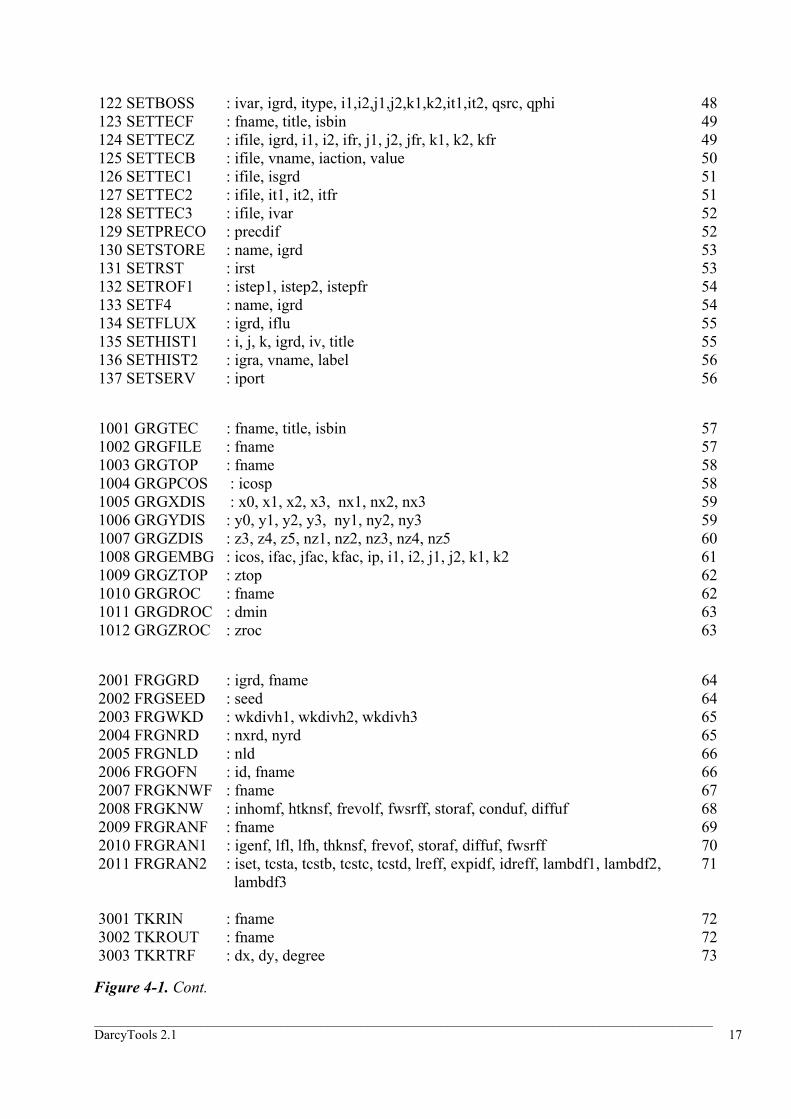
A list of all CIF commands is given in Figure 4-1. The page number, where a full description of the command is found, is also provided.
The group of commands, 1 to 99, corresponds to commands that affect the memory allocation, the F-array, while commands starting from 100 have to be called after the F array allocation. Commands for special tasks (GRIDGEN, FRACGEN, TECROT and SUBROF) have their individual command group numbers, as can be seen in Figure 4-1.
Further information related to the CIF commands can be found in the Notation, Section 9, and examples of use are given by the thirty verification cases. Four of these cases are listed in Appendix C.
In the following all CIF commands will be described, in the order as they appear in the CIF. After the command line a line with data statements will follow. The only purpose of this line is to illustrate the command; the actual numbers have no significance.
_____________________________________________________________________________________________ DarcyTools 2.1 16
Page 1 SETTITLE : title 19 2 SETGRDF : fname 19 3 SETLICM : licence, path 20 4 SETNBVAR : nx 20 5 SETCPL : 21 6 SETSTEP : dt, nstep, iorder 21 7 SETTIME : t1,t2,nstep1,nstep2 22 8 SETARRAY : name, igrd, length 23 9 SETF0 : name, igrd, value 24 10 SETFLUB : id, i1, i2, j1, j2, k1, k2, igrd 24 11 SETCST1 : g 25 12 SETLAW1 : rho0, Trho, alpha1, alpha2, beta1, beta2 25 13 SETLAW2 : visc0, a1, a2, Tvisc, n 26 14 SETLAW3 : cp0, a1, a2 26 15 SETFRM : nalint, alphl, alphh, frmk, bettot 27 16 SETGWT : grlx, facmin 27 17 SETTUN1 : fname 28 18 SETTUN2 : isec, iaction, sink, skin, skmin, skmax, rlx 28 19 SETYIELD : deltsy, vlfrsy, betasy 30 20 SETSLV1 : ivar, igrd, relin, resfac, liter 31 21 SETSLV2 : ivar, igrd, relax, nbrelax, ipreco 32 22 SETSLV3 : ivar, igrd, igmres, nbgrid, icycle, nbprer, igms 33 23 SETSLV4 : iusolv 34 25 SETPTK1 : igrd, method, fname 34 26 SETPTK2 : is1, is2, js1, js2, ks1, ks2, nps, ts1, ts2, pfsta1, pfsta2, pfsta3 35 27 SETPTK3 : ie1, ie2, je1, je2, ke1, ke2 35 28 SETPTK4 : nalint, alphl, alphh, ak, bettot, fxdift, retmob, nmobst, naintn 36 29 SETPTK5 : tsteph, wnstph1, wnstph2, wnstph3 36 30 SETPTK6 : seed 37 31 SETPTK7 : nbtrj, ntrjfr, lentrj 37 32 SETPTK8 : nolond, iadsorp 38 33 SETPTK9 : fname 38 34 SETPTK10 : form, fname 39 35 SETPTK11 : 39 109 SETNITG : nitg 40 110 SETSWEEP : nsweep, ivar1, ivar2 40 111 SETITC1 : nitc1, ivar3, ivar4 41 112 SETITC2 : nitc2, ivar5, ivar6 41 115 SETTOP : ssea, tsea, tland 42 117 SETINDG : igrd, form, fname 42 118 SETF1 : name, igrd, value 43 119 SETF2 : name, igrd, value, i1, i2, j1, j2, k1, k2 43 120 SETF3 : name, igrd, form, fname 44 121 SETSPT : s1, t1, s0, t0, dwt, dsdz, dtdz, i1, i2 j1, j2, k1, k2 45 Figure 4-1. CIF commands, with page number, where a full description of the command can be found.
_____________________________________________________________________________________________ DarcyTools 2.1 17
122 SETBOSS : ivar, igrd, itype, i1,i2,j1,j2,k1,k2,it1,it2, qsrc, qphi 48 123 SETTECF : fname, title, isbin 49 124 SETTECZ : ifile, igrd, i1, i2, ifr, j1, j2, jfr, k1, k2, kfr 49 125 SETTECB : ifile, vname, iaction, value 50 126 SETTEC1 : ifile, isgrd 51 127 SETTEC2 : ifile, it1, it2, itfr 51 128 SETTEC3 : ifile, ivar 52 129 SETPRECO : precdif 52 130 SETSTORE : name, igrd 53 131 SETRST : irst 53 132 SETROF1 : istep1, istep2, istepfr 54 133 SETF4 : name, igrd 54 134 SETFLUX : igrd, iflu 55 135 SETHIST1 : i, j, k, igrd, iv, title 55 136 SETHIST2 : igra, vname, label 56 137 SETSERV : iport 56
1001 GRGTEC : fname, title, isbin 57 1002 GRGFILE : fname 57 1003 GRGTOP : fname 58 1004 GRGPCOS : icosp 58 1005 GRGXDIS : x0, x1, x2, x3, nx1, nx2, nx3 59 1006 GRGYDIS : y0, y1, y2, y3, ny1, ny2, ny3 59 1007 GRGZDIS : z3, z4, z5, nz1, nz2, nz3, nz4, nz5 60 1008 GRGEMBG : icos, ifac, jfac, kfac, ip, i1, i2, j1, j2, k1, k2 61 1009 GRGZTOP : ztop 62 1010 GRGROC : fname 62 1011 GRGDROC : dmin 63 1012 GRGZROC : zroc 63
2001 FRGGRD : igrd, fname 64 2002 FRGSEED : seed 64 2003 FRGWKD : wkdivh1, wkdivh2, wkdivh3 65 2004 FRGNRD : nxrd, nyrd 65 2005 FRGNLD : nld 66 2006 FRGOFN : id, fname 66 2007 FRGKNWF : fname 67 2008 FRGKNW : inhomf, htknsf, frevolf, fwsrff, storaf, conduf, diffuf 68 2009 FRGRANF : fname 69 2010 FRGRAN1 : igenf, lfl, lfh, thknsf, frevof, storaf, diffuf, fwsrff 70 2011 FRGRAN2 : iset, tcsta, tcstb, tcstc, tcstd, lreff, expidf, idreff, lambdf1, lambdf2, 71 lambdf3 3001 TKRIN : fname 72 3002 TKROUT : fname 72 3003 TKRTRF : dx, dy, degree 73
Figure 4-1. Cont.

_____________________________________________________________________________________________ DarcyTools 2.1 18
4000 SBRTITLE : title 73 4001 SBRGIN : fname 74 4002 SBRGOUT : fname 74 4003 SBRRIN : fname 75 4004 SBRROUT : fname 75 4005 SBRPDEF : icos, ifac, jfac, kfac, ip, i1, i2, j1, j2, k1, k2 76 4006 SBRTEC : fname, title, isbin 76
Figure 4-1. Cont.

_____________________________________________________________________________________________ DarcyTools 2.1 19
4.2 Commands
1 SETTITLE __________________________________________________________________
* 1 SETTITLE : title
1 'Taylor Dispersion'
This command defines a title for the current run. The title will appear on the Monitor screen and in various output files.
The title string must be less than 256 characters long. The default string is an empty string.
2 SETGRDF __________________________________________________________________
* 2 SETGRDF : fname
2 'xyz'
The grid is specified in the unformatted file 'xyz', where xyz is a user chosen name that may be up to 256 characters long.
The default grid is a Cartesian grid with 10=== nknjni and 1=== dzdydx .
Usually the file is generated by a set of CIF commands, see commands starting with number 1001, perhaps reading in a topography file.

_____________________________________________________________________________________________ DarcyTools 2.1 20
3 SETLICM __________________________________________________________________
* 3 SETLICM : licence, path
3 'bx / yXz ' ‘ ‘
This command sets the unlocking string for the MIGAL solver. When MIGAL is protected by a software license manager the path defining the license log-file must also be set. When MIGAL is protected by a hardware key (dongle) the path name must be an empty string.
4 SETNBVAR __________________________________________________________________
* 4 SETNBVAR: nx
4 3
This command fixes the number of variables contained in the X sub-array. The default value is 3 since the salinity and the temperature are always used to compute the fluid properties. In case of fixed properties, the salinity and the temperature will be present in X sub-array but not solved for. In the same way, when computing transport of a scalar quantity only, the pressure must be stored to define the mass fluxes. Hence, the first variable of the X sub-array will always be the pressure, the second variable the salinity and the third variable the temperature. Users should note that, when the pressure or the salinity or the temperature is fixed, they have the opportunity not to solve them by setting adequate loop indexes via SETSWEEP, SETITC1 and SETITC2.

_____________________________________________________________________________________________ DarcyTools 2.1 21
5 SETCPL __________________________________________________________________
* 5 SETCPL :
5
This command switches ON a coupled solution for the pressure and salinity variables. Since the default setting is the segregated algorithm this routine has to be called only when the coupled solution is desired. The command has no dummy arguments. When switched ON, the coupled solution is set for every grid of the domain.
6 SETSTEP __________________________________________________________________
* 6 SETSTEP : dt, nstep, iorder
6 10. 100 1
This command defines the time integration loop as well as an initial time step. It also set the default ROF output control parameters and should be called before SETROF1. The default values are those of a stationary case: 1, 0nstep iorder= = and dt not used. iorder = 1 gives a Euler first order implicit scheme while iorder = 2 gives a second order scheme, see Report 1. A variable dt can also be specified; see command 7 SETTIME

_____________________________________________________________________________________________ DarcyTools 2.1 22
7 SETTIME __________________________________________________________________
* 7 SETTIME : t1, t2, nstep1, nstep2
7 10. 20. 10 20
A variable time step can be specified with this command. This command should be considered together with SETSTEP, as information in both specifies the time step distribution. nstep1 nstep 2 nstep3
0 t1 t2 t3
where: nstep3 = nstep – nstep1 – nstep2
t3 = t2 + dt × nstep3
The tree parts give a uniform, expanding/contracting (hyperbolic tangent distribution) and uniform time step.
The default values are t1 = t2 = 0 and nstep1 = nstep2 = 0, which means that the specification in SETSTEP governs the distribution.
_____________________________________________________________________________________________ DarcyTools 2.1 23
8 SETARRAY __________________________________________________________________
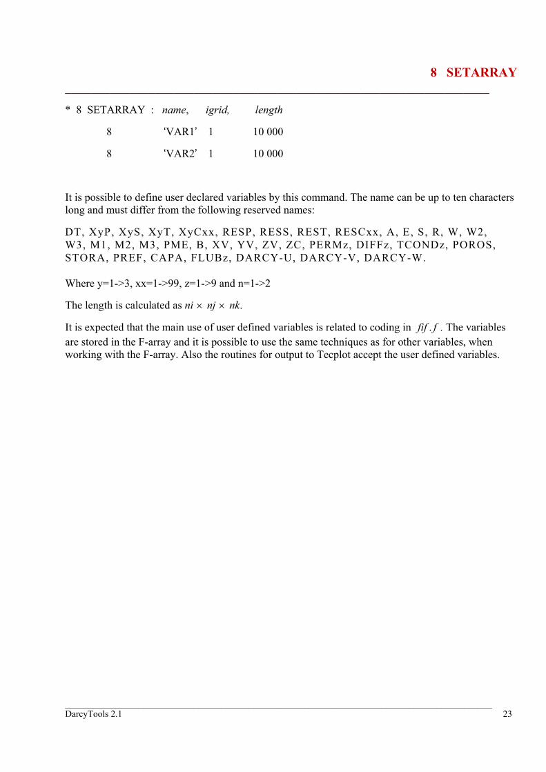
* 8 SETARRAY : name, igrid, length
8 ‘VAR1’ 1 10 000
8 ‘VAR2’ 1 10 000
It is possible to define user declared variables by this command. The name can be up to ten characters long and must differ from the following reserved names:
DT, XyP, XyS, XyT, XyCxx, RESP, RESS, REST, RESCxx, A, E, S, R, W, W2, W3, M1, M2, M3, PME, B, XV, YV, ZV, ZC, PERMz, DIFFz, TCONDz, POROS, STORA, PREF, CAPA, FLUBz, DARCY-U, DARCY-V, DARCY-W. Where y=1->3, xx=1->99, z=1->9 and n=1->2
The length is calculated as ni × nj × nk.
It is expected that the main use of user defined variables is related to coding in ffif . . The variables are stored in the F-array and it is possible to use the same techniques as for other variables, when working with the F-array. Also the routines for output to Tecplot accept the user defined variables.

_____________________________________________________________________________________________ DarcyTools 2.1 24
9 SETF0 __________________________________________________________________
* 9 SETF0 : vname, igrid, val
9 ‘POROS‘ 1 1.E - 3
9 ‘PERM3‘ 1 1.E - 9
This command declares the array named ‘vname’ as being 1 element long on the given grid igrd and fills its unique value with val. This facility allows memory saving when a property is uniform in the whole domain. It applies only to the following arrays: POROS, STORA, PREF, CAPA, TCONDx, PERMx and DIFFx with x=1…9.
See also commands 118 → 120, which give alternative ways of array specification.
10 SETFLUB __________________________________________________________________
* 10 SETFLUB : id, i1, i2, j1, j2, k1, k2, igrid
10 4 10 20 10 30 5 15 2
This command declares the array named FLUBid as being 1 element long (instead of 0) and set the footprint command for the flux balance definition on the given grid igrid. id should remain between 0 and 9. When no footprint index is null FLUBid contains the mass fluxes balance on the given footprint. When one index is null (e.g. j2) FLUBid contains the mass fluxes sum through the footprint of the corresponding plane (j=j1). The fluxes are then east, north or top fluxes of the cells (i,j1,k). Only one index may be null at a time. When no index is null the footprint index can vary from 2 to nbcells-1. When one index is null the corresponding footprint index can vary from 1 to nbcells-1 (nj-1) and the other indexes from 1 to nbcells.
The mass flux balance is usually used for convergence monitoring. It may also be useful if the flux through the domain, in a certain direction, is of interest.

_____________________________________________________________________________________________ DarcyTools 2.1 25
11 SETCST1 __________________________________________________________________
* 11 SETCST1 : g
11 9.81
The default value of the acceleration of gravity is 9.81 and this command does not normally need to be set. It may be used if a problem is scaled in some way or if gravitational forces are not considered. However, for the latter case command 12 SETLAW1 is often used.
12 SETLAW1 __________________________________________________________________
* 12 SETLAW1 : rho0, Trho, alpha1, alpha2, beta1, beta2
12 1000. 0.0 0.008 0.0 0.0 0.0
This command sets the density state law parameters. The default values are:
0
0
1
2
1
2
1000.0.00.0080.00.00.0
rTaabb
======
They represent the constants of the following law: ( )2 2
0 1 2 1 0 2 01 ( ) ( )r a S a S b T T b T Tρ = + + − − − −
For complex situations, with non-linear and coupled relations, it is left to the user to specify the constants that fit the problem best.
_____________________________________________________________________________________________ DarcyTools 2.1 26
13 SETLAW2 __________________________________________________________________
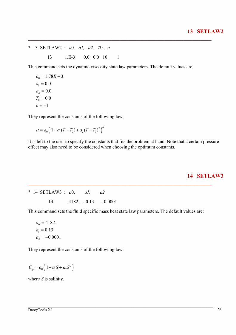
* 13 SETLAW2 : a0, a1, a2, T0, n
13 1.E-3 0.0 0.0 10. 1
This command sets the dynamic viscosity state law parameters. The default values are:
0
1
2
0
1.78 30.00.00.01
a EaaTn
= −==== −
They represent the constants of the following law:
( )20 1 0 2 01 ( ) ( )
na a T T a T Tµ = + − + −
It is left to the user to specify the constants that fits the problem at hand. Note that a certain pressure effect may also need to be considered when choosing the optimum constants.
14 SETLAW3 __________________________________________________________________
* 14 SETLAW3 : a0, a1, a2
14 4182. - 0.13 - 0.0001
This command sets the fluid specific mass heat state law parameters. The default values are:
0
1
2
4182.0.13
0.0001
aaa
=== −
They represent the constants of the following law:
( )20 1 21pC a a S a S= + +
where S is salinity.

_____________________________________________________________________________________________ DarcyTools 2.1 27
15 SETFRM __________________________________________________________________
* 15 SETFRM : nalint, alph1, alph2, frmk, bettot
15 10 1.E-8 1.E-3 2.0 10.
This command activates the subgrid model FRAME, as applied to the salinity equation. The meaning of the variables are
nalint = number of alpha intervals.
alph1 = low alpha limit.
alph2 = high alpha limit.
=frmk FRAME – k, where k is late time slope of a breakthrough curve.
=bettot global value of volume ratio (immobile/mobile)
The reader is referenced to Report 1 for a background to this model and its parameters.
16 SETGRWT __________________________________________________________________
* 16 SETGRWT : grlx, facmin
16 0.2 1.E - 3
This command activates the Ground Water Table calculation. The two parameters are:
grlx = under relaxation parameter.
facmin = minimum property reduction factor.
See Report 1 for further background.

_____________________________________________________________________________________________ DarcyTools 2.1 28
17 SETTUN1 __________________________________________________________________
* 17 SETTUN1 : fname
17 ‘tunfile’
This command activates the TUNNEL model and reads the tunnel section definitions in the file named ‘fname’.
The file should be a formatted file, giving the location of the tunnel sections in grid space. Each tunnel cell should hence be listed and it should further be specified which grid and tunnel section it belongs to.
Format:
nbcells
i j k igrd isection
Where nbcells is the number of tunnel cells (hence the number of lines to follow).
Note also that all tunnel cells should be specified in the INDGRD-array. See the Demo Case (Section 7) for an example.
_____________________________________________________________________________________________ DarcyTools 2.1 29
18 SETTUN2 __________________________________________________________________
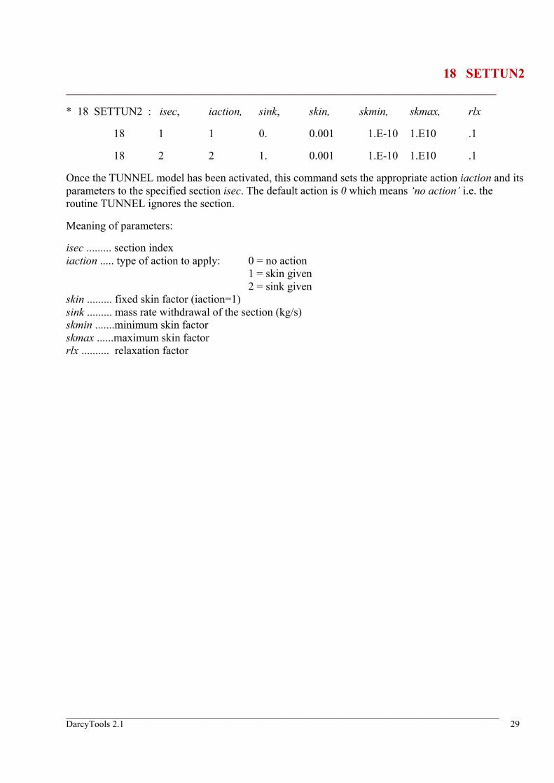
* 18 SETTUN2 : isec, iaction, sink, skin, skmin, skmax, rlx
18 1 1 0. 0.001 1.E-10 1.E10 .1
18 2 2 1. 0.001 1.E-10 1.E10 .1
Once the TUNNEL model has been activated, this command sets the appropriate action iaction and its parameters to the specified section isec. The default action is 0 which means ‘no action’ i.e. the routine TUNNEL ignores the section.
Meaning of parameters:
isec ......... section index iaction ..... type of action to apply: 0 = no action 1 = skin given 2 = sink given skin ......... fixed skin factor (iaction=1) sink ......... mass rate withdrawal of the section (kg/s) skmin .......minimum skin factor skmax ......maximum skin factor rlx .......... relaxation factor

_____________________________________________________________________________________________ DarcyTools 2.1 30
19 SETYIELD __________________________________________________________________
* 19 SETYIELD : deltsy, vlfrsy, betasy
19 50. 0.2 0.0
Once the Ground Water Table model has been activated, this routine sets the appropriate specific yield parameters and creates the GWT_VSY sub-array. The default values correspond to zero specific yield.
Meaning of parameters:
deltsy ....... time constant for delayed response vlfrsy ....... volume fraction that contains the yield water betasy .......immobile to mobile volume fraction
Note that two alternative ways of specifying the specific yield volume are supported. Only one can be active; the other should be given a value of 0.0.
See Report 1 for details.

_____________________________________________________________________________________________ DarcyTools 2.1 31
20 SETSLV1 __________________________________________________________________
* 20 SETSLV1 : ivar, igrd, relin, resfac, liter
20 2 1 1. 0.1 2
This command defines for each grid and each variable to solve, the first level of the MIGAL solver parameters. When setting a null index for the grid or the variable, the parameters are set to all the grids or all the variables respectively. When a coupled solution is performed, only the salinity values are taken into account for the pressure-salinity couple. These parameters are in relation with the quality of the solution to perform during a sweep. RELIN is the relaxation parameter applied to the solution from one sweep to the next one. RESFAC fixes the residual reduction level which stops MIGAL, and LITER fixes the maximum number of sweeps allowed when RESFAC is not reached. Defaults values are:
relin = 1.
resfac = 0.1
liter = 2
Meaning of parameters:
ivar ......... index of variable igrd ......... index of grid relin ........ relaxation parameter of final MIGAL's solution resfac ...... ending condition: stop when RMS residuals are reduced by the factor resfac liter ........ maximum number of cycles allowed

_____________________________________________________________________________________________ DarcyTools 2.1 32
21 SETSLV2 __________________________________________________________________
* 21 SETSLV2 : ivar, igrd, relax, nbrelax, ipreco
21 0 0 .95 3 1
This command defines for each grid and each variable to solve, the second level of the MIGAL solver parameters. When setting a null index for the grid or the variable, the parameters are set to all the grids or all the variables respectively. When a coupled solution is performed, only the salinity values are taken into account for the pressure-salinity couple. These parameters are in relation with the effort imposed to the MIGAL smoother in order to reduce the residuals during iterations (cycles). RELAX fixes the relaxation parameter of the ILU smoother, NBRELAX fixes the number of post-prolongation relaxations and IPRECO the number of multi-grid cycles preconditioning the GMRES iterations. Defaults values are:
relax = .95
nbrelax = 3
ipreco = 1
Meaning of parameters:
ivar ......... index of variable igrd ......... index of grid relax ........ relaxation parameter for multi-grid smoother nbrelax .... number of relaxation for each smoother run ipreco ...... number of multi-grid cycles for each gmres iteration
_____________________________________________________________________________________________ DarcyTools 2.1 33
22 SETSLV3 __________________________________________________________________
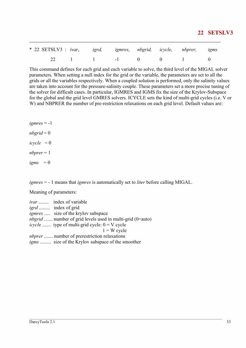
* 22 SETSLV3 : ivar, igrd, igmres, nbgrid, icycle, nbprer, igms
22 1 1 -1 0 0 1 0
This command defines for each grid and each variable to solve, the third level of the MIGAL solver parameters. When setting a null index for the grid or the variable, the parameters are set to all the grids or all the variables respectively. When a coupled solution is performed, only the salinity values are taken into account for the pressure-salinity couple. These parameters set a more precise tuning of the solver for difficult cases. In particular, IGMRES and IGMS fix the size of the Krylov-Subspace for the global and the grid level GMRES solvers. ICYCLE sets the kind of multi-grid cycles (i.e. V or W) and NBPRER the number of pre-restriction relaxations on each grid level. Default values are:
igmres = -1
nbgrid = 0
icycle = 0
nbprer = 1
igms = 0
igmres = - 1 means that igmres is automatically set to liter before calling MIGAL.
Meaning of parameters:
ivar ........ index of variable igrd ......... index of grid igmres ..... size of the krylov subspace nbgrid ....... number of grid levels used in multi-grid (0=auto) icycle ....... type of multi-grid cycle: 0 = V cycle 1 = W cycle nbprer ....... number of prerestriction relaxations igms ......... size of the Krylov subspace of the smoother
_____________________________________________________________________________________________ DarcyTools 2.1 34
23 SETSLV4 __________________________________________________________________
* 23 SETSLV4 : ivar, igrd, iusolv
23 0 0 6
This command defines for each grid and each variable to solve, the output file for the residuals printings. When setting a null index for the grid or the variable, the parameters are set to all the grids or all the variables respectively. When a coupled solution is performed, only the salinity values are taken into account for the pressure-salinity couple. Defaults value is:
iusolv = 6
Meaning of parameters:
ivar ......... index of variable igrd ......... index of grid iusolv ....... MIGAL output unit ( 0 = no output) (-1 = solve.log) ( 6 = screen )
25 SETPTK1 __________________________________________________________________
* 25 SETPTK1 : igrd, method, fname
25 1 2 ‘ ‘
This command sets the PARTRACK method parameters for the given grid. It is this routine that switches ON the PARTRACK feature. When a restart is made a valid file name must be set in fname. Hence, during the last time step, the particles positions and states will be saved. Then the file fname will have to be specified again for proceeding to the restart of PARTRACK. Nevertheless it is also possible to start or suspend PARTRACK for the restart computations.
Meaning of parameters:
igrd ......... index of grid method ....... PARTRACK method (1 or 2) fname ........ PARTRACK restart file name

_____________________________________________________________________________________________ DarcyTools 2.1 35
26 SETPTK2 __________________________________________________________________
* 26 SETPTK2 : is1, is2, js1, js2, ks1, ks2, nps, ts1, ts2, pfstal, pfsta2, pfsta3
26 1 2 10 20 5 10 100 0. 0. 0.5 0.5 0.5
This command sets the footprint in which the PARTRACK particles are initially spread out. Since the footprint refers to the PARTRACK grid the routine SETPTK1 must have been called before. The particles are spread out along the unrolled index array of the footprint.
Meaning of parameters:
is1, is2 ...... span of the starting footprint in x-direction js1, js2 ...... span of the starting footprint in y-direction ks1, ks2 ..... span of the starting footprint in z-direction ts1, ts2 ...... span of the starting footprint in time-direction nps ............ number of particles pfsta1 ....... initial relative x position in cells [0,1] pfsta2 ....... initial relative y position in cells [0,1] pfsta3 ....... initial relative z position in cells [0,1]
27 SETPTK3 __________________________________________________________________
* 27 SETPTK3 : ie1, ie2, je1, je2, ke1, ke2
27 25 25 50 50 40 40
This command sets the footprint in which the PARTRACK particles are captured. Since the footprint refers to the PARTRACK grid the routine SETPTK1 must have been called before. The particles arriving in this footprint are removed and counted in the variable PTK_NPC while the number of particles leaving through the grid boundary is given by (PTK_NPO - PTK_NPC). The default values are ie1=ie2=je1=je2=ke1=ke2=0 and disable the capturing feature.
Meaning of parameters:
ie1, ie2 ...... span of the arriving footprint in x-direction je1, je2 ...... span of the arriving footprint in y-direction ke1, ke2 .....span of the arriving footprint in z-direction

_____________________________________________________________________________________________ DarcyTools 2.1 36
28 SETPTK4 __________________________________________________________________
* 28 SETPTK4 : nalint, alphl, alphh, ak, bettot, fxdift, retmob, nmobst, naintn
28 100 1.E-9 1.E-3 2.0 10. 1.E-5 1.5 5 100
This routine sets the PARTRACK multi-rate model parameters. The default values disable this model.
Meaning of parameters:
nalint ....... number of alpha intervals (= naintt) alphl ........ low aplha limit alphh ....... high aplha limit ak ............ late time slope of breakthrough curve bettot ....... global value of volume ratio (immobile/mobile) fxdift ....... uniform cross diffusion coefficient retmob ..... retardation mobile nmobst ..... number of a/d states in the mobile zone naintn ...... number of a/d states in the immobile zone
The reader is referred to Report 1 for further details and a general background.
29 SETPTK5 __________________________________________________________________
* 29 SETPTK5 : tsteph, wnstph1, wnstph2, wnstph3
29 1. 0.1 0.1 0.1
This command sets the PARTRACK parameters when the first method is specified (method=1 in SETPTK1). The default values are:
tsteph = 10.
wnstph1 = wnstph2 = wnstph3 = 0.1
Meaning of parameters:
tsteph ....... velocity freezing time [s] wnstph1 ...... x displacement limit for velocity freezing wnstph2 ...... y displacement limit for velocity freezing wnstph3 ...... z displacement limit for velocity freezing
_____________________________________________________________________________________________ DarcyTools 2.1 37
30 SETPTK6 __________________________________________________________________
* 30 SETPTK6 : seed
30 0.4391
This command sets the PARTRACK random generator initialisation seed. By default this parameter is set from the clock time of the computer (i.e. seconds and milliseconds).
31 SETPTK7 __________________________________________________________________
* 31 SETPTK7 : nbtrj, ntrjfr, lentrj,
31 100 1 1000
This command sets the number of PARTRACK trajectories and their time definition in terms of time step frequency and maximum length. When the number of trajectories is less than the total number of particles, the selected particles are spread out in the particles array. Hence, during a restart, the total number of particles and trajectories must remain identical. The trajectories are stored in the F sub-arrays named PTK_TRJX, PTK_TRJY, PTK_TRJZ and PTK_TRJT. In the same way that the density of particles PTK_DEN, the trajectories can be outputted in a TECPLOT file by using SETTECB with the name PTK_TRJ. Nevertheless, it is recommended to output the trajectories in a devoted TECPLOT file. The trajectories are saved in the PARTRACK restart file when this file has been specified in SETPTK1. By default no trajectories are produced.
Meaning of parameters:
nbtrj ........ number of trajectories ntrjfr ....... time step frequency for trajectory outputs lentrj ....... lentgh of trajectories in time steps
_____________________________________________________________________________________________ DarcyTools 2.1 38
32 SETPTK8 __________________________________________________________________
* 32 SETPTK8 : nolond, iadsorp
32 1 0
This command sets the PARTRACK longitudinal diffusion and adsorption triggers. The default values are:
nolond = 1
iadsorp = 0
Meaning of parameters:
nolond ....... longitudinal diffusion (1=no, 0=yes) iadsorp ...... adsorption (1=yes, 0=no)
See Report 1 for details about nolond.
33 SETPTK9 __________________________________________________________________
* 33 SETPTK9 : fname
33 ‘pdata’
This command specifies the filename of a file where startpositions of particles are given. The format of the data is the same as for command 26. However, the first line of the file should specify the number of specifications that follow, i e the number of lines.

_____________________________________________________________________________________________ DarcyTools 2.1 39
34 SETPTK10 __________________________________________________________________
* 34 SETPTK10 : form, fname
34 ‘unformatted’ ‘fquo.dat’
This command activates the F-quotient calculation and also specify the name and form of the result file. Note that only method = 1 is allowed for calculation of F-quotients. When the unformatted option is used, which may be advisable for large files, a small code is required to read the file and perfom required further development of the results (for example statistics).
35 SETPTK11 __________________________________________________________________
* 35 SETPTK11 :
35
The free volume in each cell, required by PARTRACK, is by default calculated from the porosity field. This command activates an alternative specification by the array PTK_FREVOL, where the free volume in each cell is given.
_____________________________________________________________________________________________ DarcyTools 2.1 40
109 SETNITG __________________________________________________________________
* 109 SETNITG : nitg
109 5
This command defines the number of iterations that the program must accomplish during each time step to solve the interaction between the different grid solutions. The default value is:
nitg = 1
110 SETSWEEP __________________________________________________________________
* 110 SETSWEEP : nsweep, ivar1, ivar2
110 10 1 3
This command defines the number of sweeps to perform per time step, on each grid. It also defines the variables to solve in this iteration loop. Defaults values are:
nsweep = ivar1 = ivar2 = 1
Meaning of parameters:
nsweep ...... number of coupling iterations ivar1 ...... lower limit of the loop on variables ivar2 ....... upper limit of the loop on variables

_____________________________________________________________________________________________ DarcyTools 2.1 41
111 SETITC1 __________________________________________________________________
* 111 SETITC1 : nitc1, ivar3, ivar4
111 2 3 3
This command defines the number of iterations to perform per time step, on each grid for coupling the variables ivar3 to ivar4 inside the sweep loop. Defaults values are:
nitc1 = 0
ivar3 = 0
ivar4 = 0
Meaning of parameters:
nitc1 ...... number of coupling iterations ivar3 .... lower limit of the loop on variables ivar4 ..... upper limit of the loop on variables
112 SETITC2 __________________________________________________________________
* 112 SETITC2 : nitc2, ivar5, ivar6
112 2 4 4
This command defines the second number of iterations to perform per time step, on each grid for coupling the variables ivar5 to ivar6 outside the sweep loop. Defaults values are:
nitc2 = 0
ivar5 = 0
ivar6 = 0
Meaning of parameters:
nitc2 ...... number of coupling iterations ivar5 .... lower limit of the loop on variables ivar6 ..... upper limit of the loop on variables

_____________________________________________________________________________________________ DarcyTools 2.1 42
115 SETTOP __________________________________________________________________
* 115 SETTOP : ssea, tsea, tland
115 1.0 5. 10.
This command sets the the top boundary conditions (k=nk). The top boundary is considered as being land where z(nk+1)>0 or PME(i,j) differs from zero. Elsewhere the top boundary is considered as being sea bottom. PME is an array containing the precipitation minus the evaporation velocity, which can be set using the routines SETF1, SETF2 or SETF3. Besides adding the PME mass source term, the command fixes in k=nk the salinity to zero on land and ssea on sea bottom, the temperature to tland on land and to tsea on sea bottom and the pressure to:
( )( ),( ) 0 sea seasea c nk S TP z g ρ ρ= −
Meaning of parameters:
ssea ......... salinity of the sea (z<0) tsea ......... temperature of the sea (z<0) tland ........ temperature of the land (z>0)
117 SETINDG __________________________________________________________________
* 117 SETINDG : igrd, form, fname,
117 1 ‘FORMATTED’ ‘INDFILE’
This command fills the INDGRD array associated with the grid igrd with the values read in the file fname. When form=’FORMATTED’ the file must be formatted but is read with free format. Any line starting with the character ‘*’ is then considered as being a comment line. The values are read by the following statements:
Formatted files: read(iu,*) (indgrd(i),i=1,ni*nj*nk)
Unformatted files: read(iu) (indgrd(i),i=1,ni*nj*nk)
Where ni, nj and nk are the dimensions of the given grid.
Meaning of parameters:
igrd ......... index of the grid form .........form specifier of the file to open fname .......name of the file containing the values

_____________________________________________________________________________________________ DarcyTools 2.1 43
118 SETF1 __________________________________________________________________
* 118 SETF1 : vname, igrd, val
118 ‘X1P’ 2 1.E4
This command fills the entire sub-array named vname on the grid igrd with the value val.
119 SETF2 __________________________________________________________________
* 119 SETF2 : vname, igrd, val, i1, i2, j1, j2, k1, k2
119 ‘X1S’ 1 0.5 10 20 1 50 1 20
This command sets the value val into the specified footprint of the sub-array named vname on the grid igrd. The dimension of the given sub-array must be (ni,nj,nk) if the associated grid has nknjni ×× cells. Nevertheless when i1 or i2 etc equals zero the corresponding dimension is discarded. For example, filling a 2D (ni,nk) array can be achieved by setting j1 = j2 = 0.
Meaning of parameters:
vname ........ name of the variable igrd ......... index of the grid val .......... value to set in the footprint i1, i2 ........ setting's footprint x-definition j1, j2 ........ setting's footprint y-definition k1, k2 ........ setting's footprint z-definition

_____________________________________________________________________________________________ DarcyTools 2.1 44
120 SETF3 __________________________________________________________________
* 120 SETF3 : vname, igrd, form, fname
120 ‘X2P’ 1 ‘UNFORMATTED’ ‘PINIVAL’
This command fills the entire sub-array named vname on the grid igrd with the values read in the file named fname. When the form of the file is specified as being the string ‘FORMATTED’, the file is read without any predefined format. Further, any line starting with the character ‘*’ is considered to be a comment line as long as the first non comment line is encountered. Then the data are read with the following statement: read(iu,*) (f(i),i=i1,i2), with i1 being the F sub-array location and i2-i1+1 the sub-array length. When the form of the file is specified as being the string ‘UNFORMATTED’, the file does not contain comment lines and the reading statement is: read(iu) (f(i),i=i1,i2).
Meaning of parameters:
vname ........ name of the variable igrd ......... index of the grid form ......... form specifier of the file to open fname ........ name of the file containing the values
_____________________________________________________________________________________________ DarcyTools 2.1 45
121 SETSPT __________________________________________________________________
* 121 SETSPT : s1, t1, s0 t0 dwt, dsdz, dtdz i1, i2, j1, j2 k1, k2
121 0. 0. 1. 0. 0. -2.E-3 0. 1 50 1 50 1 50
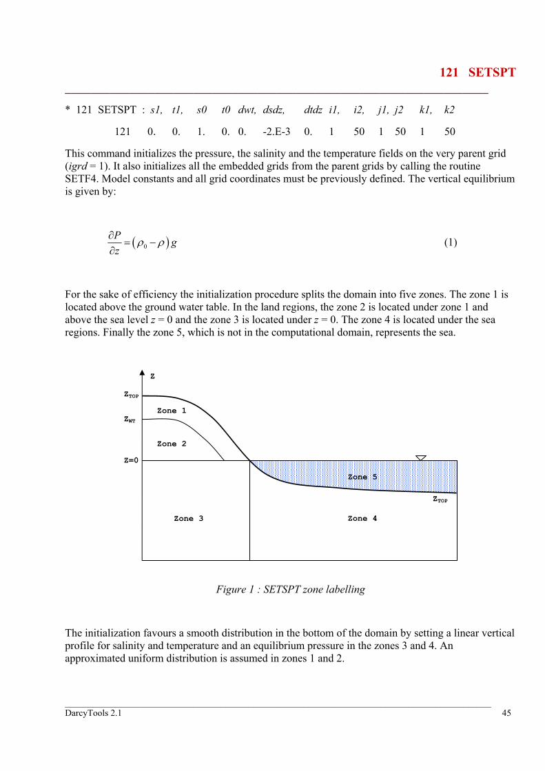
This command initializes the pressure, the salinity and the temperature fields on the very parent grid (igrd = 1). It also initializes all the embedded grids from the parent grids by calling the routine SETF4. Model constants and all grid coordinates must be previously defined. The vertical equilibrium is given by:
( )0P gz
ρ ρ∂= −
∂ (1)
For the sake of efficiency the initialization procedure splits the domain into five zones. The zone 1 is located above the ground water table. In the land regions, the zone 2 is located under zone 1 and above the sea level z = 0 and the zone 3 is located under z = 0. The zone 4 is located under the sea regions. Finally the zone 5, which is not in the computational domain, represents the sea.
Figure 1 : SETSPT zone labelling
The initialization favours a smooth distribution in the bottom of the domain by setting a linear vertical profile for salinity and temperature and an equilibrium pressure in the zones 3 and 4. An approximated uniform distribution is assumed in zones 1 and 2.
Zone 4Zone 3
Zone 2
Zone 1
Z=0
Zone 5
Z
ZWT
ZTOP
ZTOP

_____________________________________________________________________________________________ DarcyTools 2.1 46
Zone 1 & 2:
( )
1
1
0 ( 1, 1) 0( )S T WT WT
S ST T
P g z z g zρ ρ ρ
= = = − − +
(2)
Zone 3:
0
0
( 1, 1) 0 0 ( )S T WT
SS S zzTT T zz
P g z g f zρ ρ
∂ = + ∂∂ = + ∂
= −
(3)
Zone 4:
( )
0
0
0 ( 0, 0) 0 0
( )
( )
( )
Top
Top
S T top Top
SS S z zzTT T z zz
P g z g f z zρ ρ ρ
∂ = + − ∂∂ = + − ∂
= − − −
(4)
Zone 5:
( )
0
0
0 ( 0, 0)S T
S ST T
P g zρ ρ
= = = −
(5)
with the function f0, accordingly to the density state law, such as:
( )2 20 1 0 2 0 1 0 2 0
2
1 2 0 1 2 0
2 23
2 2
( ) ( ) ( )
( 2 ) ( 2 ( ))2
3
f x x S S T T T T
x S TS T Tz z
x S Tz z
ρ ρ
ρ
α α β β
α α β β
α β
= + − − − − +
∂ ∂ + − + − + ∂ ∂ ∂ ∂
− ∂ ∂
(6)
and where the ground water table altitude is given by the depth dWT (>0) and the formula (10) so that setting a very large value for dWT (e.g. 1.E20) fixes the ground water table at sea level z = 0.

_____________________________________________________________________________________________ DarcyTools 2.1 47
( )max 0,WT top WTz z d= − (7)
topz represents the altitude of the top boundary cell face center.
( )( , , 1) ( 1, , 1) ( , 1, 1) ( 1, 1, 1)14Top i j nk i j nk i j nk i j nkz z z z z+ + + + + + + += + + + (8)
Finally, the routine SETSPT can partially initialize the salinity, pressure and temperature fields by specifying the footprint i1, i2, j1, j2, k1, k2 on the very parent grid.
Meaning of parameters:
s1 ...... salinity for z>0 t1 ...... temperature for z>0 s0 …… salinity for z = 0 t0 …… temperature for z = 0 dwt ….. depth of the water table (>0) for z>0 dsdz …. salinity gradient (<0) dtdz …. temperature gradient (<0) i1, i2 … setting's footprint x-definition j1, j2 … setting's footprint y-definition k1, k2 … setting's footprint z-definition
_____________________________________________________________________________________________ DarcyTools 2.1 48
122 SETBOSS __________________________________________________________________
* 122 SETBOSSS : ivar, igrd, itype, i1, i2, j1, j2, k1, k2, it1, it2, qsrc, qphi
122 1 1 0 1 50 1 50 1 20 1 100 9.81E23 1E20
122 2 1 1 1 50 1 1 1 20 1 100 0 0
This command sets the automatic boundary/sink/source conditions which are implemented by DarcyTools. Those conditions concern the variable whose index in the X sub-array is ivar and apply to the specified footprint of the igrd grid. To operate with time dependent computations the footprint notion is extended to the time steps it1, it2. This routine implements two kinds of boundary/sink/source conditions. With the first kind, itype=0, the values qsrc and qphi are uniformly applied to the entire footprint. With the second kind, itype=1, the values qsrc and qphi are not used and Dirichlet boundary conditions are applied to the footprint in order to freeze the variable to its previous time step value. Boundary/sink/source conditions apply in the order of the SETBOSS calls. Hence, when overlapping, only the last definition applies to the footprint intersection.
Meaning of parameters:
ivar ......... index of the variable in the X sub-array igrd ......... index of the grid i1, i2 ........ setting's footprint x-definition j1, j2 ........ setting's footprint y-definition k1,k2 ....... setting's footprint z-definition it1, it2 ...... setting's footprint t-definition qsrc ......... qsrc value to apply in the footprint qphi ......... qphi value to apply in the footprint itype ........ type of condition 0 = uniform values 1 = fixed values in time
_____________________________________________________________________________________________ DarcyTools 2.1 49
123 SETTECF __________________________________________________________________
* 123 SETTECF : fname, title, isbin
123 ‘TecOut’ ‘ ’ 1
This command creates a file named fname for saving a Tecplot data set. The file can be binary or ascii depending on isbin. The Tecplot files ID are associated to the SETTECF calling order, starting from one. If the title string is empty, the title of the run is applied to the file.
Meaning of parameters:
fname ........ name (including path) of the file to create title ........ title of the data set isbin ........ set to 1 for creating a binary file 0 for creating an ascii file
124 SETTECZ __________________________________________________________________
* 124 SETTECZ : ifile, igrd, i1, i2, ifr, j1, j2, jfr, k1, k2, kfr
124 1 1 1 50 2 1 60 2 1 80 1
This command defines a zone that will be added to the Tecplot data set ifile previously created by a SETTECF call. Each zone is attached to a single grid and the data are exported from n1 to n2 with a nfr increment for allowing the extraction of lines, planes or partial domain data.
Meaning of parameters:
ifile ....... index of TECPLOT file igrd ......... index of the grid associated to the zone i1, i2, ifr .... x-footprint and frequency for data extraction j1, j2, jfr .... y-footprint and frequency for data extraction k1, k2, kfr ... z-footprint and frequency for data extraction

_____________________________________________________________________________________________ DarcyTools 2.1 50
125 SETTECB __________________________________________________________________
* 125 SETTECB : ifile, vname, iaction, value
125 1 ‘X1P’ 0 0.
125 1 ‘PERM1’ 3 0.
This routine adds the sub-array named vname to the list of variables to be output in the Tecplot data set ifile. The added sub-array must be common to all the grids of all the zones defined in the data set.
Meaning of parameters:
ifile ........ index of TECPLOT file vname ........ name of the variable to add in the data set iaction ...... modifying action before output (0) no action (1) phi+value (2) phi*value (3) log10(phi) (4) ln(phi) value ........ value for the action when needed
The iaction facility can be used when non-dimensional output is desired or when some other scaling is involved.

_____________________________________________________________________________________________ DarcyTools 2.1 51
126 SETTEC1 __________________________________________________________________
* 126 SETTEC1 : ifile, isgrd
126 1 1
This command specifies the kind of mesh that is to be automatically included into the Tecplot dataset ifile. When isgrid=0 no mesh is added. When isgrid=1 only the mesh linking the cell centres (i.e. the DarcyTools variables location) is added. When isgrd=2 a dummy zone containing the DarcyTools grid is added in first position before returning to the variables location mesh. The default setting is isgrd=2.
Meaning of parameters:
ifile ........ index of TECPLOT file isgrd ........kind of grid to be included 0 = no mesh 1 = only mesh linking the cell centres 2 = add a first zone with a mesh linking vertexes
127 SETTEC2 __________________________________________________________________
* 127 SETTEC2 : ifile, it1, it2, itfr
127 1 11 50 2
This command defines the time domain and increment for creating Tecplot zones. It allows reducing the number of zones and therefore the size of the produced Tecplot file. The defaults values are:
it1 = nstep
it2 = nstep
itfr = 1
A null value for it1 means that a zone will be created for the initialization time.
Meaning of parameters:
ifile ........ index of TECPLOT file it1, it2 ...... istep boundary for TECPLOT's zones creation itfr ......... istep frequency for TECPLOT's zones creation
_____________________________________________________________________________________________ DarcyTools 2.1 52
128 SETTEC3 __________________________________________________________________
* 128 SETTEC3 : ifile, ivar
128 1 2
This command sets up a trigger for creating a new Tecplot zone after each call of the routine SOLVE concerning the variable ivar on the grid associated to the zone. The default value is ivar=0 and means that zones are only created at the end of each time step according to the frequency definition it1, it2, itfr from SETTEC2.
129 SETPRECO __________________________________________________________________
* 129 SETPRECO : precdif
129 0.
This command sets the automatic preconditioning artificial diffusion coefficient for the coupled correction operator. The default value is null and means that no preconditioning is applied. The automatic preconditioning is set by DarcyTools before calling USRPRECO so that users can add a second effect by programming. The automatic preconditioning technique consists in adding the value 7.2 × precdif to the central coefficient and the value precdif to the neighbour coefficients of the second equation of the correction operator.

_____________________________________________________________________________________________ DarcyTools 2.1 53
130 SETSTORE __________________________________________________________________
* 130 SETSTORE : name, igrd
130 ‘M1’ 1
This command marks the sub-array named name associated to the grid igrd for intermediary output into the ROF file. The grid coordinates xv, yv and zv, as well as all the variables are automatically output into the ROF after the last time step and shouldn’t be specified by this routine if not needed before.
131 SETRST __________________________________________________________________
* 131 SETRST : irst
131 1
This command switches ON a restarting computation from a previous ROF file. Since the default setting is “do not restart” this routine has to be called only when a restart is desired and has no dummy arguments. The parameter irst controls wheter the time-value should be reset to 0. or pick up the value from the restart file. irst = 1 reads the value from the restart file, while irst = 0 resets time to 0.0.
_____________________________________________________________________________________________ DarcyTools 2.1 54
132 SETROF1 __________________________________________________________________
* 132 SETROF1 : istep1, istep2, istepfr
132 10 100 10
This command sets the range and frequency of the ROF outputs. It should be called after SETSTEP since the default values are:
istep1 = nstep
istep2 = nstep
istepfr = 1
Meaning of parameters:
istep1 ....... first istep value for ROF intermediary ouput istep2 ....... last istep value for ROF intermediary ouput itfr ......... istep frequency for ROF intermediary ouput
133 SETF4 __________________________________________________________________
* 133 SETF4 : vname, igrd
133 ‘X1S’ 2
This command sets, on the grid igrd, the value of the sub-array named vname from the array having the same name on the parent grid. This implies that igrd is an embedded grid and that vname is valid for both the embedded and the parent grid. No interpolation is performed. The parent values are considered to be uniform inside the parent grid cells.
_____________________________________________________________________________________________ DarcyTools 2.1 55
134 SETFLUX __________________________________________________________________
* 134 SETFLUX : igrd, iflu
134 3 1
This routine sets the kind of parent grid’s boundary conditions that DarcyTools must implement for the specified embedded grid. When iflu=1 the fluxes at parent footprint boundaries are set from the fluxes of the child (embedded) grid igrd. When iflu=0, the parent footprint boundaries values are fixed to the child grid mean local values. The default value is iflu=0.
135 SETHIST1 __________________________________________________________________
* 135 SETHIST1 : i, j, k, igrd, iv, title
135 10 20 30 1 0 ‘Spot Value’
This command defines a new graph for the real time DarcyTools visualization. When i=j=k=0 the graph is for RESIDUALS. When i=0 or j=0 or k=0 and only one of them, the graph is for PROFILES along the (j,k), (i,k) or (i,j) line. When none of i, j or k is null the graph is for SPOT VALUES and i, j, k represents the indexes of the point to plot. The graph is attached to the grid igrd and the writing in HISTxx files is trigged by solving the variable iv unless iv=0. In that case the writing occurs at the end of the time step.
Meaning of parameters:
i, j, k ........ position indexes igrd ......... index of the grid iv ........... index of the variable trigging the file writting title ........ title of the graph (35 characters long)
_____________________________________________________________________________________________ DarcyTools 2.1 56
136 SETHIST2 __________________________________________________________________
* 136 SETHIST2 : igra, vname, label
136 1 ‘X1P’ ‘Pressure’
This routine adds a variable to the graph igra for being drawn. The variable is a sub-array defined both by its name vname and by the grid index associated to the graph. The number of variables per graph is limited to 10. This routine also assigns a label for the variable plot.
Meaning of parameters:
igra ........ graph index in order of the creation via SETHIST1 vname .... name of variable associated to igrid of the graph label ....... a label for the variable (10 characters long)
137 SETSERV __________________________________________________________________
* 137 SETSURV : iport
137
This routine sets the port ID of the darcytools-serv server for communication with the monitoring of HIST files. The default value is 0 and means that the server port has not been change during the installation process (i.e. 1961).
_____________________________________________________________________________________________ DarcyTools 2.1 57
1001 GRGTEC __________________________________________________________________
* 1001 GRGTEC : fname, title, isbin
1001 ‘Tecgrid’ ‘ ‘ 1
This command generates a Tecplot file, which can be used to check the grid before any simulations are attempted. The file can be ascii or binary depending on isbin. Default is no output.
1002 GRGFILE __________________________________________________________________
* 1002 GRGFILE : fname
1002 ‘xyz’
This command sets the file name fname for the grid data. Default is ‘xyz’.

_____________________________________________________________________________________________ DarcyTools 2.1 58
1003 GRGTOP __________________________________________________________________
* 1003 GRGTOP : fname
1003 ‘topography’
This routine sets the file name fname for reading the topography. Independently of the coordinate system of the very parent grid, the topography files are UNFORMATED files, read as follows:
read(iu) ni,nj do j = 1, nj + 1 do i= 1, ni + 1 read (iu) x (i, j), y (i, j), z (i, j) enddo enddo
When the very parent grid is BFC:s or CART the X and Y set are respectively the lines x(i,nj+1) and y(ni+1,j). When the very parent grid is CART the top Z value is z(ni+1,nj+1).
Default is no topography, i.e. ztop = 0. When the file name is ‘user’ or ‘USER’, no file is read but the user subroutine TOPOG, in fif.f, is called.
1004 GRGPCOS __________________________________________________________________
* 1004 GRGPCOS : icosp
1004 3
This command sets the coordinate system of the very parent grid (1 = BFC, 2 = BFC:s and 3 = CARTESIAN). Default is BFC:s.

_____________________________________________________________________________________________ DarcyTools 2.1 59
1005 GRGXDIS __________________________________________________________________
* 1005 GRGXDIS : x0, x1, x2, x3, nx1, nx2, nx3
1005 0 10. 20. 50. 10 20 10
This command sets the x coordinate distribution.
The tree zones are: one expanding/contracting followed by a uniform grid size and finally an expanding/contracting part.
Meaning of parameters:
x0 ........... west abscissa (node 1) x1 ........... west abscissa of zone 2 (node nx1+1) x2 ........... east abscissa of zone 2 (node nx1+nx2+1) x3 ........... east abscissa (node nx1+nx2+nx3+1) nx1 ......... number of cells in zone 1 nx2 ......... number of cells in zone 2 nx3 ......... number of cells in zone 3
Default: x0 = x2 = x3 = 0. x1 = 10, nx1 = 10, nx2 = nx3 = 0.
1006 GRGYDIS __________________________________________________________________
* 1006 GRGYDIS : y0, y1, y2, y3, ny1, ny2, ny3
1006 0 10. 20. 50. 10 20 10
This command sets the y coordinate distribution.
The tree zones are: one expanding/contracting followed by a uniform grid size and finally an expanding/contracting part.
Meaning of parameters:
y0 ........... west abscissa (node 1) y1 ........... west abscissa of zone 2 (node ny1+1) y2 ........... east abscissa of zone 2 (node ny1+ny2+1) y3 ........... east abscissa (node ny1+ny2+ny3+1) ny1 ......... number of cells in zone 1 ny2 ......... number of cells in zone 2 ny3 ......... number of cells in zone 3
Default: y0 = y2 = y3 = 0. y1 = 10, ny1 = 10, ny2 = ny3 = 0.

_____________________________________________________________________________________________ DarcyTools 2.1 60
1007 GRGZDIS __________________________________________________________________
* 1007 GRGZDIS : z3, z4, z5, nz1, nz2, nz3, nz4, nz5 * 1 d1(1) * .. .. * nz1 d1(nz1) 1007 -100. -200. -500. 2 10 0 10 20 + 1 5. + 2 8. The z-distribution is specified according to a five zone partitioning.
zone 1: user given distribution by cell sizes (d1) from top and for n1 cells. d1(i) = z(n-i + 1) - z(n - i) with n = n1 + n2 + n3 + n4 + n5
zone 2. (hyperbolic) tangent distribution of n2 cells that fits a soil/rock surface at z2 and the lower boundary of zone 1.
zone 3: (hyperbolic) tangent distribution with the first node coinciding to the last node of zone 2 and with last node such as z (n4 + n5 + 1) = z3.
zone 4: uniform distribution between the last node of zone 3 and z4. The last node is such as z (n5 + 1) = z4.
zone 5: (hyperbolic) tangent distribution with the first node (n5+1) coinciding to the last node of zone 4 and with last node such as z(1) = z5.
The total number of grid nodes along the z direction is n = n1 + n2 + n3 + n4 + n5 + 1.
n1, n2, n3, n4 or n5 may be null to discard the corresponding zone.
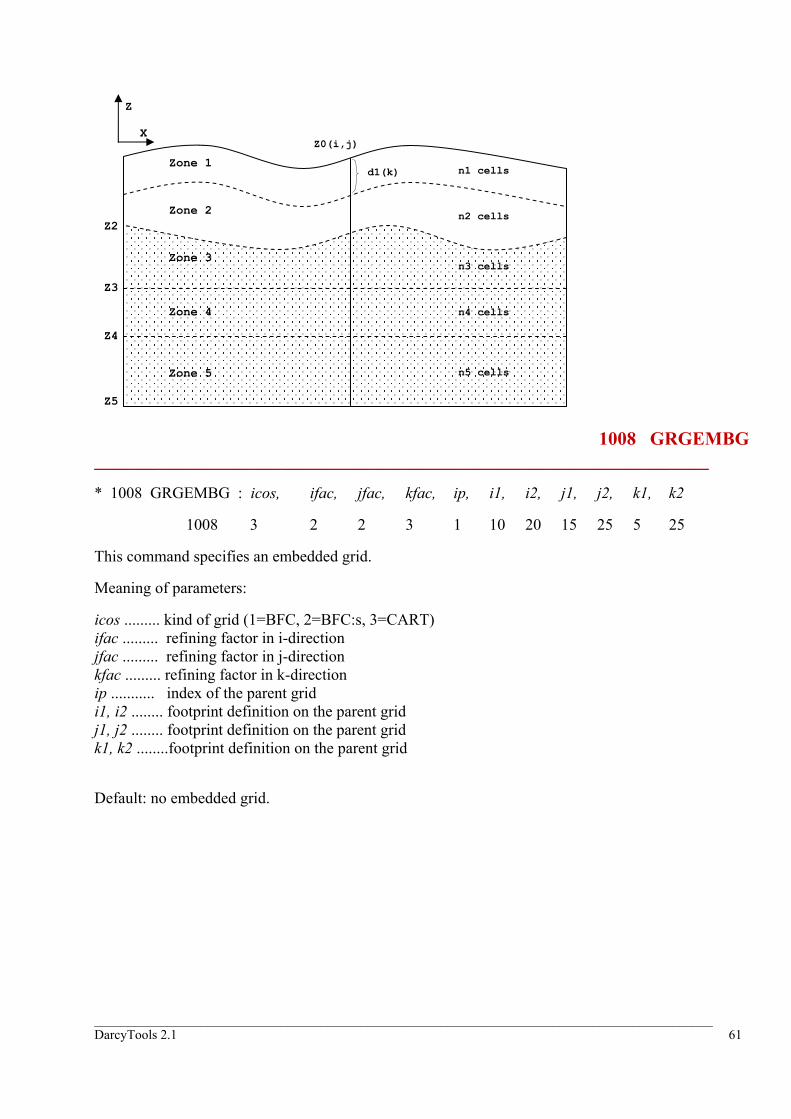
_____________________________________________________________________________________________ DarcyTools 2.1 61
1008 GRGEMBG __________________________________________________________________
* 1008 GRGEMBG : icos, ifac, jfac, kfac, ip, i1, i2, j1, j2, k1, k2
1008 3 2 2 3 1 10 20 15 25 5 25
This command specifies an embedded grid.
Meaning of parameters:
icos ......... kind of grid (1=BFC, 2=BFC:s, 3=CART) ifac ......... refining factor in i-direction jfac ......... refining factor in j-direction kfac ......... refining factor in k-direction ip ........... index of the parent grid i1, i2 ........ footprint definition on the parent grid j1, j2 ........ footprint definition on the parent grid k1, k2 ........footprint definition on the parent grid
Default: no embedded grid.
Zone 5
Zone 4
Zone 2
Zone 1 d1(k) n1 cells
n2 cells
n4 cells
n5 cells
Z0(i,j)
Z5
Z4
X
Z
Z3
Zone 3 n3 cells
Z2

_____________________________________________________________________________________________ DarcyTools 2.1 62
1009 GRGZTOP __________________________________________________________________
* 1009 GRGZTOP : ztop
1009 -450
This command sets the z-coordinate of the upper boundary. Default = 0.0
1010 GRGROC __________________________________________________________________
* 1010 GRGROC : fname
1010 ‘SoilRock’
This command sets the file name for reading the soilrock topography. Regarding the file format, see command 1003 GRGTOP.
_____________________________________________________________________________________________ DarcyTools 2.1 63
1011 GRGDROC __________________________________________________________________
* 1011 GRGDROC : dmin
1011 50.
It is not possible to let the soilrock surface reach ground level as the thicknesses of zones 1 and 2 would then be zero. By setting dmin to a suitable value the soilrock surface is “pressed down”.
dmin: minimum distance between ground level and soilrock surface.
Note: GRIDGEN will print a warning when dmin is activated, in order to alert the user of the modified property specification.
1012 GRGZROC __________________________________________________________________
* 1012 GRGZROC : zrock
1012 -50.
This command sets a uniform value to the soilrock surface level.

_____________________________________________________________________________________________ DarcyTools 2.1 64
2001 FRGGRD __________________________________________________________________
* 2001 FRGGRD : igrid, fname
2001 1 ‘xyz’
This command sets the file name and the grid index for reading the grid coordinates.
2002 FRGSEED __________________________________________________________________
* 2002 FRGSEED : seed
2002 0.917
This command sets the random number generator seed.
_____________________________________________________________________________________________ DarcyTools 2.1 65
2003 FRGWKD __________________________________________________________________
* 2003 FRGWKD : wkdivh1, wkdivh2, wkdivh3
2003 100. 100. 100.
When isolated fractures or clusters are identified and removed the domain is subdivided, as part of the algorithm. The speed of the algorithm is affected by how the subdivision is made; wkdivh* is therefore accessible to specify the subdivision in the three coordinate directions.
It is recommended that wkdivh* is two to ten times the smallest fracture considered. A sensitivity study may give the optimum value.
Default values: 1500. 1500. 1500.
2004 FRGNRD __________________________________________________________________
* 2004 FRGNRD : nxrd, nyrd
2004 100 100
Used for inhomogeneous fractures, see comments for command 2008.
Default values: 1000 1000

_____________________________________________________________________________________________ DarcyTools 2.1 66
2005 FRGNLD __________________________________________________________________
* 2005 FRGNLD : nld
2005 1 000 000
An array dimension related to the total number of fractures generated. If an error print out related to nld is given, this number may need to be larger.
Default value. 1 000 000
2006 FRGOFN __________________________________________________________________
* 2006 FRGOFN : id, fname
2006
This command sets the output files names. The index ordering of the OFNAMES array is as follows: 1- FRCSETx.DAT 2- FREVOLx.DAT 3- FWSx.DAT 4- STORAx.DAT 5- CONDXx.DAT 6- DIFFXx.DAT 7- CONDYx.DAT 8- DIFFYx.DAT 9- CONDZx.DAT 10- DIFFZx.DAT These names should not be modified.

_____________________________________________________________________________________________ DarcyTools 2.1 67
2007 FRGKNWF __________________________________________________________________
* 2007 FRGKNWF : fname
2007 ‘Fracdata’
This command reads the file fname and adds fractures to the list of known fractures.

_____________________________________________________________________________________________ DarcyTools 2.1 68
2008 FRGKNW __________________________________________________________________
* 2008 FRGKNW : inhomf, htknsf, frevolf, fwsrff storaf, conduf, diffuf
* x1, y1, z1, x2, y2, z2, x3, y3, z3
* vkirf1, vkirf2, vkirf3, lewirf1, lewirf2, rcorrf, fsdevf, fwsdevf, ssdevf, csdevf, dsdevf
2008 0 1. 0.005 20. 1.E-6 1.E-4 1.E-10
9.2 -1. 12.1 90. 101 -73 9.2 -1. -6.
This three line command adds a known fracture to the list. If inhomf = 0 (meaning that the fracture is homogeneous) the third line does not need to be specified.
Meaning of parameters:
inhomf……....a homogeneous fracture is specified by 0, an inhomogeneous by 1 htknsf ……... half thickness of fracture frevolf………fracture porosity (in %) fwsrff………..flow wetted surface (m2/m3) storaf……….specific storativity conduf………hydraulic conductivity diffuf………..diffusion coefficient
iii zyx , , …….coordinates for the triangular fracture
An inhomogeneous fracture specification is activated by setting inhomf = 1. A number of additional parameters then need to be considered. The triangle is first divided into a number of equal rectangles by a rectangular grid. The length and width of the rectangles are specified by a parameter lewirf, with first index corresponds to length and second to width. A vector vkirf, with three indexes, specifies the orientation of the grid by the condition that the “length” sides of the rectangles shall be parallel to the orthogonal projection of vkirf onto the fracture plane.
A random number with a multivariate normal distribution is then generated, by the method described in Report 1, Appendix C. The correlation length of the random number field is denoted rcorrf and the correlation lengths in the fracture plane are obtained by multiplying rcorrf with the length and width of the rectangles.
The amplitude is controlled by the specification of the standard deviation, for the variable in question.
Thus:
vkirf* vector for orientation of anisotropy lewirf* length and width of rectangles, covering the fracture plane rcorrf correlation length of random numbers fsdevf standard deviation of porosity fwsdevf standard deviation of flow wetted surface ssdevf standard deviation of storativity csdevf standard deviation of conductivity dsdevf standard deviation diffusivity

_____________________________________________________________________________________________ DarcyTools 2.1 69
When specifying inhomogeneous fractures, command 2004 FRGNRD may need to be considered. nxrd and ngrd give the dimensioning of the arrays used for the rectangles described above. A error print out results if nxrd or nyrd are given to small values.
2009 FRGRANF __________________________________________________________________
* 2009 FRGRANF : fname
2009 ‘RANFRAC’
This command reads the file fname and adds its fractures to the list of random fractures.

_____________________________________________________________________________________________ DarcyTools 2.1 70
2010 FRGRAN1 __________________________________________________________________
* 2010 FRGRAN1 : igenf, lfl, lfh thknsf, frevof, storaf, diffuf, fwsrff
1 10 10.1 0.01 1E-3 1E-6 1E-10 1
This command should always be used together with 2011, as this is the first part of the specification of random fractures.
Meaning of parameters:
igenf……….if 1 the set is generated; 0 ignores the set lfl ……...…..smallest size of the fractures in the set lfh……… ....largest size of the fractures in the set thknsf………thickness of fractures in the set frevof………porosity of the fractures storaf………specific storativity diffuf………diffusion coefficient fwsrff……... flow wetted surface (m2/m3)

_____________________________________________________________________________________________ DarcyTools 2.1 71
2011 FRGRAN2 __________________________________________________________________
* 2011 FRGRAN2 : iset, tcsta, tcstb, tcstc, tcstd, lreff, expidf, idreff, lambdf1, lambdf2, lambdf3
1 1.E-4 0 1.E-4 0.2 500 -2.6 4.E-6 0. 0. 0.
This command should always be used together with 2010, as this is the second part of the specification of random fractures.
Meaning of parameters:
iset……….index to set; refers to the sets given in 2010
...........The relation between transmissivity, , and length, , is given by:
tcstatcstb
T Ltcstctcstd
( ) ( )
( )/100
if
T tcsta L tcstb ran tcstd
T tcstc T tcstc
= × ×× + ×
> =
where ran is a uniform random number in the interval -0.5 to 0.5.
lreff………….a reference length in the power law expidf………..exponent in the power law idreff…….......intensity factor in the power law
...........321
lambdflambdflambdf
gives the position on the sphere for a Fisher-distribution. The length of the vector (given by the three components) gives the kappa in the Fisher-distribution.

_____________________________________________________________________________________________ DarcyTools 2.1 72
3001 TKRIN __________________________________________________________________
* 3001 TKRIN : fname
3001 ‘xyz’
This command specifies the input file, that is to be translated horizontally and rotated around a vertical axes.
3002 TKROUT __________________________________________________________________
* 3002 TKROUT : fname
3002 ‘xyzrot’
This command specifies the output file, i e the file with translated and rotated coordinates.

_____________________________________________________________________________________________ DarcyTools 2.1 73
3003 TKRTRF __________________________________________________________________
* 3003 TKRTRF : dx, dy, degree
3003 100. 10. 40.
The horizontal translation is given by dx and dy, and the rotation by degree (anticlockwise).
4000 SBRTITLE __________________________________________________________________
* 4000 SBRTITLE : title
4000 ‘NEWMODEL’
By default the SUBROF file has the same title as the parent grid. This command gives the opportunity to set a new title to the SUBROF file.

_____________________________________________________________________________________________ DarcyTools 2.1 74
4001 SBRGIN __________________________________________________________________
* 4001 SBRGIN : fname
4001 ‘xyz’
This command specify the input grid file.
4002 SBRGOUT __________________________________________________________________
* 4002 SBRGOUT : fname
4002 ‘xyz.out’
This command specify the output grid file, generated by SUBROF.
_____________________________________________________________________________________________ DarcyTools 2.1 75
4003 SBRRIN __________________________________________________________________
* 4003 SBRRIN : fname
4003 ‘rof’
This command specify the input ROF file.
4004 SBRROUT __________________________________________________________________
* 4004 SBRROUT : fname
4004 ‘rofout’
This command specify the output ROF file.

_____________________________________________________________________________________________ DarcyTools 2.1 76
4005 SBRPDEF __________________________________________________________________
* 4005 SBRPDEF : icos, ifac, jfac, kfac, ip, i1, i2, j1, j2, k1, k2
4005 2 3 2 4 1 10 20 20 30 5 15
This command defines how the new ROF should be generated.
icos ......... kind of grid (1=BFC, 2=BFC:s, 3=CART) ifac ......... refining factor in i-direction jfac ......... refining factor in j-direction kfac ......... refining factor in k-direction ip ........... index of the parent grid i1, i2 ........ footprint definition on the parent grid j1, j2 ........ footprint definition on the parent grid k1, k2 ........footprint definition on the parent grid
4006 SBRTEC __________________________________________________________________
* 4006 SBRTEC : fname, title, isbin
4006 ‘TecSBR’ ‘ ‘ 1
This command generates a Tecplot file, which can be used to check the generated ROF. The file can be ascii or binary depending on isbin (0 = ascii, 1 = binary ).

_____________________________________________________________________________________________ DarcyTools 2.1 77
5 Property Generation (prpgen.f ) The included property generation file is only an example. It is expected that this program will be further developed, as it should be the place where external data (RVS, SICADA, GIS, etc) is introduced and allowed to influence the property fields.

_____________________________________________________________________________________________ DarcyTools 2.1 78
PROGRAM PROPGEN C C-----This program generates property files for SOLVE. C C --It reads the grid coordinates from XYZ C --It reads FRCPRP (Fracture properties) from GEHYCO C --It reads data from external data sources. C --It generates INDGRD, the index grid property file C --It generates the property files for SOLVE C * Set the dimensions * ------------------ parameter (ni=100, nj=100, nk=100) dimension xv(ni+1),yv(nj+1),zv(ni+1,nj+1,nk+1) dimension conduc(ni,nj,nk,3),diffus(ni,nj,nk,3) dimension frevol(ni,nj,nk),fwsurf(ni,nj,nk),storat(ni,nj,nk) dimension pme(ni,nj), poros(ni,nj,nk) C Read Grid coordinates from file "XYZ" C ====================================== WRITE(6,*) 'Read in grid' C Read in fracture properties from file "FRCPRP.dat" C ================================================= C C Note: -frevol is free volume in cell, not porosity open (unit=80, file='condx1.dat', form='UNFORMATTED') open (unit=81, file='condy1.dat', form='UNFORMATTED') open (unit=82, file='condz1.dat', form='UNFORMATTED') open (unit=83, file='frevol1.dat', form='UNFORMATTED') do 160 k=1, nk do 160 j=1, nj do 160 i=1, ni read(83) frevol(i,j,k) read(80) conduc(i,j,k,1) read(81) conduc(i,j,k,2) read(82) conduc(i,j,k,3) 160 continue close (unit=60) WRITE(6,*) 'Read in Fracture properties' C --Read in data from external sources C =================================== WRITE(6,*) 'Read in data from external sources' Figure 5-1. Example of prpgen.f
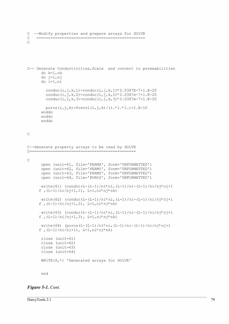
_____________________________________________________________________________________________ DarcyTools 2.1 79
C --Modify properties and prepare arrays for SOLVE C =============================================== C C-- Generate Conductivities,Scale and convert to permeabilities do k=1,nk do j=1,nj do i=1,ni conduc(i,j,k,1)=conduc(i,j,k,1)*2.0387E-7+1.E-20 conduc(i,j,k,2)=conduc(i,j,k,2)*2.0387e-7+1.E-20 conduc(i,j,k,3)=conduc(i,j,k,3)*2.0387e-7+1.E-20 poros(i,j,k)=frevol(i,j,k)/(1.*1.*1.)+1.E-10 enddo enddo enddo C C--Generate property arrays to be read by SOLVE C============================================== C open (unit=61, file='PERMX', form='UNFORMATTED') open (unit=62, file='PERMY', form='UNFORMATTED') open (unit=63, file='PERMZ', form='UNFORMATTED') open (unit=64, file='POROS', form='UNFORMATTED') write(61) (conduc(L-(L-1)/ni*ni,(L-1)/ni-(L-1)/ni/nj*nj+1 f ,(L-1)/ni/nj+1,1), L=1,ni*nj*nk) write(62) (conduc(L-(L-1)/ni*ni,(L-1)/ni-(L-1)/ni/nj*nj+1 f ,(L-1)/ni/nj+1,2), L=1,ni*nj*nk) write(63) (conduc(L-(L-1)/ni*ni,(L-1)/ni-(L-1)/ni/nj*nj+1 f ,(L-1)/ni/nj+1,3), L=1,ni*nj*nk) write(64) (poros(L-(L-1)/ni*ni,(L-1)/ni-(L-1)/ni/nj*nj+1 f ,(L-1)/ni/nj+1), L=1,ni*nj*nk) close (unit=61) close (unit=62) close (unit=63) close (unit=64) WRITE(6,*) 'Generated arrays for SOLVE' end Figure 5-1. Cont.

_____________________________________________________________________________________________ DarcyTools 2.1 80
6 Fortran Input File (fif.f ) 6.1 Why needed? The CIF-commands have been designed to handle most “standard” applications. It is however easy to find situations where it is impossible to handle the problem specification by this method:
- Transient source terms, that may be based on measured data (for example pumping in a borehole).
- Fluid properties that are a function of calculated variables (for example pressure effects on viscosity).
- Boundary conditions that need to be specified as a function of space and time coordinates.
DarcyTools provides a Fortran input file (fif.f ), where more advanced problem specifications can be formulated.
6.2 How to use First of all a word of warning may be in place. The fif.f offers great flexibility, but it also requires more skill and caution of the user. It is up to the user to check that the coding is correct.
The fif.f is visited after the CIF-commands have been interpreted and hence overwrites these. Some parts are also visited every time step or sweep, which needs to be considered when, for example, transient conditions are to be specified.
Probably the best way to learn how to use fif.f is by way of examples; such examples will be given later in this section together with explaining comments. A few general comments may however be useful:
- All variables are stored in a one-dimensional array called the F-array. When using or modifying a variable, one thus has to find its place in the F-array.
- To help the user, a number of “service routines” have been created. These will, for example, help the user to find a variable in the F-array or modify some fluid property.
- When fif.f has been modified, it is of course required that it is recompiled and a new executable is created.
The structure of the F-array and the utility routines are described in the Appendices.
An empty fif.f is given in Figure 6-1. As can be seen it consists of a number of subroutines and the user’s task is to program one or several of these. In the comments the input and output variables are described. In most of the subroutines a declaration “dimension f (*)” is found; this is the above mentioned F-array.
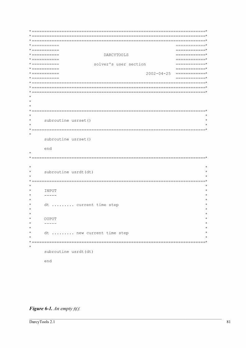
_____________________________________________________________________________________________ DarcyTools 2.1 81
*======================================================================* *======================================================================* *======================================================================* *=========== ============* *=========== ============* *=========== DARCYTOOLS ============* *=========== ============* *=========== solver's user section ============* *=========== ============* *=========== 2002-04-25 ============* *=========== ============* *======================================================================* *======================================================================* *======================================================================* * * * *======================================================================* * * * subroutine usrset() * * * *======================================================================* * subroutine usrset() end * *======================================================================* * * * subroutine usrdt(dt) * * * *======================================================================* * * * INPUT * * ----- * * * * dt ......... current time step * * * * * * OUPUT * * ----- * * * * dt ......... new current time step * * * *======================================================================* * subroutine usrdt(dt) end Figure 6-1. An empty fif.f.
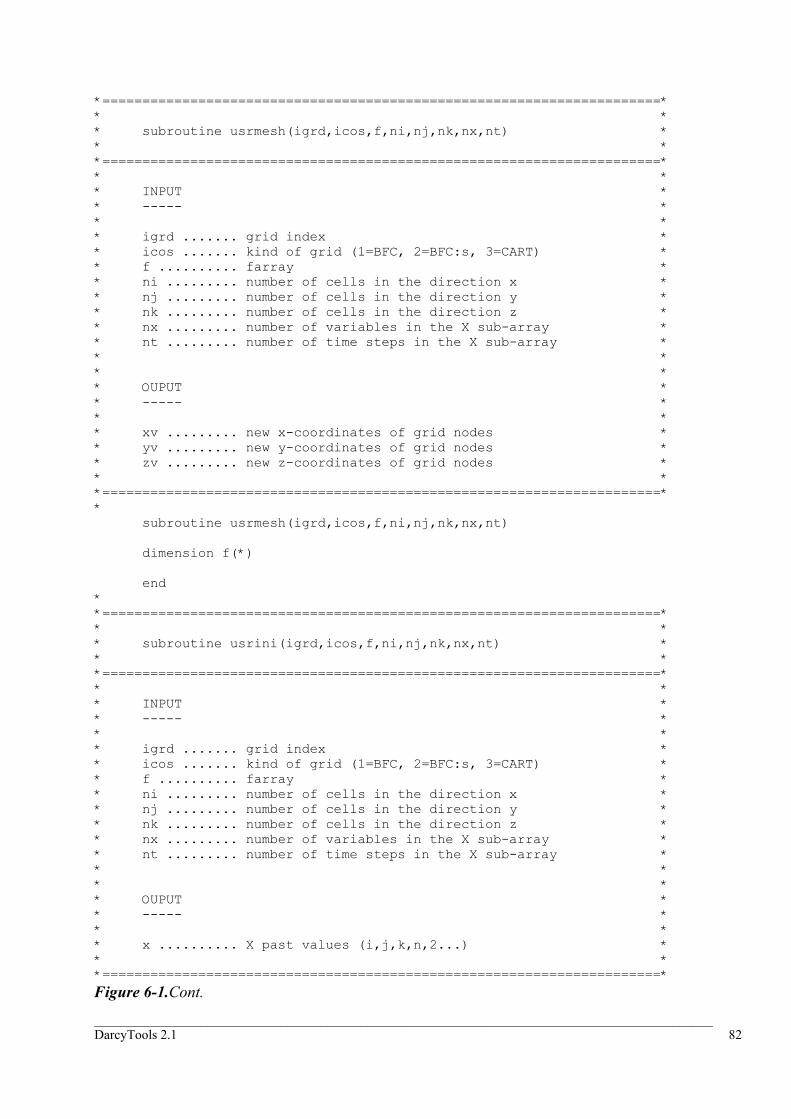
_____________________________________________________________________________________________ DarcyTools 2.1 82
*======================================================================* * * * subroutine usrmesh(igrd,icos,f,ni,nj,nk,nx,nt) * * * *======================================================================* * * * INPUT * * ----- * * * * igrd ....... grid index * * icos ....... kind of grid (1=BFC, 2=BFC:s, 3=CART) * * f .......... farray * * ni ......... number of cells in the direction x * * nj ......... number of cells in the direction y * * nk ......... number of cells in the direction z * * nx ......... number of variables in the X sub-array * * nt ......... number of time steps in the X sub-array * * * * * * OUPUT * * ----- * * * * xv ......... new x-coordinates of grid nodes * * yv ......... new y-coordinates of grid nodes * * zv ......... new z-coordinates of grid nodes * * * *======================================================================* * subroutine usrmesh(igrd,icos,f,ni,nj,nk,nx,nt) dimension f(*) end * *======================================================================* * * * subroutine usrini(igrd,icos,f,ni,nj,nk,nx,nt) * * * *======================================================================* * * * INPUT * * ----- * * * * igrd ....... grid index * * icos ....... kind of grid (1=BFC, 2=BFC:s, 3=CART) * * f .......... farray * * ni ......... number of cells in the direction x * * nj ......... number of cells in the direction y * * nk ......... number of cells in the direction z * * nx ......... number of variables in the X sub-array * * nt ......... number of time steps in the X sub-array * * * * * * OUPUT * * ----- * * * * x .......... X past values (i,j,k,n,2...) * * * *======================================================================* Figure 6-1.Cont.
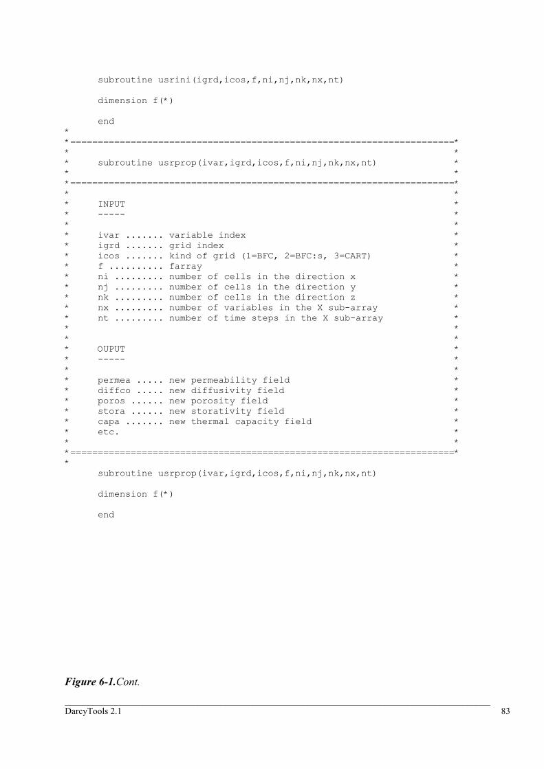
_____________________________________________________________________________________________ DarcyTools 2.1 83
subroutine usrini(igrd,icos,f,ni,nj,nk,nx,nt) dimension f(*) end * *======================================================================* * * * subroutine usrprop(ivar,igrd,icos,f,ni,nj,nk,nx,nt) * * * *======================================================================* * * * INPUT * * ----- * * * * ivar ....... variable index * * igrd ....... grid index * * icos ....... kind of grid (1=BFC, 2=BFC:s, 3=CART) * * f .......... farray * * ni ......... number of cells in the direction x * * nj ......... number of cells in the direction y * * nk ......... number of cells in the direction z * * nx ......... number of variables in the X sub-array * * nt ......... number of time steps in the X sub-array * * * * * * OUPUT * * ----- * * * * permea ..... new permeability field * * diffco ..... new diffusivity field * * poros ...... new porosity field * * stora ...... new storativity field * * capa ....... new thermal capacity field * * etc. * * * *======================================================================* * subroutine usrprop(ivar,igrd,icos,f,ni,nj,nk,nx,nt) dimension f(*) end Figure 6-1.Cont.
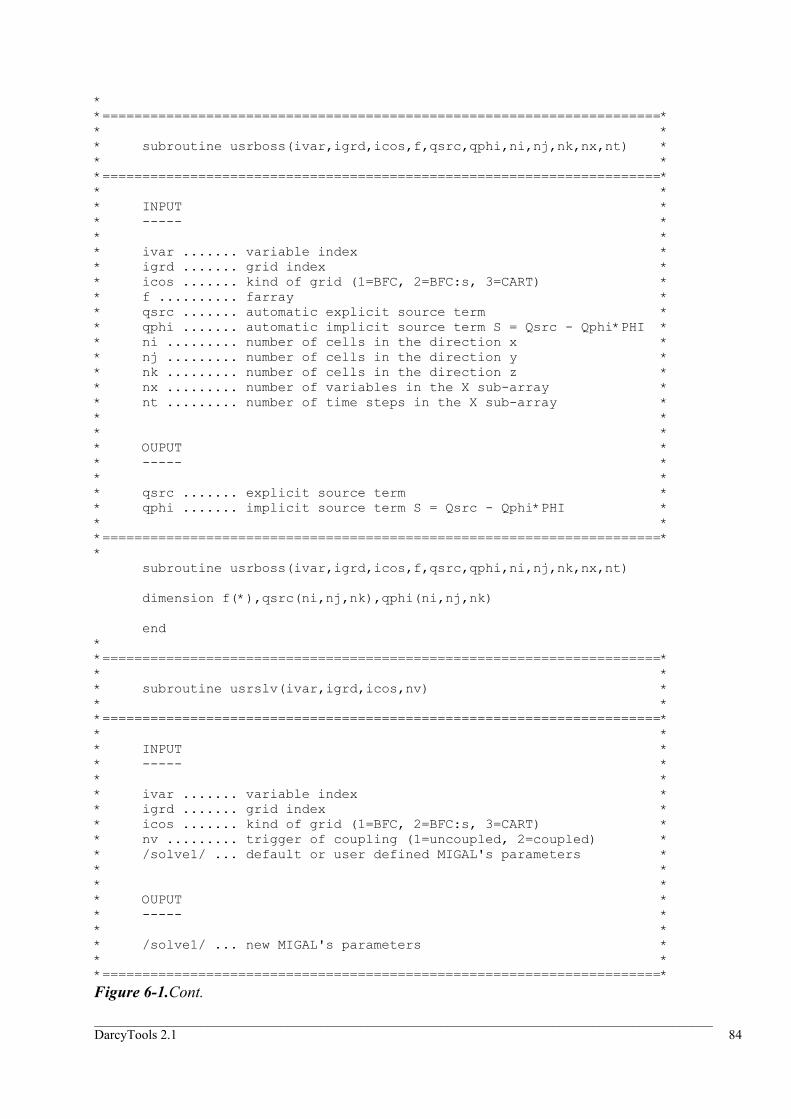
_____________________________________________________________________________________________ DarcyTools 2.1 84
* *======================================================================* * * * subroutine usrboss(ivar,igrd,icos,f,qsrc,qphi,ni,nj,nk,nx,nt) * * * *======================================================================* * * * INPUT * * ----- * * * * ivar ....... variable index * * igrd ....... grid index * * icos ....... kind of grid (1=BFC, 2=BFC:s, 3=CART) * * f .......... farray * * qsrc ....... automatic explicit source term * * qphi ....... automatic implicit source term S = Qsrc - Qphi*PHI * * ni ......... number of cells in the direction x * * nj ......... number of cells in the direction y * * nk ......... number of cells in the direction z * * nx ......... number of variables in the X sub-array * * nt ......... number of time steps in the X sub-array * * * * * * OUPUT * * ----- * * * * qsrc ....... explicit source term * * qphi ....... implicit source term S = Qsrc - Qphi*PHI * * * *======================================================================* * subroutine usrboss(ivar,igrd,icos,f,qsrc,qphi,ni,nj,nk,nx,nt) dimension f(*),qsrc(ni,nj,nk),qphi(ni,nj,nk) end * *======================================================================* * * * subroutine usrslv(ivar,igrd,icos,nv) * * * *======================================================================* * * * INPUT * * ----- * * * * ivar ....... variable index * * igrd ....... grid index * * icos ....... kind of grid (1=BFC, 2=BFC:s, 3=CART) * * nv ......... trigger of coupling (1=uncoupled, 2=coupled) * * /solve1/ ... default or user defined MIGAL's parameters * * * * * * OUPUT * * ----- * * * * /solve1/ ... new MIGAL's parameters * * * *======================================================================* Figure 6-1.Cont.
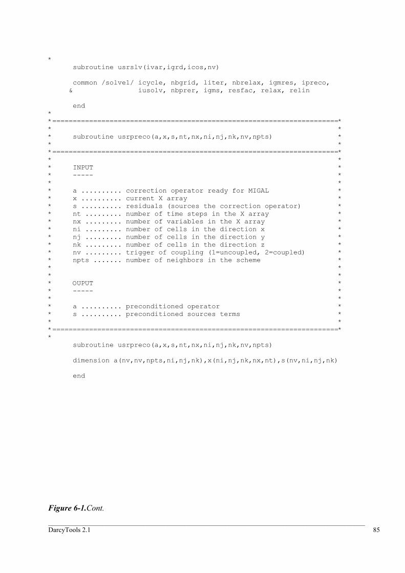
_____________________________________________________________________________________________ DarcyTools 2.1 85
* subroutine usrslv(ivar,igrd,icos,nv) common /solve1/ icycle, nbgrid, liter, nbrelax, igmres, ipreco, & iusolv, nbprer, igms, resfac, relax, relin end * *======================================================================* * * * subroutine usrpreco(a,x,s,nt,nx,ni,nj,nk,nv,npts) * * * *======================================================================* * * * INPUT * * ----- * * * * a .......... correction operator ready for MIGAL * * x .......... current X array * * s .......... residuals (sources the correction operator) * * nt ......... number of time steps in the X array * * nx ......... number of variables in the X array * * ni ......... number of cells in the direction x * * nj ......... number of cells in the direction y * * nk ......... number of cells in the direction z * * nv ......... trigger of coupling (1=uncoupled, 2=coupled) * * npts ....... number of neighbors in the scheme * * * * * * OUPUT * * ----- * * * * a .......... preconditioned operator * * s .......... preconditioned sources terms * * * *======================================================================* * subroutine usrpreco(a,x,s,nt,nx,ni,nj,nk,nv,npts) dimension a(nv,nv,npts,ni,nj,nk),x(ni,nj,nk,nx,nt),s(nv,ni,nj,nk) end Figure 6-1.Cont.
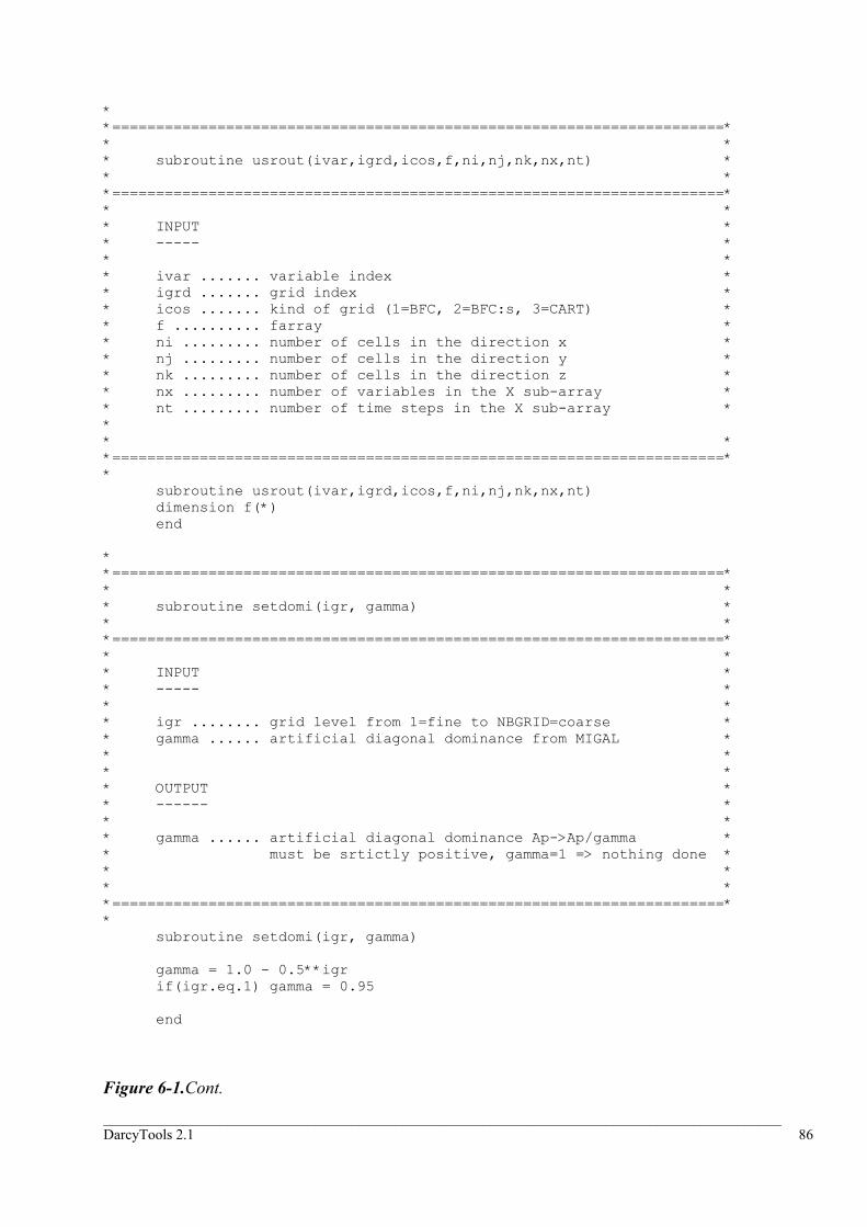
_____________________________________________________________________________________________ DarcyTools 2.1 86
* *======================================================================* * * * subroutine usrout(ivar,igrd,icos,f,ni,nj,nk,nx,nt) * * * *======================================================================* * * * INPUT * * ----- * * * * ivar ....... variable index * * igrd ....... grid index * * icos ....... kind of grid (1=BFC, 2=BFC:s, 3=CART) * * f .......... farray * * ni ......... number of cells in the direction x * * nj ......... number of cells in the direction y * * nk ......... number of cells in the direction z * * nx ......... number of variables in the X sub-array * * nt ......... number of time steps in the X sub-array * * * * *======================================================================* * subroutine usrout(ivar,igrd,icos,f,ni,nj,nk,nx,nt) dimension f(*) end * *======================================================================* * * * subroutine setdomi(igr, gamma) * * * *======================================================================* * * * INPUT * * ----- * * * * igr ........ grid level from 1=fine to NBGRID=coarse * * gamma ...... artificial diagonal dominance from MIGAL * * * * * * OUTPUT * * ------ * * * * gamma ...... artificial diagonal dominance Ap->Ap/gamma * * must be srtictly positive, gamma=1 => nothing done * * * * * *======================================================================* * subroutine setdomi(igr, gamma) gamma = 1.0 - 0.5**igr if(igr.eq.1) gamma = 0.95 end Figure 6-1.Cont.
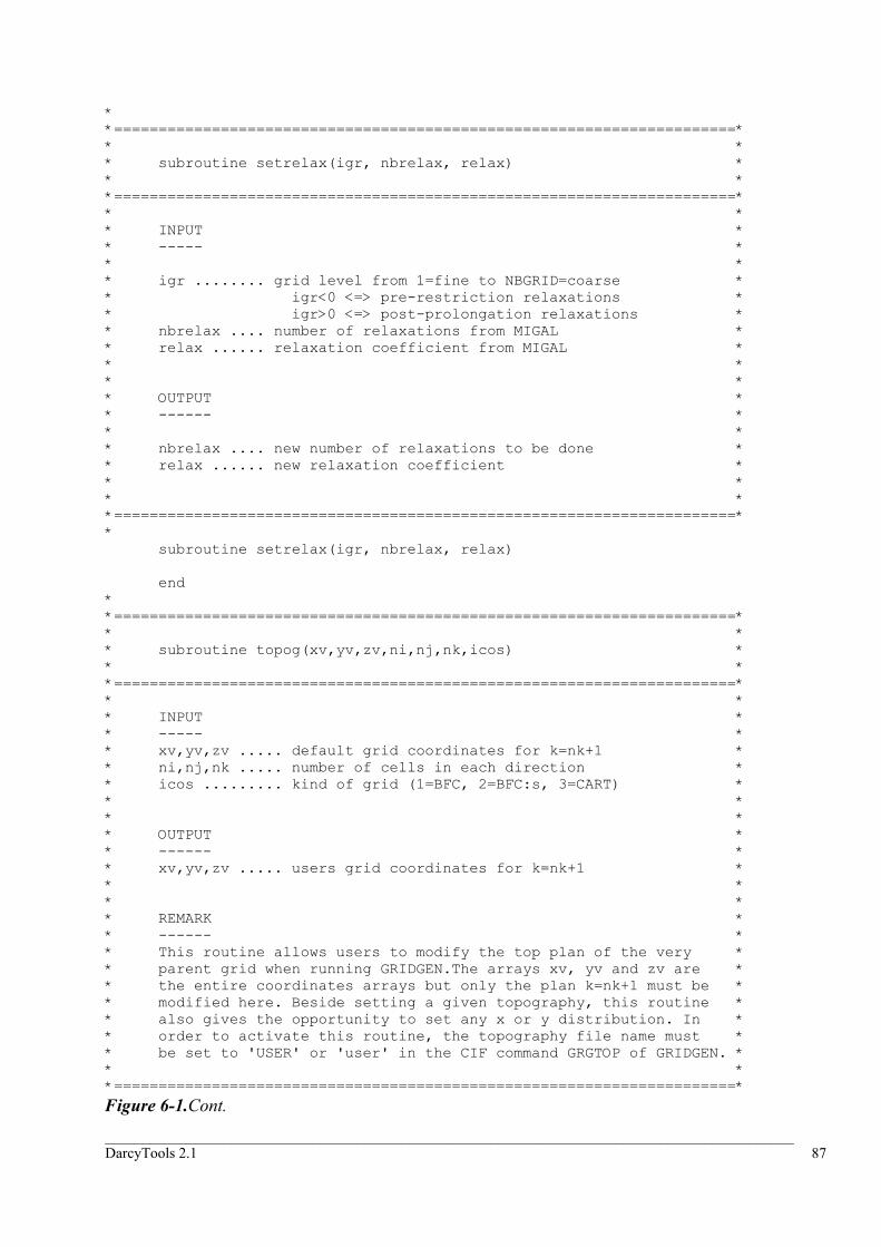
_____________________________________________________________________________________________ DarcyTools 2.1 87
* *======================================================================* * * * subroutine setrelax(igr, nbrelax, relax) * * * *======================================================================* * * * INPUT * * ----- * * * * igr ........ grid level from 1=fine to NBGRID=coarse * * igr<0 <=> pre-restriction relaxations * * igr>0 <=> post-prolongation relaxations * * nbrelax .... number of relaxations from MIGAL * * relax ...... relaxation coefficient from MIGAL * * * * * * OUTPUT * * ------ * * * * nbrelax .... new number of relaxations to be done * * relax ...... new relaxation coefficient * * * * * *======================================================================* * subroutine setrelax(igr, nbrelax, relax) end * *======================================================================* * * * subroutine topog(xv,yv,zv,ni,nj,nk,icos) * * * *======================================================================* * * * INPUT * * ----- * * xv,yv,zv ..... default grid coordinates for k=nk+1 * * ni,nj,nk ..... number of cells in each direction * * icos ......... kind of grid (1=BFC, 2=BFC:s, 3=CART) * * * * * * OUTPUT * * ------ * * xv,yv,zv ..... users grid coordinates for k=nk+1 * * * * * * REMARK * * ------ * * This routine allows users to modify the top plan of the very * * parent grid when running GRIDGEN.The arrays xv, yv and zv are * * the entire coordinates arrays but only the plan k=nk+1 must be * * modified here. Beside setting a given topography, this routine * * also gives the opportunity to set any x or y distribution. In * * order to activate this routine, the topography file name must * * be set to 'USER' or 'user' in the CIF command GRGTOP of GRIDGEN. * * * *======================================================================* Figure 6-1.Cont.

_____________________________________________________________________________________________ DarcyTools 2.1 88
* subroutine topog(xv,yv,zv,ni,nj,nk,icos) end * *======================================================================* * * * subroutine soilroc(zv,ni,nj,icos) * * * *======================================================================* * * * INPUT * * ----- * * zv ........... default soil/rock Z coordinates * * ni,nj ........ number of cells in x and y directions * * icos ......... kind of grid (1=BFC, 2=BFC:s, 3=CART) * * * * * * OUTPUT * * ------ * * zv ........... users soil/rock Z coordinates * * * * * * REMARK * * ------ * * This routine allows users to modify the soil/rock plan on the * * very parent grid when running GRIDGEN.When icos=3 zv is a scalar * * value instead of a (ni+1,nj+1) array. In order to activate this * * routine, the soil:rock file name must be set to 'USER' or 'user' * * in the CIF command GRGROC of GRIDGEN. * * * *======================================================================* * subroutine soilroc(zv,ni,nj,icos) end * *======================================================================*
Figure 6-1.Cont.

_____________________________________________________________________________________________ DarcyTools 2.1 89
6.3 Examples of use The five examples to be discussed are taken from the verification cases (see Report 2) and the user is hence advised to study the relevant cases to bring the coding into context. It may also be useful to have a look on the empty fif.f , Figure 6-1, in parallel in order to get the relevant comments about input and output parameters and the position of the subroutine in fif.f.
Subroutine usrmesh
Different grid options are tested in verification Case A4, from where the coding shown in Figure 6-2 is taken.
Comments:
- The routine lfname is used to get the position of the vertex coordinates in the F-array.
- The index for coordinate system, icos, is used to distinguish the BFC (icos = 1) from the BFC:s case (icos = 2).
- The do-loops and the ijk-index give the relevant F-array positions for the x-coordinates ( )lxv ijk+ , y-coordinates ( )lyv ijk+ and the z-coordinates ( )lzv ijk+ .
- For the BFC:s case (icos = 2), the x and y coordinates are only a function of one index as the coordinate system is Cartesian in the horizontal plane.
Subroutine usrprop
In Case E2, dispersion coefficients that are a function of the local velocity are needed. This is clearly a situation that calls for fif.f coding, as we do not know the velocity field before hand. This subroutine, see Figure 6-3, is hence visited at every iteration sweep and the properties are updated.
Comments:
- As in the previous example we need the first location of variables in the F-array. M1 and M3 are mass-fluxes across x and z cell walls (the case is 2D) and X1S and X1T are the variable names for salinity and temperature respectively.
- We are only interested in dispersion coefficients for salinity, hence the statement “if (ivar.eq.2) then “
- Utility routines are used (fn_rho, get_poros, get_diff and set_diff). Details about these can be found in the Appendices.
- Some under-relaxation is used to change the dispersion coefficients smoothly during the iterations.
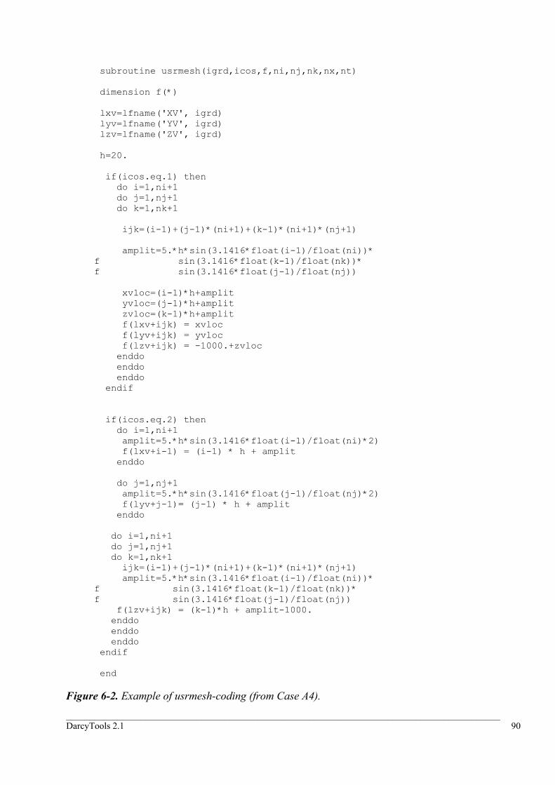
_____________________________________________________________________________________________ DarcyTools 2.1 90
subroutine usrmesh(igrd,icos,f,ni,nj,nk,nx,nt) dimension f(*) lxv=lfname('XV', igrd) lyv=lfname('YV', igrd) lzv=lfname('ZV', igrd) h=20. if(icos.eq.1) then do i=1,ni+1 do j=1,nj+1 do k=1,nk+1 ijk=(i-1)+(j-1)*(ni+1)+(k-1)*(ni+1)*(nj+1) amplit=5.*h*sin(3.1416*float(i-1)/float(ni))* f sin(3.1416*float(k-1)/float(nk))* f sin(3.1416*float(j-1)/float(nj)) xvloc=(i-1)*h+amplit yvloc=(j-1)*h+amplit zvloc=(k-1)*h+amplit f(lxv+ijk) = xvloc f(lyv+ijk) = yvloc f(lzv+ijk) = -1000.+zvloc enddo enddo enddo endif if(icos.eq.2) then do i=1,ni+1 amplit=5.*h*sin(3.1416*float(i-1)/float(ni)*2) f(lxv+i-1) = (i-1) * h + amplit enddo do j=1,nj+1 amplit=5.*h*sin(3.1416*float(j-1)/float(nj)*2) f(lyv+j-1)= (j-1) * h + amplit enddo do i=1,ni+1 do j=1,nj+1 do k=1,nk+1 ijk=(i-1)+(j-1)*(ni+1)+(k-1)*(ni+1)*(nj+1) amplit=5.*h*sin(3.1416*float(i-1)/float(ni))* f sin(3.1416*float(k-1)/float(nk))* f sin(3.1416*float(j-1)/float(nj)) f(lzv+ijk) = (k-1)*h + amplit-1000. enddo enddo enddo endif end Figure 6-2. Example of usrmesh-coding (from Case A4).
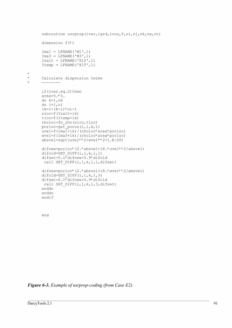
_____________________________________________________________________________________________ DarcyTools 2.1 91
subroutine usrprop(ivar,igrd,icos,f,ni,nj,nk,nx,nt) dimension f(*) Ima1 = LFNAME('M1',1) Ima3 = LFNAME('M3',1) Isalt = LFNAME('X1S',1) Itemp = LFNAME('X1T',1) * * Calculate dispersion terms * -------- if(ivar.eq.2)then area=5.*5. do k=1,nk do i=1,ni ik=i+(k-1)*ni-1 sloc=f(Isalt+ik) tloc=f(Itemp+ik) rholoc=fn_rho(sloc,tloc) porloc=get_poros(i,1,k,1) uvel=f(ima1+ik)/(rholoc*area*porloc) wvel=f(Ima3+ik)/(rholoc*area*porloc) absvel=sqrt(uvel**2+wvel**2+1.E-20) difnew=porloc*(2.*absvel+18.*uvel**2/absvel) difold=GET_DIFF(i,1,k,1,1) difset=0.1*difnew+0.9*difold call SET_DIFF(i,1,k,1,1,difset) difnew=porloc*(2.*absvel+18.*wvel**2/absvel) difold=GET_DIFF(i,1,k,1,3) difset=0.1*difnew+0.9*difold call SET_DIFF(i,1,k,1,3,difset) enddo enddo endif end
Figure 6-3. Example of usrprop-coding (from Case E2).
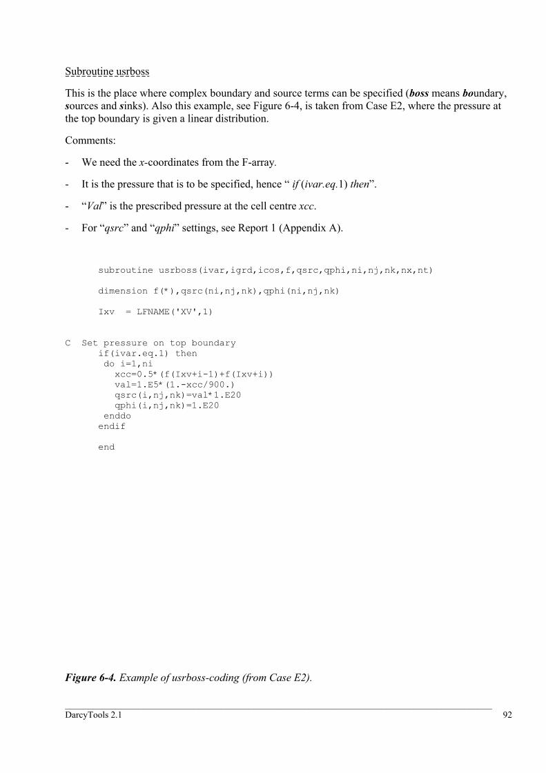
_____________________________________________________________________________________________ DarcyTools 2.1 92
Subroutine usrboss
This is the place where complex boundary and source terms can be specified (boss means boundary, sources and sinks). Also this example, see Figure 6-4, is taken from Case E2, where the pressure at the top boundary is given a linear distribution.
Comments:
- We need the x-coordinates from the F-array.
- It is the pressure that is to be specified, hence “ if (ivar.eq.1) then”.
- “Val” is the prescribed pressure at the cell centre xcc.
- For “qsrc” and “qphi” settings, see Report 1 (Appendix A).
subroutine usrboss(ivar,igrd,icos,f,qsrc,qphi,ni,nj,nk,nx,nt) dimension f(*),qsrc(ni,nj,nk),qphi(ni,nj,nk) Ixv = LFNAME('XV',1) C Set pressure on top boundary if(ivar.eq.1) then do i=1,ni xcc=0.5*(f(Ixv+i-1)+f(Ixv+i)) val=1.E5*(1.-xcc/900.) qsrc(i,nj,nk)=val*1.E20 qphi(i,nj,nk)=1.E20 enddo endif end
Figure 6-4. Example of usrboss-coding (from Case E2).

_____________________________________________________________________________________________ DarcyTools 2.1 93
Subroutine usrout
As the name indicates this is the place where additional output is generated. In the example (Case E6), see Figure 6-5, output for comparison with an analytical solution is generated.
Comments:
- We need access to the mass fluxes (M1) and the z-coordinates (zv) in the F-array.
- Only one set of profiles is needed, hence the statement “ if (ivar.eq.1. and. istep.eq.nstep)”.
- The utility routine “iufree” is used to get a free logical unit number.
- Two commons are used to get access to “isweep” and “nstep”.
- ijk gives the location of a scalar located at a cell centre, while ijkv gives the location of vertex coordinates (there is one more vertex value than scalar value in a coordinate direction).
subroutine usrout(ivar,igrd,icos,f,ni,nj,nk,nx,nt) dimension f(*) common /const2/ nstep,nsweep,nvar1,nvar2,nitc1, & nvar3,nvar4, nitc2,nvar5,nvar6,nitg common /const3/ istep,isweep,dum1,itc,dum2,itg,t lvu=lfname('M1', igrd) lzv=lfname('ZV', igrd) if(ivar.eq.1.and.istep.eq.nstep) then ifile=iufree() OPEN(unit=ifile,file='TWOFL.dat') j=1 i=ni/2 area=0.25*0.25 do k=1,nk ijk=i-1+(j-1)*ni+(k-1)*ni*nj ijkv=i-1+(j-1)*(ni+1)+(k-1)*(ni+1)*(nj+1) zcord=0.5*(f(lzv+k-1)+f(lzv+k)) uvel=-f(lvu+ijk)/1000./area c--analytical solution perm=1.e-12 drho=50. emu1=2.E-3 emu2=6.E-3 zsize=10. fact1=sin(3.14159*(zcord+5.)/zsize) fact2=alog((1.+fact1)/(1.-fact1)) qzero=perm*drho*9.81/(emu1+emu2) uanl=qzero*fact2/3.14159 write(ifile,*) zcord, uvel, uanl enddo endif end Figure 6-5. Example of usrout-coding (from Case E6).

_____________________________________________________________________________________________ DarcyTools 2.1 94
Subroutine topog
The coding, see Figure 6-6, is used in Case E5, where the top boundary is given the shape of a sinusoidal function.
Comments:
- As zv is given as a 3D array in the dimension statement, one can access the array by these indexes.
subroutine topog(xv,yv,zv,ni,nj,nk,icos) dimension zv(ni+1,nj+1,nk+1) C---GENERATE TOPOGRAPHY DO j=1,nj+1 DO i=1,ni+1 PId2=3.1416/2. amplit=(10.*sin(2.*3.1416*float(i-1)/ f float(ni)-PId2)+10.)-10.0 zv(i,j,nk+1) = amplit ENDDO ENDDO end
Figure 6-6. Example of topog-coding (from Case E5).

_____________________________________________________________________________________________ DarcyTools 2.1 95
7 A SITE-LABORATORY-EXPERIMENTAL SCALE DEMO
7.1 Introduction In Report 1 results from this Demo Case were presented and discussed. It was also noted that the Demo is generic, but share many features of a real world application.
Here the emphasis is on the set-up of the case in DarcyTools; the CIF and fif.f files, and other programs, will be presented and discussed.
In order to make the presentation self-contained some parts of the presentation of the case will first be repeated.
7.2 The situation studied The situation studied is outlined in Figure 7-1. It is a coastal site, with seawater of a brackish nature (salinity of 1%). We assume a certain precipitation on land and we hence have a density stratification to take into account. Two hills give a certain topography on land. A tunnel, with a certain inflow, will be placed below the small island in the laboratory volume shown in the figure. The focus of the analysis will be on the effects of the tunnel. The situation has a clear resemblance with the Äspö region. The fracture system will however be much simpler in this demo, as compared to the detailed information available for Äspö HRL. Four major fracture zones, shown in Figure 7-1, are assumed to represent the deterministic system. Random fractures will be generated to build a working fracture network.
A summary of the problem specification is given in Table 7-1. It is not the intention to give a complete account of the input data; this is considered to be outside the scope (the specification of the fracture network would be lengthy, for example). A few comments may be needed as a complement to the key features in the table (see also Figure 7-1):
• Domains. The site model covers the whole domain, while the laboratory model is located below the island. The first of these two grids are of the BFC:s type (follows the topography), while the second grid is a cartesian one. The experimental model is placed in the laboratory model, but outside the tunnel area.
• Properties. Porosity is specified for each fracture and fracture zone. The diffusion coefficient is given a value of ten times the value for molecular diffusion for salt; this process is hence insignificant. Transmissivities, orientations, etc for the random fractures are set according to the values found appropriate for Äspö HRL.
• Random fractures. When the fracture network for the site domain is generated, random fracture in the interval 20 → 1000 metres are generated. Those random fractures that intersect the laboratory volume are imported as deterministic fractures to this domain. Random fractures in the interval 10 - 20 metres are then added. The same procedure is repeated for the experimental volume; now with all fractures larger than 10 metres as deterministic and random fractures in the interval 2 – 10 metres.
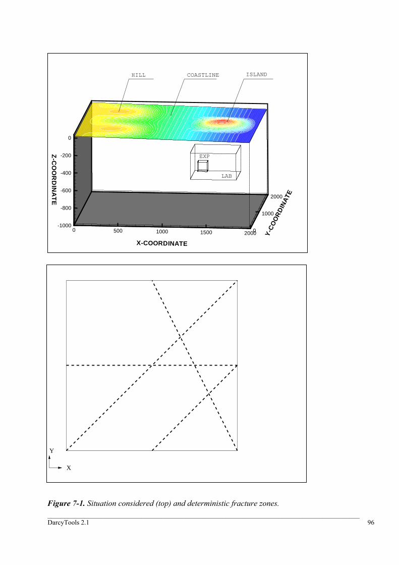
_____________________________________________________________________________________________ DarcyTools 2.1 96
-1000
-800
-600
-400
-200
0
Z-C
OO
RD
INA
TE
0 500 1000 1500 2000
X-COORDINATE
0
1000
2000
Y-C
OO
RD
INA
TE
HILL COASTLINE ISLAND
LAB
EXP
Y
X
Figure 7-1. Situation considered (top) and deterministic fracture zones.

_____________________________________________________________________________________________ DarcyTools 2.1 97
Table 7-1. Summary of problem specification.
Domains and grids Site: 2 x 2 x 1 km3 NX = 100, NY = 100, NZ = 50, ∆ =20
Laboratory: 500 x 500 x 300 m3 NX = 50, NY = 50, NZ = 30, ∆ = 10 Experimental: 100 x 100 x 100 m3 NX = 50, NY =50, NZ = 50 ∆ =2
Properties - Deterministic zones according to Figure 7-1,
Transmissivity = 10-5 m2/s - Random fractures Site: 20 1000 ml = → Laboratory: 10 20 ml = → Experimental: 2 10 ml = →
- Diffusion coefficients: 810− m2/s, constant
- Porosity: 310− , constant
Boundary conditions Top: Precipitation on land , 50 mm/year Pressure and salinity fixed below sea
Vertical boundaries: Zero flux when boundary on land, prescribed pressure and salinity when below sea. Fixed salinity at bottom boundary.
Tunnel : Three tunnel sections are defined; two with a prescribed skin (= 0.01) and one with a prescribed inflow (= 1 l/s).
Groundwater table: As part of the simulation the groundwater table is calculated. The specific yield feature is not activated as we are only considering the steady state.
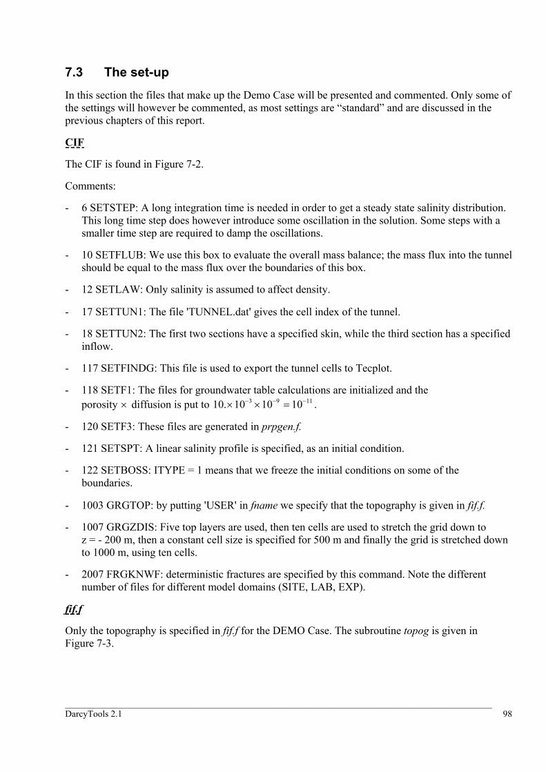
_____________________________________________________________________________________________ DarcyTools 2.1 98
7.3 The set-up In this section the files that make up the Demo Case will be presented and commented. Only some of the settings will however be commented, as most settings are “standard” and are discussed in the previous chapters of this report.
CIF
The CIF is found in Figure 7-2.
Comments:
- 6 SETSTEP: A long integration time is needed in order to get a steady state salinity distribution. This long time step does however introduce some oscillation in the solution. Some steps with a smaller time step are required to damp the oscillations.
- 10 SETFLUB: We use this box to evaluate the overall mass balance; the mass flux into the tunnel should be equal to the mass flux over the boundaries of this box.
- 12 SETLAW: Only salinity is assumed to affect density.
- 17 SETTUN1: The file 'TUNNEL.dat' gives the cell index of the tunnel.
- 18 SETTUN2: The first two sections have a specified skin, while the third section has a specified inflow.
- 117 SETFINDG: This file is used to export the tunnel cells to Tecplot.
- 118 SETF1: The files for groundwater table calculations are initialized and the porosity × diffusion is put to 3 9 1110. 10 10 10− − −× × = .
- 120 SETF3: These files are generated in prpgen.f.
- 121 SETSPT: A linear salinity profile is specified, as an initial condition.
- 122 SETBOSS: ITYPE = 1 means that we freeze the initial conditions on some of the boundaries.
- 1003 GRGTOP: by putting 'USER' in fname we specify that the topography is given in fif.f.
- 1007 GRGZDIS: Five top layers are used, then ten cells are used to stretch the grid down to z = - 200 m, then a constant cell size is specified for 500 m and finally the grid is stretched down to 1000 m, using ten cells.
- 2007 FRGKNWF: deterministic fractures are specified by this command. Note the different number of files for different model domains (SITE, LAB, EXP).
fif.f
Only the topography is specified in fif.f for the DEMO Case. The subroutine topog is given in Figure 7-3.

_____________________________________________________________________________________________ DarcyTools 2.1 99
fractools.f
This is a small program written for the Demo Case, see Figure 7-4. The main task for this program is to read input files, specifying fractures and zones, and write these on a format that can be read by DarcyTools. For the Demo Case, random fractures from a larger domain are specified as deterministic fractures for the next smaller domain; the main part of fractools.f is devoted to this task.
prpgen.f
A property generation program, prpgen.f, is written for each domain. In Figure 7-5, the prpgen.f, for the SITE domain is given. The comments in the program explain the different tasks of this program.

_____________________________________________________________________________________________ DarcyTools 2.1 100
********************************************************** * * * DemoCase * * * * 10 May 2003 * * * ********************************************************** * 1 SETTITLE : title 1 'DEMO CASE' * 2 SETGRDF : fname 2 'xyz' * 3 SETLICM : licence, path 3 'y]GCJ?HJAMTVlxHZmDa' '' * 6 SETSTEP : dt nstep iorder * Run 500 steps with dt=1.e7 and underrealaxtion 0.3, then make * a restart with dt=1.E5 and underrelaxation=0.1. This to damp * oscillations. * 6 1.E7 500 1 6 1.E5 200 1 * 10 SETFLUB : id, i1, i2, j1, j2, k1, k2, igrd 10 1 50 90 30 70 5 40 1 * 12 SETLAW1 : rho0, Trho, alpha1, alpha2, beta1, beta2 12 1000. 0. 0.008 0. 0. 0. * 13 SETLAW2 : visc0, a1, a2, Tvisc, n 13 2.E-3 0. 0. 0. 1 * 16 SETGWT : grlx, facmin 16 0.8 0.001 * 17 SETTUN1 : fname 17 'TUNNEL2.dat' * 18 SETTUN2 : isec, iaction, sink, skin, skmin, skmax, rlx 18 1 1 0. .01 1.E-10 1.E9 .1 18 2 1 0. .01 1.E-10 1.E9 .1 18 3 2 1. .05 1.E-10 1.E9 .1 * 20 SETSLV1 : ivar, igrd, relin, resfac, liter 20 1 0 .1 0.00 6 20 2 0 .1 0.00 6 * 110 SETSWEEP : nsweep, ivar1, ivar2 110 1 1 2 * 115 SETBNDY : ssea, tsea, tland 115 1.0 0.0 0.0 * 117 SETFINDG : igrd, form, fname 117 2 'unformatted' 'INDGRD_2' Figure 7-2. Demo Case, CIF.
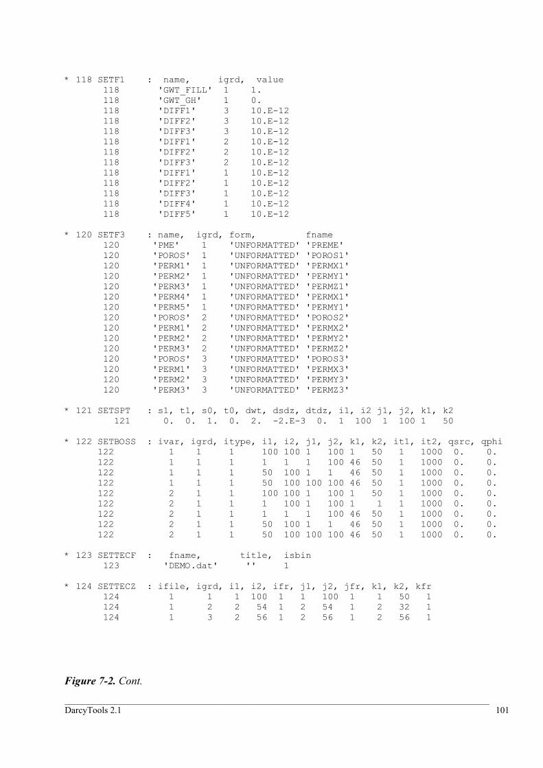
_____________________________________________________________________________________________ DarcyTools 2.1 101
* 118 SETF1 : name, igrd, value 118 'GWT_FILL' 1 1. 118 'GWT_GH' 1 0. 118 'DIFF1' 3 10.E-12 118 'DIFF2' 3 10.E-12 118 'DIFF3' 3 10.E-12 118 'DIFF1' 2 10.E-12 118 'DIFF2' 2 10.E-12 118 'DIFF3' 2 10.E-12 118 'DIFF1' 1 10.E-12 118 'DIFF2' 1 10.E-12 118 'DIFF3' 1 10.E-12 118 'DIFF4' 1 10.E-12 118 'DIFF5' 1 10.E-12 * 120 SETF3 : name, igrd, form, fname 120 'PME' 1 'UNFORMATTED' 'PREME' 120 'POROS' 1 'UNFORMATTED' 'POROS1' 120 'PERM1' 1 'UNFORMATTED' 'PERMX1' 120 'PERM2' 1 'UNFORMATTED' 'PERMY1' 120 'PERM3' 1 'UNFORMATTED' 'PERMZ1' 120 'PERM4' 1 'UNFORMATTED' 'PERMX1' 120 'PERM5' 1 'UNFORMATTED' 'PERMY1' 120 'POROS' 2 'UNFORMATTED' 'POROS2' 120 'PERM1' 2 'UNFORMATTED' 'PERMX2' 120 'PERM2' 2 'UNFORMATTED' 'PERMY2' 120 'PERM3' 2 'UNFORMATTED' 'PERMZ2' 120 'POROS' 3 'UNFORMATTED' 'POROS3' 120 'PERM1' 3 'UNFORMATTED' 'PERMX3' 120 'PERM2' 3 'UNFORMATTED' 'PERMY3' 120 'PERM3' 3 'UNFORMATTED' 'PERMZ3' * 121 SETSPT : s1, t1, s0, t0, dwt, dsdz, dtdz, i1, i2 j1, j2, k1, k2 121 0. 0. 1. 0. 2. -2.E-3 0. 1 100 1 100 1 50 * 122 SETBOSS : ivar, igrd, itype, i1, i2, j1, j2, k1, k2, it1, it2, qsrc, qphi 122 1 1 1 100 100 1 100 1 50 1 1000 0. 0. 122 1 1 1 1 1 1 100 46 50 1 1000 0. 0. 122 1 1 1 50 100 1 1 46 50 1 1000 0. 0. 122 1 1 1 50 100 100 100 46 50 1 1000 0. 0. 122 2 1 1 100 100 1 100 1 50 1 1000 0. 0. 122 2 1 1 1 100 1 100 1 1 1 1000 0. 0. 122 2 1 1 1 1 1 100 46 50 1 1000 0. 0. 122 2 1 1 50 100 1 1 46 50 1 1000 0. 0. 122 2 1 1 50 100 100 100 46 50 1 1000 0. 0. * 123 SETTECF : fname, title, isbin 123 'DEMO.dat' '' 1 * 124 SETTECZ : ifile, igrd, i1, i2, ifr, j1, j2, jfr, k1, k2, kfr 124 1 1 1 100 1 1 100 1 1 50 1 124 1 2 2 54 1 2 54 1 2 32 1 124 1 3 2 56 1 2 56 1 2 56 1 Figure 7-2. Cont.

_____________________________________________________________________________________________ DarcyTools 2.1 102
* 125 SETTECB : ifile, vname action value 125 1 'GWT_FILL' 0 0 125 1 'X1P' 0 0 125 1 'X1S' 0 0 125 1 'INDGRD15' 0 0 125 1 'DARCY-U' 0 0 125 1 'DARCY-V' 0 0 125 1 'DARCY-W' 0 0 125 1 'POROS' 0 0 125 1 'PERM1' 0 0 125 1 'PERM2' 0 0 125 1 'PERM3' 0 0 * 130 SETSTORE : name, igrd 130 GWT_GH 1 130 GWT_FILL 1 * 131 SETRST : 131 * 135 SETHIST : i j k igrd iv title 135 0 0 0 1 2 'Residuals' 135 81 46 31 1 2 'Spot Values (81,46,31)' 135 5 25 0 1 2 'Profile, j=25 i=5' 135 0 0 0 1 2 'Mass balance Grid 1' 135 30 50 48 1 2 'Spot Values (30,50,48)' * 136 SETHIST2 : igra vname label 136 1 'RESP' 'Pressure' 136 1 'RESS' 'Salinity' 136 2 'X1P' 'Pressure' 136 2 'X1S' 'Salinity' 136 3 'GWT_FILL' 'Saturation' 136 3 'X1P' 'Pressure' 136 3 'X1S' 'Salinity' 136 4 'FLUB1' 'Flub1' 136 5 'X1P' 'Pressure' ********************************************************** * * * GRIDGEN setting * * 1001 GRGTEC : fname, title, isbin 1001 'TecXYZ' '' 1 * 1003 GRGTOP : fname 1003 'USER' * 1004 GRGPCOS : icosp 1004 2 * 1005 GRGXDIS : x0, x1, x2, x3, nx1, nx2, nx3 1005 0. 0. 2000. 2000. 0 100 0 * 1006 GRGYDIS : y0, y1, y2, y3, ny1, ny2, ny3 1006 0. 0. 2000. 2000. 0 100 0 Figure 7-2. Cont.

_____________________________________________________________________________________________ DarcyTools 2.1 103
* 1007 GRGZDIS : z3, z4, z5, nz1, nz2, nz3, nz4, nz5 1007 -200. -700. -1000. 5 10 0 25 10 + 1, 2. + 2, 3. + 3, 4. + 4, 5. + 5, 6. * 1008 GRGEMBG : icos, ifac, jfac, kfac, ip, i1, i2, j1, j2, k1, k2 1008 3 2 2 2 1 63 88 38 63 16 30 1008 3 5 5 5 2 10 20 10 20 10 20 ********************************************************** * * * FRACGEN setting * * 2001 FRGGRD : igrd, fname 2001 1 'xyz' * 2002 FRGSEED : seed 2002 0.234 * 2007 FRGKNWF : fname 2007 'FRACSITE' * 2007 'FRACLAB' * 2007 'FRACEXP' * 2010 FRGRAN1 : igenf, lfl, lfh, thknsf, frevof, storaf, diffuf, fwsrff 2010 1 500. 1000. 5. 1.E-3 1.E-6 1.E-10 100. 2010 1 200. 500. 2. 1.E-3 1.E-6 1.E-10 100. 2010 1 100. 200. 1. 1.E-3 1.E-6 1.E-10 100. 2010 1 50. 100. 0.5 1.E-3 1.E-6 1.E-10 100. 2010 1 20. 50. 0.25 1.E-3 1.E-6 1.E-10 100. 2010 0 10. 20. 0.10 1.E-3 1.E-6 1.E-10 100. 2010 0 2. 10. 0.05 1.E-3 1.E-6 1.E-10 100. 2010 1 500. 1000. 5. 1.E-3 1.E-6 1.E-10 100. 2010 1 200. 500. 2. 1.E-3 1.E-6 1.E-10 100. 2010 1 100. 200. 1. 1.E-3 1.E-6 1.E-10 100. 2010 1 50. 100. 0.5 1.E-3 1.E-6 1.E-10 100. 2010 1 20. 50. 0.25 1.E-3 1.E-6 1.E-10 100. 2010 0 10. 20. 0.10 1.E-3 1.E-6 1.E-10 100. 2010 0 2. 10. 0.05 1.E-3 1.E-6 1.E-10 100. Figure 7-2. Cont.

_____________________________________________________________________________________________ DarcyTools 2.1 104
* 2011 FRGRAN2 : iset, tcsta, tcstb, tcstc, lreff, expidf, idreff, lambdf1, lambdf2,lambdf3 2011 1 1.E-5 2.0 1.E-5 500. -2.6 7.E-9 8.487 8.487 0. 2011 2 1.E-5 2.0 1.E-5 500. -2.6 7.E-9 8.487 8.487 0. 2011 3 1.E-5 2.0 1.E-5 500. -2.6 7.E-9 8.487 8.487 0. 2011 4 1.E-5 2.0 1.E-5 500. -2.6 7.E-9 8.487 8.487 0. 2011 5 1.E-5 2.0 1.E-5 500. -2.6 7.E-9 8.487 8.487 0. 2011 6 1.E-5 2.0 1.E-5 500. -2.6 7.E-9 8.487 8.487 0. 2011 7 1.E-5 2.0 1.E-5 500. -2.6 7.E-9 8.487 8.487 0. 2011 8 1.E-5 2.0 1.E-5 500. -2.6 3.E-9 -4.95 4.95 0. 2011 9 1.E-5 2.0 1.E-5 500. -2.6 3.E-9 -4.95 4.95 0. 2011 10 1.E-5 2.0 1.E-5 500. -2.6 3.E-9 -4.95 4.95 0. 2011 11 1.E-5 2.0 1.E-5 500. -2.6 3.E-9 -4.95 4.95 0. 2011 12 1.E-5 2.0 1.E-5 500. -2.6 3.E-9 -4.95 4.95 0. 2011 13 1.E-5 2.0 1.E-5 500. -2.6 3.E-9 -4.95 4.95 0. 2011 14 1.E-5 2.0 1.E-5 500. -2.6 3.E-9 -4.95 4.95 0.
Figure 7-2. Cont.
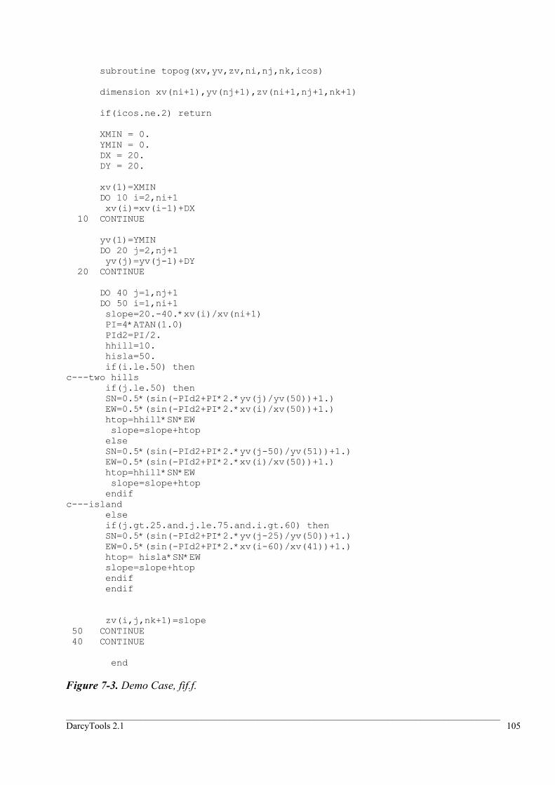
_____________________________________________________________________________________________ DarcyTools 2.1 105
subroutine topog(xv,yv,zv,ni,nj,nk,icos) dimension xv(ni+1),yv(nj+1),zv(ni+1,nj+1,nk+1) if(icos.ne.2) return XMIN = 0. YMIN = 0. DX = 20. DY = 20. xv(1)=XMIN DO 10 i=2,ni+1 xv(i)=xv(i-1)+DX 10 CONTINUE yv(1)=YMIN DO 20 j=2,nj+1 yv(j)=yv(j-1)+DY 20 CONTINUE DO 40 j=1,nj+1 DO 50 i=1,ni+1 slope=20.-40.*xv(i)/xv(ni+1) PI=4*ATAN(1.0) PId2=PI/2. hhill=10. hisla=50. if(i.le.50) then c---two hills if(j.le.50) then SN=0.5*(sin(-PId2+PI*2.*yv(j)/yv(50))+1.) EW=0.5*(sin(-PId2+PI*2.*xv(i)/xv(50))+1.) htop=hhill*SN*EW slope=slope+htop else SN=0.5*(sin(-PId2+PI*2.*yv(j-50)/yv(51))+1.) EW=0.5*(sin(-PId2+PI*2.*xv(i)/xv(50))+1.) htop=hhill*SN*EW slope=slope+htop endif c---island else if(j.gt.25.and.j.le.75.and.i.gt.60) then SN=0.5*(sin(-PId2+PI*2.*yv(j-25)/yv(50))+1.) EW=0.5*(sin(-PId2+PI*2.*xv(i-60)/xv(41))+1.) htop= hisla*SN*EW slope=slope+htop endif endif zv(i,j,nk+1)=slope 50 CONTINUE 40 CONTINUE end Figure 7-3. Demo Case, fif.f.

_____________________________________________________________________________________________ DarcyTools 2.1 106
C PROGRAM FRACTOOLS C C-----This program reads and prepares fracture data for DEMO CASE C 2003-05-10: The program is in a draft form. C C--- Declarations C================= Parameter(nfd=20000,nfDET=4,nfLAB=46040,nfEXP=4456) dimension x(4,nfd),y(4,nfd),z(4,nfd) dimension pkvp(3,8,nfLAB),frevol(nfLAB),fwsurf(nfLAB) dimension storat(nfLAB),conduc(nfLAB) dimension diffus(nfLAB),thickn(nfLAB) OPEN(UNIT=70,FILE='frcset1.dat',form='unformatted') OPEN(UNIT=80,FILE='FRACLAB',form='unformatted') OPEN(UNIT=90,FILE='frcset2.dat',form='unformatted') OPEN(UNIT=91,FILE='FRACEXP',form='unformatted') OPEN(UNIT=71,FILE='zon.dat') OPEN(UNIT=72,FILE='FRACSITE',form='unformatted') C---READ FRACTURE DATA C====================== c--deterministic do 11 ifr=1,nfDET read(71,*) f x(1,ifr),y(1,ifr),z(1,ifr),x(2,ifr),y(2,ifr), f z(2,ifr),x(3,ifr),y(3,ifr),z(3,ifr) 11 continue close(unit=71) c--PRINT DATA TO FILE (FOR INPUT TO DARCYTOOLS) C============================================= do 10 ifr=1,nfDET c---properties inhomf=0 htknsf=10. frevlf=1.E-3 fwsrff=1. storaf=1.E-6 conduf=1.E-5/(2.*htknsf) diffuf=1.e-10 c--coordinates X1=x(1,ifr) X2=x(2,ifr) X3=x(3,ifr) Figure 7-4. Demo Case, fractools.f.
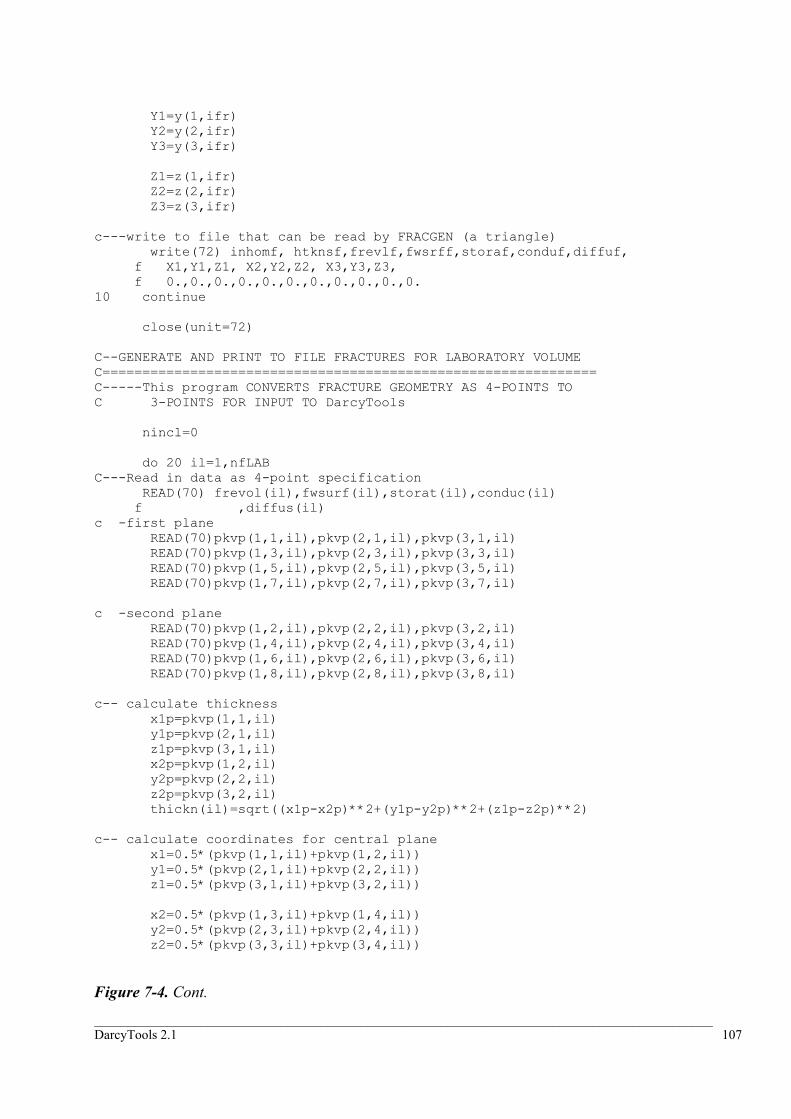
_____________________________________________________________________________________________ DarcyTools 2.1 107
Y1=y(1,ifr) Y2=y(2,ifr) Y3=y(3,ifr) Z1=z(1,ifr) Z2=z(2,ifr) Z3=z(3,ifr) c---write to file that can be read by FRACGEN (a triangle) write(72) inhomf, htknsf,frevlf,fwsrff,storaf,conduf,diffuf, f X1,Y1,Z1, X2,Y2,Z2, X3,Y3,Z3, f 0.,0.,0.,0.,0.,0.,0.,0.,0.,0.,0. 10 continue close(unit=72) C--GENERATE AND PRINT TO FILE FRACTURES FOR LABORATORY VOLUME C============================================================== C-----This program CONVERTS FRACTURE GEOMETRY AS 4-POINTS TO C 3-POINTS FOR INPUT TO DarcyTools nincl=0 do 20 il=1,nfLAB C---Read in data as 4-point specification READ(70) frevol(il),fwsurf(il),storat(il),conduc(il) f ,diffus(il) c -first plane READ(70)pkvp(1,1,il),pkvp(2,1,il),pkvp(3,1,il) READ(70)pkvp(1,3,il),pkvp(2,3,il),pkvp(3,3,il) READ(70)pkvp(1,5,il),pkvp(2,5,il),pkvp(3,5,il) READ(70)pkvp(1,7,il),pkvp(2,7,il),pkvp(3,7,il) c -second plane READ(70)pkvp(1,2,il),pkvp(2,2,il),pkvp(3,2,il) READ(70)pkvp(1,4,il),pkvp(2,4,il),pkvp(3,4,il) READ(70)pkvp(1,6,il),pkvp(2,6,il),pkvp(3,6,il) READ(70)pkvp(1,8,il),pkvp(2,8,il),pkvp(3,8,il) c-- calculate thickness x1p=pkvp(1,1,il) y1p=pkvp(2,1,il) z1p=pkvp(3,1,il) x2p=pkvp(1,2,il) y2p=pkvp(2,2,il) z2p=pkvp(3,2,il) thickn(il)=sqrt((x1p-x2p)**2+(y1p-y2p)**2+(z1p-z2p)**2) c-- calculate coordinates for central plane x1=0.5*(pkvp(1,1,il)+pkvp(1,2,il)) y1=0.5*(pkvp(2,1,il)+pkvp(2,2,il)) z1=0.5*(pkvp(3,1,il)+pkvp(3,2,il)) x2=0.5*(pkvp(1,3,il)+pkvp(1,4,il)) y2=0.5*(pkvp(2,3,il)+pkvp(2,4,il)) z2=0.5*(pkvp(3,3,il)+pkvp(3,4,il)) Figure 7-4. Cont.
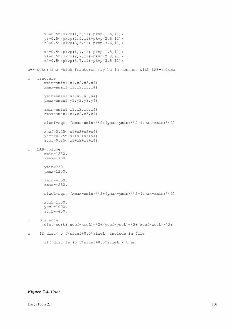
_____________________________________________________________________________________________ DarcyTools 2.1 108
x3=0.5*(pkvp(1,5,il)+pkvp(1,6,il)) y3=0.5*(pkvp(2,5,il)+pkvp(2,6,il)) z3=0.5*(pkvp(3,5,il)+pkvp(3,6,il)) x4=0.5*(pkvp(1,7,il)+pkvp(1,8,il)) y4=0.5*(pkvp(2,7,il)+pkvp(2,8,il)) z4=0.5*(pkvp(3,7,il)+pkvp(3,8,il)) c-- determine which fractures may be in contact with LAB-volume c fracture xmin=amin1(x1,x2,x3,x4) xmax=amax1(x1,x2,x3,x4) ymin=amin1(y1,y2,y3,y4) ymax=amax1(y1,y2,y3,y4) zmin=amin1(z1,z2,z3,z4) zmax=amax1(z1,z2,z3,z4) sizef=sqrt((xmax-xmin)**2+(ymax-ymin)**2+(zmax-zmin)**2) xccf=0.25*(x1+x2+x3+x4) yccf=0.25*(y1+y2+y3+y4) zccf=0.25*(z1+z2+z3+z4) c LAB-volume xmin=1250. xmax=1750. ymin=750. ymax=1250. zmin=-650. zmax=-250. sizeL=sqrt((xmax-xmin)**2+(ymax-ymin)**2+(zmax-zmin)**2) xccL=1500. yccL=1000. zccL=-450. c Distance dist=sqrt((xccf-xccL)**2+(yccf-yccL)**2+(zccf-zccL)**2) c If dist< 0.5*sizef+0.5*sizeL include in file if( dist.le.(0.5*sizef+0.5*sizeL)) then Figure 7-4. Cont.

_____________________________________________________________________________________________ DarcyTools 2.1 109
nincl=nincl+2 C---Print out as two 3-point fractures c---properties inhomf=0 htknsf=thickn(il)/2. frevlf=frevol(il) fwsrff=fwsurf(il) storaf=storat(il) conduf=conduc(il) diffuf=diffus(il) c---write to file that can be read by FRACGEN (two triangles) write(80) inhomf, htknsf,frevlf,fwsrff,storaf,conduf,diffuf, f X1,Y1,Z1, X2,Y2,Z2, X3,Y3,Z3, f 0.,0.,0.,0.,0.,0.,0.,0.,0.,0.,0. write(80) inhomf, htknsf,frevlf,fwsrff,storaf,conduf,diffuf, f X2,Y2,Z2, X3,Y3,Z3, X4,Y4,Z4, f 0.,0.,0.,0.,0.,0.,0.,0.,0.,0.,0. endif 20 continue close(unit=80) close(unit=70) write(6,*) nincl,'triangular fractures in file FRACLAB' C--GENERATE AND PRINT TO FILE FRACTURES FOR EXPERIMENTAL VOLUME C============================================================== C-----This program CONVERTS FRACTURE GEOMETRY AS 4-POINTS TO C 3-POINTS FOR INPUT TO DarcyTools nincl=0 do 30 il=1,nfEXP c C---Read in data as 4-point specification READ(90) frevol(il),fwsurf(il),storat(il),conduc(il) f ,diffus(il) c -first plane READ(90)pkvp(1,1,il),pkvp(2,1,il),pkvp(3,1,il) READ(90)pkvp(1,3,il),pkvp(2,3,il),pkvp(3,3,il) READ(90)pkvp(1,5,il),pkvp(2,5,il),pkvp(3,5,il) READ(90)pkvp(1,7,il),pkvp(2,7,il),pkvp(3,7,il) c -second plane READ(90)pkvp(1,2,il),pkvp(2,2,il),pkvp(3,2,il) READ(90)pkvp(1,4,il),pkvp(2,4,il),pkvp(3,4,il) READ(90)pkvp(1,6,il),pkvp(2,6,il),pkvp(3,6,il) READ(90)pkvp(1,8,il),pkvp(2,8,il),pkvp(3,8,il) Figure 7-4. Cont.

_____________________________________________________________________________________________ DarcyTools 2.1 110
c-- calculate thickness x1p=pkvp(1,1,il) y1p=pkvp(2,1,il) z1p=pkvp(3,1,il) x2p=pkvp(1,2,il) y2p=pkvp(2,2,il) z2p=pkvp(3,2,il) thickn(il)=sqrt((x1p-x2p)**2+(y1p-y2p)**2+(z1p-z2p)**2) c-- calculate coordinates for central plane x1=0.5*(pkvp(1,1,il)+pkvp(1,2,il)) y1=0.5*(pkvp(2,1,il)+pkvp(2,2,il)) z1=0.5*(pkvp(3,1,il)+pkvp(3,2,il)) x2=0.5*(pkvp(1,3,il)+pkvp(1,4,il)) y2=0.5*(pkvp(2,3,il)+pkvp(2,4,il)) z2=0.5*(pkvp(3,3,il)+pkvp(3,4,il)) x3=0.5*(pkvp(1,5,il)+pkvp(1,6,il)) y3=0.5*(pkvp(2,5,il)+pkvp(2,6,il)) z3=0.5*(pkvp(3,5,il)+pkvp(3,6,il)) x4=0.5*(pkvp(1,7,il)+pkvp(1,8,il)) y4=0.5*(pkvp(2,7,il)+pkvp(2,8,il)) z4=0.5*(pkvp(3,7,il)+pkvp(3,8,il)) c-- determine which fractures may be in contact with EXP-volume c fracture xmin=amin1(x1,x2,x3,x4) xmax=amax1(x1,x2,x3,x4) ymin=amin1(y1,y2,y3,y4) ymax=amax1(y1,y2,y3,y4) zmin=amin1(z1,z2,z3,z4) zmax=amax1(z1,z2,z3,z4) sizef=sqrt((xmax-xmin)**2+(ymax-ymin)**2+(zmax-zmin)**2) xccf=0.25*(x1+x2+x3+x4) yccf=0.25*(y1+y2+y3+y4) zccf=0.25*(z1+z2+z3+z4) c Exp-volume xmin=1350. xmax=1450. ymin=850. ymax= 950. zmin=-500. zmax=-400. sizeL=sqrt((xmax-xmin)**2+(ymax-ymin)**2+(zmax-zmin)**2) Figure 7-4. Cont.

_____________________________________________________________________________________________ DarcyTools 2.1 111
xccL=1400. yccL=900. zccL=-450. c Distance dist=sqrt((xccf-xccL)**2+(yccf-yccL)**2+(zccf-zccL)**2) c If dist< 0.5*sizef+0.5*sizeL include in file if( dist.le.(0.5*sizef+0.5*sizeL)) then nincl=nincl+2 C---Print out as two 3-point fractures c---properties inhomf=0 htknsf=thickn(il)/2. frevlf=frevol(il) fwsrff=fwsurf(il) storaf=storat(il) conduf=conduc(il) diffuf=diffus(il) c---write to file that can be read by FRACGEN (two triangles) write(91) inhomf, htknsf,frevlf,fwsrff,storaf,conduf,diffuf, f X1,Y1,Z1, X2,Y2,Z2, X3,Y3,Z3, f 0.,0.,0.,0.,0.,0.,0.,0.,0.,0.,0. write(91) inhomf, htknsf,frevlf,fwsrff,storaf,conduf,diffuf, f X2,Y2,Z2, X3,Y3,Z3, X4,Y4,Z4, f 0.,0.,0.,0.,0.,0.,0.,0.,0.,0.,0. endif 30 continue close(unit=90) close(unit=91) write(6,*) nincl,'triangular fractures in file FRACEXP' end
Figure 7-4. Cont.

_____________________________________________________________________________________________ DarcyTools 2.1 112
PROGRAM PROPGEN C C-----This program generates property files for DEMO Case,SITE C C --It reads the grid coordinates from xyz C --It reads fracture properties as generated by FRACGEN C --It reads data from external data sources. C --It generates INDGRD, the index grid property file C --It generates the property files for SOLVE C * Set dimensions * =============== parameter (nid=100, njd=100, nkd=50) dimension xv(nid+1), yv(njd+1), zv(nid+1,njd+1,nkd+1) dimension conduc(nid,njd,nkd,3), diffus(nid,njd,nkd,3) dimension fwsurf(nid,njd,nkd), frevol(nid,njd,nkd) dimension storat(nid,njd,nkd),pme(nid,njd) dimension perm(nid,njd,nkd,3), poros(nid,njd,nkd) C Read Grid coordinates from file "xyz" C ====================================== open(unit=98,file='xyz',form='unformatted') ires= mesh_p(98,1,nii,njj,nkk,icos,ip,i1,i2,j1,j2,k1,k2) if(ires.ne.0) WRITE(6,*) 'GRID ERROR' ni=nii nj=njj nk=nkk ires = mesh_r(98,1,xv,yv,zv) if(ires.ne.0) WRITE(6,*) 'GRID ERROR' close(unit=98) WRITE(6,*) 'Read in grid' C Read in fracture properties from files C ====================================== C C Note: -frevol is free volume in cell, not porosity open (unit=80, file='condx1.dat', form='UNFORMATTED') open (unit=81, file='condy1.dat', form='UNFORMATTED') open (unit=82, file='condz1.dat', form='UNFORMATTED') open (unit=83, file='frevol1.dat', form='UNFORMATTED') do 160 k=1, nk do 160 j=1, nj do 160 i=1, ni read(80) conduc(i,j,k,1) read(81) conduc(i,j,k,2) read(82) conduc(i,j,k,3) read(83) frevol(i,j,k) 160 continue close (unit=80) close (unit=81) close (unit=82) close (unit=83) WRITE(6,*) 'Read in Fracture properties' Figure 7-5. Demo Case, prpgen.f.

_____________________________________________________________________________________________ DarcyTools 2.1 113
C --Read in data from external sources C =================================== WRITE(6,*) 'Read in data from external sources' C --Modify properties and prepare arrays for SOLVE C =============================================== C-- Generate Porosity and Permeabilities. Add min values. do k=1,nk do j=1,nj do i=1,ni vol=(xv(i+1)-xv(i))*(yv(j+1)-yv(j))*(zv(i,j,k+1)-zv(i,j,k)) do idir=1,3 con=conduc(i,j,k,idir) if(k.eq.50.and.con.lt.2.e-4) conduc(i,j,k,idir)=2.e-4 if(k.eq.49.and.con.lt.2.e-5) conduc(i,j,k,idir)=2.e-5 if(k.eq.48.and.con.lt.2.e-6) conduc(i,j,k,idir)=2.e-6 if(k.eq.47.and.con.lt.2.e-7) conduc(i,j,k,idir)=2.e-7 enddo perm(i,j,k,1)=conduc(i,j,k,1)*2.0387E-7+2.E-16 perm(i,j,k,2)=conduc(i,j,k,2)*2.0387e-7+2.E-16 perm(i,j,k,3)=conduc(i,j,k,3)*2.0387e-7+2.E-16 poros(i,j,k)=frevol(i,j,k)/vol+1.E-6 enddo enddo enddo C--Fill pme array and Scale do j=1,nj do i=1,ni zsurf=0.25*(zv(i,j,nk+1)+zv(i+1,j,nk+1)+ f zv(i,j+1,nk+1)+zv(i+1,j+1,nk+1)) rain=50. pme(i,j)=rain*1.E-3/(3600.*24.*365.)*1. if(zsurf.lt.0.) pme(i,j)=0. enddo enddo WRITE(6,*) 'Arrays for SOLVE ready' C-- Generate property arrays to be read by SOLVE C ============================================ open (unit=61, file='PERMX1', form='UNFORMATTED') open (unit=62, file='PERMY1', form='UNFORMATTED') open (unit=63, file='PERMZ1', form='UNFORMATTED') open (unit=64, file='POROS1', form='UNFORMATTED') open (unit=65, file='PREME', form='UNFORMATTED') write(61) (perm(L-(L-1)/ni*ni,(L-1)/ni-(L-1)/ni/nj*nj+1 f ,(L-1)/ni/nj+1,1), L=1,ni*nj*nk) Figure 7-5. Cont.

_____________________________________________________________________________________________ DarcyTools 2.1 114
write(62) (perm(L-(L-1)/ni*ni,(L-1)/ni-(L-1)/ni/nj*nj+1 f ,(L-1)/ni/nj+1,2), L=1,ni*nj*nk) write(63) (perm(L-(L-1)/ni*ni,(L-1)/ni-(L-1)/ni/nj*nj+1 f ,(L-1)/ni/nj+1,3), L=1,ni*nj*nk) write(64) (poros(L-(L-1)/ni*ni,(L-1)/ni-(L-1)/ni/nj*nj+1 f ,(L-1)/ni/nj+1), L=1,ni*nj*nk) write(65) (pme(L-(L-1)/ni*ni,(L-1)/ni-(L-1)/ni/nj*nj+1) f , L=1,ni*nj*1) close (unit=61) close (unit=62) close (unit=63) close (unit=64) close (unit=65) WRITE(6,*) 'Generated arrays for SOLVE' end
Figure 7-5. Cont.

_____________________________________________________________________________________________ DarcyTools 2.1 115
8 References
Ferry M., 2002. MIGAL. See www.mfrdc.com
Jackson C. P., Andrew R. H. and Todman S., 2000. Self-consistency of heterogeneous continuum porous medium representation of a fractured medium. Water Resources Res., 36(1), 189-202.
Sahimi M., 1995. Flow and transport in porous media and fractured rock. VCH Verlagsgesellschaft mbH, Weinheim.
Spalding D.B., 1981. “A general purpose computer program for multi-dimensional one- and two-phase flow”. Math. Comp. Sim., 8, 267-276. See also: http://www.cham.co.uk.
Svensson U. 2004. DarcyTools, Version 2.1 Verification and Validation, SKB report in progress.
Svensson U., Kuylenstierna H-O., Ferry M. 2004. DarcyTools, Version 2.1 - Concepts, Methods, Equations and Demo Simulations. SKB report in progress.

_____________________________________________________________________________________________ DarcyTools 2.1 116
9 Notation
Most variable names and parameters are defined in connection with the description of the related CIF command, see Section 4.
Some names are used internally (in the F-array) and thus have a special significance. For example, if a user defines an array it can not have one of these names. The reserved names are:
A, E, S, R, W, W2, W3, DT, XyP, XyS, XyT, XyCxx, RESP, RESS, REST, RESCxx, M1, M2, M3, PME, B, XV, YV, ZV, ZC, PERMz, DIFFz, TCONDz, POROS, STORA, PREF, CAPA, FLUXn, DARCY-U, DARCY-V, DARCY-W where y=1,…,3 represents the time step index, xx=1,…,99 represents the index of the transported mass fraction, z=1,…,9 represents the properties’ location and n=0,…,9 the fluxes balance indexes. When the GRWT, FRAME, TUNNEL or PARTRACK models are activated additional F sub-arrays are also automatically declared: GWT_FILL, GWT_REF, GWT-GH, FRM_FWS, FRM_CCV, FRM_ALPHA, FRM_BETA, FRM_BETCLL, FRM_SUMC, TUN_REF, PTK_NPC, PTK_NPO, PTK_DEN, PTK_TRJX, PTK_TRJY, PTK_TRJZ, PTK_TRJT, PTK_FREVOL, PTK_FWS
These arrays are defined in Appendix B (pages 3-9), where also their position in the F-array is explained. For convinience, the major variables are summarized in Table 9-1.
It should also be pointed out that DarcyTools uses SI-units.
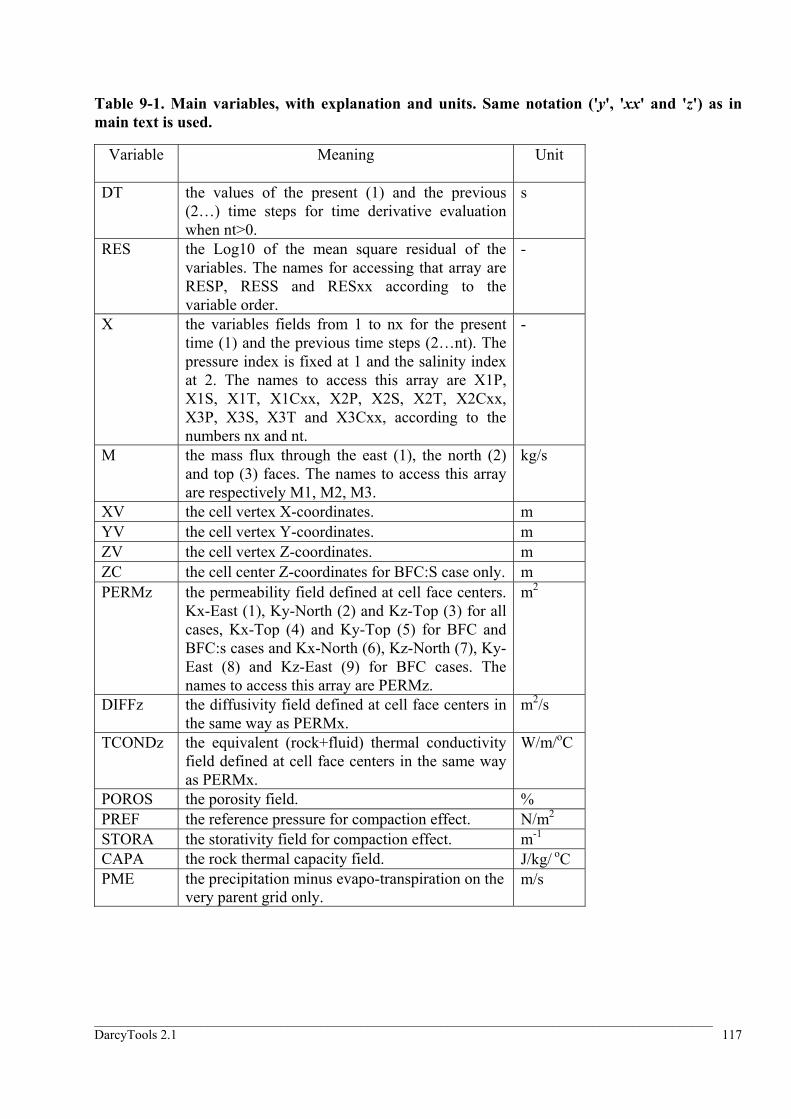
_____________________________________________________________________________________________ DarcyTools 2.1 117
Table 9-1. Main variables, with explanation and units. Same notation ('y', 'xx' and 'z') as in main text is used.
Variable Meaning Unit
DT the values of the present (1) and the previous (2…) time steps for time derivative evaluation when nt>0.
s
RES the Log10 of the mean square residual of the variables. The names for accessing that array are RESP, RESS and RESxx according to the variable order.
-
X the variables fields from 1 to nx for the present time (1) and the previous time steps (2…nt). The pressure index is fixed at 1 and the salinity index at 2. The names to access this array are X1P, X1S, X1T, X1Cxx, X2P, X2S, X2T, X2Cxx, X3P, X3S, X3T and X3Cxx, according to the numbers nx and nt.
-
M the mass flux through the east (1), the north (2) and top (3) faces. The names to access this array are respectively M1, M2, M3.
kg/s
XV the cell vertex X-coordinates. m YV the cell vertex Y-coordinates. m ZV the cell vertex Z-coordinates. m ZC the cell center Z-coordinates for BFC:S case only. m PERMz the permeability field defined at cell face centers.
Kx-East (1), Ky-North (2) and Kz-Top (3) for all cases, Kx-Top (4) and Ky-Top (5) for BFC and BFC:s cases and Kx-North (6), Kz-North (7), Ky-East (8) and Kz-East (9) for BFC cases. The names to access this array are PERMz.
m2
DIFFz the diffusivity field defined at cell face centers in the same way as PERMx.
m2/s
TCONDz the equivalent (rock+fluid) thermal conductivity field defined at cell face centers in the same way as PERMx.
W/m/oC
POROS the porosity field. % PREF the reference pressure for compaction effect. N/m2 STORA the storativity field for compaction effect. m-1 CAPA the rock thermal capacity field. J/kg/ oC PME
the precipitation minus evapo-transpiration on the very parent grid only.
m/s

Appendix A User Subroutines

Contents
INTRODUCTION........................................................................................... 1
UTIL-SECTION........................................................................................... 1
LFNAME .........................................................................................1
LENAME .........................................................................................2
SET_xxxx.......................................................................................3
GET_xxxx ......................................................................................4
IUFREE ..........................................................................................5
IND_VAL........................................................................................5
IND_SET........................................................................................5
IND_GET........................................................................................6
USR ROUTINES .......................................................................................... 6
USRSET .........................................................................................7
USRINI ..........................................................................................8
USRMESH ......................................................................................8
USRDT.........................................................................................10
USRBOSS.....................................................................................10
USRPROP .....................................................................................11
USRSLV .......................................................................................12
USROUT.......................................................................................12
USRPRECO ...................................................................................13
MIGAL ROUTINES .................................................................................... 13
SETRELAX ....................................................................................14
SETDOMI .....................................................................................14
GEOM ROUTINES...................................................................................... 15
MESH_P.......................................................................................15
MESH_R.......................................................................................16

Contents___________________________________________________________________
DarcyTools 2.1
MESH_W......................................................................................16
IZN1 ...........................................................................................17
IZN2 ...........................................................................................17
IZN3 ...........................................................................................18
IZN4 ...........................................................................................18
IXDIST ........................................................................................19
IZDIST ........................................................................................20
DTDIST........................................................................................21
TEC ROUTINES ......................................................................................... 22
TEC_INI.......................................................................................23
TEC_ZNE .....................................................................................24
TEC_BLK......................................................................................25
TEC_END .....................................................................................25
Example program..........................................................................26
ROF ROUTINES ........................................................................................ 28
ROF_INI ......................................................................................29
ROF_GRD.....................................................................................29
ROF_TIM......................................................................................30
ROF_NAM.....................................................................................30
ROF_VAL......................................................................................31
Example program..........................................................................31
User subroutines Introduction
DarcyTools 2.1 1
User subroutines
Introduction
In order to provide users with programming capabilities the DarcyTools solver
automatically calls some template subroutines named user’s routines. All those
routines are gathered into the User-Section and are initially empty. Depending
on the case to run, users will be able to program one or several routines of this
section.
The kernel of the setting is located into USRSET and is called at the beginning of
each run. To support users in programming this routine, and because of the
interdependence between some of the parameters, a Set-Section has been
created that contains many routines dedicated to the parameters setting.
Several users’ routines are also called during the run to provide users with a
certain level of control on the computation. Those routines allow overwriting the
initial parameters, the properties or the outputs.
UTIL-section
In order to help users with internal programming and data organization (i.e.
with F array handling) a Util-Section gathers some utility routines that users
should use for safely programming the User-Section routines.
LFNAME
This routine returns the F array index of the first element of the sub-array
named ‘name’ on the grid igrd. It allows user to safely access the any sub-array

User subroutines UTIL-section
DarcyTools 2.1 2
independently of the solver internal data ordering. It also applies to user’s data
defined by routine SETARRAY. When the sub-array is not defined on the given
grid this routine returns 0.
*======================================================================* * * * function lfname(name,igrd) * * * *======================================================================* *F90 * * * * INPUT * * ----- * * name ......... array or user's variable name * * igrd ......... grid index * * * *======================================================================*
LENAME
This routine returns the length of the F sub-array named ‘name’ on the grid igrd.
In conjunction with the LFNAME routine it allows user to safely access the any
sub-array independently of the solver internal data ordering. For example, the
good practice for setting a property should be:
subroutine usrxxx(f,igrd,ni,nj,nk,...) dimension f(*) lstora = lfname(‘STORA’,igrd) nstora = lename(‘STORA’,igrd) if(nstora.eq.1) then f(lstora) = value elseif(nstora.eq.ni*nj*nk) then do i=1,ni do j=1,nj do k=1,nk l = (i-1) + (j-1)*ni + (k-1)*ni*nj f(lstora+l) = val(i,j,k) enddo enddo enddo else print *,’STORA is undefined on this grid’ return endif . . . end

User subroutines UTIL-section
DarcyTools 2.1 3
When the sub-array is not defined on the given grid this routine returns 0.
*======================================================================* * * * function lename(name,igrd) * * * *======================================================================* *F90 * * * * INPUT * * ----- * * name ......... array or user's variable name * * igrd ......... grid index * * * *======================================================================*
SET_xxxx
In order to save memory storage, users can store uniform properties into single
element arrays instead of 3D arrays by calling the routine SETF0. Hence to free
users from checking the array length when accessing properties the Util-Section
implements routines with the pattern SET_xxxx where xxxx represents the
property name (SET_POROS, SET_STORA, SET_PREF, SET_CAPA, SET_TCONDx,
SET_PERMx, SET_DIFFx). For example, the good practice for setting a property
could also be:
subroutine usrxxx(f,igrd,ni,nj,nk,...) dimension f(*) do i=1,ni do j=1,nj do k=1,nk call set_stora(i,j,k,igrd,val(i,j,k)) enddo enddo enddo . . . end
*======================================================================* * * * subroutine set_xxxx(i,j,k,igrd,value) * * * *======================================================================* * F90 * * * * INPUT * * ----- * * i,j,k ........ cell indexes * * igrd ......... grid index * * value ........ value to set * * * *======================================================================*

User subroutines UTIL-section
DarcyTools 2.1 4
GET_xxxx
Like the routines SET_xxxx set properties values independently of the length of
the corresponding sub-array length, the GET_xxxx functions retrieve the
properties value of the cell (i,j,k) of the grid igrd. The name of those functions
follows the pattern GET_xxxx where xxxx represents the property name
(GET_POROS, GET_STORA, GET_PREF, GET_CAPA, GET_TCOND, GET_PERM,
GET_DIFF). For example, the good practice for getting a property could be:
subroutine usrxxx(f,igrd,ni,nj,nk,...) dimension f(*) do i=1,ni do j=1,nj do k=1,nk value(i,j,k) = get_stora(i,j,k,igrd) enddo enddo enddo . . . end
*======================================================================* * * * function get_xxxx(i,j,k,igrd) * * * *======================================================================* * F90 * * * * INPUT * * ----- * * i,j,k ........ cell indexes * * igrd ......... grid index * * * *======================================================================*
When properties such as the conductivity, the permeability or the diffusivity
fields are four dimensional array, the GET_xxxx function uses one argument
more; namely the fourth index in the array (the x value of the names TCONDx,
PERMx or DIFFx). In such a case the GET_xxxx function becomes.
*======================================================================* * * * function get_xxxx(i,j,k,igrd,lval) * * * *======================================================================* * F90 * * * * INPUT * * ----- * * i,j,k ........ cell indexes * * igrd ......... grid index * * lval ......... xxxx fourth index * * * *======================================================================*
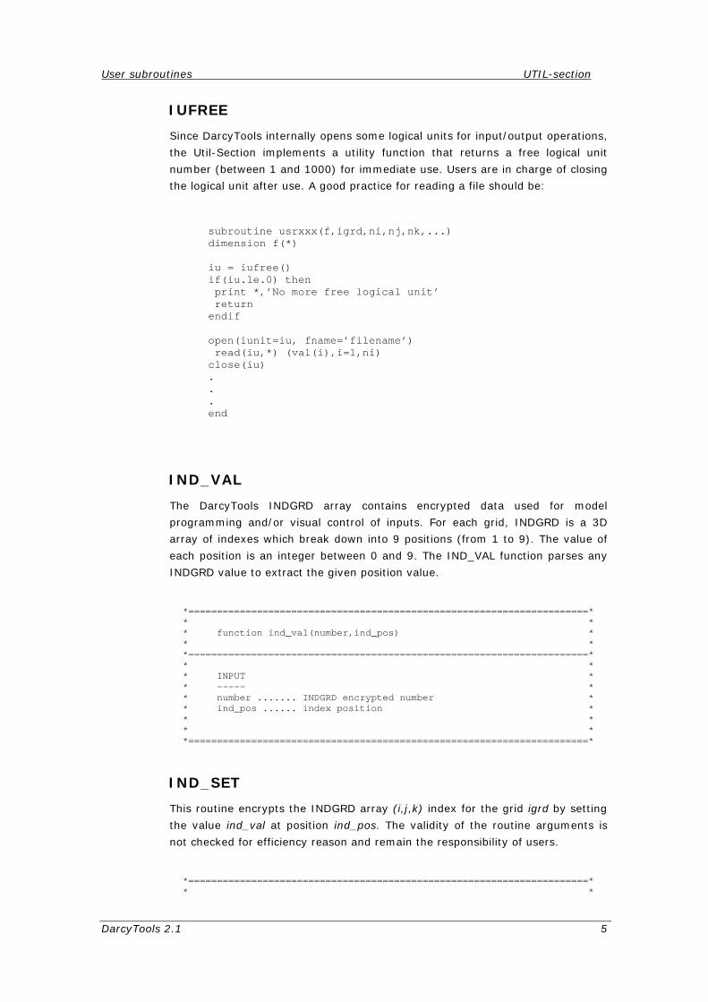
User subroutines UTIL-section
DarcyTools 2.1 5
IUFREE
Since DarcyTools internally opens some logical units for input/output operations,
the Util-Section implements a utility function that returns a free logical unit
number (between 1 and 1000) for immediate use. Users are in charge of closing
the logical unit after use. A good practice for reading a file should be:
subroutine usrxxx(f,igrd,ni,nj,nk,...) dimension f(*) iu = iufree() if(iu.le.0) then print *,’No more free logical unit’ return endif open(iunit=iu, fname=’filename’) read(iu,*) (val(i),i=1,ni) close(iu) . . . end
IND_VAL
The DarcyTools INDGRD array contains encrypted data used for model
programming and/or visual control of inputs. For each grid, INDGRD is a 3D
array of indexes which break down into 9 positions (from 1 to 9). The value of
each position is an integer between 0 and 9. The IND_VAL function parses any
INDGRD value to extract the given position value.
*======================================================================* * * * function ind_val(number,ind_pos) * * * *======================================================================* * * * INPUT * * ----- * * number ....... INDGRD encrypted number * * ind_pos ...... index position * * * * * *======================================================================*
IND_SET
This routine encrypts the INDGRD array (i,j,k) index for the grid igrd by setting
the value ind_val at position ind_pos. The validity of the routine arguments is
not checked for efficiency reason and remain the responsibility of users.
*======================================================================* * *
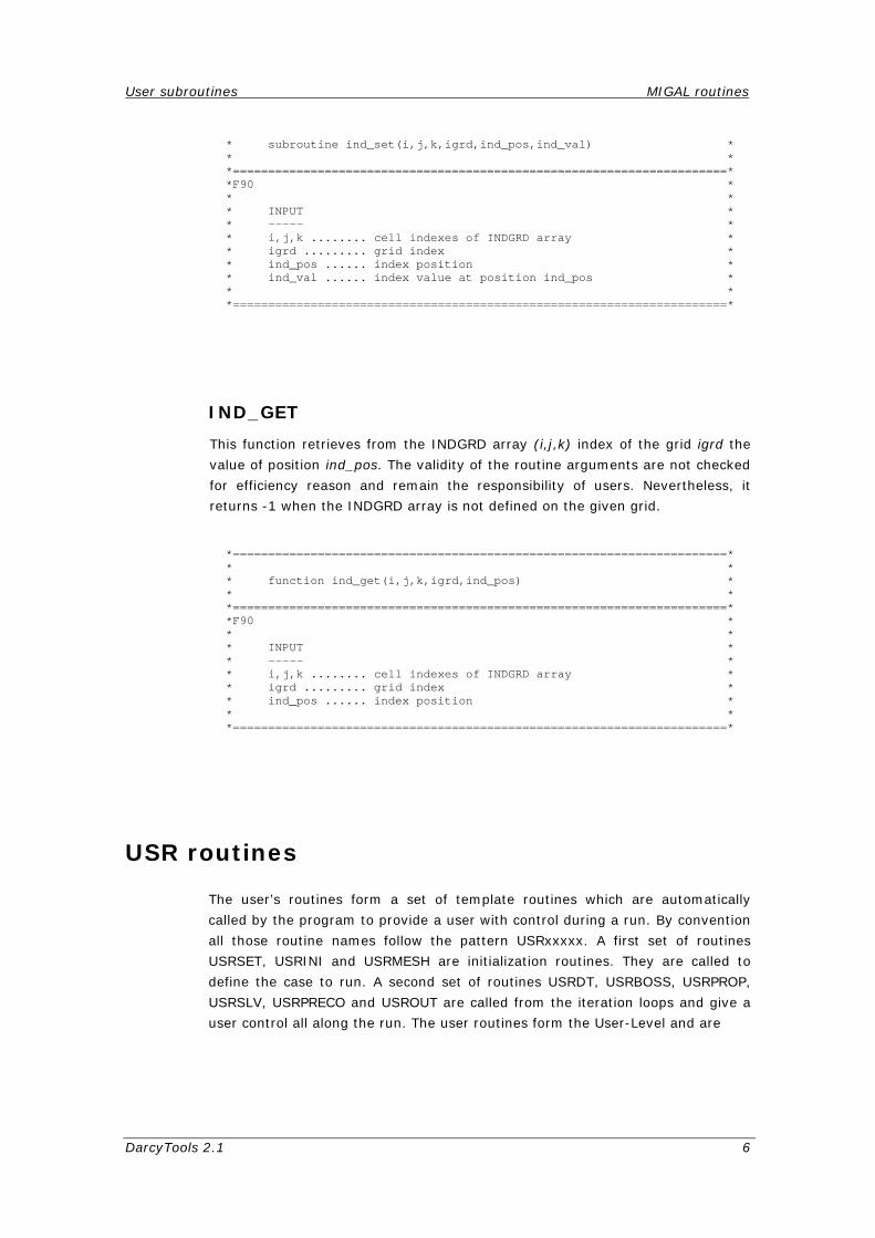
User subroutines MIGAL routines
DarcyTools 2.1 6
* subroutine ind_set(i,j,k,igrd,ind_pos,ind_val) * * * *======================================================================* *F90 * * * * INPUT * * ----- * * i,j,k ........ cell indexes of INDGRD array * * igrd ......... grid index * * ind_pos ...... index position * * ind_val ...... index value at position ind_pos * * * *======================================================================*
IND_GET
This function retrieves from the INDGRD array (i,j,k) index of the grid igrd the
value of position ind_pos. The validity of the routine arguments are not checked
for efficiency reason and remain the responsibility of users. Nevertheless, it
returns -1 when the INDGRD array is not defined on the given grid.
*======================================================================* * * * function ind_get(i,j,k,igrd,ind_pos) * * * *======================================================================* *F90 * * * * INPUT * * ----- * * i,j,k ........ cell indexes of INDGRD array * * igrd ......... grid index * * ind_pos ...... index position * * * *======================================================================*
USR routines
The user’s routines form a set of template routines which are automatically
called by the program to provide a user with control during a run. By convention
all those routine names follow the pattern USRxxxxx. A first set of routines
USRSET, USRINI and USRMESH are initialization routines. They are called to
define the case to run. A second set of routines USRDT, USRBOSS, USRPROP,
USRSLV, USRPRECO and USROUT are called from the iteration loops and give a
user control all along the run. The user routines form the User-Level and are

User subroutines MIGAL routines
DarcyTools 2.1 7
initially empty. They only need to be programmed when necessary, according to
their calling sequence.
default setting CIF setting USRSET USRMEH USRINI do istep = 1, nstep USRDT do itg = 1, nitg do igrd = lgrd,1,-1 do sweep = 1, nsweep do ivar = nvar1, nvar2 USRPROP build operator USRBOSS if coupled USRPRECO USRSLV solve operator USROUT enddo
do itc = 1, nitc1 do ivar = nvar3, nvar4
USRPROP build operator USRBOSS if coupled USRPRECO USRSLV solve operator USROUT enddo enddo enddo
do itc = 1, nitc2 do ivar = nvar5, nvar6 USRPROP build operator USRBOSS if coupled USRPRECO USRSLV solve operator USROUT enddo enddo enddo enddo enddo
Figure 1: User’s routines calling sequence
USRSET
This routine is the first user’s routine called after the installation of the default
setting by the main program. It is where users must define and specify the

User subroutines MIGAL routines
DarcyTools 2.1 8
parameters of the case to run by calling several setting’s routines of the Set-
Section. This routine is called once and only once so that it is also the right place
to declare and allocate user’s arrays.
*======================================================================* * * * subroutine usrset() * * * *======================================================================*
USRINI
This routine is called after USRSET and USRMESH, and before starting the
integration loops. It is called by the routine SETINI and dedicated to
initialization. It is the place where users should overwrite the NULL field default
initialization of variables. Only the previous time steps variables need to be
defined here (e.g. X2P, X3P…). The current time step initial estimation is
automatically set to the previous time step solution by the routine SETINI.
*======================================================================* * * * subroutine usrini(igrd,icos,f,ni,nj,nk,nx,nt) * * * *======================================================================* * * * INPUT * * ----- * * * * igrd ....... grid index * * icos ....... kind of grid (1=BFC, 2=BFC:s, 3=CART) * * f .......... farray * * ni ......... number of cells in the direction x * * nj ......... number of cells in the direction y * * nk ......... number of cells in the direction z * * nx ......... number of variables in the X sub-array * * nt ......... number of time steps in the X sub-array * * * * * * OUPUT * * ----- * * * * x .......... X past values (i,j,k,n,2...) * * * *======================================================================*
USRMESH
This routine is automatically called from SETINI/SETMESH after the user
settings. Its programming is necessary to define the grid vertex coordinates and
to overwrite the default uniform Cartesian grid. These coordinates can be read
from a file or computed in the routine. This routine is not called for embedded
grids. The embedded grids are automatically interpolated from their parent grid

User subroutines MIGAL routines
DarcyTools 2.1 9
by the routine EMBMESHx of Geom-Section. Therefore, if the embedded grids
are needed outside of the DarcyTools solver, for example to define the property
fields, users should use the same EMBMESHx routines to compute them.
Because of the node-centered approach of the code, the control volumes are
defined by grid cells and the number of vertexes in each direction equals the
number of cells plus one. Depending on the coordinate system (icos) employed
a good practice for coordinate access could be:
subroutine usrmesh(igrd,icos,f,igrd,ni,nj,nk,nx,nt) dimension f(*) lzv = lfname(‘ZV’,igrd) if(icos.eq.3) then do k=1,nk+1 f(lzv+k-1) = zv1(k) enddo else do i=1,ni+1 do j=1,nj+1 do k=1,nk+1 l = (i-1) + (j-1)*(ni+1) + (k-1)*(ni+1)*(nj+1) f(lzv+l) = zv3(i,j,k) enddo enddo enddo endif . . . end
*======================================================================* * * * subroutine usrmesh(igrd,icos,f,ni,nj,nk,nx,nt) * * * *======================================================================* * * * INPUT * * ----- * * * * igrd ....... grid index * * icos ....... kind of grid (1=BFC, 2=BFC:s, 3=CART) * * f .......... farray * * ni ......... number of cells in the direction x * * nj ......... number of cells in the direction y * * nk ......... number of cells in the direction z * * nx ......... number of variables in the X sub-array * * nt ......... number of time steps in the X sub-array * * * * * * OUPUT * * ----- * * * * xv ......... new x-coordinates of grid nodes * * yv ......... new y-coordinates of grid nodes * * zv ......... new z-coordinates of grid nodes * * * *======================================================================*
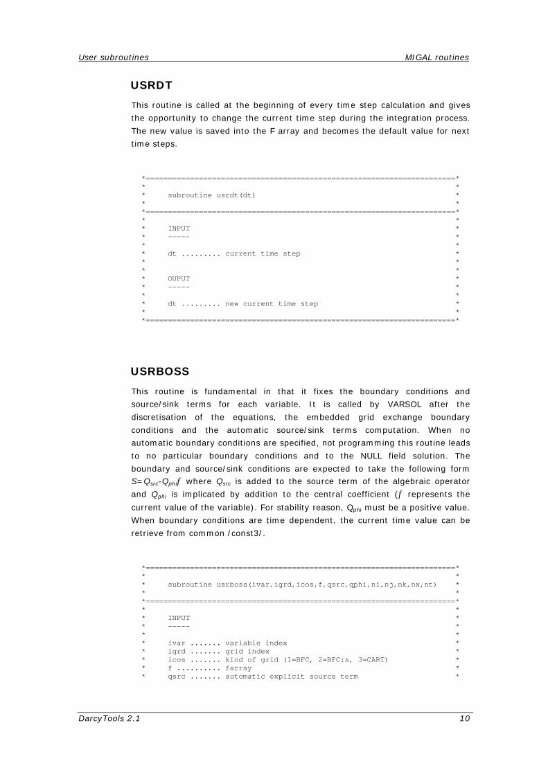
User subroutines MIGAL routines
DarcyTools 2.1 10
USRDT
This routine is called at the beginning of every time step calculation and gives
the opportunity to change the current time step during the integration process.
The new value is saved into the F array and becomes the default value for next
time steps.
*======================================================================* * * * subroutine usrdt(dt) * * * *======================================================================* * * * INPUT * * ----- * * * * dt ......... current time step * * * * * * OUPUT * * ----- * * * * dt ......... new current time step * * * *======================================================================*
USRBOSS
This routine is fundamental in that it fixes the boundary conditions and
source/sink terms for each variable. It is called by VARSOL after the
discretisation of the equations, the embedded grid exchange boundary
conditions and the automatic source/sink terms computation. When no
automatic boundary conditions are specified, not programming this routine leads
to no particular boundary conditions and to the NULL field solution. The
boundary and source/sink conditions are expected to take the following form S=Qsrc-Qphiφ where Qsrc is added to the source term of the algebraic operator
and Qphi is implicated by addition to the central coefficient (φ represents the
current value of the variable). For stability reason, Qphi must be a positive value.
When boundary conditions are time dependent, the current time value can be
retrieve from common /const3/.
*======================================================================* * * * subroutine usrboss(ivar,igrd,icos,f,qsrc,qphi,ni,nj,nk,nx,nt) * * * *======================================================================* * * * INPUT * * ----- * * * * ivar ....... variable index * * igrd ....... grid index * * icos ....... kind of grid (1=BFC, 2=BFC:s, 3=CART) * * f .......... farray * * qsrc ....... automatic explicit source term *
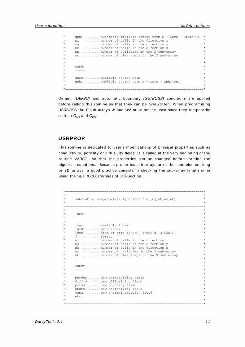
User subroutines MIGAL routines
DarcyTools 2.1 11
* qphi ....... automatic implicit source term S = Qsrc - Qphi*PHI * * ni ......... number of cells in the direction x * * nj ......... number of cells in the direction y * * nk ......... number of cells in the direction z * * nx ......... number of variables in the X sub-array * * nt ......... number of time steps in the X sub-array * * * * * * OUPUT * * ----- * * * * qsrc ....... explicit source term * * qphi ....... implicit source term S = Qsrc - Qphi*PHI * * * *======================================================================*
Default (DEFBC) and automatic boundary (SETBOSS) conditions are applied
before calling this routine so that they can be overwritten. When programming
USRBOSS the F sub-arrays W and W2 must not be used since they temporarily
contain Qsrc and Qphi.
USRPROP
This routine is dedicated to user’s modifications of physical properties such as
conductivity, porosity or diffusivity fields. It is called at the very beginning of the
routine VARSOL so that the properties can be changed before forming the
algebraic equations. Because properties sub arrays are either one element long
or 3D arrays, a good practice consists in checking the sub-array length or in
using the SET_XXXX routines of Util-Section.
*======================================================================* * * * subroutine usrprop(ivar,igrd,icos,f,ni,nj,nk,nx,nt) * * * *======================================================================* * * * INPUT * * ----- * * * * ivar ....... variable index * * igrd ....... grid index * * icos ....... kind of grid (1=BFC, 2=BFC:s, 3=CART) * * f .......... farray * * ni ......... number of cells in the direction x * * nj ......... number of cells in the direction y * * nk ......... number of cells in the direction z * * nx ......... number of variables in the X sub-array * * nt ......... number of time steps in the X sub-array * * * * * * OUPUT * * ----- * * * * permea ..... new permeability field * * diffco ..... new diffusivity field * * poros ...... new porosity field * * stora ...... new storativity field * * capa ....... new thermal capacity field * * etc. * * * *======================================================================*
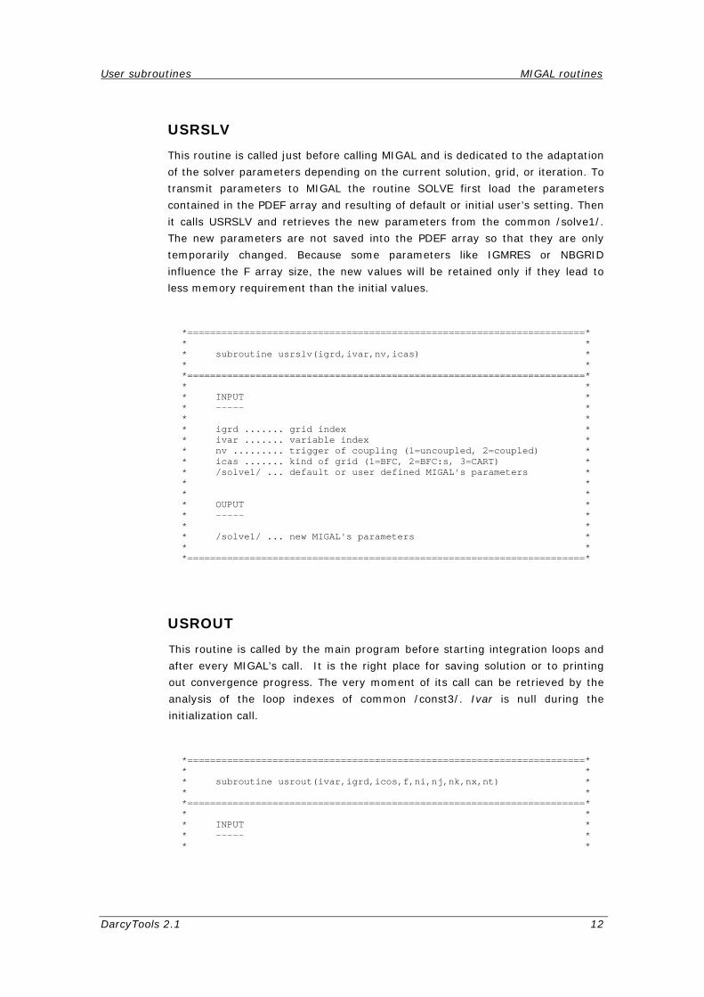
User subroutines MIGAL routines
DarcyTools 2.1 12
USRSLV
This routine is called just before calling MIGAL and is dedicated to the adaptation
of the solver parameters depending on the current solution, grid, or iteration. To
transmit parameters to MIGAL the routine SOLVE first load the parameters
contained in the PDEF array and resulting of default or initial user’s setting. Then
it calls USRSLV and retrieves the new parameters from the common /solve1/.
The new parameters are not saved into the PDEF array so that they are only
temporarily changed. Because some parameters like IGMRES or NBGRID
influence the F array size, the new values will be retained only if they lead to
less memory requirement than the initial values.
*======================================================================* * * * subroutine usrslv(igrd,ivar,nv,icas) * * * *======================================================================* * * * INPUT * * ----- * * * * igrd ....... grid index * * ivar ....... variable index * * nv ......... trigger of coupling (1=uncoupled, 2=coupled) * * icas ....... kind of grid (1=BFC, 2=BFC:s, 3=CART) * * /solve1/ ... default or user defined MIGAL's parameters * * * * * * OUPUT * * ----- * * * * /solve1/ ... new MIGAL's parameters * * * *======================================================================*
USROUT
This routine is called by the main program before starting integration loops and
after every MIGAL’s call. It is the right place for saving solution or to printing
out convergence progress. The very moment of its call can be retrieved by the
analysis of the loop indexes of common /const3/. Ivar is null during the
initialization call.
*======================================================================* * * * subroutine usrout(ivar,igrd,icos,f,ni,nj,nk,nx,nt) * * * *======================================================================* * * * INPUT * * ----- * * *
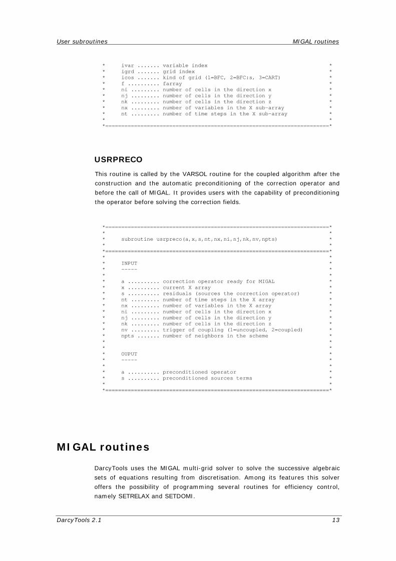
User subroutines MIGAL routines
DarcyTools 2.1 13
* ivar ....... variable index * * igrd ....... grid index * * icos ....... kind of grid (1=BFC, 2=BFC:s, 3=CART) * * f .......... farray * * ni ......... number of cells in the direction x * * nj ......... number of cells in the direction y * * nk ......... number of cells in the direction z * * nx ......... number of variables in the X sub-array * * nt ......... number of time steps in the X sub-array * * * *======================================================================*
USRPRECO
This routine is called by the VARSOL routine for the coupled algorithm after the
construction and the automatic preconditioning of the correction operator and
before the call of MIGAL. It provides users with the capability of preconditioning
the operator before solving the correction fields.
*======================================================================* * * * subroutine usrpreco(a,x,s,nt,nx,ni,nj,nk,nv,npts) * * * *======================================================================* * * * INPUT * * ----- * * * * a .......... correction operator ready for MIGAL * * x .......... current X array * * s .......... residuals (sources the correction operator) * * nt ......... number of time steps in the X array * * nx ......... number of variables in the X array * * ni ......... number of cells in the direction x * * nj ......... number of cells in the direction y * * nk ......... number of cells in the direction z * * nv ......... trigger of coupling (1=uncoupled, 2=coupled) * * npts ....... number of neighbors in the scheme * * * * * * OUPUT * * ----- * * * * a .......... preconditioned operator * * s .......... preconditioned sources terms * * * *======================================================================*
MIGAL routines
DarcyTools uses the MIGAL multi-grid solver to solve the successive algebraic
sets of equations resulting from discretisation. Among its features this solver
offers the possibility of programming several routines for efficiency control,
namely SETRELAX and SETDOMI.
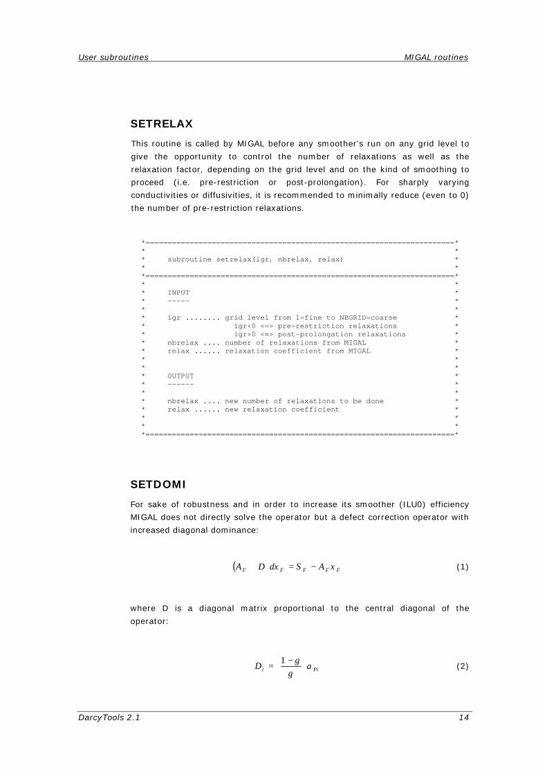
User subroutines MIGAL routines
DarcyTools 2.1 14
SETRELAX
This routine is called by MIGAL before any smoother’s run on any grid level to
give the opportunity to control the number of relaxations as well as the
relaxation factor, depending on the grid level and on the kind of smoothing to
proceed (i.e. pre-restriction or post-prolongation). For sharply varying
conductivities or diffusivities, it is recommended to minimally reduce (even to 0)
the number of pre-restriction relaxations.
*======================================================================* * * * subroutine setrelax(igr, nbrelax, relax) * * * *======================================================================* * * * INPUT * * ----- * * * * igr ........ grid level from 1=fine to NBGRID=coarse * * igr<0 <=> pre-restriction relaxations * * igr>0 <=> post-prolongation relaxations * * nbrelax .... number of relaxations from MIGAL * * relax ...... relaxation coefficient from MIGAL * * * * * * OUTPUT * * ------ * * * * nbrelax .... new number of relaxations to be done * * relax ...... new relaxation coefficient * * * * * *======================================================================*
SETDOMI
For sake of robustness and in order to increase its smoother (ILU0) efficiency
MIGAL does not directly solve the operator but a defect correction operator with
increased diagonal dominance:
( ) FFFFF xASxDA −=+ δ (1)
where D is a diagonal matrix proportional to the central diagonal of the
operator:
Pii aD
−=
γγ1
(2)
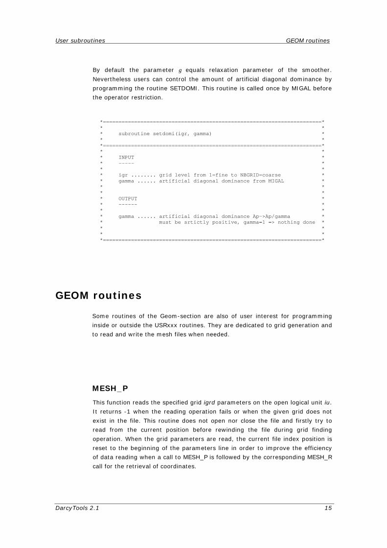
User subroutines GEOM routines
DarcyTools 2.1 15
By default the parameter γ equals relaxation parameter of the smoother.
Nevertheless users can control the amount of artificial diagonal dominance by
programming the routine SETDOMI. This routine is called once by MIGAL before
the operator restriction.
*======================================================================* * * * subroutine setdomi(igr, gamma) * * * *======================================================================* * * * INPUT * * ----- * * * * igr ........ grid level from 1=fine to NBGRID=coarse * * gamma ...... artificial diagonal dominance from MIGAL * * * * * * OUTPUT * * ------ * * * * gamma ...... artificial diagonal dominance Ap->Ap/gamma * * must be srtictly positive, gamma=1 => nothing done * * * * * *======================================================================*
GEOM routines
Some routines of the Geom-section are also of user interest for programming
inside or outside the USRxxx routines. They are dedicated to grid generation and
to read and write the mesh files when needed.
MESH_P
This function reads the specified grid igrd parameters on the open logical unit iu.
It returns -1 when the reading operation fails or when the given grid does not
exist in the file. This routine does not open nor close the file and firstly try to
read from the current position before rewinding the file during grid finding
operation. When the grid parameters are read, the current file index position is
reset to the beginning of the parameters line in order to improve the efficiency
of data reading when a call to MESH_P is followed by the corresponding MESH_R
call for the retrieval of coordinates.

User subroutines GEOM routines
DarcyTools 2.1 16
*======================================================================* * * * function mesh_p(iu,igrd, ni,nj,nk,icos,ip,i1,i2,j1,j2,k1,k2) * * * *======================================================================* * * * INPUT * * ----- * * iu ........... open logical unit on grid file (unformatted) * * igrd ......... grid index * * * * * * OUTPUT * * ------ * * ni,nj,nk ..... number of cells per direction * * icos ......... kind of grid 1=BFC, 2=BFC:s, 3=CART * * ip ........... parent grid index * * i1,i2,.,k2 ... footprint on parent grid * * mesh_p ....... reading status 0 = ok * * -1 = error * * * *======================================================================*
MESH_R
This function reads the specified grid igrd on the open logical unit iu and fills the
cell vertex coordinates arrays Xv, Yv and Zv. It returns -1 when the reading
operation fails or when the given grid does not exist in the file. This routine does
not open nor close the file and firstly try to read from the current position before
rewinding the file during grid finding operation. No dimension checking is
performed on the coordinate arrays. Hence users are in charge of the proper
allocation e.g. by calling MESH_P before.
*======================================================================* * * * function mesh_r(iu,igrd,xv,yv,zv) * * * *======================================================================* * * * INPUT * * ----- * * iu ........... open logical unit on grid file (unformatted) * * igrd ......... grid index * * * * * * OUTPUT * * ------ * * xv,yv,zv ..... coordinates arrays * * mesh_r ....... reading status 0 = ok * * -1 = error * * * *======================================================================*
MESH_W
This function writes the specified grid igrd cell vertex coordinates arrays Xv, Yv
and Zv on the open logical unit iu. It returns -1 when the writing operation
fails. This routine does not open nor close the file.
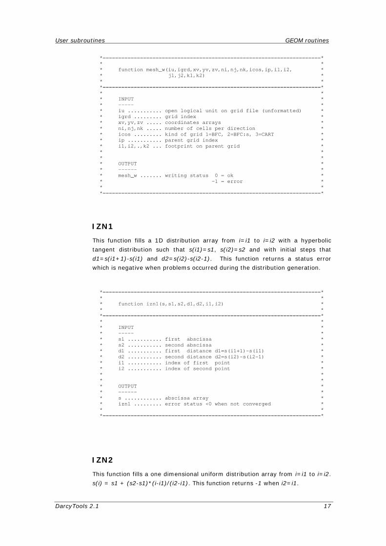
User subroutines GEOM routines
DarcyTools 2.1 17
*======================================================================* * * * function mesh_w(iu,igrd,xv,yv,zv,ni,nj,nk,icos,ip,i1,i2, * * j1,j2,k1,k2) * * * *======================================================================* * * * INPUT * * ----- * * iu ........... open logical unit on grid file (unformatted) * * igrd ......... grid index * * xv,yv,zv ..... coordinates arrays * * ni,nj,nk ..... number of cells per direction * * icos ......... kind of grid 1=BFC, 2=BFC:s, 3=CART * * ip ........... parent grid index * * i1,i2,.,k2 ... footprint on parent grid * * * * * * OUTPUT * * ------ * * mesh_w ....... writing status 0 = ok * * -1 = error * * * *======================================================================*
IZN1
This function fills a 1D distribution array from i=i1 to i=i2 with a hyperbolic
tangent distribution such that s(i1)=s1, s(i2)=s2 and with initial steps that
d1=s(i1+1)-s(i1) and d2=s(i2)-s(i2-1). This function returns a status error
which is negative when problems occurred during the distribution generation.
*======================================================================* * * * function izn1(s,s1,s2,d1,d2,i1,i2) * * * *======================================================================* * * * INPUT * * ----- * * s1 ........... first abscissa * * s2 ........... second abscissa * * d1 ........... first distance d1=s(i1+1)-s(i1) * * d2 ........... second distance d2=s(i2)-s(i2-1) * * i1 ........... index of first point * * i2 ........... index of second point * * * * * * OUTPUT * * ------ * * s ............ abscissa array * * izn1 ......... error status <0 when not converged * * * *======================================================================*
IZN2
This function fills a one dimensional uniform distribution array from i=i1 to i=i2.
s(i) = s1 + (s2-s1)*(i-i1)/(i2-i1). This function returns -1 when i2=i1.
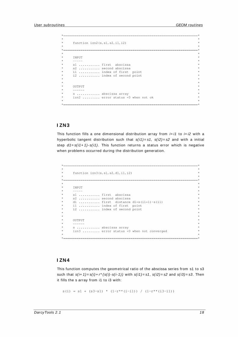
User subroutines GEOM routines
DarcyTools 2.1 18
*======================================================================* * * * function izn2(s,s1,s2,i1,i2) * * * *======================================================================* * * * INPUT * * ----- * * s1 ........... first abscissa * * s2 ........... second abscissa * * i1 ........... index of first point * * i2 ........... index of second point * * * * * * OUTPUT * * ------ * * s ............ abscissa array * * izn2 ......... error status <0 when not ok * * * *======================================================================*
IZN3
This function fills a one dimensional distribution array from i=i1 to i=i2 with a
hyperbolic tangent distribution such that s(i1)=s1, s(i2)=s2 and with a initial
step d1=s(i1+1)-s(i1). This function returns a status error which is negative
when problems occurred during the distribution generation.
*======================================================================* * * * function izn3(s,s1,s2,d1,i1,i2) * * * *======================================================================* * * * INPUT * * ----- * * s1 ........... first abscissa * * s2 ........... second abscissa * * d1 ........... first distance d1=s(i1+1)-s(i1) * * i1 ........... index of first point * * i2 ........... index of second point * * * * * * OUTPUT * * ------ * * s ............ abscissa array * * izn3 ......... error status <0 when not converged * * * *======================================================================*
IZN4
This function computes the geometrical ratio of the abscissa series from s1 to s3
such that s(i+1)=s(i)+r*(s(i)-s(i-1)) with s(i1)=s1, s(i2)=s2 and s(i3)=s3. Then
it fills the s array from i1 to i3 with:
s(i) = s1 + (s3-s1) * (1-r**(i-i1)) / (1-r**(i3-i1))

User subroutines GEOM routines
DarcyTools 2.1 19
*======================================================================* * * * function izn4(s,s1,s2,s3,i1,i2,i3) * * * *======================================================================* * * * INPUT * * ----- * * s1 ........... first abscissa * * s2 ........... second abscissa * * s3 ........... third abscissa * * i1 ........... index of first point * * i2 ........... index of second point * * i3 ........... index of third point * * * * * * OUTPUT * * ------ * * s ............ abscissa array * * izn4 ......... error status <0 when not converged * * * *======================================================================*
IXDIST
This routine fills a one dimensional distribution array following three zones. The
first zone sets a (hyperbolic) tangent distribution of n1 cells between x0 and x1.
The expansion (contraction) is computed to fit an n1+1 cell size d=(x2-x1)/n2.
When n2=0 the first zone is a uniform distribution zone. The second zone set n2
constant size cells between x1 and x2 when n1>0 and between x0 and x2 when
n1=0. The third zone is a (hyperbolic) tangent distribution of n3 cells between
x2 and x3 when n2>0. The expansion (contraction) is computed to fit an n1+n2
cell size d=(x2-x1)/n2. When n2=0 the third zone is a uniform distribution zone
between x1 and x3 if n1>0 or between x0 and x3 if n1=0.
*======================================================================* * * * function ixdist(x,x0,x1,x2,x3,n1,n2,n3) * * * *======================================================================* * * * INPUT * * ----- * * x0 ........... west abscissa (node 1) * * x1 ........... west abscissa of zone 2 (node n1+1) * * x2 ........... east abscissa of zone 2 (node n1+n2+1) * * x3 ........... east abscissa (node n1+n2+n3+1) * * n1 ........... number of cells in zone 1 * * n2 ........... number of cells in zone 2 * * n3 ........... number of cells in zone 3 * * * * * * OUTPUT * * ------ * * x ............ coordinate array * * ixdist ....... error status =0 when ok * * * *======================================================================*

User subroutines GEOM routines
DarcyTools 2.1 20
IZDIST
This routine fills a one dimensional Zvij(k) distribution array following four zones.
The first zone sets a user distribution of n1 cells from top by cell sizes d1 i.e.
d1(i)=z(n-i+1)-z(n-i) with n=n1+n2+n3+n4. The second zone sets a
(hyperbolic) tangent distribution of n2 cells between z(n-n1+1) and z2. The
expansion (contraction) is computed to fit the n-n1+1 cell size and an n-n1-n2
cell size d=(z2-z3)/n3 when n3>0 or d=(z2-z4)/n4 when n3=0 and n4>0. When
n1=0 or n3=n4=0 the expansion (contraction) is only one side constraint and
when n1=n3=n4=0 the distribution is uniform between z0 and z2. The third
zone is a uniform cell spacing zone of n3 cells between z(n-n2-n1+1) and z3.
The fourth zone sets a (hyperbolic) tangent distribution of n4 cells between
z(n-n1-n2-n3+1) and z4. The expansion (contraction) is computed to fit the
n-n1-n2-n3+1 cell size when n1+n2+n3>0. The fourth zone is uniformly
spanned between z0 and z4 when n1=n2=n3=0.
Figure 2 : IZDIST zone labelling
This function returns a status error which is negative when problems occurred
during the distribution generation.
*======================================================================* * * * function izdist(z,z0,n1,d1,n2,z2,n3,z3,n4,z4) * * * *======================================================================* * * * INPUT * * ----- * * z0 ........... top abscissa (node n1+n2+n3+n4+1) * * n1 ........... number of cells in zone 1 *
Zone 4
Zone 3
Zone 2
Zone 1 d1(k)
n1 cells
n2 cells
n3 cells
n4 cells
Z0(i,j) cells
Z2
Z4
X
Z
Z3
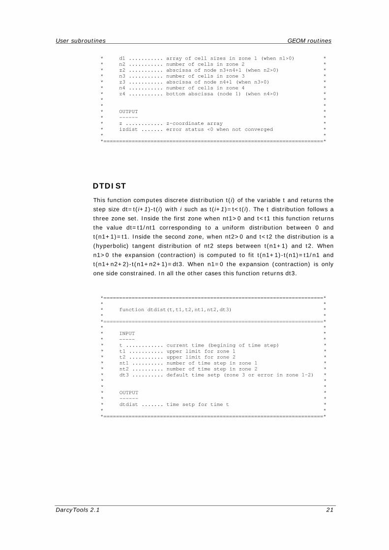
User subroutines GEOM routines
DarcyTools 2.1 21
* d1 ........... array of cell sizes in zone 1 (when n1>0) * * n2 ........... number of cells in zone 2 * * z2 ........... abscissa of node n3+n4+1 (when n2>0) * * n3 ........... number of cells in zone 3 * * z3 ........... abscissa of node n4+1 (when n3>0) * * n4 ........... number of cells in zone 4 * * z4 ........... bottom abscissa (node 1) (when n4>0) * * * * * * OUTPUT * * ------ * * z ............ z-coordinate array * * izdist ....... error status <0 when not converged * * * *======================================================================*
DTDIST
This function computes discrete distribution t(i) of the variable t and returns the
step size dt=t(i+1)-t(i) with i such as t(i+1)=t<t(i). The t distribution follows a
three zone set. Inside the first zone when nt1>0 and t<t1 this function returns
the value dt=t1/nt1 corresponding to a uniform distribution between 0 and
t(n1+1)=t1. Inside the second zone, when nt2>0 and t<t2 the distribution is a
(hyperbolic) tangent distribution of nt2 steps between t(n1+1) and t2. When
n1>0 the expansion (contraction) is computed to fit t(n1+1)-t(n1)=t1/n1 and
t(n1+n2+2)-t(n1+n2+1)=dt3. When n1=0 the expansion (contraction) is only
one side constrained. In all the other cases this function returns dt3.
*======================================================================* * * * function dtdist(t,t1,t2,nt1,nt2,dt3) * * * *======================================================================* * * * INPUT * * ----- * * t ............ current time (begining of time step) * * t1 ........... upper limit for zone 1 * * t2 ........... upper limit for zone 2 * * nt1 .......... number of time step in zone 1 * * nt2 .......... number of time step in zone 2 * * dt3 .......... default time setp (zone 3 or error in zone 1-2) * * * * * * OUTPUT * * ------ * * dtdist ....... time setp for time t * * * *======================================================================*
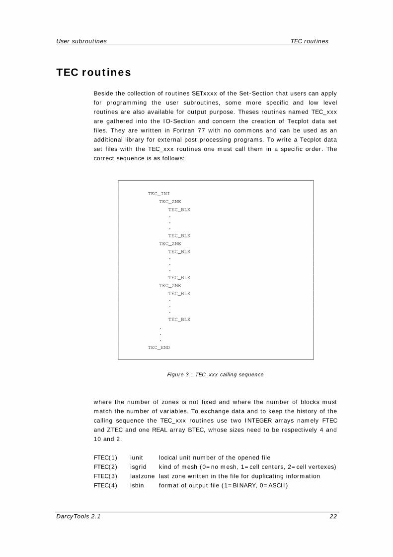
User subroutines TEC routines
DarcyTools 2.1 22
TEC routines
Beside the collection of routines SETxxxx of the Set-Section that users can apply
for programming the user subroutines, some more specific and low level
routines are also available for output purpose. Theses routines named TEC_xxx
are gathered into the IO-Section and concern the creation of Tecplot data set
files. They are written in Fortran 77 with no commons and can be used as an
additional library for external post processing programs. To write a Tecplot data
set files with the TEC_xxx routines one must call them in a specific order. The
correct sequence is as follows:
TEC_INI TEC_ZNE TEC_BLK . . . TEC_BLK TEC_ZNE TEC_BLK . . . TEC_BLK TEC_ZNE TEC_BLK . . . TEC_BLK . . . TEC_END
Figure 3 : TEC_xxx calling sequence
where the number of zones is not fixed and where the number of blocks must
match the number of variables. To exchange data and to keep the history of the
calling sequence the TEC_xxx routines use two INTEGER arrays namely FTEC
and ZTEC and one REAL array BTEC, whose sizes need to be respectively 4 and
10 and 2.
FTEC(1) iunit locical unit number of the opened file
FTEC(2) isgrid kind of mesh (0=no mesh, 1=cell centers, 2=cell vertexes)
FTEC(3) lastzone last zone written in the file for duplicating information
FTEC(4) isbin format of output file (1=BINARY, 0=ASCII)

User subroutines TEC routines
DarcyTools 2.1 23
ZTEC(1) nbcall counter for zone naming
ZTEC(2) i1 lower bound of the outputs in x direction
ZTEC(3) i2 upper bound of the outputs in x direction
ZTEC(4) ifr increment value of outputs in x direction
ZTEC(5) j1 lower bound of the outputs in y direction
ZTEC(6) j2 upper bound of the outputs in y direction
ZTEC(7) jfr increment value of the outputs in x direction
ZTEC(8) k1 lower bound of the outputs in z direction
ZTEC(9) k2 upper bound of the outputs in z direction
ZTEC(10) kfr increment value of outputs in z direction
BTEC(1) iaction kind of action to be performed on data before output
BTEC(2) vaction parameter of the specified action if any
FTEC(3) as well as ZTEC(1) are internally maintained by the calling sequence.
The former FTEC(3) doesn’t need to be set by users while the latter ZTEC(1)
should be initialize to 0.
The TEC_XXX routines call the TECXXX routines of the TECPLOT library when
binary option is selected. Hence, any program using the TEC_XXX routines, must
be linked either to the TECIO.LIB file (for windows) or to the TECIO.A file (for
linux). Moreover, for compatibility reason, the TEC_XXX routines include a
TECIO.FOR file provided with the TECPLOT package for windows. Under LINUX
the TECIO.FOR file must be an empty file.
TEC_INI
When FTEC(4)=0 this routine opens a new ASCII file, given a free logical unit
FTEC(1) and the file name fname. When FTEC(4)=1 this routine opens a new
binary TECPLOT file given the file name fname and return the file TECPLOT index
in FTEC(1). This routine also writes the title and variable names vlist strings in
the opened file. When FTEC(2) differs from 0 the “X Y Z” names are
automatically added first. The number of variables specified in the TEC_VAR
arguments will have to correspond exactly to the number of TEC_BLK calls in the
sequence. The file stays open during all the TEC_xxx calling sequence until
TEC_END. The last zone value FTEC(3) is initialized to 0.
*======================================================================* * * * subroutine tec_ini(ftec,fname,title,vlist,ierr) * * * *======================================================================* * * * INPUT * * ----- * * ftec ......... file parameters * * fname ........ name (including path) of the file to create *

User subroutines TEC routines
DarcyTools 2.1 24
* title ........ title of the data set (max 70 characters) * * vlist ........ list of variable names separated by space * * * * * * OUTPUT * * ------ * * ierr ......... error indicator (0 when successful) * * * *======================================================================*
TEC_ZNE
This routine first adds the TECPLOT zone statement to the data set. Then the
TECPLOT XYZ mesh is automatically added or declared DUPLICATE when izne
differs from FTEC(3). When FTEC(2)=1 the mesh is computed from xv, yv and
zv to be located at cell centers. When FTEC(2)=2 the mesh coincides with the
DarcyTools grid. Finally when FTEC(2)=0 no mesh is added after the zone
statement. ZTEC(1) is incremented by one in this routine.
*======================================================================* * * * subroutine tec_zne(izne,ftec,ztec,xv,yv,zv,w,ni,nj,nk,icos,ierr) * * * *======================================================================* * * * INPUT * * ----- * * izne ......... index of zone * * ftec ......... file parameters * * ztec ......... zone parameters * * xv,yv,zv ..... grid nodes coordinates * * w ............ work array at least (ni+1)*(nj+1)*(nk+1) long * * ni,nj,nk ..... number of cells in x,y and z directions * * icos ......... kind of grid (0=TRJ, 1=BFC, 2=BFC:s, 3=CART) * * * * * * OUTPUT * * ------ * * ierr ......... error indicator (0 if successful) * * * *======================================================================*
This routine automatically names the zone with the following pattern Zxxx-yyyy,
where xxx represents the zone index izne and where yyyy represents the
nbcall=ZTEC(1) value for the zone.
When ICOS=0 the routine writes a “trajectory” zone statement to the data set.
A trajectory statement is a I-ORDERED statement whose length is NI so that the
mesh becomes a line whose points coordinates are given by xv(i), yv(i) and zv(i)
with i=1 to i=ni. The trajectory zone statements are named following the
pattern TRJ-xxxxxx.
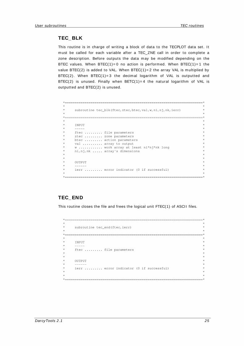
User subroutines TEC routines
DarcyTools 2.1 25
TEC_BLK
This routine is in charge of writing a block of data to the TECPLOT data set. It
must be called for each variable after a TEC_ZNE call in order to complete a
zone description. Before outputs the data may be modified depending on the
BTEC values. When BTEC(1)=0 no action is performed. When BTEC(1)=1 the
value BTEC(2) is added to VAL. When BTEC(1)=2 the array VAL is multiplied by
BTEC(2). When BTEC(1)=3 the decimal logarithm of VAL is outputted and
BTEC(2) is unused. Finally when BETC(1)=4 the natural logarithm of VAL is
outputted and BTEC(2) is unused.
*======================================================================* * * * subroutine tec_blk(ftec,ztec,btec,val,w,ni,nj,nk,ierr) * * * *======================================================================* * * * INPUT * * ----- * * ftec ......... file parameters * * ztec ......... zone parameters * * btec ......... action parameters * * val .......... array to output * * w ............ work array at least ni*nj*nk long * * ni,nj,nk ..... array's dimensions * * * * * * OUTPUT * * ------ * * ierr ......... error indicator (0 if successful) * * * *======================================================================*
TEC_END
This routine closes the file and frees the logical unit FTEC(1) of ASCII files.
*======================================================================* * * * subroutine tec_end(ftec,ierr) * * * *======================================================================* * * * INPUT * * ----- * * ftec ......... file parameters * * * * * * OUTPUT * * ------ * * ierr ......... error indicator (0 if successful) * * * * * *======================================================================*

User subroutines TEC routines
DarcyTools 2.1 26
Example program
This section lists an example program written in Fortran 77 which demonstrates
how to use of the TEC_xxx routines to write a Tecplot data set.
*======================================================================* *======================================================================* *======================================================================* *=========== ============* *=========== ============* *=========== DARCYTOOLS ============* *=========== ============* *=========== TEC writing sample ============* *=========== ============* *=========== ============* *======================================================================* *======================================================================* *======================================================================* * program writetec parameter (ni=10, nj=10, nk=10, nx=3, nt=10, ns=11*nx) character *(ns) sname integer ftec(4), ztec(10) dimension xv(ni+1), yv(nj+1), zv(nk+1), x(ni,nj,nk,nx,nt) dimension w(ni+1,nj+1,nk+1), btec(2) * prepare some data hx = 1. hy = 2. hz = 3. icos = 3 do i=1,ni+1 xv(i) = hx * (i-1) enddo do j=1,nj+1 yv(j) = hy * (j-1) enddo do k=1,nk+1 zv(k) = hz * (k-1) enddo do i=1,ni do j=1,nj do k=1,nk do l=1,nx do m=1,nt x(i,j,k,l,m) = i+j+k+l+m enddo enddo enddo enddo enddo * prepare the variable names string do i=1,nx j=1+(i-1)*11 write(sname(j:j+10),'(A5,I5.5,A1)') 'MyVar',i,' ' enddo * set the file unit ftec(1) = 15
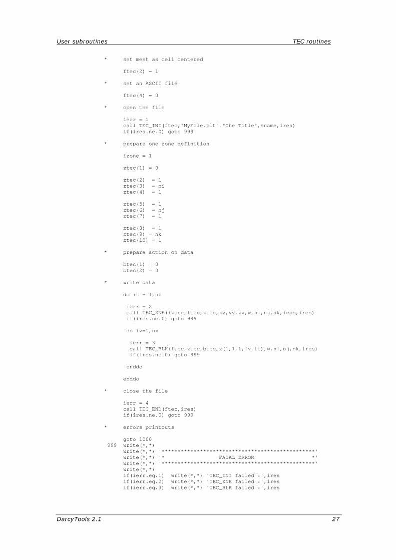
User subroutines TEC routines
DarcyTools 2.1 27
* set mesh as cell centered ftec(2) = 1 * set an ASCII file ftec(4) = 0 * open the file ierr = 1 call TEC_INI(ftec,"MyFile.plt","The Title",sname,ires) if(ires.ne.0) goto 999 * prepare one zone definition izone = 1 ztec(1) = 0 ztec(2) = 1 ztec(3) = ni ztec(4) = 1 ztec(5) = 1 ztec(6) = nj ztec(7) = 1 ztec(8) = 1 ztec(9) = nk ztec(10) = 1 * prepare action on data btec(1) = 0 btec(2) = 0 * write data do it = 1,nt ierr = 2 call TEC_ZNE(izone,ftec,ztec,xv,yv,zv,w,ni,nj,nk,icos,ires) if(ires.ne.0) goto 999 do iv=1,nx ierr = 3 call TEC_BLK(ftec,ztec,btec,x(1,1,1,iv,it),w,ni,nj,nk,ires) if(ires.ne.0) goto 999 enddo enddo * close the file ierr = 4 call TEC_END(ftec,ires) if(ires.ne.0) goto 999 * errors printouts goto 1000 999 write(*,*) write(*,*) '************************************************' write(*,*) '* FATAL ERROR *' write(*,*) '************************************************' write(*,*) if(ierr.eq.1) write(*,*) 'TEC_INI failed :',ires if(ierr.eq.2) write(*,*) 'TEC_ZNE failed :',ires if(ierr.eq.3) write(*,*) 'TEC_BLK failed :',ires
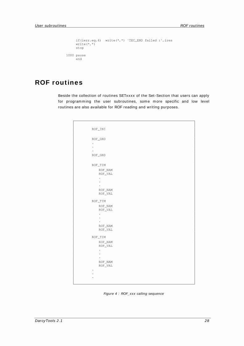
User subroutines ROF routines
DarcyTools 2.1 28
if(ierr.eq.4) write(*,*) 'TEC_END failed :',ires write(*,*) stop 1000 pause end
ROF routines
Beside the collection of routines SETxxxx of the Set-Section that users can apply
for programming the user subroutines, some more specific and low level
routines are also available for ROF reading and writing purposes.
ROF_INI ROF_GRD . . . ROF_GRD ROF_TIM ROF_NAM ROF_VAL . . . ROF_NAM ROF_VAL ROF_TIM ROF_NAM ROF_VAL . . . ROF_NAM ROF_VAL ROF_TIM ROF_NAM ROF_VAL . . . ROF_NAM ROF_VAL . . .
Figure 4 : ROF_xxx calling sequence

User subroutines ROF routines
DarcyTools 2.1 29
Theses routines named ROF_xxx are gathered into the IO-Section and concern
the data handling of the unformatted Result Output File (ROF). They are written
in Fortran 77 with no commons and can be used as an additional library for
external post processing programs. To read/write a ROF file with the ROF_xxx
routines one must call them in a specific order. The correct sequence is depicted
on Figure 4.
ROF_INI
This routine reads/writes the ROF header. This header tries to uniquely define
the DarcyTools run by the DarcyTools version number, the date and time of the
first execution, a title and the number of grids involved. This routine doesn’t
open the file but works on an unformatted file already open. The title is a 256
characters long string. The date is a 19 characters long string formatted as
follows “yyy-mm-dd hh:mm:ss”. The version is a 10 characters long string.
*======================================================================* * * * subroutine rof_ini(io,iu,ierr,title,date,version,lgrd) * * * *======================================================================* * * * INPUT * * ----- * * io ........... read/write switch (0=read, 1=write) * * iu ........... opened unformatted file unit * * title ........ title of the run (io=1) * * date ......... date of the run (io=1) * * version ...... DarcyTools version of the run (io=1) * * lgrd ......... number of grids (io=1) * * * * * * OUTPUT * * ------ * * ierr ......... error indicator (0 if successful) * * title ........ title of the run (io=0) * * date ......... date of the run (io=0) * * version ...... DarcyTools version of the run (io=0) * * lgrd ......... number of grids (io=0) * * * *======================================================================*
ROF_GRD
This routine reads/writes the grid definitions. A grid definition is an 11 integers
long array organized as follows: (ni, nj, nk, icas, ip, i1, i2, j1, j2, k1, k2).
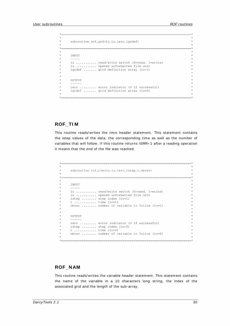
User subroutines ROF routines
DarcyTools 2.1 30
*======================================================================* * * * subroutine rof_grd(io,iu,ierr,igrdef) * * * *======================================================================* * * * INPUT * * ----- * * io ........... read/write switch (0=read, 1=write) * * iu ........... opened unformatted file unit * * igrdef ....... grid definition array (io=1) * * * * * * OUTPUT * * ------ * * ierr ......... error indicator (0 if successful) * * igrdef ....... grid definition array (io=0) * * * *======================================================================*
ROF_TIM
This routine reads/writes the time header statement. This statement contains
the istep values of the data, the corresponding time as well as the number of
variables that will follow. If this routine returns IERR=1 after a reading operation
it means that the end of the file was reached.
*======================================================================* * * * subroutine rof_tim(io,iu,ierr,istep,t,nbvar) * * * *======================================================================* * * * INPUT * * ----- * * io ........... read/write switch (0=read, 1=write) * * iu ........... opened unformatted file unit * * istep ........ step index (io=1) * * t ............ time (io=1) * * nbvar ........ number of variable to follow (io=1) * * * * * * OUTPUT * * ------ * * ierr ......... error indicator (0 if successful) * * istep ........ step index (io=0) * * t ............ time (io=0) * * nbvar ........ number of variable to follow (io=0) * * * *======================================================================*
ROF_NAM
This routine reads/writes the variable header statement. This statement contains
the name of the variable in a 10 characters long string, the index of the
associated grid and the length of the sub-array.
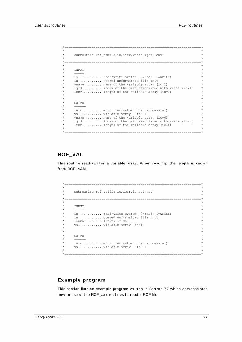
User subroutines ROF routines
DarcyTools 2.1 31
*======================================================================* * * * subroutine rof_nam(io,iu,ierr,vname,igrd,lenv) * * * *======================================================================* * * * INPUT * * ----- * * io ........... read/write switch (0=read, 1=write) * * iu ........... opened unformatted file unit * * vname ........ name of the variable array (io=1) * * igrd ......... index of the grid associated with vname (io=1) * * lenv ......... length of the variable array (io=1) * * * * * * OUTPUT * * ------ * * ierr ......... error indicator (0 if successful) * * val .......... variable array (io=0) * * vname ........ name of the variable array (io=0) * * igrd ......... index of the grid associated with vname (io=0) * * lenv ......... length of the variable array (io=0) * * * *======================================================================*
ROF_VAL
This routine reads/writes a variable array. When reading: the length is known
from ROF_NAM.
*======================================================================* * * * subroutine rof_val(io,iu,ierr,lenval,val) * * * *======================================================================* * * * INPUT * * ----- * * io ........... read/write switch (0=read, 1=write) * * iu ........... opened unformatted file unit * * lenval ....... length of val * * val .......... variable array (io=1) * * * * * * OUTPUT * * ------ * * ierr ......... error indicator (0 if successful) * * val .......... variable array (io=0) * * * *======================================================================*
Example program
This section lists an example program written in Fortran 77 which demonstrates
how to use of the ROF_xxx routines to read a ROF file.
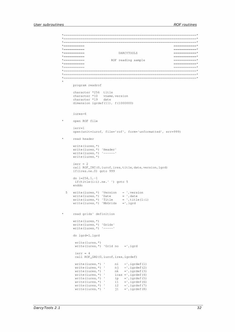
User subroutines ROF routines
DarcyTools 2.1 32
*======================================================================* *======================================================================* *======================================================================* *=========== ============* *=========== ============* *=========== DARCYTOOLS ============* *=========== ============* *=========== ROF reading sample ============* *=========== ============* *=========== ============* *======================================================================* *======================================================================* *======================================================================* * program readrof character *256 title character *10 vname,version character *19 date dimension igrdef(11), f(1000000) iures=6 * open ROF file ierr=1 open(unit=iurof, file='rof', form='unformatted', err=999) * read header write(iures,*) write(iures,*) 'Header' write(iures,*) '------' write(iures,*) ierr = 2 call ROF_INI(0,iurof,ires,title,date,version,lgrd) if(ires.ne.0) goto 999 do i=256,1,-1 if(title(i:i).ne.' ') goto 5 enddo 5 write(iures,*) 'Version = ',version write(iures,*) 'Date = ',date write(iures,*) 'Title = ',title(1:i) write(iures,*) 'NbGrids =',lgrd * read grids' definition write(iures,*) write(iures,*) 'Grids' write(iures,*) '-----' do igrd=1,lgrd write(iures,*) write(iures,*) 'Grid no =',igrd ierr = 4 call ROF_GRD(0,iurof,ires,igrdef) write(iures,*) ' ni =',igrdef(1) write(iures,*) ' nj =',igrdef(2) write(iures,*) ' nk =',igrdef(3) write(iures,*) ' icas =',igrdef(4) write(iures,*) ' ip =',igrdef(5) write(iures,*) ' i1 =',igrdef(6) write(iures,*) ' i2 =',igrdef(7) write(iures,*) ' j1 =',igrdef(8)
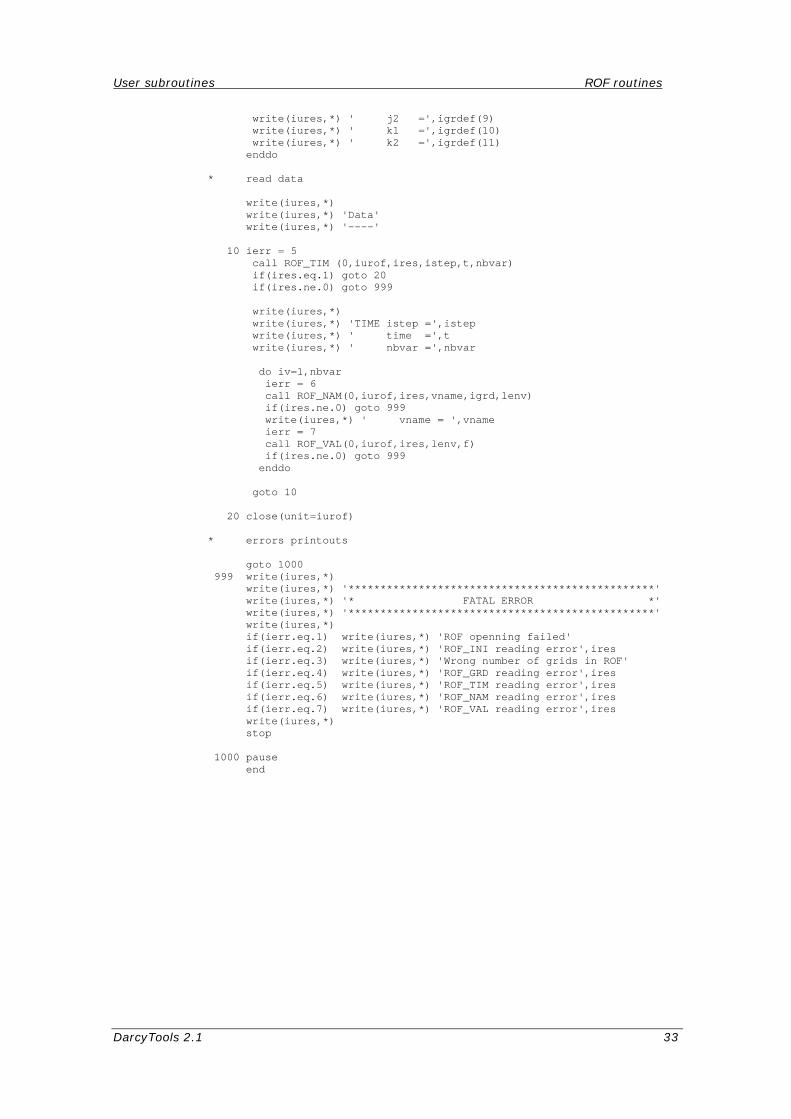
User subroutines ROF routines
DarcyTools 2.1 33
write(iures,*) ' j2 =',igrdef(9) write(iures,*) ' k1 =',igrdef(10) write(iures,*) ' k2 =',igrdef(11) enddo * read data write(iures,*) write(iures,*) 'Data' write(iures,*) '----' 10 ierr = 5 call ROF_TIM (0,iurof,ires,istep,t,nbvar) if(ires.eq.1) goto 20 if(ires.ne.0) goto 999 write(iures,*) write(iures,*) 'TIME istep =',istep write(iures,*) ' time =',t write(iures,*) ' nbvar =',nbvar do iv=1,nbvar ierr = 6 call ROF_NAM(0,iurof,ires,vname,igrd,lenv) if(ires.ne.0) goto 999 write(iures,*) ' vname = ',vname ierr = 7 call ROF_VAL(0,iurof,ires,lenv,f) if(ires.ne.0) goto 999 enddo goto 10 20 close(unit=iurof) * errors printouts goto 1000 999 write(iures,*) write(iures,*) '************************************************' write(iures,*) '* FATAL ERROR *' write(iures,*) '************************************************' write(iures,*) if(ierr.eq.1) write(iures,*) 'ROF openning failed' if(ierr.eq.2) write(iures,*) 'ROF_INI reading error',ires if(ierr.eq.3) write(iures,*) 'Wrong number of grids in ROF' if(ierr.eq.4) write(iures,*) 'ROF_GRD reading error',ires if(ierr.eq.5) write(iures,*) 'ROF_TIM reading error',ires if(ierr.eq.6) write(iures,*) 'ROF_NAM reading error',ires if(ierr.eq.7) write(iures,*) 'ROF_VAL reading error',ires write(iures,*) stop 1000 pause end

Appendix B Structure of SOLVE
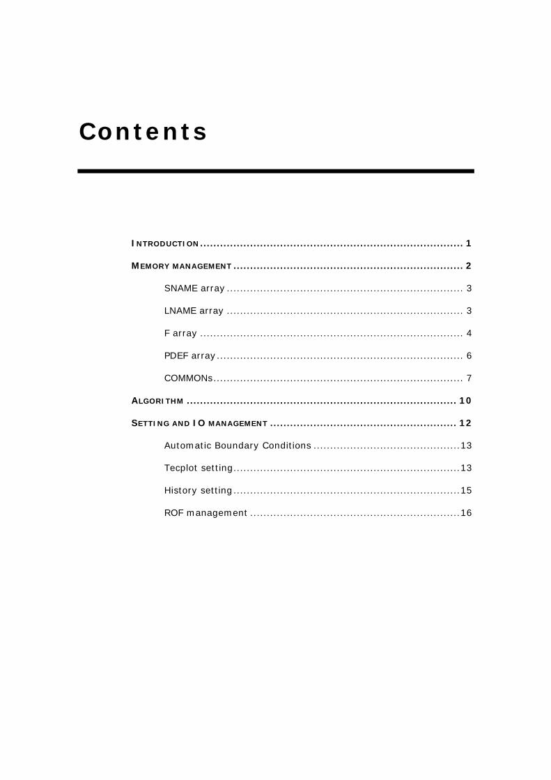
Contents
INTRODUCTION............................................................................... 1
MEMORY MANAGEMENT ..................................................................... 2
SNAME array ....................................................................... 3
LNAME array ....................................................................... 3
F array ............................................................................... 4
PDEF array.......................................................................... 6
COMMONs........................................................................... 7
ALGORITHM ................................................................................. 10
SETTING AND IO MANAGEMENT ........................................................ 12
Automatic Boundary Conditions ............................................13
Tecplot setting....................................................................13
History setting....................................................................15
ROF management ...............................................................16
Structure of SOLVE Introduction
DarcyTools 2.1 1
Structure of SOLVE
Introduction
When associated to the MIGAL library, the code is split in several sections and
forms three accessibility levels. A top User level is made of template user’s
routines, a mid Developer level is made of the Main, Setting, Geometric, IO,
Utilities, Physics, Models and Numerical Sections and a low “Not-Accessible”
Level is made of MIGAL’s subroutines. The different sections encapsulate the
routines in the following way:
NUM-Section: The numerical discretisation procedures SETOPx where x is 1
for BFC, 2 for BFC:S and 3 for Cartesian grids.
SET-Section: The memory and setting management.
GEOM-Section: The mesh generation facilities, metric calculations and the
read/write format for grid files.
IO-Section: The ROF and TEC input-output procedures.
PHYS-Section: The physical fluid and rock laws encoding.
MOD-Section: The special procedures for boundary and source/sink conditions
or properties like GWRT, FRAME or TUNNEL and the PARTRACK
routines.
UTIL-Section: The utility routines for safe programming.
USER-Section: Templates routines for user control.
The User-Section is a set of template routines automatically called by the
program that the users can complete to define and control the calculations.
Among those routines, whose names follow the pattern URSxxxxx, the USRSET
routine is dedicated to case definition. To program the user’s routine, a set of
routines, whose names follow the pattern SETxxxxx is provided in the Set-
Section.

Structure of SOLVE Memory management
DarcyTools 2.1 2
Figure 1 : Code structure and main dependencies
The Numerical, Geometrical and IO sections of the DarcyTools solver have been
written in FORTAN 77 for sake of portability and maintenance. Only part of the
upper level, concerned by memory management and user interface, is written in
FORTRAN 90. In that case, mainly the pointers allocation capability feature is
used.
Memory management
To enable various scenarios to run without compilation and manual adjustments
DarcyTools uses a self adaptive memory management written in FORTRAN 90
and entirely located into the Setting Section of the program. This memory
management is based on a single F array allocation technique for the numerical
part of the program and on several annex arrays dedicated to the storage of the
setting.
Num-Section
User Level
Developer Level
Protected Level
Set-Section
Main-Section
Geom-Section
IO-Section
User-Section
Util-Section
Mod-Section
Phys-Section
MIGAL
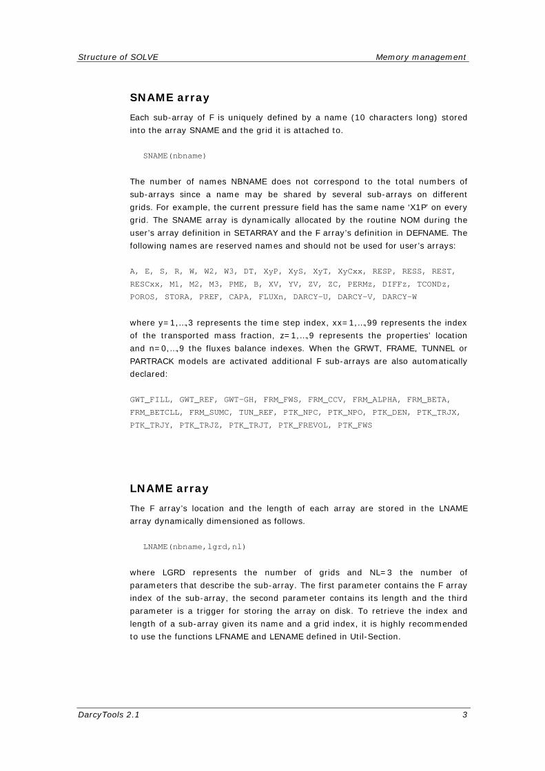
Structure of SOLVE Memory management
DarcyTools 2.1 3
SNAME array
Each sub-array of F is uniquely defined by a name (10 characters long) stored
into the array SNAME and the grid it is attached to.
SNAME(nbname)
The number of names NBNAME does not correspond to the total numbers of
sub-arrays since a name may be shared by several sub-arrays on different
grids. For example, the current pressure field has the same name ‘X1P’ on every
grid. The SNAME array is dynamically allocated by the routine NOM during the
user’s array definition in SETARRAY and the F array’s definition in DEFNAME. The
following names are reserved names and should not be used for user’s arrays:
A, E, S, R, W, W2, W3, DT, XyP, XyS, XyT, XyCxx, RESP, RESS, REST, RESCxx, M1, M2, M3, PME, B, XV, YV, ZV, ZC, PERMz, DIFFz, TCONDz, POROS, STORA, PREF, CAPA, FLUXn, DARCY-U, DARCY-V, DARCY-W
where y=1,…,3 represents the time step index, xx=1,…,99 represents the index
of the transported mass fraction, z=1,…,9 represents the properties’ location
and n=0,…,9 the fluxes balance indexes. When the GRWT, FRAME, TUNNEL or
PARTRACK models are activated additional F sub-arrays are also automatically
declared:
GWT_FILL, GWT_REF, GWT-GH, FRM_FWS, FRM_CCV, FRM_ALPHA, FRM_BETA, FRM_BETCLL, FRM_SUMC, TUN_REF, PTK_NPC, PTK_NPO, PTK_DEN, PTK_TRJX, PTK_TRJY, PTK_TRJZ, PTK_TRJT, PTK_FREVOL, PTK_FWS
LNAME array
The F array’s location and the length of each array are stored in the LNAME
array dynamically dimensioned as follows.
LNAME(nbname,lgrd,nl)
where LGRD represents the number of grids and NL=3 the number of
parameters that describe the sub-array. The first parameter contains the F array
index of the sub-array, the second parameter contains its length and the third
parameter is a trigger for storing the array on disk. To retrieve the index and
length of a sub-array given its name and a grid index, it is highly recommended
to use the functions LFNAME and LENAME defined in Util-Section.
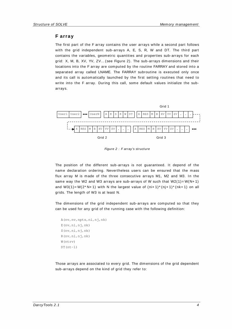
Structure of SOLVE Memory management
DarcyTools 2.1 4
F array
The first part of the F array contains the user arrays while a second part follows
with the grid independent sub-arrays A, E, S, R, W and DT. The third part
contains the variables, geometric quantities and properties sub-arrays for each
grid: X, M, B, XV, YV, ZV… (see Figure 2). The sub-arrays dimensions and their
locations into the F array are computed by the routine FARRAY and stored into a
separated array called LNAME. The FARRAY subroutine is executed only once
and its call is automatically launched by the first setting routines that need to
write into the F array. During this call, some default values initialize the sub-
arrays.
Figure 2 : F array’s structure
The position of the different sub-arrays is not guaranteed. It depend of the
name declaration ordering. Nevertheless users can be ensured that the mass
flux array M is made of the three consecutive arrays M1, M2 and M3. In the
same way the W2 and W3 arrays are sub-arrays of W such that W2(1)=W(N+1)
and W3(1)=W(2*N+1) with N the largest value of (ni+1)*(nj+1)*(nk+1) on all
grids. The length of W3 is at least N.
The dimensions of the grid independent sub-arrays are computed so that they
can be used for any grid of the running case with the following definition:
A(nv,nv,npts,ni,nj,nk) E(nv,ni,nj,nk) S(nv,ni,nj,nk) R(nv,ni,nj,nk) W(ntrv)
DT(nt-1)
Those arrays are associated to every grid. The dimensions of the grid dependent
sub-arrays depend on the kind of grid they refer to:
DT A S R E
…Grid 2 Grid 3
User2 User1 … UserN
Grid 1
W
X M B XV ZV YV . . . RES X M B XV ZV YV . . . RES
X M B XV ZV YV . . . RES

Structure of SOLVE Memory management
DarcyTools 2.1 5
BFC BFC:s CART
X(ni,nj,nk,nx,nt) X(ni,nj,nk,nx,nt) X(ni,nj,nk,nx,nt) RES(nx) RES(nx) RES(nx) M(ni,nj,nk,3) M(ni,nj,nk,3) M(ni,nj,nk,3) B(31,ni,nj,nk) - - XV(ni+1,nj+1,nk+1) XV(ni+1) XV(ni+1) YV(ni+1,nj+1,nk+1) YV(nj+1) YV(nj+1) ZV(ni+1,nj+1,nk+1) ZV(ni+1,nj+1,nk+1) ZV(nk+1) - ZC(ni,nj,nk) -
The parameters nv, nt and nx are grid independent and represent respectively
the number of coupled variables (1 for the segregated approach, 2 for the
coupled pressure-salinity approach), the number of time steps involved in the
time discretisation and the number of variables contained in the X array (e.g 2
for a pressure-salinity problem).
The parameters npts, ni, nj and nk are grid dependent and represent
respectively the width of the discretisation stencil (i.e. 7 for 3D, 5 for 2D and 3
for 1D), and the number of cells in x, y and z direction.
For memory storage saving, users can define uniform properties as being single
element long sub-arrays via routine SETF0. The concerned sub-arrays are:
PERMz, DIFFz, TCONDz, POROS, STORA, PREF, CAPA
Finally, for top boundary condition facility a two dimensional sub-array is defined
on the very parent grid only PME(ni,nj).
sub-arrays
DT the values of the present (1) and the previous (2…) time steps for
time derivative evaluation when nt>0.
RES the Log10 of the mean square residual of the variables. The names
for accessing that array are RESP, RESS and RESxx accordingly to the
variable order.
A the operator coefficients ordered for MIGAL.
E a work array used to contain the estimation of the solution during
MIGAL computation.
S the operator source term for MIGAL.
R a work array that contains the residual field returned by MIGAL. It
also temporarily contains the cell centre z-coordinates in BFC:s case.
W a work array for MIGAL. It also temporarily contains the Qsrc and Qphi
arrays used for user’s definition of boundary and sources/sinks terms.
X the variables fields from 1 to nx for the present time (1) and the
previous time steps (2…nt). The pressure index is fixed at 1 and the
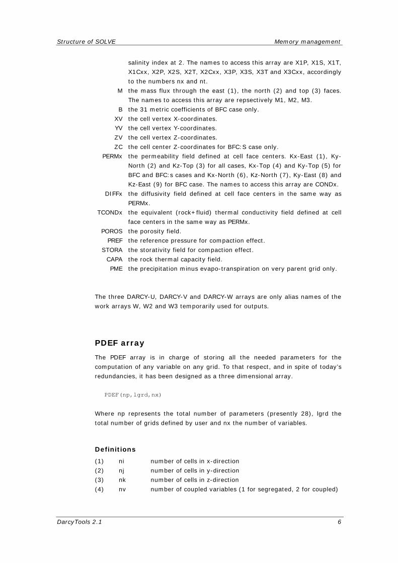
Structure of SOLVE Memory management
DarcyTools 2.1 6
salinity index at 2. The names to access this array are X1P, X1S, X1T,
X1Cxx, X2P, X2S, X2T, X2Cxx, X3P, X3S, X3T and X3Cxx, accordingly
to the numbers nx and nt.
M the mass flux through the east (1), the north (2) and top (3) faces.
The names to access this array are repsectively M1, M2, M3.
B the 31 metric coefficients of BFC case only.
XV the cell vertex X-coordinates.
YV the cell vertex Y-coordinates.
ZV the cell vertex Z-coordinates.
ZC the cell center Z-coordinates for BFC:S case only.
PERMx the permeability field defined at cell face centers. Kx-East (1), Ky-
North (2) and Kz-Top (3) for all cases, Kx-Top (4) and Ky-Top (5) for
BFC and BFC:s cases and Kx-North (6), Kz-North (7), Ky-East (8) and
Kz-East (9) for BFC case. The names to access this array are CONDx.
DIFFx the diffusivity field defined at cell face centers in the same way as
PERMx.
TCONDx the equivalent (rock+fluid) thermal conductivity field defined at cell
face centers in the same way as PERMx.
POROS the porosity field.
PREF the reference pressure for compaction effect.
STORA the storativity field for compaction effect.
CAPA the rock thermal capacity field.
PME the precipitation minus evapo-transpiration on very parent grid only.
The three DARCY-U, DARCY-V and DARCY-W arrays are only alias names of the
work arrays W, W2 and W3 temporarily used for outputs.
PDEF array
The PDEF array is in charge of storing all the needed parameters for the
computation of any variable on any grid. To that respect, and in spite of today’s
redundancies, it has been designed as a three dimensional array.
PDEF(np,lgrd,nx)
Where np represents the total number of parameters (presently 28), lgrd the
total number of grids defined by user and nx the number of variables.
Definitions
(1) ni number of cells in x-direction
(2) nj number of cells in y-direction
(3) nk number of cells in z-direction
(4) nv number of coupled variables (1 for segregated, 2 for coupled)

Structure of SOLVE Memory management
DarcyTools 2.1 7
(5) npts width of stencil (7 for 3D, 5 for 2D, 3 for 1D).
(6) - undefined
(7) iunit opened logical unit for MIGAL’s printings
(8) icycle kind of MIGAL’s multi-grid cycle
(9) nbgrid depth of MIGAL’s multi-grid cycles
(10) liter maximum number of cycles for MIGAL
(11) nbrelax number of relaxations on each MIGAL’s multi-grid level
(12) iform kind of operator organization for MIGAL (always 0)
(13) igmres depth of GMRES sub-space
(14) ipreco number of GMRES preconditioning iteration
(15) resfac desired residual reduction before leaving MIGAL
(16) relax ILU0 relaxation factor for MIGAL
(17) relin relaxation factor applied to the MIGAL solution
(18) ntv number of time steps involved in time discretisation
(19) nx number of variables in X array
(20) icas kind of grid (1 for BFC, 2 for BFC:s, 3 for CART)
(21) ip index of the parent grid
(22) i1 first parent cell index of the grid footprint in x-direction
(23) i2 last parent cell index of the grid footprint in x-direction
(24) j1 first parent cell index of the grid footprint in y-direction
(25) j2 last parent cell index of the grid footprint in y-direction
(26) k1 first parent cell index of the grid footprint in z-direction
(27) k2 last parent cell index of the grid footprint in z-direction
(28) iflu embedded boundary conditions (1 fixed fluxes, 2 fixed values)
(29) nbprer number of pre-restriction relaxations for MIGAL
(30) igms depth of GMRES sub-space smoother for MIGAL
COMMONs
To simplify the user’s routines programming some parameters and variables are
stored into commons. In principle, users are not allowed to change any values in
the following commons:
common /memor1/ f, pdef common /memor2/ lname,sname common /memor3/ bossdef, nboss common /memor4/ ftec,ztec,btec,stec,nftec,nztec,nbtec common /memor5/ tihist,vnhist,lphist,nbhist,nbvhist,nbphist common /memor6/ flubdef(7,10) common /memor7/ indgrd,lindg common /memor8/ fxdiff,vrm,vim,pfp,cumfac,alpha,volrp, & pip,typep,adtypp,adstap common /iufile/ iures,iurof,iuhist common /server/ idport common /const0/ dtini,t1,t2,nt1,nt2

Structure of SOLVE Memory management
DarcyTools 2.1 8
common /const1/ g common /const2/ nstep,nsweep,nvar1,nvar2,nitc1, & nvar3,nvar4, nitc2,nvar5,nvar6,nitg common /const3/ istep,isweep,igrd,itc,ivar,itg,t common /const4/ np,lgrd,nbname,nl,lf common /const5/ title, version, date common /const6/ hx,hy,hz common /const7/ precdif common /const8/ istep1,istep2,istepfr,irst common /const9/ grdfile common /defv1 / poros,stora,pref,capa,tcond(9),perm(9),diff(9) common /defv2 / iporos,istora,ipref,icapa,itcond(9), & iperm(9),idiff(9) common /law1 / rho0, trho, alpha1, alpha2, beta1, beta2 common /law2 / amu0, amu1, amu2, tmu, n_mu common /law3 / acp0, acp1, acp2 common /tun/ itundef,tunsec,ntun_p,ntun_c,ntun_s,nsec_p common /frm / nalint,alphl,alphh,frmk,bettot common /gwt / grlx,facmin common /ptk01 / npd,nptk,method,igptk,ptkfile,nleave,narriv common /ptk02 / is1,is2,js1,js2,ks1,ks2 common /ptk03 / ie1,ie2,je1,je2,ke1,ke2 common /ptk04 / nalint,alphl,alphh,ak,bettot,fxdiff,retmob & nmobst,naintn common /ptk05 / pfsta(3),tsteph,wnstph(3) common /ptk06 / seed common /ptk07 / nbtrj,ntrjfr,lentrj,ltrj common /ptk08 / nolond,adsorp common /bndy1 / ssea,tsea,tland common /bands / lbndp,lbndn,lbnds,lbnde,lbndw,lbndt,lbndb common /solve2/ licence, path, lenpath
Beside these and for simplicity, a common is also dedicated to the exchange of
MIGAL’s control parameters between the program and the user’s routine
USRSLV.
common /solve1/ icycle, nbgrid, liter, nbrelax, igmres, ipreco & iusolv, resfac, relax, relin
Definitions
/memor1/ contains the F and PDEF pointers
/memor2/ contains the sub-arrays locations and names
/memor3/ contains the setting for automatic boundary conditions

Structure of SOLVE Memory management
DarcyTools 2.1 9
/memor4/ contains the setting for Tecplot outputs
/memor5/ contains the setting for history visualization
/memor6/ contains the setting for mass fluxes balances outputs
/memor7/ contains the INDGRD pointers
/memor8/ contains pointers on the internal PARTRACK work arrays
/iufile/ contains the logical unit for RESULT, ROF and HISTxx files
/server/ contains the monitoring server port ID
/const0/ contains the time step zoning parameters
/const1/ contains the gravity constant
/const2/ contains the loops definition of the algorithm
/const3/ contains the current index of the loops and the current time value
/const4/ contains some arrays dimensions
/const5/ contains the run definition strings
/const6/ contains the default grid dimensions
/const7/ contains the preconditioning parameter
/const8/ contains the ROF outputs definition and the RESTART trigger.
/const9/ contains the grid file name for reading the initial grid.
/defv1/ contains the initial value of properties.
/defv2/ contains properties parameters for SET_xx and GET_xx optimization
/law1/ contains the density state law parameters
/law2/ contains the viscosity state law parameters
/law3/ contains the specific heat state law parameters
/tun/ contains the setting for the TUNNEL model
/frm/ contains the setting for the FRAME model
/gwt/ contains the setting for the GRWT model
/ptk01/ contains the setting for the PARTRACK model
/ptk02/ contains the definition of the PARTRACK emission box
/ptk03/ contains the definition of the PARTRACK capturing box
/ptk04/ contains the setting for the PARTRACK multi-rate model
/ptk05/ contains the setting for the PARTRACK method 1
/ptk06/ contains the seed for PARTRACK random kernel
/ptk07/ contains the setting for PARTRACK trajectories
/ptk08/ contains the PARTRACK diffusion-adsorption triggers
/bndy1/ contains the setting for the top boundary conditions
/bands/ contains the band indexes for operator A array
/solve1/ contains MIGAL’s parameters temporarily overwritten by user
/solve2/ contains the MIGAL unlocking information
Naturally, users can create other commons to exchange data between several
user’s routines, for example between the setting case routine URSSET and the
boundary conditions routines USRBOSS.
Users should also note that all the reserved logical units are not present in the
common /iufile/. Hence, it is highly recommended to use the routine IUFREE of
Util-Section to get a free unit number when needed.

Structure of SOLVE Algorithm
DarcyTools 2.1 10
Algorithm
The DarcyTools algorithm is encapsulated into the Main Section of the program.
It consists of several nested loops sequentially solving variables and/or groups
of variables. The external loop is the time integration loop running from 1 to
nstep. The second loop is the grid sequence loop running from the most
embedded grid level lgrd to the largest grid level 1. For each time step and each
grid, the computation of the nx variables is split in three groups defined by the
nvar1 to nvar6 parameters.
Figure 3 : Main algorithm and loops nomenclature
MAIN
DO ivar = nvar3, nvar4
DO itg = 1, nitg
DO ivar = nvar1, nvar2
DO igrd = lgrd, 1, -1
DO isweep = 1, nsweep
Solve variable ivar
ENDDO
ENDDO
DO itc = 1, nitc1
Solve variable ivar
ENDDO
ENDDO
DO ivar = nvar5, nvar6
Solve variable ivar
ENDDO
ENDDO
ENDDO
DO itc = 1, nitc2
ENDDO
Setting & Initializations
DO istep = 1, nstep
ENDDO
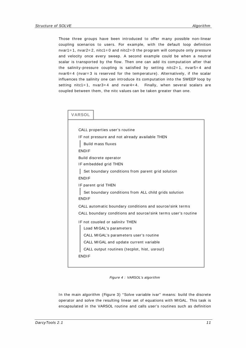
Structure of SOLVE Algorithm
DarcyTools 2.1 11
Those three groups have been introduced to offer many possible non-linear
coupling scenarios to users. For example, with the default loop definition
nvar1=1, nvar2=2, nitc1=0 and nitc2=0 the program will compute only pressure
and velocity once every sweep. A second example could be when a neutral
scalar is transported by the flow. Then one can add its computation after that
the salinity-pressure coupling is satisfied by setting nitc2=1, nvar5=4 and
nvar6=4 (nvar=3 is reserved for the temperature). Alternatively, if the scalar
influences the salinity one can introduce its computation into the SWEEP loop by
setting nitc1=1, nvar3=4 and nvar4=4. Finally, when several scalars are
coupled between them, the nitc values can be taken greater than one.
Figure 4 : VARSOL’s algorithm
In the main algorithm (Figure 3) “Solve variable ivar” means: build the discrete
operator and solve the resulting linear set of equations with MIGAL. This task is
encapsulated in the VARSOL routine and calls user’s routines such as definition
CALL boundary conditions and source/sink terms user’s routine
IF not pressure and not already available THEN
IF not coupled or salinity THEN
CALL properties user’s routine
Build discrete operator
ENDIF
Build mass fluxes
Set boundary conditions from parent grid solution ENDIF
Set boundary conditions from ALL child grids solution ENDIF
Load MIGAL’s parameters
ENDIF
CALL MIGAL’s parameters user’s routine CALL MIGAL and update current variable CALL output routines (tecplot, hist, usrout)
IF parent grid THEN
IF embedded grid THEN
VARSOL
CALL automatic boundary conditions and source/sink terms
Structure of SOLVE Setting and IO management
DarcyTools 2.1 12
of properties, boundary conditions and source/sink terms, overwriting of the
MIGAL parameters and printings.
The ITG loop ensures the convergence of the mutual influence of the grid levels
of cases running with embedded grids.
The mass fluxes are usually computed during the construction of the operator
for pressure or after a pressure update. Nevertheless, if the pressure is a fixed
input and one only uses DarcyTools for scalar transport, the mass fluxes are
automatically built.
When the coupled pressure-salinity solution is selected, the VARSOL routine
does not call MIGAL for the pressure but wait until the salinity is called to solve
them together. Hence, there is a restriction in the ivar loops definition: when
coupled, the pressure (ivar=1) must always immediately precede the salinity
(ivar=2).
The routines PROPS and BOSS are respectively in charge of calling the model
routines (TUNNEL, GRWT, FRAME…) of setting the default and automatic
conditions stipulated by users and of calling the routines USRPROP and
USRBOSS.
Before calling MIGAL, an opportunity is given to users of adapting the solver
parameters depending on the current solution, grid, or iteration via the routine
USRSLV. For coupled iterations, the opportunity to modify the preconditioned
operator is also given via the routine USRPRECO.
Finally, after every MIGAL’s run, the template routine USROUT is called for
user’s outputs. By checking the iteration variables in common /const3/ the user
is informed of the very moment of this call. This routine is also called once per
grid after initialization, just before starting the time integration loop. Then ivar is
null and igrd represents the grid index (i.e. 1 for the largest grid, lgrd for the
most embedded grid).
Setting and IO management
Beside the numerical calculations DarcyTools implements a user interface for
setting and Input/Output purpose. Those additional features have been
separated from the F array memory management for the sake of clarity. Three
commons have been designed for this task, namely /memor3/, /memor4/ and
/memor5/.

Structure of SOLVE Setting and IO management
DarcyTools 2.1 13
Automatic Boundary Conditions
The common /memor3/ is in charge of storing the automatic source/sink
boundary conditions setting. It contains a two dimensional array BOSSDEF and
the number NBOSS of automatic conditions stipulated by the user.
BOSSDEF(13,nboss)
BOSSDEF
This array is dynamically allocated by the routine SETBOSS and, for each
boundary condition, stores the following information:
(1) ivar X array’s index of the variable
(2) igrd index of the grid
(3) i1 lower bound of the footprint in x direction
(4) i2 upper bound of the footprint in x direction
(5) j1 lower bound of the footprint in y direction
(6) j2 upper bound of the footprint in y direction
(7) k1 lower bound of the footprint in z direction
(8) k2 upper bound of the footprint in z direction
(9) it1 lower bound of the footprint in time
(10) it2 upper bound of the footprint in time
(11) qsrc explicit part of the source term to apply to the footprint
(12) qphi implicit part of the source term to apply to the footprint
(13) itype type of source term condition (0 uniform, 1 fixed in time)
Given the array BOSSDEF, the routine BOSS will automatically apply the
specified source/sink boundary condition to the specified footprint before calling
the USRBOSS routine but after DEFBC which fixes the default top boundary
conditions and the PME masse sources. This feature allows for example to repeat
or change the boundary conditions from the initial ones during time integration.
Tecplot setting
The common /memor4/ is in charge of storing the user’s commands relative to
the Tecplot output facilities. It contains four two dimensional arrays FTEC, ZTEC,
BTEC and STEC as well as the number NFTEC of files to create, the total number
NZTEC of zone’s definitions and the number NBTEC of block’s definitions.

Structure of SOLVE Setting and IO management
DarcyTools 2.1 14
FTEC(4, nftec) ZTEC(16,nztec) BTEC(4, nbtec) STEC(2, nbtec)
FTEC
The FTEC array is dynamically allocated by the routine SETTECF and stores the
following information about the file created by DarcyTools to write the desired
Tecplot data set.
(1) iunit locical unit number of the opened file
(2) is_grid kind of mesh (0=no mesh, 1=cell centers, 2=cell vertexes)
(3) lastzone last zone written in the file for duplicating information
(4) isbinary unused
ZTEC
The ZTEC array is dynamically allocated by the routine SETTECZ and stores the
information relative to the zones extents.
(1) nbcall counter for zone naming
(2) i1 lower bound of the outputs in x direction
(3) i2 upper bound of the outputs in x direction
(4) ifr increment value of outputs in x direction
(5) j1 lower bound of the outputs in y direction
(6) j2 upper bound of the outputs in y direction
(7) jfr increment value of the outputs in x direction
(8) k1 lower bound of the outputs in z direction
(9) k2 upper bound of the outputs in z direction
(10) kfr increment value of outputs in z direction
(11) it1 lower bound of the outputs in time
(12) it2 upper bound of the outputs in time
(13) itfr increment value of outputs in time
(14) ifile index of the concerned file (in FTEC)
(15) igrid index of the associated grid
(16) ivar trigger variable index for writing activation
BTEC
The BTEC array is dynamically allocated by the routine SETTECB and stores the
F sub-arrays name index of the values to write in the data set.
Structure of SOLVE Setting and IO management
DarcyTools 2.1 15
(1) iaction type of action to perform on the data before output
(2) value value for the action iaction
(3) ifile index of the concerned grid (in FTEC)
(4) ivname index of the sub-array name (in SNAME)
STEC
The STEC array is dynamically allocated by the routine SETTECF and stores the
output file name and the title of the data set into 256 characters long strings.
(1) filename file name for output (including path)
(2) title index of the sub-array name (in SNAME)
Given all this information, DarcyTools automatically call the relevant routines
TECxxx of the IO_section via the routine TECPLOT in order to create outputs
data files directly readable by the post-processing software Tecplot.
History setting
The common /memor5/ is in charge of storing the user’s commands relative to
the history visualization facilities. It contains three arrays TIHIST, VNHIST and
LPHIST, as well as the number NBHIST of files (graph) to create, the maximum
number NBVHIST of plots allowed per graph and the number NBPHIST of
parameters of the graph definition.
TIHIST(nbhist) VNHIST(nbhist,nbvhist) LPHIST(nbhist,nbphist)
TIHIST
The TIHIST array is in charge of storing the 35 characters long strings dedicated
to the title of the graphs.
VNHIST
The VNHIST array is in charge of storing the 10 characters long strings that
contain the label of every variable of the graph.
Structure of SOLVE Setting and IO management
DarcyTools 2.1 16
LPHIST
The LPHIST array is in charge of storing the curves definition of the graphs with
the following convention:
(1-nbvhist) sub-array indexes of the values to plot in plotting order.
(nbvhist +1) I position index
(nbvhist +2) J position index
(nbvhist +3) K position index
(nbvhist +4) index of the concerned grid
(nbvhist +5) X index of the variable triggering the outputs
(nbvhist +6) writing counter for abscise coordinate
Given all this information, DarcyTools automatically creates a HIST.HTM file and
several HISTxx files via the routine HIST for real time history visualization via a
web browser.
A HIST00 file is also automatically created which contains an ON/OFF trigger and
the STEP and SWEEP current values. The ON/OFF trigger is periodically read by
DarcyTools in order to know if it should stop or go on computing the next time
step integration. Hence a visualization program can stop DarcyTools before its
last time step by removing the file HIST00 or by setting the ON/OFF trigger (first
line) to 0. Then DarcyTools terminates the current time step and saves all the
required information like it would have done during the last time step.
ROF management
DarcyTools also implements in the subroutine ROF an automatic restart and an
intermediary result storage facility.
In any case, DarcyTools creates an unformatted ROF file to store on disk, after
the last time step, the minimum information to proceed to restart. If necessary,
users may also use this ROF file to automatically store intermediary results for
certain time steps. In that case, DarcyTools raises to 1 the third parameter in
the LNAME array for the user selected sub-arrays, and stores the first, the last
and the increment time steps indexes into the common /const8/.
When a restart is ordered DarcyTools raises to 1 the variable IRST of the
common /const8/ and starts by reading the file ROF.
The IO low level ROF_xxx routines as well as the TEC_xxx routines have been
gathered into an IO-Section to provide users with a library for post processing
data. All those low level IO routines are written in Fortran 77.

Appendix C Four CIF-examples

********************************************************** * * * Test of grids, (Case A4) * * * * 26 December 2003 * * * ********************************************************** * 1 SETTITLE : title 1 'Test of Grids' * 2 SETGRDF : fname 2 'xyz' * 3 SETLICM : licence, path 3 'aa8vMYhrHd8VqPMWq3Lm' '' * 6 SETSTEP : dt nstep iorder 6 0.31636E-2 100 1 * 12 SETLAW1 : rho0, Trho, alpha1, alpha2, beta1, beta2 12 1000. 0. 0.008 0. 0. 0. * 13 SETLAW2 : visc0, a1, a2, Tvisc, n 13 2.E-3 0. 0. 0. 1 * 110 SETSWEEP : nsweep, ivar1, ivar2 110 1 1 2 * 118 SETF1 : name, igrd, value 118 'PERM1' 1 2.E-4 118 'PERM2' 1 2.E-4 118 'PERM3' 1 2.E-4 * 118 'PERM4' 1 2.E-4 * 118 'PERM5' 1 2.E-4 * 118 'PERM6' 1 2.E-4 * 118 'PERM7' 1 2.E-4 * 118 'PERM8' 1 2.E-4 * 118 'PERM9' 1 2.E-4 118 'DIFF1' 1 1. 118 'DIFF2' 1 1. 118 'DIFF3' 1 1. * 118 'DIFF4' 1 1. * 118 'DIFF5' 1 1. * 118 'DIFF6' 1 1. * 118 'DIFF7' 1 1. * 118 'DIFF8' 1 1. * 118 'DIFF9' 1 1. 118 'POROS' 1 1.E-3 * 121 SETSPT : s1, t1, s0, t0, dwt, dsdz, dtdz, i1, i2 j1, j2, k1, k2 121 0. 0. 1. 0. 0. -2.0E-3 0. 1 50 1 50 1 50 * 122 SETBOSS : ivar, igrd, itype, i1, i2, j1, j2, k1, k2, it1, it2, qsrc, qphi 122 1 1 1 1 1 1 50 1 50 1 950 0. 0. 122 1 1 1 50 50 1 50 1 50 1 950 0. 0. 122 1 1 1 1 50 1 1 1 50 1 950 0. 0. 122 1 1 1 1 50 50 50 1 50 1 950 0. 0. 122 1 1 1 1 50 1 50 1 1 1 950 0. 0. 122 1 1 1 1 50 1 50 50 50 1 950 0. 0.
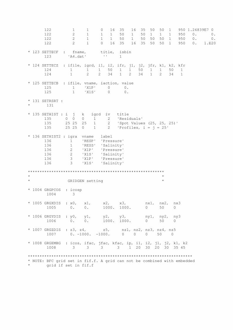
122 1 1 0 16 35 16 35 50 50 1 950 1.26839E7 0 122 2 1 1 1 50 1 50 1 1 1 950 0. 0. 122 2 1 1 1 50 1 50 50 50 1 950 0. 0. 122 2 1 0 16 35 16 35 50 50 1 950 0. 1.E20 * 123 SETTECF : fname, title, isbin 123 'A4.dat' '' 1 * 124 SETTECZ : ifile, igrd, i1, i2, ifr, j1, j2, jfr, k1, k2, kfr 124 1 1 1 50 1 1 50 1 1 50 1 124 1 2 2 34 1 2 34 1 2 34 1 * 125 SETTECB : ifile, vname, iaction, value 125 1 'X1P' 0 0. 125 1 'X1S' 0 0. * 131 SETRSRT : * 131 * 135 SETHIST : i j k igrd iv title 135 0 0 0 1 2 'Residuals' 135 25 25 25 1 2 'Spot Values (25, 25, 25)' 135 25 25 0 1 2 'Profiles, i = j = 25' * 136 SETHIST2 : igra vname label 136 1 'RESP' 'Pressure' 136 1 'RESS' 'Salinity' 136 2 'X1P' 'Pressure' 136 2 'X1S' 'Salinity' 136 3 'X1P' 'Pressure' 136 3 'X1S' 'Salinity' ********************************************************** * * * GRIDGEN setting * * 1004 GRGPCOS : icosp 1004 3 * 1005 GRGXDIS : x0, x1, x2, x3, nx1, nx2, nx3 1005 0. 0. 1000. 1000. 0 50 0 * 1006 GRGYDIS : y0, y1, y2, y3, ny1, ny2, ny3 1006 0. 0. 1000. 1000. 0 50 0 * 1007 GRGZDIS : z3, z4, z5, nz1, nz2, nz3, nz4, nz5 1007 0. -1000. -1000. 0 0 0 50 0 * 1008 GRGEMBG : icos, ifac, jfac, kfac, ip, i1, i2, j1, j2, k1, k2 1008 3 3 3 3 1 20 30 20 30 35 45 ********************************************************************** * NOTE: BFC grid set in fif.f. A grid can not be combined with embedded * grid if set in fif.f
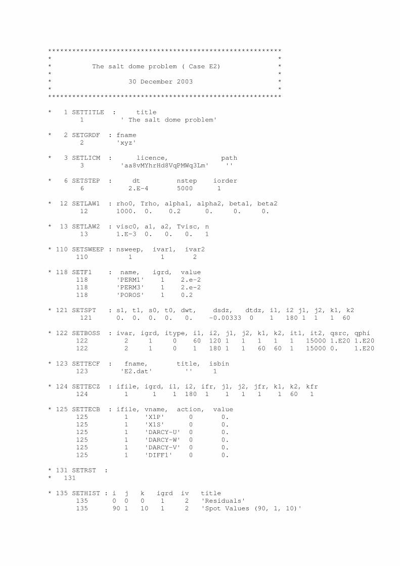
********************************************************** * * * The salt dome problem ( Case E2) * * * * 30 December 2003 * * * ********************************************************** * 1 SETTITLE : title 1 ' The salt dome problem' * 2 SETGRDF : fname 2 'xyz' * 3 SETLICM : licence, path 3 'aa8vMYhrHd8VqPMWq3Lm' '' * 6 SETSTEP : dt nstep iorder 6 2.E-4 5000 1 * 12 SETLAW1 : rho0, Trho, alpha1, alpha2, beta1, beta2 12 1000. 0. 0.2 0. 0. 0. * 13 SETLAW2 : visc0, a1, a2, Tvisc, n 13 1.E-3 0. 0. 0. 1 * 110 SETSWEEP : nsweep, ivar1, ivar2 110 1 1 2 * 118 SETF1 : name, igrd, value 118 'PERM1' 1 2.e-2 118 'PERM3' 1 2.e-2 118 'POROS' 1 0.2 * 121 SETSPT : s1, t1, s0, t0, dwt, dsdz, dtdz, i1, i2 j1, j2, k1, k2 121 0. 0. 0. 0. 0. -0.00333 0 1 180 1 1 1 60 * 122 SETBOSS : ivar, igrd, itype, i1, i2, j1, j2, k1, k2, it1, it2, qsrc, qphi 122 2 1 0 60 120 1 1 1 1 1 15000 1.E20 1.E20 122 2 1 0 1 180 1 1 60 60 1 15000 0. 1.E20 * 123 SETTECF : fname, title, isbin 123 'E2.dat' '' 1 * 124 SETTECZ : ifile, igrd, i1, i2, ifr, j1, j2, jfr, k1, k2, kfr 124 1 1 1 180 1 1 1 1 1 60 1 * 125 SETTECB : ifile, vname, action, value 125 1 'X1P' 0 0. 125 1 'X1S' 0 0. 125 1 'DARCY-U' 0 0. 125 1 'DARCY-W' 0 0. 125 1 'DARCY-V' 0 0. 125 1 'DIFF1' 0 0. * 131 SETRST : * 131 * 135 SETHIST : i j k igrd iv title 135 0 0 0 1 2 'Residuals' 135 90 1 10 1 2 'Spot Values (90, 1, 10)'

135 90 1 0 1 2 'Profiles, i = 90' * 136 SETHIST2 : igra vname label 136 1 'RESP' 'Pressure' 136 1 'RESS' 'Salinity' 136 2 'X1P' 'Pressure' 136 2 'X1S' 'Salinity' 136 3 'X1P' 'Pressure' 136 3 'X1S' 'Salinity' ********************************************************** * * * GRIDGEN setting * * 1004 GRGPCOS : icosp 1004 3 * 1005 GRGXDIS : x0, x1, x2, x3, nx1, nx2, nx3 1005 0. 0. 900. 900. 0 180 0 * 1006 GRGYDIS : y0, y1, y2, y3, ny1, ny2, ny3 1006 0. 0. 5. 5. 0 1 0 * 1007 GRGZDIS : z3, z4, z5, nz1, nz2, nz3, nz4, nz5 1007 0. -300. -300. 0 0 0 60 0 *********************************************************** * * NOTE: Problem scaled with a factor of 1.E13

********************************************************** * * * The floating island ( Case E5) * * * * 30 December 2003 * * * ********************************************************** * 1 SETTITLE : title 1 ' The floating island' * 2 SETGRDF : fname 2 'xyz' * 3 SETLICM : licence, path 3 'aa8vMYhrHd8VqPMWq3Lm' '' * 6 SETSTEP : dt nstep iorder 6 8.64E5 2000 1 * 12 SETLAW1 : rho0, Trho, alpha1, alpha2, beta1, beta2 12 1000. 0. 0.0078 0. 0. 0. * 13 SETLAW2 : visc0, a1, a2, Tvisc, n 13 2.E-3 0. 0. 0. 1 * 16 SETGWT : grlx, facmin 16 0.8 0.001 * 110 SETSWEEP : nsweep, ivar1, ivar2 110 1 1 2 * 115 SETTOP : ssea, tsea, tland 115 1.0 0. 0. * 118 SETF1 : name, igrd, value 118 'PERM1' 1 2.E-14 118 'PERM3' 1 2.E-12 118 'PERM4' 1 2.E-14 118 'DIFF1' 1 1.E-12 118 'DIFF3' 1 1.E-12 118 'DIFF4' 1 1.E-12 118 'POROS' 1 1.E-3 118 'GWT_FILL' 1 1. 118 'GWT_GH' 1 0. * 119 SETF2 : name, igrd, value, i1, i2, j1, j2, k1, k2 * 119 'PME' 1 3.17E-9 26 75 1 1 0 0 119 'PME' 1 1.58E-9 26 75 1 1 0 0 * 121 SETSPT : s1, t1, s0, t0, dwt, dsdz, dtdz, i1, i2, j1, j2, k1, k2 121 0. 0. 1. 0. 0. 0. 0. 1 100 1 1 1 50 * 122 SETBOSS : ivar, igrd, itype, i1, i2, j1, j2, k1, k2, it1, it2, qsrc, qphi 122 2 1 1 1 100 1 1 1 1 1 20000 0. 0. * 123 SETTECF : fname, title, isbin 123 'E5.dat' '' 0 * 124 SETTECZ : ifile, igrd, i1, i2, ifr, j1, j2, jfr, k1, k2, kfr 124 1 1 1 100 1 1 1 1 1 53 1

* 125 SETTECB : ifile, vname, action, value 125 1 'X1P' 0 0. 125 1 'X1S' 0 0. 125 1 'GWT_FILL' 0 0. 125 1 'DARCY-U' 0 0. 125 1 'DARCY-V' 0 0. 125 1 'DARCY-W' 0 0. * 131 SETRST : * 131 * 135 SETHIST : i j k igrd iv title 135 0 0 0 1 1 'Residuals' 135 50 1 49 1 1 'Spot Values (50, 1, 49)' 135 50 1 0 1 1 'Profile, i = 50' * 136 SETHIST2 : igra vname label 136 1 'RESP' 'Pressure' 136 1 'RESS' 'Salinity' 136 2 'X1P' 'Pressure' 136 2 'X1S' 'Salinity' 136 3 'GWT_FILL' 'Saturation' 136 3 'X1S' 'Salinity' ********************************************************** * * * GRIDGEN setting * * 1001 GRGTEC : fname, title, isbin 1001 'FItec' 'grid' 0 * 1003 GRGTOP : fname 1003 'USER' * 1004 GRGPCOS : icosp 1004 2 * 1005 GRGXDIS : x0, x1, x2, x3, nx1, nx2, nx3 1005 0. 0. 1000. 1000. 0 100 0 * 1006 GRGYDIS : y0, y1, y2, y3, ny1, ny2, ny3 1006 0. 0000. 10. 00. 0 1 0 * 1007 GRGZDIS : z3, z4, z5, nz1, nz2, nz3, nz4, nz5 1007 -100. -500. -500. 4 0 9 40 0 + 1, 1. + 2, 2. + 3, 3. + 4, 4. ********************************************************** * NOTES : * Analytical solution should be included ( see Case A1) * ----- * * Timestep is equal to 10 days * * Array-Lengths: conref=ni*nj*nk*5 fill=ni*nj*nk gh=ni*nj * conref is the saturated conductivity, fill is the saturatio * level in a cell and gh is the groundwater level

* * The coupled Pressure-Salinity solution should be tried. * * For rain=100 mm/year the fresh water lens reaches the bottom * boundary. May affect the simulation.

********************************************************** * * * Two-Fluid problem ( Case E6) * * * * 30 December 2003 * * * ********************************************************** * 1 SETTITLE : title 1 'Two Fluid Problem' * 2 SETGRDF : fname 2 'xyz' * 3 SETLICM : licence, path 3 'aa8vMYhrHd8VqPMWq3Lm' '' * 6 SETSTEP : dt nstep iorder 6 1.e2 100 1 * 9 SETF0: vname, igrd, val 9 'POROS' 1 1. 9 'PERM1' 1 1.E-12 9 'PERM3' 1 1.E-12 9 'CAPA' 1 2.E6 9 'TCOND1' 1 1.E-10 9 'TCOND3' 1 1.E-10 * 12 SETLAW1: rho0, Trho, alpha1, alpha2, beta1, beta2 12 1000. 10. 0.00 0. 5.e-3 0. * 13 SETLAW2 : visc0, a1, a2, Tvisc, n 13 2.E-3 0.2 0. 10 1 * 14 SETLAW3 : cp0, a1, a2 14 4200. 0. 0. * 110 SETSWEEP : nsweep, ivar1, ivar2 110 1 1 1 * 111 SETITC1 : nitc1, nvar3, nvar4 111 1 3 3 * 119 SETF2 : name, igrid, value, i1, i2, j1, j2, k1, k2 119 'X2T' 1 10. 1 80 1 1 1 40 119 'X2T' 1 20. 81 160 1 1 1 40 * 123 SETTECF : fname, title, isbin 123 'E6.dat' '' 1 * 124 SETTECZ : ifile, igrd, i1, i2, ifr, j1, j2, jfr, k1, k2, kfr 124 1 1 1 160 1 1 1 1 1 40 1 * 125 SETTECB : ifile, vname iaction value 125 1 'DARCY-U' 0 0. 125 1 'DARCY-V' 0 0. 125 1 'DARCY-W' 0 0. 125 1 'X1T' 0 0. 125 1 'X1P' 0 0. * 135 SETHIST : i j k igrd iv title
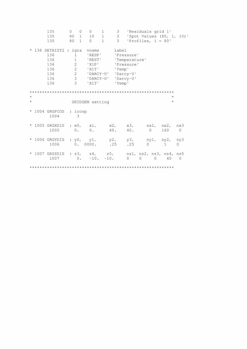
135 0 0 0 1 3 'Residuals grid 1' 135 80 1 10 1 3 'Spot Values (80, 1, 10)' 135 80 1 0 1 3 'Profiles, i = 80' * 136 SETHIST2 : igra vname label 136 1 'RESP' 'Pressure' 136 1 'REST' 'Temperature' 136 2 'X1P' 'Pressure' 136 2 'X1T' 'Temp' 136 2 'DARCY-U' 'Darcy-U' 136 3 'DARCY-U' 'Darcy-U' 136 3 'X1T' 'Temp' ********************************************************** * * * GRIDGEN setting * * 1004 GRGPCOS : icosp 1004 3 * 1005 GRGXDIS : x0, x1, x2, x3, nx1, nx2, nx3 1005 0. 0. 40. 40. 0 160 0 * 1006 GRGYDIS : y0, y1, y2, y3, ny1, ny2, ny3 1006 0. 0000. .25 .25 0 1 0 * 1007 GRGZDIS : z3, z4, z5, nz1, nz2, nz3, nz4, nz5 1007 0. -10. -10. 0 0 0 40 0 **********************************************************