dansgaard-oeschgercycles:interactionsbetweenoceanandseaice intrinsic to ... ·...

Dansgaard-Oeschger cycles: Interactions between ocean and sea iceintrinsic to the Nordic seas

Trond M. Dokken,1,2 Kerim H. Nisancioglu,1,2,3 Camille Li,2,4 David S. Battisti,2,5

and Catherine Kissel 6

Received 20 May 2013; revised 16 July 2013; accepted 16 July 2013.

[1] Dansgaard-Oeschger (D-O) cycles are the most dramatic, frequent, and wide-reachingabrupt climate changes in the geologic record. On Greenland, D-O cycles are characterizedby an abrupt warming of 10 ± 5°C from a cold stadial to a warm interstadial phase, followedby gradual cooling before a rapid return to stadial conditions. The mechanisms responsiblefor these millennial cycles are not fully understood but are widely thought to involve abruptchanges in Atlantic Meridional Overturning Circulation due to freshwater perturbations.Here we present a new, high-resolution multiproxy marine sediment core monitoringchanges in the warm Atlantic inflow to the Nordic seas as well as in local sea ice cover andinflux of ice-rafted debris. In contrast to previous studies, the freshwater input is found to becoincident with warm interstadials on Greenland and has a Fennoscandian rather thanLaurentide source. Furthermore, the data suggest a different thermohaline structure for theNordic seas during cold stadials in which relatively warmAtlantic water circulates beneath afresh surface layer and the presence of sea ice is inferred from benthic oxygen isotopes. Thisimplies a delicate balance between the warm subsurface Atlantic water and fresh surfacelayer, with the possibility of abrupt changes in sea ice cover, and suggests a novelmechanism for the abrupt D-O events observed in Greenland ice cores.

Citation: Dokken, T. M., K. H. Nisancioglu, C. Li, D. S. Battisti, and C. Kissel (2013), Dansgaard-Oeschger cycles:Interactions between ocean and sea ice intrinsic to the Nordic seas, Paleoceanography, 28, doi:10.1002/palo.20042.

1. Introduction

[2] There is a wealth of proxy data showing that the cli-mate system underwent large, abrupt changes throughoutthe last ice age. Among these are about one score large,abrupt climate changes known as Dansgaard-Oeschgerevents that occurred every 1–2 kyr. These events were firstidentified in ice cores taken from the summit of Greenland[Dansgaard et al., 1993; Bond et al., 1993] and are character-ized by an abrupt warming of 10 ± 5°C in annual averagetemperature [Severinghaus and Brook, 1999; Lang et al.,1999; NGRIP, 2004; Landais et al., 2004; Huber et al.,2006]. Subsequent observational studies demonstrated thatthe D-O events represent a near-hemispheric scale climateshift (see, e.g., Voelker [2002] and Rahmstorf [2002] for anoverview). Warming in Greenland is coincident with

warmer, wetter conditions in Europe [Genty et al., 2003],an enhanced summer monsoon in the northwest IndianOcean [Schulz et al., 1998; Pausata et al., 2011], a northwardshift of precipitation belts in the Cariaco Basin [Petersonet al., 2000], aridity in the southwestern United States[Wagner et al., 2010], and changes in ocean ventilation offthe shore of Santa Barbara, California [Hendy et al., 2002].Each abrupt warming shares a qualitatively similar tempera-ture evolution: about 1000 years of relatively stable coldconditions, terminated by an abrupt (less than 10 years) jumpto much warmer conditions that persist for 200–400 years,followed by a more gradual transition (~50 to 200 years)back to the cold conditions that precede the warming event.This sequence of climate changes is often referred to as aD-O cycle.[3] The leading hypothesis for D-O cycles attributes them

to an oscillation of the Atlantic Meridional OverturningCirculation (AMOC) [Broecker et al., 1985], with “on” and“off ” (or “weak”) modes of the AMOC [Stommel, 1961;Manabe and Stouffer, 1988] producing warm interstadialsand cold stadials, respectively, through changes in the merid-ional ocean heat transport. Indeed, interstadial and stadialconditions on the Greenland summit are associated withmarkedly different water mass properties (temperature andsalinity) in the North Atlantic [Curry and Oppo, 1997] andNordic seas [Dokken and Jansen, 1999]. Transitions betweenthe two phases are thought to arise from changes in the fresh-water budget of the North Atlantic [Broecker et al., 1990]. Inparticular, Birchfield and Broecker [1990] proposed that the

1UNI Research AS, Bergen, Norway.2Bjerknes Centre for Climate Research, Bergen, Norway.3Department of Earth Science, University of Bergen, Bergen, Norway.4Geophysical Institute, University of Bergen, Bergen, Norway.5Department of Atmospheric Sciences, University of Washington,

Seattle, Washington, USA.6Laboratoire des Sciences du Climat et de l’Envionnement, CEA/CNRS/

UVSQ, Gif-sur-Yvette, France.

Corresponding author: K. H. Nisancioglu, Department of Earth Science,University of Bergen, Allegaten 70, 5007 Bergen, Norway. ([email protected])

©2013. American Geophysical Union. All Rights Reserved.0883-8305/13/10.1002/palo.20042

1

PALEOCEANOGRAPHY, VOL. 28, 1–12, doi:10.1002/palo.20042, 2013

continental ice sheets covering North America and Eurasiawere the most likely sources for the freshwater [see alsoPetersen et al., 2013]. Abrupt events later during the deglaci-ation may have seen a contribution from Antarctica as well[Clark et al. 2001], but it is not clear that the underlyingmechanisms for these events are the same as for the D-Oevents occurring prior to the Last Glacial Maximum (21 kyr).[4] A number of studies with climate models of intermedi-

ate complexity (EMICs) have produced two quasi-stablephases in the AMOC by imposing ad hoc cyclic freshwaterforcing [Marotzke and Willebrand, 1991; Ganopolski andRahmstorf, 2001; Knutti et al., 2004]. Although these modelssimulate a temperature evolution on the Greenland summitthat is qualitatively similar to observations, the changes inthe simulated local and far-field atmospheric response aresmall compared to observations. Similar experiments withstate-of-the-art climate models produce local and far-fieldresponses that are in better agreement with the proxy data[e.g., Vellinga and Wood, 2002]. However, these modelsrequire unrealistically large freshwater perturbations, andon Greenland, the simulated stadial to interstadial transitionsare not as abrupt as observed. In both cases, the prescribedexternal forcing is ad hoc and yet is entirely responsible forthe existence and the longevity of the two phases (i.e., thecold phase exists as long as the freshwater forcing is applied).[5] Despite the unresolved questions surrounding D-O

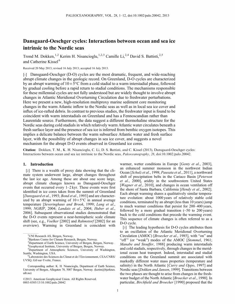
cycles, there has been progress. The direct, causal agent forthe abrupt climate changes associated with D-O warmingevents is thought to be abrupt reductions in North Atlanticsea ice extent [Broecker, 2000; Gildor and Tziperman,2003; Masson-Delmotte et al., 2005; Jouzel et al., 2005].Studies using atmospheric general circulation models(AGCMs) show that the local precipitation and temperatureshifts (inferred from oxygen isotopes and accumulationchanges) on the Greenland summit associated with a typicalD-O event are consistent with the response of the atmosphereto a reduction in winter sea ice extent, in particular in theNordic seas region (e.g., Figure 1) [see also Renssen andIsarin, 2001; Li et al., 2005, 2010]. Away from the NorthAtlantic, the northward shift of tropical precipitation belts as-sociated with D-O warming events mirrors the southwardshift simulated by coupled climate models in response to

freshwater hosing and expansion of sea ice [Vellinga andWood, 2002; Otto-Bliesner and Brady, 2010; Lewis et al.,2010] and by AGCMs coupled to slab ocean models inresponse to a prescribed expansion of North Atlantic sea ice[Chiang et al., 2003], thus supporting the existence of arobust link between North Atlantic sea ice cover and far-field climate.[6] More recently, a number of studies have shown that

cold stadial conditions are associated with subsurface and in-termediate depth warming in the North Atlantic [Rasmussenand Thomsen, 2004; Marcott et al., 2011]. This subsurfacewarming may have bearing on many aspects of D-O cycles,from the abruptness of the warming (stadial-to-interstadial)transitions [Mignot et al., 2007] to the possibility of ice shelfcollapses during D-O cycles [Ãlvarez-Solas et al., 2011;Marcott et al., 2011; Petersen et al., 2013].[7] In this study, we focus on the subsurface warming

rather than ice rafting to build physical arguments for themechanisms behind D-O cycles. Changes in sea ice and sub-surface ocean temperatures during D-O transitions are linkedto each other by the ocean circulation and to changes inGreenland by the atmospheric circulation. To elucidate theselinks requires marine records that (i) are situated in keyregions of the North Atlantic, (ii) are representative of condi-tions through the depth of the water column, and (iii) can becompared to records of atmospheric conditions (as measuredfrom the Greenland summit) with a high degree of certaintyin terms of timing. In addition, because of the abruptness ofthe transitions (on the order of decades or less), the marinerecords must be of exceptionally high resolution.[8] Here we present new data from a Nordic seas core that

meet these criteria. The core site is strategically located in theAtlantic inflow to the Nordic seas, where extremely high sed-imentation rates allow for decadal-scale resolution of bothsurface and deepwater proxies. In addition to an age modelbased on calibrated carbon-14 ages and magnetic properties,ash layers provide an independent chronological frameworkto synchronize signals in the marine core with signals in anice core from the summit of Greenland.[9] The new marine proxy data reveal systematic changes

in the hydrography of the Nordic seas as Greenland swingsfrom stadial (cold) to interstadial (warm) conditions and back

Figure 1. Surface air temperature response during the extended winter season (December–April) tochanges in Nordic seas ice cover (figure redrawn from simulations in Li et al. [2010]). Black contoursindicate maximum (March) ice extent in the two scenarios. The white dot is the location of our coreMD992284.

DOKKEN ET AL.: D-O CYCLES AS SEEN IN THE NORDIC SEAS

2

through several D-O cycles, with details of the transitionsbetter resolved than in any previously studied core. The inter-stadial phase in the Nordic seas is shown to resemble currentconditions, while the stadial phase has greatly enhanced seaice coverage (as inferred from benthic oxygen isotopes) anda hydrographic structure similar to that in the Arctic Oceantoday. The variations recorded by the marine proxies nearthe transitions are used to determine the possible mechanismsthat cause the North Atlantic climate system to jump abruptlyfrom stadials to interstadials and to transition slowly backfrom interstadials to stadials. In a departure from mostexisting hypotheses for the D-O cycles, the conceptual model

presented here does not require freshwater fluxes from icesheets to enter the ocean at specific times during the D-O cy-cle [e.g., Birchfield and Broecker, 1990; Petersen et al.,2013]. Rather, it relies on ocean-sea ice interactions internalto the Nordic seas to trigger stadial-interstadial transitions.[10] The paper proceeds as follows. Section 2 contains a

description of the marine sediment core, analysis methods,the construction of the age model for the core, and the con-struction of a common chronology with an ice core fromthe summit of Greenland. Section 3 describes the cold stadialand warm interstadial climate of the Nordic seas as seen inthe marine sediment data. Section 4 analyzes the relevance

a

b

c

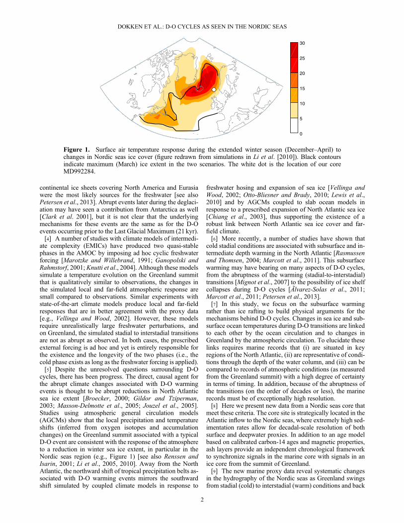
Figure 2. (a) δ18O of NGRIP plotted versus time (in kyr). (b) Measured low-field magnetic susceptibility,anhysteretic remanent magnetization (ARM) (log scale/unit 10�6 A/m) in MD992284 plotted versus depth.Red stars indicate the stratigraphical level (depths) from where AMS 14C ages are measured (see alsoTable 1). (c) NGRIP δ18O (black line) and ARM (blue line) record from MD992284 after converting theMD992284 age to the NGRIP age (b2k). Green vertical lines indicate tuning points for the (numbered) on-set of interstadials in the ice core and marine records. Red vertical lines connect identical ash layers(FMAZIII and FMAZII) in NGRIP and MD992284 as described in the text and in Table 1.


3

of the new proxy data for the D-O cycles as observed onGreenland and, in particular, the mechanisms behind theabrupt transitions. Section 5 presents a summary of the re-sults and a discussion of the implications.

2. Materials and Methods

[11] Core MD992284 was collected in the Nordic seas dur-ing the MD114/IMAGES V cruise aboard R/V MarionDufresne (IPEV) at a water depth of 1500m on the northeast-ern flank of the Faeroe-Shetland channel. The core is strategi-cally located in the Atlantic inflow to the Nordic seas and hasan exceptionally high sedimentation rate, allowing fordecadal-scale resolution of both surface and deep water prox-ies. The unique, high-resolution marine core with a wellconstrained age model (Figure 2) shows evidence for system-atic differences in the Nordic seas during Greenland intersta-dials versus Greenland stadials. These new data are used tocharacterize the important hydrographic features of theNordic seas in each of these two phases of the D-O cycle aswell as the transition between the phases.[12] Figure 2a shows a segment of the North Greenland Ice

Core Project (NGRIP) ice core from Greenland [NGRIP,2004] during late Marine Isotope Stage 3 (MIS3) containingseveral typical D-O cycles. To compare the marine record tothe ice core record, we have constructed an age model bymatching rapid transitions in MD992284 to NGRIP usingthe Greenland Ice Core Chronology 2005 (GICC05)[Svensson et al., 2006] and ash layers found in both cores.The common chronology allows the Nordic seas data to belinked directly to Greenland ice core signals.

2.1. Age Model for Marine Sediment Core

[13] Age models based on the ice core and calibrated 14Cdates can be used to estimate “true ages” for the marine corebut will be subject to errors due to missing or misinterpretedice layers, uncertainty in reservoir ages, and uncertainty insedimentation rates. Our approach here is thus not to relyon true ages, but rather on a stratigraphic tuning of the marinerecord to the ice core record. We use the high-frequency var-iations in measured anhysteretic remanent magnetization(ARM) during Marine Isotope Stage 3 (MIS3) in the marinecore (Figure 2b). The fast oscillations in magnetic propertiesduring MIS3 in the North Atlantic/Nordic seas have beenshown to be in phase with changes in δ18O of Greenlandice cores [Kissel et al., 1999]. We use the ARM record fortuning only, with no further subsequent paleoproxy interpre-tation of this parameter. The tuning has been performed usingthe tuning points as indicated in Figure 2 and the softwarepackage AnalySeries 2.0 [Paillard et al., 1996].[14] A final step in the synchronization between the ice

core and the marine core is done with tephra layers. Twoash zones identified in the marine record have also been iden-tified in the NGRIP ice core [Svensson et al., 2008], theFugloyarbanki Tephra (FMAZII) [Davies et al., 2008] andFareo Marine Ash Zone III (FMAZIII) [Wastegård et al.,2006]. These ashes allow for a direct, independent compari-son between the marine and ice core records. Our chronologyplaces the ash layer FMAZIII less than 100 years after theonset of interstadial 8 in NGRIP (see Figure 2) and thus pro-vides a verification of the initial tuning of the ARM record inMD992284 to the δ18O record in NGRIP. These two ash

layers are also used as tuning points in the final age model.The final age model gives the best possible synchronizationof the marine record to the NGRIP ice core record [NGRIP,2004], making it possible to determine the relative timingof observed changes in the marine proxies compared to tem-perature changes on Greenland.[15] The final tuned age model presented for MIS3

(Figure 3) only uses the ages given by the tuning to NGRIPand the ash layers. As an independent check, we note thatthe new age model for the marine sediment core is consistentwith calibrated 14C dates (Table 1). These are calculatedusing the calibration software CALIB 6.0 [Stuiver andReimer, 1993] and an ocean reservoir age of 400 years, ap-plying the “Marine09” calibration curve [Hughen et al.,2004] for ages younger than 25 kyr B.P. (14C age, kilo yearsbefore present) and the “Fairbanks0107” calibration curvefor anisotropy of magnetic susceptibility (AMS) 14C samplesof ages older than 25 kyr B.P. [Fairbanks et al., 2005].Offsets of at least a few thousand years from the true ageare expected due to the relatively large error in 14C measure-ments in the interval of 30–40 kyr B.P., as well as errors intransformation from 14C ages to calibrated ages. Additionalerror is introduced by the assumption that sedimentation ratesare constant between the dated levels.

2.2. Near-Surface Ocean Temperature Estimates

[16] For the planktonic foraminifera, raw census data of theplanktonic assemblages were analyzed and the transfer func-tion technique (maximum likelihood (ML)) was used tocalculate near-surface temperature. The ML method operateswith a statistical error close to ±1°C and is found to give theleast autocorrelation compared to other statistical methods[Telford and Birks, 2005].

2.3. Transforming the δ18O Into a Measure of SeawaterIsotopic Composition

[17] The ratio of oxygen-18 to oxygen-16 as they are incor-porated into foraminiferal calcite (δ18Ocalcite) is dependent onboth seawater δ18O (expressed as per mil deviations fromVienna Standard Mean Ocean Water (SMOW)) and calcifica-tion temperature. Foraminifera-based SST estimates providean independent estimate of the calcification temperature andtherefore the temperature effects on calcite δ18O.[18] The temperature to δ18O calibration used is based on

Kim and O’Neil [1997]:

T ¼ 16:1� 4:64 δ18Ocalcite � δ18OSMOW

� �

þ 0:09 δ18Ocalcite � δ18OSMOW

� �2

[19] Knowing the calcification temperature (T) from theforam transfer function and the measured δ18Ocalcite, wecan extract the isotopic composition of the ambient seawater (δ18OSMOW). The relationship between salinity andδ18OSMOW in the ocean depends on the spatial variation ofδ18O associated with the fresh water flux to the ocean, theamount of seawater trapped in ice caps, as well as ocean circu-lation [Bigg and Rohling, 2000].[20] Before translating glacial δ18O data into a measure of

δ18OSMOW, the effect of global ice volumemust be accountedfor. Fractionation processes of oxygen isotopes when water


4

freezes into ice produce an ocean-wide δ18O shift of about0.1‰ per 10m of sea level stored in continental ice sheets[Fairbanks, 1989]. A review of recent advances in the esti-mates of sea level history during MIS3 is given by Siddallet al. [2008]. The estimated sea level changes during MIS3vary in amplitude and timing between the different reconstruc-tions. In our study, we use the sea level reconstruction of

Waelbroeck et al. [2002], which fits well with availablecoral-based estimates for MIS3, to remove the effects ofchanging ice volume on the δ18O of ocean water. Note thatthe sea level correction is only applied to the planktonicδ18O data. In the benthic record, the gradual decrease in sealevel as well as a general cooling toward the Last GlacialMaximum is seen as a long term trend in the δ18O (Figure 3d).

Figure 3. Down core data sets fromNGRIP andMD992284 covering the period 41 to 31 ka plotted on theGICC05 (b2k) time scale. (a) NGRIP δ18O (proxy for Greenland temperature), (b) MD992284reconstructed temperature based on planktonic foram assemblages, (c) MD992284 near-surfaceδ18OSMOW, (d) MD992284 benthic δ18O, (e) MD992284 flux-corrected ice-rafted debris (IRD), (f)MD992284 near-surface δ13C, and (g) MD992284 benthic δ13C. Interstadial periods are indicated by greyshading. The near-surface δ18OSMOW is determined from theKim and O’Neil [1997] calibration curve usingthe δ18O of N. pachyderma sin. and the temperature obtained using transfer functions (see section 2). Thenear-surface δ13C is measured on N. pachyderma sin. and the benthic δ18O and δ13C are measured onCassidulina teretis.


5

2.4. Interstadial and Stadial Phases of a D-O Cycle

[21] Positioned in the path of inflowing warm Atlantic wa-ter to the Nordic seas and close to the routing of freshwaterfrom the Fennoscandian ice sheet, our marine sediment coreis ideally suited to better understand the changes to the hy-drography and sea ice cover of the Nordic seas duringMIS3. The use of an accurate age chronology constrainedby common tephra layers located at key transitions in the ma-rine and ice cores makes it possible to compare individualstadial and interstadial periods between the two climate ar-chives. Here we will describe the warm and cold phases ofD-O cycles as seen in the new Nordic seas sediment core dataand compare them to the Greenland ice core record before ex-amining the transitions in section 4.

2.5. The Nordic Seas During Greenland Stadials

[22] Foraminiferal assemblages used to reconstruct near-surface ocean temperature show that water masses at the coresite in the Nordic seas are ~2°Cwarmer during cold Greenlandstadials than during warm interstadials (Figure 3b). Further,there is a warm overshoot at the onset of each interstadial.Despite difficulties in acquiring reliable low-temperaturereconstructions in polar and Arctic water masses [e.g.,Pflaumann et al., 2003; Meland et al., 2005], the estimatedhigher temperatures during stadials compared to interstadialsare a robust result. This is based on higher percentagesof “Atlantic species” associated with relatively warm condi-tions (such as Globigerina bulloides, Neogloboquadrinapachyderma (dextral), and Turborotalita quinqueloba) andaccounting for ~20–30% of the total planktonic assemblageduring stadials. Interstadials are instead dominated by cold wa-ter (Arctic) species such as Neogloboquadrina pachyderma(sinistral), which account for nearly 100% of the total plank-tonic assemblage.[23] Planktonic foraminifera are known to change their

depth habitat in Arctic environments to avoid the low-salinitysurface, which is separated from the subsurface warmAtlantic layer by a halocline (strong vertical salinity gradi-ent). This results in different depth distributions of foraminif-era under different hydrographic conditions [Carstens et al.,1997]. Therefore, a reasonable interpretation of these data isthat, during cold stadials in the Nordic seas, the planktonicassemblages are located below the fresh surface layer andthus record the relatively warm temperatures just below thehalocline (Figure 4, left). At these depths, the foraminifera

are in contact with relatively warm Atlantic water that isisolated from the atmosphere by the halocline and sea icecover, both of which are features of the stadial phase of theD-O cycle. Note that at the end of each stadial phase, thereis a warm overshoot that provides a clue to understandingthe stadial-to-interstadial transition (discussed in section 4).[24] Combining stable isotope (δ18Ocalcite) measurements

on the planktonic foraminifera N. pachyderma sin. with theocean temperature reconstruction produces an estimateof the isotopic composition of sea water (δ18OSMOW).δ18OSMOW is partly related to salinity, but it also reflects spa-tial shifts in water masses. The isotopic composition of polarwater may be different compared to water of subtropical ori-gin, but because the planktonic foraminifera prefer to staywithin the warm Atlantic layer, we do not expect that themean δ18OSMOW (salinity) at the core site will be substan-tially different during stadials compared to interstadials.Indeed, we see in Figure 3c that there is no systematic differ-ence in the mean δ18OSMOW during stadial and interstadialperiods. The common near-surface temperature spikes at

Figure 4. A schematic column model of the (left) stadialand (right) interstadial phases consistent with the Nordicsea sediment core MD992284.

Table 1. Radiocarbon-Dated Intervals Used as a First Approximation to Create the Age Modela

Laboratory Referenceand Ash Identity

Mean Depth(cm)

14C Age, Uncorrected(yr B.P.)

Error,1σ(yr)

Calibrated Ages -Intercept (kyr)

Max. 1σ CalibratedAge (yr B.P.)

Min. 1σ CalibratedAge (yr B.P.)

TUa-3310 1,100.5 21,975 160 24.64 25,018 24,270FMAZ II 1,407.5 26.69 (b2k)POZ-29522 2,106.5 29,100 240 34.06 33,770 34,350POZ-29523 2,324.5 29,900 600 34.87 34,260 35,480POZ-17620 2,775.5 29,920 240 35.5 36,000 35,000POZ-17621 2,996.5 32,500 300 37.5 37,800 37,100FMAZ III 3,040.5 38.07 (b2k)POZ-29524 3,075.5 34,600 700 39.53 38,830 40,230

aAll AMS 14C ages are measured on N. pachyderma sin. Also shown in the table are two identified ash layers. The ages given for Fugloyarbanki Tephra(FMAZII) and Faroe Marine Ash Zone III (FMAZIII) are from Svensson et al. [2008]. The ash ages are referred to in b2k (before year A.D. 2000). Sampleswith laboratory reference “TUa-” are measured at the Uppsala Accelerator in Sweden, but the samples have been prepared at the radiocarbon laboratory inTrondheim, Norway. Samples labeled “POZ-” are prepared and measured in the radiocarbon laboratory in Poznan, Poland.


6

the transitions between stadial and interstadial phases and theconsistent near-surface temperature trends within the stadialand interstadial periods provide insight into the transitionmechanisms and are discussed in section 3.1.[25] The benthic δ18O record measured on Cassidulina

teretis (Figure 3d) is remarkably similar to the NGRIP re-cord, exhibiting the characteristic shape and abrupt transi-tions of D-O cycles. One explanation for the link betweenthe benthic δ18O and NGRIP is provided by Dokken andJansen [1999], who presented evidence that there are two dif-ferent forms of deep water production in the Nordic seas dur-ing the last glacial period, depending on the sea ice coverage.As in the modern climate, there is deep open ocean convec-tion in the Nordic seas during the last glacial period whenthe surface is free of sea ice. When Greenland is cold (thestadial phase of the D-O cycle), however, they argued thatthe benthic δ18O becomes lighter in the deep Nordic seasbecause there is sea ice formation along the Norwegian con-tinental shelf, which creates dense and isotopically light brinewater that is subsequently transported down the continentalslope and injected into the deeper water. In this scenario,the close link between the benthic δ18O record and NGRIPis due to the deep water being affected by continuous seaice formation throughout the stadial phase and by open oceanconvection during the interstadial phase of the D-O cycle.This interpretation of the benthic record is commensuratewith all of the other proxy data in Figure 3, which indicatesthat during the stadial phase of the D-O cycle, the Nordic seaswere covered with sea ice and the surface waters were fresh(Figure 3c) and at the freezing point. Further evidence forthe existence of extensive sea ice stems from Figure 3a andmodeling work that links the Greenland δ18O record to seaice extent in the Nordic seas (see section 1).[26] An alternative interpretation of benthic δ18O at nearby

core sites attributes the changes to bottom water temperaturerather than brine [Rasmussen and Thomsen, 2004]. Thetemperature change that would be required to explain the 1–1.5‰ shifts seen in benthic δ18O at our site implies a 4–6°Cwarming at a depth of 1500m during stadials and almost twiceas much during Heinrich events [e.g., Marcott et al., 2011].We believe that enhanced brine rejection at the surface andmoderately increased temperatures at depth act together to cre-ate the light benthic δ18O values during stadials and that bothprocesses are necessary for maintaining stadial conditions.[27] The record of ice-rafted debris (IRD) indicates that

there is less frequent ice rafting during cold stadial periodson Greenland (Figure 3e). In this core, the IRD is ofScandinavian origin, and the record implies that there is lesscalving from the Fennoscandian ice sheet during the coldstadial and therefore less meltwater derived from icebergs.Note that there are two Heinrich events during the time inter-val shown in Figure 3 (denoted H3 and H4 in Figure 3), bothof which occurred during the latter part of a cold stadial phaseof a D-O cycle. In this study, we are not concerned with theinfrequent, large Heinrich ice rafting events and do notconsider Heinrich events to be fundamental to the physicsof a D-O cycle. Instead, the reader is referred to the studyof Ãlvarez-Solas et al. [2011] for a discussion of the possiblerelationship between these two phenomena.[28] In general, the planktonic δ13C exhibits more negative

values during stadials (Figure 3f), suggesting that the water atthe preferred depth for the planktonic foraminifera is isolated

from the atmosphere. Thus, benthic and planktonic datacollectively suggest that during the stadial phase of the D-Ocycle, the eastern Nordic seas are characterized by extensivesea ice cover, a surface fresh layer separated by a haloclinefrom warmer, saltier subsurface waters, and by deep waterproduction by brine rejection along the Norwegian coast.

2.6. The Nordic Seas During Greenland Interstadials

[29] In the interstadial phase of the D-O cycle, whenGreenland is warm (Figure 3a), the Nordic seas are thoughtto be mostly free of sea ice. Without the presence of sea iceand an associated fresh surface layer, the water column isweakly stratified and the incoming Atlantic water efficientlyreleases heat to the atmosphere, as is the case in today’sNordic seas (Figure 4, right). As a consequence, subsurfacetemperatures in the Nordic seas are found to be relativelycold (Figure 3b), and any fresh water that may be depositedin the surface layer is easily removed by strong wind mixing,particularly during the winter.[30] As shown by Li et al. [2005], reduced North Atlantic

sea ice cover can account for the warm temperatures ob-served in the Greenland ice cores during interstadials of thelast glacial cycle (Figure 1). Due to the exceptional chronol-ogy of the high-resolution marine sediment record, we canconfidently link the timing of warm interstadial conditionson Greenland to periods in the marine record with high ben-thic δ18O (Figure 3d) and well-ventilated conditions in theNordic seas as evidenced by planktonic δ13C (Figure 3f).The high benthic δ18O values indicate less efficient brine for-mation combined with lower temperatures, supporting thepresence of reduced sea ice cover during interstadials in theNordic seas [Dokken and Jansen, 1999]. Note that the ben-thic δ13C record (Figure 3g) is not as straightforward to inter-pret as the planktonic δ13C record: the strong overshoot seenduring the transitions between stadial and interstadial condi-tions is discussed in detail in section 3.2.

3. Implications for D-O Cycles

3.1. Transition Between Stadial and Interstadial Phases

[31] The records presented thus far support the idea of areorganization of the vertical thermohaline structure of theNordic seas between the stadial and interstadials phases ofD-O cycles. In the interstadial phase, conditions in theNordic seas resemble those existing today: the heat transportedinto the region by the ocean and stored seasonally in the mixedlayer is released to the atmosphere, resulting in a moderate,seasonal sea ice cover. In the stadial phase, however, condi-tions in the Nordic seas resemble those existing in the ArcticOcean today: there is a fresh surface layer buffered from thewarm Atlantic water below by a halocline. In essence, thereis an expansion of sea ice southward from the Arctic into theNordic seas. Indeed, the stratification and vertical structureof the Nordic seas inferred from our proxy data (Figures 3and 4) are similar to those of today’s Arctic, where water isseveral (~3°C) degrees warmer at a depth of 400–500m thanat the surface in winter [e.g., Rudels et al., 2004].[32] During the stadial phase, the planktonic foraminfera

are mainly recording the temperature of water within, or justbelow, the halocline (Figure 4, left). The sea ice coverprevents wind mixing, and sea ice formation along theNorwegian coast creates dense brines that are rejected from


7

the surface and injected deeper in the water column, thus help-ing to maintain the halocline. As the stadial phase progresses,the planktonic foraminfera show an increase in temperature(Figure 3b) consistent with their depth habitat being continu-ously fed by the northward advection of relatively warm andsalty Atlantic water. With no possibility of venting heat tothe atmosphere above, because of extensive sea ice cover,the warming due to the inflow of warm Atlantic water gradu-ally reduces the density of the subsurface waters and weakensthe stratification that allows the halocline and sea ice cover toexist. The transition to warm interstadial conditions onGreenland occurs when the stratification and halocline weakento the point of collapse, at which point heat from the subsur-face layer is rapidly mixed up to the surface, melting backthe sea ice.[33] The removal of sea ice in the Nordic seas allows effi-

cient exchange of heat between the ocean and the atmosphereand is seen as an abrupt warming (D-O event) of 10 ± 5°C inGreenland at the start of each interstadial [NGRIP, 2004](Figure 1). There is a distinct overshoot (<100 years long)in foraminifera-derived subsurface temperatures right at thetransition (Figure 3b). The planktonic foraminifera live atthe interface between the surface and subsurface layers andimmediately feel the temperature effect as warm subsurfacewater is mixed up to the surface. Once the fresh surface layerhas been mixed away, the ocean is able to vent heat to theatmosphere. The foraminifera now find themselves living ina new habitat, an unstratified surface layer, which is colderthan their subsurface stadial habitat.[34] Once in the interstadial (Figure 4, right), conditions are

comparable to those of today: the Nordic seas are relatively icefree, inflowing warm Atlantic water is in contact with thesurface, and there is an efficient release of heat to the atmo-sphere. The planktonic-based temperatures show little change(Figure 3b), but there is a consistent reduction in salinity, inparticular, toward the end of each interstadial (Figure 3c).This freshening of the upper part of the Nordic seas water col-umn is most likely due to melting and calving of the nearbyFennoscandian ice sheet in response to the warm climate con-ditions, as is supported by the increased frequency of IRD de-posits at the site toward the end of each interstadial (Figure 3e).

3.2. Supporting Evidence From δ13C[35] The carbon isotope data from planktonic (N.

Pachyderma sin.) and benthic (C. teretis) foraminifera at thesite (Figures 3f and 3g) give additional clues about the transi-tion between stadial and interstadial phases in the Nordic seas.The isotopic signature of carbon (δ13C) preserved in the cal-cium carbonate shells of foraminfera is related to ventilationand water mass age: at the surface, CO2 exchange with theatmosphere and marine photosynthesis preferentially extract12C from seawater, causing enrichment of surface water indissolved inorganic 13C.When the water mass is isolated fromthe surface mixed layer, its δ13C value decreases with age dueto mixing with different water masses and gradual decomposi-tion of low δ13C organic matter. Although the benthic forami-nifera C. teretis do not live directly on the surface of themarine sediments, evidence from studies in the Nordic seasshows that the δ13C of C. teretis tracks the δ13C recorded byepibenthic species (benthic fauna living on top of the sedimentsurface at the seafloor). In the absence of epibenthic foraminif-era in high-deposition regions such as the core site, C. teretiscan be used with caution to infer past changes in deep waterδ13C [Jansen et al., 1989].[36] In the stadial phase, with extensive sea ice, relatively

young water of Atlantic origin with high δ13C (Figure 3f) en-ters the Nordic seas below the fresh surface layer and halo-cline. At the onset of the interstadial, there is a brief periodwith extremely light benthic δ13C (Figure 3f). This is consis-tent with a mixing in of old, poorly ventilated deep watermasses of Arctic origin from below the Atlantic layer in theNordic seas [e.g., Thornalley et al., 2011]. Enhanced mixingat the transition will also bring well-ventilated waters withhigh δ13C down from the surface; however, this signal isoverwhelmed by the mixing in of the old water from belowwith extremely light δ13C.[37] Early in the interstadial phase, following the abrupt

transition, the core site is dominated by high δ13C as seenin both the benthic (Figure 3f) and planktonic (Figure 3e) re-cords. At this point, the Nordic seas are free of sea ice andwell ventilated, and the stratification is weak due to efficientwinter mixing and absence of a halocline. Continuous inputof terrestrial freshwater from the Fennoscandian continentalso contributes to the high planktonic δ13C. However, to-ward the end of the interstadial, the influence of sea ice is in-creasing in the Nordic seas (Figure 3d) and the stratificationis increasing, as evidenced by decreasing surface salinity(Figure 3b). As a consequence, benthic δ13C is reduced(Figure 3f ), indicating increased stratification and less venti-lation of waters at the depth of the core site.[38] Returning to the stadial phase (Figure 5), with an

extensive sea ice cover and return of the halocline, thesurface and intermediate waters are now isolated fromthe atmosphere, as evidenced by relatively low planktonicδ13C values (Figure 3e). Although the qualitative featureswe have described are robust for each D-O cycle, thereare quantitative differences between each cycle. For exam-ple, convection may reach deeper during some interstadialsthan others, making the light spike more pronounced, or theocean may restratify more quickly during some interstadials,resulting in a more immediate recovery to heavier δ13Cvalues. Such differences will also be reflected in the otherproxy records.

Figure 5. A schematic timeline showing the evolution of aD-O cycle that is consistent with the Nordic sea sedimentcore MD992284 and the NGIP ice core.


8

4. Discussion

[39] The conceptual model for D-O cycles presented in theprevious section and summarized in Figures 5 and 6 is basedon the proxy records measured in MD992284 and specificallyon the relationship between signals in these high-resolutionmarine records and signals in the Greenland oxygen isotoperecord. The marine records themselves provide direct informa-tion on the water column in the Atlantic inflow region of theNordic seas. However, the expected changes in sea ice coverillustrated in the conceptual model have implications for theresponse and role of other parts of the climate system in D-Ocycles. We have focused on the Greenland oxygen isotope re-cord as a reference time series for D-O cycles, but additionalinformation is provided by the Greenland deuterium excessrecord [Jouzel et al., 2005; Masson-Delmotte et al., 2005;Thomas et al., 2009]. Deuterium excess shows a rapid de-crease in the temperature of source waters for Greenland pre-cipitation at stadial to interstadial transitions. Assuming thatthe abrupt transition from stadial to interstadial conditions is

mediated by the removal of sea ice in the Nordic seas, thiswould provide a new, local source of moisture for precipitationon the Greenland ice sheet during warm interstadials. Theocean temperature of this source would be significantly lowerthan sources farther to the south [Sachs and Lehman, 1999],thus explaining the observed 3°C rapid decrease in the sourcetemperature for precipitation on Greenland during phases ofrapid increase in surface air temperature of D-O cycles[Steffensen et al., 2008].[40] On a larger scale, changes in sea ice cover are

expected to be associated with a reorganization of atmo-spheric circulation, as is suggested by changes in dust deliv-ered to Greenland [Mayewski et al., 1997]. We hypothesizethat during interstadials, the storm track extends northeast-ward into the Nordic seas, transporting heat into the regionand inhibiting formation of sea ice by mechanical mixing.During stadials, the storm track is more zonal and positionedsouth of the Fennoscandian ice sheet. Experiments with anatmospheric general circulation model forced by variouscontinental ice sheet [Li and Battisti, 2008] and sea ice

Figure 6. Schematic showing wintertime conditions in the North Atlantic and Nordic seas during typical(left) cold stadial periods and (right) warm interstadial periods of a D-O cycle. (top) Maps of the NorthAtlantic region with sea ice extent and land ice. The location of the sediment core is marked with a blue dot,and the sections described in the bottom panels are indicated. (middle) locations A and C show north-southsections of the North Atlantic during stadial and interstadial conditions, respectively. (bottom) Locations Band D show east-west sections of the Norwegian Sea during stadial and interstadial conditions, respectively.


9

configurations [Li et al., 2010] show that a southwarddisplaced jet is also associated with a more quiescent stormtrack, which would be more conducive to sea ice productionin the Nordic seas and with the occurrence of katabatic windscoming off the Fennoscandian ice sheet. In turn, this wouldpromote sea ice production in leads and polynyas on the con-tinental shelf. Shifts in the orientation of the Atlantic stormtrack could help explain the dust record in Greenland, as wellas far-field monsoon and precipitation changes associatedwith D-O cycles [Pausata et al., 2011].[41] Many previous models of D-O cycles require, or as-

sume, a flux of freshwater to the North Atlantic mainly fromthe Laurentide ice sheet in order to maintain extensive sea icecover over the Nordic seas during stadials. In contrast, theprovenance of IRD in MD992284 indicates that the freshwa-ter forcing originates from the Fennoscandian ice sheet and isassociated with interstadials as much as, if not more than,stadials. This provides a local freshwater source in the pathof the Atlantic inflow in a highly sensitive area of theNordic seas, which can aid more directly in creating a halo-cline and facilitating expansion of sea ice compared to fresh-water sources on the western rim of the North Atlantic.[42] We further expect that the presence of a halocline and

extensive sea ice during stadials greatly reduces the ventilationof the deep ocean as it prevents contact between inflowingAtlantic water and the atmosphere in the Nordic seas. This willimpact the properties of the return flow of Atlantic water leav-ing the Nordic seas and should be recorded by intermediateand deepwater proxies throughout MIS3. The marine proxydata presented in this study support the existence of an activecirculation of relatively warm Atlantic water into the Nordicseas during stadials but do not give a direct measure of the rateof Atlantic meridional overturning circulation. Evaluatingchanges in the AMOC as a response to enhanced stratificationin the Nordic seas during stadials is beyond the scope of thisstudy. However, such changes are expected, as the returningoutflow of Atlantic water from the Nordic seas would not besufficiently dense to sink into the deep abyss during stadials.As discussed in several studies [Crowley, 1992; Stocker andJohnsen, 2003], a reduction in the AMOC could lead towarming of the Southern Ocean and possibly explain the “see-saw” pattern with warm temperatures on Antarctica whenGreenland is cold [EPICA, 2006; Blunier and Brook, 2001].[43] MIS3 records from other Nordic seas marine cores

share many consistent features with the records presented inthis study. However, different interpretations of these fea-tures lead to hypothesized mechanisms for D-O cycles thatare different from ours in important ways. For example,Rasmussen and Thomsen [2004] suggest that there iswarming at depth during stadials, based on the depleted ben-thic δ18O from a sediment core obtained from the centralNordic seas basin at 1000m depth. We also observe depletedbenthic δ18O during stadials at our core site, but we interpretthis primarily to be due to brine production. Given the posi-tion of our core on the Norwegian slope, interpreting thedepleted benthic δ18O exclusively as a temperature signalwould imply temperatures of 4–6°C warmer during stadialperiods at a depth of 1500m in the Nordic seas, which wefind unlikely.[44] Another example, Petersen et al. [2013] hypothesize

that the duration of the interstadial and stadial phases of theD-O cycles is related to ice shelves, while sea ice changes

provide the abrupt transitions. Critical support for this iceshelf mechanism is an increase in ice rafting during eachD-O stadial inferred from IRD and fresh surface anomaliesbased on planktonic δ18O [Dokken and Jansen, 1999; vanKreveld et al., 2000; Elliot et al., 1998, 2001]. The postulatedoccurrence of ice rafting during cold Greenland stadials, asrequired by the Petersen et al. [2013] hypothesis, appearsto disagree with the chronology of our marine sediment core,in which ice rafting is enhanced during the latter part of theinterstadials (Figure 3e). However, Petersen et al. [2013] fo-cus on the Irminger Basin, which is far enough away fromour core site that there may be no inconsistency. Note alsothat in the earlier studies, using cores with a lower sedimen-tation rate, there is hardly any sedimentation during stadials,leaving nearly only coarse-grained lithic content. This couldindicate that the fraction of coarse- to fine-grained sedimentis not solely due to changes in iceberg calving, but couldpartly be due to reduced sedimentation rates and runoff dur-ing the cold stadial periods when the Nordic seas are thoughtto be covered by extensive sea ice.[45] In accordance with our model for the D-O cycles, the

warm interstadials, with reduced sea ice cover and enhancedprecipitation over Fennoscandia, will cause the ice sheet togrow, resulting in increased calving and enhanced IRD(Figure 3e) toward the end of the interstadial, lasting partlyinto the following stadial. The presence of extensive sea iceduring the cold stadial will decrease precipitation on the icesheet and gradually reduce the calving and runoff fromFennoscandia, as seen in the decreased occurrence of IRD.[46] Ultimately, our hypothesized reorganization of the

Nordic seas circulation during D-O cycles is not dependenton the input of meltwater from melting ice sheets. However,these issues show that open questions remain, requiring betterspatial coverage of marine sediment cores with adequate chro-nology to pin down the correct timing of reconstructed oceanicsignals compared to the ice core records.[47] Our conceptual model of D-O cycles requires the pres-

ence of a shallow ocean over a continental shelf adjacent tothe Fennoscandian ice sheet. Should the Fennoscandian icesheet extend over the continental shelf, the stadial phase ofthe proposed D-O cycle could not exist because brine pro-duction through sea ice formation would not be possible,and thus, a stable halocline could not be maintained in theNordic seas. Hence, consistent with observations, our con-ceptual model precludes the possibility of D-O cycles at theLast Glacial Maximum, when the Fennoscandian ice marginwas located near the shelf break. Furthermore, with less effi-cient brine production at the Last Glacial Maximum, weexpect that sea ice formation will be reduced compared to atypical stadial, resulting in ice-free conditions over largeparts of the Nordic seas [Hebbeln et al., 1994].[48] Finally, we can draw an analogy between the stadial

phase in the Nordic seas during the last glacial period andthe Arctic Ocean today. Both feature a fresh surface layer,halocline, and extensive sea ice. The existence of these fea-tures is sensitive to the heat transported by inflowingAtlantic water and to brine release during sea ice formationon the continental shelves. Projections of global warming[Holland and Bitz, 2003] are consistent with observed trends[Smedsrud et al., 2008] showing increased heat transport tothe Arctic Ocean by the Atlantic inflow. Together withreduced sea ice formation, this will weaken the halocline


10

and could rapidly tip the Arctic Ocean into a perennially ice-free phase. In such a phase, warm Atlantic water will bebrought to the surface and have a severe impact on Arcticclimate and the stability of the Greenland ice sheet.

[49] Acknowledgments. We gratefully acknowledge Carin AnderssonDahl for calculating the foram-based temperatures and wish to thank theIMAGES program and the R/V Marion Dufresne crew on leg MD114. Ourwork greatly benefited from discussions with Øyvind Lie, AndreyGanopolski, Jorge-Alvarez-Solas, Gilles Ramstein, Juliette Mignot, HansRenssen, Frank Peeters Ben Marzeion, and Tor Eldevik, as well as reviewsof an early version of the manuscript by Eystein Jansen and UlyssesNinnemann, and three anonymous referees. This work was supported bythe VAMOC project funded by the Norwegian Research Council and ispublication A429 from the Bjerknes Centre for Climate Research.

ReferencesÃlvarez-Solas, J., M. Montoya, C. Ritz, G. Ramstein, S. Charbit, C. Dumas,K. Nisancioglu, T. Dokken, and A. Ganopolski (2011), Heinrich event 1:An example of dynamical ice-sheet reaction to oceanic changes, Clim.Past, Copernicus Publications, 7, 1297–1306.

Bigg, G. R., and E. J. Rohling (2000), An oxygen isotope data set for marinewaters, J. Geophys. Res., 105, 8527–8536.

Birchfield, G. E., and W. S. Broecker (1990), A salt oscillator in theglacial ocean? Part II: A ‘scale analysis’ model, Paleoceanography, 5,835–843.

Blunier, T., and E. J. Brook (2001), Timing of millennial-scale climatechange in Antarctica and Greenland during the last glacial period,Science, 291, 109–112.

Bond, G., W. Broecker, S. Johnsen, J. McManus, L. Labeyrie, J. Jouzel, andG. Bonani (1993), Correlations between climate records from NorthAtlantic sediments and Greenland ice, Nature, 365, 143–147.

Broecker, W. (2000), Abrupt climate change: Causal constraints provided bythe paleoclimate record, Earth-Science Reviews, 51, 137–154.

Broecker, W. S., D.M. Peteet, and D. Rind (1985), Does the ocean–atmospheresystem have more than one stable mode of operation, Nature, 315, 21–26.

Broecker, W. S., G. Bond, and M. Klas (1990), A salt oscillation in theglacial Atlantic? 1. The concept, Paleoceanography, 5, 469–477.

Carstens, J., D. Hebbeln, and G. Wefer (1997), Distribution of plankticforaminifera at the ice margin in the Arctic (Fram Strait), MarineMicropaleontology, 29, 257–269.

Chiang, J. C. H., M. Biasutti, and D. S. Battisti (2003), Sensitivity of theAtlantic Intertropical Convergence Zone to Last Glacial Maximumboundary conditions, Paleoceanography, 18(4), 1094, doi:10.1029/2003PA000916.

Clark, P. U., S. J. Marshall, G. K. C. Clarke, S. W. Hostetler, J. M. Licciardi,and J. T. Teller (2001), Freshwater forcing of abrupt climate change duringthe last glaciation, Science, 293, 283–287.

Crowley, T. J. (1992), North Atlantic deep water cools the SouthernHemisphere, Paleoceanography, 7, 489–497.

Curry, W. B., and D. W. Oppo (1997), Synchronous, high-frequencyoscillations in tropical sea surface temperatures and North AtlanticDeep Water production during the last glacial cycle, Paleoceanography,12, 1–14.

Dansgaard, W., et al. (1993), Evidence for general instability of past climatefrom a 250-kyr ice core record, Nature, 364, 218–220.

Davies, S. M., S. Wastegård, T. L. Rasmussen, A. Svensson, S. J. Johnsen,J. P. Steffensen, and K. K. Andersen (2008), Identification of theFugloyarbanki tephra in the NGRIP ice core: A key tie point for marineand ice-core sequences during the last glacial period, Journ. ofQuaternary Science, 23, 409–414.

Dokken, T. M., and E. Jansen (1999), Rapid changes in the mechanism ofocean convection during the last glacial period, Nature, 401, 458–461.

Elliot, M., L. Labeyrie, G. Bond, E. Cortijo, J.-L. Turon, N. Tisnerat, andJ.-C. Duplessy (1998), Millennial-scale iceberg discharges in the IrmingerBasin during the last glacial period: Relationship with the Heinrich eventsand environmental settings, Paleoceanography, 13, 433–446.

Elliot, M., L. Labeyrie, T. Dokken, and S. Manthe (2001), Coherent patternsof ice-rafted debris deposits in the Nordic regions during the last glacial(10–60 ka), Earth Planet. Sci. Lett., 194, 151–163.

EPICA community members (2006), One-to-one coupling of glacial climatevariability in Greenland and Antarctica, Nature, 444, 195–198.

Fairbanks, R. G. (1989), A 17,000-year glacio-eustatic sea-level record:Influence of glacial melting rates on the Younger Dryas event and deep-ocean circulation, Nature, 342, 637–642.

Fairbanks, R. G., R. A. Mortlock, T. C. Chiu, L. Cao, A. Kaplan,T. P. Guilderson, T. W. Fairbanks, A. L. Bloom, P. M. Grootes, and

M. J. Nadeau (2005), Radiocarbon calibration curve spanning 0 to50,000 years BP based on paired Th-230/U-234/U-238 and C-14 dateson pristine corals, Quaternary Science Reviews, 24, 1781–1796.

Ganopolski, A., and S. Rahmstorf (2001), Rapid changes of glacial climatesimulated in a coupled climate model, Nature, 409, 153–158.

Genty, D., D. Blamart, R. Ouahdi, M. Gilmour, A. Baker, J. Jouzel, andS. Van-Exter (2003), Precise dating of Dansgaard–Oeschger climateoscillations in western Europe from stalagmite data, Nature, 421, 833–837.

Gildor, H., and E. Tziperman (2003), Sea-ice switches and abrupt climatechange, Phil. Trans. R. Soc. Lond. A, 361, 1935–1942, doi:10.1098/rsta.2003.1244.

Hebbeln, D., T. Dokken, E. S. Andersen, M. Hald, and A. Elverhoi (1994),Moisture supply for northern ice-sheet growth during the Last GlacialMaximum, Nature, 370, 357–360.

Hendy, I. L., J. P. Kennett, E. B. Roark, and B. L. Ingram (2002), Apparentsynchroneity of submillennial scale climate events between Greenland andSanta Barbara Basin, California from 30–10 ka, Quaternary ScienceReviews, 21, 1167–1184.

Holland, M. M., and C. M. Bitz (2003), Polar amplification of climatechange in coupled models, Clim. Dyn., 21, 221–232.

Huber, C., M. Leuenberger, R. Spahni, J. Flückiger, J. Schwander,T. F. Stocker, S. Johnsen, A. Landais, and J. Jouzel (2006), Isotopecalibrated Greenland temperature record over Marine Isotope Stage 3and its relation to CH4, Earth Planet. Sci. Lett., 243, 504–519.

Hughen, K. A., et al. (2004), Marine04 marine radiocarbon age calibration,0–26 ka BP, Radiocarbon, 46, 1059–1086.

Jansen, E., B. Slettemark, U. Bleil, R. Henrich, L. Kringstad, and S. Rolfsen(1989), Oxygen and carbon isotope stratigraphy and magnetostratigraphyof the last 2.8Ma: Paleoclimatic comparisons between the Norwegian Seaand the North Atlantic, Proceedings of the Ocean Drilling ProgramScientific Results, 104, 255–269.

Jouzel, J., V. Masson-Delmotte, M. Stievenard, A. Landais, F. Vimeux,S. J. Johnsen, A. E. Sveinbjornsdottir, and J. W. White (2005), Rapid deu-terium-excess changes in Greenland ice cores: A link between the oceanand the atmosphere, C.R. Geosci., 337, 957–969.

Kim, S.-T., and J. R. O’Neil (1997), Equilibrium and nonequilibrium oxygenisotope effects in synthetic carbonates, Geochim. Cosmochim. Acta, 61,3461–3475.

Kissel, C., C. Laj, L. Labeyrie, T. Dokken, A. Voelker, and D. Blamart(1999), Rapid climatic variations during marine isotope stage 3:Magnetic analysis of sediments from Nordic Seas and North Atlantic,Earth Planet. Sci. Lett., 171, 489–502.

Knutti, R., J. Fluckiger, T. Stocker, and A. Timmermann (2004), Stronghemispheric coupling of glacial climate through freshwater dischargeand ocean circulation, Nature, 430, 851–856.

Landais, A., N. Caillon, J. Severinghaus, J. M. Barnola, C. Goujon, J. Jouzel,and V. Masson-Delmotte (2004), Isotopic measurements of air trapped inice to quantify temperature changes, C.R. Geosci., 336, 963–970.

Lang, C., M. Leuenberger, J. Schwander, and S. Johnsen (1999), 16°C rapidtemperature variation in Central Greenland 70,000 years ago, Science,286, 934–937.

Lewis, S. C., A. N. LeGrande, M. Kelley, and G. A. Schmidt (2010), Watervapour source impacts on oxygen isotope variability in tropical precipita-tion during Heinrich events, Clim. Past, 6, 325–343.

Li, C., and D. S. Battisti (2008), Reduced Atlantic storminess during last gla-cial maximum: Evidence from a coupled climate model, J. Climate, 21,3561–3579.

Li, C., D. S. Battisti, D. P. Schrag, and E. Tziperman (2005), Abrupt climateshifts in Greenland due to displacements of the sea ice edge,Geophys. Res.Lett., 32, L19702, doi:10.1029/2005GL023492.

Li, C., D. S. Battisti, and C. M. Bitz (2010), Can North Atlantic sea iceanomalies account for Dansgaard-Oeschger climate signals?, J. Climate,23, 5457–5475.

Manabe, S., and R. J. Stouffer (1988), Two stable equilibria of a coupledocean–atmosphere model, J. Climate, 1, 841–866.

Marcott, S. A., et al. (2011), Ice-shelf collapse from subsurface warming as atrigger for Heinrich events, Proc. Nat. Acad. Sci., 108, 13,415–13,419.

Marotzke, J., and J. Willebrand (1991), Multiple equilibria of the global ther-mohaline circulation, J. Phys. Oceanogr., 21, 1372–1385.

Masson-Delmotte, V., J. Jouzel, A. Landais, M. Stievenard, S. J. Johnsen,J. W. C. White, M. Werner, A. Sveinbjornsdottir, and K. Fuhrer (2005),GRIP deuterium excess reveals rapid and orbital-scale changes inGreenland moisture origin, Science, 309, 118–121.

Mayewski, P. A., L. D. Meeker, M. S. Twickler, S. I. Whitlow, Q. Yang,W. B. Lyons, and M. Prentice (1997), Major features and forcing of highlatitude northern hemisphere atmospheric circulation over the last110,000 years, J. Geophys. Res., 102, 26,345–26,366.

Meland, M. Y., E. Jansen, and H. Elderfield (2005), Constraints on SSTestimates for the northern North Atlantic Nordic seas during the LGM,Quat. Sci. Rev., 24, 835–852.


11

Mignot, J., A. Ganopolski, and A. Levermann (2007), Atlantic subsurfacetemperatures: Response to a shutdown of the overturning circulation andconsequences for its recovery, J. Climate, 20, 4884–4898.

North Greenland Ice Core Project members (2004), High-resolution recordof Northern Hemisphere climate extending into the last interglacial period,Nature, 431, 147–151.

Otto-Bliesner, B. L., and E. C. Brady (2010), The sensitivity of the climateresponse to the magnitude and location of freshwater forcing: Last glacialmaximum experiments, Quat. Sci. Rev., 29, 56–73.

Paillard, D. L., L. Labeyrie, and P. Yiou (1996), Macintosh programperforms time-series analysis, EOS Transactions AGU, 77, 379.

Pausata, F. S. R., D. S. Battisti, K. H. Nisancioglu, and C. M. Bitz (2011),Chinese stalagmite δ18O controlled by changes in the Indian monsoonduring a simulated Heinrich event, Nat. Geosci., 4, 474–480.

Petersen, S. V., D. P. Schrag, and P. Clark (2013), A new mechanism forDansgaard-Oeschger cycles, Paleoceanography, 28, 24–30, doi:10.1029/2012PA002364.

Peterson, L. C., G. H. Haug, K. A. Hughen, and U. Rohl (2000), Rapidchanges in the hydrologic cycle of the tropical Atlantic during the lastglacial, Science, 290, 1947–1951.

Pflaumann, U., et al. (2003), Glacial North Atlantic: Sea-surface conditionsreconstructed by GLAMAP 2000, Paleoceanography, 18(3), 1065,doi:10.1029/2002PA000774.

Rahmstorf, S. (2002), Ocean circulation and climate during the past 120,000years, Nature, 419, 207–214.

Rasmussen, T. L., and E. Thomsen (2004), The role of the North Atlantic Driftin the millennial timescale glacial climate fluctuations, Palaeogeogr.Palaeoclimatol. Palaeoecol., 210, 101–116.

Renssen, H., and R. Isarin (2001), The two major warming phases of the lastdeglaciation at ~14.7 and ~11.5 ka cal BP in Europe: Climate reconstruc-tions and AGCM experiments, Global Planet. Change, 30, 117–153.

Rudels, B., E. P. Jones, U. Schauer, and P. Eriksson (2004), Atlantic sources ofthe Arctic Ocean surface and halocline waters, Polar Research, 23, 181–208.

Sachs, J. P., and S. J. Lehman (1999), Subtropical North Atlantic tempera-tures 60,000 to 30,000 years ago, Science, 286, 756–759.

Schulz, H., U. von Rad, and H. Erlenkeuser (1998), Correlation betweenArabian Sea and Greenland climate oscillations of the past 110,000 years,Nature, 393, 54–57.

Severinghaus, J. P., and E. J. Brook (1999), Abrupt climate change at the endof the last glacial period inferred from trapped air in polar ice, Science,286, 930–934.

Siddall, M., E. J. Rohling, W. G. Thompson, and C. Waelbroeck (2008),Marine isotope stage 3 sea level fluctuations: Data synthesis and newoutlook, Rev. Geophys. 46, RG4003, doi:10.1029/2007RG000226.

Smedsrud, L. H., A. Sorteberg, and K. Kloster (2008), Recent and futurechanges of the Arctic sea-ice cover, Geophys. Res. Lett., 35, L20503,doi:10.1029/2008GL034813.

Steffensen, J. P., et al. (2008), High-resolution Greenland ice core data showabrupt climate change happens in few years, Science, 321, 680–684.

Stocker, T. F., and S. J. Johnsen (2003), A minimum thermodynamic modelfor the bipolar seesaw, Paleoceanography, 18(4), 1087, doi:10.1029/2003PA000920.

Stommel, H. (1961), Thermohaline convection with two stable regimes offlow, Tellus, 13, 224–230.

Stuiver, M., and P. J. Reimer (1993), Extended C database and revisedCALIB 3.0 14C age calibration program, Radiocarbon, 35, 215–230.

Svensson, A., et al. (2006), The Greenland Ice Core Chronology, 2005,15–42 ka. Part 2: Comparison to other records, Quat. Sci. Rev., 25,3258–326.

Svensson, A., et al. (2008), A 60 000 year Greenland stratigraphic ice corechronology, Climate Of The Past, 4, 47–57.

Telford, R. J., and H. J. B. Birks (2005), The secret assumption of transferfunctions: Problems with spatial autocorrelation in evaluating modelperformance, Quat. Sci. Rev., 24, 2173–2179.

Thomas, E. R., E. W. Wolff, R. Mulvaney, S. J. Johnsen, J. P. Steffensen,C. Arrowsmith (2009), Anatomy of a Dansgaard-Oeschger warmingtransition: High resolution analysis of the North Greenland Ice CoreProject ice core, J. Geophys. Res., 114, D08102, doi:10.1029/2008JD011215.

Thornalley, D. J. R., S. Barker, W. S. Broecker, H. Elderfield, andI. N. McCave (2011), The deglacial evolution of North Atlantic deepconvection, Science, 331, 202–205.

van Kreveld, S., M. Sarnthein, H. Erlenkeuser, P. Grootes, S. Jung,M. J. Nadeau, U. Pflaumann, and A. Voelker (2000), Potential links be-tween surging ice sheets, circulation changes, and the Dansgaard-Oeschger cycles in the Irminger Sea, 60–18 kyr RID B-5084-2010,Paleoceanography, 15, 425–442.

Vellinga, M., and R. A. Wood (2002), Global climatic impacts of a collapseof the Atlantic thermohaline circulation, Clim. Change, 54, 251–267.

Voelker, A. H. L. (2002), Global distribution of centennial-scale recordsfor Marine Isotope Stage (MIS) 3: A database, Quat. Sci. Rev., 21,1185–1212.

Waelbroeck, C., L. Labeyrie, E. Michel, J. C. Duplessy, J. F. McManus,K. Lambeck, E. Balbon, and M. Labracherie (2002), Sea level and deepwater temperature changes derived from benthonic foraminifera isotopicrecords, Quat. Sci. Rev., 21, 295–305.

Wagner, J. D. M., J. E. Cole, J. W. Beck, P. J. Patchett, G. M. Henderson,and H. R. Barnett (2010), Moisture variability in the southwesternUnited States linked to abrupt glacial climate change, Nat. Geosci., 3,110–113.

Wastegård, S., T. L. Rasmussen, A. Kuijpers, T. Nielsen, andT. C. E. van Weering (2006), Composition and origin of ash zones fromMarine Isotope Stages 3 and 2 in the North Atlantic, Quat. Sci. Rev., 25,2409–2419.


12

dansgaard-oeschgercycles:interactionsbetweenoceanandseaice intrinsic to ... ·...

Documents