Under review as a conference paper at ICLR 2016

LEARNING VISUAL GROUPS FROM CO-OCCURRENCESIN SPACE AND TIME

Phillip IsolaUC Berkeleyphillipi@berkeley.edu

Daniel ZoranMITdanielz@mit.edu

Dilip KrishnanGoogledilipkay@google.com

Edward H. AdelsonMITadelson@mit.edu

ABSTRACT

We propose a self-supervised framework that learns to group visual entities basedon their rate of co-occurrence in space and time. To model statistical dependenciesbetween the entities, we set up a simple binary classification problem in which thegoal is to predict if two visual primitives occur in the same spatial or temporalcontext. We apply this framework to three domains: learning patch affinities fromspatial adjacency in images, learning frame affinities from temporal adjacency invideos, and learning photo affinities from geospatial proximity in image collec-tions. We demonstrate that in each case the learned affinities uncover meaningfulsemantic groupings. From patch affinities we generate object proposals that arecompetitive with state-of-the-art supervised methods. From frame affinities wegenerate movie scene segmentations that correlate well with DVD chapter struc-ture. Finally, from geospatial affinities we learn groups that relate well to semanticplace categories.

1 INTRODUCTION

Clown fish live next to sea anemones, lightning is always accompanied by thunder. When lookingat the world around us, we constantly notice which things go with which. These associations allowus to segment and organize the world into coherent visual representations.

This paper addresses how representations like “objects” and “scenes” might be learned from nat-ural visual experience. A large body of work has focused on learning these representations as asupervised problem (e.g., by regressing on image labels) and current object and scene classifiers arehighly effective. However, in the absence of expert annotations, it remains unclear how we mightuncover these representations in the first place. Do “objects” fall directly out of the statistics of theenvironment, or are they a more subjective, human-specific construct?

Here we probe the former hypothesis. Because the physical world is highly structured, adjacentlocations are usually semantically related, whereas far apart locations are more often semanticallydistinct. By modeling spatial and temporal dependencies, we may therefore learn something aboutsemantic relatedness.

We investigate how these dependences may be learned from unlabeled sensory input. We train adeep neural network to predict whether or not two input images or patches are likely to be foundnext to each other in space or time. We demonstrate that the network learns dependencies that canbe used to uncover meaningful visual groups. We apply the method to generate fast and accurateobject proposals that are competitive with recent supervised methods, as well as to automatic moviescene segmentation, and to the grouping of semantically related photographs.

1

arX

iv:1

511.

0681

1v1

[cs

.LG

] 2

1 N

ov 2

015

Under review as a conference paper at ICLR 2016

Object proposals Movie segmentation Geospatial grouping

Figure 1: We model statistical dependences in the visual world by learning to predict which visualprimitives – patches, frames, or photos – will be likely to co-occur within the same spatial or tempo-ral context. Above, the primitives are labeled A and B, and the context is labeled C. By clusteringprimitives that predictably co-occur, we can uncover groupings such as objects (a group of patches;left), movie scenes (a group of frames; middle), and place categories (a group of photos; right).

2 RELATED WORK

The idea that perceptual groups reflect statistical structure in the environment has deep roots in theperception and cognition literature (Barlow (1985); Wilkin & Tenenbaum (1985); Tenenbaum &Witkin (1983); Lowe (2012); Rock (1983)). Barlow postulated that the brain is constantly on thelookout for events that co-occur much more often than chance, and uses these “suspicious coinci-dences” to discover underlying structure in the world (Barlow (1985)). Subsequent researchers haveargued that infants learn about linguistic groups from phoneme co-occurrence (Saffran et al. (1996)),and that humans may also pick up on visual patterns from co-occurrence statistics alone (Fiser &Aslin (2001); Schapiro et al. (2013)).

Visual grouping is also a central problem in computer vision, showing up in the tasks of edge/contourdetection Canny (1986); Arbelaez et al. (2011); Isola et al. (2014) , (semantic) segmentation Shi &Malik (2000); Malisiewicz & Efros (2007), and object proposals Alexe et al. (2012); Zitnick &Dollar (2014); Krahnenbuhl & Koltun (2015), among others. Many papers in this field take theapproach of first modeling the affinity between visual elements, then grouping elements with highaffinity (e.g., Shi & Malik (2000)). Our work follows this approach. However, rather than using ahand-engineered grouping cue Shi & Malik (2000); Zitnick & Dollar (2014), or learning to groupwith direct supervision Dollar & Zitnick (2013); Krahnenbuhl & Koltun (2015), we use a measureof spatial and temporal dependence as the affinity.

Grouping based on co-occurrence has received some prior attention in computer vision (Sivic et al.(2005); Faktor & Irani (2012; 2013); Isola et al. (2014)). Sivic et al. (2005) demonstrated thatobject categories can be discovered and roughly localized using an unsupervised generative model.Isola et al. (2014) showed that statistical dependences between adjacent pixel colors, measured bypointwise mutual information (PMI) can be very effective at localizing object boundaries. Boththese methods require modeling generative probability distributions, which restricts their ability toscale to high-dimensional data. Our model, on the other hand, is discriminative and can be easilyscaled.

A recent line of work in representation learning has taken a similar tack, training discriminativemodels to predict one aspect of raw sensory data from another. This work may be termed self-supervised learning and has a number of flavors. The common theme is exploiting spatial and/ortemporal structure as supervisory signals. Mobahi et al. (2009) learn a feature embedding such thatfeatures adjacent in time are similar and features far apart in time are dissimilar. Srivastava et al.(2015) predict future frames in a video, and rely on strict temporal ordering; extension to spatialor unordered data is unclear. Wang & Gupta (2015) use a siamese triplet loss to learn a represen-tation that can track patches through a video. They rely on training input from a separate trackingalgorithm. Agrawal et al. (2015) as well as Jayaraman & Grauman (2015) regress on egomotion sig-

2

Under review as a conference paper at ICLR 2016

A

B C

Co-occurrence classifier GlobalizationInput image

Figure 2: Overview of our approach to learning to group patches. We train a classifier to thattakes two isolated patches, A and B, and predicts C: whether or not they were taken from nearbylocations in an image. We use the output of the classifier, P (C = 1|A,B), as an affinity measure forgrouping. The rightmost panel shows our grouping strategy. We setup a graph in which nodes areimage patches, and all nearby nodes are connected with an edge, weighted by the learned affinity (forclarity, only a subset of nodes and edges are shown). We then apply spectral clustering to partitionthis graph and thereby segment the image. The result on this image is shown in Figure 5.

nals to learn a representation. Finally, Doersch et al. (2015) learn features by predicting the relativeorientation between patches within an image.

Each of these works focus on learning good generic features, which may then be applied as pre-training for a supervised model. Our current goal is rather different. Rather than learning a vectorspace representation of images, we search for more explicit structure, in the form of visual groups.We show that the learned groups are semantically meaningful in and of themselves. This differsfrom the usual approach in feature learning, where the features are not necessarily interpretable, butare instead used as an intermediate representation on top of which further models can be trained.

3 MODELING VISUAL AFFINITIES BY PREDICTING CO-OCCURRENCE

We would like to group visual primitives, A and B, based on the probability that they belong to thesame semantic entity. A and B may, for example, be two image patches, in which case we wouldwant to group them if they belong to the same visual object.

Given object labels, a straightforward approach to this problem would be to train a supervised clas-sifier to predict indicator variable Q ∈ {0, 1}, where Q = 1 iff A and B lie on the same objectManen et al. (2013). Throughout this paper, we use Q to indicate the property that A and B sharethe same semantic label.

Acquiring training data for Q may require time-consuming and expensive annotation. We insteadwill explore an alternative strategy. Instead of training a classifier to predict Q directly, we trainclassifiers to predict spatial or temporal proximity, denoted by C ∈ {0, 1}. Because the semanticsof the world change slowly over space and time, we hope that C might serve as a cheap proxy forQ (c.f. Kayser et al. (2001); Wiskott & Sejnowski (2002)). The degree to which this is true is anempirical question, which we will test below. Throughout the paper, C = 1 iff A and B are nearbyeach other in space or time.

Formally, we model the affinity between visual primitives A and B as

w(A,B) =P (C = 1|A,B) + P (C = 1|B,A)

2. (1)

In other words, we model affinity as the probability that two primitives will co-occur within somecontext (with symmetry between the order of A and B enforced). We will then use this affinitymetric to cluster primitives, in particular using spectral clustering (Section 4).

This affinity can be understood in a variety of ways. First, as described above, it can be seen as aproxy for what we are really after, P (Q = 1|A,B). Second, it is a measure of the spatial/temporaldependence betweenA andB. Applying Bayes’ rule we can see that P (C = 1|A,B) ∝ P (A,B|C=1)

P (A,B) ,

which factors to P (A,B|C=1)P (A)P (B) when A and B are independent. Therefore, if we sample primitives iid

3

Under review as a conference paper at ICLR 2016

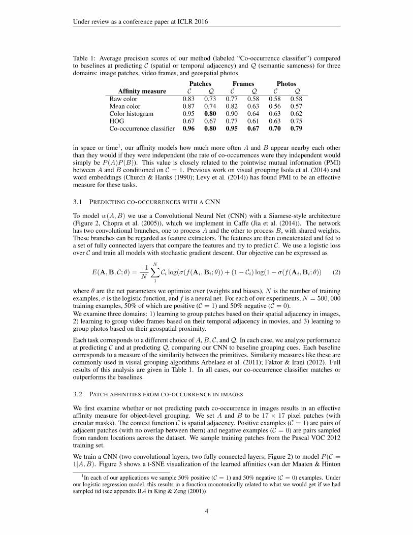
Table 1: Average precision scores of our method (labeled “Co-occurrence classifier”) comparedto baselines at predicting C (spatial or temporal adjacency) and Q (semantic sameness) for threedomains: image patches, video frames, and geospatial photos.

Patches Frames PhotosAffinity measure C Q C Q C Q

Raw color 0.83 0.73 0.77 0.58 0.58 0.58Mean color 0.87 0.74 0.82 0.63 0.56 0.57Color histogram 0.95 0.80 0.90 0.64 0.63 0.62HOG 0.67 0.67 0.77 0.61 0.63 0.75Co-occurrence classifier 0.96 0.80 0.95 0.67 0.70 0.79

in space or time1, our affinity models how much more often A and B appear nearby each otherthan they would if they were independent (the rate of co-occurrences were they independent wouldsimply be P (A)P (B)). This value is closely related to the pointwise mutual information (PMI)between A and B conditioned on C = 1. Previous work on visual grouping Isola et al. (2014) andword embeddings (Church & Hanks (1990); Levy et al. (2014)) has found PMI to be an effectivemeasure for these tasks.

3.1 PREDICTING CO-OCCURRENCES WITH A CNN

To model w(A,B) we use a Convolutional Neural Net (CNN) with a Siamese-style architecture(Figure 2, Chopra et al. (2005)), which we implement in Caffe (Jia et al. (2014)). The networkhas two convolutional branches, one to process A and the other to process B, with shared weights.These branches can be regarded as feature extractors. The features are then concatenated and fed toa set of fully connected layers that compare the features and try to predict C. We use a logistic lossover C and train all models with stochastic gradient descent. Our objective can be expressed as

E(A,B, C; θ) = −1N

N∑1

Ci log(σ(f(Ai,Bi; θ)) + (1− Ci) log(1− σ(f(Ai,Bi; θ)) (2)

where θ are the net parameters we optimize over (weights and biases), N is the number of trainingexamples, σ is the logistic function, and f is a neural net. For each of our experiments,N = 500, 000training examples, 50% of which are positive (C = 1) and 50% negative (C = 0).We examine three domains: 1) learning to group patches based on their spatial adjacency in images,2) learning to group video frames based on their temporal adjacency in movies, and 3) learning togroup photos based on their geospatial proximity.

Each task corresponds to a different choice ofA,B, C, andQ. In each case, we analyze performanceat predicting C and at predicting Q, comparing our CNN to baseline grouping cues. Each baselinecorresponds to a measure of the similarity between the primitives. Similarity measures like these arecommonly used in visual grouping algorithms Arbelaez et al. (2011); Faktor & Irani (2012). Fullresults of this analysis are given in Table 1. In all cases, our co-occurrence classifier matches oroutperforms the baselines.

3.2 PATCH AFFINITIES FROM CO-OCCURRENCE IN IMAGES

We first examine whether or not predicting patch co-occurrence in images results in an effectiveaffinity measure for object-level grouping. We set A and B to be 17 × 17 pixel patches (withcircular masks). The context function C is spatial adjacency. Positive examples (C = 1) are pairs ofadjacent patches (with no overlap between them) and negative examples (C = 0) are pairs sampledfrom random locations across the dataset. We sample training patches from the Pascal VOC 2012training set.

We train a CNN (two convolutional layers, two fully connected layers; Figure 2) to model P (C =1|A,B). Figure 3 shows a t-SNE visualization of the learned affinities (van der Maaten & Hinton

1In each of our applications we sample 50% positive (C = 1) and 50% negative (C = 0) examples. Underour logistic regression model, this results in a function monotonically related to what we would get if we hadsampled iid (see appendix B.4 in King & Zeng (2001))

4

Under review as a conference paper at ICLR 2016

Figure 3: t-SNE visualizations of the learned affinities in each domain. We construct an affinitymatrix between 3000 randomly sampled primitives to create each visualization, using w(A,B) asthe affinity measure. We then apply t-SNE on this matrix (van der Maaten & Hinton (2009)). Toavoid clutter, we visualize the embedded primitives snapped to the nearest point on a grid. Thelearned affinities pick up on different kinds of similarity in each domain. Patches are arrangedlargely according to color, while the geo-photo affinities are less dependent on color, as can be seenin the inset where day and night waterfronts map to nearby points in the t-SNE embedding.

(2009)). As can be seen, the network learns to associate patches with different kinds of structuresuch as texture, local features, and color similarities.

To evaluate performance, we sample 10,000 patches from the Pascal VOC 2012 validation set, 50%with C = 1 and 50% with C = 0. In Table 1 we measure the Average Precision of using severalaffinity measures as a binary classifier of either C or Q. In this case, we defined Q to indicatewhether or not the center pixel of the two patches lies on the same labeled object instance. To testQindependently from C we create theQ test set by only sampling from patch pairs for which C = 1 (sothe net cannot do well at predictingQ simply by doing well at predicting C). Our network performswell relative to the baseline affinity metrics, although color histogram similarity does reach a similarperformance on predicting Q.

Even though it was only trained to predict C, our method is effective at predictingQ as well, achiev-ing an average precision (AP) of 0.80. This validates that spatial proximity, C, is a good surrogatefor “same object”, Q. This raises the question, would we do any better if we directly trained on Q?We tested this, training a new network on 50% patches with Q = 1 and 50% with Q = 0. Thisnet achieves higher performance on predicting Q (AP = 0.85) and lower performance at predictingC (AP = 0.92), than our net trained to predict C. Therefore, although predicting co-occurrence maybe a decent proxy for predicting semantic sameness, there is still a gap in performance compared todirectly training on Q. Designing better context functions, C, that narrow this gap is an importantdirection for future research.

3.3 FRAME AFFINITIES FROM CO-OCCURRENCE IN MOVIES

Our framework can also be applied to learning temporal associations. To test this, we set A and Bto be frames, cropped and down sampled to 33 × 33 pixels, from a set of 96 movies sampled fromthe top 100 rated movies on IMDB2. In this setting, C indicates temporal adjacency – specifically,

2http://www.imdb.com/

5

Under review as a conference paper at ICLR 2016

Table 2: Probing the learned affinities by transforming B while leaving A unmodified. Each num-ber reports the mean output, w(A,B), from each network after the specified transformation hasbeen applied. Transformations applied to one example patch are shown at the top of each column.Comparison should be made with respect to the unmodified input, given in the left-most column.

Vertical Horizontal Color LuminanceNo transformation Rotated 90◦ mirror mirror removed darkened

Patches 0.819 0.818 0.818 0.819 0.382 0.523Frames 0.817 0.794 0.772 0.813 0.264 0.608Photos 0.550 0.488 0.499 0.546 0.520 0.516

two frames are assigned C = 1 if they are at least 3 seconds from each other and not more than 10seconds apart. C = 0 otherwise.

Again we train a CNN to model P (C = 1|A,B) (three convolutional layers, two fully connectedlayers). To evaluate predicting C, we train on half the movies and test on the remaining half. Ourmethod can learn to predict C quite effectively, reaching an Average Precision of 0.95 on the test set.

How do the learned temporal associations relate to semantic visual scenes? To test this, we comparedagainst DVD chapter annotations, setting Q to be “do these two frames occur in the same DVDchapter?” We sample 10,000 frame pairs, 50% with Q = 1 and 50% with Q = 0, while holdingC constant (so that good performance at predicting Q cannot be achieved simply by doing well atpredicting C). Our network achieves an AP of 0.67 on this task. Similar to above, we can then seethat temporal adjacency, C, is an effective surrogate for learning about semantic sameness, Q.

3.4 PHOTO AFFINITIES FROM GEOSPATIAL CO-OCCURRENCE

Just as an object is a collection of associated patches, and a movie scene is a collection of associatedframes, a visual place can be viewed a collection of associated photographs. Here we set A and Bto be geotagged photos, cropped and down sampled to 33 × 33 pixels, and C indicates whether ornot A and B are taken within 11 meters of one another (we exclude exact duplicate locations).

Using the same CNN architecture as for the movie frame network, we again learn P (C = 1|A,B),but for this new setting of the variables. We train on five cities selected from the MIT City DatabaseZhou et al. (2014) and test predicting C on a held out set of three more cities from that dataset. Wealso test how well the network predicts place semantics. For this, we define Q as “do these twophotos belong to the same place category?” We test this task on the LabelMe Outdoors dataset Liuet al. (2009) for which each photo was assigned to one of eight place categories (e.g., “coast”, “high-way”, “tall building”). Our network shows promising performance on this task, reaching 0.79 APon predicting Q. HOG similarity reaches the same performance, which corroborates past findingsthat HOG is effective at grouping related photos (Dalal & Triggs (2005)).

Notice that while HOG does well on associating photographs, it does not do well at associatingmovie frames nor image patches. On the other hand, color histogram similarity does well on associ-ating image patches and movie frames, but fails at grouping everyday photographs – while patcheson an object, or frames in a movie scene, may tend to all use a consistent color palette, tourist photosof the same location will have high color variance, due to seasonal and lighting variations. Differentgrouping rules will be effective at different tasks. Our learning based approach has the advantagethat it automatically figures out the appropriate grouping cue for each new domain, and therebyachieves good performance on all our tasks.

3.5 WHICH CUES DID THE NETWORKS LEARN TO USE?

In each domain tested above, the grouping rules may be very different. Here we study them byprobing the trained networks with controlled stimuli. Similar to how a psychophysicist might exper-iment on human perception, we show our networks specially made stimuli. For each test, we feedthe networks many pairs {A,B}, sampled from locations such that C = 1. We leaveA unaltered, butmodify B in a controlled way. This allows us to test what kinds of transformations of B will change

6

Under review as a conference paper at ICLR 2016

ABO: 0.79, recall: 1.00ABO: 0.79, recall: 1.00ABO: 0.79, recall: 1.00ABO: 0.79, recall: 1.00ABO: 0.79, recall: 1.00ABO: 0.88, recall: 1.00ABO: 0.88, recall: 1.00ABO: 0.88, recall: 1.00ABO: 0.88, recall: 1.00ABO: 0.88, recall: 1.00

ABO: 0.44, recall: 0.00ABO: 0.44, recall: 0.00ABO: 0.44, recall: 0.00ABO: 0.44, recall: 0.00ABO: 0.44, recall: 0.00

ABO: 0.69, recall: 1.00ABO: 0.69, recall: 1.00ABO: 0.69, recall: 1.00ABO: 0.69, recall: 1.00ABO: 0.69, recall: 1.00ABO: 0.66, recall: 1.00ABO: 0.66, recall: 1.00ABO: 0.66, recall: 1.00ABO: 0.66, recall: 1.00ABO: 0.66, recall: 1.00

ABO: 0.68, recall: 1.00ABO: 0.68, recall: 1.00ABO: 0.68, recall: 1.00ABO: 0.68, recall: 1.00ABO: 0.68, recall: 1.00

ABO: 0.67, recall: 1.00ABO: 0.67, recall: 1.00ABO: 0.67, recall: 1.00ABO: 0.67, recall: 1.00ABO: 0.67, recall: 1.00 ABO: 0.65, recall: 1.00ABO: 0.65, recall: 1.00ABO: 0.65, recall: 1.00ABO: 0.65, recall: 1.00ABO: 0.65, recall: 1.00 ABO: 0.74, recall: 1.00ABO: 0.74, recall: 1.00ABO: 0.74, recall: 1.00ABO: 0.74, recall: 1.00ABO: 0.74, recall: 1.00

ABO: 0.40, recall: 0.00ABO: 0.40, recall: 0.00ABO: 0.40, recall: 0.00ABO: 0.40, recall: 0.00ABO: 0.40, recall: 0.00 ABO: 0.16, recall: 0.10ABO: 0.16, recall: 0.10ABO: 0.16, recall: 0.10ABO: 0.16, recall: 0.10ABO: 0.16, recall: 0.10 ABO: 0.36, recall: 0.44ABO: 0.36, recall: 0.44ABO: 0.36, recall: 0.44ABO: 0.36, recall: 0.44ABO: 0.36, recall: 0.44

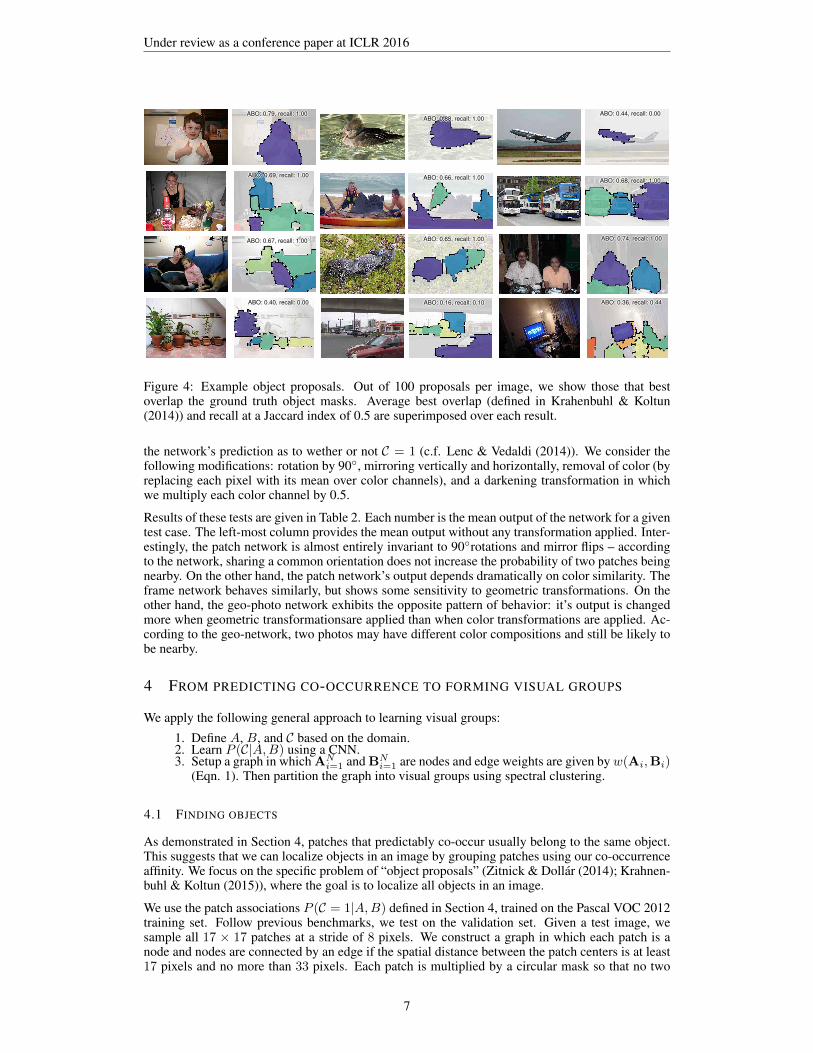
Figure 4: Example object proposals. Out of 100 proposals per image, we show those that bestoverlap the ground truth object masks. Average best overlap (defined in Krahenbuhl & Koltun(2014)) and recall at a Jaccard index of 0.5 are superimposed over each result.

the network’s prediction as to wether or not C = 1 (c.f. Lenc & Vedaldi (2014)). We consider thefollowing modifications: rotation by 90◦, mirroring vertically and horizontally, removal of color (byreplacing each pixel with its mean over color channels), and a darkening transformation in whichwe multiply each color channel by 0.5.

Results of these tests are given in Table 2. Each number is the mean output of the network for a giventest case. The left-most column provides the mean output without any transformation applied. Inter-estingly, the patch network is almost entirely invariant to 90◦rotations and mirror flips – accordingto the network, sharing a common orientation does not increase the probability of two patches beingnearby. On the other hand, the patch network’s output depends dramatically on color similarity. Theframe network behaves similarly, but shows some sensitivity to geometric transformations. On theother hand, the geo-photo network exhibits the opposite pattern of behavior: it’s output is changedmore when geometric transformationsare applied than when color transformations are applied. Ac-cording to the geo-network, two photos may have different color compositions and still be likely tobe nearby.

4 FROM PREDICTING CO-OCCURRENCE TO FORMING VISUAL GROUPS

We apply the following general approach to learning visual groups:

1. Define A, B, and C based on the domain.2. Learn P (C|A,B) using a CNN.3. Setup a graph in which AN

i=1 and BNi=1 are nodes and edge weights are given byw(Ai,Bi)

(Eqn. 1). Then partition the graph into visual groups using spectral clustering.

4.1 FINDING OBJECTS

As demonstrated in Section 4, patches that predictably co-occur usually belong to the same object.This suggests that we can localize objects in an image by grouping patches using our co-occurrenceaffinity. We focus on the specific problem of “object proposals” (Zitnick & Dollar (2014); Krahnen-buhl & Koltun (2015)), where the goal is to localize all objects in an image.

We use the patch associations P (C = 1|A,B) defined in Section 4, trained on the Pascal VOC 2012training set. Follow previous benchmarks, we test on the validation set. Given a test image, wesample all 17 × 17 patches at a stride of 8 pixels. We construct a graph in which each patch is anode and nodes are connected by an edge if the spatial distance between the patch centers is at least17 pixels and no more than 33 pixels. Each patch is multiplied by a circular mask so that no two

7

Under review as a conference paper at ICLR 2016

100 101 102

# of boxes

0.2

0.4

0.6

0.8

Aver

age

Best

Ove

rlap

BINGEdge BoxesGOPLPOObjectnessCo-occurenceRandomized PrimSel. Search

100 101 102

# of boxes

0.0

0.2

0.4

0.6

Aver

age

Reca

ll

0.5 0.6 0.7 0.8 0.9 1.0J

0.0

0.2

0.4

0.6

0.8

Reca

ll

50 proposals

Figure 5: Object proposal results, evaluated on bounding boxes. Our unsupervised method (labeled“Co-occurrence”) is competitive with recent supervised algorithms at proposing up to around 100objects. ABO is the average best overlap metric from (Krahenbuhl & Koltun (2014)), J is Jaccardindex. The papers compared to are: BING (Cheng et al. (2014)), EdgeBoxes Zitnick & Dollar(2014), LPO (Krahnenbuhl & Koltun (2015)), Objectness (Alexe et al. (2012)), GOP (Krahenbuhl& Koltun (2014)), Randomized Prim (Manen et al. (2013)), Sel. Search (Uijlings et al. (2013)).

The F

ound

ations

of S

tone

The T

aming

of S

mea

gol

The U

ruk-

hai

The T

hree

Hun

ters

The B

urning

of W

estfo

ld

The B

anishm

ent o

f Eom

er

On

the

Trail of

the

Uru

k-ha

i

Night

Cam

p at

Fan

gorn

The R

ider

s of

Roh

an

DV

D c

hapte

rsD

iscovere

d s

cenes

Recall0 0.1 0.2 0.3 0.4 0.5 0.6 0.7

Pre

cis

ion

0

0.05

0.1

0.15

0.2

0.25

0.3

0.35

0.4

0.45

0.5Movie Scene Boundary Detection

Raw color similarityMean color similarityColor histogram similarityHOG similarityCo-occurrence classifier

Figure 6: Movie scene segmentation results. On the left, we show a “movie barcode” for TheTwo Towers, in which each frame of the movie is resized into a signal column of the visualization;the top shows the DVD chapters and the bottom our recovered scene segmentation. Notice thatsome DVD chapters contain multiple different scenes. Our method tends to detect these sub-chapterscenes, resulting in an over-segmentation compared to the chapters. On the right, we quantify ourperformance on this scene segmentation task; see text for details.

patches connected by an edge see any overlapping pixels (see Figure 2(right)). Each edge, indexedby i, j, is weighted by Wi,j = w(Ai,Bi)

α, resulting in the affinity matrix W, where we use thevalue α = 20 in our experiments.

To globalize the associations, we apply spectral clustering to the matrix W. First we create theLaplacian eigenmap L for W, using the 2nd through 16th eigenvectors with largest eigenvalues.Each eigenvector is scaled by λ−

12 where λ is the corresponding eigenvalue. We then generate

object proposals simply by applying k-means to the Laplacian eigenmap. To generate more than afew proposals, we run k-means multiple times with random restarts and for values of k from 5 to16. Finally, we prune redundant proposals and sort proposals to achieve diversity throughout theranking (by encouraging proposals to be made from different values of k before giving proposalsfrom a random restart at the same value of k).

Qualitative results from our method are shown in Figure 4. In each case, we show the proposals thathave best overlap with the ground truth object masks for 100 proposals. We quantitatively compareagainst other recent methods in Figure 5. Even though our method is not trained on labeled images,it reaches performance comparable to recent supervised methods at proposing up to 100 objects perimage. Our implementation runs in about 4 seconds per image on a 2015 Macbook Pro.

4.2 SEGMENTING MOVIESJust as objects are composed of associated patches, scenes in a movie are composed of associatedframes. Here we show how our learned frame affinities can be used to break a movie into coherentscenes, a problem that has received some prior attention (Chen et al. (2008); Zhai & Shah (2006)).

8

Under review as a conference paper at ICLR 2016

k0 2 4 6 8 10 12 14 16

pu

rity

0.1

0.2

0.3

0.4

0.5

0.6

0.7Photo clustering purity

Raw color similarityMean color similarityColor histogram similarityHOG similarityCo-occurrence classifier

Figure 7: Left: Clustering the LabelMe Outdoor dataset (Liu et al. (2009)) into 8 groups using ourlearned affinities. Random sample images are shown from each group. Right: Photo cluster purityversus number of clusters k. Note that we trained our model on an independent dataset, the MITCity dataset (Zhou et al. (2014)).

To segment a movie, we build a graph in which each frame is a node and all frames within tenseconds of one another are connected by an edge. We then weight the edges using the frame-associations P (C = 1|A,B) (Section 4), and partition the graph using spectral clustering.

To evaluate, we use DVD chapter annotations as ground truth. Following a standard evaluationprocedure in image boundary detection (Arbelaez et al. (2011)), we measure performance on theretrieval task of finding all ground truth boundaries. In Figure 6(right), we compare against thebaseline affinity metrics from Section 4. In each case, we apply the same spectral clustering pipelineas for our method, except with edge weights given by the baseline metrics instead of by our net. Itis important to properly scale each similarity metric or else spectral clustering will fail. To providefair comparison, we sweep over a range of scale factors α, setting edge weights as exp(w(A,B)

α2 ),where w is the affinity measure. In Figure 6(right) we show results selecting the optimal α for eachmethod.

Our approach finds more boundaries with higher precision than these baselines, except for colorhistogram similarity, which reaches a similar performance. Figure 6 (left) shows an example seg-mentation of a section of The Two Towers. The movie is displayed as a “movie barcode”3 in whicheach frame is squished into a single column and time advances to the right. On top are the DVDchapter annotations, and on the bottom are our inferred boundaries.

4.3 DISCOVERING PLACE CATEGORIES

Taking the geospatial-associations model from Section 4, we cluster photos into coherent types ofplaces. Here we create a fully connected graph between all photos in a given collection, weight theedges with P (C = 1|A,B) and then apply spectral clustering to partition the collection. We testthe purity of the clusters on LabelMe Outdoors dataset (Liu et al. (2009)). Clustering purity versusnumber of clusters k is given in Figure 7 (right), showing that our method is effective at discoveringsemantic place categories. As in our movie segmentation experiments, we select the optimal α toscale the affinity of our method as well each baseline. Figure 7 (left) shows random sample imagesfrom each cluster after clustering into 8 categories. This clustering has 59% purity.

5 CONCLUSION

We have presented a simple and general approach to learning visual groupings, which requires nopre-defined labels. Instead our framework uses co-occurrence in space or time as a supervisorysignal. By doing so, we learn different clustering mechanisms for a variety of tasks. Our approachachieves competitive results on object proposal generation, even when compared to methods trainedon labeled data. Additionally, we demonstrated that the same method can be used to segment moviesinto scenes and to uncover semantic place categories. The principles underlying the framework arequite general and may be applicable to data in other domains, when there are natural co-occurrencesignals and groupings.

3http://moviebarcode.tumblr.com/

9

Under review as a conference paper at ICLR 2016

ACKNOWLEDGMENTS

We thank William T. Freeman, Joshua B. Tenenbaum, and Alexei A. Efros for helpful feedback anddiscussions. Thanks to Andrew Owens for helping collect the movie dataset. This work is supportedby NSF award 1161731, Understanding Translucency, and by Shell Research.

REFERENCES

Agrawal, Pulkit, Carreira, Joao, and Malik, Jitendra. Learning to see by moving. arXiv preprintarXiv:1505.01596, 2015.

Alexe, Bogdan, Deselaers, Thomas, and Ferrari, Vittorio. Measuring the objectness of image windows. PAMI,2012.

Arbelaez, Pablo, Maire, Michael, Fowlkes, Charless, and Malik, Jitendra. Contour detection and hierarchicalimage segmentation. PAMI, 33(5):898–916, 2011.

Barlow, Horace. Cerebral cortex as model builder. Models of the visual cortex, pp. 37–46, 1985.

Canny, John. A computational approach to edge detection. PAMI, (6):679–698, 1986.

Chen, Liang-Hua, Lai, Yu-Chun, and Liao, Hong-Yuan Mark. Movie scene segmentation using backgroundinformation. Pattern Recognition, 41(3):1056–1065, 2008.

Cheng, Ming-Ming, Zhang, Ziming, Lin, Wen-Yan, and Torr, Philip. Bing: Binarized normed gradients forobjectness estimation at 300fps. In CVPR, 2014.

Chopra, Sumit, Hadsell, Raia, and LeCun, Yann. Learning a similarity metric discriminatively, with applicationto face verification. In Computer Vision and Pattern Recognition, 2005. CVPR 2005. IEEE Computer SocietyConference on, volume 1, pp. 539–546. IEEE, 2005.

Church, Kenneth Ward and Hanks, Patrick. Word association norms, mutual information, and lexicography.Computational linguistics, 16(1):22–29, 1990.

Dalal, Navneet and Triggs, Bill. Histograms of oriented gradients for human detection. In CVPR, 2005.

Doersch, Carl, Gupta, Abhinav, and Efros, Alexei A. Unsupervised visual representation learning by contextprediction. CoRR, abs/1505.05192, 2015. URL http://arxiv.org/abs/1505.05192.

Dollar, Piotr and Zitnick, C Lawrence. Structured forests for fast edge detection. In ICCV, 2013.

Faktor, Alon and Irani, Michal. Clustering by composition–unsupervised discovery of image categories. InECCV. 2012.

Faktor, Alon and Irani, Michal. Co-segmentation by composition. In ICCV, 2013.

Fiser, Jozsef and Aslin, Richard N. Unsupervised statistical learning of higher-order spatial structures fromvisual scenes. Psychological science, 12(6):499–504, 2001.

Isola, Phillip, Zoran, Daniel, Krishnan, Dilip, and Adelson, Edward H. Crisp boundary detection using point-wise mutual information. In ECCV, 2014.

Jayaraman, Dinesh and Grauman, Kristen. Learning image representations equivariant to ego-motion. arXivpreprint arXiv:1505.02206, 2015.

Jia, Yangqing, Shelhamer, Evan, Donahue, Jeff, Karayev, Sergey, Long, Jonathan, Girshick, Ross, Guadarrama,Sergio, and Darrell, Trevor. Caffe: Convolutional architecture for fast feature embedding. In Proceedings ofthe ACM International Conference on Multimedia, pp. 675–678. ACM, 2014.

Kayser, Christoph, Einhauser, Wolfgang, Dummer, Olaf, Konig, Peter, and Kording, Konrad. Extracting slowsubspaces from natural videos leads to complex cells. In Artificial Neural Networks?ICANN 2001, pp.1075–1080. Springer, 2001.

King, Gary and Zeng, Langche. Logistic regression in rare events data. Political analysis, 9(2):137–163, 2001.

Krahenbuhl, Philipp and Koltun, Vladlen. Geodesic object proposals. In ECCV. 2014.

Krahnenbuhl, Phillip and Koltun, Vladlen. Learning to propose objects. In CVPR, 2015.

10

Under review as a conference paper at ICLR 2016

Lenc, Karel and Vedaldi, Andrea. Understanding image representations by measuring their equivariance andequivalence. arXiv preprint arXiv:1411.5908, 2014.

Levy, Omer, Goldberg, Yoav, and Ramat-Gan, Israel. Linguistic regularities in sparse and explicit word repre-sentations. CoNLL-2014, pp. 171, 2014.

Liu, Ce, Yuen, Jenny, and Torralba, Antonio. Nonparametric scene parsing: Label transfer via dense scenealignment. In CVPR, 2009.

Lowe, David. Perceptual organization and visual recognition, volume 5. Springer Science & Business Media,2012.

Malisiewicz, Tomasz and Efros, Alexei A. Improving spatial support for objects via multiple segmentations.In BMVC, 2007.

Manen, Santiago, Guillaumin, Matthieu, and Gool, Luc Van. Prime object proposals with randomized prim’salgorithm. In ICCV, 2013.

Mobahi, Hossein, Collobert, Ronan, and Weston, Jason. Deep learning from temporal coherence in video. InBottou, Leon and Littman, Michael (eds.), ICML, pp. 737–744, Montreal, June 2009. Omnipress.

Rock, Irvin. The logic of perception. 1983.

Saffran, Jenny R, Aslin, Richard N, and Newport, Elissa L. Statistical learning by 8-month-old infants. Science,274(5294):1926–1928, 1996.

Schapiro, Anna C, Rogers, Timothy T, Cordova, Natalia I, Turk-Browne, Nicholas B, and Botvinick,Matthew M. Neural representations of events arise from temporal community structure. Nature Neuro-science, 16(4):486–492, 2013.

Shi, Jianbo and Malik, Jitendra. Normalized cuts and image segmentation. PAMI, 22(8):888–905, 2000.

Sivic, Josef, Russell, Bryan C, Efros, Alexei, Zisserman, Andrew, Freeman, William T, et al. Discoveringobjects and their location in images. In Computer Vision, 2005. ICCV 2005. Tenth IEEE InternationalConference on, volume 1, pp. 370–377. IEEE, 2005.

Srivastava, Nitish, Mansimov, Elman, and Salakhutdinov, Ruslan. Unsupervised learning of video representa-tions using lstms. arXiv preprint arXiv:1502.04681, 2015.

Tenenbaum, Jay M and Witkin, AP. On the role of structure in vision. Human and machine vision, pp. 481–543,1983.

Uijlings, Jasper RR, van de Sande, Koen EA, Gevers, Theo, and Smeulders, Arnold WM. Selective search forobject recognition. IJCV, 104(2):154–171, 2013.

van der Maaten, L.J.P. and Hinton, G.E. Visualizing high-dimensional data using t-sne. Journal of MachineLearning Research, 2009.

Wang, Xiaolong and Gupta, Abhinav. Unsupervised learning of visual representations using videos. arXivpreprint arXiv:1505.00687, 2015.

Wilkin, Andrew P and Tenenbaum, Jay M. What is perceptual organization for? From Pixels to Predicates,1985.

Wiskott, Laurenz and Sejnowski, Terrence J. Slow feature analysis: Unsupervised learning of invariances.Neural computation, 14(4):715–770, 2002.

Zhai, Yun and Shah, Mubarak. Video scene segmentation using markov chain monte carlo. Multimedia, IEEETransactions on, 8(4):686–697, 2006.

Zhou, B., Liu, Liu., Oliva, A., and Torralba, A. Recognizing City Identity via Attribute Analysis of Geo-taggedImages. ECCV, 2014.

Zitnick, C Lawrence and Dollar, Piotr. Edge boxes: Locating object proposals from edges. In ECCV. 2014.

11