Dagmawi Mallie

VOICE PROCESSING USING MATLAB

AS A TOOL

Technology and Communication

2014

Acknowledgements

I would like to express my sincerest gratitude and appreciation to my supervisor,

Dr. Gao Chao, for his assistance throughout the process of the project, but more

importantly, for attracting my attention to this subject in the first place. Without

saying, Dr. Gao Chao had patently guided me throughout the process of this thesis

project. Through carrying out the research required for this thesis, I have cemented

the interest in speech processing.

I now hope to continue studying towards higher degree in Digital Signal Processing,

and it is largely due to the experience that I have had through researching for this

thesis.

I would also like to thank all the instructors I have the privilege of being their

student. I am also utmost grateful to my family and friends for the support and

encouragement I received over the years.

iii

VAASAN AMMATTIKORKEAKOULU

UNIVERSITY OF APPLIED SCIENCES

Information Technology

ABSTRACT

Author Dagmawi Mallie

Title Voice Processing Using MATLAB as a Tool

Year 2014

Language English

Pages 45 + 8

Name of Supervisor Gao Chao

The objective of this thesis was to apply phase vocoder, reverberator along with

some basic signal filters to a speech signal that is either recorded or stored in the

folder. These speech processing algorithms are arranged in the cascading manner

so that the user has an option either to choose or ignore the algorithms to bring

any effect on the input sound signal.

The algorithms of these speech coding techniques were demonstrated and

obtained with the aid of MATLAB. For better understanding the output and input

of signals can be plotted on separate figures. It also provides the three most

common ways of plotting signals which are time domain, frequency domain, and

spectrogram.

CONTENTS

ABSTRACT

1 INTRODUCTION ............................................................................................ 8

1.1 General Introduction ................................................................................. 8

1.2 Motivation ................................................................................................. 8

1.3 Aim of Thesis ............................................................................................ 8

1.4 Overview of the Project ............................................................................ 9

1.5 Overview of the Thesis ........................................................................... 10

2 THEORETICAL BACKGROUND OF THE PROJECT............................... 12

2.1 Background ............................................................................................. 12

2.2 Filters ...................................................................................................... 12

2.2.1 Background of Filters .................................................................... 12

2.2.2 Filter Design .................................................................................. 12

2.2.3 Filter Classification ....................................................................... 13

2.2.4 Filter Requirement and Specifications .......................................... 13

2.2.5 Filter Implementations................................................................... 14

2.3 Pitch Shifting .......................................................................................... 15

2.3.1 Background.................................................................................... 15

2.3.2 Mathematics Behind the Algorithm .............................................. 15

2.3.3 Phase Vocoder ............................................................................... 18

2.4 Reverberation .......................................................................................... 21

2.4.1 Background.................................................................................... 21

2.4.2 Approaches to Reverberation Algorithm ....................................... 22

2.4.3 Early Reverberation ....................................................................... 23

2.4.4 Schroeder’s Reverberator .............................................................. 24

3 MATLAB GUI ............................................................................................... 28

3.1 Background ............................................................................................. 28

3.2 Programming GUI Application in MATLAB......................................... 28

3.3 How to Build MATLAB GUI ................................................................. 29

3.4 Comparing the Two Versions of Voice Processing Tool ....................... 29

3.5 The GUI’s Task....................................................................................... 30

5

3.6 Looking In depth Each Sections of the GUI ........................................... 33

3.6.1 Data Center Section ....................................................................... 33

3.6.1.1 Load Push Button ............................................................ 33

3.6.1.2 Record Push Button ......................................................... 34

3.6.1.3 Play and Save Original Sound Buttons ........................... 35

3.7 Filter Components ................................................................................... 37

3.8 Sound Processing Section ....................................................................... 40

3.8.1 Pitch Shift Slider............................................................................ 40

3.8.2 Reverb and Volume Radio Buttons ............................................... 42

3.8.3 Process Pushbutton ........................................................................ 42

3.9 Graph Section.......................................................................................... 44

4 CONCLUSION .............................................................................................. 49

5 REFERENCES ............................................................................................... 51

LIST OF FIGURES

Figure 1. GUI of the project 10

Figure 2. Schematic diagram of Schroeder reverberator 24

Figure 3. Comb filter 25

Figure 4. All-Pass filter 27

Figure 5. The activation hierarchy 33

Figure 6. The Data section of the GUI 33

Figure 7. Flow chart for the buttons of Data Section 37

Figure 8. The Filter section 38

Figure 9. Flow chart for filter section radio buttons 39

Figure 10. The sound processing section of the GUI 40

Figure 11. Flow chart for pitch_slider_Callback function 41

Figure 12. Flow chart for process pushbutton 44

Figure 13. The Graph section 45

Figure 14. Sound signal in time domain 46

Figure 15. Frequency spectrum of the sound signal 47

Figure 16. Spectrogram of the sound signal 48

7

LIST OF ABBREVIATION

BPF: Band Pass Filter, 13

BSF: Band Stop Filter, 13

DFT: Discrete Fourier Transform, 16

FDATool: Filter Design and Analysis Tool, 14

FFT: Fast Fourier Transform, 16

FIR: Finite Impulse Response, 12

GUI: Graphical User Interface, 8

GUIDE: Graphical User Interface Development Environment, 30

HPF: High Pass Filter, 13

IFFT: Inverse Fast Fourier Transform, 20

IIR: Infinite Impulse Response, 12

ISTFT: Inverse Short Time Fourier Transform, 18

LPF: Low-pass Filter, 13

MATLAB: Matrix Laboratory, 8

STFT: Short Time Fourier Transform, 17

UI: User Interface, 36

1 INTRODUCTION

1.1 General Introduction

Speech is a form of communication in everyday life. It has existed since human

civilizations began. Speech is applied to high technological telecommunication

systems. Scientists began formulating algorithms which might change the nature of

voice signal since the 1970s after the emergence of digital devices.

The core of signal processing is a way of looking at the signals in terms of sinusoidal

components of various frequencies (the Fourier domain) /15/. The techniques for

categorizing signals in their frequency domain, filtering, developed on analog

electronics but after the 1970s signal processing has more and more been

implemented on computers in the digital domain.

In this thesis, we will be looking more into speech processing with the aid of an

interesting technology known as MATLAB. MATLAB (Matrix Laboratory)

becomes the de facto tool in digital signal processing. MATLAB is a well-known

tool for numerical calculations, this thesis employs its GUI (Graphical User

Interface) features as well. This makes MATLAB a perfect tool for the application

this thesis deals with.

1.2 Motivation

Speech processing is one of the fastest growing subjects. Its applications are also

expanding very fast. The rapid growth of the computational capabilities of digital

machines accelerates its application. During this growth there has been a close

relationship between the development of new algorithms and theoretical results.

New and improved techniques are always coming into play but these days most of

them are protected by proprietary rights and their actual algorithm is hidden from

the mass.

Pitch shifting, reverberation, and filtering sound signal are the most basic types of

speech processing application. Pitch shifting is common in music and movie

industry. Especially electronic musicians apply pitch-shifted samples of vocal

9

melodies. Cartoon films are also another entertainment sector which widely uses

pitch shifter to produce distinctive sounds.

Artificial reverberation also plays a vital role in production of music. As recordings

are made in an acoustically dead studio with close-microphone voices, there is

literally no reverberation of the sound signal. As a result, composers can add this

reverberation artificially to the music.

The motivation of this thesis is by studying these basic types of sound processing

techniques, thereby improving the GUI and processing capabilities of voice

processing tool version 1.

1.3 Aim of Thesis

The primary goal of this thesis was to design a MATLAB based application which

can shift the pitch, add reverberation and filter certain frequencies out of the sound

signal which is either recorded by the application or imported from a saved *.wav

file.

The mentioned modules of the application are arranged in a cascaded fashion that

the final output signal feels the work of each function. To compare the effect of the

modules on the signal the application is powered with graphs which can be plotted

in three different manners.

1.4 Overview of the Project

This voice processing demo project is capable either recording a voice for 5 seconds

or loading a *.wav file. Once the demo receives the file it provides the option of

playing it or saving it for later use. The modules are also cascaded in the same

manner as they are presented on the GUI. In order to activate the module one needs

to check the check boxes first then their respective text boxes become activated.

The demo understands the input values of the text boxes in the filter section as Hertz

and in the sound processing section as decibel. The pitch shifting slide bar becomes

active after the sound data is loaded to the program. Pressing the process button will

trigger the actions to be performed on the signal based on the values the user fed in.

Figure 1 shows the GUI of the demo project.

Figure 1. GUI of the project

Figure 2. GUI Version I

1.5 Overview of the Thesis

The above serves as a general description on the scope of this thesis. The motivation

behind this research and the aim of this thesis are discussed in this chapter.

11

Chapter 2 is about filters. Filters are the backbone of signal processing, therefore

enough emphasis has been put so as to cover the most fundamental types. The

chapter clarifies the types of filters used in the project starting from their basic

definition and nature. Filter design methodologies and tools MATLAB offers have

also been studied. The design requirements, specification used for their design and

their implementation details has been presented in detail.

Pitch shifting design and implementation follows the filter section. This section of

the chapter describes in detail the pitch shifting starting from the theory to

implementation details. The chapter begins with the production of human voice,

then it goes on to illustrate what pitch means in signal processing subject.

Mathematical details have also been given enough attention together with the

implementation and coding.

The final section of the chapter is the Schroeder’s reverberator. The chapter deals

with enough details of the background theory and the algorithm needed to create a

Schroeder reverberator.

Chapter 3 is about MATLAB GUI. This chapter deals with how MATLAB GUI

technology is adapted and used for the benefit of the project. The

intercommunication among the different GUI components has also been explained

thoroughly. A flow chart is also included in every component description section

so as to make the illustration more visual.

Chapter 4 concludes the thesis by telling something about the gains and challenges

received from the project. Some ideas have also been suggested about possible

future improvements for the future research work.

2 THEORETICAL BACKGROUND OF THE PROJECT

2.1 Background

This voice processing MATLAB project was developed based on three main

algorithms. These algorithms are the basic digital signal processing filtering

techniques, Flanagan’s pitch shifting vocoder and Schroeder reverberation. This

chapter explains how each one of these algorithms was adopted in this project.

2.2 Filters

2.2.1 Background of Filters

Digital filters are implemented so as to eliminate the unwanted frequencies of the

signal components from the signal being processed. A digital filter uses various

functions to compute the input signal. These filters are composed of distinct pattern

of multiplications and additions. Adders, multipliers and delay units are considered

as the building blocks of filters.

MATLAB offers a number of ways to implement filters. Each function takes a

number of different input arguments along with the sound signal and returns the

processed signal. In the filters section of this project, there are four different filter

functions. They are low pass filter, high pass filter, band pass filter, and band stop

filter.

2.2.2 Filter Design

We can classify filters in several different groups but the major types are, FIR

(Finite Impulse Response) and IIR (Infinite Impulse Response) filters.

Both types of filters offer some advantages and there are also disadvantages that

need to be carefully studied during designing. As an example, a speech signal can

be processed in systems with non-linear phase characteristic. The phase

characteristic of a speech signal is not of the essence and as such can be

neglected/12/, which results in the possibility to use a much wider range of systems

for its processing. Whereas signals obtained from various sensors in industry have

to be in a linear phase so as to prevent losing vital information /12/.

13

FIR filters have been used in this demo project. The FIR filters are easy to implement

but a large impulse response duration is required to adequately approximate the cutoff

frequency.

There are three well-known methods to design a FIR filter. These three methods

are:

- Window design

- Frequency Sampling Design

- Optimal Design

The Window design is the method used in designing the filters for the Filter section

of the GUI in this thesis.

2.2.3 Filter Classification

The four filter types that were implemented in the filter section of the GUI are the

following.

- A LPF (Low Pass Filter) lets frequencies which are below the cutoff pass

without any distortion while attenuating those above the cutoff.

- A HPF (High Pass Filter) lets signals pass through without any distortion if

they have a higher frequency than the cutoff, otherwise it will attenuate the

signal's amplitude.

- A BPF (Band Pass Filters) are designed to stop the signals with frequencies

below the first cutoff frequency and higher than the second cutoff frequency.

To put it in a different word, it will not distract those signals with frequencies

in between the two cutoff frequencies.

- A BSF (Band Stop Filters) are the exact opposite of band-pass filters as they

are designed to stop the signals with frequencies in between the two cutoff

frequencies.

2.2.4 Filter Requirement and Specifications

Filter design is a process of finding filter coefficients which will give the filter the

competence to meet the specification. MATLAB's Signal Processing Toolbox

offers two methods to realize the filter: the first one is an object-oriented approach

and the other one is a non-object oriented approach /4/.

This project uses the non-object oriented approach for filter design. All of the non-

object oriented filter design modules operate with normalized frequency.

The filter designing function "fir1" has been employed in designing the four types

of filters. Fir1 implements the classical method of windowed linear phase FIR

digital filter design. It resembles the IIR filter design functions in that it is

formulated to design filters in standard band configurations: lowpass, bandpass,

highpass, and bandstop /4/.

Although the Hamming window is not the most efficient windowing technique, it

provides a better performance than the rectangular window, has more or less similar

performance with the Hanning window and it is inferior to the Blackman window

/4/. It is impossible to remove the ripples and ringing which occur especially around

the cutoff frequencies. The implementations of filters in this paper was based on

the hamming window.

2.2.5 Filter Implementations

The implementation of filters in MATLAB was facilitated by the introduction of

FDATool (Filter Design and Analysis Tool) in the signal processing toolkit.

FDATool is a powerful graphical user interface for designing and analyzing filters.

FDATool enables the filter designer to design digital FIR or IIR filters by setting

filter specifications, by importing filters from the MATLAB workspace, or by

adding, moving or deleting poles and zeroes. FDATool also provides tools for

analyzing filters, such as magnitude and phase response and pole-zero plots /4/.

This project designed filters with the help of FDATool window. The FDATool used

the following specification to design the filter.

- Design Method: - FIR Window

- Filter Order: - 100 (Type I filter)

- Window type: - Hamming

- Structure: - Direct form I

15

Listing 1. (lowpass.m) FIR design of low-pass filter

function LOW_PASS = lowpass(Fs,Fc,sound_signal) %LOWPASS Returns a discrete-time filter object.

% % MATLAB Code % Generated by MATLAB(R) 8.0 and the Signal Processing Toolbox 6.18. % %

% FIR Window Lowpass filter designed using the FIR1 function.

% All frequency values are in Hz. N = 100; % Order flag = 'scale'; % Sampling Flag

% Create the window vector for the design algorithm. win = hamming(N+1);

% Calculate the coefficients using the FIR1 function. b = fir1(N, Fc/(Fs/2), 'low', win, flag); Hd = dfilt.dffir(b); LOW_PASS = Hd.filter(sound_signal);

% [EOF]

2.3 Pitch Shifting

2.3.1 Background

Pitch shifting is a sound processing technique in which the original pitch of a sound

is raised or lowered /13/. The pitch is the fundamental frequency of the generated

sound by the vocal cord. When the pitch of a vocal signal is shifted, the formants

of the sound will also be adjusted, whereby changes will come to the character of

the sound.

Pitch shifting algorithms offer the method to keep the formants of the voice signal

as it is, but changing only the pitch. This chapter describes the phase vocoder

algorithm and the various mathematical analyses required for the implementation

of the algorithm.

2.3.2 Mathematics Behind the Algorithm

The Fourier transform is an indispensable tool in the signal analysis. It breaks down

sound signals as a prism splits the white light into its constituents. The Fourier

transform breaks down a complex sound signal into ordinary sine waves which have

their own frequency, amplitude and phase.

When it comes to digital data, the Fourier transform is inapplicable, as it can only

be applied on analogue signals. Whereas DFT (Discrete Fourier Transform) is

another form of Fourier Transform, which can be applied on digital signals. Though

DFT is similar to continuous Fourier Transform, it differs in three useful ways.

First, it applies to discrete-time sequences. Second, it is a sum rather than an

integral. Third, it operates on finite data records. Formula 1 shows the DFT function

/8/.

𝑋(𝑛) = ∑ 𝑥[𝑘] ∗ 𝑒−𝑗2𝜋𝑛𝑘/𝑁𝑁−1𝑘= 0 Where n = 0, 1, 2…N (1) /8/

DFT requires time and resource intensive calculations. Mathematicians proposed

different algorithms which can reduce the steps direct DFT calculation needs. FFT

(Fast Fourier Transform) is one of those algorithms which increase the efficiency

of DFT calculations considerably. MATLAB offers the FFT mechanism which is

built based on the Cooley-Turkey algorithm /4/. This MATLAB function was used

to come up with the Fourier transform of the signal.

When the signal became too long to be analyzed with a single transform STFT

(Short Time Fourier Transform) was used instead. This is a form of analyzing the

entire speech signal by dividing it into smaller chunks of samples. All the analysis,

the phase shifting, and finally the synthesis can be done with these small chunks of

samples with much efficiency and good quality.

STFT performs the FFT algorithm on a selected number of samples at a time. The

process of selecting a fixed number of samples at a time is known as Windowing.

Windowing is the technique which makes all the values outside the window zero

while having different values inside the window. The Hamming window was used

in this thesis.

The length of the window is 256 samples. The number is based on the following

two facts. First, FFT uses 2n number of computations to calculate the Fourier

Transform. Second, the importance of using windowing is to limit the time interval

17

to be analyzed so that the properties of the waveform do not change appreciably.

256 samples with 8000 Hz make the Hamming window 32ms wide. A speech signal

analyzed in the window length of 20 to 30ms would give a good resolution of the

signal /6/.

In STFT, the windows overlap each other. The hop length refers to the length of

the overlapping length between the windows. The hop length used in this project is

1/4th of the window length that would be 64 samples. The summation of the

overlapping parts of the transformed signal is constant.

The following MATLAB file Listing 2 is the MATLAB code for STFT.

Listing 2. (stft.m) Short Time Fourier Transform

function D = stft(sound_signal, window_size,fft_size, hop)

%@misc{Ellis02-pvoc

% author = {D. P. W. Ellis},

% year = {2002},

% title = {A Phase Vocoder in {M}atlab},

% note = {Web resource},

% url = {http://www.ee.columbia.edu/~dpwe/resources/matlab/pvoc/},

% Short-time Fourier transform. % Returns some frames of short-term Fourier transform of the sound

signal. % column of the result is one F-point fft (default 256); each % successive frame is offset by H points (W/2) until sound signal

is

% xhausted. s = length(sound_signal);

win = (hamming(window_size,'periodic'))'; c = 1; d = zeros((1+fft_size/2),1+fix((s-fft_size)/hop));

for b = 0:hop:(s-fft_size) u = win.*sound_signal((b+1):(b+fft_size)); t = fft(u); d(:,c) = t(1:(1+fft_size/2))'; c = c+1; end;

D = d;

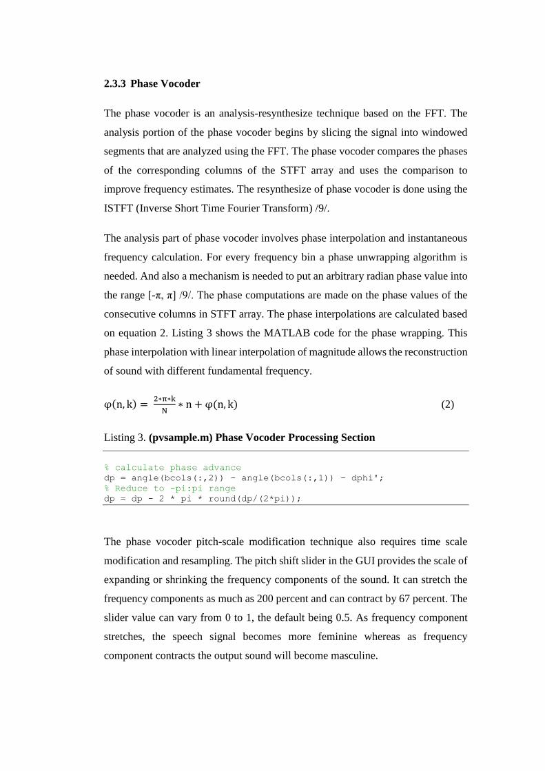
2.3.3 Phase Vocoder

The phase vocoder is an analysis-resynthesize technique based on the FFT. The

analysis portion of the phase vocoder begins by slicing the signal into windowed

segments that are analyzed using the FFT. The phase vocoder compares the phases

of the corresponding columns of the STFT array and uses the comparison to

improve frequency estimates. The resynthesize of phase vocoder is done using the

ISTFT (Inverse Short Time Fourier Transform) /9/.

The analysis part of phase vocoder involves phase interpolation and instantaneous

frequency calculation. For every frequency bin a phase unwrapping algorithm is

needed. And also a mechanism is needed to put an arbitrary radian phase value into

the range [-π, π] /9/. The phase computations are made on the phase values of the

consecutive columns in STFT array. The phase interpolations are calculated based

on equation 2. Listing 3 shows the MATLAB code for the phase wrapping. This

phase interpolation with linear interpolation of magnitude allows the reconstruction

of sound with different fundamental frequency.

φ(n, k) = 2∗π∗k

N∗ n + φ(n, k) (2)

Listing 3. (pvsample.m) Phase Vocoder Processing Section

% calculate phase advance dp = angle(bcols(:,2)) - angle(bcols(:,1)) - dphi'; % Reduce to -pi:pi range dp = dp - 2 * pi * round(dp/(2*pi));

The phase vocoder pitch-scale modification technique also requires time scale

modification and resampling. The pitch shift slider in the GUI provides the scale of

expanding or shrinking the frequency components of the sound. It can stretch the

frequency components as much as 200 percent and can contract by 67 percent. The

slider value can vary from 0 to 1, the default being 0.5. As frequency component

stretches, the speech signal becomes more feminine whereas as frequency

component contracts the output sound will become masculine.

19

Compressing or stretching the frequency components will not affect the duration of

the audio signal. The expansion and compression of the frequency spectrum takes

place during the resampling stage. Since this approach is linear by its nature, all the

frequencies in the signal will end up multiplying by the same factor. As a result,

harmonizing a signal requires repeated processing, which might be expensive

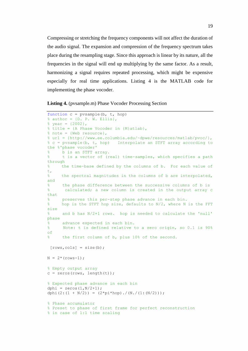
especially for real time applications. Listing 4 is the MATLAB code for

implementing the phase vocoder.

Listing 4. (pvsample.m) Phase Vocoder Processing Section

function c = pvsample(b, t, hop)

% author = {D. P. W. Ellis},

% year = {2002},

% title = {A Phase Vocoder in {M}atlab},

% note = {Web resource},

% url = {http://www.ee.columbia.edu/~dpwe/resources/matlab/pvoc/},

% c = pvsample(b, t, hop) Interpolate an STFT array according to

the %'phase vocoder' % b is an STFT array. % t is a vector of (real) time-samples, which specifies a path

through % the time-base defined by the columns of b. For each value of

t, % the spectral magnitudes in the columns of b are interpolated,

and % the phase difference between the successive columns of b is % calculated; a new column is created in the output array c

that % preserves this per-step phase advance in each bin. % hop is the STFT hop size, defaults to N/2, where N is the FFT

size % and b has N/2+1 rows. hop is needed to calculate the 'null'

phase % advance expected in each bin. % Note: t is defined relative to a zero origin, so 0.1 is 90%

of % the first column of b, plus 10% of the second.

[rows,cols] = size(b);

N = 2*(rows-1);

% Empty output array c = zeros(rows, length(t));

% Expected phase advance in each bin dphi = zeros(1,N/2+1); dphi(2:(1 + N/2)) = (2*pi*hop)./(N./(1:(N/2)));

% Phase accumulator % Preset to phase of first frame for perfect reconstruction % in case of 1:1 time scaling

ph = angle(b(:,1));

% Append a 'safety' column on to the end of b to avoid problems % taking *exactly* the last frame (i.e. 1*b(:,cols)+0*b(:,cols+1)) b = [b,zeros(rows,1)];

ocol = 1; for tt = t % Grab the two columns of b bcols = b(:,floor(tt)+[1 2]); tf = tt - floor(tt); bmag = (1-tf)*abs(bcols(:,1)) + tf*(abs(bcols(:,2))); % calculate phase advance dp = angle(bcols(:,2)) - angle(bcols(:,1)) - dphi'; % Reduce to -pi:pi range dp = dp - 2 * pi * round(dp/(2*pi)); % Save the column c(:,ocol) = bmag .* exp(j*ph); % Cumulate phase, ready for next frame ph = ph + dphi' + dp; ocol = ocol+1; end

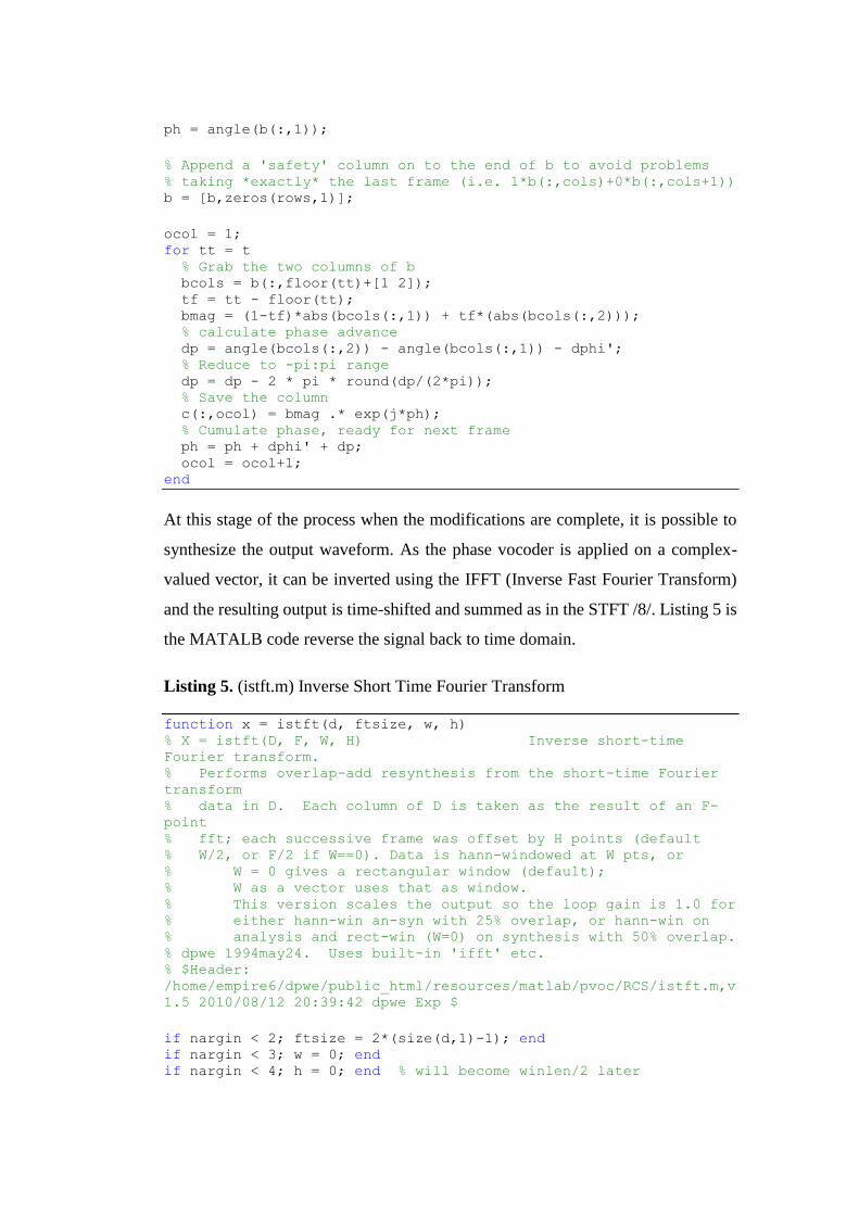
At this stage of the process when the modifications are complete, it is possible to

synthesize the output waveform. As the phase vocoder is applied on a complex-

valued vector, it can be inverted using the IFFT (Inverse Fast Fourier Transform)

and the resulting output is time-shifted and summed as in the STFT /8/. Listing 5 is

the MATALB code reverse the signal back to time domain.

Listing 5. (istft.m) Inverse Short Time Fourier Transform

function x = istft(d, ftsize, w, h) % X = istft(D, F, W, H) Inverse short-time

Fourier transform. % Performs overlap-add resynthesis from the short-time Fourier

transform % data in D. Each column of D is taken as the result of an F-

point % fft; each successive frame was offset by H points (default % W/2, or F/2 if W==0). Data is hann-windowed at W pts, or % W = 0 gives a rectangular window (default); % W as a vector uses that as window. % This version scales the output so the loop gain is 1.0 for % either hann-win an-syn with 25% overlap, or hann-win on % analysis and rect-win (W=0) on synthesis with 50% overlap. % dpwe 1994may24. Uses built-in 'ifft' etc. % $Header:

/home/empire6/dpwe/public_html/resources/matlab/pvoc/RCS/istft.m,v

1.5 2010/08/12 20:39:42 dpwe Exp $

if nargin < 2; ftsize = 2*(size(d,1)-1); end if nargin < 3; w = 0; end if nargin < 4; h = 0; end % will become winlen/2 later

21

s = size(d); if s(1) ~= (ftsize/2)+1 error('number of rows should be fftsize/2+1') end cols = s(2);

if length(w) == 1 if w == 0 % special case: rectangular window win = ones(1,ftsize); else if rem(w, 2) == 0 % force window to be odd-len w = w + 1; end halflen = (w-1)/2; halff = ftsize/2; halfwin = 0.5 * ( 1 + cos( pi * (0:halflen)/halflen)); win = zeros(1, ftsize); acthalflen = min(halff, halflen); win((halff+1):(halff+acthalflen)) = halfwin(1:acthalflen); win((halff+1):-1:(halff-acthalflen+2)) =

halfwin(1:acthalflen); % 2009-01-06: Make stft-istft loop be identity for 25% hop win = 2/3*win; end else win = w; end

w = length(win); % now can set default hop if h == 0 h = floor(w/2); end

xlen = ftsize + (cols-1)*h; x = zeros(1,xlen);

for b = 0:h:(h*(cols-1)) ft = d(:,1+b/h)'; ft = [ft, conj(ft([((ftsize/2)):-1:2]))]; px = real(ifft(ft)); x((b+1):(b+ftsize)) = x((b+1):(b+ftsize))+px.*win; end;

2.4 Reverberation

2.4.1 Background

The world we live in is composed of reverberant materials. Whether we are

enjoying a musical performance in a concert hall, speaking to colleagues in the

office, walking outdoors on a city street, or even in the woods, delayed reflections

from many different directions always accompany the sound we hear /2/. Often

these events go unnoticed, let alone causing confusion, because the human hearing

system is designed for such acoustic environment. If the reflections happen shortly

after the initial sound, the sound will not be distinguishable as the same sound

arrives at different time. Instead, the reflections enhance the perception of the

sound, by changing the loudness and the spatial characteristics of the sound. In a

highly reverberant environment late reflections are very common. Concert halls and

cathedrals are good examples of the effect of background ambience, which is quite

different from the foreground sound.

The importance of reverberation in recorded music and other acoustic applications

has brought the creation of artificial reverberator. The availability of digital

electronic devices in such amount and price has made reverberation a ‘must add’

effect in the audio production industry. These days, recordings, radio, television,

and movies have the effect of artificial reverberation.

The artificial reverberator was first created by Manfred Schroeder and Ben Logan.

Since then various scientists contributed to the advancement of the reverberator.

This chapter is about Schroeder’s reverberator. The parallel structure of four comb

filters feeding the signal to two cascaded All-Pass filters has been created in the

MATLAB environment, as shown in Figure 3.

2.4.2 Approaches to Reverberation Algorithm

The reverberator is a linear discrete-time system that simulates the input-output

behavior of a real or imagined room /2/. We can approach, when designing a

reverberator, either from the physical or perceptual point of view.

The physical approach tries to simulate the propagation of sound from the source

to the listener for a given room. This is done by calculating the binaural system

responses of the given room, and then reverberation can be calculated by

convolution.

When the room does not exist, we then have to predict the impulse response from

the physical point of view. This may need deep knowledge about the types of wall

23

finish, ceilings, floors as well as the shape of the room to recreate the possible

propagation of the sound. The position and directives of the sound source and the

listener should also be taken into consideration.

One advantage of this method is that it lets us simulate the exact propagation and

perception of sound in the given environment. However, this approach needs lots

of calculation before it renders the effect, and also it is inflexible.

Perceptual approach, on the other hand, tries to recreate reverberation using only

the perceptual salient characteristics of sound propagation. The design takes place

by assuming, N different sound signals which are reflected from N different objects

cause the reverberation. Then our task would be designing a digital filter with N

parameters that reproduces exactly those N attributes. The reverberator should then

produce reverberation that is indistinguishable from the original, even though the

fine details of the impulse response may differ considerably /2/. This approach is

used in the design of Schroeder’s reverberator.

2.4.3 Early Reverberation

When the produced sound radiates out of the sound source, it reaches the listener in

two ways. Either it travels directly in the direction of the listener or it reaches the

listener after bouncing back from different surfaces. If the reflection delay is longer

than 80 milliseconds, the reflection will be recognized as a detached echo from the

direct sound if it is loud enough.

As the reflection delay gets shorter, the direct and the reflection sound integrate to

form one sound. This may increase the loudness of the direct sound. For small

reflection delay, if less than 5 millisecond, the echo can cause the apparent location

of the source to shift. Longer delays can increase the apparent size of the source,

depending on its frequency content, or can create the sensation of being surrounded

by sound /2/.

2.4.4 Schroeder’s Reverberator

In 1960 Dr.Schroeder came up with the first artificial reverberator. He implemented

the reverberator based on digital signal processing concepts. Schroder's

reverberator is much simpler reverberator especially compared to today's

commercial reverberator. Schroeder's reverberator uses 4 comb filters arranged in

parallel followed by two cascaded all-pass filters.

Figure 2. Schematic diagram of Schroeder reverberator

The comb filter shown in Figure 3 consists of a delay whose output is fed back to

the input. The Z transform of the comb filter is given by the following equation:

𝐻(𝑧) = 𝑧−𝑚

1−𝑔𝑖∗𝑧−𝑚 (3) /2/

Where m is the length of the delay in samples and gi is the feedback gain. The gain

coefficients can be calculated using the following formula

𝑔𝑖 = 10(−3∗𝑚∗𝑇)

𝑇𝑟 (4) /2/

Reverberation time (Tr) dictates the value of gains in the comb filters. The optimum

reverberation time for an auditorium or room depends on its intended use.

Reverberation time of 2 seconds is usually good for the general purpose auditorium

for both speech and music /2/. T is for the sampling period. The MATLAB voice

processing demo project has 8000 sampling frequencies to record a speech signal;

that would give a sampling period of 0.125 millisecond.

25

Schroeder recommended that the ratio of largest to smallest in the delays of comb

filter to be about 1.5. Making the shortest delay 27ms the longest one would be

41ms. The four comb filters then have a delay of 27ms, 33ms, 37ms, and 41ms.

Figure 4 shows the schematic diagram while Listing 6 is the MATLAB code for

comb filter.

Figure 3. Comb filter /11/

Listing 6. (comb.m) Comb filter

function y = comb(sound_signal,fs) %COMB Filters input sound_signal and returns output y. delay1 = 0.027*fs;%27ms delay delay2 = 0.033*fs;%33 ms delay delay3 = 0.037*fs;%37 ms delay delay4 = 0.041*fs;%41 ms delay Tr = 2; %reverberation time g1 = 10^((-3*delay1*1/fs)/Tr);%-0.911; g2 = 10^((-3*delay2*1/fs)/Tr);%-0.892; g3 = 10^((-3*delay3*1/fs)/Tr);%-0.88; g4 = 10^((-3*delay4*1/fs)/Tr);%-0.868; persistent Hd1; if isempty(Hd1) % The following code was used to design the filter

coefficients: % N = 216; % Order Q = 16; % Q-factor h1 = fdesign.comb('Peak', 'N,Q', N, Q); Hd1 = design(h1); end y1 = filter(Hd1,sound_signal); persistent Hd2; if isempty(Hd2) % The following code was used to design the filter

coefficients: N = 264; % Order

Q = 16; % Q-factor h2 = fdesign.comb('Peak', 'N,Q', N, Q); Hd2 = design(h2); end y2 = filter(Hd2,sound_signal);

persistent Hd3; if isempty(Hd3) % The following code was used to design the filter

coefficients: % N = 296; % Order Q = 16; % Q-factor h3 = fdesign.comb('Peak', 'N,Q', N, Q); Hd3 = design(h3); end % y3 = filter(Hd3,sound_signal); persistent Hd4; if isempty(Hd4) % The following code was used to design the filter

coefficients: N = 328; % Order Q = 16; % Q-factor h4 = fdesign.comb('Peak', 'N,Q', N, Q); Hd4 = design(h4); end y4 = filter(Hd4,sound_signal); y = y1+y2+y3+y4+sound_signal; clear Hd1 Hd2 Hd3 Hd4;

The all-pass delays are much shorter than the comb delays in the comb filter. The

delay time of 5 and 1.7millisecond would be enough for both all-pass filters. The

all-pass gains have the value of 0.7. There are some drawbacks associated with the

series association of all-pass filters. To mention a few, as the order of the filter gets

higher, the time it takes for the echo density to build up to a pleasing level will also

increase. In addition, the higher order all-pass filters usually exhibits an annoying,

metallic ringing sound /2/.

The Z transform of a series connection of two all-pass filters is governed by the

formula 5:

𝐻(𝑧) = ∏0.7−0.7∗𝑧−𝑑𝑒𝑙𝑎𝑦

0.7−0.7∗𝑧−𝑑𝑒𝑙𝑎𝑦2𝑖=1 (5) /2/

27

Figure 4. All-Pass filter /10/

Listing 7. (allpass_function.m) All-Pass filter

function [ y ] = allpass_function( M,fs ) %UNTITLED Summary of this function goes here % Detailed explanation goes here delay1 = floor(0.005*fs);%5msec delay delay2 = floor(0.002*fs);%2msec delay

g5 = 0.35; g6 = 0.35;

d = zeros(length(M),1); p = zeros(length(M),1); f = zeros(length(M),1); y = zeros(length(M),1);

d(1) = M(1); for n = 2:length(M) if(n <= delay1) d(n) = M(n) + p(n-1)*g5; p(n) = -g5*M(n); end if(n > delay1) d(n) = M(n) + p(n-1)*g5; p(n) = -g5*M(n) + d(n-delay1); end end f(1) = p(1); for n = 2:length(M) if(n <= delay2) f(n) = p(n) + y(n-1)*g6; y(n) = -g6*p(n); end if(n > delay2) f(n) = p(n) + y(n-1)*g6; y(n) = -g6*p(n) + f(n-delay2); end end % fvtool(y); end

3 MATLAB GUI

3.1 Background

A graphical user interface (GUI) is a user-friendly mechanism between an

application and a user. A GUI gives an application a distinctive appearance and

processing approach. GUI is made from GUI components. These GUI components

are sometimes referred to as controls. A GUI component is an object with which

the user communicates with the application using the computer input devices, such

as mouse and keyboard. The user of the GUI does not have to create a script or

write commands at the command prompt to accomplish the task. The user of a GUI

does not need to understand the details of the process behind the GUI component.

The GUI components can include menus, toolbars, pushbuttons, radio buttons, list

boxes, and sliders. GUIs created by using MATLAB tools can be made capable of

performing complicated computations, reading and writing data into and from the

files. Intercommunication among GUIs and displaying data either in table format

or plot is also achievable.

In this project of voice processing pushbuttons, radio buttons, text boxes, slider and

drop down menus were used. These components are coherently interrelated with

each another. This chapter describes the inter-relation of the different components

and the effect they can bring on the signal being processed.

3.2 Programming GUI Application in MATLAB

By its very nature, a GUI will not take any action unless the user invokes. The GUI

reaction will trigger the appropriate function as its response to the action taken by

the user. Each control within the GUI has one function generated by the MATLAB

automatically. This MATLAB function is known as callback. These callback

functions can do the job by themselves or they in turn may call other functions to

distribute the workload and for the clarity of the code.

29

The user action always initiates callbacks to be executed. This action can be

pressing a push button, typing digits in the text field, or it could be selecting a menu

item.

The program remains idle unless it is invoked by some external event, this type of

programming is said to be an event driven programming. In the event driven

programming, events can occur in asynchronous manner, meaning they occur

randomly. In the voice processing demo project, all events happen by the user

interactions with the GUI.

3.3 How to Build MATLAB GUI

A MATLAB GUI is a figure window with an adjustable size and position. The

callback functions will make the component do with mouse clicks and keystrokes.

A MATLAB GUI can be built in two ways /3/:

- Using GUIDE (Graphical User Interface Development Environment)

- Programmatic GUI construction

GUIDE creates a figure from the graphic layout editor along with the corresponding

code file. The code file is composed of a series of callback and creates functions for

GUI components. GUIDE provides a set of tools for creating graphical user

interfaces (GUIs). These tools greatly simplify the process of laying-out and

programming GUIs /3/. This voice processing demo project is developed based on

this method.

The second method, the programmatic approach creates a code file that defines all

component properties and behaviors. Whenever the file runs, it creates the figure.

The components and handles will then take their positions in the figure. Every time

the code runs, it creates a new.

3.4 Comparing the Two Versions of Voice Processing Tool

This voice processing demo project was developed based on another voice

processing tool developed by Dr. Gao Chao. A comparison between the newer

version and the older version shows pleasing similarities and differences. The GUI

appearance is perhaps the most obvious difference between the two versions. The

newer version displays the graphs which represent signals on a separate window to

give the main window a tidy look. The raw and processed signals use separate

windows. As a result, we can compare visually how the process affects the signal.

Beside their different appearances, both employ the similar filter technique to

remove the unwanted signals. On the pitch shift module of the project, they both

are developed based on the works of Colombia University /16/. However, some

work has been done so as to make some improvement from the original version. In

the spectrogram drawing functions the newer version employed the MATLAB own

tool so as to bring a good and clear spectrogram drawings.

The reverberation section does not take anything from the version 1 of voice

processing tool. New functions have been added so as to recreate the original

Schroeder reverberator. The voice regulator was also added to the project which

was not there before.

The major difference in my opinion is the way the components interrelate with each

other in the newer version. The previous version was capable of doing only one

module at one instance of processing. This was a huge drawback for the tool. To

rectify this problem the newer version cascades the different modules and as a result

the user can get the combined effect of all the modules there is in the tool. All in

all, this demo voice processing tool can be considered as the next version of the

previous voice processing tool. Figures 1 and 2 show the user interfaces of the

previous and new versions of voice processing tools.

3.5 The GUI’s Task

This MATLAB voice processing tool GUI can be grouped into five categories: the

data center section, the filter section, sound processing and the graph section. The

data section of the GUI is responsible for getting the sound data. Its responsibility

is getting the sound data either by browsing through the folders for Waveform

Audio File Format (*.wav) files or by recording sound for 5 seconds. It is not

possible for the user to lengthen or shorten the time frame of recording. The “Load”

31

and “Record” buttons do the work of loading the sound data to the program. The

buttons “Play Original Sound”, “Save Original Sound” and “Reset” buttons, play

or save the sound data. The “Reset” button reset the settings of the program to the

default mode.

The filter section of the GUI is composed of four radio buttons, one for each type

of filters. Whenever one turns the radio button on, the respective text box will also

be activated. Similarly, turning the radio button off will deactivate the respective

text box. As Hertz (Hz) is the SI unit for frequency, all the input values are

understood by the program as a Hertz value. Band Pass and Band Stop Filters will

take two values to process. As to which text box to receive the higher and which

the lower frequency; no restriction has been put, so the user can freely enter values.

The program will recognize the higher value and proceeds to the process without

any problem. If the user feeds similar values for the cutoff frequencies, the program

will understand as having a 50Hz difference between the two values irrespective of

the user input value.

There are two sections in the GUI which are named as Sound Processing sections.

The Sound Processing section includes pitch shifting slider, reverb and volume

radio buttons with volume text box. The pitch shifter slider always starts at the

middle when the program loads. In order to bring some effect on the sound either

we should press the left or right arrows on either end of the slider. Pressing the

arrows will increase or decrease the values by 0.1 step value. Pressing the right

arrow increases the value thereby decreasing the fundamental frequency of the

sound being processed and that will give a masculine sound in the output signal.

The left arrow, on the other hand, increases the fundamental frequency, thereby

giving feminine sound characteristics to the output sound signal if the sound being

processed is a speech signal.

The reverb radio button when activated will bring an auditorium sound effect on

the sound signal that is being processed. Much effort was exerted to recreate the

original Schroeder reverberator. The final component of the sound processing

section is volume. This component is composed of a radio button and a text box.

Once the radio button is ‘On’, the text box will be ready to take the value. The

program understands the value in the text box as a decibel value. If the positive

value is entered then the program will increase the power of the sound signal

according to the value and if the value is negative then it will decrease the power

accordingly.

To the left side of the sound processing section there are three buttons, labeled as

“Process”, “Play Processed Sound”, and “Save Processed Sound”. Once the

“Process” button is pressed, all the selected effects from different sections of the

GUI will start to affect the signal one by one in a cascaded manner according to the

values the use entered. When the program finishes processing, the “Processed

Signal” drop down menu in the graph section of the GUI will be activated for

selection. The “Play Processed Sound” button plays the output signal, while the

“Save Processed Signal” button will let the user to save the final piece of the signal.

The graph section of the GUI is made of two dropdown menus. Whenever there is

some data to be processed, the raw signal drop down menu will be activated, but

the processed signal drop down menu will only be after the desired process is

completed. Each menu has three options to choose from. The signal representation

in time domain, in frequency domain and the spectrogram of the audio signal. The

selected figure will create a new window and draws the intended graph on the new

window. The raw signal and processed signal drop down menus can create new

windows separately- This is done so as to keep the option of comparing the effect

the different component has brought to the signal visual as it was also in voice

processing tool version 1. Changing the selection from the menus will not create a

new window, instead the selected type of graph will replace the existing one.

Figure 8 depicts the hierarchical arrangement of the different components of the

GUI. As described the above paragraphs the components are interrelated with each

other, this interrelation is presented graphically in Figure 8.

33

Figure 5. The activation hierarchy

3.6 Looking In depth Each Sections of the GUI

3.6.1 Data Center Section

Figure 9 shows the data section of the GUI. To make the explanation more visual

the detailed process of the callback functions are presented along with the flowchart

of the process triggered by the buttons.

Figure 6. The Data section of the GUI

3.6.1.1 Load Push Button

Pressing the "Load" push button triggers the "load_button_Callback" function. This

function starts its job by declaring a global variable for the sampling frequency and

a global array for the sound signal that is about to be loaded to the program. It is

very important to clean the arrays by emptying their contents. This is done in case

of loading another sound data without erasing the previously processed data using

the reset button.

After the completion of this initial stage, the function uses the UI (user interface)

capabilities of MATLAB to let the user browse through the folder. Once the desired

data has been loaded to the global array, function completes its task by setting the

parameters which are necessary for enabling or disabling the controls of the GUI.

3.6.1.2 Record Push Button

The “record_button_Callback” function is the event triggered by the “Record” push

button. Like the load_button_Callback function it declares the global variable “fs”

for sampling frequency and “LOADED_RECORDED” array for the sound signal.

It also clears the contents of LOW_PASS, HIGH_PASS, BAND_PASS,

BAND_STOP, PITCHED, AMPLIFIED and ECHOED arrays for stability of the

program. If the user tries to record sound just after the program processes another

task, then those arrays will have the contents that make it difficult for the program

to rewrite data over when it needs to change their size. The RECORD_SOUND

array is also declared here as a local array. The purpose of this local array is to carry

the recorded data from the soundObject then it transfers the transposed version of

data to the LOADED_RECORDED global array.

The program uses the audiorecorder function which is a MATLAB function to

record the speech signal. This function takes three arguments sampling frequencies,

the number of bits per sample and number of channel. A human being can generate

a sound signal up to 4000 Hz based on this fact and following the Nyquist sampling

theorem the program uses 8000Hz as sampling frequency. The program uses 16 bits

per sample for the second argument and ‘1’ to indicate the sound being recorded is

in mono channel for the third argument.

The audiorecorder function returns a soundObject which is ready to carry the

recorded data, therefore another MATLAB own function should be used which is

recordblocking to record the sound signal. The recordblocking function takes two

35

arguments and returns nothing. The soundObject which is returned by the

audiorecorder function is the first argument the function takes. While the other

argument is the length of recording in seconds. This program is set to record for 5

seconds, therefore ‘5’ is set to the recordblocking function as the second attribute.

LOADED_RECORDED array takes transposed data of the

RECOREDED_SOUND array. When the recordblocking object records the sound

signal without interruptions, it records the sound with much better clarity and

quality. Listing 8 is the MATLAB code that records sound signal.

Listing 8. (Main_window.m) Record the sound signal

fs = 8000; bits = 16; channel = 1; h = Recording('Main_window',handles.figure); set(hObject,'Value',1);

soundObject = audiorecorder(fs,bits,channel); recordblocking(soundObject,5); RECORDED_SOUND = getaudiodata(soundObject); % RECORDED_SOUND = wavrecord(5*fs,fs,channel);

LOADED_RECORDED = [LOADED_RECORDED RECORDED_SOUND'];

delete(h); % DELETE the waitbar; don't try to CLOSE it.

Figure 10 shows the flow chart of the Load and Record push button callback

function.

3.6.1.3 Play and Save Original Sound Buttons

In figure 10 there are also three more buttons Play Original Sound, Save Original

Sound and Reset buttons in the data section of the GUI. The purpose of the Play

original sound button is to play the sound data that is loaded to

LOADED_RECORDED array. To use the array the triggered function by the button

play_ori_button_Callback function has to declare it as a global array and also the

sampling frequency should be declared as a global variable. The function uses the

sound function from MATLAB. This function takes the sound data and sampling

frequency as its two arguments and plays the data.

The Save Original Sound button also needs LOADED_RECORDED global array

and sampling frequency global variable. The MATLAB “uiputfile” function

provides the user interface means to save the file in the desired directive. The

function takes two string arguments. The first argument gives the option to select

the file format to be saved while the other is for the header of the save window

figure.

The reset push button resets all the global variables and arrays by clearing their

contents. The button triggers the Reset_pushbutton_Callback function which then

declares all the global arrays and variables to clear their contents. It also sets the

parameters of the controls to stage when the program runs for the first time. The

reset button is activated only after the program processes the data.

37

Figure 7. Flow chart for the buttons of Data Section

3.7 Filter Components

Filters are the basis of speech processing applications, therefore, this voice

processing MATLAB project includes four of the most basic types of filters. The

filters are arranged in the GUI under the Filters section. Figure 11 represents the

filter section of the GUI.

Figure 8. The Filter section

The filters are represented in the radio buttons. The radio button LPF stands for low

pass filter, HPF for high pass filter, BPF for band pass filter and BSF for band stop

filter. Whenever they are turned on the text fields, which are placed just under, the

radio button will be activated and become ready to receive values. The arrows

represent the cascaded arrangement of the program. The low pass filter is the first

to receive the data in the filter section- If it is on, then it processes the data according

to the value that is fed into the text box just underneath the radio button. On the

other hand, if it is not turned on, then it will pass the data to high pass filter without

bringing any effect into it.

The high pass filter would then be the next filter to receive the data. Like LPF it

processes the data based on the value there is in the text field associated with it,

otherwise it will just pass the data to the band pass filter. In the similar the fashion

band pass and band stop filters will handle their tasks.

The radio buttons are also connected with a callback function. The radio button LPF

is connected to the LPF_radiobutton_Callback function and HPF with the

HPF_radiobutton_Callback function, BPF with the BPF_radiobutton_Callback

function and BSF with the BSF_radiobutton_Callback function. Figure 11 shows

the interactions there are among the radio buttons in the filter section of the GUI.

39

Figure 9. Flow chart for filter section radio buttons

All the four callback functions are designed in a very similar manner. They use

flags for inter-communication among the radio buttons. This inter-communication

is essential in the case the user changes its mind. When the radio buttons are on, the

process button becomes active. When the radio button is off, it will freeze the

process button after checking the status of other activating components. That is to

say, there is an inner communication mechanism among the activation components

of the GUI.

3.8 Sound Processing Section

This section includes Pitch shifting slider, Reverb and Volume radio buttons with

Volume text box. The algorithm behind of pitch shifting and reverberation has been

discussed under the subheadings of 2.3 and 2.4. Figure 13 shows the sound

processing section of the GUI.

Figure 10. The sound processing section of the GUI

3.8.1 Pitch Shift Slider

The pitch shift slider invokes the pitch_slider_Callback function. The chief target

for the function is to activate the status of process pushbutton and reset push button.

The mechanism it does this is very similar to that of the callback functions of radio

buttons. If the value of the slider is different from 0.5, that will activate the process

push button. On the other hand when its value is equal to 0.5, then the program has

to check the status of radio buttons before it deactivates the process and reset

buttons. Figure 14 is the flow chart of the pitch_slider_Callback function.

41

Figure 11. Flow chart for pitch_slider_Callback function

3.8.2 Reverb and Volume Radio Buttons

The reverb and volume radio buttons are designed to do similar job as filter radio

buttons which are explained in section 3.7.

3.8.3 Process Pushbutton

The process push button calls the functions process_pushbutton_Callback function.

This function like any other MATLAB callback functions begins with declaring

global variables. In MATLAB global variables need to be declared under the figure

opening function. The name of this function is Main_window_OpeningFcn. They

should also be re-declared under the callback functions. Otherwise, the program

would not recognize them as a global variable, instead they will be treated as a local

variable.

After the declaration of global variables, parameter setting and local variable

declaration will follow. The program cascades the function exactly as the arrow

show in the GUI. Therefore, the process_pushbutton_Callback function will check

the status and do the required analysis and process one by one starting from the low

pass filter and ends at the volume radio button in the sound processing section.

The flags associated with the radio buttons are the ones which indicate the callback

function whether the radio button is selected or not. If so it brings the value from

the edit text boxes in the case of filters and volume or bring the value of slider in

the case of the Pitch shift slider to process the request.

Each processing units in the structure has a corresponding global array.

LOADED_RECORDED associated with the load and recorded sound data.

LOW_PASS array will be filled with data after the low pass filter unit. If the low

pass filter is not selected, then the LOADED_RECORDED content will be copied

to the LOW_PASS array. HIGH_PASS is with the high pass filter. If it is selected,

then the highpass MATLAB function will filter the signal, otherwise the contents

of the LOW_PASS array will be copied to the HIGH_PASS array. In the similar

fashion BAND_PASS is associated with the band pass filter, BAND_STOP is with

43

the band stop filter. All of the filters use MATLAB own filter functions lowpass,

highpass, bandpass and bandstop functions.

Similarly, the PITCHED global array is associated with the pitch shift unit of the

program. Following Pitch shifting there is ECHOED for reverb and AMPLIFIED

for volume.

Figure 12. Flow chart for process pushbutton

3.9 Graph Section

The Graph Section of Voice Processing GUI consists of two drop down menus. One

capable of plotting raw signal, while the other plots the processed signal. Each drop

45

down menu consists of three options for the three type of figures they are capable

of plotting. Figure 16 represents this section of the GUI.

Figure 13. The Graph section

The Raw Signal drop down menu or as MATLAB calls it popup menu triggers the

input_popupmenu_Callback function. This function begins by declaring the global

variable sampling frequency and global array LOADED_RECORDED. All the

three graphs need them. The function after getting the selected figure from the user

will call the Raw_Signal function. This Raw_Signal is a figure by itself, which is

made of a title bar and an axis.

The Raw_Signal function or figure will call the figures function and pass the

parameters it receives from the parent figure Main_Window. The functions of the

figure based on the value of the selected figure will draw the appropriate graph. If

the value of the selected figure is from 2 to 4, then it plots the signal for Raw_Signal

function. Whereas, if the value is from 5 to 7 then it plots the signal for

Processed_Signal function.

If the value of the selected figure is 2 or 5, then the signal to be plotted is in time

domain. The horizontal axis is for the time in seconds, while the vertical axis is for

the amplitude of the signal. ‘1’ is the maximum value the amplitude can go to while

‘-1’ is the minimum value it can possibly have. Figure 17 shows the plot of a flute

melody as plotted by the figures function and displayed by the Raw_Signal figure

window.

Figure 14. Sound signal in time domain

Whereas if the value of the selected figure is 3 or 6, then the output will be the plot

of the signal in the frequency domain. Naturally, all the recorded or stored sound

signals are in the time domain. Transforming the signal from time to frequency

domain is done through DFT techniques. Analyzing, manipulating and

synthesizing signals are much handy in the frequency domain. To plot the Fourier

Transform of the sound signal the FFT algorithm was used. This algorithm provides

a technique which simplifies the complexity and length that would be necessary had

the direct DFT formula been employed. Then the horizontal axis in the plot

represents the frequency of the signal while the vertical axis the cumulative sum of

the amplitude of the signal. Figure 18 shows the frequency spectrum of the sound

signal plotted in the Figure 17.

47

Figure 15. Frequency spectrum of the sound signal

The final case is when the selected figure is either 5 or 7. In such a case the

spectrogram graph would be plotted. The spectrogram is considered a very

informative way of plotting a signal. This is because it uses three axes to plot the

signal whereas the frequency spectrum and time domain uses two. The vertical axis

represents time in seconds, the horizontal axis is for the frequency in hertz and the

third axis is for the amplitude of the signal which is represented by the intensity and

type of color.

The color map chosen is ‘jet’ color map. In this color map the lowest amplitude has

the deep blue color changes to cyan then to yellow, red, and finally to dark red for

those frequencies with the highest amplitude. The color change follows a linear

pattern as it goes from deep blue to dark red.

MATLAB has its own function which can draw a spectrogram plot. This function

takes sound data, window length, hop length, FFT length, and sampling frequency

of the signal. In return, it plots the spectrogram of the sound data. Figure 19 is the

spectrogram of the flute melody as drawn by the program and displayed by the

Raw_Signal figure window.

Figure 16. Spectrogram of the sound signal

49

4 CONCLUSION

This thesis is about improving the version 1 voice processing demo MATLAB

project. During this improvement some features are added and some functions are

improved in this sense the thesis achieved its aim. The pitch shifter implementation

is largely based on the works of Colombia University. Part of the code was

borrowed from their website /16/. Implementation of reverberation section is made

based on the theory set by the Kahrs Mark and Karlheinz Brandenburg book /2/.

All other features are made based on MATLAB own reference books /3/ /4/.

Voice processing is a very deep subject. It is rooted deeply in advanced mathematics

and signal processing techniques. This project can be seen as a gateway or entry

level for speech processing applications. Yet, it is challenging enough if someone

does not have a concrete knowledge on the speech processing subject.

I believe that I have gained huge experience from this project. There was an

immense amount of research in order to understand the core subject of the project,

speech processing. MATLAB has been the first choice tool among digital signal

processing engineers for its high computational capability. The project also tries to

capitalize on the GUI capability of MATLAB. Combining the two tools of

MATLAB has given me a good hands-on experience about the nature of projects.

From a research perspective, I covered lots of materials from standard course books

to research papers. I began covering the subject from signal and systems, then

digital signal processing, finally speech processing. I followed a direct approach in

solving the task at hand. I started engaging in the implementation phase only after

I thoroughly understood the theory. Through the process, I learnt that this approach

is not applicable for projects with tight schedules, but if time is not the issue, it will

always give a ripe fruit at the end.

The thesis was a good tool in developing time management skills in relation to

handling a project. In addition to that, the perspective I have for projects matured

as well as coordinating the different components of a single project.

The future of voice processing seems reasonably bright. During the process of this

thesis, many issues have been found to be potential topics for further research work.

For that reason, the following issues raised for further developments.

- A Speech recognition system: Speech to text conversion is the process

which plays a very important role specially for hearing impaired

individuals. It is also applicable in subtitling, automatic translation, court

reporting, telematics, military and others.

- A Speaker recognition system: This process of identifying the speaker

from its speech signal has applications in authenticating the identity of a

speaker as part of the security process.

51

5 REFERENCES

/1/ Flanagan.J.L. And R.M.Golden. 1966, Phase Vocoder

/2/ Kahrs, Mark, Karlheinz Brandenburg. 1998, Applications of digital signal

processing to audio and acoustics

/3/ MATLAB, R2012a. MATLAB Creating Graphical User Interfaces

/4/ MATLAB, R2012a. Signal Processing Toolbox User’s Guide

/5/ Palamides, Alex & Anastasia Veloni. 2010, Signals and Systems Laboratory

with MALAB

/6/ Rabinar.L.R. And R.W.Schafer. 1978, Digital Processing of Speech Signals

/7/ Schilling, Robert J. & Sandra L. Harris. 2011, Digital Signal Processing With

MATLAB

/8/ Sethares,William A. 2007, Rhythm and Transforms

/9/ Zölzer, Udo. 2011, DAFX: Digital Audio Effects Second Edition

/10/ All-pass filter. Accessed 20.4.2013. http://cnx.org/content/m11657/latest/

/11/ Comb filters. Accessed 19.4.2013.

https://ccrma.stanford.edu/~jos/pasp/Feedback_Comb_Filters.html

/12/ Digital filter. Accessed 19.4.2013.

http://www.mikroe.com/chapters/view/71/chapter-1-basic-concepts-of-digital-

filtering-and-types-of-digital-filters/

/13/ Pitch shifting http://en.wikipedia.org/wiki/Pitch_shift

/14/ Reverberation. Accessed 19.3.2014. http://en.flossmanuals.net/csound/e-

reverberation/

/15/ Signal Processing. Accessed 24.3.2013.

http://www.ee.columbia.edu/~dpwe/pubs/Ellis10-introspeech.pdf

/16/ Vocoder. Accessed 20.3.2014.

http://www.ee.columbia.edu/~dpwe/resources/matlab/pvoc