d0206 insa m36 - urban track · tip5-ct-2006-031312 page 1 of 85 urban track issued: 04-09-09 15:46...
TRANSCRIPT

TIP5-CT-2006-031312 Page 1 of 85 URBAN TRACK Issued: 04-09-09 15:46
D0206_INSA_M36.doc
DELIVERABLE D2.6 Related Milestone
CONTRACT N° PROJECT N° FP6-31312 ACRONYM URBAN TRACK
TITLE Urban Rail Transport PROJECT START DATE September 1, 2006
DURATION 48 months Subproject SP2 Cost effective track maintenance, renewal & refurbishment methods
Work Package WP 2.2.2a Optimal maintenance methodology
Written by S. Descartes, Y. Berthier, A. Saulot INSA Lyon
Date of issue of this report 2009/07/20 PROJECT CO-ORDINATOR Dynamics, Structures & Systems International D2S BE
PARTNERS Société des Transports Intercommunaux de Bruxelles STIB BE Alstom Transport Systems ALSTOM FR Bremen Strassenbahn AG BSAG DE Composite Damping Materials CDM BE Die Ingenieurswerkstatt DI DE Institut für Agrar- und Stadtökologische Projekte an
der Humboldt ASP DE
Tecnologia e Investigacion Ferriaria INECO-TIFSA ES Institut National de Recherche sur les Transports &
leur Sécurité INRETS FR
Institut National des Sciences Appliquées de Lyon INSA-CNRS FR Ferrocarriles Andaluces FA-DGT ES Alfa Products & Technologies APT BE Autre Porte Technique Global GLOBAL PH
Politecnico di Milano POLIMI IT Régie Autonome des Transports Parisiens RATP FR Studiengesellschaft für Unterirdische Verkehrsanlagen STUVA DE Stellenbosch University SU ZA Transport for London LONDON
TRAMS UK
Ferrocarril Metropolita de Barcelona TMB ES Transport Technology Consult Karlsruhe TTK DE Université Catholique de Louvain UCL BE Universiteit Hasselt UHASSELT BE
Project funded by the European Community under the SIXTH FRAMEWORK PROGRAMME PRIORITY 6 Sustainable development, global change & ecosystems International Association of Public Transport UITP BE
Union of European Railway Industries UNIFE BE Verkehrsbetriebe Karlsruhe VBK DE Fritsch Chiari & Partner FCP AT
Metro de Madrid MDM ES

TIP5-CT-2006-031312 Page 2 of 85 URBAN TRACK Issued: 04-09-09 15:46
D0206_INSA_M36.doc
T A B L E O F C O N T E N T S 0. Executive summary............................................................................................................................3
0.1. Objective of the deliverable ......................................................................................................3 0.2. Strategy used and/or a description of the methods (techniques) used with the justification thereof.................................................................................................................................4 0.3. Background info available and the innovative elements which were developed ............5 0.4. Problems encountered ...............................................................................................................5 0.5. Partners involved and their contribution ...............................................................................5 0.6. Conclusions .................................................................................................................................6 0.7. Relation with the other deliverables (input/output/timing) ..............................................6
1. Study of the RATP protocol for lubrication and its experiment..................................................7 2. On-site visit and characterization of the mixture .........................................................................8
2.1. Site ................................................................................................................................................8 2.2. Sampling......................................................................................................................................9 2.3. Characterizations of the mixture............................................................................................11
3. Mixture rheology..............................................................................................................................16 3.1. Tests on the “Bridgman” simulator .......................................................................................16
3.1.1. Description ........................................................................................................................16 3.1.2. Torques and friction coefficients results .......................................................................17 3.1.3. Tribological analyses........................................................................................................20 3.1.4. Synthesis ............................................................................................................................24
3.2. Tests on the “PeDeBa” simulator ...........................................................................................26 3.2.1. General experimental details ..........................................................................................26 3.2.2. Preliminary tests...............................................................................................................32 3.2.3. Study of the tribological life of mixtures.......................................................................40 3.2.4. Representativity of the tests – Parallel to wheel-rail contact reality .........................56 3.2.5. Synthesis ............................................................................................................................59
4. Numerical investigations on local wheel-rail contact characteristics .......................................61 4.1. Wheel-rail contact models and choices .................................................................................62
4.1.1. A classical 2D model of wheel-rail contact at full-scale..............................................63 4.1.2. An enhanced 2D model of wheel-rail contact at full scale .........................................67 4.1.3. A 3D model of wheel-rail contact at full-scale .............................................................68
4.2. Wheel-rail contact characteristics and parallel to reality....................................................69 4.2.1. Wheel-rail contact characteristics...................................................................................69 4.2.2. Parallel to wheel-rail contact reality ..............................................................................75
4.3. Influence of the friction coefficient, simulating under and over lubrication, on the wheel-rail contact characteristics .......................................................................................................76
5. Conclusion.........................................................................................................................................80
TIP5-CT-2006-031312 Page 3 of 85 URBAN TRACK Issued: 04-09-09 15:46
D0206_INSA_M36.doc
0. EXECUTIVE SUMMARY
0.1. OBJECTIVE OF THE DELIVERABLE
In urban rail networks, narrow curves make wheel rail lubrication an important topic. A good lubrication process reduces the wear and the friction in the wheel flange and flange root, meanwhile keeps the rail head dry for optimal adhesion. As a consequence a good lubrication reduce the maintenance cost and increase the life time with a benefit impact on security. Finding the right lubricant and setting the optimal amount of lubricant is not immediate. Indeed 18 to 24 months minimum are generally required to settle a stable lubrication process. For any change impacting the lubrication process as rolling stock refurbishment (new trains), lubricant changes (for example for greens oils), or greasing devices, a new process adjustment is needed. A bad adjustment of the lubrication process may leads to catastrophic wear with consequences such as line closure. For minimizing the lubrication process adjustment period, an investigation of rail lubrication with the purpose of reproducing the contact rheology on a reduce scale test bench is necessary. The test bench will need to respect the contact strain, geometry, and be able to reproduce the melting of lubrication oil, metallic particles (from wheels and rail) and contaminants ; this melting is hereby called "mixture". Once the test bench fulfils those conditions, the research will focus on determining the criterion that shall fulfil a good efficient lubricant. This is the work of INSA (WP2.2.2.A) to investigate rail lubrication. The research is divided in four main parts:
First INSA meets lubrication experts for the wheel-rail contact to understand how the process adjustment and the maintenance is done on RATP network. Note that RATP network has been chosen at the beginning of the project for a first investigation, especially to reduce travel costs. The tribological approach developed from RATP network study could also be transposed to others networks.
Secondly the tribological properties of the mixture is characterised. To do this, sampling are done on RATP network.
Thirdly the test benches used are described, then the formation and the tribological behaviour of the mixture investigated. The literature has reported laboratory investigations using rigs, pin-on-disk test benches and test tracks to evaluate the effect of initial lubricant on friction values and wear rates {[ALP96], [BEAG75], [CLAY89], [SUND08], [ISHI08]}. But it is the first time that the formation of the “railway” mixture, its evolution and its rheology are studied.
Fourthly a numerical model of the wheel rail contact will be settled to check that the test bench reproduce the contact strain in realistic tribological conditions. Great care will be taken to control the contact points in the aim to implement relevant tribological limit conditions. It also allows to access to local wheel-rail contact characteristics (i.e. contact positions on the rail surface, contact pressures and plastic deformations) under various lateral loading conditions from straight track to sharp curved track.
TIP5-CT-2006-031312 Page 4 of 85 URBAN TRACK Issued: 04-09-09 15:46
D0206_INSA_M36.doc
In this study, was chosen a flange root contact condition (contact angle around 45°) as a reference case.
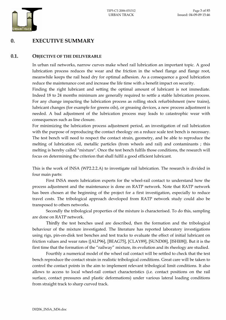
0.2. STRATEGY USED AND/OR A DESCRIPTION OF THE METHODS (TECHNIQUES) USED WITH THE JUSTIFICATION THEREOF Understanding the lubrication mechanisms involved in the wheel flange/rail gauge contact requires investigations of the tribological behaviour of the mixture. The “doped oil + detached wheel and rail particles” forms a mixture whose rheology governs the tribological behavior of the active surface – wheel flange contact (fig.1). Thus to optimize this behavior, the following strategy was used to study the rheology, formation and lifetime of this mixture.
Figure 1: Schematic view of cross-section of the wheel-rail contact
The rheology is studied under pressure (1- 3.5 GPa) and shearing with a Bridgman anvil system using a sample of mixture taken from the site. The formation, which must take into account the detachment of particles from the wheels and rails, is studied on a specific instrumented system (PeDeBa) that reproduces at reduced scale the active face-wheel flange contact (pressure, sliding, etc.). The stress fields governing particle detachment are calculated by finite elements of 100 µm x 100µm. The behavior of the mixture is taken into account by using the friction (0 – 0.3) as a parameter. The reactivity of the doped oil (oil+additives) with the particles will be studied using both the Bridgman system (surface effects) and the PeDeBa device (volume effects). The main difficulty is that the chemical composition of the additives used to dope the oil is confidential.
Globally, it is the iterative coupling between numerical and experimental (on site and on test benches) simulations that will allow progressively reconstituting the real contact conditions. This mutual enrichment is a good way to identify and so optimize the mixture’s behavior. The advantage of numerical simulation is that it is much easier to simulate the instrumentation of a contact than under experimental conditions.
Mixture (3rd body)
Contact geometry
Lubrication: initial lubricant [oil + asphalt]
Detached particles
Wear flow

TIP5-CT-2006-031312 Page 5 of 85 URBAN TRACK Issued: 04-09-09 15:46
D0206_INSA_M36.doc
This strategy involves:
- travels to sites,
- two experimental systems (one of them has to be adapted),
- surface characterization tools (Optical Microscopy, Scanning Electron Microscopies, X-ray Energy Dispersive analysis),
- numerical modeling tools (finite element mesh generator, finite element software, etc.).
The proposed approach would allow to provide tribological tools to characterize and validate a potential new lubricant in realistic contact conditions.
0.3. BACKGROUND INFO AVAILABLE AND THE INNOVATIVE ELEMENTS WHICH WERE DEVELOPED
It is now accepted {[HOU97]} that it is the rheology of the “doped oil – detached rail-wheel particles mixture” that governs the tribological behavior of the rail active flange-wheel contact. Consequently, understanding the lubrication mechanisms involved in the wheel flange/rail gauge contact requires investigations of the tribological behavior of the mixture and not only the behavior of the initial lubricant oil.
In the meantime, the tribological approach developed would be a representative and useful tribological tool for all those concerned, enabling them to validate and specify lubricants under realistic contact conditions.
0.4. PROBLEMS ENCOUNTERED
The suppliers of the doped oils want to keep the chemical composition of the additives used confidential.
The realisation of mixtures sampling on site is complex because of the low quantity of mixture and its texture gradient function of its thickness.
The project focus on the rail. Consequently information on the role of the wheels miss. This missing has been partially filled thanks to INSA previous studies (with SNCF).
The mixture is a complex melting fluid/solid. Its characterisation and its formation on a simulator are critical and require a tribological know-how.
The definition of a procedure for rail cutting out and for its transport from site to INSA, to protect the mixture from environmental contamination.
0.5. PARTNERS INVOLVED AND THEIR CONTRIBUTION
RATP, as an end-user and responsible for the maintenance of its tracks, is sharing its knowledge of network maintenance, is providing INSA with materials (for experiments and modelling) when necessary and is allowing the on-site visits.

TIP5-CT-2006-031312 Page 6 of 85 URBAN TRACK Issued: 04-09-09 15:46
D0206_INSA_M36.doc
0.6. CONCLUSIONS
It is now accepted that it is the rheology of the “doped oil – detached rail-wheel particles mixture” that governs the tribological behavior of the rail active flange-wheel contact. Consequently, a strategy combining experimental and numerical studies of the formation and rheology of this mixture has been developed. The first results make it possible to put forward a scenario of its mechanical-chemical operation. In this scenario flows of the mixture may be a means of offsetting faults in the local geometry (scale of µm to tenth of mm) of the wheels and rails and favouring different types of lubrication.
0.7. RELATION WITH THE OTHER DELIVERABLES (INPUT/OUTPUT/TIMING)

TIP5-CT-2006-031312 Page 7 of 85 URBAN TRACK Issued: 04-09-09 15:46
D0206_INSA_M36.doc
1. STUDY OF THE RATP PROTOCOL FOR LUBRICATION AND ITS EXPERIMENT
INSA has begun to analyse the RATP protocol established and controlled by a lubrication commission to understand the way rails are lubricated. Then INSA met an expert of the lubrication for the wheel-rail contact from the rolling stock department (RATP).
INSA has got main informations from the RATP expert. He has noted from his long experiment on the network a "threshold effect", which he also described as a "tribological equilibrium" of the track, is reached after grinding or new rail. When this equilibrium is stationary a specific surface aspect has been generated; it has been described as “patina”. "Patina" might mean that the "good" third body has been formed to lubricate the wheel rail contact or/and that the oil additives have reacted with the rail or third body surfaces. From our own experience, this phenomena is observed on others networks : to obtain efficient lubrication need to reconstitute a specific surface layer aspect (“right” 3rd body for lubrication).
Setting on an on-site experimental feedback, RATP has found for one initial lubricant:
• the way to create an “optimized” efficient mixture formed in situ,
• a good compromise between the contact geometry, the contact conditions and
• the conditions of lubrication (quantity, frequency).
But it will be still necessary to understand which phenomena lead to a tribological equilibrium of a track.

TIP5-CT-2006-031312 Page 8 of 85 URBAN TRACK Issued: 04-09-09 15:46
D0206_INSA_M36.doc
2. ON-SITE VISIT AND CHARACTERIZATION OF THE MIXTURE To investigate the tribological behaviour of the wheel rail contact with lubrication,
samples of mixture have been collected on rails of the RATP network. Three visits on tracks have been organised on RATP network: in January 2007, in may 2007 and in November 2007.
2.1. SITE
During the first visit, four tracks have been selected by RATP, function of their lubrication state observed by RATP experts. The lubrication of the line 3 at the chosen PK is homogeneous and good in the curve (“normal lubrication). The lubrication of the line 5 at the chosen kilometric point (PK) is not sufficient (“dry”). During this visit we have observed the specific surface aspect of the rail in the cases of good lubrication (fig. 2).
Line Inter-stations Curve radius "PK" (Localization on
the RATP line (km)) Rolling stock
(Railway dynamics)
3 République- Temple 100m on 100m 2 910 MF67
3 Opéra-4 septembre 100m on ~80m 5 300 MF67
8 République-Filles du Calvaire
Straight line 10 000 MF77
5 Oberkampf-R. Lenoir 150m on 100m 2 530 MF67-Bogie MF77
Table 1: First visit on RATP sites (January 2007)
Figure 2: Photography of the rail surface (line 3)
The second visit on site has been done on tracks of the line 3 between the stations “République” and “Temple” (track n°2), near PK 2910. The curve radius is R=100m. The length of the curve is 100m.
The third visit on site has been done on tracks of the line 8 between the stations “Invalides” and “la Tour Maubour” (track n°2), near PK 5000. The curve radius is R=75m. The length of the curve is 200m. It is a downward curve (slope= 20 mm/m) for the chosen track n° 2,
60 mm
“Optimized” efficient mixture formed in situ

TIP5-CT-2006-031312 Page 9 of 85 URBAN TRACK Issued: 04-09-09 15:46
D0206_INSA_M36.doc
i.e. from “Invalides” to “la Tour Maubourg”. The lubrication of the track is homogeneous and good. At the very end of the curve, shelling can be observed.
Line Inter-stations Curve radius
(m)
"PK" (Localization on the RATP line (km))
Rolling stock (Railway dynamics)
8 Invalides - La tour Maubourg 75
on 200m
5000 MF77
Table 2: Third visit on RATP site (November 2007)
The lubricant used in service is ejected, from the on-board greasers, on the active flange of the rail. The lubricant, which is mainly used in service, is an asphaltic oil (commercial name Vacuoline oil). But new lubricant, a biodegradable one, is also tested on line 7bis of RATP. Its commercial name is Locolub-eco.
2.2. SAMPLING
For each site and each kilometric point (PK), samples of mixture have been collected on the fillet section and on the activated flange of both rail, the inner and outer ones. The length of the collect is 400 mm, with a “spatula” (fig. 3).
Figure 3: Sampling on site
For the second visit, on line 3, samplings and photographies have been done on track 2 at PK 2920 just above a sleeper and at PK 2950 (+ 1 sleeper) (middle of the curve). Ten samples of the mixture were taken for tests in laboratory (Table 3).
For the third visit, on line 8, samplings and photographies have been done on track 2 at PK 5228 (middle of the curve) and at PK 5150 (end of the curve, in alignment), just above a sleeper. 9 samples of the mixture were taken for tests in laboratory (Table 4).
In the case of the samplings on the fillet section the thickness of the film to be collected is generally very thin (< 0.1mm). Consequently the quantity of collected mixture is too low to allow tests on rheology test bench.
After samplings on line 8, the rails have been degreased at PK 5228 and PK 5150. Then the measurements of the rails profiles at these PK have been carried out by RATP. These measurements have been done point by point, the sampling is 250 µm. The profiles measured will be used for modelling (see section 4).
Non active flange
.
Active flange
Fillet section
Length of the sampling: 400 mm
150 mm trafic

TIP5-CT-2006-031312 Page 10 of 85 URBAN TRACK Issued: 04-09-09 15:46
D0206_INSA_M36.doc
“PK”
Track 2 Low rail
(Outer rail)
High rail
(Inner rail)
Observations on site: quantity of mixture - aspect
2920
1: low - dry. 2: low - good lubrication, few quantity of particles. 3: high - presence of fibers. 4: very very low - . 5: very very low - . 6: low - few fatty.
2950 +
1 sleeper
7: low - "more fatty" than 6. 8: very low - 9: high - good lubrication, few fibers.
12: very low - more oily than the fillet section. 11: low - a little fatty. 10: little quantity - lots of particles visible, fatty.
(bold): samples for the tests on Bridgman simulator.
Table 3: First collection (2nd visit) of mixture samples – Localization on the rail and track (line 3 between the stations République and Temple (track n°2))
“PK” Track 2
Low rail (Outer rail)
High rail (Inner rail)
Observations on site: quantity of mixture - aspect
5228
15: high – fatty - light contact on this fillet section 16: low - good lubrication
17: high - very fatty 18: low – dry 19: very very low – good lubrication, very thin layer
20: very low – thin layer, plastic flow small tongue
5150
21: low – good lubrication - very thin layer 22: high - fatty
23: very very high - very oily than the fillet section
(bold): samples for the tests on Bridgman simulator.
Table 4: Second collection (3rd visit) of mixture samples – Localization on the rail and the track (line 8 between the stations “Invalides” and “la Tour Maubourg” (track n°2))
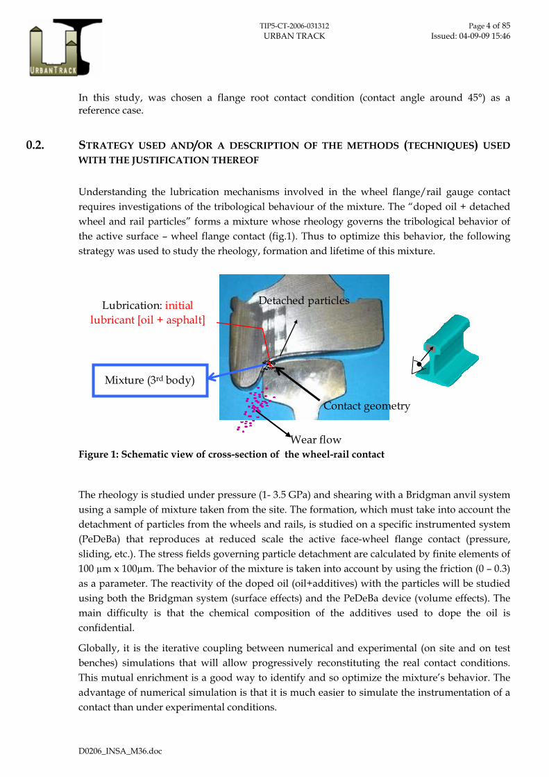
For memory and a better understanding of the next section, the schematic representation of the locations of all the sampling (second and third visits on-site) is presented in figure 4 ; and the precise localization of the samplings of the two visits is presented in tables 3 and 4.
.
15
17 16
.
18
20 19
.
21
23 22
.
.
65 41 3
2
.
7 9 8 1012 11
.
.
TIP5-CT-2006-031312 Page 11 of 85 URBAN TRACK Issued: 04-09-09 15:46
D0206_INSA_M36.doc
Figure 4: Schematic representation of the lines for samplings, (a) line 3, (b) line 8
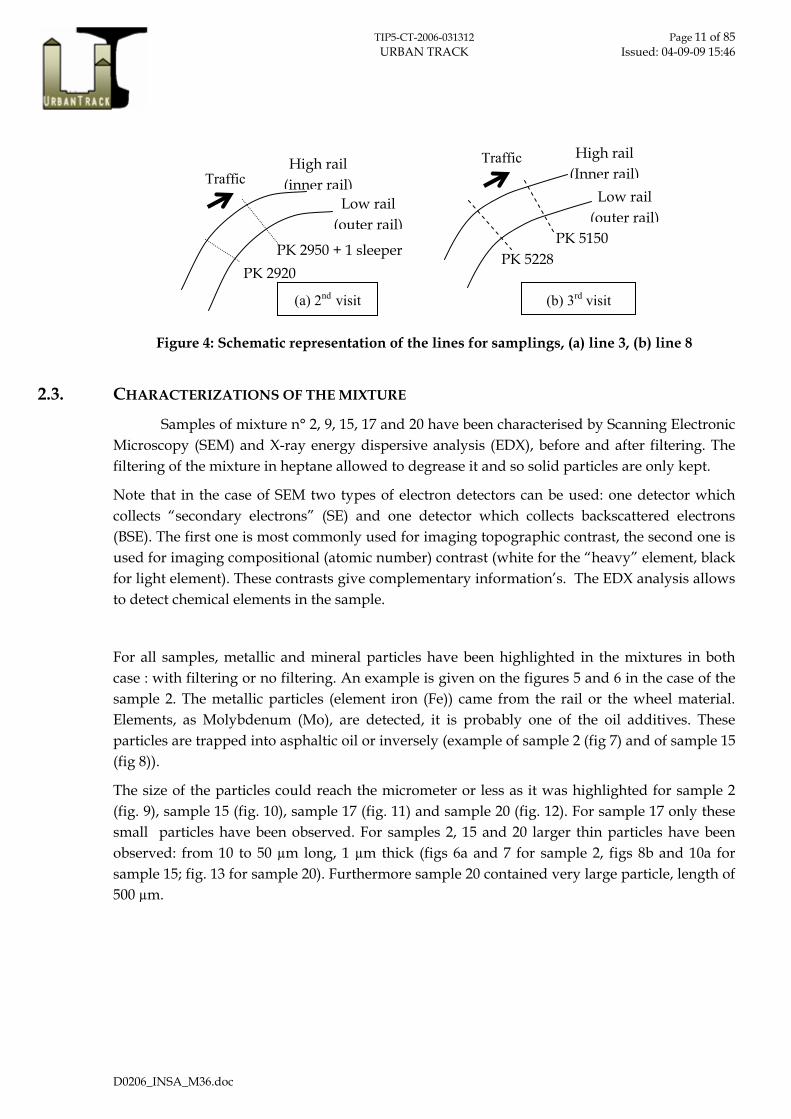
2.3. CHARACTERIZATIONS OF THE MIXTURE Samples of mixture n° 2, 9, 15, 17 and 20 have been characterised by Scanning Electronic Microscopy (SEM) and X-ray energy dispersive analysis (EDX), before and after filtering. The filtering of the mixture in heptane allowed to degrease it and so solid particles are only kept.
Note that in the case of SEM two types of electron detectors can be used: one detector which collects “secondary electrons” (SE) and one detector which collects backscattered electrons (BSE). The first one is most commonly used for imaging topographic contrast, the second one is used for imaging compositional (atomic number) contrast (white for the “heavy” element, black for light element). These contrasts give complementary information’s. The EDX analysis allows to detect chemical elements in the sample.
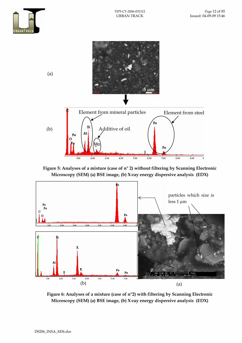
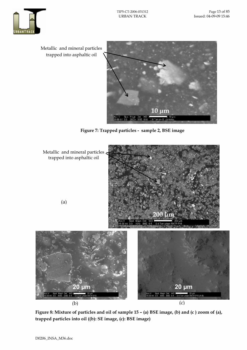
For all samples, metallic and mineral particles have been highlighted in the mixtures in both case : with filtering or no filtering. An example is given on the figures 5 and 6 in the case of the sample 2. The metallic particles (element iron (Fe)) came from the rail or the wheel material. Elements, as Molybdenum (Mo), are detected, it is probably one of the oil additives. These particles are trapped into asphaltic oil or inversely (example of sample 2 (fig 7) and of sample 15 (fig 8)).
The size of the particles could reach the micrometer or less as it was highlighted for sample 2 (fig. 9), sample 15 (fig. 10), sample 17 (fig. 11) and sample 20 (fig. 12). For sample 17 only these small particles have been observed. For samples 2, 15 and 20 larger thin particles have been observed: from 10 to 50 µm long, 1 µm thick (figs 6a and 7 for sample 2, figs 8b and 10a for sample 15; fig. 13 for sample 20). Furthermore sample 20 contained very large particle, length of 500 µm.
PK 2920 PK 2950 + 1 sleeper
High rail (inner rail)
(a) 2nd visit (b) 3rd visit
PK 5228PK 5150
TrafficTraffic
High rail (Inner rail)
Low rail (outer rail)
Low rail (outer rail)
TIP5-CT-2006-031312 Page 12 of 85 URBAN TRACK Issued: 04-09-09 15:46
D0206_INSA_M36.doc
Figure 5: Analyses of a mixture (case of n° 2) without filtering by Scanning Electronic Microscopy (SEM) (a) BSE image, (b) X-ray energy dispersive analysis (EDX)
Figure 6: Analyses of a mixture (case of n°2) with filtering by Scanning Electronic Microscopy (SEM) (a) BSE image, (b) X-ray energy dispersive analysis (EDX)
Element from mineral particles Element from steel
Additive of oil
Mo
(b)
5 µm
(a)
(b) (a)
particles which size is less 1 µm
TIP5-CT-2006-031312 Page 13 of 85 URBAN TRACK Issued: 04-09-09 15:46
D0206_INSA_M36.doc
Figure 7: Trapped particles - sample 2, BSE image
Figure 8: Mixture of particles and oil of sample 15 – (a) BSE image, (b) and (c ) zoom of (a), trapped particles into oil ((b): SE image, (c): BSE image)
200 µm
Metallic and mineral particles trapped into asphaltic oil
(a)
(b)
20 µm 20 µm
(c)
Metallic and mineral particles trapped into asphaltic oil
10 µm

TIP5-CT-2006-031312 Page 14 of 85 URBAN TRACK Issued: 04-09-09 15:46
D0206_INSA_M36.doc
Figure 9: Size of particles of Sample 2 – BSE image
(a) (b)
Figure 10: Size of particles of Sample 15 – (a) BSE image, (b) zoom of (a)
(a) (b)
Figure 11: Size of particles of sample 17 – (a) BSE image (b) zoom of (a)
2 µm 50 µm
50 µm 10 µm

TIP5-CT-2006-031312 Page 15 of 85 URBAN TRACK Issued: 04-09-09 15:46
D0206_INSA_M36.doc
Figure 12: Size of particles of sample 20
(a) (b)
Figure 13: Mixture of particles and oil of sample 20 – (a) SE image, (b) BSE image
Synthesis
Whatever the sample:
- metallic and mineral particles have been highlighted in the mixtures,
- these particles are trapped into the lubricant oil,
- the size of the particles reaches the micrometer or less.
For few samples large thin particles have been observed: from 10 to 50 µm long, 1 µm thick. But no conclusion could be drawn between this size and the localization of sample on the rail.
10 µm

TIP5-CT-2006-031312 Page 16 of 85 URBAN TRACK Issued: 04-09-09 15:46
D0206_INSA_M36.doc
3. MIXTURE RHEOLOGY In the aim to perform the study within moderate time and with moderate costs, while reproducing stresses conditions of the mixtures as close as possible as the ones found in real contact, two kind of tests are used (fig. 10):
- the Bridgman simulator, to characterize the rheology of the mixture “ex situ” (outside the rail-wheel contact). So the detachment of particles from the wheels and the rail is not taken into account,
- the “PeDeBa” simulator, to investigate the formation of the mixture and its range of action: rheology “in situ” is studied. So the detachment of particles is in this case taken into account and studied.
The tests reproduce conditions that are close to the ones found under contacts, i.e. high shearing and pressure conditions.
(a)
R
P0
mixture
Compression+torsion~ shear gradient under pressure
Ex situ
Local contact conditions are imposed and controlled
“Wheel” specimen
“Rail” specimen
In situ
(b)
Contact conditions nearest the reality
At
Ac
Figure 14: Schematic principle of the two kind of tests in laboratory, (a) Bridgman simulator, (b) “PeDeBa” simulator
3.1. TESTS ON THE “BRIDGMAN” SIMULATOR
3.1.1. Description
The rheology measurements of the mixture under high stresses (compression with a normal pressure P0 coupled with shear) were carried out on the "Bridgman" simulator with a geometry plan-plan.
The active part of the set-up (fig. 14a) is composed of:
- two cylindrical anvils Ac, of 6mm diameter, free to move vertically but fixed in rotation to apply the pressure P0 ,
TIP5-CT-2006-031312 Page 17 of 85 URBAN TRACK Issued: 04-09-09 15:46
D0206_INSA_M36.doc
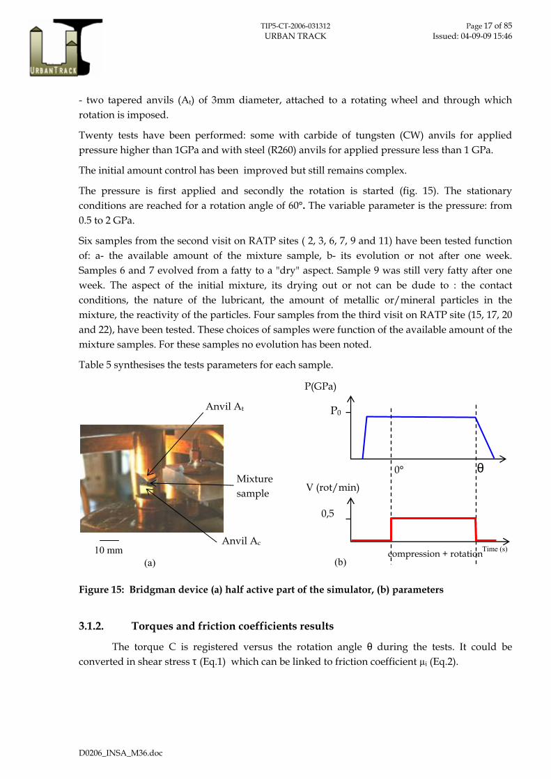
- two tapered anvils (At) of 3mm diameter, attached to a rotating wheel and through which rotation is imposed.
Twenty tests have been performed: some with carbide of tungsten (CW) anvils for applied pressure higher than 1GPa and with steel (R260) anvils for applied pressure less than 1 GPa.
The initial amount control has been improved but still remains complex.
The pressure is first applied and secondly the rotation is started (fig. 15). The stationary conditions are reached for a rotation angle of 60°. The variable parameter is the pressure: from 0.5 to 2 GPa.
Six samples from the second visit on RATP sites ( 2, 3, 6, 7, 9 and 11) have been tested function of: a- the available amount of the mixture sample, b- its evolution or not after one week. Samples 6 and 7 evolved from a fatty to a "dry" aspect. Sample 9 was still very fatty after one week. The aspect of the initial mixture, its drying out or not can be dude to : the contact conditions, the nature of the lubricant, the amount of metallic or/mineral particles in the mixture, the reactivity of the particles. Four samples from the third visit on RATP site (15, 17, 20 and 22), have been tested. These choices of samples were function of the available amount of the mixture samples. For these samples no evolution has been noted.
Table 5 synthesises the tests parameters for each sample.
Figure 15: Bridgman device (a) half active part of the simulator, (b) parameters
3.1.2. Torques and friction coefficients results
The torque C is registered versus the rotation angle θ during the tests. It could be converted in shear stress τ (Eq.1) which can be linked to friction coefficient µi (Eq.2).
(a)
Anvil At
Anvil Ac
Mixture sample
10 mm
P(GPa)
P0
V (rot/min)
compression + rotation
0° θ
0,5
(b) Time (s)

TIP5-CT-2006-031312 Page 18 of 85 URBAN TRACK Issued: 04-09-09 15:46
D0206_INSA_M36.doc
( ) 34 / 3C
Rτ =
Π
Eq. 1
0iµ
Pτ=
Eq. 2
Samples from the second visit (May 2007, line 3)
Parameters Results
Location
Samples Section fillet
Active flange
Non active flange
P0(GPa) θ (°)
Anvils Shear stress
τ (MPa) µi
2 X 0.5 CW 3.4 0,007
2 X 2 CW 17.6 0,009
3 X 0.5 CW 3.2 0,006
9 X 1 CW 9.5 0,009
7 X 0.5 CW 3.2 0,006
7 X 1 CW 6.0 0,006
6 X 1 CW 5.0 0.005
11 X 2 CW 12.8 0.006
Samples from the third visit (Nov. 2007, line 8)
Parameters Results
Location Samples
Section fillet Active flange
P0
(GPa) θ (°) Anvils
Shear stress
τ (MPa) µi
15 X 0.5 120 Steel 3.8 0,008
15 X 0.5 60 Steel 3.1 0,006
15 X 1 60 Steel 10.2 0,010
15 X 0.5 60 CW 3.3 0,007
17 X 0.5 60 CW 2.9 0,006
20 X 0.5 60 CW 2.5 0,005
22 X 0.5 180 Steel 6.2 0,012
22 X 0.5 60 Steel 8.4 0,017
22 X 1 60 Steel 14.6 0,015
Table 5: Parameters and results of the tests

TIP5-CT-2006-031312 Page 19 of 85 URBAN TRACK Issued: 04-09-09 15:46
D0206_INSA_M36.doc
The repeatability of the tests is good. The torque evolves in the same way for the same tests parameters (fig. 16). One can also note no difference in the case of steel or CW anvils.
0
0,5
1
1,5
2
0 10 20 30 40 50 60Rotation angle (°)
Torq
ue (N
.m)
P15 E2 0.5GPa
P15 E4 0.5GPa
P15 E7 0.5GPaCW
stee
stee
Figure 16: Repeatability of the tests – ex with sample 15 at 0.5GPa
For a same mixture torque increases with pressure (fig. 17). Consequently the shear stresses increase with pressure (table 5).
0
0,5
1
1,5
2
0 20 40 60
Rotation angle (°)
Torq
ue (N
.m)
P15 E2 0.5GPa
P15 E6 1GPa
P15 E4 0.5GPa
P15 E7 0.5GPa
0
0,5
1
1,5
2
0 20 40 60
Rotation angle (°)
Torq
ue (N
.m)
P17 E8 0.5GPa
(a) (b)
0
0,5
1
1,5
2
0 20 40 60
Rotation angle (°)
Torq
ue (N
.m)
P20 E9 0.5GPa
0
0,5
1
1,5
2
0 20 40 60Rotation angle (°)
Torq
ue (N
.m)
P22 E30.5GPaP22 E51GPa
(c ) (d)
Figure 17: Torque results, (a) Sample 15, (b) Sample 17, (c) Sample 20, (d) Sample 22
TIP5-CT-2006-031312 Page 20 of 85 URBAN TRACK Issued: 04-09-09 15:46
D0206_INSA_M36.doc
Friction coefficients µi (table 5) are very low.
In the case of the samplings on line 3 µi are inferior to 0.01 whatever the mixture is, in the range of the tested pressures.
In the case of the samplings on line 8 µi are inferior to 0.015 whatever the mixture is, in the range of the tested pressures. A very slight difference of behaviours of mixture of the fillet section and the one of the active flange has been observed. But this difference could not be stated positively because it is near the margin of error of the measurements.
3.1.3. Tribological analyses
The surface characterizations of the anvils after tests allow to determine the velocity accommodation location in the mixture. The surface are analysed by photonic microscopy and by Scanning Electronic Microscopy (SEM).
Observations of the anvils surfaces performed after tests with photonic microscope and SEM did not highlight any differences the different mixtures tested. The following observations presents the common morphologies that have been highlighted for all the tests.
Observations by photonic microscopy highlighted:
-“selective” ejection of parts of the mixture and fluid out of the contact,
- mixture, dried,
- oil bleeding from the mixture; the contact conditions causes the mixture to bleed the residue lubricant from its bulk. This oil-bleeding or migration formed like a fluid superficial layer at predominant layer of the mixture. This kind of phenomenon has been highlighted in previous work ([DESC05]),
- presence of surface complex (oil additives) on the surface of the mixture (shearing surface). This tends to prove that shearing, and so velocity accommodation, occurs « in » this surface,
-“trapping” of the additives of oil in the roughness of the anvil surface.
The figure 18 shows these different observations in the case of the sample 15 at 0.5GPa. The contact area is defined by the tapered anvil, so its diameter is 3 mm (dotted circular line on the figure 18).

TIP5-CT-2006-031312 Page 21 of 85 URBAN TRACK Issued: 04-09-09 15:46
D0206_INSA_M36.doc
Additives of the oil trapped into the anvil's scratches
(surfaces complex)
15 µm
(c)
"Dried" mixture
Oil bleedingSurfaces complex on the surface of the mixture (effects of oil additives)
(b)
200 µm
Ejected material out of the contact
Contact
(a)
2 mm
Figure 18: Images from optical microscopy (test with sample 15), (a) At surface, (b) and (c) Ac surface
After tests one re-found the elements constituted the initial mixtures: small metallic and mineral particles (figs 19b, 22c, 23b).
The presence of additives at the surface of the mixture and on the anvil surface chemical reaction of additives with surfaces anvils and with solid particles of the mixture. One detected in some areas a very thin film of oil at the extreme surface of the surface mixture (fig. 22b). The surfaces of the mixtures are smooth (figs 19a, 20, 22a). These different points highlight that sliding took place at the interface mixture/anvils surface during the tests. So the velocity accommodation occurred in the skin of the mixture, precisely in the surface complex (additives of the oil) and / or in a very thin film of fluid (formed because of the oil bleeding due to the high contact pressure). The velocity accommodation in the surface complex requires the formation of a smooth surface of the mixture’s skin.
Some small areas of the mixture surface show partial prints of the initial anvil Ac surface scratches (“replica”) (fig. 21). This highlights a partial adhesion of parts of the mixture to the anvil Ac during test. This also highlights that the local geometry (scale of µm) of the anvil surface (roughness…) is hidden by « trapping » the mixture and so a smooth surface is created, which then favoured a velocity accommodation in the skin of the mixture.
The figure 23 shows platelets constituted with different particles (mineral, metallic). So sliding took place between each platelet. Whereas this type of morphology is not the main one observed, it highlights shearing of the bulk of the mixture during the test. So the velocity accommodation occurred in the volume of the mixture. The velocity accommodation in the bulk of the mixture requires thus the formation of platelets constituted of particles detached from the wheels and the rail and agglomerated thanks to the initial lubricant.

TIP5-CT-2006-031312 Page 22 of 85 URBAN TRACK Issued: 04-09-09 15:46
D0206_INSA_M36.doc
Figure 19: Same area of At surface (test with sample 15), (a) topographic contrast image, (b) compositional contrast image
Figure 20: Topographic contrast images (test with sample 22) (a) surface of Ac, (b) surface of At
Anvil surface
Smooth surface of the mixture
Surface of the mixture
Smooth surface of the mixture
Smooth surface of the mixture Contact
Anvil

TIP5-CT-2006-031312 Page 23 of 85 URBAN TRACK Issued: 04-09-09 15:46
D0206_INSA_M36.doc
Figure 21: Topographic contrast image of surface mixture (Ac - test with sample 22)
(a)
(b) (c )
Figure 22: Mixture surface (At-test with sample 22), (a) topographic contrast image showing a smooth surface, (b) topographic contrast image, zoom of (a), (c) compositional contrast image of the same area of (b).
Thin film of oil at the interface mixture/anvil
Mixture = “oil” + particles
Very smooth agglomerates of mixture
Surface of the anvil
Prints of the anvils surface (Scratches): “replica” of the Ac
surface

TIP5-CT-2006-031312 Page 24 of 85 URBAN TRACK Issued: 04-09-09 15:46
D0206_INSA_M36.doc
Figure 23: Case of test with sample 22 - Same area of Ac surface, (a) topographic contrast image, (b) compositional contrast image
3.1.4. Synthesis
Friction coefficients are very low and are always inferior to 0.015 whatever the mixture is, in the range of the tested pressures (0.5-2GPa). Whether the materials of anvils are, in CW or in R260 steel, observations have highlighted:
oil bleeding from the mixture,
presence of surface complex (oil additives) on the surface of the mixture (shearing surface) and on the surface anvil. It highlights chemical reactions of additives with anvils surfaces and with the shearing surface of the mixture,
shearing of the bulk of the mixture and sliding at the interface mixture/anvils surface,
“selective” ejection of parts of the mixture out of the contact.
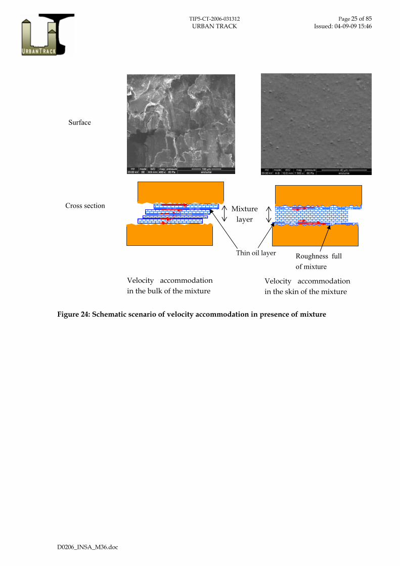
The velocity accommodation takes place either in the bulk of the mixture (shearing) or at the interface mixture/anvils surface (skin of the mixture, in the surface complex (additives)) (fig. 24). The additives (or surface complex) effect can be activated in the case of a very smooth surface which is induced by flows of the mixture. These flows fill in the roughness of the initial surface. Oil-bleeding modifies the limit conditions of the contact (µi). the velocity accommodation location modifies the detachment of particles (size, quantity…).
The torque, which is recorded during the tests, highlights that probably the oil-bleeding modifies the limit conditions (friction coefficient µi) of the contact.
Finally the tests highlight an equivalent behaviour of the mixtures collected on sites, at the scale of observations and in the range of the tested pressures.
Platelets Platelets constituted with different
particles (mineral, metallic)
TIP5-CT-2006-031312 Page 25 of 85 URBAN TRACK Issued: 04-09-09 15:46
D0206_INSA_M36.doc
Figure 24: Schematic scenario of velocity accommodation in presence of mixture
Mixture layer
Velocity accommodation in the skin of the mixture
Surface
Cross section
Velocity accommodation in the bulk of the mixture
Thin oil layer Roughness full of mixture

TIP5-CT-2006-031312 Page 26 of 85 URBAN TRACK Issued: 04-09-09 15:46
D0206_INSA_M36.doc
3.2. TESTS ON THE “PEDEBA” SIMULATOR
It allows to impose contact conditions nearest the reality of the wheel rail contact (formation of the mixture, pressure, slip,...). Its adaptation, to study the active flange rail lubrication, was completed and allows one more degree of freedom compared to the Bridgman simulator. Local contact conditions are also imposed and controlled precisely.
The aim of these tests is to understand the life cycle of the mixture in the wheel / rail active flange contact.
Experimentations on simulator were carried out to reproduce the active flange root contact. In order:
1- to impose contact conditions, especially the rolling / sliding that occurs on site,
2- to produce a mixture “as on site”,
3- to measure friction.
Tests on a “45° roller–plane” were carried out. Even these tests are not totally representative of reality, the results of tests are significant by comparing the morphologies of the surfaces obtained on site with those obtained on a simulator.
3.2.1. General experimental details
3.2.1.1. Progress of the tests Four series of tests have been carried out. - first series is a preliminary series, to determine the quantity, the initial location and the
best way to deposit the initial lubricant on the rail specimen. These preliminary tests also allowed to highlight the behaviour of the simulator in this configuration and to adjust the automatic controls.
- second and third series (series A and B), to study the tribological life of the mixtures and the corresponding evolution and value of the tangential force, with three different initial lubricants.
- fourth series (series C), to grasp mechanical conditions of run-off formation of the mixture on the rail, function of the slip rate and the lubricant.
For all the tests the lubricant is placed on the rail. It is easier rather than on the roller. Furthermore in the reality the lubricant is ejected from the injectors, to be placed on the rail.
3.2.1.2. The rolling contact simulator
The device (fig. 25) is composed of a lower assembly that applies normal force and an upper assembly that provides the rolling-sliding conditions. Normal force is applied by vertical hydraulic cylinders with force control. The forces are measured in three directions by a

TIP5-CT-2006-031312 Page 27 of 85 URBAN TRACK Issued: 04-09-09 15:46
D0206_INSA_M36.doc
piezoelectric sensor (longitudinal (Fx), lateral (Fy) and normal (Fz) forces). The upper assembly is composed of two guide columns and is guided in translation by hydrostatic bearings.
On the basis of this initial configuration, the longitudinal movement (Dx) of a rolling contact with partial or full sliding is obtained by installing a brushless motor on the table, the former being linked to a reduction gear that applies an angular speed proportional to the linear speed of the roller. The measurement of the angular speed is ensured by an incremental encoder. The torque applied by the motor, proportional to its current, is fully transmitted to the contact.
(a)
1 m
Rail
Roller
Loading zone
Rx 16
94 mm
rail specimen
roller
Loading zone (c)
(b)
Dx : displacement
Rail track
Figure 25: PeDeBa device
3.2.1.3. Specimen geometry determination
The dimensions of the specimens result from three compromises between:
• the possibilities of the simulator: normal load, the diameter of the rollers and the sliding parameter,
• the machining of the rail “flat” specimens in a sample of rail taken from a track after the passage of trains,
• the real geometries of the rails after rolling which means that the rail specimens are not really flat.

TIP5-CT-2006-031312 Page 28 of 85 URBAN TRACK Issued: 04-09-09 15:46
D0206_INSA_M36.doc
First it is possible to approximate the active flange – wheel contact in curve to an elliptic contact. The second hypothesis is that only one contact exists when negotiating the curve.
Such a contact can be simplified by a cone on a cylinder, representing contact conditions in curve with a tangent plane close to 45°. This avoids the experimental problems encountered when using conformal geometries. The contact area is elliptic. Then, taking into account the previous compromises, the geometry of both rail and wheel specimens and the applied normal load were determined by a numerical method (Finite element modelling, ABAQUS) to reach a contact pressure close to 3.5 GPa (Hertz contact pressure). Consequently, the roller has a radius of Rwx=16mm and a medium radius of R’wx=15mm (figs 26, 28). For the rail, first a bevelled edge was tooled along the length of the active flange of the rail specimen (fig. 27). Then this section was retooled to obtain a radius for the fillet section of the rail specimen of Rry=2mm (fig. 28).
Rwx = 16 mm
e = 10 mm
dint = 13 mm
Ra = 0,8 µm
Steel grade: ER7
Figure 26: Geometry of the roller
L = 114 mm
l = 14 mm
H = 25 mm
Rry =2mm
Ra = 0.8 µm
Steel grade = R260 (900 A)
Figure 27: Geometry of rail specimen
The rail specimen with a total length of 114 mm was fixed on the simulator with a precision of 5 µm to obtain a contact track whose width over a length of 30 mm did not vary more than 10%.
The parallelepiped-shaped test specimens are representing the rail. The rollers simulate behaviour of the wheel of a motorized axle. The wheel specimen (roller) and the rail specimen (rail) are sampled from respectively steel of a real wheel, and from the material composing the running surface of the rail. The surfaces of the rail specimen and the roller have no natural third
Rry
Rwx
e
Contact surface
Contact surface

TIP5-CT-2006-031312 Page 29 of 85 URBAN TRACK Issued: 04-09-09 15:46
D0206_INSA_M36.doc
body due to the differences in machining to obtain the geometry of the rail and wheel specimens.
Each rail specimen and roller are used to carry out two tests. Indeed, the length of the rail specimen enables carrying out two tests, i.e. two pathways, or two « running strips » of 30mm long.
Figure 28: Contact pressure and specimen geometry determination (a) contact is equivalent to a cylinder-plane contact, (b) Finite Element modelling, (c) elliptic contact
3.2.1.4. Friction coefficient calculation
This is calculated with the measured values of Fz, Fx and Fy:
Fz
Rry=2 mm
R’wx =15 mm
45°
1 2
Rwx=16 mm
12
3
Contact Pressure (MPa)
Contact area
Fz
Fy
FN
Fx
(a)
(b)
(c )

TIP5-CT-2006-031312 Page 30 of 85 URBAN TRACK Issued: 04-09-09 15:46
D0206_INSA_M36.doc
2 2
x xlongi
N z y
F FµF F F
= =+ (Eq. 3)
3.2.1.5. General kinematic data
The speed of the train (Vt) will be simulated by the linear speed of the rail specimen (Vl), itself determined by the displacement Dx and the frequency «f»,
Wheel rotation speed (Vr) is simulated by the rotation speed of the roller (Vg). The master-slave control of the simulator permits imposing the sliding, r, between the roller and the rail specimen (r= Vr / Vt =Vg / Vl) by taking into account the real radius of the roller when rolling which depends on the relative setting conditions of roller and the rail specimen. The absolute wheel slip (sliding of the roller), G, is expressed by r-1.
Control on slip regulation is obtained by applying the r quotient by accounting for the roller running radius so as to apply the roller speed, on the basis of the rail linear speed.
Classically the range of G is: 0 to 5% {[NICC02], [NICC05]}.
3.2.1.6. Testing progress
So as to stabilize roller / specimen in running-slip behaviour, each test will comprise several cycles for the same mechanical and kinematics conditions. Because of this, practical application of a complete cycle is split up into two phases (fig. 29a):
a half cycle for loading : Stages 1,2, 3,
a half cycle for unloading : Stages 3, 4, 1.
Each cycle starts at status 1, with initial roller configuration as compared to the rail, not loaded. Stages 1, 2, 3, and 4 make up a complete cycle. That implies that the running strip [a; b] of both the rail specimen and the roller is called upon x times, if x cycles are carried out for the same mechanical and kinematics condition.
Progress of a complete cycle comprises:
- stage 1-2: start of the half cycle for loading
Application of the normal load,
- stage 2-3: loading half cycle
Running and slip of the roller as compared to the rail. Distance [a; b] (fig. 29a) on the rail is constant, equal to the fixed travel. This distance is referred to as rail running strip. Distance [a; b] on the roller is constant. It constitutes the roller running strip,
- stage 3-4: end of half cycle for loading; start of half cycle for unloading
Stop of running, and slip and unloading,

TIP5-CT-2006-031312 Page 31 of 85 URBAN TRACK Issued: 04-09-09 15:46
D0206_INSA_M36.doc
- stage 4-1: unloading half cycle
Same as stage 2-3, but not loaded, and “running-slip” in the opposite direction.
The parameters applied are : Frequency (f), Displacement (Dx), Number of cycle (c), Normal load (Fz), Speed ratio (r).
During one test the recorded parameters :are the normal load Fz, the longitudinal force Fx (also classically named tangential force), the displacement. Figure 29b shows an example of the registered tangential force during 5 cycles.
Roller1
23
4
RAIL
b
ab
a
Fx
1 cycle Loading
Unloading
(a)
(b)
Figure 29: Progress of a complete cycle, (a) one complete cycle, (b) correlation with the Fx measurement
TIP5-CT-2006-031312 Page 32 of 85 URBAN TRACK Issued: 04-09-09 15:46
D0206_INSA_M36.doc
3.2.2. Preliminary tests
The aim of these 4 tests is to define a procedure to prepare and place the initial lubricant on the specimens. For the preliminary test, Vacuoline oil (commercial oil from Mobil) was used for the tests. This oil is used for the lubrication of the rails on the French urban rail network (RATP). Its kinematic viscosity is 150x10-6 m².s-1 at 40°C at atmospheric pressure (105 Pa).
3.2.2.1. Initial procedure
First a test has been carried out without lubricant – case of test 1909B1. Then lubrication tests with lubricant have been performed. The difficulty was to determine the quantity of lubricant to deposit on the rail specimen and its localization. Up to now the quantity of lubricant is not well known at RATP. But thanks to previous work with SNCF one knew approximately the quantity of lubricant placed on the rail by the injectors on SNCF network: 1.25 to 1.8 g/s. Considering the contact area for these tests compared to the real contact area, a mean quantity of lubricant of about 0,7 mg (i.e. 0,8.10-9 m3) can be estimated. On contrary the lubrication frequency is known: each 7 trains is a “lubricant train”. One train has 20 wheels (per rail). So “7 trains” fit with 7*20= 140 wheels passing. One cycle is equivalent to 1 wheel passing.
To test the incidence in modifying the quantity and the location of the initial lubricant on tangential force evolution (friction coefficient), three different initial distribution of the oil have been tested (table 6).
- 1 mg of oil is spread over the width of the rail and the length of rail track - case of test 1909A
- 0,2 mg of oil is deposited at the loading zone - case of test 1909B2
- a quantity of oil inferior to 0.05 mg is deposited respectively at the loading zone and in the middle of the rail track length – Case of test 1910B
under the same mechanical and kinematics conditions for all the tests
The lubricant is placed by droplet method on the rail. It is easier rather than on the roller. Furthermore in the reality, on the RATP network, the lubricant is directly ejected from the on-board injectors to be deposited on the rail. It could be noted that at SNCF the lubricant is first deposited by the injectors on the wheel flange, then deposited on the rail by transfer.

TIP5-CT-2006-031312 Page 33 of 85 URBAN TRACK Issued: 04-09-09 15:46
D0206_INSA_M36.doc
Test n° N’
cycles
N * Lubricant Initial
quantity
Initial location of the oil
on the rail track
1909B1 20
20 No 0 mg Without
1909A 140 140 Yes 1 mg Spread on track
1909B2 140 160 Yes 0,2 mg Loading zone
1910B **
B2 to B12
140
20 /test
140
360
Yes
<0,05 mg
3 small droplets +
3 small droplets
-
Loading zone
Track center
* N=cumulated cycles
** This test has been carried on after 140 cycles: 11 tests more with N’=20 cycles/test (ie 1 train). So the number of cumulated
cycles is N=360 at the end.
Table 6: location and quantity of lubricant for the preliminary tests
3.2.2.2. Mechanical applied parameters
Contact pressure: 5 GPa
Length of the track 30 mm
Rail speed: 60 mm/s (~0,2 km/h)
Slip rate G: 1% ([NICC02], [NICC05])
Number of cycles on the track for each lubrication sequence: 140
These cycle numbers are chosen on the basis of on-site data (lubrication frequency).
3.2.2.3. Preliminary tests results
The evolutions of friction coefficients are shown on figure 30.
Test with no lubricant Test 1909B1
15 mm
Loading zone: displacement
30 mm
rail
rail
rail
rail

TIP5-CT-2006-031312 Page 34 of 85 URBAN TRACK Issued: 04-09-09 15:46
D0206_INSA_M36.doc
The friction coefficient reaches 0.15 after 15 cycles. Noted that the typical value on the running table in reality is estimated about 0.25. But no measurements of friction coefficient in the case of active flange rail/ wheel contact are available. So it is difficult to compare with reality. Another point is that only 20 cycles have been performed because the surfaces have been quickly worn during this test. Perhaps it is no sufficient to reach 0.3.
Tests with lubricant Test 1909A
The friction coefficient is at the beginning of the test about 0.02, and is stable around 0.02 during the test. It looks like that an “elasto-plasto-hydrodynamics” lubrication stage is reached. The observations of the surface highlighted a contact completely full of lubricant (fig. 32). But one can think that the additives of the oil play also a role as it has been highlighted during the Bridgman tests, with a friction coefficient two times lower than for this test. On the border small quantity of a black pasty liquid is observed. Lubrication is too important in this test. So in the next test (1909B2) the quantity of lubricant has been decreased and only the loading point is lubricated.
Test 1909B2
Initially the lubricant was at the loading zone. The Fx measurements (fig. 31) show that during one cycle, Fx is not stable. During the cycle 5 Fx is about 150N. This value evolves during the test. For example during the cycle n° 104, Fx is about 100N during the first ¾ of the cycle and increase to 200 N at the end of the cycle. This evolution leads to the hypothesis that the lubricant has migrated along the track progressively during the test. This is confirmed by the observations of the rail track and the roller at the end of the test. They highlight that oil is present on the ¾ of the rail length track and on the roller track (fig. 33). The lubricant has been transported by the roller and so has progressively migrated along the rail track. This last point is coherent with on-site tests [DESC06, DESC08] where the transport of the lubricant and mixture by the wheel have been highlighted on SNCF network.
Test 1910B
The quantity of oil is less than for the test 1909B2.
The friction coefficient is stable at 0.05. To test the stability of this value this test has been carried on after 140 cycles: 11 tests more with 20 cycles/test (ie 1 train). So the number of cumulated cycles is 360 at the end. At 360 cycles the friction coefficient is still about 0.05. The test has been stopped because it has been noted a slight increase of the tangential force during the last ten cycles.
The oil is “travelled” by transfer on the roller and is replaced on the rail track. The contact is so progressively lubricated. At the same time particles are detached from the specimens. At the end of the test observations highlighted oil and oil+particles in the contact, on all the length of

TIP5-CT-2006-031312 Page 35 of 85 URBAN TRACK Issued: 04-09-09 15:46
D0206_INSA_M36.doc
the track and the presence of a black pasty liquid on the borders of the track and at the unloading zone (fig. 34). The surface of the rail and rollers tracks are very smooth (fig. 34). It seems like that the black pasty liquid has been spread on the surface and has filled in the holes of the surface. This black pasty liquid is constituted of particles that have been detached from the rail specimen or from the wheel specimen.
(a) (b)
(c) (d)
Figure 30: Friction coefficient, (a) without lubricant, (b), (c), (d) with lubricant
0.25
0
0.25
0
0.25
0
0.1
0 Number of cycles
Number of cycles Number of cycles
Number of cycles
µi
µi
µi
µi
Test 1909B2 Test 1910B
Test 1909B1
Test 1909A

TIP5-CT-2006-031312 Page 36 of 85 URBAN TRACK Issued: 04-09-09 15:46
D0206_INSA_M36.doc
(a) (b)
(c ) (d)
Figure 31: Tangential force Fx recorded during the test n°1909B2, (a) from cycle 2 to 7, (b) from cycle 32 to 37, (c ) from cycle 102 to 107, (d) from cycle 137 to 142
Fx
(N)
Fx
(N)
Fx
(N)
Fx
(N)
0
00
0
-100
-100-100
-100
-200
-200-200
-200
« End of the track (unloading zone) »
“Beginning of the track”
Half loading cycle
Plateau

TIP5-CT-2006-031312 Page 37 of 85 URBAN TRACK Issued: 04-09-09 15:46
D0206_INSA_M36.doc
Figure 32: Test 1909A, specimens tracks
Contact zone
Black “pasty liquid”
(b) Roller track
Contact zone
Displacement direction
(a) Location on the rail track: ½ length
Oil
Oil

TIP5-CT-2006-031312 Page 38 of 85 URBAN TRACK Issued: 04-09-09 15:46
D0206_INSA_M36.doc
Figure 33: Test 1909B2, specimens tracks
(a) Rail track: ¾ length track
Black “pasty liquid” (particles + oil)
(b) Roller track
Oil
Contact zone
Contact zone
Black “pasty liquid” (particles + oil)

TIP5-CT-2006-031312 Page 39 of 85 URBAN TRACK Issued: 04-09-09 15:46
D0206_INSA_M36.doc
Figure 34: Test 1910B, Rail track, N’= 360
(a) Normal view - Location : ½ length rail track
Black “pasty liquid” (particles + oil)
Layer of mixture.
Smooth surface Black “pasty liquid” (particles + oil)
(b) « Low angle » view
(c ) Unloading zone
Unloading zone
Particles in the contact

TIP5-CT-2006-031312 Page 40 of 85 URBAN TRACK Issued: 04-09-09 15:46
D0206_INSA_M36.doc
3.2.2.4. Intermediary conclusion
During these tests the migration and the transport of the lubricant by the wheel specimen has been highlighted [DESC08]. A “pasty liquid” is quickly formed. The hypothesis is this liquid is constituted of particles (detached from the rail or wheel specimens) mixed with the initial lubricant.
But the quantity of the initial lubricant seems to be to high to get a mixture as the one observed on site but moreover to reproduce a relevant life duration of the mixture. Indeed after 140 cycles (eq. to 7 trains) and after 360 cycles (eq. to 18 trains) the friction coefficient is constant at 0.05. This is important to be able to investigate the lubrication frequency. Moreover the contact conditions (contact dynamics, pressure…) are probably more stable than in the reality. But only the quantity of lubricant was investigated.
Consequently a new procedure has been defined to place less quantity of lubricant. In the same time a good repeatability of the deposit should be obtained.
3.2.3. Study of the tribological life of mixtures
Three series of tests have been carried out: series A, B and C. Series A and B allow to study the tribological life of the mixtures and the corresponding evolution and value of the tangential force, with three different initial lubricants. Series C allows to grasp mechanical conditions of run-off formation of the mixture on the rail, function of the slip rate and the lubricant.
3.2.3.1. New procedure for lubricant application
The samples were “cleaned” mechanically by ultrasound and chemically in an ethyl acetate bath for 5 minutes. This cleaning eliminated residual pollution due to specimen handling and machining (lubricant, particles) [DESC05]. Then rinsing was done in an ethanol bath for 5 minutes.
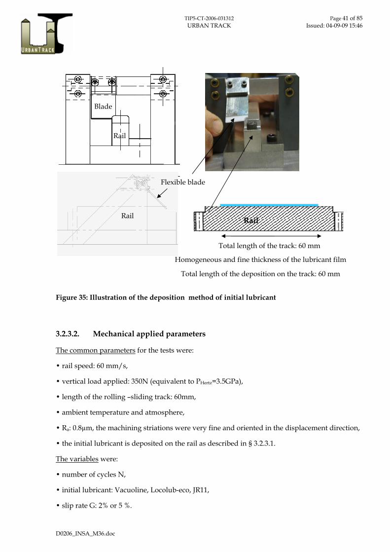
A droplet of oil of about 0.1 mg was first deposited at the loading zone and then spread over the width of the rail sample fillet and the length of rail track by a flexible polymer blade (fig. 35). Consequently, a homogeneous, fine layer of lubricant film was formed. Although it is not possible to easily quantify the thickness, this was the only way to reproduce as well as possible the same lubricant film (homogeneity and thickness).
TIP5-CT-2006-031312 Page 41 of 85 URBAN TRACK Issued: 04-09-09 15:46
D0206_INSA_M36.doc
Figure 35: Illustration of the deposition method of initial lubricant
3.2.3.2. Mechanical applied parameters
The common parameters for the tests were:
• rail speed: 60 mm/s,
• vertical load applied: 350N (equivalent to PHertz=3.5GPa),
• length of the rolling –sliding track: 60mm,
• ambient temperature and atmosphere,
• Ra: 0.8µm, the machining striations were very fine and oriented in the displacement direction,
• the initial lubricant is deposited on the rail as described in § 3.2.3.1.
The variables were:
• number of cycles N,
• initial lubricant: Vacuoline, Locolub-eco, JR11,
• slip rate G: 2% or 5 %.
Flexible blade
Rail
Total length of the track: 60 mm
Homogeneous and fine thickness of the lubricant film
Total length of the deposition on the track: 60 mm
Rail
Blade
Rail

TIP5-CT-2006-031312 Page 42 of 85 URBAN TRACK Issued: 04-09-09 15:46
D0206_INSA_M36.doc
The “Vacuoline” lubricant is used for the lubrication of the rails on the French urban rail network (RATP). The “Locolub-eco” is a biodegradable lubricant tested on the line 7bis of RATP network. “JR11” is a biodegradable lubricant provided by the society InS (Genay, France); this lubricant is not commercial. Vacuoline lubricant is chosen as the reference case.
The number of cycles was variable in the series A and B because :
- a stop criterion was chosen for tests 1945 to 1955: the tests were stopped when the apparent
friction coefficient µap , with xap
z
Fµ
F= , reached the value 0.3 one time along the contact length.
µap was used because it can be followed easily during all the test and along the contact length, contrary to µlongi.
- it allowed to follow the evolution of the mixture with the number of cycles (i.e. the number of wheels).
Series A
Test n° N Lubricant Load D - f V (mm/s) G %
1945 164 Vacuoline 0-350 60mm - 0,5 Hz 60 2
1946 93 Locolub-eco 0-350 60mm - 0,5 Hz 60 2
1948 240 JR 11 0-350 60mm - 0,5 Hz 60 2
Series B
Test n° N Lubricant Load D - f V (mm/s) G %
1949 980 Vacuoline 0-350 30mm - 1Hz 60 2
1950 4503 Vacuoline 0-350 60mm - 0,5 Hz 60 2
1951 400 Vacuoline 0-350 60mm - 0,5 Hz 60 2
1952 136 JR11 0-350 60mm - 0,5 Hz 60 2
1953 307 JR11 0-350 60mm - 0,5 Hz 60 2
1954 1002 Vacuoline 0-350 60mm - 0,5 Hz 60 2
1955 43 sans 0-350 60mm - 0,5 Hz 60 2
1956 980+1800+1600 Vacuoline 0-350 60mm - 0,5 Hz 60 2
1957 75 Vacuoline 0-350 60mm - 0,5 Hz 60 2
1958 80 JR 11 0-350 60mm - 0,5 Hz 60 2

TIP5-CT-2006-031312 Page 43 of 85 URBAN TRACK Issued: 04-09-09 15:46
D0206_INSA_M36.doc
Series C
Test n° N cycles Lubricant Load D - f V (mm/s) G %
1977A 200 Vacuoline 0-350 60mm - 0,5 Hz 60 2
1978 200 Vacuoline 0-350 60mm - 0,5 Hz 60 2
1979 60 Vacuoline 0-350 60mm - 0,5 Hz 60 2
1980 60 Vacuoline 0-350 60mm - 0,5 Hz 60 5
1981 60 Locolub-eco 0-350 60mm - 0,5 Hz 60 2
1982 60 JR11 0-350 60mm - 0,5 Hz 60 2
Table 7: Parameters of the tests
Figure 36 shows the evolution of the longitudinal friction coefficient µlongi (calculated via eq (3)) as a function of the number of cycles and the displacement Dx. Dx is null at the loading zone and equal to 60 mm (total contact length) at the unloading load. The small oscillations observed on the friction curve during one cycle can be explained by the passage of the balls of the ball bearing (roller support). This passage is visible due to the very high pressure imposed. That also highlights the great sensibility of the measurements.
Figure 36: Illustration of the evolution of the longitudinal friction coefficient µlongi
3.2.3.3. Repeatability of the tests
The friction coefficient evolves globally in the same way for the same tests parameters. (fig. 37). But at exactly the same number of cycles the value of friction coefficient can be different. On
Dx
µlongi
Contact length (mm)
Cycle number
TIP5-CT-2006-031312 Page 44 of 85 URBAN TRACK Issued: 04-09-09 15:46
D0206_INSA_M36.doc
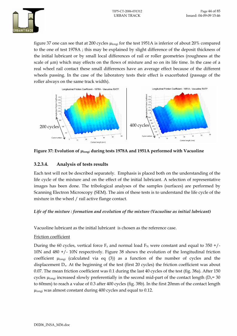
figure 37 one can see that at 200 cycles µlongi for the test 1951A is inferior of about 20% compared to the one of test 1978A ; this may be explained by slight difference of the deposit thickness of the initial lubricant or by small local differences of rail or roller geometries (roughness at the scale of µm) which may effects on the flows of mixture and so on its life time. In the case of a real wheel rail contact these small differences have an average effect because of the different wheels passing. In the case of the laboratory tests their effect is exacerbated (passage of the roller always on the same track width).
Figure 37: Evolution of µlongi during tests 1978A and 1951A performed with Vacuoline
3.2.3.4. Analysis of tests results
Each test will not be described separately. Emphasis is placed both on the understanding of the life cycle of the mixture and on the effect of the initial lubricant. A selection of representative images has been done. The tribological analyses of the samples (surfaces) are performed by Scanning Electron Microscopy (SEM). The aim of these tests is to understand the life cycle of the mixture in the wheel / rail active flange contact.
Life of the mixture : formation and evolution of the mixture (Vacuoline as initial lubricant)
Vacuoline lubricant as the initial lubricant is chosen as the reference case.
Friction coefficient
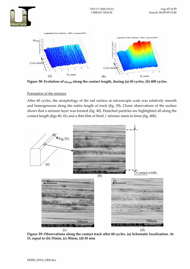
During the 60 cycles, vertical force Fz and normal load FN were constant and equal to 350 +/- 10N and 480 +/- 10N respectively. Figure 38 shows the evolution of the longitudinal friction coefficient µlongi (calculated via eq (3)) as a function of the number of cycles and the displacement Dx. At the beginning of the test (first 20 cycles) the friction coefficient was about 0.07. The mean friction coefficient was 0.1 during the last 40 cycles of the test (fig. 38a). After 150 cycles µlongi increased slowly preferentially in the second mid-part of the contact length (Dx= 30 to 60mm) to reach a value of 0.3 after 400 cycles (fig. 38b). In the first 20mm of the contact length µlongi was almost constant during 400 cycles and equal to 0.12.
200 cycles 400 cycles
TIP5-CT-2006-031312 Page 45 of 85 URBAN TRACK Issued: 04-09-09 15:46
D0206_INSA_M36.doc
Figure 38: Evolution of µlongi along the contact length, during (a) 60 cycles, (b) 400 cycles.
Formation of the mixture
After 60 cycles, the morphology of the rail surface at microscopic scale was relatively smooth and homogeneous along the entire length of track (fig. 39). Closer observations of the surface shows that a mixture layer was formed (fig. 40). Detached particles are highlighted all along the contact length (figs 40, 41) and a thin film of fluid / mixture starts to form (fig. 40b).
Figure 39: Observations along the contact track after 60 cycles. (a) Schematic localization. At Dx equal to (b) 15mm, (c) 30mm, (d) 45 mm
Dx (mm) Dx (mm)
µlongi
Cycle number
Cycle number
(b) (a)
(b)
(c) (d)
Fig.37c
(a) 500µm
Contact width
Dx Dx
500µm 500µm

TIP5-CT-2006-031312 Page 46 of 85 URBAN TRACK Issued: 04-09-09 15:46
D0206_INSA_M36.doc
Figure 40: Formation of a thin film of mixture after 60 cycles, at Dx equal to (a) 15 mm, (b) 30 mm, (c) zoom of (a)
Figure 41: Detachment of particles
Evolution of the mixture
After 400 cycles at microscopic scale, the morphology of the surface is not similar along the entire track.
In the first mid-part of the contact length (Dx = 0 to 25 mm), the width of the contact appears smooth (fig. 42a) and an accumulation zone can be seen on the borders of the track. Closer observations of the surface highlighted two different zones:
- a zone A[20mm] with a smooth surface similar to that observed after 60 cycles and containing both large particles and oil (fig. 42b), but not well mixed,
- a zone B[20mm] with a mixture (fig. 42c) containing a high quantity of small particles (mainly of micrometric size) mixed with liquid (fig. 42d).
Thin film of fluid
20 µm
Detached particles
Formation of a mixture
(a) (b)
(c)
50µm 50µm
Dx
Smooth surface
Detachment of particles or/and detached particles
Smooth surface
20µm
Dx

TIP5-CT-2006-031312 Page 47 of 85 URBAN TRACK Issued: 04-09-09 15:46
D0206_INSA_M36.doc
These morphologies are specific to low friction coefficient zones.
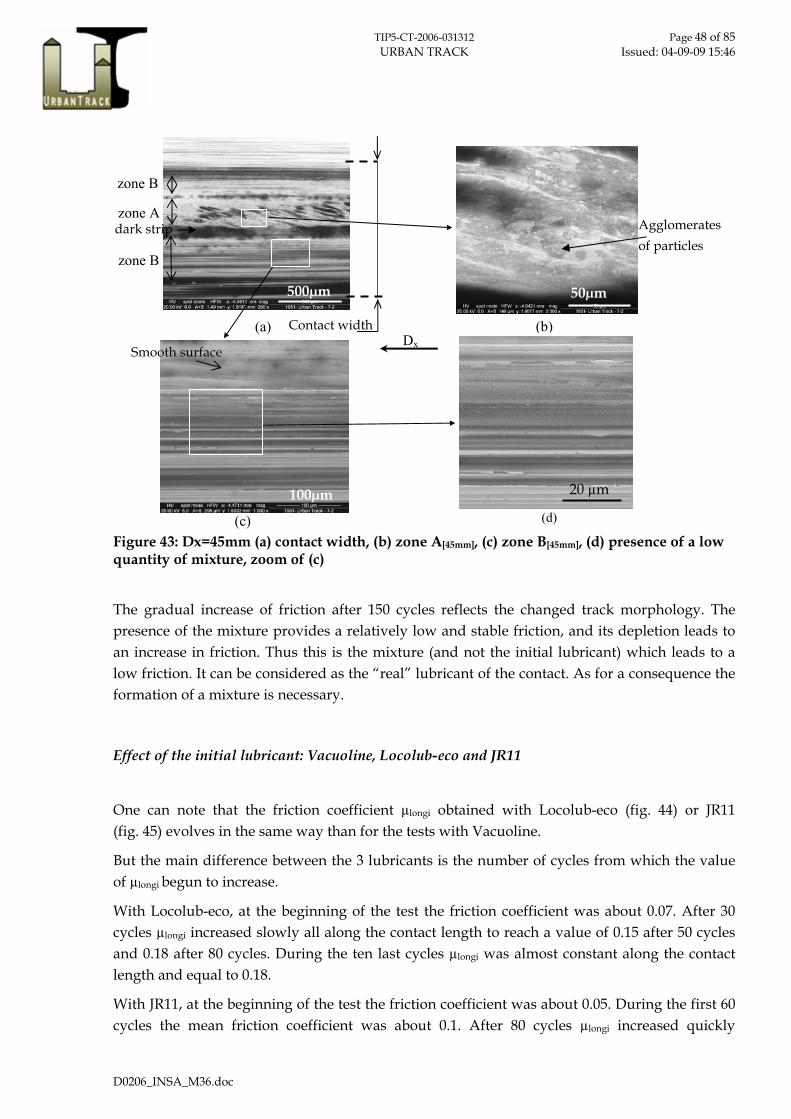
In the second mid-part of the contact length (Dx = 30 to 55 mm), the width of the contact has a different aspect (fig. 43a). Mixture accumulation zones remain on the borders of the track but the morphology observed in zones A and B is different:
- the surface of zone A[45mm] has a non smooth, dry aspect with agglomerates of particles and little or no liquid (fig. 43b). The liquid could have been ejected outside the contact or absorbed by the third body layer (“porous layer”) formed below during the first 100 cycles. A narrow band with a smooth surface remains.
- zone B[45mm] shows the presence of a mixture (fig. 43c) though in very low quantity compared to that of zone B[20mm] (fig. 43d).
Between zone A and B one can note a dark strip, which highlights a highest quantity of fluid than in brighter strips.
These morphologies are characteristic of a high friction coefficient (about 0.3).
Figure 42: Dx=20 mm, (a) contact width, (b) zone A[20mm] , (c) zone B[20mm], (d) zone full of mixture, zoom of (c)
Accumulation zone
Accumulation zone
(a)
(d) (c)
(b) Large particles Contact width
500µm 100µm
100µm 20µm
Dx
zone A
zone B
zone B
TIP5-CT-2006-031312 Page 48 of 85 URBAN TRACK Issued: 04-09-09 15:46
D0206_INSA_M36.doc
Figure 43: Dx=45mm (a) contact width, (b) zone A[45mm], (c) zone B[45mm], (d) presence of a low quantity of mixture, zoom of (c)
The gradual increase of friction after 150 cycles reflects the changed track morphology. The presence of the mixture provides a relatively low and stable friction, and its depletion leads to an increase in friction. Thus this is the mixture (and not the initial lubricant) which leads to a low friction. It can be considered as the “real” lubricant of the contact. As for a consequence the formation of a mixture is necessary.
Effect of the initial lubricant: Vacuoline, Locolub-eco and JR11
One can note that the friction coefficient µlongi obtained with Locolub-eco (fig. 44) or JR11 (fig. 45) evolves in the same way than for the tests with Vacuoline.
But the main difference between the 3 lubricants is the number of cycles from which the value of µlongi begun to increase.
With Locolub-eco, at the beginning of the test the friction coefficient was about 0.07. After 30 cycles µlongi increased slowly all along the contact length to reach a value of 0.15 after 50 cycles and 0.18 after 80 cycles. During the ten last cycles µlongi was almost constant along the contact length and equal to 0.18.
With JR11, at the beginning of the test the friction coefficient was about 0.05. During the first 60 cycles the mean friction coefficient was about 0.1. After 80 cycles µlongi increased quickly
20 µm
(d) (c)
(a) (b)
Smooth surface
Contact width
500µm 50µm
100µm
Dx
zone A
zone B
zone B
dark strip Agglomerates of particles

TIP5-CT-2006-031312 Page 49 of 85 URBAN TRACK Issued: 04-09-09 15:46
D0206_INSA_M36.doc
preferentially in the second mid-part of the contact length (Dx= 25 to 50mm) to reach a value of 0.3 after 120 cycles.
Figure 44: Initial lubricant Locolub-eco, Evolution of µlongi along the contact length, during the tests (a) 1981A and (b) 1946A
Figure 45: Initial lubricant JR11, Evolution of µlongi along the contact length, during the tests (a) 1982A and (b) 1952A
The morphology of the surface is similar along the entire track, in the two cases of lubricant Locolub eco or JR11, at microscopic scale. But as for Vacuoline lubricant, the width of the contact has different surface aspect, both for Locolub-eco (fig. 46a) and for JR11 (fig. 47a). Closer observations highlighted two different zones (zone A, zone B). The purpose is illustrated at Dx=30mm.
For Locolub-eco mixture accumulation zones remains on the borders of the track. Two different morphologies are observed in zones A and B:
- the surface of zone A[30mm] has a non smooth, dry aspect with agglomerates of particles and little or no liquid (fig. 46b). The quantity of these agglomerates is lower than for Vacuoline. As
80 cycles 50 cycles
µlongi µlongi
(b) (a)
30 cycles
µlongi
(a)
120 cycles
µlongi
(b)

TIP5-CT-2006-031312 Page 50 of 85 URBAN TRACK Issued: 04-09-09 15:46
D0206_INSA_M36.doc
for Vacuoline the liquid could have been ejected outside the contact or absorbed by the third body layer (“porous layer”) formed below during the first 30 cycles.
- the zone B[30mm] has a smooth surface and a band with a high quantity of liquid (dark on fig. 46c). This zone contains both small detached particles and oil, but not well mixed (fig. 46d). The quantity of particles is lower then the one observed in the zone B of the test with Vacuoline (fig. 43d).
Between zone A and B one can note dark strips, which highlights a highest quantity of fluid than in brighter strips.
The zone A shows the same characteristics than the one highlighted in the case of test with Vacuoline and high friction coefficient. But the width of the zone A is smaller and contains less agglomerates. One assumes that this zone is in curse of formation. Its presence can explain the increase of µlongi.
For JR11, the mixture accumulation zones on the borders of the track are very large. Two different morphologies are observed in zones A and B:
- the surface of zone A[30mm] has a non smooth, dry aspect with agglomerates of particles and little or no liquid (fig. 47b). The quantity of these agglomerates is similar of the one for Vacuoline.
- the zone B[30mm] has a smooth surface (fig. 47c). This zone contains also a quite high quantity of detached particles. These particles have different sizes (fig. 47d) from the µm to about ten µm.
As for tests with Vacuoline or with Locolub-eco, a specific zone is present (zone A) characteristic of high friction coefficient.

TIP5-CT-2006-031312 Page 51 of 85 URBAN TRACK Issued: 04-09-09 15:46
D0206_INSA_M36.doc
Figure 46: Initial lubricant Locolub-eco, Dx=30 mm (a) contact width, (b) zone A[30mm], (c) zone B[30mm], (d) presence of a mixture
Figure 47: Initial lubricant JR11, Dx=30 mm, 150 cycles (a) contact width, (b) zone A[30mm], (c) zone B[30mm], (d) particles
Agglomerates of particles
20 µm
(d)
(a) (b)Smooth surface
Contact width
500µm 40µm
50µm
Dx
(c)
Accumulation zone
zone A zone B
zone B
(c)
30 µm
(d)
(a) (b)
Smooth surface
Contact width
500µm 50µm
100µm
Dx
(d)
Accumulation zone
zone A
zone B
zone B
dark strip
dark strip

TIP5-CT-2006-031312 Page 52 of 85 URBAN TRACK Issued: 04-09-09 15:46
D0206_INSA_M36.doc
During the tests performed with the three lubricants a mixture has been formed. The formation of the mixture is linked to the formation of a smooth surface. But, in the case of Locolub-eco and JR11, it seems difficult to form a homogeneous well mixed (fluid + particles) mixture, as it can be observed in the case of the Vacuoline (fig. 42d).
In the three cases of lubricants a given friction coefficient value can be correlated to the same given morphology that characterizes the localization of the mixture in the contact, specifically when the value is high (0.3) (table 8). When the friction coefficient increases one highlighted the formation (or the presence) of a band along the contact length (noted zone A). In this band agglomerates of particles are formed and the mixture became dry.
Lubricant N total
of cycles
Initial morphology and
µlongi value
Final morphology and µlongi valueI
(along the track)
Formation of mixture
M cyclesII
Vacuoline 400
µlongi init= 0.07
µlongi final ~ 0.12
µlongi final ~ 0.30
150
Locolub-eco
93
µlongi init= 0.07
µlongi final ~ 0.18 30
JR11 136 µlongi init= 0.05
µlongi final ~ 0.15
µlongi final ~ 0.3
60
Table 8 : Effect of the initial lubricant - Synthesis
I Two different values of µlongi can be measured during 1 cycle along the contact length. II M = number of cylces during which a steady state is obtained (the value of µlongi is constant and about 0.1). After M
cycles, the value of µlongi begun to increase.
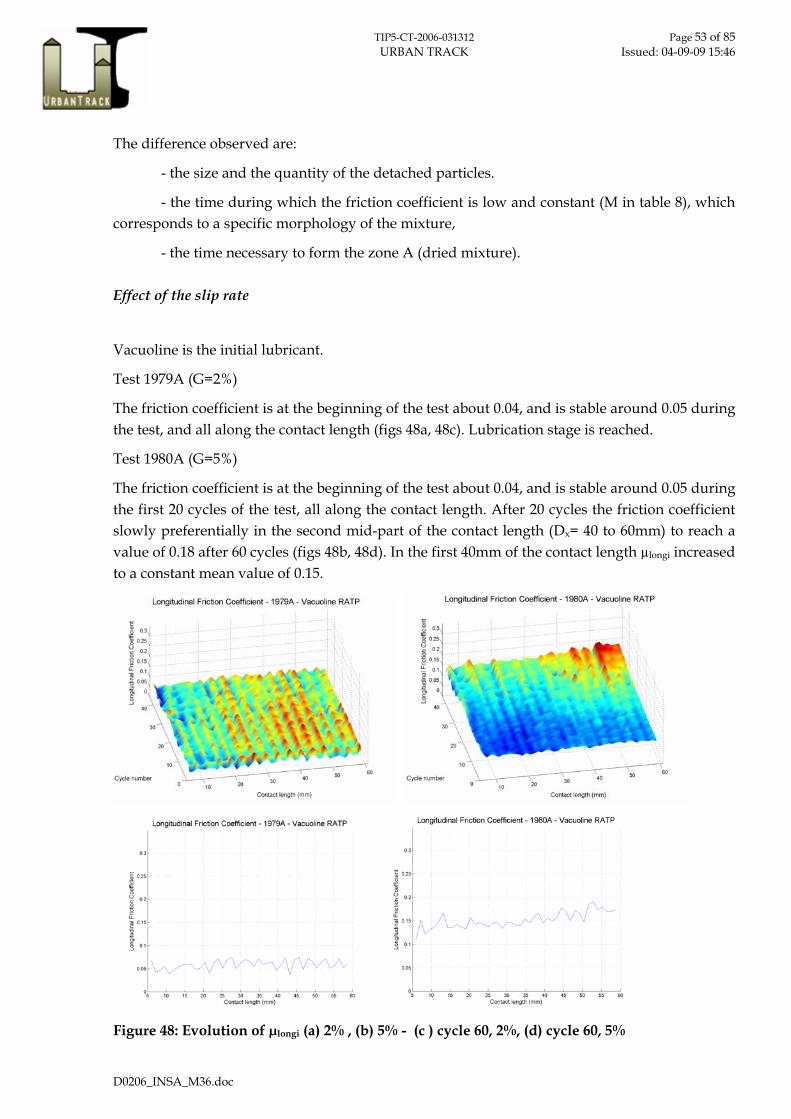
TIP5-CT-2006-031312 Page 53 of 85 URBAN TRACK Issued: 04-09-09 15:46
D0206_INSA_M36.doc
The difference observed are:
- the size and the quantity of the detached particles.
- the time during which the friction coefficient is low and constant (M in table 8), which corresponds to a specific morphology of the mixture,
- the time necessary to form the zone A (dried mixture).
Effect of the slip rate
Vacuoline is the initial lubricant.
Test 1979A (G=2%)
The friction coefficient is at the beginning of the test about 0.04, and is stable around 0.05 during the test, and all along the contact length (figs 48a, 48c). Lubrication stage is reached.
Test 1980A (G=5%)
The friction coefficient is at the beginning of the test about 0.04, and is stable around 0.05 during the first 20 cycles of the test, all along the contact length. After 20 cycles the friction coefficient slowly preferentially in the second mid-part of the contact length (Dx= 40 to 60mm) to reach a value of 0.18 after 60 cycles (figs 48b, 48d). In the first 40mm of the contact length µlongi increased to a constant mean value of 0.15.
Figure 48: Evolution of µlongi (a) 2% , (b) 5% - (c ) cycle 60, 2%, (d) cycle 60, 5%

TIP5-CT-2006-031312 Page 54 of 85 URBAN TRACK Issued: 04-09-09 15:46
D0206_INSA_M36.doc
Morphology of the tracks
After 60 cycles the thickness of the mixture is less important at 2% than at 5% of slip ratio (fig. 49). Agglomerates of particles are only present at 5% (figs 49, 50c, 50f). The figures 50a and 50d shows that dark strips (link to the quantity of fluid) are present in both case 2% and 5%, but at 2% these strips are wider than at 5% (figs 50a, 50d). More bright strips are observed at 5%.
There are a higher quantity of detached particles at 5% (figs 50b, 50e). One can note also that large particle are detached at 5% (fig. 50f).
At 2% the characteristic morphology of a low friction coefficient is observed.
At 5% the characteristic morphology of a high friction coefficient is in formation.
Figure 49: Track morphologies after 60 cycles – Photonic microscope images, (a), (c) G=2%, (b), (d) G=5%
(d) (c)
(b) (a)
Agglomerates Surface complex
Surface complex

TIP5-CT-2006-031312 Page 55 of 85 URBAN TRACK Issued: 04-09-09 15:46
D0206_INSA_M36.doc
Figure 50: Track morphologies after 60 cycles – SEM images, (a), (b), (c) G=2% , (d), (e), (f) G=5%
(c) (f)
(b)
(d)
Dark strip
Dark strip
500µm
50µm
20µm
50µm
500µm
(a)
Thin film of fluid or mixture
Smooth surface
Detached particles
30µm
(e)
Agglomerates
of particles
Detachment of a large particle
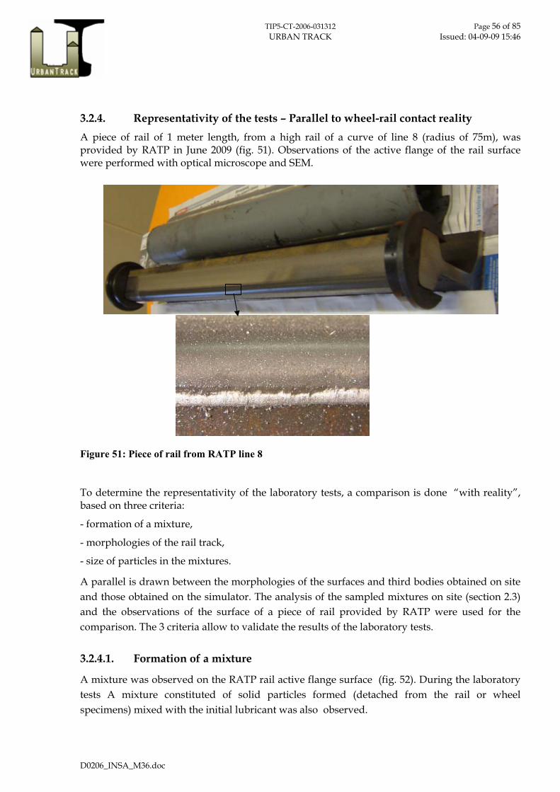
TIP5-CT-2006-031312 Page 56 of 85 URBAN TRACK Issued: 04-09-09 15:46
D0206_INSA_M36.doc
3.2.4. Representativity of the tests – Parallel to wheel-rail contact reality A piece of rail of 1 meter length, from a high rail of a curve of line 8 (radius of 75m), was provided by RATP in June 2009 (fig. 51). Observations of the active flange of the rail surface were performed with optical microscope and SEM.
Figure 51: Piece of rail from RATP line 8
To determine the representativity of the laboratory tests, a comparison is done “with reality”, based on three criteria:
- formation of a mixture,
- morphologies of the rail track,
- size of particles in the mixtures.
A parallel is drawn between the morphologies of the surfaces and third bodies obtained on site and those obtained on the simulator. The analysis of the sampled mixtures on site (section 2.3) and the observations of the surface of a piece of rail provided by RATP were used for the comparison. The 3 criteria allow to validate the results of the laboratory tests.
3.2.4.1. Formation of a mixture
A mixture was observed on the RATP rail active flange surface (fig. 52). During the laboratory tests A mixture constituted of solid particles formed (detached from the rail or wheel specimens) mixed with the initial lubricant was also observed.

TIP5-CT-2006-031312 Page 57 of 85 URBAN TRACK Issued: 04-09-09 15:46
D0206_INSA_M36.doc
Figure 52: RATP rail surface (active flange)
3.2.4.2. Track morphologies
The observations of RATP rail active flange surface highlighted a smooth surface and digitations (fig. 53). Similar morphologies were observed on rail specimens after laboratory tests.
3.2.4.3. Size of mixtures particles
The sizes of particles of the mixture, observed on real specimens and on tests specimens, have the same characteristic scale (fig. 54).
The size of the particles can reach a micrometer or less. Larger thin particles (“platelets”) from 10 to 50 µm long and about 1 µm thick were also observed.
Particles
Oil bleeding
(a) (b)
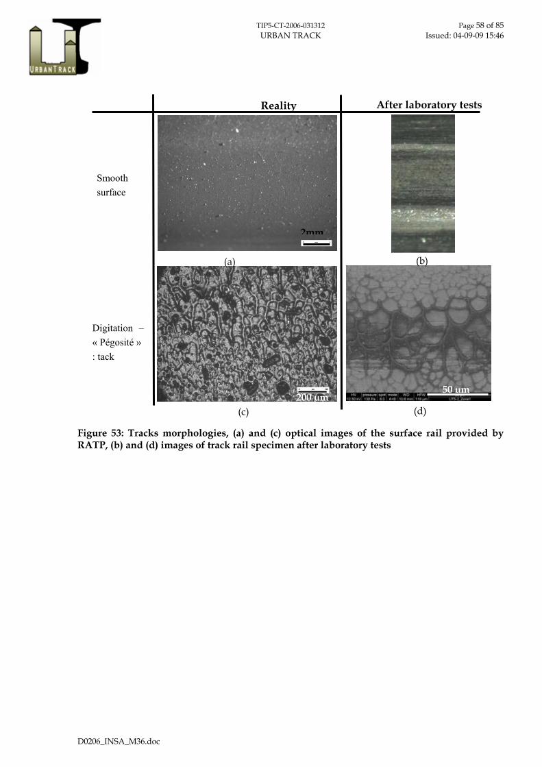
TIP5-CT-2006-031312 Page 58 of 85 URBAN TRACK Issued: 04-09-09 15:46
D0206_INSA_M36.doc
Figure 53: Tracks morphologies, (a) and (c) optical images of the surface rail provided by RATP, (b) and (d) images of track rail specimen after laboratory tests
Digitation – « Pégosité »: tack
50 µm200 µm
Smooth surface
After laboratory tests Reality
(a) (b)
(c) (d)
2mm

TIP5-CT-2006-031312 Page 59 of 85 URBAN TRACK Issued: 04-09-09 15:46
D0206_INSA_M36.doc
Figure 54: SE images (a) of the surface rail provided by RATP, (c) of the mixture sampled on site, (b) and (d) of the specimen rail surface with a mixture formed during laboratory tests
3.2.5. Synthesis
The validity of the laboratory tests was determined by comparison between the mixture sampled on-site and that formed during the tests.
The main advantages of such laboratory tests are, on the one hand, they permit the precise control of local contact conditions while, on the other hand, they can be performed inexpensively (compared to full scale tests or on-site tests). This enables repeating tests in order to reduce data scatter.
(a) (b)
(c) (d)
Reality After laboratory tests
« platelets »
10 µm
10 µm 10 µm
10 µm
TIP5-CT-2006-031312 Page 60 of 85 URBAN TRACK Issued: 04-09-09 15:46
D0206_INSA_M36.doc
The tests allow to discriminate the three lubricants in term of lifetime of the mixture formed with each of one. So it is now possible to investigate lubrication frequency.
And the functioning of new lubricants can be validate under realistic contact conditions in laboratory, easier than on site (“less dangerous, less time, lower costs”).
The tests reproduced conditions that were close to those found in wheel-rail contacts, i.e. high shearing ([1%-5%]) and pressure conditions (3.5 GPa). Under these controlled conditions the tests reproduced the formation of the mixture as it was observed on-site. A given friction coefficient value can be correlated to a given morphology that characterizes the localization of the mixture in the contact, whereas the relative quantity of oil and particles in the mixture, which probably determines its specific rheology, in turn defines the friction and wear of the wheel flange/rail gauge contact. This specific rheology is activated and more efficient with the smoothing of the surface. This last can be formed by the “trapping” and the filling in of the roughness (scale of µm) by the mixture itself (fig. 24).
In this phenomenological study, tracking the evolutions of morphologies permits establishing a preliminary scenario of how the mixture functions, whatever the initial lubricant.
In the case of a low friction coefficient, a smooth surface starts forming and particles (from the rail or wheel specimens) become detached. These particles mix with the lubricant, leading to the formation of a mixture whose properties allow it to flow easily in the contact. The contact conditions chosen for the test appear to lead to an efficient mixture.
In the case of a high friction coefficient, a dried mixture is highlighted.
This scenario, which partially validates the morphology of the mixture leading to a low friction coefficient during the tests, is comparable to that required for efficient lubrication on-site and described by experts in the field of wheel-rail contact lubrication.
The incidence of the initial lubricant is correlated first to its capacity to stay in the contact and to mix with the detached particles, then to its reactivity with the detached particles (role of the lubricant additives). The velocity accommodation location (bulk or skin of the mixture) effects on the quantity of detached particles and on their size, consequently effects on the relative quantity fluid/particles and on the reactivity fluid/solid particles.
Both initial lubricant and contact conditions determine the formation of the mixture and then determine the “good” rheology. This rheology, in the range of contact stresses, leads to the “good” location of velocity accommodation, and so to a low value of the friction coefficient and trapping of the mixture in the contact.

TIP5-CT-2006-031312 Page 61 of 85 URBAN TRACK Issued: 04-09-09 15:46
D0206_INSA_M36.doc
4. NUMERICAL INVESTIGATIONS ON LOCAL WHEEL-RAIL CONTACT CHARACTERISTICS
The aim of the present part is to access to local wheel-rail contact characteristics (i.e. contact positions on the rail surface, contact pressures and plastic deformations) under various lateral loading conditions from straight track to sharp curved track. The access to such characteristics will contribute to better understanding the local tribological observations previously made on site, i.e. localisation of contact zone and plastic deformations. The influence on these characteristics of new or worn profile and under or over lubrication will be evaluated.
Three main wheel-rail contact configurations are usually admitted for a wheel-rail couple which is new profile and could be schematically summed up as followed:
- the first is a mono-contact centred on the rolling table (fig. 55a). This configuration is observed on straight tracks or curves with wide radii.
- the second is a bi-contact (fig. 55b). On the rolling table, the contact zone slightly displaced toward the active flange. On the active flange, a second contact zone occurs. This configuration is observed on curves with a medium radii.
- The third is a mono-contact (fig. 55c). No contact remains on the rolling table, this last only occurs on the active flange. This configuration is observed on curves with a small radii.
Rolling table contact : friction coefficient µ j And active flange contact: friction coefficient µ k
Rolling table contact: friction coefficient µ i
Active flange con tact : friction coefficient µ l
(a)
(b)
(c )
Figure 55: Schematic main wheel-rail contact configurations
When lubrication is properly made, the friction coefficient changes on the rail surface along the transversal direction: around 0.3 on the top of the rolling table and around 0.01 (measured previously on Bridgman simulator) on the active flange.

TIP5-CT-2006-031312 Page 62 of 85 URBAN TRACK Issued: 04-09-09 15:46
D0206_INSA_M36.doc
If lubrication is not properly made, two cases could be discriminated: the first is the under-lubrication, the second is the over-lubrication. When under-lubrication occurs, the friction coefficient could reach the limit value of 0.3 all over the rolling table and the active flange: this case is equivalent to dry contact conditions. When over-lubrication occurs, the friction coefficient could reach the limit value of 0.01 all over the rolling table and the active flange. Of course, these two last cases are purely theoretical and are not observed on site… Nevertheless, these two extreme cases will be used to exacerbate the effect of lubrication (friction coefficient variation) on the contact characteristics… the lubrication reality, which would required a model with two friction coefficient on the rail surface (actual model doesn’t converge in this case, being nevertheless between this two extreme cases.
The present part will be split into 3 paragraphs:
- wheel-rail contact models and choices
- wheel-rail contact characteristics and parallel to reality
- influence of the friction coefficient, simulating under and over lubrication, on the wheel-rail contact characteristics
4.1. WHEEL-RAIL CONTACT MODELS AND CHOICES
Three wheel-rail contact models have been tested: from a classical 2D model to a more complex 3D model. Each model is based on the same principle which is presented figure 56. In order to estimate contact characteristics, a quasi-static finite element model has been developed with Abaqus 6.7.1 software.
WITH P: VERTICAL LOADING AND Q: LATERAL LOADING
Figure 56: Principle of the wheel-rail contact models

TIP5-CT-2006-031312 Page 63 of 85 URBAN TRACK Issued: 04-09-09 15:46
D0206_INSA_M36.doc
Wheel and rail profiles:
The wheel and rail profiles have been supplied by RATP: profiles of new wheel and new rail, and profiles of two worn wheels of MF77 that have circulated on line 8 and profiles of right and left rails that have been measured during the third visit on RATP site (line 8).
New wheel profile from RATP : V135.igs New rail profile from RATP: V52.igs Worn wheel profile from RATP : 13112002-profil nf-f 03-402 usé essieu 1 roue d.igs 13112002-profil nf-f 03-402 usé essieu 1 roue g.igs Worn rail profile from RATP : L8-Pk5150-V2-FE-08-11-07.igs
L8-Pk5150-V2-FI-08-11-07.igs Material:
The material used for both wheel and rail is equivalent to R260 steel. This bilinear plastic law has an elastic limit equal to 480 MPa and a plastic deformation of 2% at 900 MPa.
Global track stiffness:
The “global track stiffness” has been given by RATP and is equal to ktransv = 4.7 107 N/m along the transversal direction and kvert = 5 107 N/m along the vertical direction. These stiffness has been applied directly under the rail foot.
Loading conditions:
The loading are discomposed into two parts: - The vertical loading, called P, which is equivalent to the axle load: 90 kN for a MF77. - The lateral loading, called Q, which is equivalent to the centrifuge effect: from 0 kN on
perfect straight track to about 45 kN (half of the axle load) on sharp curved track.
Contact conditions:
For each model, the Lagrange multiplier method has been used to solve the contact problem: each wheel is a master surface and each rail a the slave surface. Friction coefficient remains constant both over the master/slave surfaces and during the simulations.
4.1.1. A classical 2D model of wheel-rail contact at full-scale
Based on the previously described characteristics, the classical 2D model of wheel-rail contact (fig. 57) is meshed with CPE4 elements (i.e. linear quadrangle with 4 nodes formulated in plain strain).

TIP5-CT-2006-031312 Page 64 of 85 URBAN TRACK Issued: 04-09-09 15:46
D0206_INSA_M36.doc
Figure 57: global view of the 2D mesh
The size of the elements in the refined zone (near the contact) is respectively for the rail 100 µm x 100 µm (slave surface) and for the wheel 300 µm x 300 µm (master surface), see figure 58.
The number of CPE4 elements is : - about 45 000 elements for each rail, - about 24 000 elements for the wheelset
The entire model contains about 114 000 elements
(a) (b) Figure 58: (a) local view of the 2D mesh of the new wheel-rail couple, (b) local view of the 2D
mesh of the worn wheel-rail couple The results obtained with such a model are presented figure 59-a. Once the vertical load P of 90 kN is applied, the lateral load Q is progressively applied from 0 kN to 45 kN. Initially, the contact occurs at the centre of the rail which is classical. The contact pressure is about 950 MPa as expected with Hertz theory in this case. While increasing the lateral load Q, the contact zone

TIP5-CT-2006-031312 Page 65 of 85 URBAN TRACK Issued: 04-09-09 15:46
D0206_INSA_M36.doc
displaced toward the active flange and the contact pressure increase as expected. Nevertheless, the displacement of the railhead ( on figure 58-a) reach the unrealistic value of 21.4 mm along the transversal direction (table 9), as compared to those obtained with a 3D model. The same thing occur for the Von Mises stress level which reaches values close to 5 GPa. As a consequence, a “classical 2D finite element model” could not be used to help understanding local wheel-rail contact conditions. As for a consequence, either an improvement of the actual 2D model or a natural 3D finite element model have now to be used. To save computation time, the 2D model will be first improved.
classical 2D model 2D with 3D stiffness 3D
Lateral railhead disp. 21.4 mm (error 229%) 6.55 mm (error >1%) 6.5 mm
Lateral wheel disp. 25.2 mm (error 105%) 10.5 mm (error 14%) 12.3 mm
Table 9: Comparison between the three models tested: “classical 2D model”, “2D with 3D stiffness” and “3D”
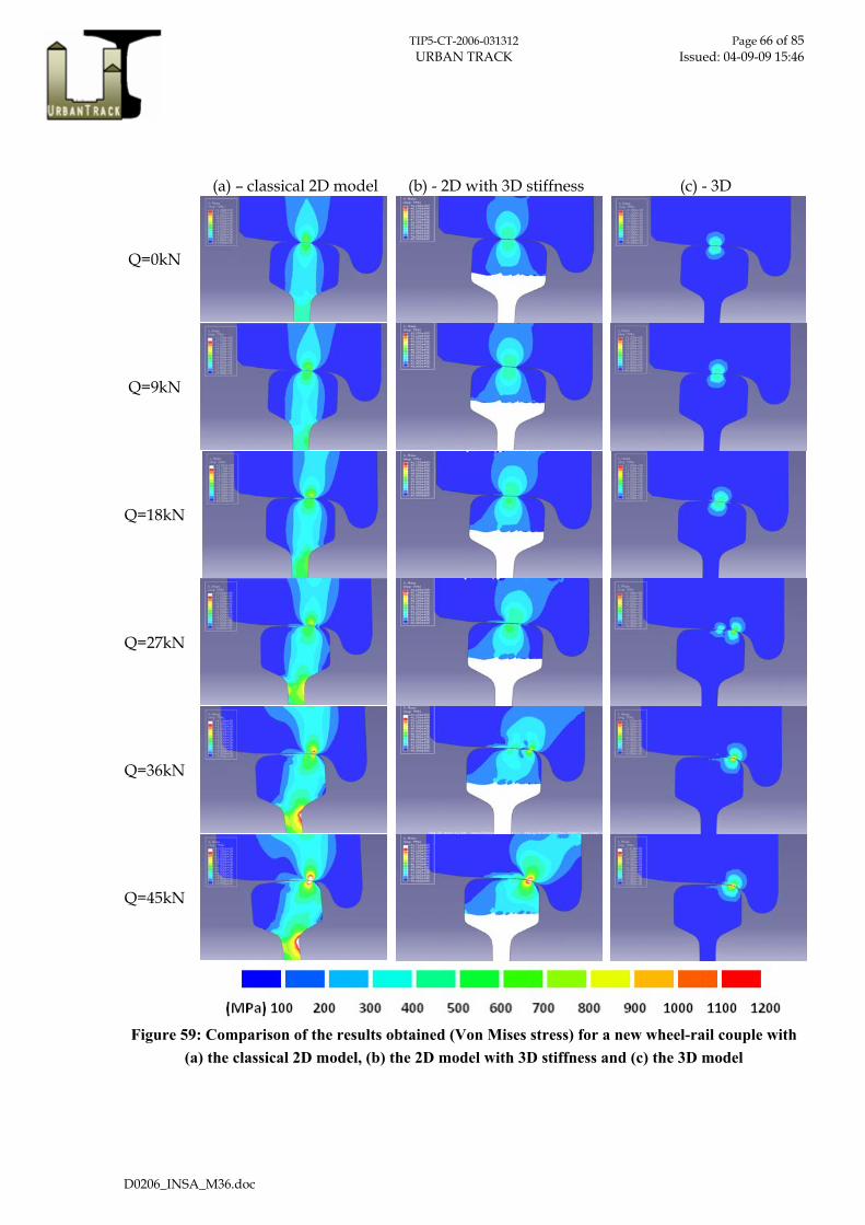
TIP5-CT-2006-031312 Page 66 of 85 URBAN TRACK Issued: 04-09-09 15:46
D0206_INSA_M36.doc
(a) – classical 2D model (b) - 2D with 3D stiffness (c) - 3D
Q=0kN
Q=9kN
Q=18kN
Q=27kN
Q=36kN
Q=45kN
Figure 59: Comparison of the results obtained (Von Mises stress) for a new wheel-rail couple with (a) the classical 2D model, (b) the 2D model with 3D stiffness and (c) the 3D model

TIP5-CT-2006-031312 Page 67 of 85 URBAN TRACK Issued: 04-09-09 15:46
D0206_INSA_M36.doc
4.1.2. An enhanced 2D model of wheel-rail contact at full scale
Contact behaviour strongly depends on the “mechanism effect”: the deformation of the structures of the wheelset and the rails, the stiffness of the foundation of the track, affect the geometry of the contact and therefore its response. The previous 2D model which has been developed presents the advantage to model a complex contact problem at the scale of a hundred µm, while taking into account the main components of the mechanism (i.e. the wheelset, the rails and track stiffness), for a reduced calculation time (i.e. about 1 day on a recent computer using 3 CPU at 3 GHz and 6 Go memory). However, some issues were identified and improvement have been done to model more realistically the “mechanism effect”.
The 2D model is used to represent a 3D problem: of course, the stiffness of the structures are not equivalent. A coarse 3D model (not presented) has been developed to estimate the deformation of the structures under vertical loading. In the case of the previous 2D model, deformation of the web of the rails, the web of the wheels and bending of the shaft is over amplified. According to the coarse 3D model results, the web of both the rails and the wheels have been defined as rigid in the improved model (fig. 60). The elastic modulus of the shaft has been increased, with new values E = 3.1012 Pa and ν = 0.3, to fit the analytical deflection of a beam in a 4-points bending test, see following calculation:
Figure 60: Principle of the wheel-rail contact models with adapted stiffness

TIP5-CT-2006-031312 Page 68 of 85 URBAN TRACK Issued: 04-09-09 15:46
D0206_INSA_M36.doc
The results obtained with such a model are presented figure 59-b. Once the vertical load P of 90 kN is applied, the lateral load Q is progressively applied from 0 kN to 45 kN. Initially, the contact occurs at the centre of the rail which is classical. The contact pressure is still about 950 MPa as expected with Hertz theory in this case. While increasing the lateral load Q, the contact zone displaced toward the active flange and the contact pressure increase as expected. Thanks to the improvement of the wheel and rail web stiffness, the displacement of the railhead ( on figure 58-a) and of the wheel ( on figure 58-a) reach a value close to the one obtained with a 3D model (table 9). The same thing occur for the Von Mises stress level which reaches values close to 1.5 GPa when active flange contact occurred for Q = 45 kN.
In order to verify the reliability of this improved 2D model with 3D stiffness, a 3D model has been developed and the results obtained have been compared with those of such a 2D model.
4.1.3. A 3D model of wheel-rail contact at full-scale
Based on the previously described characteristics, the 3D model of wheel-rail contact (fig. 61) is meshed with C3D8R elements (i.e. linear brick with 8 nodes).
Figure 61: global view of the 2D mesh
The size of the elements in the refined zone (near the contact) is respectively for the rail 400 µm x 400 µm (slave surface) and for the wheel 800 µm x 800 µm (master surface), see figure 62.
The number of C3D8R elements is : - about 170 000 elements for each rail, - about 90 000 elements for the wheelset
The entire model contains about 430 000 elements

TIP5-CT-2006-031312 Page 69 of 85 URBAN TRACK Issued: 04-09-09 15:46
D0206_INSA_M36.doc
(a) (b)
Figure 62: 3D mesh of (a) the new rail and (b) the new wheel The results obtained with such a model are presented figure 59-c. Once the vertical load P of 90 kN is applied, the lateral load Q is progressively applied from 0 kN to 45 kN. As previously observed with the 2D model with 3D stiffness, the contact displaced toward the active flange while lateral load increase as it was expected. Nevertheless, in the 3D model, the contact reach the active flange quicker than with the improved 2D model. A bi-contact is observed for Q = 27 kN with the 3D model while it is necessary to apply at least 36 kN to observe a similar behaviour with the improved 2D model. Moreover, the general level of stress in the rail head of the 2D model always remains slightly higher than in 3D, about 10 to 15% higher. These differences could be explained by the remaining “classical” 2D part of the model near the contact zone which flexibility is lower in 2D than in 3D.
As for a consequence, the improved 2D model is not as representative of the 3D behaviour as expected even if the tendencies observed are similar. Finally, the model chosen to highlight contact characteristics and to draw a parallel with contact reality will be the 3D model.
4.2. WHEEL-RAIL CONTACT CHARACTERISTICS AND PARALLEL TO REALITY
4.2.1. Wheel-rail contact characteristics
In order to highlight wheel-rail contact characteristics as a function of lateral load Q, two 3D models have been developed, the first uses new wheel and rail profiles (fig. 63 and fig. 64) and the second uses worn wheel and rail profiles (fig. 65 and fig. 66). Both contact pressure evolution and plastic deformation are computed on the rail surface. New wheel and rail profiles:
The three main wheel-rail contact configurations (fig. 55) are observed for the left rail: - From Q = 0 kN to Q = 18 kN, a mono-contact is observed which is mostly centered
on the rolling table of the rail with a contact pressure close to 1 GPa. No plastic deformation occurs due to such contact conditions.
- For Q ~ 27 kN, a bi-contact is observed. On the rolling table, the contact pressure decreases progressively while Q increases. On the active flange, the contact pressure increases progressively while Q increases quickly to reach values over 1 GPa (about

TIP5-CT-2006-031312 Page 70 of 85 URBAN TRACK Issued: 04-09-09 15:46
D0206_INSA_M36.doc
1.6 GPa for Q = 27 kN). The consequence is a little plastic deformation of the active flange of the rail.
- For Q =36 kN to Q = 45 kN, a mono-contact is observed on the active flange of the rail. The contact pressure reaches value close to 2.5 GPa which implies a not negligible increase of the plastic deformation up to 3%.
Contact characteristics of the right rail are logical (no active flange contact): contact occurs on the rolling table (around its centre), the contact pressure remains close to 1 GPa and no plastic deformation are observed.
Worn wheel and rail profiles:
Contrary to the new profile case, only one contact configuration is observed for both left and right rail: - From Q = 0 kN to Q = 45 kN, a mono-contact is observed, mostly on the beginning of
the active flange with a maximum contact pressure about 1.4 GPa and maximum plastic deformation of 1.5% for the left rail and 1% for right rail. Contact zone slightly displaces to remains in the top of the active flange for both left and right rails. Contact zone is composed of longitudinal strips. These strips corresponds to the direction of extrusion of the rail profile given by RATP but are also observed locally on real rail surfaces when no singular defects are noted.

TIP5-CT-2006-031312 Page 71 of 85 URBAN TRACK Issued: 04-09-09 15:46
D0206_INSA_M36.doc
Left Rail Right Rail
Q=0kN
Q=9kN
Q=18kN
Q=27kN
Q=36kN
Q=45kN
Figure 63: 3D new wheel-rail couple – Contact pressure on both left and right rail
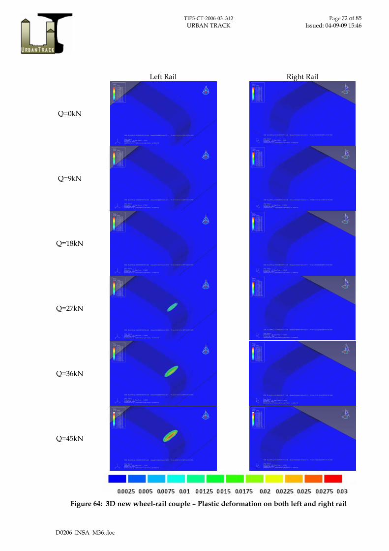
TIP5-CT-2006-031312 Page 72 of 85 URBAN TRACK Issued: 04-09-09 15:46
D0206_INSA_M36.doc
Left Rail Right Rail
Q=0kN
Q=9kN
Q=18kN
Q=27kN
Q=36kN
Q=45kN
Figure 64: 3D new wheel-rail couple – Plastic deformation on both left and right rail

TIP5-CT-2006-031312 Page 73 of 85 URBAN TRACK Issued: 04-09-09 15:46
D0206_INSA_M36.doc
Left Rail Right Rail
Q=0kN
Q=9kN
Q=18kN
Q=27kN
Q=36kN
Q=45kN
Figure 65: 3D worn wheel-rail couple – Contact pressure on both left and right rail

TIP5-CT-2006-031312 Page 74 of 85 URBAN TRACK Issued: 04-09-09 15:46
D0206_INSA_M36.doc
Left Rail Right Rail
Q=0kN
Q=9kN
Q=18kN
Q=27kN
Q=36kN
Q=45kN
Figure 66: 3D worn wheel-rail couple – Plastic deformation on both left and right rail

TIP5-CT-2006-031312 Page 75 of 85 URBAN TRACK Issued: 04-09-09 15:46
D0206_INSA_M36.doc
4.2.2. Parallel to wheel-rail contact reality
A parallel is now drawn between 3D computational results and site reality from which worn profiles have been extracted and previous tribological investigations on the mixture done. Figure 67-a draws a parallel between on-site reality and contact pressure computed with new profile of wheel and rail for Q = 45kN. Figure 67-b draws a similar parallel with worn profiles.
(a)
(b)
Figure 67: On site reality vs. 3D wheel-rail couple with (a) new profile and (b) worn profile
On the left rail of the sharp curve track (line 8), it is interesting to notice that grinding marks remain on the top of the rolling table. Such marks indicate no contact occurs between wheel and rail in this area. With the 3D model, no contact zone also exists on the rolling table for Q = 45 kN (equivalent to severe curving conditions).
Furthermore, an oxidized contact zone is noticed on the external side of the rolling table: wheel-rail contact only occurs partially in this zone contrary to what is observed on the active flange.

TIP5-CT-2006-031312 Page 76 of 85 URBAN TRACK Issued: 04-09-09 15:46
D0206_INSA_M36.doc
For both cases, the contact occurs on the top of the active flange, higher for the new profile than with the old one.
The new profiles shows high level of contact pressure, close to 2.4 GPa. Coupled with the shear stress that exists on active flange contact in curve, this high level of contact pressure could create modifications of the structure of the material such as surface tribological transformation (STT). The STT combined with local contact dynamics (not studied in the present work) may be at the origin of a detachment of particles that mixed with the lubricant to create the mixture of the active flange observed on site.
The worn profiles shows a decrease of about 50 % of both contact pressure (maximum 1.4 GPa) and plastic deformation (maximum 1.5 %) associated with a localisation of the contact area in the lubricated zone of the active flange. Thus remains true whatever the transversal load applied. Such evolution could help minimizing the wear process (lower particles detachment) of the railhead if the mixture formed on the active flange tends to protect the rail instead of damaging it.
To confirm the previous hypothesis, a dynamic model taking into account of both lubricant and wear particles birth is required. Under development at the LaMCoS (INSA), the dynamic coupled Finite Element / Discret Element Model could be helpful in a close future.
4.3. INFLUENCE OF THE FRICTION COEFFICIENT, SIMULATING UNDER AND OVER LUBRICATION, ON THE WHEEL-RAIL CONTACT CHARACTERISTICS
Available at the end of June 2009, the 3D model requires 15 days computation time with 3 Intel Xeon CPU at 3 GHz and 6 Go memory. As for a consequence, the study on the influence of the friction coefficient on the wheel-rail contact characteristics has been performed with the improved 2D model. According to the parallel drawn between the 3D model and the improved 2D model (fig. 59), the presented results have to be considered from a qualitative point of view. The loading studied are equivalent to straight track conditions (Q = 0 kN) and severe curving conditions (Q = 45 kN). Two friction coefficients (µ) have been taken into account to evaluate the extreme lubrication cases: 0.3 (under-lubrication with no lubricant on the active flange) and 0.01 (over-lubrication with lubricant also on rolling table).
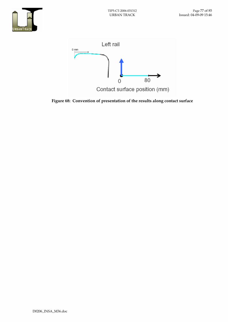
TIP5-CT-2006-031312 Page 77 of 85 URBAN TRACK Issued: 04-09-09 15:46
D0206_INSA_M36.doc
Figure 68: Convention of presentation of the results along contact surface

TIP5-CT-2006-031312 Page 78 of 85 URBAN TRACK Issued: 04-09-09 15:46
D0206_INSA_M36.doc
For each of loading case (Q = 0 kN & Q = 45 kN) and profile (new & worn), contact characteristics are highlighted:
- the localization of the contact patch (fig. 69), - the distribution of the contact pressure (fig. 69), - the equivalent plastic strain (fig. 70).
The results are presented along the contact surface, i.e. function of the arc length on the rail for both left rail and right rail (fig. 68).
(a) (b)
(c) (d)
Figure 69: Contact pressure along contact surface as a function of lateral load and profiles
Straight track conditions (Q = 0 kN), figures 69-a,c and figures 70-a,c
Whatever the friction coefficient used, the contact pressure doesn’t significantly change (less than 1 %). A slight displacement of the contact area is nevertheless noticed for µ = 0.01. This last is 1 mm closer to the active flange with the new profiles. No contact displacement is highlighted with the worn profile case. The plastic deformation remains equal to zero with the new profiles and doesn’t change either in level or repartition with the worn profiles. The friction coefficient evolution doesn’t affect the characteristics of the contact patch. Such a results is logical according to the absence of lateral loading or velocities in such a model.
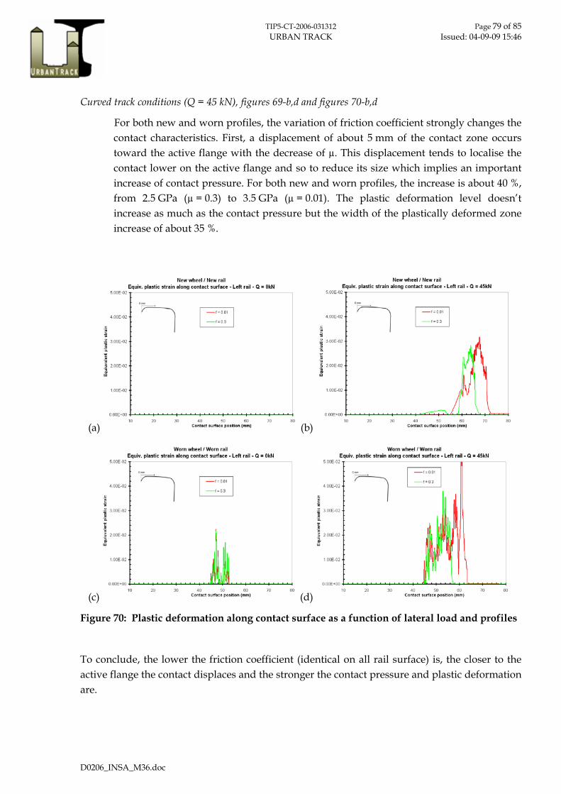
TIP5-CT-2006-031312 Page 79 of 85 URBAN TRACK Issued: 04-09-09 15:46
D0206_INSA_M36.doc
Curved track conditions (Q = 45 kN), figures 69-b,d and figures 70-b,d
For both new and worn profiles, the variation of friction coefficient strongly changes the contact characteristics. First, a displacement of about 5 mm of the contact zone occurs toward the active flange with the decrease of µ. This displacement tends to localise the contact lower on the active flange and so to reduce its size which implies an important increase of contact pressure. For both new and worn profiles, the increase is about 40 %, from 2.5 GPa (µ = 0.3) to 3.5 GPa (µ = 0.01). The plastic deformation level doesn’t increase as much as the contact pressure but the width of the plastically deformed zone increase of about 35 %.
(a) (b)
(c) (d)
Figure 70: Plastic deformation along contact surface as a function of lateral load and profiles
To conclude, the lower the friction coefficient (identical on all rail surface) is, the closer to the active flange the contact displaces and the stronger the contact pressure and plastic deformation are.

TIP5-CT-2006-031312 Page 80 of 85 URBAN TRACK Issued: 04-09-09 15:46
D0206_INSA_M36.doc
5. CONCLUSION
A good lubrication process reduces the wear and the friction in the wheel flange and flange root, meanwhile keeps the rail head dry for optimal adhesion (traction and breaking). Whereas in urban rail networks, wheel rail lubrication in narrow curves is an important topic in terms of maintenance cost, life time and security very few research investigations have been done on this complex problem. As a consequence this work performed by INSA on rail lubrication was exploratory.
The research has been divided in four main parts: First INSA meets lubrication experts for the wheel-rail contact to understand how the
process adjustment and the maintenance are done on RATP networkIII (the tribological approach developed from RATP network study could be transposed to others networks).
Secondly the tribological properties of the mixture are characterised. To do this, sampling is done on RATP network.
Thirdly the test benches used are described, then the formation and the tribological behaviour of the “wear” mixture (initial lubricant + wear particles) investigated.
Fourthly a numerical model will be settled to access to local wheel-rail contact characteristics (i.e. contact geometry evolution during traffic, contact positions on the rail surface, contact pressures, plastic deformation… ) under various lateral loading conditions from straight track to sharp curved track.
Setting on an on-site experimental feedback, RATP has found for one initial lubricant the way to form in situ an efficient mixture. Best practice has defined a “good lubrication” state, and the maintenance policy in term of lubrication is to maintain this state of lubrication. From our own experience, previous work highlighted the same state on others networks (SNCF for example), that’s why this “good lubrication state” was chosen as reference case. It is now obvious that a good lubrication required the formation in situ of a mixture. This mixture is the melting of the initial lubricant and the particles detached from the wheels and rails. Thus the study focused on the tribological study of the mixture.
The chemical composition and the texture of this mixture have been investigated with different specific tools: Photonic Microscope, Environmental Scanning Electronic Microscopy (SEM) and X-ray energy dispersive analysis (EDX).
The mixture rheology has been studied on a Bridgman simulator which allows to reproduce contact pressure and high shearing conditions. Different mixtures sampled on site have been tested and their functioning analysed (range of friction coefficient from 0.005 to 0.015, localisation of the velocity accommodation in the skin (interface) or in the bulk of the mixture).
A roller / plane simulator of INSA was modified in link to the wheel flange-rail active root flange contact configuration. Then tests have been performed in the aim:
III RATP network has been chosen at the beginning of the project for a first investigation, especially to reduce travel
costs.
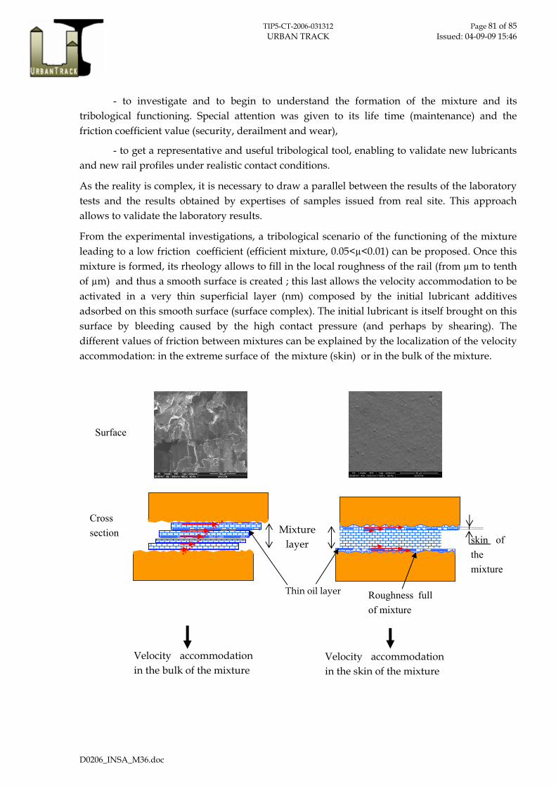
TIP5-CT-2006-031312 Page 81 of 85 URBAN TRACK Issued: 04-09-09 15:46
D0206_INSA_M36.doc
- to investigate and to begin to understand the formation of the mixture and its tribological functioning. Special attention was given to its life time (maintenance) and the friction coefficient value (security, derailment and wear),
- to get a representative and useful tribological tool, enabling to validate new lubricants and new rail profiles under realistic contact conditions.
As the reality is complex, it is necessary to draw a parallel between the results of the laboratory tests and the results obtained by expertises of samples issued from real site. This approach allows to validate the laboratory results.
From the experimental investigations, a tribological scenario of the functioning of the mixture leading to a low friction coefficient (efficient mixture, 0.05<µ<0.01) can be proposed. Once this mixture is formed, its rheology allows to fill in the local roughness of the rail (from µm to tenth of µm) and thus a smooth surface is created ; this last allows the velocity accommodation to be activated in a very thin superficial layer (nm) composed by the initial lubricant additives adsorbed on this smooth surface (surface complex). The initial lubricant is itself brought on this surface by bleeding caused by the high contact pressure (and perhaps by shearing). The different values of friction between mixtures can be explained by the localization of the velocity accommodation: in the extreme surface of the mixture (skin) or in the bulk of the mixture.
Cross section
Surface
skin of the mixture
Mixture layer
Velocity accommodation in the skin of the mixture
Velocity accommodation in the bulk of the mixture
Thin oil layer Roughness full of mixture

TIP5-CT-2006-031312 Page 82 of 85 URBAN TRACK Issued: 04-09-09 15:46
D0206_INSA_M36.doc
The control of the lubrication process requires the control of the initial formation of an efficient mixture and its holding in the contact, which means a specific optimized rheology of the mixture, a localization of the velocity accommodation (surface) with a low friction. Its formation can be in situ or ex situ. Given the state of current knowledge, it does not appear possible to formulate a product (ex situ) whose rheology is similar to that of the mixture and which can be deposited on the active flange of the rail surface. Consequently, it is necessary to orient efforts towards the use of controlled rail-wheel wear to obtain the “right” mixture. Its formation has to be in situ. Thus the two phenomena, leading to the formation of this efficient mixture, have to be investigated:
- the detachment of particles,
- the physico-chemical reactivity of the particles with the initial lubricant (oil + additives) under tribological stresses (pressure, shear).
The mechanisms of the lubrication of the active rail gauge involve complex coupling phenomena, which do not allow elementary parametric studies on site (in practice, the parameters involved are never modified one by one). As for a consequence, a laboratory test developed in this study will allow to finish the understanding and then to investigate new biodegradable (for example) lubricants. Note that the validation of a new lubricant is in progress. This new tribological tool enables to preset new lubricants under realistic contact conditions in laboratory, before to perform qualifying tests on industrial test bench or on site.
The numerical modeling proposed in parallel of the experimental simulations allows investigating the local effects of the local friction and of the contact geometry (i.e. new, worn…) on the local stresses fields and thus on the detachment of particles. Last, but not least, further work should integrate:
- the “right” behavior laws of the materials under stresses as those found under contact, i.e. high hydrostatic pressure and high shear gradients,
- the mixture, which could be taken into account thanks discrete elements modeling
Despite its high prospective level, this study brings experimental and numerical tools:
- to finish the understanding of the lubricating mechanisms involved in the contact in curves, and thus of the tribological functioning of the mixtures,
- to specify more precisely criteria for quantification of the rail lubrication in the aim to control the maintenance,
- to formulate some new lubricants,
- to understand the geometric effects of the wheel and the rail.

TIP5-CT-2006-031312 Page 83 of 85 URBAN TRACK Issued: 04-09-09 15:46
D0206_INSA_M36.doc
Effect of the profiles
Active flange lubrication
RATP lub. cond. µ<0.02 µ<0.1
Effects of the oil additives
Smooth surface
Flows of the mixture
Reality Simulations
Experimental Numerical
Mixture Contact location
Geometry effect
Effect of µ
Location Pressure
“Patine“ (specific surface aspect, i.e. the
good 3rd body to lubricate) 7 trains, Extreme pressure oil
Qualitative validation
AN
AL
YS
ES
60 mm
1 mm
Semi quantitative validation
Sp
ec
if
ic
at
io
n
Life duration of the mixture
CPress (MPa)
750
20 50
Others networks
Profiles
Validation
Specification
Conditions of the mixture formation
Representative test
AdditivesLubricationconditions
Figure 71: Scenario of mechanical-chemical operation of the mixture
TIP5-CT-2006-031312 Page 84 of 85 URBAN TRACK Issued: 04-09-09 15:46
D0206_INSA_M36.doc
References
[ALP96] ALP A., ERDEMIR A. and KUMAR S., Wear, 1996, 191, pp 261-264.
[BEAG75] BEAGLEY T.M, MC EWEN I.J., PRITCHARD C., Wear, 1975, 31, pp 77-88.
[CLAY89] CLAYTON P., DANKS D. and STEELE R.K., Appl. Lubric. Eng , 1989, 45 (8), pp501-506.
[DESC 05] DESCARTES S., DESRAYAUD C., NICCOLINI E., BERTHIER Y., Wear, 2005, 258 (7-8), pp 1081-1090.
[DESC 06] DESCARTES S., BERTHIER Y., Rapport INSA Graissage N°2 V(3). Mesure embarquée de l'état du graissage en courbe. Projet de recherche E04572 SNCF-Insa de Lyon. October 2006.
[DESC 08] DESCARTES S., DESRAYAUD C., BERTHIER Y., Experimental identification and characterisation of the effects of contaminants in the wheel rail contact, Proc. IMech Part F – J. of rail and rapid transit, vol 222, N 2, 2008.
[HOU97] HOU K., KALOUSEK J., MAGEL E., Wear, 1997, 211, pp 134-140.
[ISHI08] ISHIDA M., BAN T., IIDA K., ISHIDA H. and AOKI F., Wear, 2008, 265, pp 1497–1503.
[NICC 02] NICCOLINI E., BERTHIER Y, Progression of the stick/slip zones in a dry wheel-rail contact: updating theories on the basis of tribological reality. 29th Leeds-Lyon Symposium on Tribology. Elsevier Tribology series 41 LEEDS (Royaume-uni Angleterre), 2002-09-03-2002-09-06 p. 845 - 854.
[NICC 05] NICCOLINI E., BERTHIER Y Wheel-rail adhesion : laboratory study of "natural" third body role on locomotives wheels and rails. Wear, 2005, N°258, p. 1172 - 1178.
[SUND08] SUNDH J., OLOFSSON U. and SUNDVALL K., Wear, 2008, 265, pp 1425-1430.
[TELL 04] TELLISKIVI T., OLOFSSON U., Wheel rail wear simulation. Wear, Vol. 257, Issue 11, December 2004, pp 1145-1153
[TOME 02] TOMEOKA M., KABE N., TANIMOTO M., MIYAUCHI E., NAKATA M. (2002). Friction control between wheel and rail by means of onboard lubrication. Wear 253 (2002) pp 124 -29.

TIP5-CT-2006-031312 Page 85 of 85 URBAN TRACK Issued: 04-09-09 15:46
D0206_INSA_M36.doc