d optimald-optimal response surface designs in the presence of random block e)ects

Computational Statistics & Data Analysis 37 (2001) 433–453www.elsevier.com/locate/csda

D-optimal response surface designsin the presence of

random block e)ectsPeter Goos ∗, Martina Vandebroek

Departement Toegepaste Economische Wetenschappen, Katholieke Universiteit Leuven,Wetenschappen, Naamsestraat 69, B-3000 Leuven, Belgium

Received 1 September 2000; received in revised form 1 January 2001; accepted 25 January 2001

Abstract

The purpose of this paper is to help the reader in designing D-optimal blocked experiments. Theblock e)ects are assumed to be random. Therefore, in general, the optimal designs depend on theextent to which observations within one block are correlated. An algorithm is presented that producesD-optimal designs for these cases. However, in three speci5c situations, the optimal design does notdepend on the degree of correlation. These situations include some cases where the block size isgreater than or equal to the number of model parameters, the case of minimum support designs andorthogonally blocked 5rst-order designs. In addition, a relationship is established between the design ofexperiments with random block e)ects and the design of experiments with 5xed block e)ects. Finally,it is shown that orthogonal blocking is an optimal design strategy. c© 2001 Elsevier Science B.V. Allrights reserved.

Keywords: D-optimality; Experimental design; Correlated observations; Orthogonal blocking; Fixedblock e)ects; Random block e)ects

1. Introduction

The theory of optimal designs for regression models usually assumes uncorrelatederrors. However, there are many experimental situations in which this assumptionis invalid because the experimental runs cannot be carried out under homogeneousconditions. For example, the raw material used in a production process may be

∗ Corresponding author.E-mail address: [email protected] (P. Goos).

0167-9473/01/$ - see front matter c© 2001 Elsevier Science B.V. All rights reserved.PII: S 0167-9473(01)00010-X

434 P. Goos, M. Vandebroek / Computational Statistics & Data Analysis 37 (2001) 433–453

obtained in batches in which the quality can vary considerably from one batch toanother. To account for this variation among the batches, a random batch e)ectshould be added to the regression model. In the semi-conductor industry, it is ofinterest to investigate the e)ect of several factors on the resistance in computerchips. Here, measurements are taken using silicon wafers randomly drawn from alarge lot. Therefore, the wafer e)ect should be considered as a random e)ect inthe corresponding model. Chasalow (1992) describes an optometry experiment forexploring the dependence of corneal hydration control on the CO2 level in a gaseousenvironment applied through a goggle covering a human subject’s eyes. Since aresponse is measured for each eye, each human subject’s pair of eyes provide ablock of two possibly correlated observations. Other examples of experiments wherethere might be random block e)ects include agricultural experiments where multiple5elds are used or chemistry experiments where runs are executed on di)erent daysor in di)erent laboratories. The experimental design question in these examples ishow to allocate the levels of the factors under investigation to the blocks. Althoughthere exists an extensive literature on optimal block designs for simple treatmentcomparisons, block designs for regression models have received much less attention.Atkinson and Donev (1989) and Cook and Nachtsheim (1989) propose an exchangealgorithm for the computation of D-optimal regression designs in the presence of5xed block e)ects, whereas Trinca and Gilmour (2000) provide an algorithm toallocate a prespeci5ed set of treatment combinations or design points to a numberof blocks. The latter also assume that the block e)ects are 5xed. The derivationof approximate optimal regression designs in the presence of random block e)ectshas been studied by Atkins (1994), Cheng (1995) and Atkins and Cheng (1999).However, their approximate theory for the design of blocked experiments is of limitedpractical use in industrial environments where the number of blocks is typically small.Cheng (1995) as well as Atkins and Cheng (1995) also describe a special case inwhich the exact optimal design is easy to construct. Chasalow (1992) uses completeenumeration to 5nd exact designs for quadratic regression on one variable whenthere are random block e)ects. However, this approach is computationally intensivewhen more than one factor is under investigation. The analysis of response surfacemodels with random block e)ects is discussed by Khuri (1992), who also derivesgeneral conditions for orthogonal blocking, and by Gilmour and Trinca (2000). Inthis paper, we focus on the construction of exact D-optimal designs for the randomblock e)ects model.

Assume that an experiment consists of n experimental runs arranged in b blocksof sizes k1; : : : ; kb with n =

∑bi=1 ki. When the blocks are random, the model can be

written as

y = XR+ ZS + U; (1)

where y is a vector of n observations on the response of interest, the vector R =[�1; : : : ; �p]′ contains the p unknown 5xed parameters, the vector = [1; : : : ; b]′contains the b random block e)ects and U is a random error vector. The matrices Xand Z are known and have dimension n×p and n× b, respectively. X contains thepolynomial expansions of the levels of the m factors at the n experimental runs. Z

P. Goos, M. Vandebroek / Computational Statistics & Data Analysis 37 (2001) 433–453 435

is of the form

Z = diag[1k1 ; : : : ; 1kb]; (2)

where 1k is a k×1 vector of ones. It is assumed that E(S)=0, E(U)=0, Cov(S)=�2SIb,

Cov(U)=�2UIn, and Cov(S; U)=0. The variance–covariance matrix of the observations

Cov(y) can then be written as

V = �2 In + �2

ZZ′: (3)

If the entries of y are grouped per block,

V = diag[V1; : : : ; Vb]; (4)

where

Vi = �2 (Iki + �1ki1

′ki) (5)

and

� = �2 =�

2 : (6)

As a result, the error structure is compound symmetric. Observations within eachblock are correlated, whereas observations from di)erent blocks are statistically in-dependent. In the sequel of the paper, we will refer to the variance ratio � as thedegree of correlation. If the variance components are known, the best linear unbiasedestimator (BLUE) of the unknown R is given by

R̂= (X′V−1X)−1X′V−1y; (7)

with

Var(R̂) = (X′V−1X)−1: (8)

A design X = [X′1 X′

2 : : : X′b]′, where Xi is that part of X corresponding to the ith

block, is called D-optimal if it maximizes the determinant of the information matrix

M = X′V−1X

=1�2

b∑i=1

X′i

(Iki×ki −

�1 + ki�

1ki1′ki

)Xi

=1�2

{X′X −

b∑i=1

�1 + ki�

(X′i1ki)(X

′i1ki)

′}

: (9)

This expression shows that the optimal design depends on the degree of correlation�. When � → 0, or equivalently �2

→ 0, the design problem degenerates to thecase of complete randomization in which the observations are uncorrelated. When� → ∞, the design problem comes down to designing an experiment with 5xedblocks (see Section 3.1). Finally, note that a model similar to (1) is used in Goosand Vandebroek (2001) to describe split-plot designs. The essential di)erence lies inthe fact that the runs of a split-plot experiment are grouped in whole plots becausethey possess common factor levels for some of the experimental factors. In thispaper, the grouping depends on a certain characteristic of the runs independent of


the factors under investigation. For example, in the optometry experiment, each pairof eyes is considered as a block because they belong to the same person.

In the next section, we consider three special cases in which the D-optimal designdoes not depend on �. In Section 3, we establish a connection between the design ofexperiments in the presence of 5xed block e)ects and the design of experiments inthe presence of random block e)ects and we develop an ePcient blocking algorithmto construct D-optimal designs for model (1). Computational results are presented inSection 4. Finally, it is shown that orthogonal blocking of response surface designsis an optimal design strategy for a given design matrix X.

2. Optimal designs that do not depend on W

In three speci5c situations, the D-optimal design for model (1) does not dependon the variance ratio �. In each case, the optimal block design is based on an optimaldesign for the uncorrelated model

y = XR+ U; (10)

where Cov(U) = �2UIn and y, X and R are de5ned as in the correlated model (1).

2.1. Orthogonally blocked 9rst-order designs

An orthogonal block design that is supported on the points of a D-optimal designfor the uncorrelated model (10) with

X′i1ki = 0; (i = 1; : : : ; b) (11)

is a D-optimal design for model (1). The design so obtained is optimal for anypositive �, such that no prior knowledge of the variance components is needed. Notethat the block size may be heterogeneous.

Condition (11) is a special case of the general conditions for orthogonal blockingof response surface designs derived by Khuri (1992):

X′i1ki =

ki

nX′1n; (i = 1; : : : ; b): (12)

Khuri (1992) shows that, under this condition, the generalized least-squares estimator(7) for all elements of R except the intercept is equivalent to the estimator obtainedby treating the block e)ects as 5xed, but he does not address other design issues.

Assume that the observations are arranged such that (11) holds. The informationmatrix (9) then simpli5es to Morth: =X′X=�2

, which is the information matrix on theunknown parameters in model (10). When the observations are arranged such that(11) does not hold, at least one X′

i1ki �= 0 and the information matrix is of the form(9). The di)erence

Morth: − M =1�2

{b∑

i=1

�1 + ki�

(X′i1ki)(X

′i1ki)

′}


Table 1Optimal block design for the whipped topping experiment

Block 1 Block 2A B C A B C

−1 −1 −1 +1 −1 −1+1 +1 −1 −1 +1 −1+1 −1 +1 −1 −1 +1−1 +1 +1 +1 +1 +1

is then a nonnegative-de5nite matrix. As a result, blocking an experiment such that(11) holds is an optimal design strategy for a given X independent of the designcriterion used. Now, a D-optimal design for the uncorrelated model (10) maximizes|X′X=�2

|. Therefore, arranging the n observations of a D-optimal design for model(10) in blocks such that (11) holds is an optimal design strategy for the random blocke)ects model (1). When the model of interest contains an intercept, (11) changesinto

X′i1ki =

(ki

0

); (i = 1; : : : ; b); (13)

provided that the 5rst column of X corresponds to the intercept. This is shown inAppendix A. However, the conditions can be generalized because the D-optimalitycriterion is invariant to a linear transformation of the factor levels. Therefore, anydesign for which (11) and (13) can be accomplished by applying a linear transfor-mation on the factor levels is D-optimal for the design problem considered here.Consider an experiment to optimize the stability of a whipped topping from Cookand Nachtsheim (1989) to illustrate how the result derived here allows us to con-struct a D-optimal design in the presence of random block e)ects. The amount oftwo emulsi5ers (A and B) and the amount of fat (C) are expected to have an impacton the melting that occurs after the aerosol topping is dispensed. Suppose that theexperimenters are interested in the linear e)ects and the two factor interactions onlyand that two laboratory assistants are available for eight observations. The familiar23 factorial is a D-optimal design with eight observations for estimating the e)ectsof interest in the uncorrelated model. A D-optimal design in the presence of randomblock e)ects is easily obtained by using ABC as the block generator. The resultingdesign is displayed in Table 1. It is easy to verify that condition (11) holds.

Finally, it is clear that conditions (11) and (13) cannot be satis5ed when quadraticterms are included in the model. The same goes for pure linear models and linearmodels with interactions when the block size is an odd number. This is because aD-optimal design for the uncorrelated pure linear model or the linear model withinteractions has factor levels −1 and +1 only.

2.2. Large block size

In some speci5c cases, a D-optimal design for correlated model (1) can be con-structed from the D-optimal approximate design for the uncorrelated model (10)


when the block size is larger than the number of model parameters. Let {x∗1 ; : : : ; x

∗h}

with weights {kw∗1 ; : : : ; kw

∗h} be a D-optimal approximate design for the uncorrelated

model (10). Atkins and Cheng (1999) prove that the D-optimal design for model(1) with b blocks of size k consists of b identical blocks where each design pointxi is replicated kw∗

i times if kw∗i is an integer for each i. The optimal design is then

independent of �. This theorem is only valid when the model contains an intercept.It also requires that the block size k is greater than or equal to the number of pa-rameters p. As a matter of fact, each block is supported on at least h distinct designpoints, such that k ¿ h. In addition, the number of distinct design points h must begreater than or equal to the number of parameters p in order to have a nonsingulardesign.

Well-known situations where all kw∗i can be integer occur in mixture experiments

and in the case of regression on a single explanatory variable. In mixture experiments,the optimal approximate designs for 5rst- and second-order models have equal weighton the s points of a simplex lattice design. D-optimal block designs when k is amultiple of s consist of identical blocks in which the lattice design is replicatedk=s times. The attentive reader will point out that mixture models typically do notcontain an intercept and that the theorem of Atkins and Cheng does not apply in thatcase. However, a linear transformation of the design matrix of a mixture experimentexists such that it does contain a column of ones. This is because the sum of themixture components always equals one. For quadratic regression on one variable, theD-optimal approximate design has weight 1

3 on the points −1; 0 and 1. Therefore, aD-optimal design for quadratic regression on [−1; 1] in the presence of random blocke)ects can be readily obtained when the block size is a multiple of three. Consider anexperiment carried out to investigate the impact of the initial potassium=carbon (K=C)ratio on the desorption of carbon monoxide (CO) in the context of the gasi5cationof coal. The experiment is described in Atkinson and Donev (1992). Let x and ydenote the K=C ratio and the amount of CO desorbed respectively. Further, supposethat four blocks of observations are available to the researcher and that the modelof interest is given by

y = �0 + �1x + �2x2: (14)

If the block size of the experiment is equal to three, a D-optimal design with fourblocks of three observations consists of four identical blocks in which −1; 0 and 1each appear once. Similarly, a D-optimal design with four blocks of six observationseach consists of four identical blocks in which −1; 0 and 1 each appear twice.

The result of Atkins and Cheng has a serious impact on the design of this type ofexperiments. Firstly, no prior knowledge on � is required since the optimal designpoints only depend on model (10). Secondly, rather than using a computationallyintensive blocking algorithm to generate a design with n=bk observations, a k-pointD-optimal design for the uncorrelated model can be used in each block. In occasionswhere not all kw∗

i are integer, the result is useful when the block size k is large withrespect to the number of parameters. In this case, which rarely occurs in practice,the values kw∗

i can be rounded to the nearest integer without serious loss of designePciency.


2.3. Minimum support designs

In this section, we restrict our attention to minimum support designs. A minimumsupport design for a model with p parameters is supported on exactly p distinctpoints x1; : : : ; xp. This class of designs is useful because experimenters are oftenreluctant to the copious use of di)erent factor levels and design points. Using asmaller number of distinct points than p in the experiment would result in a sin-gular information matrix. Cheng (1995) provides a method to construct D-optimalminimum support designs for model (1) by combining a p-point D-optimal designfor the uncorrelated model (10) and a design with b blocks of size k for p treatmentsthat is D-optimal for estimating treatment contrasts. The most famous examples ofD-optimal block designs for treatment contrasts are balanced incomplete block de-signs (BIBDs). An instructive introduction on BIBDs can be found in Cox (1958)and their properties are described thoroughly in Shah and Sinha (1989).

Suppose {x1; : : : ; xp} is a D-optimal design with p observations for the uncor-related model (10) and that a D-optimal block designs for treatment contrasts isavailable with p treatments and b blocks of size k, then using the p design pointsas treatments in the D-optimal block design yields a design that is D-optimal in theclass of block designs with p points and b blocks of size k. Like in Section 2.2,no prior knowledge on � is required and only a small design for the uncorrelatedmodel has to be computed. The main drawback of this approach is that the blocksize should be homogeneous.

As an illustration, consider a modi5ed version of the constrained mixture ex-periment for estimating the impact of three factors on the electric resistivity of amodi5ed acrylonitrile powder described in Atkinson and Donev (1992). The factorsunder investigation are

x1: copper sulphate (CuSO4),x2: sodium thiosulphate (Na2S2O3),x3: glyoxal (CHO)2.

The following constraints were imposed on the factor levels:

0.26 x1 6 0.8,0.26 x2 6 0.8,0.06 x3 6 0.6.

Assume that the model is given by the second-order Sche)Qe polynomial

y =3∑

i=1

�ixi +2∑

i=1

3∑j=i+1

�ijxixj: (15)

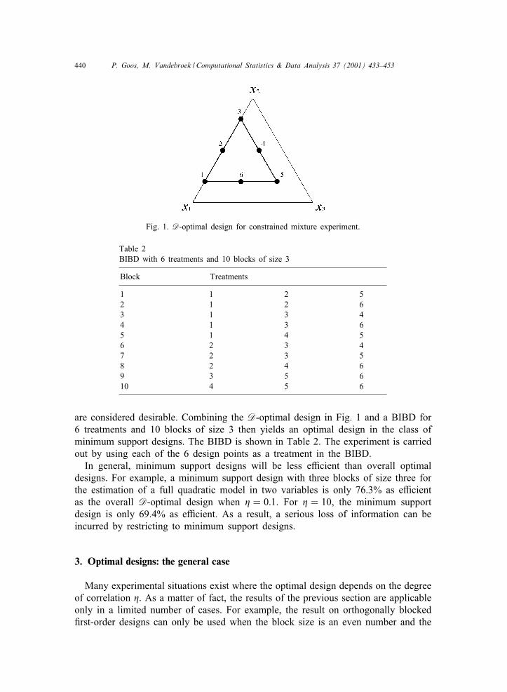
A D-optimal design with six observations for this model is given by the second-order simplex lattice design on the constrained design region. This is illustrated inFig. 1. Now, suppose that 10 experimenters are available and that 30 observations


Fig. 1. D-optimal design for constrained mixture experiment.

Table 2BIBD with 6 treatments and 10 blocks of size 3

Block Treatments

1 1 2 52 1 2 63 1 3 44 1 3 65 1 4 56 2 3 47 2 3 58 2 4 69 3 5 610 4 5 6

are considered desirable. Combining the D-optimal design in Fig. 1 and a BIBD for6 treatments and 10 blocks of size 3 then yields an optimal design in the class ofminimum support designs. The BIBD is shown in Table 2. The experiment is carriedout by using each of the 6 design points as a treatment in the BIBD.

In general, minimum support designs will be less ePcient than overall optimaldesigns. For example, a minimum support design with three blocks of size three forthe estimation of a full quadratic model in two variables is only 76.3% as ePcientas the overall D-optimal design when � = 0:1. For � = 10, the minimum supportdesign is only 69.4% as ePcient. As a result, a serious loss of information can beincurred by restricting to minimum support designs.

3. Optimal designs: the general case

Many experimental situations exist where the optimal design depends on the degreeof correlation �. As a matter of fact, the results of the previous section are applicableonly in a limited number of cases. For example, the result on orthogonally blocked5rst-order designs can only be used when the block size is an even number and the


theorem on minimum support designs in Section 2.3 cannot be used when the numberof support points is allowed to be larger than the number of unknown parameters.

In this section, we show that the design problem at hand is related to that con-sidered in Atkinson and Donev (1989) and Cook and Nachtsheim (1989). We alsopresent a point exchange algorithm to compute exact response surface designs inthe presence of random block e)ects. In Section 4, some computational results arediscussed.

3.1. Fixed block e=ects

If 5xed block e)ects are assumed instead of random block e)ects, the model canbe rewritten as

y = X̃R̃+ ZS + U= W�+ U; (16)

where X̃ and R̃ are the parts of X and R not corresponding to the intercept, W =[X̃ Z]; � = [R̃′ S′]′ and E(U) = 0 and Cov( ) = �2

I. Algorithms to constructD-optimal blocking designs for this model have been proposed by Atkinson andDonev (1989) and by Cook and Nachtsheim (1989). Under model (16), the D-optimaldesign for estimating � is equivalent to the D�̃-optimal design, i.e. the D-optimal

design for model (16) when interest is in estimating R̃ only. In other words, maxi-mizing |W′W| and |X̃′{I −Z(Z′Z)−1Z′}X̃| turns out to be equivalent. In AppendixB, it is shown that

X̃′{I − Z(Z′Z)−1Z′}X̃ = X̃

′X̃ −

b∑i=1

1ki

(X̃′i1ki)(X̃

′i1ki)

′: (17)

The matrix in (17) can be obtained from (A4) when � → ∞. For this reason,the D-optimal designs for model (16) with 5xed blocks and model (1) with randomblocks will be equivalent for large �. Another consequence is that the designs derivedin Section 2 are D-optimal as well when the block e)ects are 5xed instead of random.

Blocked experiments that are generated for 5xed block e)ects models can be usedwhen the blocks are random as well. We have shown that this makes sense if � islarge. However, it is expected that these designs will not be optimal for practicalvalues of �. The algorithms based on the assumption of 5xed block e)ects also failto produce designs when p + b¿n. This is because b block e)ects need to beestimated when the blocks are 5xed rather than random. For these reasons, we havedeveloped an algorithm to compute D-optimal designs in the presence of randomblock e)ects. Designs can be produced as soon as n¿ p.

3.2. Generic point exchange algorithm

Unlike Chasalow (1992), we have chosen to use a point exchange algorithm tocompute D-optimal designs under random block e)ects. This is because enumeratingall possible blocks and designs is a hopeless task when two or more factors are under


investigation and when more than three factor levels are considered. Point exchangealgorithms have been used for a variety of design problems, one of them being theblocking of response surface designs when the block e)ects are 5xed. This topicis treated in Atkinson and Donev (1989) and Cook and Nachtsheim (1989). Thealgorithm of Atkinson and Donev (1989) 5rst computes an n-point starting designwhich is then improved by substituting a design point with a point from the list ofcandidates until no further improvement in D-ePciency can be made. The startingdesign is partly generated in a random fashion and completed by a greedy heuristic.In order to avoid being stuck in a locally optimal design, more than one startingdesign is generated and the exchange procedure is repeated. Each repetition of thesesteps is called a try. In contrast, Cook and Nachtsheim (1989) only use one try. Inorder to obtain a starting design, they compute a p-point design for model (10) anduse these points to compose a nonsingular blocking design. The resulting design isfurther improved by interchanging observations from di)erent blocks.

In the generic algorithm described here, more than one try is used and the start-ing designs are partly composed in a random fashion and completed by sequentiallyadding the candidate point with the largest prediction variance. In order to improvethe initial design, both exchanging design points with candidate points and inter-changing observations from di)erent blocks are considered. The input to the algo-rithm consists of the number of observations n, the number of blocks b, the blocksizes ki (i=1; : : : ; b), the number of model parameters p, the order of the model, thenumber of explanatory variables m and the structure of their polynomial expansion.In addition, an estimate of � must be provided. A reasonable guess is usually satis-factory because the optimal block designs turn out to be optimal for a wide range of�-values. Typically, information on � is available from prior experiments of a sim-ilar kind. Khuri (1992) analyzes an experiment in which the e)ect of temperatureand time on shear strength is investigated and obtains �̂ = 0:2928. The blocks werethe batches of experimental material randomly selected from the warehouse supply.Gilmour and Trinca (2000) analyze an experiment for investigating a mixing processfor pastry dough and obtain �̂ = 10 for one response and �̂ = 1:4 for another. In thepastry dough experiment, all observations within a block were carried out on thesame day. By default, the algorithm assumes a hypercubic design region [ − 1; 1]m

and computes the grid of candidate points as in Atkinson and Donev (1989): thegrid points are chosen from the 2m; 3m; : : : factorial design depending on whether themodel contains linear, quadratic or higher order terms. Alternatively, the user canspecify another set of candidate points. This is important when the design region isrestricted or when it is hyperspherical. In order to 5nd ePcient designs, the set ofcandidates should certainly include cornerpoints and cover the entire design region.For example, the points of a 3m factorial design are not suPcient to 5nd an ePcientdesign for the estimation of a quadratic model on a hyperspherical design region.In that case, star points should be included in the set of candidate points. Furtherdetails on the algorithm are given in Appendix C. It was implemented in Fortran 77and is available from the authors.


4. Computational results

We have generated D-optimal block designs for various combinations of the num-ber of observations n, the number of blocks b and the number of experimentalvariables m. As is mostly done in practice, we have used a 5nite grid of candidatepoints. The resulting designs provide us with interesting insights and show the im-portance of taking into account the randomness of the block e)ects. We also showthat designs generated from a 5nite grid are generally not optimal among all designsand can be improved by using an adjustment algorithm. In the sequel of the paper,we will use the term random block design to refer to a design generated for therandom block e)ects model and the term 5xed block design to refer to a designgenerated for the 5xed block e)ects model.

It turns out that taking into account the compound symmetric error structure of theblocked experiment is especially useful when the number of experimental variablesexceeds two and when the model is not purely linear. When n¿p+b, we were ableto compare the random block designs generated by the algorithm from the previoussection to the 5xed block designs generated by the algorithms of Atkinson and Donev(1989) and Cook and Nachtsheim (1989). Design points were chosen from the 3m

factorial design.Consider the 9-point D-optimal design with three blocks of size three. The op-

timal designs for � 6 3:8790 and � ¿ 3:8790 are displayed in Fig. 2a and b,respectively. These designs are denoted by RBD and FBD, respectively. The designfor � ¿ 3:8790 is denoted by FBD because it coincides with the D-optimal 5xedblock design. An interesting feature of the design for small � is that its projection,obtained by ignoring the blocks, results in the 32 factorial, which is the D-optimaldesign for the uncorrelated model (10). For the design in Fig. 2b, this is not thecase.

In order to compare the D-criterion values of random block designs and 5xedblock designs under di)erent degrees of correlation, we have computed the relative

Fig. 2. D-optimal three-level designs with 3 blocks of size 3 for the full quadratic model in 2 variables.


Fig. 3. Comparison of the D-ePciency of the designs in Fig. 2 for the full quadratic model in 2variables.

D-ePciencies( |X′V−1X||A′V−1A|

)1=p

; (18)

where X is the design matrix of the random block design under consideration andA is the design matrix of the 5xed block design for the same design problem. InFig. 3, the relative ePciency of the random block design in Fig. 2a with respect tothe 5xed block design in Fig. 2b is displayed. RBD outperforms FBD for any smallvalue of �. For � close to zero, the former is more than 3% more ePcient than thelatter. However, the ePciency gain obtained by taking into account the correlationin the design phase decreases as the degree of correlation increases. For �¿ 3:8790,FBD is better than RBD. This is consistent with the fact that the D-optimal designfor random blocks with large � is equal to the D-optimal design for 5xed blocks.


Fig. 4. Comparison of the D-ePciency of the random block designs RBD1 and RBD2 to the 5xedblock design FBD with 6 blocks of 4 observations for the full quadratic model in 4 variables.

The picture for more complicated models looks somewhat di)erent. Consider forexample a full quadratic model in four variables and suppose six blocks of fourobservations are available for experimentation. For this design problem, we havefound one random block design that is optimal for � 6 0:00108 and one that isoptimal for 0:00108 6 �6 2685048:042. Let these designs be denoted by RBD1 andRBD2 respectively. The projection of RBD1 obtained by ignoring the blocks yieldsthe D-optimal design for the uncorrelated full quadratic model in four variables,while the projection of RBD2 is slightly less ePcient. The projection of the 5xedblock design for this design problem (FBD) is not even close to D-optimal for theuncorrelated model. Both RBD1 and RBD2 are compared to the 5xed block designFBD for the same design problem in Fig. 4. For � 6 0:12269, RBD1 is betterthan FBD. However, FBD is outperformed by RBD2 for any practical value of �.Compared to FBD, the D-ePciency is increased by more than 1% for small degreesof correlation and by more than 3% when the degree of correlation exceeds unity.


We obtained similar results for both 5rst and second-order models for other com-binations of n; b and k. In general, we can conclude that D-optimal designs in thepresence of random block e)ects fundamentally di)er from D-optimal designs in thepresence of 5xed block e)ects. While the projection of the random block designs isin many cases D-optimal for the uncorrelated model, this is not at all true for theprojection of the 5xed block design. Therefore, the construction of the random blockdesigns can be seen as assigning observations of a highly ePcient design for theuncorrelated model to blocks in order to obtain an ePcient design for the correlatedmodel. On the contrary, an ePcient design in the presence of 5xed block e)ects isobtained from an inePcient design for the uncorrelated model. Computational resultsalso indicate that the random block designs are robust to misspeci5cation of �. Typ-ically, only one, two or three di)erent random block designs were found for a givendesign problem. As a result, these designs are optimal for wide ranges of �. Preciseprior knowledge of the degree of correlation � is therefore not needed to generateD-optimal random block designs. It should be pointed out that sometimes, unlike theexample given in Fig. 2, the 5xed block design turns out to be the optimal randomblock design as well for models with one and two experimental variables even forrelatively small �. For models with more than two variables, this is no longer thecase since the 5xed block design and the optimal random block design only coincidewhen observations within the same block are nearly perfectly correlated, that is forvery large �.

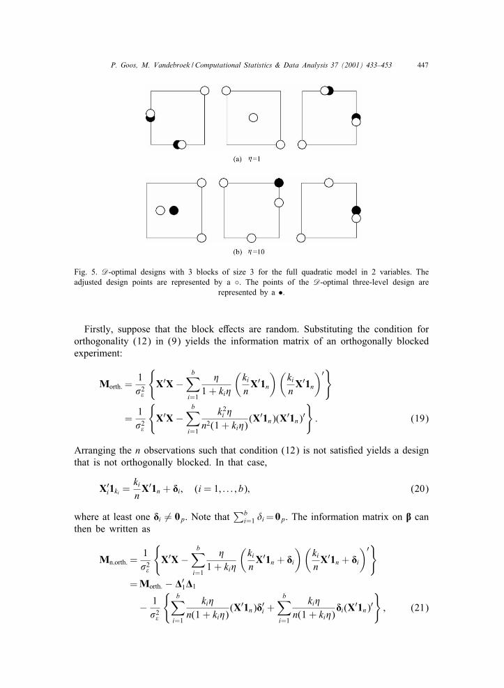
In many cases, designs obtained from a search over a 5nite grid of candidatepoints are not optimal among all designs and can be improved by adjusting theirdesign points. For that purpose, we have applied the adjustment algorithm describedby Donev and Atkinson (1988) to the designs produced by the algorithm of Section3.2. Although the bene5ts of using the adjustment algorithm strongly depend onthe design problem under consideration, it turns out that the smaller the number ofobservations available and the smaller the block sizes, the larger will be the potentialincrease in D-ePciency. The potential increases in design ePciency also tend to belarger for higher degrees of correlation. In Fig. 5, we have displayed the adjusteddesigns with three blocks of size three for quadratic regression on two variables bymeans of a white circle. In order to visualise the di)erence between these designsand the three level designs from Fig. 2, we have displayed the latter by means of ablack bullet. The adjusted design for �=1 is 1.07% more ePcient than its three-levelcounterpart. For � = 10, the adjusted design is 2.12% better.

5. Optimality of orthogonally blocked experiments

The standard textbooks on response surfaces (Box and Draper, 1987; Khuri andCornell, 1987; Myers and Montgomery, 1995), in general, emphasize the importanceof orthogonal blocking since it is desirable that R is estimated independently of theblock e)ects S. The general condition (12) for orthogonal blocking was derived byKhuri (1992). In this section, we show that it is optimal to assign the rows of agiven design matrix X to the blocks such that the resulting design is orthogonallyblocked.


Fig. 5. D-optimal designs with 3 blocks of size 3 for the full quadratic model in 2 variables. Theadjusted design points are represented by a ◦. The points of the D-optimal three-level design are

represented by a •.

Firstly, suppose that the block e)ects are random. Substituting the condition fororthogonality (12) in (9) yields the information matrix of an orthogonally blockedexperiment:

Morth: =1�2

{X′X −

b∑i=1

�1 + ki�

(ki

nX′1n

)(ki

nX′1n

)′}

=1�2

{X′X −

b∑i=1

k2i �

n2(1 + ki�)(X′1n)(X′1n)′

}: (19)

Arranging the n observations such that condition (12) is not satis5ed yields a designthat is not orthogonally blocked. In that case,

X′i1ki =

ki

nX′1n + Ti ; (i = 1; : : : ; b); (20)

where at least one Ti �= 0p. Note that∑b

i=1 �i =0p. The information matrix on R canthen be written as

Mn:orth: =1�2

{X′X −

b∑i=1

�1 + ki�

(ki

nX′1n + Ti

)(ki

nX′1n + Ti

)′}

= Morth: − '′1'1

− 1�2

{b∑

i=1

ki�n(1 + ki�)

(X′1n)T′i +b∑

i=1

ki�n(1 + ki�)

Ti(X′1n)′}

; (21)


where

'1 =√

��

[T1√

1 + k1�T2√

1 + k2�: : :

Tb√1 + kb�

]′:

When the block size is homogeneous and equal to k, (21) becomes

Mn:orth: = Morth: − '′1'1

− 1�2

{b∑

i=1

k�n(1 + k�)

(X′1n)T′i +b∑

i=1

k�n(1 + k�)

Ti(X′1n)′}

= Morth: − '′1'1

− k�n(1 + k�)�2

{(X′1n)

(b∑

i=1

T′i

)+

(b∑

i=1

Ti

)(X′1n)′

}

= Morth: − '′1'1: (22)

As a result, the di)erence

Morth: − Mn:orth: = '′1'1 (23)

is nonnegative de5nite. Therefore, when the block size is homogeneous, orthogonallyblocked designs will be better than designs that are not blocked orthogonally withrespect to any generalized optimality criterion, e.g. the D- and A-optimality criteria,for any given X. Whether orthogonality is a guarantee for optimality when the blocksize is heterogeneous remains an open question.

When the block e)ects are assumed to be 5xed instead of random, it can beshown that orthogonal blocking is an optimal strategy for homogeneous as well asfor heterogeneous block sizes. As is shown in Appendix B, the information matrixon the unknown R̃ parameters as de5ned by the 5xed block e)ects model (16) is

Mf : =1�2

{X̃

′X̃ −

b∑i=1

1ki

(X̃′i1ki)(X̃

′i1ki)

′}

: (24)

If we arrange the n observations such that condition (12) is satis5ed, the design isorthogonally blocked and the information matrix on R̃ becomes

Mf :orth: =1�2

{X̃

′X̃ −

b∑i=1

1ki

(ki

nX̃

′1n

)(ki

nX̃

′1n

)′}

=1�2

{X̃

′X̃ − (X̃

′1n)(X̃

′1n)′

b∑i=1

ki

n2

}

=1�2

{X̃

′X̃ − n−1(X̃

′1n)(X̃

′1n)′}: (25)

If we arrange the n observations such that condition (12) is not satis5ed, thedesign is not orthogonally blocked and the information matrix on R̃ can be written


as

Mf :n:orth: =1�2

{X̃

′X̃ −

b∑i=1

1ki

(ki

nX̃

′1n + Ti

)(ki

nX̃

′1n + Ti

)′}

=1�2

{X̃

′X̃ − n−1(X̃

′1n)(X̃

′1n)′ − '′

2'2} (26)

where '2 = [T1=√

k1 T2=√

k2 : : : Tb=√

kb]′. Now, the di)erence

Mf :orth: − Mf :n:orth: = �−2 '′

2'2 (27)

is nonnegative de5nite. As a result, orthogonally blocked designs will be better forthe estimation of R̃ than designs that are not blocked orthogonally with respect toany generalized optimality criterion, e.g. the D- and A-optimality criteria, for anygiven X̃. Since the D-optimal design for estimating � is equivalent to the D�̃-optimaldesign, orthogonal blocking is a D-optimal blocking strategy for the estimation of�, that is for the estimation of both R̃ and the block e)ects S.

6. Conclusion

In this paper, we have concentrated on the computation and the features of ex-act optimal response surface designs in the presence of random block e)ects. Al-though approximate designs under random block e)ects have received attention byseveral authors, exact designs have been considered only by Chasalow (1992). Hisapproach of complete enumeration is however computationally prohibitive. There-fore, we have developed a point exchange algorithm to compute optimal randomblock designs. These designs substantially di)er from blocked experiments designedfor models with 5xed block e)ects. In addition, they are shown to be optimal forwide ranges of the degree of correlation. This implies that precise prior knowledgeof the degree of correlation is not required to compute D-optimal designs in thepresence of random block e)ects. In the paper, it is also shown that some speci5corthogonally blocked designs are optimal for any degree of correlation �. Two othercases in which the optimal design does not depend on � are described as well. Fi-nally, it was shown that orthogonal blocking is optimal when the block e)ects areassumed to be 5xed, as well as when the block e)ects are assumed to be randomand the block size is homogeneous.

Acknowledgements

The paper was written while the 5rst author was a research assistant of the Fundfor Scienti5c Research–Flanders (Belgium).

Appendix A. D-optimality of orthogonally blocked +rst order designs

Let R= [�0 R̃′]′ and X = [1n X̃] and rewrite model (1) as

y = �01n + X̃R̃+ ZS + U; (A.1)


where �0 is the intercept and R̃ and X̃ are the parts of R and X not correspondingto the intercept. Condition (13) then simpli5es to

X̃′i1ki = 0; (i = 1; : : : ; b): (A.2)

The information matrix on R is given by

X′V−1X =[

1′nV−11n 1′nV

−1X̃X̃

′V−11n X̃

′V−1X̃

]:

The D-optimal design therefore maximizes

|X′V−1X| = (1′nV−11n)|X̃′

V−1X̃ − X̃′V−11n(1′nV

−11n)−11′nV−1X̃|:

Since c1 = 1′nV−11n = �−2

∑bi=1 ki=(1 + ki�) is constant over all possible designs, the

optimal design only depends on

X̃′V−1X̃ − X̃

′V−11n(1′nV

−11n)−11′nV−1X̃: (A.3)

Letting c2i = 1=(1 + ki�) for i = 1; : : : ; b and substituting

X̃′V−1X̃ = �−2

{X̃

′X̃ −

b∑i=1

�1 + ki�

(X̃′i1ki)(X̃

′i1ki)

′}

;

and

X̃′V−11n =

b∑i=1

X̃′iV

−1i 1ki

= �−2

b∑i=1

(X̃

′i1ki −

�1 + ki�

X̃′i1ki1

′ki1ki

)

= �−2

b∑i=1

(X̃

′i1ki −

ki�1 + ki�

X̃′i1ki

)

= �−2

b∑i=1

X̃′i1ki

1 + ki�

= �−2

b∑i=1

c2iX̃′i1ki ;

in (A.3) yields

X̃′X̃ −

b∑i=1

�1 + ki�

(X̃′i1ki)(X̃

′i1ki)

′ − c−11 �−2

(b∑

i=1

c2iX̃′i1ki

)(b∑

i=1

c2iX̃′i1ki

)′;

(A.4)


apart from the constant �−2 . Since (A.4) reduces to X̃

′X̃ when (11) holds, a reason-

ing analogous to that in Section 2.1 can be used to show that assigning observationsto the blocks such that (11) holds is the optimal blocking strategy for a given X̃. AD-optimal design for the uncorrelated model (10) maximizes

|X′X|= (1′n1n)|X̃′X̃ − X̃

′1n(1′n1n)−11′nX̃|

= n∣∣∣∣X̃′

X̃ − 1n(X̃

′1n)(X̃

′1n)′∣∣∣∣ ;

which simpli5es to n|X̃′X̃| when (A.2) holds. Therefore, an orthogonal design that

is supported on the n =∑b

i=1 ki points of a D-optimal design for the uncorrelatedmodel (10) such that (A.2), or equivalently (13), holds, is a D-optimal design formodel (1).

Appendix B. The information matrix on R̃

Assume that the rows in X̃ and Z are grouped per block and that the correspondingpart of the design matrix is denoted by X̃i. The information matrix on R̃ under model(16) is given by

X̃′{I − Z(Z′Z)−1Z′}X̃ = X̃

′X̃ − X̃

′Z(Z′Z)−1Z′X̃: (B.1)

Since Z′Z = diag(k1; : : : ; kb) and thus (Z′Z)−1 = diag[k−11 ; : : : ; k−1

b ], we havethat

Z(Z′Z)−1Z′ = diag[k−11 (1k11

′k1); : : : ; k−1

b (1kb1′kb)]: (B.2)

Expression (B.1) then becomes

X̃′X̃ −

b∑i=1

1ki

(X̃′i1ki)(X̃

′i1ki)

′:

Appendix C. The design construction algorithm

We denote the set of g candidate points by G, the set of b blocks by B and theset of ki not necessarily distinct design points belonging to the ith block of a givendesign D by Di (i = 1; : : : ; b). The D-criterion value of a given design D will bedenoted by D, and the best design found at a given time by the algorithm by D∗. Itsblocks will be denoted by D∗

i (i = 1; : : : ; b) and the corresponding D-criterion valueby D∗. For simplicity, we denote the information matrix of the experiment by M.The singularity while constructing a starting design is overcome by using M + !Iinstead of M with ! a small positive number. Finally, we denote the number of triesby t and the number of the current try by tc. The algorithm starts by specifying theset of grid points G = {1; : : : ; g} and proceeds as follows:


1. Set D∗ = 0 and tc = 1.2. Set M = !I and Di = ∅ (i = 1; : : : ; b).3. Generate starting design.

(a) Randomly choose r(1 6 r 6 p).(b) Do r times:

i. Randomly choose i ∈ G.ii. Randomly choose j ∈ B.iii. If #Dj ¡kj, then Dj = Dj ∪ {i}, else go to step ii.iv. Update M.

(c) Do n− r times:i. Determine i ∈ G with largest prediction variance.ii. Randomly choose j ∈ B.iii. If #Dj ¡kj, then Dj = Dj ∪ {i}, else go to step ii.iv. Update M.

4. Compute M and D. If D = 0, then go to step 2, else continue.5. Set " = 0.6. Evaluate exchanges.

(a) Set � = 1.(b) ∀i ∈ B; ∀j ∈ Di; ∀k ∈ G; j �= k:

i. Compute the e)ect �kij = D′=D of exchanging j by k in the ith block.

ii. If �kij ¿�, then � = �k

ij and store i, j and k.7. If �¿ 1, then go to step 8, else go to step 9.8. Carry out best exchange.

(a) Di = Di \ {j} ∪ {k}.(b) Update M and D.(c) Set " = 1.

9. Evaluate interchanges.(a) Set � = 1.(b) ∀i; j ∈ B; i¡ j; ∀k ∈ Di; ∀l ∈ Dj; k �= l:

i. Compute the e)ect �jlik = D′=D of moving k from

block i to j and l from block j to i.ii. If �jl

ik ¿�, then � = �jlik and store i, j, k and l.

10.If �¿ 1, then go to step 11, else go to step 12.11.Carry out best interchange.

(a) Di = Di \ {k} ∪ {l}.(b) Dj = Dj \ {l} ∪ {k}.(c) Update M and D.(d) Set " = 1.

12.If " = 1, then go to step 5, else go to step 13.13.If D¿D∗, then D∗ = D, ∀i ∈ B : D∗

i = Di.14.If tc ¡ t, then tc = tc + 1 and go to step 2, else stop.

Like in the BLKL algorithm of Atkinson and Donev (1989), the algorithm allowsfor the possibility to consider only grid points with a large prediction variance forinclusion in the design and design points with a small prediction variance for deletion


from the design. This possibility was omitted in the schematic overview of thealgorithm because it provides no additional insights. In order to further speed up thealgorithm, powerful routines were used to update the starting design and to evaluatethe e)ect of the design changes in steps 5 and 8. The basic formulae for updating thedeterminant and the inverse of a nonsingular matrix A after addition or subtractionof an outer product are given by

|A ± uu′| = |A|(1 ± u′A−1u)

and

(A ± uu′)−1 = A−1 ∓ (A−1u)(A−1u)′

1 ± u′A−1u:

Since each design change considered in the algorithm modi5es the information ma-trix of the experiment by adding and subtracting outer products, the determinant andthe inverse of the information matrix can be updated by repeatedly using these basicformulae.

References

Atkins, J.E., 1994. Constructing optimal designs in the presence of random block e)ects, Ph.D.Dissertation, University of California, Berkeley.

Atkins, J.E., Cheng, C.-S., 1999. Optimal regression designs in the presence of random block e)ects.J. Statist. Plann. Inference 77, 321–335.

Atkinson, A., Donev, A., 1989. The construction of exact D-optimum experimental designs withapplication to blocking response surface designs. Biometrika 76, 515–526.

Atkinson, A., Donev, A., 1992. Optimum Experimental Designs. Clarendon Press, Oxford, UK.Box, G., Draper, N., 1987. Empirical Model-Building and Response Surfaces. Wiley, New York.Chasalow, S., 1992. Exact response surface designs with random block e)ects. Ph.D. Dissertation,

University of California, Berkeley.Cheng, C.-S., 1995. Optimal regression designs under random block-e)ects models. Statistica Sinica 5,

485–497.Cook, D., Nachtsheim, C., 1989. Computer-aided blocking of factorial and response-surface designs.

Technometrics 31, 339–346.Cox, D., 1958. Planning of Experiments. Wiley, New York.Donev, A., Atkinson, A., 1988. An adjustment algorithm for the construction of exact D-optimum

experimental designs. Technometrics 30, 429–433.Gilmour, S.G., Trinca, L.A., 2000. Some practical advice on polynomial regression analysis from

blocked response surface designs. Commun. Statist. Theory Methods 29, 2157–2180.Goos, P., Vandebroek, M., 2001. Optimal split-plot designs. J. Quality Technol., to appear.Khuri, A., 1992. Response surface models with random block e)ects. Technometrics 34, 26–37.Khuri, A., Cornell, J., 1987. Response Surfaces: Designs and Analyses. Marcel Dekker, New York.Myers, R., Montgomery, D., 1995. Response Surface Methodology: Process and Product Optimization

using Designed Experiments. Wiley, New York.Shah, K., Sinha, B., 1989. Theory of Optimal Designs. Springer, New York.Trinca, L., Gilmour, S., 2000. An algorithm for arranging response surface designs in small blocks.

Computat. Statist. and Data Anal. 33, 25–43.

d optimald-optimal response surface designs in the presence of random block e)ects

Documents