d a oa - earth observing system p eople in the d a o the list b elo w includes visitors, part time,...
TRANSCRIPT

DAO ATBD Version 1.01
Richard B. Rood, Head Phone (301) 286-8203Data Assimilation O�ce FAX (301) 286-1754Goddard Space Flight Center [email protected], Maryland 20771 http://dao.gsfc.nasa.gov
Algorithm Theoretical Basis Document
for Goddard Earth Observing System
Data Assimilation System (GEOS DAS)
With a Focus on Version 2
Sta��
Data Assimilation O�ce, Goddard Laboratory for Atmospheres
Goddard Space Flight Center, Greenbelt, Maryland
� Refer to this document as:
DAO, 1996: Algorithm Theoretical Basis Document Version 1.01, Data Assimilation O�ce,
NASA's Goddard Space Flight Center.
This ATBD has not been published and should
be regarded as an Internal Report from DAO.
Permission to quote from it should be
obtained from the DAO.
Goddard Space Flight Center
Greenbelt, Maryland 20771November 1996

Preface
The development of the Goddard Earth Observing System (GEOS) Data Assimilation Sys-
tem (DAS) has been a learning process for us all. When the e�ort was started the scope was
not well understood by any of the principal people involved. It was deemed as something
important for the Earth Observing System (EOS), and the expectations were very high.
The Data Assimilation O�ce (DAO) was formed in February 1992 at Goddard Space
Flight Center to develop a data assimilation capability for EOS and the broader NASA
mission. In the following four or so years the progress has been tremendous and hard fought.
The e�ort extends far beyond scienti�c and involves many logistical aspects of developing
a routine production capability. In many ways, we are just getting to the starting line.
The GEOS DAS is a computing e�ort as large, or larger, than any in the world. An
e�ort that is coming on line when the traditional supercomputing paradigm is, by many
counts, collapsing. The computing is characterized by high levels of processor communica-
tions which eliminates any easy solution to the problem. Therefore a tremendous scienti�c
challenge has been compounded by an immense computational challenge. A challenge to
be achieved with about half the historical budget available to comparable e�orts.
This document describes the algorithms proposed by the DAO to be at the basis of the
1998 system provided to coincide with the launch of the AM-1 Platform. It is intended to be
an integrated document. However, the chapters are also designed to stand alone if necessary.
References and acronyms for each chapter are compiled individually. Detailed contents are
given at the beginning of each chapter. Occasionally there is a comment intended to address
the di�culty of writing an interesting algorithm theoretical basis document. You will have
to read it carefully to �nd them
Greenbelt, Maryland R. Rood
November 1996
i
Outline
Chapter 1
Scope of Algorithm Theoretical Basis Document
What is and is not in this document.
Chapter 2
Background
The role of data assimilation in the MTPE enterprise. The DAO Advisory Panels and their
advice. How does the GEOS DAS relate to e�orts at NWP centers. How are requirements
de�ned and linked to MTPE priorities. How to confront the computer problem. What are
the limitations of data assimilation.
Chapter 3
Supporting Documentation
A list of DAO publications that provide more details on the algorithm and algorithm per-
formance.
Chapter 4
GEOS-1 Data Assimilation System
Our �rst data assimilation system. The baseline on which progress is measured.
Chapter 5
The Goddard Earth Observing System - Version 2
Data Assimilation System
It is the system we are validating right now. It is a major development over GEOS-1 and
provides the infrastructure to address the future mission. When you think of reviewing the
algorithm, this is the main course.
ii

Chapter 6
Quality Control of Input Data Sets
This is how we manage the input data sets in the current system.
Chapter 7
New Data Types
How will new data types be incorporated into the GEOS DAS. What are the priorities, and
how are these decisions made. What is the link to MTPE Earth science priorities. This
chapter is at the basis of what needs to be done over the next few years.
Chapter 8
Quality Assessment/Validation of
the GEOS Data Assimilation System
How do we decide when to declare a new version of the assimilation system. It is not easy;
nothing is.
Chapter 9
Evolution from GEOS-2 DAS to GEOS-3 DAS
What will be added to GEOS-2 for the 1998 mission. Improvements to all aspects of the
data assimilation system.
Chapter 10
Summarizing Remarks
Wrapping it up, and what are the risks.
iii

The People in the DAO
The list below includes visitors, part time, and administrative sta�.
NAME TELEPHONE E-MAIL ADDRESS
Almeida, Manina (GSC) (301) 805-7950 [email protected], Pinhas (Tel Aviv U) (301) 805-8334 [email protected], Joe (GSC) (301) 286-3109 [email protected], R. (Bob) (GSFC) (301) 286-3604 [email protected], Steve (GSC) (301) 286-7349 [email protected], Genia (GSC) (301) 286-5182 [email protected], Dennis (GSC) (301) 286-2705 [email protected], L. P. (GSC) (301) 805-6998 [email protected], Yehui (GSC) (301) 286-2511 [email protected], Minghang (ARC) (301) 805-6997 [email protected], Steve (GSFC) (301) 805-7951 [email protected], Austin (GSC) (301) 286-3745 [email protected], Dick (GSC) (301) 805-7963 [email protected], Timothy (NRC) (301) 286-8128 [email protected], Ken (GSC) (301) 805-8336 [email protected], George (HITC) (301) 286-3790 [email protected], Michael (JCESS) (301) 805-7953 [email protected], Greg (USRA) (301) 805-8754 [email protected], Ravi (GSC) (301) 805-7962 [email protected], Jing (GSC) (301) 805-8333 [email protected], Monique (GSC) (301) 805-8440 [email protected], Mark (GSFC) (301) 286-7509 [email protected], Arthur (GSFC) (301) 286-3594 [email protected], Joanna (GSFC) (301) 805-8442 [email protected], Juan Carlos (GSC) (301) 286-4086 [email protected], Mahendra (GSC) (301) 805-6105 [email protected], Yelena (GSC) (301) 805-7952 [email protected], Dave (GSC) (301) 805-7954 [email protected], Jay (JCESS) (301) 805-8334 [email protected], Dave (GSC) (301) 805-7955 [email protected], Yong (GSC) (301) 262-0191 [email protected], Shian-Jiann (GSC) (301) 286-9540 [email protected], Guang Ping (GSC) (301) 805-6996 [email protected], Rob (GSC) (301) 286-9084 [email protected], Peter (JCESS) (301) 805-6960 [email protected], Richard (USRA) (301) 805-7958 [email protected], Wei (USRA) (301) 286-4630 [email protected], Andrea (GSC) (301) 286-3908 [email protected]
iv

NAME TELEPHONE E-MAIL ADDRESS
Nebuda, Sharon (GSC) (301) 286-6543 [email protected], Kazem (GSFC) (301) 805-6930 [email protected], Carlos (GSC) (301) 286-8560 [email protected], Chung-Kyu (JCESS) (301) 286-8695 [email protected], Merritt (GSFC) (301) 286-3468 [email protected], Q. (GSC) (301) 286-7562 [email protected], Vipool (GSC) (301) 286-1445 [email protected], Chris (GSC) (301) 805-8335 [email protected], Lars Peter (USRA) (301) 805-0258 [email protected], Ricky, Head, (GSFC) (301) 286-8203 [email protected], Jean (GSC) (301) 286-3591 [email protected], Robert (GSC) (301) 286-7126 [email protected], Leonid (SUNY) (301) 805-7961 [email protected], Laura (GSC) (301) 286-5691 [email protected], Siegfried (GSFC) (301) 286-3441 [email protected], Meta (GSC) (301) 805-7956 [email protected] Silva, Arlindo (GSFC) (301) 805-7959 [email protected], N. (Siva) (GSC) (301) 805-7957 [email protected], Ivanka (USRA) (301) 805-6999 [email protected], Jim (GSC) (301) 805-8441 [email protected], Susan (GSC) (301) 286-1448 [email protected], Larry (GSC) (301) 286-2510 [email protected], Joe (GSC) (301) 286-2509 [email protected], Felicia (IDEA, Inc.) (301) 286-2466 [email protected], Ricardo (USRA) (301) 286-9117 [email protected],Alice (GSC) (301) 805-1079 [email protected], Bob (GSFC) (301) 286-7600 [email protected], Tonya (GSFC) (301) 286-5210 [email protected], Chung-Yu (John) (GSC) (301) 286-1539 [email protected], Man-Li (GSFC) (301) 286-4087 [email protected], Qiulian (301) 286-0143 [email protected], Runhua (GSC) (301) 805-8443 [email protected], Jose (GSC) (301) 262-2034 [email protected]
v

Contents
1 Scope of Algorithm Theoretical Basis Document 1.1
2 Background 2.1
2.1 Data Assimilation for Mission to Planet Earth . . . . . . . . . . . . . . . . 2.2
2.2 Overview of GEOS Data Assimilation System (DAS) . . . . . . . . . . . . . 2.4
2.3 Scope of GEOS Data Assimilation System (DAS) . . . . . . . . . . . . . . . 2.7
2.4 Data Assimilation O�ce Advisory Panels . . . . . . . . . . . . . . . . . . . 2.10
2.4.1 Comments on Objective Analysis Development . . . . . . . . . . . . 2.10
2.4.2 Comments on Model Development . . . . . . . . . . . . . . . . . . . 2.11
2.4.3 Comments on Quality Control . . . . . . . . . . . . . . . . . . . . . 2.11
2.4.4 Comments on New Data Types . . . . . . . . . . . . . . . . . . . . . 2.11
2.5 Relationship of the GEOS Data Assimilation System to Numerical Weather
Prediction Data Assimilation Systems . . . . . . . . . . . . . . . . . . . . . 2.13
2.6 Customers, Requirements, Product Suite . . . . . . . . . . . . . . . . . . . . 2.16
2.6.1 Customers . . . . . . . . . . . . . . . . . . . . . . . . . . . . . . . . . 2.16
2.6.2 Requirements De�nition Process . . . . . . . . . . . . . . . . . . . . 2.16
2.6.3 Product Suite . . . . . . . . . . . . . . . . . . . . . . . . . . . . . . . 2.18
2.7 Computational Issues . . . . . . . . . . . . . . . . . . . . . . . . . . . . . . 2.20
2.8 The Weak Underbelly of Data Assimilation . . . . . . . . . . . . . . . . . . 2.22
2.9 References . . . . . . . . . . . . . . . . . . . . . . . . . . . . . . . . . . . . . 2.23
2.10 Acronyms . . . . . . . . . . . . . . . . . . . . . . . . . . . . . . . . . . . . . 2.24
2.10.1 General acronyms . . . . . . . . . . . . . . . . . . . . . . . . . . . . 2.24
2.10.2 Instruments . . . . . . . . . . . . . . . . . . . . . . . . . . . . . . . . 2.24
2.11 Advisory Panel Members . . . . . . . . . . . . . . . . . . . . . . . . . . . . 2.26
2.11.1 Science Advisory Panel . . . . . . . . . . . . . . . . . . . . . . . . . 2.26
vi
2.11.2 Computer Advisory Panel . . . . . . . . . . . . . . . . . . . . . . . . 2.27
3 Supporting Documentation 3.1
3.1 DAO Refereed Manuscripts . . . . . . . . . . . . . . . . . . . . . . . . . . . 3.2
3.1.1 Published . . . . . . . . . . . . . . . . . . . . . . . . . . . . . . . . . 3.2
3.1.2 Submitted . . . . . . . . . . . . . . . . . . . . . . . . . . . . . . . . . 3.3
3.1.3 Collaborations . . . . . . . . . . . . . . . . . . . . . . . . . . . . . . 3.3
3.2 DAO O�ce Notes . . . . . . . . . . . . . . . . . . . . . . . . . . . . . . . . 3.4
3.3 Technical Memoranda . . . . . . . . . . . . . . . . . . . . . . . . . . . . . . 3.6
3.4 Other DAO Documents . . . . . . . . . . . . . . . . . . . . . . . . . . . . . 3.8
3.4.1 Planning, MOU and Requirements Documents . . . . . . . . . . . . 3.8
3.4.2 Advisory Panel Reports . . . . . . . . . . . . . . . . . . . . . . . . . 3.8
3.4.3 Conference Abstracts . . . . . . . . . . . . . . . . . . . . . . . . . . 3.8
4 GEOS-1 Data Assimilation System 4.1
4.1 GEOS-1 Multi-year Re-analysis Project . . . . . . . . . . . . . . . . . . . . 4.2
4.2 GEOS-1 DAS Algorithms . . . . . . . . . . . . . . . . . . . . . . . . . . . . 4.4
4.2.1 The GEOS-1 Objective Analysis Scheme (Optimal Interpolation) . . 4.4
4.2.2 GEOS-1 General Circulation Model (GCM) . . . . . . . . . . . . . . 4.5
4.2.3 The Incremental Analysis Update . . . . . . . . . . . . . . . . . . . 4.7
4.3 Performance/Validation of GEOS-1 Algorithms . . . . . . . . . . . . . . . . 4.8
4.3.1 GEOS-1 General Circulation Model . . . . . . . . . . . . . . . . . . 4.8
4.3.1.1 Atmospheric Model Intercomparison Project (AMIP) . . . 4.8
4.3.1.2 Model Impact on Assimilated Data Products . . . . . . . . 4.12
4.3.2 GEOS-1 Data Assimilation System . . . . . . . . . . . . . . . . . . . 4.13
4.3.2.1 Regional Moisture Budgets . . . . . . . . . . . . . . . . . . 4.13
4.3.2.2 East Asian Monsoon . . . . . . . . . . . . . . . . . . . . . . 4.15
4.3.2.3 Atmospheric Chemistry and Transport . . . . . . . . . . . 4.15
4.4 Lessons Learned from the GEOS-1 Re-analysis Project . . . . . . . . . . . . 4.18
4.5 References . . . . . . . . . . . . . . . . . . . . . . . . . . . . . . . . . . . . . 4.21
4.6 Acronyms . . . . . . . . . . . . . . . . . . . . . . . . . . . . . . . . . . . . . 4.24
4.6.1 General acronyms . . . . . . . . . . . . . . . . . . . . . . . . . . . . 4.24
4.6.2 Instruments . . . . . . . . . . . . . . . . . . . . . . . . . . . . . . . . 4.24
vii

5 The Goddard Earth
Observing System { Version 2
Data Assimilation System
(GEOS-2 DAS) 5.1
5.1 Overview of the Data Assimilation Algorithm . . . . . . . . . . . . . . . . . 5.2
5.2 The Physical-space Statistical Analysis System (PSAS) . . . . . . . . . . . 5.3
5.2.1 Design objectives . . . . . . . . . . . . . . . . . . . . . . . . . . . . . 5.3
5.2.2 Background: the statistical analysis equations . . . . . . . . . . . . . 5.4
5.2.3 The global PSAS solver . . . . . . . . . . . . . . . . . . . . . . . . . 5.5
5.2.4 Di�erences between PSAS, OI and spectral variational schemes . . . 5.8
5.2.5 Comparison of the global PSAS solver with the localized OI solver . 5.12
5.2.6 The analysis equations in the presence of forecast bias . . . . . . . . 5.17
5.2.7 Speci�cation of error statistics . . . . . . . . . . . . . . . . . . . . . 5.19
5.2.7.1 Statistical modeling methodology . . . . . . . . . . . . . . 5.19
5.2.7.1.1 General covariance model formulation. . . . . . . . 5.19
5.2.7.1.1.1 Single-level univariate isotropic covariances 5.21
5.2.7.1.1.2 Multi-level univariate covariances . . . . . . 5.22
5.2.7.1.2 Tuning methodology. . . . . . . . . . . . . . . . . 5.23
5.2.7.2 Speci�cation of forecast error statistics . . . . . . . . . . . 5.26
5.2.7.2.1 Forecast height errors. . . . . . . . . . . . . . . . . 5.27
5.2.7.2.1.1 Speci�cation of height error variances . . . 5.27
5.2.7.2.2 Forecast wind errors. . . . . . . . . . . . . . . . . 5.29
5.2.7.2.2.1 Height-coupled wind error component . . . 5.29
5.2.7.2.2.2 Height-decoupled wind error component . . 5.31
5.2.7.2.3 Forecast moisture errors. . . . . . . . . . . . . . . 5.31
5.2.7.3 Speci�cation of observation error statistics . . . . . . . . . 5.31
5.2.7.3.1 Rawinsonde errors. . . . . . . . . . . . . . . . . . 5.31
5.2.7.3.2 TOVS height retrieval errors. . . . . . . . . . . . . 5.32
5.3 The GEOS-2 General Circulation Model . . . . . . . . . . . . . . . . . . . . 5.33
5.3.1 Introduction and Model Lineage . . . . . . . . . . . . . . . . . . . . 5.33
5.3.2 Atmospheric Dynamics . . . . . . . . . . . . . . . . . . . . . . . . . 5.34
5.3.2.1 Horizontal and Vertical Discretization . . . . . . . . . . . . 5.36
5.3.2.2 Time Integration Scheme . . . . . . . . . . . . . . . . . . . 5.38
viii

5.3.2.3 Coordinate Rotation . . . . . . . . . . . . . . . . . . . . . . 5.42
5.3.2.4 Smoothing / Filling . . . . . . . . . . . . . . . . . . . . . . 5.44
5.3.3 Atmospheric Physics . . . . . . . . . . . . . . . . . . . . . . . . . . . 5.48
5.3.3.1 Moist Convective Processes . . . . . . . . . . . . . . . . . . 5.48
5.3.3.1.1 Sub-grid and Large-scale Convection . . . . . . . . 5.48
5.3.3.1.2 Cloud Formation . . . . . . . . . . . . . . . . . . . 5.50
5.3.3.2 Radiation . . . . . . . . . . . . . . . . . . . . . . . . . . . . 5.51
5.3.3.2.1 Shortwave Radiation . . . . . . . . . . . . . . . . . 5.52
5.3.3.2.2 Longwave Radiation . . . . . . . . . . . . . . . . . 5.53
5.3.3.2.3 Cloud-Radiation Interaction . . . . . . . . . . . . 5.54
5.3.3.3 Turbulence . . . . . . . . . . . . . . . . . . . . . . . . . . . 5.55
5.3.3.3.1 Atmospheric Boundary Layer . . . . . . . . . . . . 5.58
5.3.3.3.2 Surface Energy Budget . . . . . . . . . . . . . . . 5.58
5.3.3.4 Gravity Wave Drag . . . . . . . . . . . . . . . . . . . . . . 5.59
5.3.4 Boundary Conditions and other Input Data . . . . . . . . . . . . . . 5.60
5.3.4.1 Topography and Topography Variance . . . . . . . . . . . . 5.60
5.3.4.2 Surface Type . . . . . . . . . . . . . . . . . . . . . . . . . . 5.63
5.3.4.3 Sea Surface Temperature . . . . . . . . . . . . . . . . . . . 5.63
5.3.4.4 Surface Roughness . . . . . . . . . . . . . . . . . . . . . . . 5.66
5.3.4.5 Albedo . . . . . . . . . . . . . . . . . . . . . . . . . . . . . 5.66
5.3.4.6 Sea Ice . . . . . . . . . . . . . . . . . . . . . . . . . . . . . 5.66
5.3.4.7 Snow Cover . . . . . . . . . . . . . . . . . . . . . . . . . . . 5.66
5.3.4.8 Upper Level Moisture . . . . . . . . . . . . . . . . . . . . . 5.67
5.3.4.9 Ground Temperature and Moisture . . . . . . . . . . . . . 5.67
5.4 Combining model and analysis: the IAU process . . . . . . . . . . . . . . . 5.68
5.4.1 Filtering properties of IAU . . . . . . . . . . . . . . . . . . . . . . . 5.70
5.4.2 Impact of IAU on GEOS-1 DAS . . . . . . . . . . . . . . . . . . . . 5.72
5.4.3 Model/analysis interface . . . . . . . . . . . . . . . . . . . . . . . . . 5.72
5.5 References . . . . . . . . . . . . . . . . . . . . . . . . . . . . . . . . . . . . . 5.75
5.6 Acronyms . . . . . . . . . . . . . . . . . . . . . . . . . . . . . . . . . . . . . 5.81
5.6.1 General acronyms . . . . . . . . . . . . . . . . . . . . . . . . . . . . 5.81
5.6.2 Instruments . . . . . . . . . . . . . . . . . . . . . . . . . . . . . . . . 5.81
ix

6 Quality Control of Input Data Sets 6.1
6.1 Quality Control in the GEOS Data Assimilation System . . . . . . . . . . . 6.1
6.2 Pre-processing and Quality Control in GEOS-1 Data Assimilation System . 6.4
6.2.1 Pre-processing: Completeness, Synchronization, Sorting . . . . . . . 6.4
6.2.2 Quality Control during Objective Analysis . . . . . . . . . . . . . . . 6.5
6.3 Pre-processing and Quality Control for GEOS-2 Data Assimilation System . 6.7
6.4 References . . . . . . . . . . . . . . . . . . . . . . . . . . . . . . . . . . . . . 6.8
6.5 Acronyms . . . . . . . . . . . . . . . . . . . . . . . . . . . . . . . . . . . . . 6.9
6.5.1 General acronyms . . . . . . . . . . . . . . . . . . . . . . . . . . . . 6.9
6.5.2 Instruments . . . . . . . . . . . . . . . . . . . . . . . . . . . . . . . . 6.9
7 New Data Types 7.1
7.1 The Incorporation of New Data Types into the GEOS DAS . . . . . . . . . 7.2
7.2 Integration of Science Requirements with Sources of New Data . . . . . . . 7.3
7.2.1 Overview . . . . . . . . . . . . . . . . . . . . . . . . . . . . . . . . . 7.3
7.2.2 Hydrological Cycle . . . . . . . . . . . . . . . . . . . . . . . . . . . . 7.3
7.2.3 Land-Surface/Atmosphere Interaction . . . . . . . . . . . . . . . . . 7.4
7.2.4 Ocean-Surface/Atmosphere Interaction . . . . . . . . . . . . . . . . . 7.5
7.2.5 Radiation (Clouds, Aerosols, and Greenhouse Gases) . . . . . . . . . 7.6
7.2.6 Atmospheric Circulation . . . . . . . . . . . . . . . . . . . . . . . . . 7.7
7.2.6.1 Tropospheric circulation and temperature . . . . . . . . . . 7.7
7.2.6.2 Stratospheric circulation and temperature . . . . . . . . . . 7.8
7.2.7 Constituents . . . . . . . . . . . . . . . . . . . . . . . . . . . . . . . 7.8
7.3 Assimilation of New Data Types into the GEOS DAS . . . . . . . . . . . . 7.9
7.3.1 Statistical Analysis . . . . . . . . . . . . . . . . . . . . . . . . . . . . 7.9
7.3.2 Direct radiance assimilation . . . . . . . . . . . . . . . . . . . . . . . 7.11
7.3.3 Traditional retrieval assimilation . . . . . . . . . . . . . . . . . . . . 7.11
7.3.4 Consistent Assimilation of Retrieved Data (CARD) . . . . . . . . . 7.12
7.3.4.1 Physical Space . . . . . . . . . . . . . . . . . . . . . . . . . 7.12
7.3.4.2 Phase Space . . . . . . . . . . . . . . . . . . . . . . . . . . 7.12
7.4 Implementation . . . . . . . . . . . . . . . . . . . . . . . . . . . . . . . . . . 7.13
7.4.1 Data ow and Computational Issues . . . . . . . . . . . . . . . . . . 7.13
x

7.4.2 Instrument Team Interaction . . . . . . . . . . . . . . . . . . . . . . 7.13
7.4.3 Passive Data Types/Observing System Monitoring . . . . . . . . . . 7.14
7.5 Priorities . . . . . . . . . . . . . . . . . . . . . . . . . . . . . . . . . . . . . 7.15
7.5.1 Priorities grouped by science topic . . . . . . . . . . . . . . . . . . . 7.18
7.5.1.1 Temperature . . . . . . . . . . . . . . . . . . . . . . . . . . 7.19
7.5.1.2 Moisture Assimilation . . . . . . . . . . . . . . . . . . . . . 7.20
7.5.1.3 Convective/Precip. Retrieval Assimilation . . . . . . . . . 7.21
7.5.1.4 Land Surface . . . . . . . . . . . . . . . . . . . . . . . . . . 7.22
7.5.1.5 Ocean Surface . . . . . . . . . . . . . . . . . . . . . . . . . 7.22
7.5.1.6 Constituents . . . . . . . . . . . . . . . . . . . . . . . . . . 7.24
7.5.1.7 Wind pro�le . . . . . . . . . . . . . . . . . . . . . . . . . . 7.25
7.5.1.8 Aerosols . . . . . . . . . . . . . . . . . . . . . . . . . . . . . 7.25
7.5.2 Priorities grouped by satellite . . . . . . . . . . . . . . . . . . . . . . 7.25
7.5.3 Priorities grouped by use in GEOS . . . . . . . . . . . . . . . . . . . 7.27
7.6 References . . . . . . . . . . . . . . . . . . . . . . . . . . . . . . . . . . . . . 7.29
7.7 Acronyms . . . . . . . . . . . . . . . . . . . . . . . . . . . . . . . . . . . . . 7.32
7.7.1 General acronyms . . . . . . . . . . . . . . . . . . . . . . . . . . . . 7.32
7.7.2 Instruments . . . . . . . . . . . . . . . . . . . . . . . . . . . . . . . . 7.32
8 Quality Assessment/Validation of the GEOS Data Assimilation System 8.1
8.1 Validation for Earth-science Data Assimilation . . . . . . . . . . . . . . . . 8.1
8.2 Overview of GEOS-2 Quality Assessment/Validation . . . . . . . . . . . . . 8.4
8.2.1 System Validation . . . . . . . . . . . . . . . . . . . . . . . . . . . . 8.4
8.2.2 Scienti�c Evaluation . . . . . . . . . . . . . . . . . . . . . . . . . . . 8.5
8.2.3 Monitoring . . . . . . . . . . . . . . . . . . . . . . . . . . . . . . . . 8.5
8.2.4 Infrastructure . . . . . . . . . . . . . . . . . . . . . . . . . . . . . . . 8.6
8.3 GEOS-2 Validation Process . . . . . . . . . . . . . . . . . . . . . . . . . . . 8.7
8.3.1 The GEOS-1 Baseline . . . . . . . . . . . . . . . . . . . . . . . . . . 8.7
8.3.1.1 Validated Features (Successes) of the GEOS-1 DAS . . . . 8.7
8.3.1.1.1 Low Frequency Variability. . . . . . . . . . . . . . 8.7
8.3.1.1.2 Short Term Variability. . . . . . . . . . . . . . . . 8.8
8.3.1.1.3 Climate Mean. . . . . . . . . . . . . . . . . . . . . 8.8
xi

8.3.1.1.4 Stratosphere . . . . . . . . . . . . . . . . . . . . . 8.9
8.3.1.2 De�ciencies of the GEOS-1 DAS . . . . . . . . . . . . . . . 8.9
8.3.2 Distillation of the GEOS-1 Baseline . . . . . . . . . . . . . . . . . . 8.13
8.3.3 GEOS-2 Validation . . . . . . . . . . . . . . . . . . . . . . . . . . . . 8.14
8.3.3.1 Relative Validation . . . . . . . . . . . . . . . . . . . . . . 8.15
8.3.3.1.1 O-F statistics. . . . . . . . . . . . . . . . . . . . . 8.15
8.3.3.1.2 QC statistics. . . . . . . . . . . . . . . . . . . . . . 8.15
8.3.3.1.3 A-F spectra, time means. . . . . . . . . . . . . . . 8.15
8.3.3.1.4 O-A statistics . . . . . . . . . . . . . . . . . . . . 8.16
8.3.3.1.5 Forecast skill - Anomaly Correlations . . . . . . . 8.16
8.3.4 Absolute Validation . . . . . . . . . . . . . . . . . . . . . . . . . . . 8.16
8.4 New Approaches to Validation . . . . . . . . . . . . . . . . . . . . . . . . . 8.18
8.5 GEOS-2 Validation Tasks . . . . . . . . . . . . . . . . . . . . . . . . . . . . 8.20
8.6 References . . . . . . . . . . . . . . . . . . . . . . . . . . . . . . . . . . . . . 8.21
8.7 Acronyms . . . . . . . . . . . . . . . . . . . . . . . . . . . . . . . . . . . . . 8.26
8.7.1 General acronyms . . . . . . . . . . . . . . . . . . . . . . . . . . . . 8.26
8.7.2 Instruments . . . . . . . . . . . . . . . . . . . . . . . . . . . . . . . . 8.26
9 Evolution from GEOS-2 DAS to GEOS-3 DAS 9.1
9.1 The Path from 1996 to 1998/GEOS-2 to GEOS-3 . . . . . . . . . . . . . . . 9.3
9.2 Primary System Requirements for GEOS-3 . . . . . . . . . . . . . . . . . . 9.4
9.2.1 Output Data . . . . . . . . . . . . . . . . . . . . . . . . . . . . . . . 9.4
9.2.1.1 Fields . . . . . . . . . . . . . . . . . . . . . . . . . . . . . . 9.4
9.2.1.2 Resolution (space) . . . . . . . . . . . . . . . . . . . . . . . 9.4
9.2.1.3 Resolution (time) . . . . . . . . . . . . . . . . . . . . . . . 9.5
9.2.1.4 Format . . . . . . . . . . . . . . . . . . . . . . . . . . . . . 9.5
9.2.1.5 Delivery Time . . . . . . . . . . . . . . . . . . . . . . . . . 9.5
9.2.1.6 Delivery Rate . . . . . . . . . . . . . . . . . . . . . . . . . 9.5
9.2.1.7 Scienti�c Quality . . . . . . . . . . . . . . . . . . . . . . . . 9.5
9.2.2 Input Data . . . . . . . . . . . . . . . . . . . . . . . . . . . . . . . . 9.6
9.2.2.1 Assimilated Data . . . . . . . . . . . . . . . . . . . . . . . 9.6
9.2.2.2 Boundary Conditions . . . . . . . . . . . . . . . . . . . . . 9.6
xii
9.2.3 Objective Analysis Attributes . . . . . . . . . . . . . . . . . . . . . . 9.6
9.2.3.1 Data Pre-processing QC Software . . . . . . . . . . . . . . 9.6
9.2.3.2 ADEOS, ERS-1, and DMSP Pre-processing . . . . . . . . . 9.7
9.2.3.3 Assimilate Non-state Variables (Observation Operator) . . 9.7
9.2.3.4 Non-separable forecast error correlations . . . . . . . . . . 9.7
9.2.3.5 State Dependent Vertical Correlations . . . . . . . . . . . . 9.7
9.2.3.6 Anisotropic Horizontal Forecast Error Correlations . . . . . 9.7
9.2.3.7 On-line Continuous Forecast Error Variance Estimation . . 9.7
9.2.4 Model Attributes . . . . . . . . . . . . . . . . . . . . . . . . . . . . . 9.8
9.2.4.1 Koster/Suarez Land Surface Parameterization . . . . . . . 9.8
9.2.4.2 Hybridized Koster/Suarez/Sellers Land Surface Parameter-
ization . . . . . . . . . . . . . . . . . . . . . . . . . . . . . 9.8
9.2.4.3 Lin{Rood Tracer Advection Scheme . . . . . . . . . . . . . 9.8
9.2.4.4 Improved Gravity Wave Drag Parameterization . . . . . . 9.8
9.2.4.5 RAS-2 Cloud Scheme With Downdrafts . . . . . . . . . . . 9.9
9.2.4.6 Cloud Liquid Water . . . . . . . . . . . . . . . . . . . . . . 9.9
9.2.4.7 Moist Turbulence . . . . . . . . . . . . . . . . . . . . . . . 9.9
9.2.4.8 Variable Cloud Base . . . . . . . . . . . . . . . . . . . . . . 9.9
9.2.4.9 On-line Tracer Advection of O3, N2O, and CO . . . . . . . 9.9
9.2.5 Computing . . . . . . . . . . . . . . . . . . . . . . . . . . . . . . . . 9.9
9.2.5.1 Cost . . . . . . . . . . . . . . . . . . . . . . . . . . . . . . . 9.9
9.2.5.2 Hardware . . . . . . . . . . . . . . . . . . . . . . . . . . . . 9.10
9.2.5.3 Software . . . . . . . . . . . . . . . . . . . . . . . . . . . . 9.10
9.2.5.4 Network . . . . . . . . . . . . . . . . . . . . . . . . . . . . . 9.10
9.2.5.5 Performance . . . . . . . . . . . . . . . . . . . . . . . . . . 9.10
9.2.6 Validation/Monitoring . . . . . . . . . . . . . . . . . . . . . . . . . . 9.10
9.2.6.1 Scienti�c Evaluation . . . . . . . . . . . . . . . . . . . . . . 9.10
9.2.6.2 Validation Testing . . . . . . . . . . . . . . . . . . . . . . . 9.11
9.2.6.3 Monitoring . . . . . . . . . . . . . . . . . . . . . . . . . . . 9.11
9.2.7 Interfaces . . . . . . . . . . . . . . . . . . . . . . . . . . . . . . . . . 9.11
9.2.7.1 With EOSDIS . . . . . . . . . . . . . . . . . . . . . . . . . 9.11
9.2.8 Documentation . . . . . . . . . . . . . . . . . . . . . . . . . . . . . . 9.11
xiii

9.2.8.1 Algorithm Theoretical Basis Document (ATBD) . . . . . . 9.11
9.2.8.2 Interface Control Document . . . . . . . . . . . . . . . . . 9.11
9.2.8.3 Normal Life-cycle Documents . . . . . . . . . . . . . . . . . 9.11
9.2.9 Schedule . . . . . . . . . . . . . . . . . . . . . . . . . . . . . . . . . . 9.12
9.2.9.1 Operational . . . . . . . . . . . . . . . . . . . . . . . . . . . 9.12
9.2.9.2 Frozen . . . . . . . . . . . . . . . . . . . . . . . . . . . . . 9.12
9.3 Development of Objective Analysis (PSAS) . . . . . . . . . . . . . . . . . . 9.13
9.3.1 Assimilation of observables which are not state variables . . . . . . . 9.13
9.3.2 Account of forecast error bias in the statistical analysis equation . . 9.14
9.3.2.1 A framework for forecast bias estimation. . . . . . . . . . . 9.15
9.3.2.2 Sequential bias estimation. . . . . . . . . . . . . . . . . . . 9.16
9.3.3 Improvement of error correlation models . . . . . . . . . . . . . . . . 9.16
9.3.3.1 Anisotropic correlation models . . . . . . . . . . . . . . . . 9.17
9.4 Development of GEOS GCM . . . . . . . . . . . . . . . . . . . . . . . . . . 9.19
9.4.1 Monotonic, Uptream Tracer Advection . . . . . . . . . . . . . . . . . 9.21
9.4.2 Prognostic Cloud Water . . . . . . . . . . . . . . . . . . . . . . . . . 9.21
9.4.2.1 General description of Development . . . . . . . . . . . . . 9.21
9.4.2.2 Motivation for the development . . . . . . . . . . . . . . . 9.22
9.4.2.3 Interface with new observational data types . . . . . . . . . 9.23
9.4.2.4 Description of the algorithm . . . . . . . . . . . . . . . . . 9.23
9.4.2.5 Strengths and Weaknesses of Prognostic Cloud Water Algo-
rithm . . . . . . . . . . . . . . . . . . . . . . . . . . . . . . 9.24
9.4.3 Land-Surface Model . . . . . . . . . . . . . . . . . . . . . . . . . . . 9.25
9.5 Development of QC . . . . . . . . . . . . . . . . . . . . . . . . . . . . . . . 9.27
9.6 Incorporation of New Input Data Sets . . . . . . . . . . . . . . . . . . . . . 9.34
9.6.1 Improved Treatment Temperature Sounders . . . . . . . . . . . . . . 9.34
9.6.2 Assimilation of surface marine winds . . . . . . . . . . . . . . . . . . 9.35
9.6.3 Assimilation of Satellite Retrievals of Total Precipitable Water and
Surface Precipitation/TRMM . . . . . . . . . . . . . . . . . . . . . . 9.37
9.6.3.1 Assimilation methodology . . . . . . . . . . . . . . . . . . . 9.38
9.6.3.2 Data Source . . . . . . . . . . . . . . . . . . . . . . . . . . 9.38
9.6.4 Constituent Assimilation . . . . . . . . . . . . . . . . . . . . . . . . 9.39
9.7 Advanced Research Topics . . . . . . . . . . . . . . . . . . . . . . . . . . . . 9.41
xiv

9.7.1 Retrospective Data Assimilation . . . . . . . . . . . . . . . . . . . . 9.41
9.7.2 Diabatic Dynamic Initialization . . . . . . . . . . . . . . . . . . . . . 9.45
9.7.3 Vertical Structure of Model . . . . . . . . . . . . . . . . . . . . . . . 9.46
9.7.4 Potential Vorticity Based Model . . . . . . . . . . . . . . . . . . . . 9.46
9.7.5 Regional Applications of the Global Assimilation System . . . . . . 9.46
9.7.6 Advanced Advection Modeling . . . . . . . . . . . . . . . . . . . . . 9.47
9.7.7 Data Assimilation with the IASI Instrument . . . . . . . . . . . . . 9.47
9.7.8 Constituent Data Assimilation . . . . . . . . . . . . . . . . . . . . . 9.47
9.7.9 New Methods to Study Carbon Monoxide Chemistry . . . . . . . . . 9.47
9.8 References . . . . . . . . . . . . . . . . . . . . . . . . . . . . . . . . . . . . . 9.49
9.9 Acronyms . . . . . . . . . . . . . . . . . . . . . . . . . . . . . . . . . . . . . 9.55
9.9.1 General acronyms . . . . . . . . . . . . . . . . . . . . . . . . . . . . 9.55
9.9.2 Instruments . . . . . . . . . . . . . . . . . . . . . . . . . . . . . . . . 9.55
10 Summary of Algorithm Theoretical Basis Document 10.1
10.1 Summary of Algorithm Theoretical Basis Document . . . . . . . . . . . . . 10.1
10.2 Risks . . . . . . . . . . . . . . . . . . . . . . . . . . . . . . . . . . . . . . . . 10.5
xv

List of Figures
2.1 GEOS Data Assimilation System. See text for details. . . . . . . . . . . . . 2.5
2.2 Wavelet analysis of moisture ux over the United States from GEOS-1. . . 2.9
4.1 GEOS-1 GCM outgoing longwave radiation (OLR) time series. . . . . . . . 4.10
4.2 Relative ranks of AMIP GCMs. . . . . . . . . . . . . . . . . . . . . . . . . . 4.11
4.3 GEOS-1 GCM longwave cloud forcing for northern hemisphere. . . . . . . . 4.14
4.4 Time series of GEOS-1 moisture ux. . . . . . . . . . . . . . . . . . . . . . 4.16
4.5 Carbon monoxide (CO) model comparision. . . . . . . . . . . . . . . . . . . 4.19
5.1 PSAS nested pre-conditioned conjugate gradient solver. Routine cg main() contains
the main conjugate gradient driver. This routine is pre-conditioned by cg level2(),
which solves a similar problem for each region. This routine is in turn pre-conditioned
by cg level1() which solves the linear system univariately. See text for details. . 5.7
5.2 Power spectra as a function of spherical harmonic total wavenumber for PSAS
(solid) and OI (points) analysis increments of geopotential height at 500 hPa
(5 case average, see table 5.1). Units: m2. . . . . . . . . . . . . . . . . . . . 5.14
5.3 As in �g. 1, but for 500 hPa relative vorticity. Units: 10�15s�2. . . . . . . . 5.15
5.4 As in �g. 1, but for 500 hPa divergence. Units: 10�15s�2: . . . . . . . . . . 5.15
5.5 Bias (time-mean) and standard deviation of radiosonde observation minus 6-
hour forecast residuals (O-F) for the last 10 days of a one-month assimilation
experiment (February 1992). See text for details. . . . . . . . . . . . . . . . 5.16
5.6 Analysis error as a function of the scalar gain coe�cient K, when bias is not
explicitly accounted for in the analysis, for the scalar example presented in
section 5.2.6. The dotted horizontal line indicates the optimal analysis error
level, obtained when bias is explicitly accounted for in the analysis equation. 5.20
5.7 Compactly supported single-level correlation model and Legendre coe�cients. 5.22
5.8 Compactly supported spline cross-correlation function. . . . . . . . . . . . . 5.23
5.9 Sample and tuned model covariances for 500hPa North-American rawinsonde
height observed-minus-forecast residuals. . . . . . . . . . . . . . . . . . . . 5.26
xvi

5.10 Square-root of zonal average of forecast height error variances estimated from
radiosondes (eq. 5.80, open circles), modi�ed TOVS height innovation vari-
ances (�sTOV Sj
�2���TOVSu
�2, closed circles), and forecast height error vari-
ances estimated from TOVS (eq. 5.82, solid line). Monthly means for De-
cember 1991, at 250 hPa. Units: meters . . . . . . . . . . . . . . . . . . . . 5.28
5.11 Monthly means for December 1991 of radiosonde height innovations at 50 hPa
(open circles), and zonally symmetric �t (solid line). Units: meters . . . . . 5.30
5.12 Stencil showing the position and indexing of the prognostic �elds u, v, �, and
�. . . . . . . . . . . . . . . . . . . . . . . . . . . . . . . . . . . . . . . . . . . 5.37
5.13 Vertical placement and index notation for sigma levels in the GEOS-2 GCM 5.38
5.14 Vertical distribution used in the 70-level GEOS-2 GCM. . . . . . . . . . . . 5.39
5.15 Vertical distribution used in the lowest 10 levels of the GEOS-2 GCM. . . . 5.40
5.16 Rotation parameters used in the GEOS-2 GCM. . . . . . . . . . . . . . . . 5.43
5.17 Wind Speed, Vorticity, and Divergence at 1 hPa using the rotated and non-
rotated 2� x 2:5� 70-level GEOS DAS. . . . . . . . . . . . . . . . . . . . . . 5.45
5.18 Shapiro �lter response function used in the 2� x 2:5�GEOS-2 GCM. . . . . 5.47
5.19 GEOS-2 GCM Critical Relative Humidity for Clouds. . . . . . . . . . . . . 5.51
5.20 Comparison between the Lanczos and mth-order Shapiro �lter response func-
tions for m = 2, 4, and 8. . . . . . . . . . . . . . . . . . . . . . . . . . . . . 5.62
5.21 GEOS-2 GCM Surface Type Compinations at 2� x 2:5� resolution. . . . . . 5.64
5.22 GEOS-2 GCM Surface Type Descriptions. . . . . . . . . . . . . . . . . . . . 5.65
5.23 Schematic of the incremental analysis update (IAU) scheme employed in the GEOS
DAS. Statistical analyses (OI or PSAS) are performed at synoptic times (0000, 0600,
1200 and 1800 UTC). The assimilation is restarted three hours prior to the analysis
time (heavy dashed lines), and the model is integrated forward for 6 hours using the
analysis increments as constant forcing (data in uence shown by shaded regions).
At the end of the IAU interval, an un-forced forecast is made (dotted line) to provide
the �rst guess for the next analysis. . . . . . . . . . . . . . . . . . . . . . . . . 5.68
5.24 Amplitude of the IAU response function as a function of the disturbance
period in hours. Results are shown for 3 values of the growth/decay rate,
� = 0 (neutral case, solid), 1=� = 12 hours (dashed) and 1=� = 6 hours
(dotted). See Bloom et al. 1996 for details. . . . . . . . . . . . . . . . . . . . 5.70
5.25 Surface Pressure Tendency traces at a gridpoint over North America, results dis-
played from every time-step over the course of a 1-day assimilation: IAU (heavy
solid); no IAU (light solid); model forecast, no data assimilation heavy dashed). . . 5.71
5.26 Globally averaged precipitation, plotted in 10 minute intervals, for a 24 hour period.
IAU (solid) and non-IAU (dashed) results. . . . . . . . . . . . . . . . . . . . . . 5.73
xvii

5.27 O-F standard deviations for geopotential heights. Four cases include: IAU, July
1978 (heavy solid); no IAU, July 1978 (heavy dashed); IAU, January 1978 (light
solid); no IAU, January 1978 (light dashed). a) Rawinsondes over North America,
b) TOVS-A retrievals over oceans. . . . . . . . . . . . . . . . . . . . . . . . . 5.74
6.1 Number of NESDIS TOVS retrievals for August 1985 . . . . . . . . . . . . 6.5
9.1 Example of an anisotropic univariate correlation model with a spatially vary-
ing length scale. The left panel shows the prescribed length-scale as a func-
tion of latitude. The shaded contour plots are one-point correlation maps at
various latitudes. The contour interval is 0.1. . . . . . . . . . . . . . . . . . 9.18
9.2 Zonal mean climate radiative diagnostics from GEOS-2 model simulation.
Compared with the GEOS-2 results shown in Chapter 4 and in Molod et
al. (1996) there are �rst order improvements in these quantities. Note in
particular the longwave cloud forcing in middle latitudes which show a sub-
stantial increase compared with the earlier simulations. . . . . . . . . . . . 9.20
9.3 Data ow diagram of the Quality Control aspects of the proposed NCEP
Global Assimilation System (PART I). See text for details. . . . . . . . . . 9.30
9.4 Data ow diagram of the Quality Control aspects of the proposed NCEP
Global Assimilation System (PART II). See text for details. . . . . . . . . . 9.31
9.5 Data ow diagram for the GEOS-3 quality control system. . . . . . . . . . . 9.33
9.6 First tests of NSCAT data with the GEOS assimilation system. . . . . . . . 9.36
9.7 Radiosonde network composed of 33 stations observing winds and heights
every 12 hours (same as Fig. 2 of Cohn and Todling 1996). . . . . . . . . . 9.42
9.8 ERMS analysis error in total energy for (a) the Kalman �lter (upper curve)
and �xed-lag Kalman smoother (lower curves); and (b) the adaptive CEC
�lter and corresponding �xed{lag smoother. . . . . . . . . . . . . . . . . . 9.42
9.9 Analysis error standard deviation in the height �eld at time t = 2 days. Panel
(a) is for the Kalman �lter analysis; panels (b) and (c) are for the smoother
analysis with lags ` = 1 and 4, respectively, when the RDAS utilizes the
adaptive CEC �lter. . . . . . . . . . . . . . . . . . . . . . . . . . . . . . . . 9.43
xviii

List of Tables
5.1 Five synoptically relevant cases used in this study. For all cases the synoptic
time is 12Z. . . . . . . . . . . . . . . . . . . . . . . . . . . . . . . . . . . . . 5.13
5.2 GEOS-2 Sigma Level Distribution . . . . . . . . . . . . . . . . . . . . . . . 5.41
5.3 UV and Visible Spectral Regions used in shortwave radiation package. . . . 5.53
5.4 Infrared Spectral Regions used in shortwave radiation package. . . . . . . . 5.53
5.5 IR Spectral Bands, Absorbers, and Parameterization Method (from Chou
and Suarez, 1994) . . . . . . . . . . . . . . . . . . . . . . . . . . . . . . . . . 5.54
5.6 Boundary conditions and other input data used in the GEOS-2 GCM. Also
noted are the current years and frequencies available. . . . . . . . . . . . . . 5.61
5.7 GEOS-2 GCM surface type designations used to compute surface roughness
(over land) and surface albedo. . . . . . . . . . . . . . . . . . . . . . . . . . 5.63
7.1 Seminar Speakers for New Data Types Group . . . . . . . . . . . . . . . . . 7.16
7.2 Visitors, Consultants, and Collaborators . . . . . . . . . . . . . . . . . . . . 7.16
7.3 Priorities for assimilating temperature data . . . . . . . . . . . . . . . . . . 7.20
7.4 Priorities for assimilating water vapor data . . . . . . . . . . . . . . . . . . 7.21
7.5 Priorities for assimilating convective retrievals . . . . . . . . . . . . . . . . . 7.22
7.6 Priorities for assimilating land-surface data . . . . . . . . . . . . . . . . . . 7.23
7.7 Priorities for assimilating ocean-surface data . . . . . . . . . . . . . . . . . . 7.24
7.8 Priorities for assimilating ozone data . . . . . . . . . . . . . . . . . . . . . . 7.25
7.9 Priorities for assimilating CO data . . . . . . . . . . . . . . . . . . . . . . . 7.25
7.10 Priorities for assimilating wind pro�les . . . . . . . . . . . . . . . . . . . . . 7.26
7.11 Priorities for use of aerosol data . . . . . . . . . . . . . . . . . . . . . . . . . 7.26
7.12 High-priority data types from POES satellite . . . . . . . . . . . . . . . . . 7.26
7.13 High-priority data types from UARS satellite . . . . . . . . . . . . . . . . . 7.26
7.14 High-priority data types from TRMM satellite . . . . . . . . . . . . . . . . 7.27
xix
7.15 High-priority data types from the ADEOS satellite . . . . . . . . . . . . . . 7.27
7.16 High-priority data types from EOS AM1 satellite . . . . . . . . . . . . . . . 7.28
7.17 High-priority data types for �rst look system . . . . . . . . . . . . . . . . . 7.28
7.18 High-priority data types for �nal platform. . . . . . . . . . . . . . . . . . . . 7.28
7.19 High-priority data types for reanalysis and/or pocket analysis. . . . . . . . 7.29
8.1 Distillation of GEOS-1 De�ciencies for GEOS-2 Validation . . . . . . . . . . 8.13
xx

Chapter 1
Scope of Algorithm TheoreticalBasis Document
This Algorithm Theoretical Basis Document (ATBD) describes the basic algorithms of the
Goddard Earth Observing System (GEOS) Data Assimilation System (DAS). The GEOS,
DAS is being developed by the Data Assimilation O�ce (DAO) at NASA's Goddard Space
Flight Center (GSFC). The GEOS DAS represents a series of incremental developments,
with major releases identi�ed by version numbers. GEOS-1 refers to the system described
in Schubert et al. (1993) and was the �rst frozen version of GEOS.
This document focuses on GEOS-2, which is in the process of being validated at the
time of writing. GEOS-2 is an engineering version, and fallback system, of GEOS-3 which
is the version planned for the 1998 support of the Earth Observing System (EOS) AM-1
launch. The enhancements of GEOS-2 that will be included in GEOS-3 will be discussed.
The document describes the primary algorithms that form the data assimilation system;
namely,
� statistical analysis algorithm
� predictive model
� quality control
� new data type infrastructure
The document does not provide the rigorous derivation of these algorithms. Those
details are left to refereed journal articles, Technical Memoranda, and DAO O�ce Notes
listed in Chapter 3. Only those details needed to express fundamental principles or special
features will be described. The document is meant to be reviewable as a stand alone
document. It is meant to show the theoretical basis of the GEOS system and to convey
competence in the design and implementation of the data assimilation system.
The GEOS-2 and GEOS-3 systems will address problems of atmospheric, land surface,
and ocean surface modeling and assimilation. The document does not describe all of the
advanced methods that are being pursued for implementation beyond GEOS-3. While the
Page 1.1, Scope, DAO ATBD v 1.01, December 30, 1996

DAO will provide products from these advanced systems, they will not be routinely part of
the GEOS system at the time of the AM-1 launch.
The document will not describe the �le structure, data format, and operational scenario
of the data assimilation system. The document will not describe in detail the data pre-
processing algorithms for future systems. Likewise, the document will not detail the issues
of computational implementation of the algorithm.
Reference
Schubert, S. D., R. B. Rood, J. W. Pfaendtner, 1993: An assimilated data set for earth
science applications. Bull. Amer. Meteor. Soc., 74, 2331-2342.
Page 1.2, Scope, DAO ATBD v 1.01, December 30, 1996

Chapter 2
Background
Contents
2.1 Data Assimilation for Mission to Planet Earth . . . . . . . . . . 2.2
2.2 Overview of GEOS Data Assimilation System (DAS) . . . . . . 2.4
2.3 Scope of GEOS Data Assimilation System (DAS) . . . . . . . . 2.7
2.4 Data Assimilation O�ce Advisory Panels . . . . . . . . . . . . . 2.10
2.4.1 Comments on Objective Analysis Development . . . . . . . . . . . 2.10
2.4.2 Comments on Model Development . . . . . . . . . . . . . . . . . . 2.11
2.4.3 Comments on Quality Control . . . . . . . . . . . . . . . . . . . . 2.11
2.4.4 Comments on New Data Types . . . . . . . . . . . . . . . . . . . . 2.11
2.5 Relationship of the GEOS Data Assimilation System to Nu-
merical Weather Prediction Data Assimilation Systems . . . . 2.13
2.6 Customers, Requirements, Product Suite . . . . . . . . . . . . . 2.16
2.6.1 Customers . . . . . . . . . . . . . . . . . . . . . . . . . . . . . . . . 2.16
2.6.2 Requirements De�nition Process . . . . . . . . . . . . . . . . . . . 2.16
2.6.3 Product Suite . . . . . . . . . . . . . . . . . . . . . . . . . . . . . . 2.18
2.7 Computational Issues . . . . . . . . . . . . . . . . . . . . . . . . . 2.20
2.8 The Weak Underbelly of Data Assimilation . . . . . . . . . . . 2.22
2.9 References . . . . . . . . . . . . . . . . . . . . . . . . . . . . . . . . 2.23
2.10 Acronyms . . . . . . . . . . . . . . . . . . . . . . . . . . . . . . . . 2.24
2.10.1 General acronyms . . . . . . . . . . . . . . . . . . . . . . . . . . . 2.24
2.10.2 Instruments . . . . . . . . . . . . . . . . . . . . . . . . . . . . . . . 2.24
2.11 Advisory Panel Members . . . . . . . . . . . . . . . . . . . . . . . 2.26
2.11.1 Science Advisory Panel . . . . . . . . . . . . . . . . . . . . . . . . 2.26
2.11.2 Computer Advisory Panel . . . . . . . . . . . . . . . . . . . . . . . 2.27
Page 2.1, Background, DAO ATBD v 1.01, December 30, 1996

2.1 Data Assimilation for Mission to Planet Earth
The capability of assimilating observations into comprehensive models of the atmosphere is
increasingly recognized as an essential part of global and regional observational programs.
As data assimilation methods mature, capabilities to assimilate data into land-surface,
oceanic, and other component models are being developed. Ultimately, assimilation of data
into coupled models will be an integral part of extracting the maximum information from
Earth-system observations as well as driving quantitative model development.
Data assimilation for the atmosphere is described by Daley (1991), and has been devel-
oped primarily for numerical weather prediction (NWP) applications. Much of the improve-
ment in weather forecasts over the past 15 years can be directly linked to improvements in
data assimilation to provide better forecast initial conditions (NAS, 1991). In 1991 in the
report, Four-Dimensional Model Assimilation of Data: A Strategy for the Earth System
Sciences (NAS1991), a panel of the National Academy of Sciences recognized the need to
develop more general data assimilation capabilities for observational programs in the coming
decades. Within NASA, for the Upper Atmospheric Research Satellite (UARS), a proposal
from the United Kingdom Meteorology O�ce (UKMO) was awarded to provide data as-
similation support for the mission. Despite the fact that the standard UKMO product does
not directly assimilate any UARS data, the UKMO product has been the fabric that inte-
grates together the observations from the di�erent instruments (see, Rood and Geller 1994).
The UKMO analysis has been the most requested data set from the UARS data archive
(personal communication, M. Schoeberl, UARS Project Scientist). The Data Assimilation
O�ce was formed at NASA/GSFC in February 1992 in response to the National Research
Council report and to support Mission to Planet Earth (MTPE) observational programs.
The decision by NASA to develop a comprehensive data assimilation capability for the
Earth Observing System (EOS), and more generally MTPE, was visionary. However, the
scope of such an e�ort was not well understood, the requirements were not well de�ned,
and the expectations were very high. In reality, the construction of an assimilated data set
for Earth science can take on unmanageable and una�ordable proportions. This is due to
at least three reasons:
1. The inherent complexity of the science means that comprehensive modeling and anal-
ysis systems are just beginning to be constructed from simpler systems. Often, even
the simple systems themselves are parameterizations of complex processes. Therefore,
�rst principle development can quickly expand to consume all available resources.
2. The science of both modeling and analysis is computer constrained. Signi�cant simpli-
�cations of the algorithms are required to achieve computational viability. Therefore,
algorithm development is in uenced by the decision of which parts of the algorithm
get a premium of computer resources. Conversely, seemingly reasonable assimilation
algorithms can be developed to consume any available computer resource.
3. Earth-science data assimilation has been developed primarily in the numerical weather
prediction community, and this permeates the culture of the discipline. Therefore most
of the thought has gone into predictive capabilities on the time scale of days using
observations that are available in near real time. As more general applications are
considered, it is possible to choose many development paths.
Page 2.2, Background, DAO ATBD v 1.01, December 30, 1996

Therefore, the development of the Goddard Earth Observing System Data Assimilation
System (GEOS DAS) is not straightforward. Requirements have had to be developed,
re�ned, and mapped to a changing budget pro�le. Early products have been generated and
used by many scientists to help characterize the performance of basic GEOS components.
This experience has been used to help make priorities on which development paths to follow.
Broadly, the expectations of the data assimilation system are:
E1: To organize the observations from diverse sources with heterogeneous space and time
distribution into a regularly gridded, time continuous product.
E2: To complement the observations by propagating information from observed to unob-
served regions.
E3: To supplement observations by producing estimates of unobserved quantities, using
the model parameterizations constrained directly and indirectly by the observations.
E4: To maximize the physical and, ultimately, chemical consistency between the observa-
tions through the comprehensive parameterizations of the model.
E5: To provide a variety of quality control functions for the observations.
E6: To provide, ultimately, an instrument calibration capability, especially with regard to
the de�nition of biases and instrument drift.
These six general expectations are made possible by the melding of the model prediction
and the observations through the statistical analysis scheme. At this point in development,
Items 1 and 2 have become so ingrained, that they are taken for granted. Items number 3
and 4 are where the greatest expectations of most users exist. Item 5, and especially Item 6,
are powerful future capabilities that will develop as the accuracy of the GEOS assimilation
system is validated.
The model provides the data assimilation system with many of its special attributes.
Conversely, because of the constant confrontation of the model with the observations, the
model in the GEOS DAS should become one of the most extensively validated models in
the world on time scales ranging from diurnal to decadal. Therefore, the data assimilation
system should provide MTPE with:
A systematic, quantitative method of climate model development which will con-
tribute to the reduction of uncertainties in model predictions and assessments.
If successful, then the data assimilation system developed by the DAO becomes a re-
source for the MTPE and broader community. This extends far beyond the production of
data sets. The GEOS DAS algorithms themselves should be a resource that is attractive to
the broader community. The model should (and must) attract outside scientists to install
and validate leading-edge parameterizations. The analysis system should be portable and
applicable to other assimilation e�orts within NASA. The GEOS system is being planned
to provide such a resource.
Page 2.3, Background, DAO ATBD v 1.01, December 30, 1996

2.2 Overview of GEOS Data Assimilation System (DAS)
Data assimilation is a process that is both explicitly and implicitly imbedded in scienti�c
evolution. Fundamentally, data assimilation is the concurrent use of models and obser-
vations to both extract the maximum amount of information from the observations and
improve quantitative abilities of the model. Real applications of modern data assimila-
tion were pioneered at NASA during the 1960's during the Apollo missions (Battin and
Levine 1970). More practically, Earth scientists usually think of data assimilation as the
intermittent insertion of data into a model. From a theoretical point of view, data assim-
ilation can be viewed as the quantitative analysis of information using the principles of
estimation theory. In particular, the model provides a source of information in the form of
an estimate of the expected state and the observations provide a measurement of the state.
Given meaningful error characteristics of the model estimate and the observations, the two
can be combined in an optimal way to produce the best estimate of the state given all of
the available information
Earth-science data assimilation is characterized by immense complexity and large data
sets. The type and scale of processes which must be modeled are large. The ability to
prescribe error characteristics is limited. Techniques to measure many of the important pa-
rameters are nascent or unknown. The amount of data needed to represent global processes
is large. The system is nonlinear with poorly understood feedback loops. The statisti-
cal methods to meld the information from the observations with the information from the
model are just beginning to evolve from the highly approximated algorithms required to
allow computational viability (Cohn 1996).
The GEOS DAS is represented in Figure 2.1. Currently the system cycles in six hour
windows, with insertion of observations into the model every six hours. Focusing on the cycle
at 6 UTC (Universal Coordinated Time) the atmospheric general circulation model (GCM)
provides a three hour forecast from 3 UTC. Needed boundary conditions, for instance, sea
surface temperature, are prescribed from various sources. The model predictions are then
transformed from the vertical levels in the model (currently sigma) to the vertical levels used
in the statistical objective analysis (currently pressure). The model prediction on pressure
surfaces provides the �rst guess for the objective analysis algorithm.
Prior to and integrated with the analysis is quality control functionality. This includes
pre-processing of the observations prior to use in the objective analysis and objective quality
control through comparison of the �rst guess estimates with the observations. Somewhat
parallel to the boundary conditions in the model, statistics which describe the model and
observational error are needed for the analysis. Using these statistics the objective analysis
combines the observations with the �rst guess to form the analysis. The analysis is then
transformed back to the model vertical levels and used to calculate the increments that must
be added to the model to represent the state of the atmosphere on the model grid. Then
in the GEOS DAS, rather than adding the entire impact of the increment instantaneously,
a second model forecast is initiated from 3 UTC, adding the impact of the increments
over a six hour window. This data-constrained forecast at 9 UTC then becomes the initial
condition for the three hour forecast used in the 12 UTC cycle. The process of gradually
introducing the analysis increments over a six hour period is called the Incremental Analysis
Update (IAU) and is a feature unique to the GEOS DAS. It will be discussed more fully in
Chapter 5. Because of the IAU, there is currently not a formal initialization scheme in the
Page 2.4, Background, DAO ATBD v 1.01, December 30, 1996

QC &ObjectiveAnalysis
GCM
Increments
(IAU) (σ)
(03 - 09 UTC)
σ -> p First Guess(06 UTC)
(p)
Observations(all levels)
(03-09 UTC)
σ -> p
(06 UTC)
(σ)
(p)
(06 UTC)
RestartFile
(09 UTC)
(σ)
GCM(IAU) (σ)
(21 - 03 UTC)
Analysis(06 UTC)
(p)
RestartFile
(03 UTC)
(σ)
(σ)
GCM(σ)(FG)
(03 - 06 UTC)
p -> σ
Assimilation(p)
(06 UTC)(06 UTC)
(σ)Assimilation
06 UTC Cycle
00 UTCCycle
Assimilation(single level)
(06, 09 UTC)
BoundaryConditions
(06 UTC)
GEOS DAS
ErrorStatistics
ODS File(03-09 UTC)
[obs, obs incr,QC info]
Figure2.1:GEOSDataAssimilationSystem.Seetextfordetails.
GEOSDAS.
Atthebottomofthe�gurearethecurrentlyarchivedproductsfromtheGEOSDAS:
1)thefullthree-dimensionalstateoftheatmosphereonstandardpressuresurfacesat6
UTC(whatmostresearchersuse),2)thefullthree-dimensionalstateoftheatmosphereon
modelverticallevelsat6UTC(themostaccuratedataset,used,forinstance,ino�-line
chemistryapplicationsandbudgetstudies),and3)surfacequantitiesat3,6,and9UTC.
Theanalysisisalsoarchived,aswellastheobservationdatastream(ODS)�le.TheODS
�leisusedinqualityassuranceandmonitoringcandidatedatasetstobuilderrorstatistics
priortoassimilation.
AllaspectsoftheprocessrepresentedinFigure2.1aresubjecttodiscussionandim-
provement.Attentionisusuallygiventothefundamentalcomponentsofthemodelandthe
objectiveanalysiswhicharewidelyknowntocontainparameterizationsandsimpli�cations
ofcomplexprocesses.However,decisionsinthequalitycontrolalgorithmsstronglyimpact
the�nalassimilateddataproduct.Theprocessoftransformingbetweenmodelverticallev-
elsandobjectiveanalysisverticallevelsintroduceserrors.Sourcesofboundaryconditions
in uenceoutputquality.Theissuesforincreasedcouplingtomakeparametersthatare
currentlyboundaryconditionspredictivequantitiesinthedataassimilationsystem
com-
plicateanalreadycomplexproblem.Thedevelopmentoferrorstatisticsisanenormous
task,andcurrenterrormodelsareoftenpoor.Strategiesforallowing owadaptiveerror
Page2.5,Background,DAO
ATBDv1.01,December30,1996

�elds are computationally demanding. In the algorithms discussed in this document there
will be constant weighing and compromising of the development decisions as these di�erent
attributes are considered.
Page 2.6, Background, DAO ATBD v 1.01, December 30, 1996

2.3 Scope of GEOS Data Assimilation System (DAS)
GEOS-1, GEOS-2, and GEOS-3 represent a series of developments of the GEOS DAS from
1992 to 1998, with GEOS-3 being the proposed initial system in support of the EOS AM-1
platform.
The scope of the GEOS-3 DAS is to assimilate operational and MTPE data of the:
� atmosphere
� land surface
� ocean surface
At the time of launch the input data stream will be primarily atmospheric, with the
bulk of the observations coming from the operational weather satellites. The operational
data provide the core of any Earth-science assimilation system, and optimal use of the
operational data by the DAO is mandatory.
The Strategic Plan of the Mission to Planet Earth (1996), and the MTPE Science
Initiatives (1996) help to de�ne the choices of development paths. These have been distilled
to two general areas which focus current algorithm decisions:
1. global hydrological and energy cycles, including interaction between the atmosphere
ocean and land surfaces and storage in the soil
2. transport processes in the atmosphere in order to calculate quantitatively dynamic
variability of tropospheric and stratospheric trace constituents
Improvement in both of these general Earth-science �elds requires improvements to the
objective analysis, the predictive model, and the use of currently available observations. In
addition, improvement of the quality of the assimilated data product requires use of the new
observation types that will become available through MTPE and other observing programs.
In order to address the science priorities of MTPE, it is necessary for the GEOS DAS
to be accurate on time scales from hours to years. Figure 2.2 shows a wavelet analysis of
moisture ux over the United States from the GEOS-1 product for the time period 1 May |
31 August 1993. As the season changes from spring to summer the moisture ux develops
a regular diurnal component (period 1 day) which dominates the variability through July
and August. In May, at the end of spring, variability in the synoptic times scales (period
4{8 days) is more important. What is pictured is the decline in late spring of the passage
of weather fronts and storms, followed by the formation of the U.S. Great Plains Low
Level Jet in the summertime convective regime. The �gure shows that the fundamental
components of seasonal variability are linked to dynamical regimes with much shorter time
scales. Therefore, to study processes on seasonal and longer time scales it is necessary to
have �delity in the assimilated data set down to time scales of hours.
GEOS-1, which is discussed more fully in Chapter4, provided a scienti�cally useful
data set early in the EOS program and a baseline to start incremental development of
Page 2.7, Background, DAO ATBD v 1.01, December 30, 1996

the GEOS DAS. GEOS-2 will represent a major improvement to GEOS-1 and includes
many features that serve as the infrastructure for improved representation of model and
observational errors. GEOS-2 also provides the infrastructure for incorporation of new data
types. GEOS-2 will be used to provide:
� data sets in support of the Advanced Earth Observing System (ADEOS) platform
launched by Japan in August 1996 with particular emphasis on the NASA Scatterom-
eter (NSCAT).
� data sets in support of the Tropical Rainfall Measuring Mission (TRMM) with ex-
pected launch by Japan in the later half of 1997 with particular emphasis on TMI,
PR, and CERES.
� a 1979 re-analysis data set for intercomparison with ECMWF and NCEP, all using
the same input data stream.
These applications prior to AM-1 launch will help de�ne the enhanced scienti�c capa-
bilities of GEOS-3. The applications prior to AM-1 and the expected capabilities provided
by AM-1 have a major focus on near-surface processes, one of the most di�cult and inad-
equately modeled parts of the Earth system. Successful implementation will signi�cantly
improve the two general areas of Earth science mentioned above and the ability of the GEOS
DAS to address MTPE science priorities
Figure 2.2 shows a wavelet analysis of moisture ux over the United States from the
GEOS-1 product for the time period 1 May | 31 August 1993.
Page 2.8, Background, DAO ATBD v 1.01, December 30, 1996

Figure 2.2: Wavelet analysis of moisture ux over the United States from GEOS-1.
Page 2.9, Background, DAO ATBD v 1.01, December 30, 1996

2.4 Data Assimilation O�ce Advisory Panels
Since its inception the DAO has received critical guidance from its Science Advisory Panel.
More recently a Computer Advisory Panel has been convened. These panels report to the
Division Chief of the Laboratory for Atmospheres, the organization in which the DAO re-
sides. Originally the Panels were chosen to assure minimal possible con icts of interest with
speci�c internal NASA programs. More recently, since EOS is the primary funding source
of DAO activities, members from the EOS Interdisciplinary Studies have been included.
The past and present members of the panels are given at the end of this chapter.
The Advisory Panels were formed in recognition of the immense challenge to produce
a data assimilation capability for MTPE, and the potential open-ended development that
was possible. The Advisory Panels consider both the scienti�c and operational aspects
of the DAO. They assure that the DAO development does not take place in isolation.
They challenge theoretical and computational decisions. They infuse both scienti�c and
technological information into DAO development. The guidance from the Advisory Panels
helps to prioritize DAO development paths. Therefore, the DAO development and the
algorithms described in this document have received signi�cant and continual scrutiny in
an objective, critical process.
The Advisory Panels have already recognized many of the strengths and weaknesses of
the DAO algorithms in �ve written reports. These will be summarized here in order to
provide an over-arching framework for the Algorithm Theoretical Basis Document.
2.4.1 Summary of Scienti�c Advisory Panel's Comments on Objective
Analysis Development
The Panel has recognized the DAO activities in development of objective analysis routines
as unique, innovative, and �rst class. Original concerns about pragmatic considerations
using the Kalman �lter and estimation theory as a guiding paradigm have been reduced as
the DAO has developed speci�c algorithms for GEOS-2 and GEOS-3. In particular they
have recognized the advances manifested by the Physical-space Statistical Analysis System
to be used in GEOS-2 and GEOS-3.
They have expressed concern that the speci�cation of forecast and observational errors
was primitive - primitive enough to both undermine the credibility of the GEOS system and
to under-utilize the capabilities of the Physical-space Statistical Analysis System. Recent
advances in representation of error statistics have reduced many of these concerns.
The Panel has praised the development of advanced capabilities such as the Kalman
�lter used in constituent assimilation and retrospective analysis that will allow the use of
data after the analysis time.
The primary concern with respect to the objective analysis routine are the pragmatic
ones of actual implementation of such a complex system in such a short time.
Page 2.10, Background, DAO ATBD v 1.01, December 30, 1996
2.4.2 Summary of Scienti�c Advisory Panel's Model Development
The Panel has expressed concern over the leadership of the model development and how
decisions are made in model development. In their most recent report (June 1996), however,
they were laudatory about the current leadership, and the advances that had been made in
GEOS-2.
Concerns remain because the model development is not an activity under control of the
DAO. Rather, the DAO has a small internal model group and is dependent upon modeling
activities within GSFC, within NASA, and even more broadly for model development. This
process is not well de�ned, and many of these outside developments do not have a direct
stake in DAO success. Improved process is needed here.
The Panel suggests DAO participation in community intercomparison experiments such
as the Atmospheric Model Intercomparison Project (AMIP), which the DAO has done.
Given the importance of numerical weather prediction to the data assimilation culture the
Panel is concerned about how to establish model credibility without forecasting as the
primary metric of model performance.
The Panel points out that the model in GEOS must be well documented and have an
excellence comparable to the best models in the world. Concerns remain about how to
achieve and maintain this objective in the current management and resource structure.
2.4.3 Summary of Scienti�c Advisory Panel's Comments on Quality Con-
trol
In the original concept of the DAO, input data quality control was to be achieved through
collaboration with the National Centers for Environmental Prediction (NCEP). This was
in recognition of the excellence of the NCEP quality control algorithms and the idea that
much of the quality control functionality was portable.
Later the Panel recognized logistical problems in the actual technology transfer. Also,
the desired functionality of the GEOS DAS and the range of new data that needed to be
addressed required much more attention to quality control. The DAO hired a scientist for
quality control functions in 1995, and the panel recognized her accomplishments in the most
recent report. However, there is signi�cant concern about the capabilities and the modernity
of the quality control algorithms in the GEOS DAS. Appropriate NCEP algorithms remain
part of the DAO strategy.
2.4.4 Summary of Scienti�c Advisory Panel's Comments on New Data
Types
The Panel recognizes the use of new data types as core to the DAO mission, and something
that separates the DAO activities from all others in the world. The Panel has expressed
concern at the lack of resources to adequately address new data type initiatives. The Panel
has also expressed concern about the ability or inability to directly use the expertise of the
Instrument Teams in the development of the data assimilation system.
In early 1995 the DAO hired a leader for the new data types initiative and the Panel
Page 2.11, Background, DAO ATBD v 1.01, December 30, 1996

has praised her excellent work of de�ning strategies, developing priorities, and accelerating
the development of the new data types infrastructure. This includes developments of some
important theoretical breakthroughs that enable assimilation of the massive future MTPE
data sets. The Panel feels as if this is still the area of most critical scienti�c shortfalls and
recommends immediate augmentation.
The Panel was supportive of DAO decisions to scale back originally unrealistic plans
about assimilation of new data types and to focus on a handful of high priority data types.
The Panel was also supportive of the strategy to monitor candidate data types for a year
prior to assimilation to assess data quality and de�ne error statistics. However, they noted
that the DAO decision and the lack of resources in the new data types e�ort cut at the core
of the DAO mission to support MTPE.
Page 2.12, Background, DAO ATBD v 1.01, December 30, 1996

2.5 Relationship of the GEOS Data Assimilation System to
Numerical Weather Prediction Data Assimilation Sys-
tems
Given the development of data assimilation techniques in the operational numerical weather
prediction (NWP) centers, most notably the National Centers for Environmental Prediction
(NCEP) and the European Center for Medium-range Weather Forecasts (ECMWF), it is
natural to question why the DAO is developing assimilation capabilities largely independent
of these organizations. At the very least it is natural to ask whether or not data assimilation
capabilities for MTPE should be developed directly from the NWP systems.
At the time the DAO was formed it was decided that the scope of the data assimilation
problem for MTPE required new approaches to assimilation. Furthermore, even in the
broader vision of the NWP products as represented by recent re-analyses (Gibson et al.,
1994; Kalnay et al. 1996) and new initiatives in seasonal prediction (Shukla 1996), the NWP
centers are required by their operational mission to focus on prediction problems primarily
on time scales of days. This focused mission limits both the assimilation methodologies that
have been tried and interest in data sets that do not have potential operational impact.
Although weather prediction encompasses many problems of the Earth system, assim-
ilation techniques for weather prediction are often explicitly tuned to improve forecasts,
possibly at the expense of the most accurate representation of the atmosphere. A common
example is that for NWP near-surface water vapor observations have often not been used
because they trigger spurious precipitation. This does not arise because the data are incor-
rect, but because biases in the prognostic �elds restrict the use of the observed information.
In addition the focus of NWP data assimilation developments until recently have been on
methods that rely on overly simplistic representations of forecast and observation errors.
For instance, the old optimal interpolation methods relied on the assumption that forecast
errors were isotropic. The major assumption behind the new variational approaches has
been that model error is negligible over the assimilation interval. These assumptions are
clearly not justi�ed for most applications, and in fact, undermine the credibility of assim-
ilation techniques with some instrument teams. The Third (February, 1995) and Fourth
(June, 1996) Reports of the DAO Science Advisory Panel recognize that the DAO's mission
di�ers substantially from the NWP e�orts and that the DAO is addressing the important
and unique attributes of that mission.
However, the DAO itself was formed out of an organization at GSFC that was focused
on the evaluation of the impact of satellite data on numerical weather prediction. There-
fore, the �rst implementation of GEOS, GEOS-1, not only has many characteristics of an
NWP system, but the characteristics of an NWP system with few distinguishing attributes.
At the time of formation of the DAO, direct adoption of NCEP systems for incremental
development was considered in order to bridge the state-of-the-art between NWP and the
DAO system. Aside from the scienti�c motivation implied above, the NCEP system was not
adopted because of logistical considerations. Without tremendous up-front planning, shar-
ing of common infrastructure, and the development of controlled software environments,
the rapidly changing and improving NWP systems undermine any e�ort to develop MTPE
capabilities as incremental improvements to operational NWP systems. Further, if the
more general problem required changes in the basic NWP approach, the overhead of assur-
Page 2.13, Background, DAO ATBD v 1.01, December 30, 1996

ing no degradation to operational forecasts greatly inhibits the progress of the generalized
data assimilation system. Direct linkage of DAO algorithms to NCEP algorithms is not
scienti�cally or logistically justi�ed.
Nonetheless, there are many similarities between e�orts at NWP centers and the DAO.
Both NCEP and ECMWF (Gibson et al. 1994; Kalnay et al. 1996) have produced re- anal-
yses which confuses the issue. A major issue that the re-analyses addressed is the problem
that the spurious signal from changes in the assimilation system obscures geophysical vari-
ability (Trenberth and Olson 1988). However, these re-analyses are being produced from
systems that were developed for NWP, and any bene�t from a more general approach is
not realized. It is also not clear how experience from more general applications of these re-
analyses feed back into development of future data assimilation systems. Therefore, while
GEOS-1 might have many similarities with an NWP system, future versions of the GEOS
system will develop distinct characteristics that make a sharper contrast between NWP and
DAO algorithms more clear. Already development activities in the DAO, many of which are
described in this document, are making the distinction to those intimate with assimilation
methodology.
A relevant example of the how the NWP application de�nes the culture of the data
assimilation �eld can be found in the use of observations from the operational polar orbit
meteorological satellites. It has taken many years to develop a forecast/analysis system
which showed a positive forecast impact in the northern hemisphere from temperature
information from the TIROS Operational Vertical Sounder (TOVS) (Derber and Wu, 1996).
One key in achieving a positive impact was the direct use of radiance information rather than
using retrieved temperature products. From a theoretical point of view the use of radiances
is better posed than the use of retrieved temperatures because error characteristics can be
more precisely de�ned and because radiance data are not contaminated by a �rst guess.
The weather prediction experience led, amongst other things, to the recommendation in the
Second DAO Advisory Panel Report (December, 1993) for the DAO to adapt a radiance-
based approach to the new data type problem.
To solely have a radiance-based strategy for new data types is not viable for the DAO.
Many of the MTPE instruments have a large number of spectral bands and very large data
rates. The computational requirements to perform an analysis based on these radiance data
bases are impossible even with the most optimistic projections of computing capabilities.
The network requirements to move these radiance data bases from archive to the DAO sys-
tem are prohibitive. To have only a radiance-based approach would preclude the DAO from
a primary part of its mission - inclusion of new data types. Re-examination of the radiance
problem from a theoretical point of view led to the development of the Consistent Assim-
ilation of Retrieved Data (CARD) technology, which will be described in Chapter 7. This
technology allows more e�ective use of instrument team capabilities and reduces the data
volume of some of the MTPE instruments by 2-3 orders of magnitude. The computational
advantages are obvious. In the short history of the DAO we have found numerous examples
where re-examination of the common knowledge of the data assimilation culture has led
to quick breakthroughs. The pursuit of CARD was endorsed in the Third DAO Advisory
Panel Report (February, 1995), and manuscripts are now being submitted for peer review.
Finally, with regard to use of TOVS data, the inability to achieve a positive forecast
impact from the TOVS data led to the data often being withheld from forecasting appli-
cations. There was a general emotion that the TOVS data were of little value. However,
Page 2.14, Background, DAO ATBD v 1.01, December 30, 1996
withholding the TOVS data in an assimilation that includes the stratosphere quickly leads
to an assimilation that is of no use for stratospheric meteorology or chemistry. Therefore
if there is a requirement for an accurate stratosphere, then it was (at one time, anyway) in
direct con ict with the requirement for an accurate forecast. This example is representa-
tive of the di�erences between assimilation for NWP and assimilation for more generalized
applications. There is no reason to expect that the same sort of con icts will disappear in
the near future.
The development and implementation of theoretical notions to distinguish between as-
similation for NWP and more general applications is both profound and subtle. There are
also a set of tangible requirements for the DAO product that at least for the next few years
separate NWP and DAO products. These are listed below, with the full recognition that
each are arguable in the abstract.
Diagnostics. Traditionally, diagnostic information and information from model parame-
terizations have not been archived from NWP systems. This limits their application
in, for instance, o�-line tropospheric tracer transport studies. The DAO archives a
customer-driven list of generalized diagnostics. This includes high time resolution
products designed for MTPE instrument teams.
Domain: The DAO is required to produce products from the land and ocean surface,
through the depth of the stratosphere, into the mesosphere.
Time scales: The focus of DAO products is the accurate representation of time scales
from hourly to interannual. Therefore DAO models are validated as much by climate
data sets as forecast skill.
Data Types: The DAO mission includes assimilation of data types either of indirect inter-
est to NWP or data with no chance of becoming part of the operational data stream.
Final Product: The �nal product from the DAO system is the assimilation analysis, not
the weather forecast. Scrutiny of the analysis, and how to validate the general quality
of the analysis, will lead to more robust assimilation products for Earth-system science.
Data assimilation for NWP and for more general applications will never be completely
divorced. In fact, as NWP models are pushed into more climate-oriented applications, the
two will converge to some extent. Since forecasting is central to data assimilation, the DAO
must use forecasting as part of its validation plan. However, taken as a whole, the �eld of
data assimilation for Earth science is remarkably young. Therefore, the complexity of the
Earth system, and the complexity of modeling and analysis, is so great that only a very
limited range of the theoretical possibilities have been investigated.
Page 2.15, Background, DAO ATBD v 1.01, December 30, 1996

2.6 Customers, Requirements, Product Suite
The requirements de�nition process for GEOS was not well de�ned at the start of the
e�ort. In general requirements were acquired by expectations from program managers, ad
hoc input from the EOS science team, and funding for special development or data sets from
the GEOS analysis. Requirements obtained in this way, a normal way for most scienti�c
enterprises, are not very robust, are often con icting, are di�cult to justify, and quickly
lead to more requirements than can possible be met.
In March 1996 the DAO started the di�cult task to trying to de�ne the requirements for
the GEOS-3 system more precisely. The goal is to ultimately trace the requirements both
upwards to a justi�able source and downwards to available resources. This allows better
prioritization; however, ultimately there needs to be a more robust process for requirements
de�nition that incorporates input from the user community. Part of the current process
will be highlighted here. A list of the requirements for GEOS-3 is given in Chapter9.
2.6.1 Customers
The DAO has identi�ed seven customer categories.
C1: Campaign and Shuttle Support
C2: Instrument Teams: Product Generation
C3: Instrument Teams: Validation
C4: Assessment Community
C5: DAO Research and Development
C6: Earth Science: Programmatic
C7: Earth Science: Non-programmatic
2.6.2 Requirements De�nition Process
While there is some overlap of the needs of the di�erent customer groups, each group has
some sort of requirement (desire) that distinguishes it. Examples of requirements from the
di�erent groups include
� near-real time production for C1 and C2
� desire for the "best" system for some Earth-science applications
� desire for a non-varying system for some Earth-science applications
� production of 15 year assimilated data set in the MTPE strategic plan
� re-analysis with GEOS-2 or GEOS-3 for surface applications in late 1997
Page 2.16, Background, DAO ATBD v 1.01, December 30, 1996

� highest resolution possible
� lower resolution, but with more new data types incorporated
The following process has been used to start requirement prioritization. The MTPE
Strategic Plan (1996) was used to identify speci�c activities in assimilation and modeling to
which GEOS development was directly relevant. In some cases, GEOS products provide the
only Agency resource to achieve these objectives. Then the �ve MTPE Science Initiatives
(1996) were used to identify more carefully science problems to be addressed by the GEOS
system. In two of the White Papers for the Science Initiatives, Seasonal to Interannual
Climate Variability Research and Atmospheric Ozone Research, assimilation capabilities
are speci�cally discussed. In a third, Long-term Climate Natural Variability and Change
Research, the characterization of climate variability and climate processes has been one of
the driving features of GEOS development from the beginning. In the �nal two initiatives,
Land-Cover/Land-Use Research and Natural Hazards Research and Applications, GEOS
data sets are of direct utility to practitioners in the �eld.
The information from the MTPE Science Initiatives was then used in concert with the
Draft EOS Science Plan to develop two key areas where DAO capabilities and realistic
resource expectations allow substantive development. These two key areas are:
1. global hydrological and energy cycles, including transfer between the atmosphere
ocean and land surfaces and storage in the soil
2. transport processes in the atmosphere in order to calculate quantitatively dynamic
variability of tropospheric and stratospheric trace constituents
Based on both internal-user and external-user experience the DAO developed six primary
Earth-science �elds in which user-de�ned metrics of GEOS system performance were being
generated.
ES1: Hydrological Cycle
ES2: Land-surface/Atmosphere Interactions
ES3: Marine-surface/Atmosphere Interactions
ES4: Radiation (Clouds, Aerosols, Greenhouse Gases)
ES5: Atmospheric Circulation
ES6: Constituent Transport and Chemistry
Within these six primary �elds users are collecting information on real, embraceable
applications that allow quantitative decision making. For instance,
ES1: Hydrological Cycle
Page 2.17, Background, DAO ATBD v 1.01, December 30, 1996

Precipitation, Total
Precipitation, Convective
Precipitation, Large-scale
Precipitation, Frequency
Precipitation, Extreme Events
Precipitation - Evaporation
Runo�
Total Precipitable Water
Upper Tropospheric Water
Middle Tropospheric Water
Planetary Boundary Layer Water
Seasonal Variability
Interannual Variability
Stratospheric Water
Users have provided relative, and some absolute, measures on GEOS capabilities in all
of these �elds. These tangible applications become the basis for DAO Science Product Re-
quirements. The DAO is currently identifying which of these Science Product Requirements
are most important and where GEOS development can have a signi�cant impact. All DAO
development paths ultimately map back to ES1-ES6 and a subset of DAO Science Product
Requirements such as the ones listed in the example for ES2. In Chapter 8.0 the applica-
tion of this process to validation will be presented. Obviously, the requirements de�nition
process is a formidable, imprecise task. There are many instances when improvements in
performance of one science product metric might degrade another, leading to con icting
implementation decisions. As the ability of the assimilation system improves, these con-
icts should decrease, providing an integrated metric of improving capabilities of the GEOS
system.
2.6.3 Product Suite
The customer requirements leads to the generation of a Product Suite of standard DAO
products.
SP1: First-look Analysis: This provides operational support to MTPE missions, es-
pecially AM-1, including ground and airborne campaigns to address speci�c Earth-
science processes. This analysis is required within 12-24 hours of real-time. The input
data will be observations available in near-real time and will be primarily non-EOS.
This run provides the data set for EOS instrument retrieval algorithms, and is also
expected to be used in a broad range of scienti�c studies. For campaign and shuttle
support (Customer C1) 5-10 day forecasts are required. There are con icting re-
quirements on whether the �rst-look analysis should be with a non-varying or \best"
system.
SP2: Multi-year Assimilations (\Re-analyses"): For most customers this is the pri-
mary DAO product. These are long assimilations with a non-varying system, using
historical data archives. The DAO plans to run re-analyses from 1979 onwards ap-
proximately every four years. The re-analyses will take advantage of advances in the
Page 2.18, Background, DAO ATBD v 1.01, December 30, 1996

assimilation system as well as improvements in the ability to extract information from
older data sets. There are major research questions about the impact of the changing
observation system.
SP3: Final Platform Analysis: This is a science product which uses the same infor-
mation as the �rst-look analysis plus additional data from MTPE and other non-
operational data streams. This product is expected to change as the assimilation
system and data availability from the platforms change.
In addition to these standard products the DAO will also generate research products
that could fall as subsets of any of the above standard products.
RP1: Pocket analyses: These are analyses that include or exclude speci�c data sets
from the input data stream. They are focused on data impact. Some customers have
requested that parallel archives of pocket analyses be maintained with the re-analyses
in order to evaluate the impact of the varying observing system.
RP2: O�-line analyses: These are sequential analyses for speci�c applications. Exam-
ples include the present constituent assimilations that use winds from GEOS as input.
Future capabilities might include high-resolution land surface products. These provide
versatility and simplicity while comprehensive capabilities are being developed.
RP3: Research and Development Products: These are analysis and model exper-
iments needed for research and development. These will be of interest to speci�c
groups outside of the DAO.
The DAO currently produces prototypes of all of these products and is collecting infor-
mation on user needs and user experience with the products. The near-real time products
that support stratospheric �eld missions are equivalent to a �rst- look analysis. The GEOS-
1 project (see Chapter 4) is a multi-year re-analysis. Any of the various experiments where
we have looked at the impact of a particular instrument (for example, Ledvina and Pfaendt-
ner 1995) represent �nal platform analyses. DAO product information can be obtained at
http://dao.gsfc.nasa.gov/.
Page 2.19, Background, DAO ATBD v 1.01, December 30, 1996

2.7 Computational Issues
Computer resources are at the very core of a successful assimilation system for MTPE. The
numerical algorithms are computationally demanding, require high oating point operations
speeds ( op/s), large memories, large memory bandwidths, large mass storage facilities,
and large input/output data streams. Traditionally numerical weather prediction (NWP)
centers have had access to the fastest and largest computers in the world. Until recently,
this was synonymous with Cray.
Almost three years ago, the DAO took the strategic position that Cray-like \boutique"
computing was not viable. This decision was based on economics, independent advice, and
studying of industry trends. Fundamentally, the market for high-end scienti�c computing
is too small to maintain the boutique computers in the face of ever increasing capabilities
from commercial-o�-the-shelf hardware. The only way to maintain the boutique computing
industry was through government subsidies, a policy that is short- sighted and not compati-
ble with DAO budget pro�les. Also, the only way to obtain traditional boutique computing
capabilities is to use Japanese vendors, currently an impossibility.
While there is some satisfaction of being correct about the decline of traditional su-
percomputing (Cray purchased by Silicon Graphics, general confusion in the industry),
exactly what strategy to follow is not clear. DAO experience with massively parallel pro-
cessors through the High Performance Computing and Communications (HPCC) program
are mixed. While high op/s rates were achieved with large memory applications, the
machines did not prove very reliable. In addition, machine con�gurations did not allow in-
tegration of end-to-end systems. The experience in HPCC also suggested that the massively
parallel paradigms under consideration in 1992-1994 were no more economically viable than
Cray-like vector computing.
Alternatively, workstation capabilities are far from satisfying DAO computing needs.
At the urging of outside advisors, the DAO has tested primary algorithms in distributed
environments that include networks of workstations. The large interprocessor communica-
tions requirements of the assimilation algorithms make such an approach impractical. Thus
the DAO is left in a position of needing to develop algorithms with no de�nitive computer
platform to target.
In March 1996 the DAO released Strategy Statement: Evolution Towards the 1998
Computing Environment for review by the DAO Computer Advisory Panel. The basic
premise of the Strategy Statement was that the hardware and software environment was
impossible to de�ne beyond some basic characteristics.
� processors will be cache-based
� high speed (Cray-like) memory paradigms would not be available
� peak performance from processors will be more di�cult to achieve (compared with
Cray C-90 and T-90 technology)
� processor families are relatively robust, individual processors are not high-performance
computing will require use of 32 - 256 processors instead of 8-16 used in Cray multi-
tasking paradigms
Page 2.20, Background, DAO ATBD v 1.01, December 30, 1996

� Cray multi-tasking paradigms would not scale to enough processors to be viable on
the cache-based processor machines
� distributed memory computing would be necessary
� vendor provided performance software could not be relied on hardware with adequate
potential capabilities would be available, but signi�cant user adaptation would be
required to achieve the potential
Taken in total, it was concluded that DAO software, with many years of implicit vector
programming, would have to be re-programmed for a distributed memory environment
using the Message Passing Interface (MPI, Gropp et al. 1994) protocol. This mitigates the
risk of having only one possible platform on which to run the software. In order for the
software to be viable, a much higher level of software engineering is required. In order to
accommodate for decreasing capabilities of performance software, more of the performance
programming falls on the scienti�c developer. All of these considerations are in direct
con ict with resources available for scienti�c development of the GEOS algorithm. The
DAO Computer Advisory Panel found these conclusions generally sound.
The DAO has been seeking partners for the solution of their computing problems. We
have identi�ed six key areas of needed expertise:
a. Networking.
b. Mass Storage.
c. Queuing for distributed processing.
d. Large computing platform design.
e. Procurement of computer hardware.
f. Software engineering for scienti�c problems
Currently the DAO is working with the Numerical Aerospace Simulation Systems Divi-
sion at NASA's Ames Research Center to develop the computing capabilities.
In terms of direct impact on the GEOS algorithm, the single largest di�erence between
GEOS-2 and GEOS-3 in terms of e�ort expended will be the conversion to message passing.
Incremental scienti�c developments will be incorporated. Most of this conversion will have
to be done by DAO scienti�c and programming sta�.
Page 2.21, Background, DAO ATBD v 1.01, December 30, 1996

2.8 The Weak Underbelly of Data Assimilation
There is no doubt that data assimilation is a powerful approach to the organization and
extraction of information from observations. It is a powerful approach to model develop-
ment. Assimilation and assimilated data sets integrate information and science across any
observing program. The information from assimilated data sets is valuable enough that a
data assimilation capability can be viewed as a virtual instrument that uses all observed
information as its input. The output is a product enhanced by our collective knowledge of
the �eld as represented by quantitative models.
But just like an instrument, there are limitations to products from data assimilation.
Some major ones are listed here.
WU1: If there are fundamental changes in Earth processes that are outside the range
that parameterizations represent, then the data will be rejected from the analysis.
Monitoring of error statistics should help establish increased data rejection, but will
not identify the cause. It will identify the place to go look. However, such changes in
rejection statistics may be subtle and di�cult to trace back to particular causes.
WU2: The estimated unobserved quantities generated by assimilation systems are only as
good as the parameterizations in the model are capable of using information from the
observations. They require extensive validation, with independent data sets which
usually do not exist.
WU3: There is currently no robust, complete, physically-based procedure to discern model
biases from observational biases. There is also no way to properly account for biases
in the assimilation process. The former arise from inadequate modeling of physical
processes, small-scale variability, and discretization errors. The latter arise from cali-
bration errors, thermal sensitivity of instruments, and inadequate forward observation
models. Until such procedures are discovered, there will be spurious signals in assimi-
lated data products due to changes in the observational data base. Resolution of this
problem is a long-term goal. Quantitative, ongoing estimates of model bias calculated
during the data assimilation process, for instance, could be of enormous bene�t in
driving model development.
WU4: At the current state of the art, direct analysis of assimilated data sets should not
be relied on for trend detection. The strength of assimilated data sets is in process
studies and de�ning dynamical variability that must be removed from geophysical
observations before trend calculation. However, variability in the observing system
and the combination of data from many di�erent sources limits the direct utility of
assimilated data sets for trends. As error statistics are better de�ned and assimila-
tion systems develop more sophisticated error handling capabilities, trend detection
becomes more feasible.
Page 2.22, Background, DAO ATBD v 1.01, December 30, 1996

2.9 References
Battin, R. H., and G. M. Levine, 1970: Application of Kalman �ltering techniques to the Apolloprogram, Agard Theory and Appl. of Kalman Filtering, pp 335-361.
Cohn, S. E., 1996: An introduction to estimation theory. J. Meteor. Soc. Japan. In press.
Daley, R., 1991: Atmospheric Data Analysis, Cambridge U. Press, 457 pp.
Derber, J. C., and W. S. Wu, 1996: The use of cloud-cleared radiances in the NCEP's SSI analy-sis system, Eleventh Conference on Numerical Weather Prediction, American MeteorologicalSociety, Norfolk, Virginia.
Gibson, J. K., P. Kallberg, A. Nomura and S. Uppala, 1994: The ECMWF re-analysis (ERA)project-Plans and current status, Tenth International Conference on Interactive Informationand Processing Systems for Meteorology, Oceanography and Hydrology, American Meteoro-logical Society, Nashville, Tennessee.
Gropp, W., E. Lusk, and A. Skelljum, 1994: Using MPI: portable parallel programming with themessage-passing interface, The MIT Press, Cambridge, Massachusetts.
Kalnay, E., M. Kanamitsu, R. Kistler, W. Collins, D. Deaven, L. Gandin, M. Iredell, S. Saha,G. White, J. Woollen, Y. Zhu, M. Chelliah, W. Ebisuzaki, W. Higgins, J. Janowiak, K. C..Mo, C. Ropelwski, J. Wang, A. Leetmaa, R. Reynolds, R. Jenne, and D. Joseph, 1996: TheNCEP/NCAR 40-Year Reanalysis Project, Bull. Amer. Meteor. Soc., 77, 437- 471.
Ledvina, D. V., and J. Pfaendtner, 1995: Inclusion of Special Sensor Microwave/Imager (SSM/I)total precipitable water estimates into the GEOS-1 Data Assimilation System, Mon. Weath.
Rev., 123, 3003-3015.
Mission to Planet Earth Science Research Plan, Volume 1, O�ce of Mission to Planet Earth,NASA, Washington, DC, September 1996. Available on-line fromhttp://www.hq.nasa.gov/office/mtpe.
Mission to Planet Earth Strategic Enterprise Plan 1996-2002, NASA, Washington, DC, March1996. Available on-line fromhttp://www.hq.nasa.gov/office/mtpe.
National Academy of Sciences (NAS), 1991: Four-Dimensional Model Assimilation of Data: AStrategy for the Earth System Sciences. Report of the Panel on Model- Assimilated DataSets for Atmospheric and Oceanic Research, National Academy Press, 78 pp.
Rood, R. B., and M. A. Geller (Sp. Editors), 1994: The upper atmosphere research satellite: earlyscienti�c results, J. Atmos. Sci., 51, 2781-3108.
Trenberth, K. E., and J. G. Olson, 1988: ECMWF global analyses 1979-1986: Circulation statisticsand data evaluation, NCAR Technical Note, NCAR/TN-300+STR, Boulder, CO.
Shukla, J., 1996: Dynamical Seasonal Prediction, Draft, October 1996.
Page 2.23, Background, DAO ATBD v 1.01, December 30, 1996

2.10 Acronyms
2.10.1 General acronyms
DAO Data Assimilation O�ce
GEOS Goddard Earth Observing System (The name of the DAO
data assimilation system)
GCM General Circulation Model
DAS Data Assimilation System
QC Quality Control
NWP Numerical Weather Prediction
CARD Consistent Assimilation of Retrieved Data
PSAS Physical-space Statistical Analysis System
NASA National Aeronautics and Space Administration
GSFC Goddard Space Flight Center
MTPE Mission to Planet Earth
EOS Earth Observing System
EOSDIS Earth Observing System Data and Information System
NOAA National Oceanic and Atmospheric Administration
NCEP National Centers for Environmental Prediction (formerly, NMC)
NMC National Meteorological Center
NESDIS National Environmental Satellite Data and Information Service
ECMWF European Center for Medium-range Weather Forecasts
UKMO United Kingdom Meteorological O�ce
2.10.2 Instruments
ADEOS Advanced Earth Observting Satellite (Mid-late 1996)
AIRS Atmospheric Infrared Sounder (EOS PM)
AMSU A-B Advanced Microwave Sounding Unit (POES, EOS PM)
AVHRR Advanced Very High-Resolution Radiometer
ASTER Advanced Spaceborne Thermal Emission and Re ection
Radiometer (EOS AM)
ATOVS Advanced TOVS; HIRS3/AMSU (POES)
CERES Clouds and Earth's Radiation Energy System (TRMM, EOS AM)
CLAES Cryogenic Limb Array Etalon Spectrometer (UARS)
DMSP Defense Meteorological Satellite Program (currently operational)
EOS AM1 Earth Observting Satellite AM (June 98 launch)
EPS EUMETSAT (European Meteorology Satellite) Polar System
ERBE Earth Radiation Budget Experiment (ERBS)
ERBS Earth Radiation Budget Satellite
ERS-1,2 European Remote Sensing Satellite (Scatterometer,
6 channel, IR-Visible radiometer)
Page 2.24, Background, DAO ATBD v 1.01, December 30, 1996

GOES Geostationary Observational Environmental Satellite
(Imager and 18 channel visible and infrared sounder,
currently operational)
GOME Global Ozone Monitoring Experiment (ERS-2)
GPS Global Positioning System
HALOE Halogen Occultation Experiment (UARS)
HIRS2/3 High-Resolution InfraRed Sounder (POES)
HRDI High Resolution Doppler Imager
IASI Infrared Atmospheric Sounding Interferometer (EPS)
ILAS Improved Limb Atmospheric Spectrometer (ADEOS)
IMG Interferometric Monitor for Greenhouse Gases (ADEOS)
ISCCP International Satellite Cloud Climatology Project (several
IR and visible instruments aboard di�erent satellite)
LIMS Limb Infrared Monitor of the Stratosphere (Nimbus 7)
MAPS Measurement of Atmospheric Pollution from Satellites
MHS Microwave Humidity Sounder (EOS-PM)
MLS Microwave Limb Sounder (UARS)
MODIS Moderate-Resolution Imaging Spectrometer (EOS AM)
MSU Microwave Sounding Unit
MOPITT Measurement of Pollution in the Troposphere (EOS AM)
NSCAT NASA Scatterometer (ADEOS)
POES Polar Orbiting Environmental Satellite (Currently Operational)
PR Precipitation Radar (TRMM)
SBUV Satellite Backscatter Ultraviolet radiometer (Nimbus 7, POES)
SAGE Stratospheric Aerosol and Gas Experiment (ERBS)
SMMR Scanning Multispectral Microwave Radiometer (?)
SSM/I Special Sensor Microwave/Imager (DMSP)
SSM/T Special Sensor Microwave (Temperature sounder, DMSP)
SSM/T2 Special Sensor Microwave (Water vapor sounder) (DMSP)
SSU Stratospheric Sounding Unit (POES)
TMI TRMM Microwave Imager (TRMM)
TOMS Total Ozone Mapping Spectrometer (ADEOS, Meteor,
Earth Probe, Nimbus 7)
TOVS TIROS Operational Vertical Sounder; HIRS2/MSU/SSU (POES)
TRMM Tropical Rainfall Measuring Mission (summer '97 launch)
UARS Upper Atmospheric Research Satellite (some instruments in operation)
WINDII Wind Imaging Interferometer (UARS)
Page 2.25, Background, DAO ATBD v 1.01, December 30, 1996

2.11 Advisory Panel Members
2.11.1 Science Advisory Panel
Roger Daley, Chairman
Naval Research Laboratory
Je�rey Anderson
GFDL/NOAA
Department of Commerce
Princeton University
Andrew F. Bennett
College of Oceanography
Oregon State University
Philippe Courtier
European Centre for Medium-Range Weather Forecasts
Robert E. Dickinson
Department of Atmospheric Science
University of Arizona
Daniel J. Jacob
Harvard University
Donald R. Johnson
Space Science and Engineering Center
University of Wisconsin-Madison
James J. O'Brien
Professor of Meteorology and Oceanography
Alan O'Neill
The Center for Global Atmospheric Modelling
Department of Meteorology
University of Reading
Guy Brasseur
National Center for Atmospheric Research
(Past Member)
Page 2.26, Background, DAO ATBD v 1.01, December 30, 1996

Anthony Hollingsworth
European Centre for Medium-Range Weather Forecasts
(Past member)
Kikuro Miyakoda
GFDL/NOAA
Department of Commerce
Princeton University
(Past Member)
2.11.2 Computer Advisory Panel
William E. Farrell (chairman)
SAIC, San Diego
Tony Busalacchi
NASA, Goddard Space Flight Center
Laboratory for Hydrospheric Processes, Code 970
Bill Dannevik
Lawrence Livermore National Laboratory
L262, Environmental Programs
Alan Davis
The Florida State University
Center for Ocean-Atmosphere Prediction Studies
Geerd-R. Ho�mann
European Centre for Medium-Range Weather Forecasts
Computer Division
Menas Kafatos
University Professor of Interdisciplinary Science, Director
George Mason University
Institute for Computational Sciences and Informatics
Reagan W. Moore
San Diego Supercomputer Center
John Sloan
NCAR/SCD
Thomas Sterling
NASA, Goddard Space Flight Center
Space Data and Computing Division, Code 930
Page 2.27, Background, DAO ATBD v 1.01, December 30, 1996

Chapter 3
Supporting Documentation
Contents
3.1 DAO Refereed Manuscripts . . . . . . . . . . . . . . . . . . . . . 3.2
3.1.1 Published . . . . . . . . . . . . . . . . . . . . . . . . . . . . . . . . 3.2
3.1.2 Submitted . . . . . . . . . . . . . . . . . . . . . . . . . . . . . . . . 3.3
3.1.3 Collaborations . . . . . . . . . . . . . . . . . . . . . . . . . . . . . 3.3
3.2 DAO O�ce Notes . . . . . . . . . . . . . . . . . . . . . . . . . . . 3.4
3.3 Technical Memoranda . . . . . . . . . . . . . . . . . . . . . . . . . 3.6
3.4 Other DAO Documents . . . . . . . . . . . . . . . . . . . . . . . . 3.8
3.4.1 Planning, MOU and Requirements Documents . . . . . . . . . . . 3.8
3.4.2 Advisory Panel Reports . . . . . . . . . . . . . . . . . . . . . . . . 3.8
3.4.3 Conference Abstracts . . . . . . . . . . . . . . . . . . . . . . . . . 3.8
The chapter contains primarily manuscripts generated by the DAO that are directly
relevant to the algorithm description or product quality. They are divided by type of
document. As much as possible we seek peer review on all algorithms and data sets.
Page 3.1, Documentation, DAO ATBD v 1.01, December 30, 1996

3.1 DAO Refereed Manuscripts
3.1.1 Published
Atlas, R., R. N. Ho�man, S. C. Bloom, J. C. Jusem, and J. Ardizzone, 1996: A multiyear
global surface wind velocity dataset using SSM/I wind observations, Bull. Amer.
Meteor. Soc., 77, 869-882.
Bloom, S. C., L. L. Takacs, A. M. da Silva, and D. Ledvina, 1996: Data assimilation using
incremental analysis updates, Mon. Wea. Rev., 124, 1256-1271.
Cohn, S. E., 1993: Dynamics of short-term univariate forecast error covariances, Mon.
Wea. Rev., 121,3123-3149.
Cohn, S. E., 1996: An introduction to estimation theory, to appear J. Meteor. Soc. Japan.
Cohn, S. E., and R. Todling, 1996: Approximate data assimilation schemes for stable and
unstable dynamics, J. Met. Soc. Japan, 74, 63-75.
Coy, L., R. Rood, and P. Newman, 1994: A comparison of winds from the STRATAN data
assimilation system to balanced wind estimates, J. Atmos. Sci., 51, 2309-2315.
Dee, D. P., 1995: On-line estimation of error covariance parameters for atmospheric data
assimilation, Mon. Wea. Rev., 123, 1128-1145.
Helfand, H. M., and S. D. Schubert, 1995: Climatology of the simulated Great Plains low-
level jet and its contribution to the continental moisture budget of the United States,
J. Climate, 784-806.
Ledvina, D. V., and J. Pfaendtner, 1995: Inclusion of Special Sensor Microwave/Imager
(SSM/I) total precipitable water estimates into the GEOS-1 Data Assimilation Sys-
tem, Mon. Weath. Rev., 123, 3003-3015.
Molod, A., H. M. Helfand, L. L. Takacs, 1996: The climatology of parameterized physical
processes in the GEOS-1 GCM and their impact on the GEOS-1 Data Assimilation
System, J. Climate, 9, 764-785.
Riishojgaard, L. P., 1996: On four-dimensional variational assimilation of ozone data in
weather prediction models, to appear Q. J. Roy. Meteor. Soc.
Schubert, S. D., R. B. Rood, J. W. Pfaendtner, 1993: An assimilated data set for earth
science applications, Bull. Amer. Meteor. Soc., 74, 2331-2342.
Schubert, S. D. and Y. Chang, 1996: An objective method for inferring sources of model
error, Mon. Wea. Rev., 124, 325-340.
Park, C.-K, and S. D. Schubert, 1996: On the nature of the 1994 East Asian summer
drought, to appear J. Climate.
Sienkiewicz, M. E., and J. W. Pfaendtner, 1996: Assimilation variability in the GEOS-1
Data Assimilation System, to appear Mon. Wea. Rev.
Page 3.2, Documentation, DAO ATBD v 1.01, December 30, 1996

3.1.2 Submitted
Chen M., R.B. Rood, and L. L. Takacs, 1996: Impact of a semi-lagrangian and an Eulerian
dynamical core on climate simulations, submitted to J. Climate.
Gaspari, G. and S. E. Cohn, 1996: The construction of correlation functions in two and
three dimensions, submitted to Math. Geol.
Joiner, J., and A. M. da Silva, 1996: E�cient methods to assimilate satellite retrievals
based on information content, submitted Q. J. Roy. Meteor. Soc.
Min, W., and S. D. Schubert, 1996: The climate signal in regional moisture uxes: a
comparison of three global data assimilation products, submitted J. Climate.
3.1.3 Collaborations
Allen, D. J., P. Kasibhatla, A. M. Thompson, R. B. Rood, B. G. Doddridge, K. E. Pick-
ering, R. D. Hudson, and S.-J. Lin, 1996: Transport-induced interannual variability
of carbon monoxide determined using a chemistry and transport model, to appear in
J. Geophys. Res.
Douglass, A. R., C. J. Weaver, R. B. Rood, and L. Coy, 1996: A three-dimensional sim-
ulation of the ozone annual cycle using winds from a data assimilation system, J.
Geophys. Res., 101, 1463-1474.
Higgins, R. W., K. C. Mo and S. D. Schubert, 1996: The moisture budget of the cen-
tral United States in spring as evaluated in the NMC/NCAR and the NASA/DAO
reanalyses, Mon. Wea. Rev.,124, 939-963.
Rienecker, M. M., R. Atlas, S. D. Schubert, and C. A. Scholz, 1995: A comparison of
surface wind products over the North Paci�c Ocean, J. Geophys. Res.-Oceans, 101,
1011- 1023.
Page 3.3, Documentation, DAO ATBD v 1.01, December 30, 1996

3.2 DAO O�ce Notes
DAO O�ce Notes are internal documents that describe requirements, strategies, and tech-
nical information about DAO system components, science activities, and data sets. Some
have received formal technical review. Some are the basis for refereed papers and Technical
Memoranda. DAO O�ce Notes have not been subjected to formal anonymous peer review.
O�ce Notes may be viewed at
http://dao.gsfc.nasa.gov/subpages/o�ce-notes.html
ON 95-01: Documentation of the GEOS/DAS Observation Data Stream (ODS), Version
1.01: Arlindo da Silva and Christopher Redder, 12/95.
ON 96-02: Documentation of the Physical-space Statistical Analysis System (PSAS)
Part I: The Conjugate Gradient Solver Version, PSAS-1.00: Arlindo da Silva and
Jing Guo, 2/96.
ON 96-03: Construction of Correlation Functions in Two and Three Dimensions: Gregory
Gaspari and Stephen E. Cohn, 4/96.
ON 96-04: Notes on the Icosahedral Domain Decomposition in PSAS: James W. Pfaendt-
ner, 9/94.
ON 96-05: Documentation of the Multi-year GEOS-1 Assimilation Data Subset for North-
ern Africa, the Mediterranean, and the Middle East: Arlindo da Silva, 2/96.
ON 96-06: E�cient Methods to Assimilate Satellite Retrievals Based on Information Con-
tent: Joanna Joiner and Arlindo M. da Silva.
ON 96-07: A Study on Assimilating Potential Vorticity Data: Yong Li, Richard Menard,
Stephen E. Cohn, Richard B. Rood.
ON 96-08: The GLA TOVS Rapid Algorithm Forward Radiance Modules and Jacobian
Version 1.0: Meta Sienkiewicz, 9/96.
ON 96-11: On-line Estimation and Correction of Forecast Error Bias for Data Assimila-
tion: Arlindo da Silva, Dick Dee and Lawrence Takacs.
ON 96-12: A Climatological Atlas of the Bermuda High from the GEOS-1 Multi-year
Assimilation (Summers of 1985-93): Arlindo da Silva and Richard Rood, 5/96.
ON 96-13: New Data Types Working Document: Joanna Joiner, Robert Atlas, Steve
Bloom, Genia Brin, Stephen Cohn, Arthur Hou, Dave Lamich, Dave Ledvina, Richard
Menard, Lars-Peter Riishojgarrd, Richard Rood, Arlindo da Silva, Meta Sienkiewicz,
Jim Stobie, and Runhua Yang, 6/96.
ON 96-14: Requirements for DAO's On-Line Monitoring System (DOLMS), Version 1.00:
Arlindo da Silva, Ken Ekers and Austin Conaty, 6/96.
ON 96-15: GEOS/DAS Quality Control Strategy Document: Dick P. Dee and Alice R.
Trenholme, 8/96.
Page 3.4, Documentation, DAO ATBD v 1.01, December 30, 1996

ON 96-16: Data Assimilation Computing and Mass Storage Requirements for 1998: James
G. Stobie, 1/96.
ON 96-17: A summary of precipitation statistics over the United States: W. Min and S.
Schubert.
ON 96-18: Data assimilation in the presence of forecast bias, D. P. Dee and A. M. da
Silva.
ON 96-19: GEOS-3/DAS Quality Control Requirements, Document Version 1: Alice Tren-
holme.
ON 96-20: Evaluation of RTTOV and GLA TOVS forward model and Jacobian: M.
Sienkiewicz.
ON 96-21: Primary Requirements for the GEOS-3 Data Assimilation System: J. Stobie.
ON 96-22: Visualization and user interface: requirements documentation: P. Beaudoin
and S. Schubert.
ON 96-23: Validation Plan for Version 2.0 of the Goddard Earth Observing System
(GEOS) Data Assimilation System: S. D. Schubert, S. C. Bloom and K. Ekers.
ON 96-24: Monsoon Rainfall in the GEOS-1 Assimilation: Sensitivity to Input Data:
Chung-Kyu Park, Siegfried D. Schubert, David J. Lamich, and Yelena Kondratyeva.
Page 3.5, Documentation, DAO ATBD v 1.01, December 30, 1996
3.3 Technical Memoranda
The Technical Report Series on Global Modeling and Data Assimilation (Max J. Suarez,
Editor. NASA Technical Memorandum 104606) provides details of model and assimilation
algorithms, as well as results from workshops. This series is written by both DAO and
non-DAO authors and describes algorithms that are at the basis of both GEOS and other
e�orts at GSFC.
In some instances the documents provide technical details or expanded graphics of ref-
ereed manuscripts. The Technical Memoranda have been edited and subjected to internal
review. The Technical Memoranda have not been subjected to formal anonymous peer
review.
The documents may be obtained from the DAO or from the NASA Center for AeroSpace
Information, 800 Elkridge Landing Road, Linthicum Heights, MD 21090-2934 (phone 301-
621-0390).
They can be viewed at
http://dao.gsfc.nasa.gov/subpages/tech-reports.html
TM Volume 1: Documentation of the Goddard Earth Observing System (GEOS) General
Circulation Model-Version 1: Lawrence L. Takacs, Andrea Molod, and Tina Wang,
9/94.
TM Volume 2: Direct Solution of the Implicit Formulation of Fourth Order Horizontal
Di�usion for Gridpoint Models on the Sphere: Yong Li, S. Moorthi, and J. Ray Bates,
10/94.
TM Volume 3: An E�cient Thermal Infrared Radiation Parameterization for Use in Gen-
eral Circulation Models: Ming-Dah Chou and Max J. Suarez, 12/94.
TM Volume 4: Documentation of the Goddard Earth Observing System (GEOS) Data
Assimilation System-Version 1: J. Pfaendtner, S. Bloom, D. Lamich, M. Seablom, M.
Sienkiewicz, J. Stobie, and A. da Silva, 1/95.
TM Volume 5: Documentation of the ARIES/GEOS Dynamical Core: Version 2: Max
J. Suarez and Lawrence L. Takacs, 4/95.
TM Volume 6: A Multi-Year Assimilation with the GEOS-1 System: Overview and Re-
sults: S. Schubert, C.K. Park, C. Wu, W. Higgins, Y. Kondratyeva, A. Molod, L.
Takacs, M. Seablom, and R. Rood, 4/95.
TM Volume 7: Proceedings of the Workshop on the GEOS-1 Five-Year Assimilation:
Siegfried D. Schubert and Richard B. Rood, 9/95.
TM Volume 8: Documentation of the Tangent Linear Model and Its Adjoint of the Adi-
abatic Version of the NASA GEOS-1 C-Grid GCM (Version 5.2): Weiyu Yang and I.
Michael Navon, 3/96.
TM Volume 9: Energy and Water Balance Calculations in the Mosaic LSM: Randal D.
Koster and Max J. Suarez, 3/96.
Page 3.6, Documentation, DAO ATBD v 1.01, December 30, 1996

TM Volume 10: Dynamical Aspects of Climate Simulations Using the GEOS General
Circulation Model: Lawrence L. Takacs and Max J. Suarez, 4/96.
TM Volume xx: An intercomparison of assimilated and simulated atmospheric variance/covariance
statistics, W. Min, S. Schubert and C.-K. Park. In preparation.
Other Technical Memoranda:
Schemm, J.-K., S. Schubert, J. Terry, and S. Bloom, 1992: Estimates of monthly mean
soil moisture for 1979-89, NASA Tech. Memo. 104571, 252 pp.
Page 3.7, Documentation, DAO ATBD v 1.01, December 30, 1996

3.4 Other DAO Documents
3.4.1 Planning, MOU and Requirements Documents
Data Assimilation O�ce Plan (1994-2000)
Data Assimilation O�ce (DAO) Strategy Statement: Evolution Towards the 1998 Com-
puting Environment (March 1996)
NOAA-NASA Technical Implementation Agreement between the NASA/GSFC Earth Sci-
ences Directorate and the NOAA/NWS National Meteorological Center for transfer-
ring NMC Operational Products to the Earth Sciences Directorate, 9 February 1993.
DAO/ESDISP Memorandum of Understanding, 21 January 1996.
Model Requirements for Data Assimilation at Launch, 4 May 1994.
Framework for Collaboration between The Data Assimilation O�ce (DAO) and The Nu-
merical Aerospace Simulation Systems Division (NAS), December 1996.
3.4.2 Advisory Panel Reports
First Report of the Data Assimilation O�ce Advisory Panel (December, 1992)
Second Report of the Data Assimilation O�ce Advisory Panel (December, 1993)
Third Report of the Data Assimilation O�ce Advisory Panel (February, 1995)
Fourth Report of the Data Assimilation O�ce Advisory Panel (June, 1996)
Report of the Data Assimilation O�ce Computer Advisory Panel (May, 1996)
3.4.3 Conference Abstracts
Dee, D. P., and G. Gaspari, 1996: Development of anisotropic correlation models for
atmospheric data assimilation, Preprint volume, 11th Conf. on Numerical Weather
Prediction, August 19-23, 1996, Norfolk, VA, pp 249-251
Ding, H. D. and R. D. Ferraro, 1996: An 18GFLOPS Parallel Data Assimilation PSAS
Package, Proceedings of Intel Supercomputer Users Group Conference 1996, June
1996, to be published in Journal of Computers and Mathematics.
Guo, J. and A. M. da Silva, 1995: Computational Aspects of Goddard's Physical-space
Statistical Analysis System (PSAS), Preprints, Second UNAM-CRAYSupercomputing
Conf. on Numerical Simulations in the Environmental and Earth Sciences, Mexico
City, Mexico, 6 pp.
von Laszewski, G., M. Seablom, M. Makivic, P. M. Lyster, and S. Ranka, 1995: Design
issues for the parallelization of an optimal interpolation algorithm, Coming of Age,
Proceedings of the Sixth ECMWF Workshop on the Use of Parallel Processors in
Meteorology, 290-302.
Page 3.8, Documentation, DAO ATBD v 1.01, December 30, 1996

Ledvina, D. V. and A. Hou, 1996: Data impact studies using the GEOS-1 DAS during
TOGA COARE: Inclusion of SSM/I total precipitable water and surface wind esti-
mates, WMO TOGA 95, in press.
Lou, G.-P., A. da Silva, D. Dee, and C. Redder, 1996: Modeling fully anisotropic wind-
mass error covariances in physical space, preprint volume, 11th Conf. on Numerical
Weather Prediction, August 19-23, 1996, Norfolk, VA, p 253.
Menard, R., 1995: Middle atmosphere assimilation of UARS constituent data using Kalman
�ltering: Preliminary results, International symposium on assimilation of observations
in meteorology and oceanography, Tokyo, Japan, 273-278.
da Silva, A. M., Pfaendtner, J., Guo, J., Sienkiewicz, M., and S. E. Cohn, 1995: As-
sessing the e�ects of data selection with DAO's Physical-space Statistical Analysis
System, International symposium on assimilation of observations in meteorology and
oceanography, Tokyo, Japan, 273-278.
da Silva, A. M., C. Redder, and D. P. Dee, 1996: Modeling retrieval error covariances for
atmospheric data assimilation. Eighth Conference on Satellite Meteorology, Atlanta,
GA, 28 January{2 February, 1996.
da Silva, A. M., Redder, C., and D. P. Dee, 1996a: Modeling retrieval error covariances
for global data assimilation, Proc. 8th Conf. Satell. Meteor., Atlanta, GA., in press.
Page 3.9, Documentation, DAO ATBD v 1.01, December 30, 1996

Chapter 4
GEOS-1 Data Assimilation System
Contents
4.1 GEOS-1 Multi-year Re-analysis Project . . . . . . . . . . . . . . 4.2
4.2 GEOS-1 DAS Algorithms . . . . . . . . . . . . . . . . . . . . . . 4.4
4.2.1 The GEOS-1 Objective Analysis Scheme (Optimal Interpolation) . 4.4
4.2.2 GEOS-1 General Circulation Model (GCM) . . . . . . . . . . . . . 4.5
4.2.3 The Incremental Analysis Update . . . . . . . . . . . . . . . . . . 4.7
4.3 Performance/Validation of GEOS-1 Algorithms . . . . . . . . . 4.8
4.3.1 GEOS-1 General Circulation Model . . . . . . . . . . . . . . . . . 4.8
4.3.2 GEOS-1 Data Assimilation System . . . . . . . . . . . . . . . . . . 4.13
4.4 Lessons Learned from the GEOS-1 Re-analysis Project . . . . 4.18
4.5 References . . . . . . . . . . . . . . . . . . . . . . . . . . . . . . . . 4.21
4.6 Acronyms . . . . . . . . . . . . . . . . . . . . . . . . . . . . . . . . 4.24
4.6.1 General acronyms . . . . . . . . . . . . . . . . . . . . . . . . . . . 4.24
4.6.2 Instruments . . . . . . . . . . . . . . . . . . . . . . . . . . . . . . . 4.24
Page 4.1, GEOS-1, DAO ATBD v 1.01, December 30, 1996

4.1 GEOS-1 Multi-year Re-analysis Project
GEOS-1 is version number 1 of the GEOS data assimilation system. The model and objec-
tive analysis algorithms (see Figure 2.1) were frozen in 1993 and the basic algorithms are
described in the Takacs et al. (1994, TM Volume1) and Pfaendtner et al. (1995, TM Vol-
ume 4). A multi-year re-analysis was performed with GEOS-1, and the GEOS-1 re-analysis
has been distributed to hundreds of users. The GEOS-1 re-analysis provides a data set with
a non-varying assimilation system from 1980-1993. Plans are to continue the re-analysis to
the beginning of 1979 through the end of 1994. Schubert et al. (1995, TM Volume 6) is an
atlas of results from the 1985-1989 portion of the re-analysis. Schubert and Rood (1995,
TM Volume 7) is a record from a user workshop held in 1995. Schubert and Rood also
list the strengths and weaknesses of the GEOS-1 product which provides the baseline for
evaluating improvements in future versions of the GEOS system.
Since the completion of the �rst �ve-year segment of GEOS-1 both NCEP and ECMWF
have completed multi-year re-analyses. These products have been subjected to numerous
intercomparisons and will be the subject of an international workshop in Fall 1997.
The GEOS-1 re-analysis project is described in Schubert et al. (1993). The goals of
the GEOS-1 project included building a data set of scienti�c value prior to the launch
of the EOS platforms. Objectives included evaluation of the interseasonal and multi-year
information in applications of an atmospheric assimilated data set to climate dynamics,
global hydrology, and stratospheric and tropospheric chemistry.
There are numerous con�gurations of early GEOS systems. The GEOS-1 system covers
the global atmosphere from the ground to the pressure altitude of 10 hPa (approx. 30
km). A stratospheric con�guration (not used in the GEOS-1 re-analysis project) covers
the altitude range from the ground to 0.4 hPa (approx. 55 km). GEOS-1 was run at a
horizontal resolution of 2 degrees latitude and 2.5 degrees longitude. The stratospheric con-
�guration was originally run at 4 degrees latitude and 5 degrees longitude for computational
viability. Since 1994 the stratospheric experiments are run at 2 degrees latitude and 2.5 de-
grees longitude. In some publications the early stratospheric system was named STRATAN
(STRATospheric ANalysis; Coy et al.(1994) and references therein). This distinction is not
made in later versions. All products are now linked by name to the GEOS system. The
current stratospheric con�guration used for production is known as GEOS-STRAT.
As a system development exercise there were numerous goals of the GEOS-1 project:
� Characterize performance of initial algorithm capabilities.
� Provide baseline performance criteria to help guide development path.
� Develop validation strategies for generalized data assimilation.
� Prototype data ows, develop a production capability, identify production bottlenecks.
� Collect and pre-process the historical input data stream for future re-analyses.
� Determine diagnostics needed by extended Earth-science community.
� Determine user needs in data set structure.
Page 4.2, GEOS-1, DAO ATBD v 1.01, December 30, 1996

From the point of view of all original goals the GEOS-1 project has been successful. The
information has been critical to GEOS-2 development. The rest of this chapter will highlight
some of the results of the GEOS-1 re-analysis as well as results from the stratospheric
con�gurations of the system. Attention will be focused on issues relevant to algorithm
de�nition and improvement.
Page 4.3, GEOS-1, DAO ATBD v 1.01, December 30, 1996

4.2 GEOS-1 DAS Algorithms
The basic algorithms of GEOS-1 are described in Takacs et al. (1994, TM Volume1) and
Pfaendtner et al. (1995, TM Volume 4). A general schematic of the system is given in
Figure 2.1. Since the objective analysis routine is a conventional optimal interpolation (OI)
that is completely replaced in GEOS-2, the analysis will only be very brie y described. The
same is true for the error statistics used in GEOS-1; therefore, they will only be discussed
in passing. The optimal interpolation and statistics are a direct descendent of the scheme
described in Baker et al. (1987). The model in GEOS-2 is an incremental development
from GEOS-1; therefore, the GEOS-1 model will be described in some detail. The model
and analysis are integrated together through the incremental analysis update (IAU) routine.
The primary discussion of the IAU implementation is in Chapter 5.
The GEOS-1 DAS analyzes global sea level pressure and near surface winds over the
oceans, as well as geopotential height, vector wind, and water vapor mixing ratio on constant
pressure surfaces. The upper air height/wind analyses and the sea level pressure/surface
wind analyses are done using multivariate statistical interpolation algorithms in which mass
(height/pressure) and wind data a�ect both the mass and wind analyses. The moisture
analysis is done with a univariate statistical algorithm, and only at levels from 1000 hPa
to 300 hPa. The input data are from rawinsondes, dropwindsondes, rocketsondes, aircraft
winds, cloud tracked winds, and thicknesses from the historical TOVS soundings produced
by NOAA NESDIS.
The basic GEOS-1 DAS con�guration consists of a 2� latitude by 2.5� longitude, 14-level
analysis (20, 30, 50, 70, 100, 150, 200, 250, 300, 400, 500, 700, 850, 1000 hPa) coupled to
a 20-level, 2� by 2.5� model for the troposphere and lower stratosphere. The system used
in the current stratospheric applications, GEOS-STRAT, consists of a 2o by 2.5o, 18- level
(surface to 0.4 hPa) analysis coupled to a 46-level, 2o by 2.5o model.
4.2.1 The GEOS-1 Objective Analysis Scheme (Optimal Interpolation)
The GEOS-DAS optimal interpolation (OI) analysis scheme uses up to 75 observations to
analyze all grid-points within a small three-dimensional cluster. The data selection algo-
rithm, which chooses the observations to be used from those that have passed the quality
control procedures, is an empirically tuned decision tree which uses a priori observation er-
ror estimates in making its choices. All observations used in the analysis have passed a two
stage quality check (Seablom et al. 1991). The �rst stage, the gross check, makes use of the
assimilation's forecast error variance �elds to estimate expected innovation (observation in-
crements) vector variances. In a second stage a buddy check compares suspect observations
with neighboring data by means of a successive correction analysis to the location of the
suspect datum. Forecast error correlations are modeled with the damped cosine function as
in Baker et al. (1987), but the �t parameters have been recalculated using GEOS-1 DAS.
A feature of the GEOS-1 DAS which has been eliminated in GEOS-2 is the localization
of the analysis. The GEOS-1 DAS global analyses are performed as a series of localized
analyses on smaller regions referred to as mini-volumes. This was done to make the al-
gorithm computationally viable on the computers available when GEOS-1 was developed.
However, the localization process leaves signi�cant algorithmic artifacts in the �nal prod-
Page 4.4, GEOS-1, DAO ATBD v 1.01, December 30, 1996

uct. A mathematical description of the localization and data selection processes, as well as
assessments of their consequences is given in Chapter 5
The GEOS-1 mini-volumes are a set of non-overlapping groups of analysis grid-points.
Associated with each mini-volume is an approximately cylindrical search region, having
3200 km diameter, from which the data are selected for the generation of the analysis
in the mini-volume. There are three distinct types of mini-volumes, each containing a
di�erent number of horizontal grid-points. In the tropics and low latitudes, each mini-
volume contains six horizontal grid-points, rectangularly arranged. The mid-latitude region,
between 30 degrees and 82 degrees latitude, contains mini-volumes with eight horizontal
grid-points, while the polar regions place an entire latitude band of grid-points into each
mini-volume. Additionally, each mini-volume contains two vertical layers of grid-points.
The total analysis contains nearly 12,000 mini-volumes.
A data search within each search region selects the 75 observations closest to the volume
midpoint, with 60% of these from rawinsondes if available. The covariance matrix is then
formed and a linear system of equations is solved for the weights of the observations. With
the GEOS-1 con�guration of mini-volumes, neighboring search regions have an approximate
85% overlap. Because only 75 observations are selected, however, the actual overlap could
be substantially less.
The mini-volume approach to performing the analysis is preferable to a single grid-
point approach for two computational reasons. First, solving a local problem centered on a
region rather than on a particular grid-point signi�cantly reduces the number of covariance
matrices that need be set up and solved. The data search, also computationally expensive,
is minimized by avoiding redundant calculations. Second, the independent nature of the
mini-volumes allows the GEOS-1 DAS to operate well in a parallel computing environment.
The major drawback is that the limitation of 75 observations per mini-volume reduces the
search region overlap, particularly in areas of high data density, leading to the adverse e�ect
of boxiness in the analysis increments.
Mini-volumes, large volume, and single grid point approaches of OI schemes are all local
approximations for solving the analysis problem, which is, in fact, a global problem. One
of the primary improvements in GEOS-2 is the development of a global solver. One of the
scienti�c goals of GEOS-2 is to investigate the real advantages of a global solve that does
not require the data selection of the mini-volume approach of GEOS-1.
4.2.2 GEOS-1 General Circulation Model (GCM)
This section presents a summary of the main features of the GEOS-1 GCM. This model is
fully documented in Takacs et al. (1994, TM Volume1). The GEOS GCM is designed to be
completely time continuous with tendencies from the physics parameterizations and �lters
being incrementally added at every dynamics time step. Earlier versions had intermittent
applications of these processes.
The GEOS-1 GCM uses the second-order potential enstrophy and energy conserving
horizontal di�erencing scheme on a C-grid developed by Sadourney (1975), and further
described by Burridge and Haseler (1977). An eighth-order Shapiro �lter with a reduced
coe�cient is applied to the wind, potential temperature and speci�c humidity to avoid non-
Page 4.5, GEOS-1, DAO ATBD v 1.01, December 30, 1996

linear computational instability. The reduced-coe�cient �lter is applied at every step in
such a way that the amplitude of the two-grid interval wave is essentially removed in six
hours. Applying the �lter weakly at each step eliminates the shock that occurred in earlier
assimilations using an intermittent application of the �lter. The model also uses a polar
Fourier �lter to avoid linear instability due to violation of the linear stability condition for
the Lamb wave and interval gravity waves. This polar �lter is applied only to the tendencies
of the winds, potential temperature, speci�c humidity and surface pressure. The model's
vertical �nite di�erencing scheme is that of Arakawa and Suarez (1983). The dynamics
routines are organized into a plug-compatible module called the ARIES/GEOS dynamical
core which is described in Suarez and Takacs (1995, TM Volume 5).
The infrared and solar radiation parameterizations follow closely those described by
Harshvardhan et al. (1987). In the longwave, water vapor absorption is parameterized as
in Chou (1984), the 15 micron band of carbon dioxide as in Chou and Peng (1983), and
ozone absorption as in Rodgers (1968) with modi�cations suggested by Rosen�eld et al.
(1987). The shortwave follows Davies (1982), as described in Harshvardhan et al. (1987).
Shortwave absorption by water vapor uses a k-distribution approach as in Lacis and Hansen
(1974). Cloud albedo and transmissivity for the model layers are obtained from speci�ed
single-scattering albedo and cloud optical thickness using the delta- Eddington approxi-
mation (Joseph et al. 1976; King and Harshvardhan 1986). The penetrative convection
originating in the boundary layer is parameterized using the Relaxed Arakawa-Schubert
scheme (Moorthi and Suarez 1992) which is a simpli�ed Arakawa-Schubert (1974) type
scheme. As an approximation to the full interaction between the di�erent allowable cloud
types in the original Arakawa-Schubert scheme, many clouds are simulated frequently with
each modifying the large scale environment some fraction of the total adjustment. The pa-
rameterization thereby relaxes the large scale environment towards neutrality. In addition
to the Relaxed Arakawa-Schubert cumulus convection scheme, the GEOS-1 GCM employs
a Kessler-type scheme for the re-evaporation of falling rain (Sud and Molod 1988). The
scheme accounts for the rainfall intensity, the drop size distribution, and the temperature,
pressure and relative humidity of the surrounding air.
Super-saturation or large-scale convection is de�ned in the GEOS-1 GCM whenever
the speci�c humidity in any grid-box exceeds its super-saturation value. The large-scale
precipitation scheme rains at super-saturation, and re-evaporates during descent to partially
saturate lower layers in a process that accounts for some simple micro-physics.
The GEOS-1 GCM turbulence parameterization consists of elements which handle ver-
tical di�usion (Helfand and Labraga 1988) and surface uxes of heat, moisture and mo-
mentum (Helfand et al 1991; Helfand and Schubert 1995). The vertical regime is divided
into a free atmosphere, a surface layer, and a viscous sub-layer above the surface roughness
elements. The turbulent eddy uxes are calculated using a variety of methods depending
on the vertical location in the atmosphere.
Turbulent eddy uxes of momentum, heat and moisture in the surface layer are calcu-
lated using stability-dependent bulk formulae based on Monin-Obukhov similarity functions.
For an unstable surface layer, the chosen stability functions are the KEYPS function (Panof-
sky, 1973) for momentum, and its generalization for heat and moisture. The function for
heat and moisture assures non-vanishing heat and moisture uxes as the wind speed ap-
proaches zero. For a stable surface layer, the stability functions are those of Clarke (1970),
slightly modi�ed for the momentum ux. The moisture ux also depends on a speci�ed
Page 4.6, GEOS-1, DAO ATBD v 1.01, December 30, 1996

evapo- transpiration coe�cient.
Above the surface layer, turbulent uxes of momentum, heat and moisture are calculated
by the Level 2.5 Mellor-Yamada type closure scheme of Helfand and Labraga (1988), which
predicts turbulent kinetic energy and determines the eddy transfer coe�cients used for
vertical di�usion.
4.2.3 The Incremental Analysis Update
The Incremental Analysis Update (IAU) (Bloom et al. 1996) is the interface between the
objective analysis routine and the assimilating model. The IAU reduces initial imbalances
and spin-up. The IAU is e�ective enough that the GEOS-1 DAS does not contain a formal
initialization routine. The IAU procedure is a unique feature of the GEOS-1 DAS, and the
IAU will be implemented in GEOS-2. IAU theory and �ltering qualities are described more
fully in Chapter 5.
For an assimilation system to be used for climate and chemistry applications the IAU also
o�ers a set of particular advantages. In traditional numerical weather prediction schemes
the precipitation products were usually derived from a multi-hour forecast. This allows for
the hydrological cycle spin up. In the IAU the precipitation products are from the analysis;
therefore, closer to the actual data insertion time. In addition, because the assimilated
product is given by a continuous integration, there can be frequent output of products.
This has proven useful for archiving surface products every hour (on request) and is the
reason the GEOS DAS can produce the special sub-orbital data sets requested by AM-1
instruments. Finally, with the analysis increments archived, it is possible to re- generate
the assimilation products, with additional diagnostics or increased time frequency, for only
the computational cost of the model simulation.
Page 4.7, GEOS-1, DAO ATBD v 1.01, December 30, 1996

4.3 Performance/Validation of GEOS-1 Algorithms
This section will highlight some of the performance characteristics of the GEOS-1 system.
Both some successes and failures will be presented, revealing some of the issues that must be
addressed in improvement of the GEOS system. Since it is crucial that model performance
be veri�ed and credible, model performance will be discussed separately.
4.3.1 GEOS-1 General Circulation Model
The primary development and validation strategy for the GEOS-1 GCM was focused on
interseasonal and multi-year simulations. This is in contrast with models used in numerical
weather prediction (NWP) which are evaluated primarily on multi-day forecast capabilities.
For NWP models there is a clear driving metric - the better the forecast, the better the
analysis. There is not such a clear metric for assimilated data products for more general
applications. This strategy of using longer model integrations for development and valida-
tion was chosen for GEOS-1 GCM because of the desire to investigate the impact of model
physics parameterizations on the multi-year assimilated data product. The strategy has
proven to have both advantages and disadvantages as will be summarized in Section 4.4.
4.3.1.1 Atmospheric Model Intercomparison Project (AMIP)
On the DAO's initiative, as well as requested by the DAO Scienti�c Advisory Panel and
members of the EOS community, the GEOS-1 GCM was used to generate a simulation for
the Atmospheric Model Intercomparison Project (AMIP, Gates 1992). The AMIP simula-
tions are of ten year duration with a speci�ed set of boundary conditions and model pa-
rameters. The strengths of AMIP include a relatively controlled research experiment with
teams focused on particular projects. Disadvantages include both the fact that the mod-
els are so complex and varied that a rigorously controlled experiment is not accomplished
and the process is such a large undertaking that models have evolved substantially by the
time results are obtained and published. AMIP and similar projects, however, do provide
valuable steps in identifying model uncertainties and initiating systematic improvement.
In general the GEOS-1 GCM has performed credibly in the AMIP studies, and in some
cases the relative performance has been outstanding. This is a mixed statement, because by
some perspectives the performance of all the models is signi�cantly awed. Furthermore, as
discussed below, the assumptions drawn from the AMIP studies have not provided de�nitive
information about particular model weaknesses.
Some of the best characteristics of the GEOS-1 GCM include the sensitivity to sea
surface temperature changes and the representation of low level, boundary layer, jets. The
response to sea surface temperature changes is demonstrated in Figure 4.1 which shows
the outgoing longwave radiation at the equator as a function of latitude and time from the
GEOS-1 GCM, the GEOS-1 DAS, and National Oceanic and Atmospheric Administration
(NOAA) satellite measurements. The general shape of the variability as simulated by the
model is good, and the migration into the eastern Paci�c in 1987 during the El Ni~no is well
simulated. The characteristics of the low level jet over the United States is documented in
Helfand and Schubert (1995). This jet is responsible for the ux of moisture into the central
Page 4.8, GEOS-1, DAO ATBD v 1.01, December 30, 1996

United States, and is closely related to drought and ood conditions. The GEOS-1 model
has proven capable of simulating many important processes that maintain the climate.
Many of the teams in AMIP have focused attention on atmospheric hydrology, including
the representation of precipitation, clouds, tropospheric water, global and regional moisture
budgets, and interseasonal and interannual variability. Aside from being important climate
parameters, moist processes are di�cult to model and highly parameterized. Therefore,
they are one of the most uncertain and di�cult to validate processes in the model.
Weare et al. (1995) investigate total cloudiness and its variability. The summary of
relative performance of all the models in representing seasonal di�erences in cloudiness is
given in Figure 4.2. The GEOS-1 model is labeled GSFC. The veri�cation data set is
the International Satellite Cloud Climatology Project (ISCCP) C2 data set (Rossow and
Schi�er 1991). In this ranking the higher the numbers the better, and GEOS-1 performs
near the top. The �rst shading in the bar represents the ability to model the summer minus
winter di�erences in zonal mean cloudiness, the second shading the correlations between
ISCCP C2 and modeled seasonal variability, and the unshaded part the correlations during
an El Ni~no cycle. While GEOS-1 performance is relatively high, the absolute performance of
the models is only ephemerally satisfying. Weare at al. point out that often the correlation
between di�erent observation data sets is much higher than the correlation of observations
with any model. Further, some models obtain relatively accurate representations of averaged
diagnostics such as the ones presented here, but have very poor representation of the spatial
distribution of the cloudiness. In general there remain signi�cant problems with model
simulations of cloudiness. Furthermore, this AMIP study was not able to identify any
strong relationship between model parameterizations and performance.
Ga�en et al. (1996) study the ability of the AMIP models to represent total precipitable
water as veri�ed with both radiosonde and satellite microwave data. With regard to model
algorithms, they reach the same conclusion as Weare et al. (1995); namely, there is no
distinct relationship of model performance to formulation. With respect to GEOS-1 GCM
performance, the simulation of seasonal values and variability of precipitable water over
North America is very good. Decadal mean values over North America in the GEOS-1
GCM are slightly wetter than observed, but relative to other model simulations better than
most. In the global decadal mean the GEOS-1 GCM is dry, and in the middle of the pack
relative to other models.
Lau et al. (1996) look at the integrated hydrologic cycles in the AMIP model. In this
evaluation the overall performance of GEOS-1 GCM was in the third quartile. The strongest
aspect of the GEOS-1 GCM is in the global rainfall distribution. The weakest aspect is the
precipitation and evaporation balance over land.
The summary of the AMIP exercise, to date, shows that the GEOS-1 GCM is a credible
basis on which to build future systems. The model has its set of strengths and weaknesses.
One disturbing message from the AMIP simulations for all of the models is the inconsistency
between di�erent parts of the hydrological cycle. Individual models will get one part of the
cycle accurately, but another part poorly. Since the di�erent parts of the hydrological cycle
are physically related, the AMIP results suggest we are often investigating, as a discipline,
model tuning rather than the representation of physical processes. This is a situation
that must be changed to reduce the uncertainties of climate models. Further, as we use
assimilation techniques to investigate model response to input data sets, we can develop new
Page 4.9, GEOS-1, DAO ATBD v 1.01, December 30, 1996

Figure 4.1: Time series between 150 and 270 degrees longitude of the anomaly (time mean
removed) of outgoing longwave radiation (OLR) centered over the equator. The GEOS-1
GCM OLR simulation is on the right, and the NOAA satellite derived OLR on the left.
The results from the GEOS-1 data assimilation are in the center. Note that the simulation
captures the major features of the OLR variation, and in particular the migration of the
anomaly to the eastern Paci�c during the 1987 El Ni~no. The ability to capture interannual
variability is one of the strengths of the GEOS-1 GCM (See also Chapter 8).
Page 4.10, GEOS-1, DAO ATBD v 1.01, December 30, 1996

Figure 4.2: Relative ranks of AMIP GCMs from Weare et al. (1995). The GEOS-1 model
is labeled GSFC. The veri�cation data set is the International Satellite Cloud Climatology
Project (ISCCP) C2 data set (Rossow and Schi�er 1991). In this ranking the higher the
numbers the better, and GEOS-1 performs near the top. The �rst shading in the bar rep-
resents the ability to model the summer minus winter di�erences in zonal mean cloudiness,
the second shading the correlations between ISCCP C2 and modeled seasonal variability,
and the unshaded part the correlations during an El Ni~no cycle.
Page 4.11, GEOS-1, DAO ATBD v 1.01, December 30, 1996

ways of model development that more closely link parameterizations to observed processes.
4.3.1.2 Model Impact on Assimilated Data Products
In a unique study, the DAO generated a �ve year simulation that parallels the 1985-1989
portion of the GEOS-1 re-analysis. This is the only multi-year simulation that parallels
a multi-year assimilation using the same model that was used in the assimilation. The
purpose of the experiment was to validate model performance and to understand the impact
of model parameterizations on the assimilated product. The results are reported in Molod
et al. (1996).
Using independent data sets as validation, Molod et al. showed that the assimilated data
product often provided a very accurate representation of observed Earth-system parameters.
Therefore, the GEOS-1 GCM is capable of using information from the observations to
generate data sets that are more complete in both coverage and number of geophysical
parameters than the observations alone. However, there are some signi�cant zeroth-order
shortcomings that require attention for future developments. Many of these are related to
clouds and precipitation. Some of the same disturbing inconsistencies, as discussed in the
previous subsection on the AMIP results, are seen in the assimilated data set.
As discussed in Molod et al., there are four general ways which the model responds to
the assimilation of observations:
Re1: GCM inadequacies are corrected by the data, even in cases when the biased quantity
is not directly observed. Example, surface uxes of latent heat, sensible heat, and
momentum.
Re2: GCM inadequacies are partially corrected by the input observations. Example, the
model dry bias in the moisture �eld is only partially corrected.
Re3: GCM inadequacies are not corrected by the input observations. Example, extratrop-
ical cloud forcing.
Re4: GCM representation is made worse by the input observations, suggesting a spurious
feedback loop. Example, tropical cloud forcing and surface energy balance.
By and large, Re1 and Re2 are the most common responses to the insertion of currently
available data. The responses Re3 and, especially, Re4 demand special scrutiny. An example
of the Re4 situation is given in Figure 4.3. The �gure shows the longwave cloud forcing from
the Earth Radiation Budget Experiment (ERBE, Harrison et al. 1990), the validation data
set, as the dashed line. The GEOS-1 GCM simulation is the solid line, and the GEOS-1
assimilation is dashed line. In the tropics the assimilation is further from the ERBE data
than the simulation. The reason is that the model was designed to the represent the current
climate in simulation mode. The model has a dry bias. When the data are inserted during
the assimilation process, the atmosphere is moistened and the cloud forcing is increased.
Interestingly, the total precipitation is improved in the assimilation as veri�ed with the
Legates-Wilmont (1990) data (there is signi�cant controversy about veri�cation data sets for
precipitation). This inconsistency between the clouds and precipitation �elds exempli�es the
di�culties of data assimilation for climate applications. In order to address these problems,
Page 4.12, GEOS-1, DAO ATBD v 1.01, December 30, 1996

the physics of the hydrological cycle must be more robustly modeled. Statistical models
of isolated processes are inadequate. The use of new data types with new assimilation
techniques will allow us to constrain the uncertainties in the hydrological cycle and will
let us improve not only the quality and completeness of the assimilated data sets, but the
integrity of the model.
4.3.2 GEOS-1 Data Assimilation System
The production of the data multi-year data set with the GEOS-1 DAS has established a
credible baseline for GEOS system development. Aside from obtaining important logistical
information as enumerated in Section4.1, the data sets have proven scienti�cally valuable.
In fact, there have been some unique discovery results obtained from applications of the
GEOS-1 data set. Furthermore, GEOS-1 has proven competitive with the re-analysis from
NCEP, and intercomparisons of the two products have done much to help the e�orts of
both organizations. This section will brie y highlight some results from the GEOS-1 DAS.
The examples will show the breadth of applications, the ability of the assimilated data to
provide unique science capabilities, and the manner in which Earth-science applications
contribute to validation and system design.
4.3.2.1 Regional Moisture Budgets
One of the important components of the moisture budget over continental regions is moisture
transport associated with low level, planetary boundary layer, jets. These jets are located
in the lowest part of the atmosphere and are often linked to topographical features. They
have a strong diurnal component. In Figure 2.2 the low level jet over the United States is
responsible for the strong summertime diurnal variation.
One of the strengths of the GEOS-1 GCMwas the representation of the Great Plains Low
Level Jet (GPLLJ). The model performance was discussed in Helfand and Schubert (1995).
From an assimilation point of view, the observing network is not frequent enough to resolve
the diurnal jet. Even when there is wind information in the boundary level observations, it
is not enough to constrain the GPLLJ wind pro�le. Therefore, if the analysis is to provide
information about the GPLLJ, then it has to be through the model's capabilities.
Figure 4.4 shows time series of moisture ux over the south-central United States for
1988 and 1993. These two years were record drought and ood years, respectively. The
di�erence in the moisture ux is obvious, with the ood year having larger values. Thus
the wind and moisture from the assimilation is capable, at least, of providing qualitative
information on the regional moisture budget in these two extreme years.
Min and Schubert (1996) have completed a study of low level jets in three di�erent
regions: the Great Plains of the United States, Argentina east of the Andes, and the Indian
monsoon. These regions are distinguished by having di�erent dynamical regimes as well as
di�erent levels of data coverage by the observations. Min and Schubert also intercompare
the GEOS-1 DAS with the NCEP re-analysis and operational analyses from ECMWF. One
goal is to try to understand the quantitative attributes of the assimilated data products.
Min and Schubert conclude that the qualitative ability of the assimilated data sets in
Page 4.13, GEOS-1, DAO ATBD v 1.01, December 30, 1996

Figure 4.3: Longwave cloud forcing for northern hemisphere summer (JJA) and winter
(DJF). The dashed line is the ERBE (Harrison et al. 1990) data which is used for veri�cation.
The solid line is the GEOS-1 GCMmodel simulation, and the dotted line is from the GEOS-1
data assimilation. This is an example of the assimilation of data degrading the performance
of the model simulation. The insertion of water and temperature observations moistens the
model dry bias in the tropics and increases the cloud forcing too much. In middle latitudes
the inability of either the model or assimilation to represent middle latitude stratus is
revealed by the weak cloud forcing.
Page 4.14, GEOS-1, DAO ATBD v 1.01, December 30, 1996

capturing interannual anomalies is robust. However, there is signi�cant uncertainty in the
quantitative information. The uncertainties are traced back to the incompleteness of the
observations, as well as model representations of topography and near-surface physics. In
addition, they are able to identify an impact of quality control decisions on the input data
stream to the end product. Finally, post-processing of the assimilated data sets also plays
an important role in quantitative applications. This includes interpolation to pressure levels
and grids di�erent from the assimilating model.
4.3.2.2 East Asian Monsoon
The Asian monsoon and the interactions of the monsoon with the large-scale El Ni~no-
Southern Oscillation circulation is an important feature of global climate dynamics. Direct
observations of tropical dynamics and precipitation are inadequate for de�ning a complete
speci�cation of climate processes. One of the important challenges of assimilation is to
provide information about tropical processes and their role in regional and global climate
anomalies. Park and Schubert (1996) study the East Asian summer drought of 1994 with
the GEOS-1 assimilated data set.
Park and Schubert show the onset of the drought is closely linked to an acceleration
of the seasonal transition, where a normal August-like ow pattern occurs in July. This
is related to large-scale dynamics, and the early formation of the Tibetan anticyclone.
After recognizing this process in the 1994 case, Park and Schubert are able to de�ne an
index based on zonal wind over the Tibetan Plateau which correlates strongly with Korean
precipitation. They are also able to clarify the relationships between western Paci�c sea
surface temperature and East Asian drought. The sea surface temperature is driven by the
atmospheric circulation, and it is not the local sea surface temperature changes that are
initiating the drought.
The high values of mosture ux are in red. The plot shows the signi�cant di�erence
between the US drought year, 1988, and the US ood year, 1993.
4.3.2.3 Atmospheric Chemistry and Transport
Some of the most successful applications of GEOS data sets have been to atmospheric
chemistry and transport problems. Original e�orts were focused on the stratosphere, and
in particular ozone transport and chemistry. With the assimilation algorithms that imme-
diately preceded GEOS-1 at GSFC, Rood et al. (1991) were able to use assimilated winds
to calculate ozone transport accurately for time-scales of approximately two months. After
this amount of time, errors in the background mean-meridional circulation altered the mean
ozone gradients enough that ozone transport was no longer well represented. Using winds
from a stratospheric con�guration of GEOS-1, that uses the Incremental Analysis Update
(see Chapter 5.0), Douglass et al. (1996) have been able to calculate ozone transports ac-
curately for more than one year. The use of assimilated winds from stratospheric analyses
either in o�-line chemistry and transport models or in trajectory models, has tremendously
increased the quantitative use of satellite constituent observations. Fundamentally, the
winds from the assimilation are often good enough that dynamical variability can be ex-
tracted from the constituent observations and the chemical source and sink terms can be
Page 4.15, GEOS-1, DAO ATBD v 1.01, December 30, 1996

Figure 4.4: Height time series of moisture ux ppm m/sec in the lower troposphere at 32
N and 97.5 W (southern United States), pressure in hPa is plotted on the vertical axis: a)
summer of 1988, and b) summer of 1993.
Page 4.16, GEOS-1, DAO ATBD v 1.01, December 30, 1996

directly investigated.
More recently, Allen et al. (1996) have started to investigate tropospheric applications.
A major problem in tropospheric chemistry is transport by cloud systems. Allen et al.
have used the cloud mass ux and planetary boundary layer heights archived with GEOS-
1 to study carbon monoxide transport. Figure 4.5 shows the surface carbon monoxide
measurements and carbon monoxide calculated from an o�-line chemistry and transport
model driven by GEOS-1 winds and cloud mass uxes. They show the ability to represent
both the seasonal and daily variability with signi�cant accuracy. Allen et al. were able to
isolate, for the �rst time, interannual variability due to meteorological changes at North
Atlantic carbon monoxide observing stations.
Page 4.17, GEOS-1, DAO ATBD v 1.01, December 30, 1996
4.4 Lessons Learned from the GEOS-1 Re-analysis Project
In terms of its primary objectives the GEOS-1 re-analysis project has been a success. The
data sets have proven scienti�cally useful, and they have attracted a variety of applications
that have tested both particular aspects and the general �delity of GEOS-1 product.
In terms of the requirements and expectations discussed in Section 2.6.2, GEOS-1 estab-
lishes that assimilated data sets can and will contribute directly to the scienti�c initiatives
of MTPE and the mercurial MTPE strategic plan. GEOS-1 establishes that the base data
assimilation system for the 1998 MTPE support can use observational information, and
that in many cases it can complement and supplement that information. Useful estimates
of unobserved quantities have been produced and used.
The broad primary goals of the GEOS-1 re-analysis project, to provide a comprehensive
data set with meaningful interseasonal and interannual variability, has been veri�ed in
several applications. In some cases, such as those associated with clouds, the interannual
signal is represented, despite biased representations of mean quantities. In other cases, such
as in the study of tropospheric carbon monoxide, new capabilities to study interannual
variability have been achieved. In some instances the science remains discovering and
process oriented, and in other instances, increased quantitative capabilities are achieved.
In terms of developing generalized validation strategies, at the very least representative
problems are being addressed which provide baseline performance criteria. Also, in many
cases the di�erent problems provide varying perspectives on shortcomings in the system.
These perspectives provide insight into physically-based improvements of the model and
estimation-theory based improvements of the analysis. In some instances, such as the case
of the constituent transport studies, news ways to evaluate both meteorological parameters
and the general circulation are being revealed.
The workshop in 1995 on the GEOS-1 re-analysis provided many reports on GEOS-1
performance (Schubert and Rood 1995, TM Volume 7). These reports identi�ed strengths
and weaknesses which are being prioritized and integrated in the GEOS-2 validation plan
(see Chapter 8.0). If we look, in total, at the performance of the GEOS-1 system, the
theoretical constructs of the GEOS-1, the reports of the DAO Science Advisory Panel, and
the internal development decisions made since GEOS-1 was frozen, the following conclusions
can be made.
1. The GEOS-1 data assimilation system can enhance the information content of the ob-
servations for certain problems. Instances where the model simulation of Earth-system
parameters are degraded by the data insertion reveal instances where the system is
far from optimal. There are unwanted and spurious artifacts in the assimilated data
set which must be removed, or reduced, in future versions.
2. In some cases the design of the model to simulate climate parameters, such as outgoing
longwave radiation, has not proven to bene�t the assimilated data product. The
data insertion process changes the background moisture and temperature �elds, which
propagates through the hydrological and cloud parameterizations. This reveals the
fragility of tuned climate models, which are collections of explicit parameterizations
and implicit assumptions designed to operate within a pre-derived range of parameter
space. The GEOS-1 experience underscores the requirement to build physically-based
Page 4.18, GEOS-1, DAO ATBD v 1.01, December 30, 1996
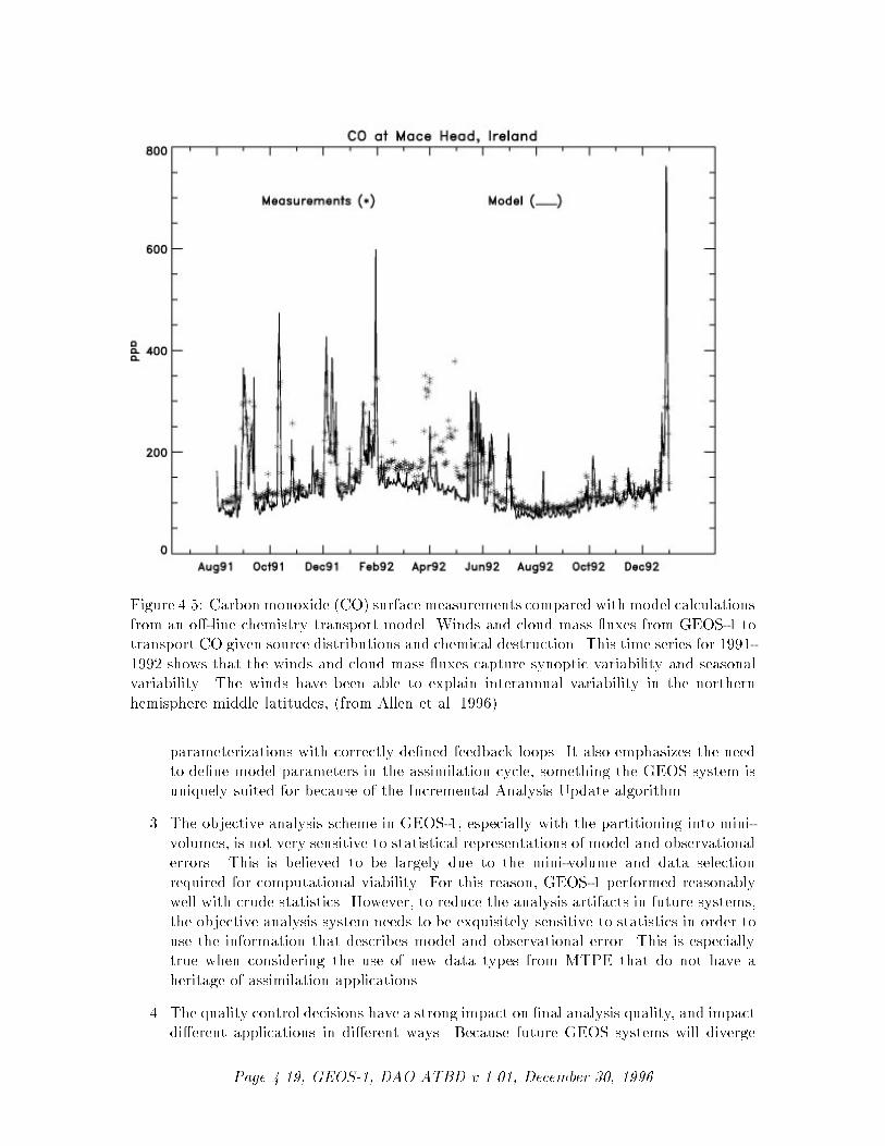
Figure 4.5: Carbon monoxide (CO) surface measurements compared with model calculations
from an o�-line chemistry transport model. Winds and cloud mass uxes from GEOS-1 to
transport CO given source distributions and chemical destruction. This time series for 1991-
1992 shows that the winds and cloud mass uxes capture synoptic variability and seasonal
variability. The winds have been able to explain interannual variability in the northern
hemisphere middle latitudes, (from Allen et al. 1996).
parameterizations with correctly de�ned feedback loops. It also emphasizes the need
to de�ne model parameters in the assimilation cycle, something the GEOS system is
uniquely suited for because of the Incremental Analysis Update algorithm.
3. The objective analysis scheme in GEOS-1, especially with the partitioning into mini-
volumes, is not very sensitive to statistical representations of model and observational
errors. This is believed to be largely due to the mini-volume and data selection
required for computational viability. For this reason, GEOS-1 performed reasonably
well with crude statistics. However, to reduce the analysis artifacts in future systems,
the objective analysis system needs to be exquisitely sensitive to statistics in order to
use the information that describes model and observational error. This is especially
true when considering the use of new data types from MTPE that do not have a
heritage of assimilation applications.
4. The quality control decisions have a strong impact on �nal analysis quality, and impact
di�erent applications in di�erent ways. Because future GEOS systems will diverge
Page 4.19, GEOS-1, DAO ATBD v 1.01, December 30, 1996

from numerical weather prediction assimilation systems, reliance on NCEP quality
control is short-sighted. This is especially true when new data types are considered.
5. Evaluation of long-term assimilated data sets with parallel model integrations is a
powerful way to understand system performance. Preconceived ideas that the model
and assimilation would be so closely intertwined as to defy de�nitive identi�cation
of problems are found to be untrue. In fact, Chen et al. (1996) �nd that a parallel
integration with a di�erent model often compares better with the GEOS-1 assimilation
than does the GEOS-1 GCM. As a model validation technique, the comparison of
parallel simulations and assimilations, help to bridge the gap between integrated and
process oriented model diagnostics.
6. Model forecasts have been underutilized in the GEOS development strategy. Despite
relatively low resolution, the current GEOS GCM can provide numerical weather fore-
casts that only trail the operational forecast skill scores for the northern hemisphere
winter by approximately half a day at seven days. However, the GEOS model falls
behind in the �rst 48 hours of the forecast. The lack of predictability on the shortest
time scales implies that information propagation is not as good as it should be (Fourth
Report of the DAO Science Advisory Panel).
7. The ability of the assimilated data to advance quantitative science might be more
dependent on post-processing algorithms than previously thought. Interpolation rou-
tines and output strategies strongly impact the ability to calculate closed budgets
of tracers, heat, momentum or energy from archived data sets. The impact of third
party post-processing and subsetting tools must be evaluated.
8. There are many potential bottlenecks in the production stream. Some of the most
di�cult have been related to �nding historical data and performing basic quality
control on these data sets. In addition, the interaction of computers in a distributed
production environment requires the development of new types of backup capabilities
to assure operational production.
Page 4.20, GEOS-1, DAO ATBD v 1.01, December 30, 1996
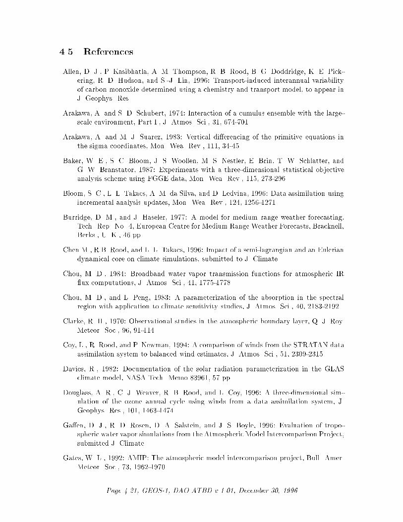
4.5 References
Allen, D. J., P. Kasibhatla, A. M. Thompson, R. B. Rood, B. G. Doddridge, K. E. Pick-
ering, R. D. Hudson, and S.-J. Lin, 1996: Transport-induced interannual variability
of carbon monoxide determined using a chemistry and transport model, to appear in
J. Geophys. Res.
Arakawa, A. and S. D. Schubert, 1974: Interaction of a cumulus ensemble with the large-
scale environment, Part I., J. Atmos. Sci., 31, 674-701.
Arakawa, A. and M. J. Suarez, 1983: Vertical di�erencing of the primitive equations in
the sigma coordinates, Mon. Wea. Rev., 111, 34-45.
Baker, W. E., S. C. Bloom, J. S. Woollen, M. S. Nestler, E. Brin, T. W. Schlatter, and
G. W. Branstator, 1987: Experiments with a three-dimensional statistical objective
analysis scheme using FGGE data, Mon. Wea. Rev., 115, 273-296.
Bloom, S. C., L. L. Takacs, A. M. da Silva, and D. Ledvina, 1996: Data assimilation using
incremental analysis updates, Mon. Wea. Rev., 124, 1256-1271.
Burridge, D. M., and J. Haseler, 1977: A model for medium range weather forecasting,
Tech. Rep. No. 4, European Centre for Medium Range Weather Forecasts, Bracknell,
Berks., U. K., 46 pp.
Chen M., R.B. Rood, and L. L. Takacs, 1996: Impact of a semi-lagrangian and an Eulerian
dynamical core on climate simulations, submitted to J. Climate.
Chou, M. D., 1984: Broadband water vapor transmission functions for atmospheric IR
ux computations, J. Atmos. Sci., 41, 1775-1778.
Chou, M. D., and L. Peng, 1983: A parameterization of the absorption in the spectral
region with application to climate sensitivity studies, J. Atmos. Sci., 40, 2183-2192.
Clarke, R. H., 1970: Observational studies in the atmospheric boundary layer, Q. J. Roy.
Meteor. Soc., 96, 91-114.
Coy, L., R. Rood, and P. Newman, 1994: A comparison of winds from the STRATAN data
assimilation system to balanced wind estimates, J. Atmos. Sci., 51, 2309-2315.
Davies, R., 1982: Documentation of the solar radiation parameterization in the GLAS
climate model, NASA Tech. Memo 83961, 57 pp.
Douglass, A. R., C. J. Weaver, R. B. Rood, and L. Coy, 1996: A three-dimensional sim-
ulation of the ozone annual cycle using winds from a data assimilation system, J.
Geophys. Res., 101, 1463-1474.
Ga�en, D. J., R. D. Rosen, D. A. Salstein, and J. S. Boyle, 1996: Evaluation of tropo-
spheric water vapor simulations from the Atmospheric Model Intercomparison Project,
submitted J. Climate.
Gates, W. L., 1992: AMIP: The atmospheric model intercomparison project, Bull. Amer.
Meteor. Soc., 73, 1962-1970.
Page 4.21, GEOS-1, DAO ATBD v 1.01, December 30, 1996

Harrison, E. F., P. Minnis, B. R. Barkstrom, V. Ramanathan, R. D. Cess, and G. G.
Gibson, 1990: Seasonal variation of cloud radiative forcing derived from the Earth
Radiation Budget Experiment, J. Geophys. Res., 95, 18687-18703.
Harshvardhan, R. Davies, D. A. Randall, and T. G. Coresetti, 1987: A fast radiation
parameterization for atmospheric general circulation models, J. Geophys. Res., 92,
1009- 1016.
Helfand, H. M., and J. C. Labraga, 1988: Design of a non-singular level 2.5 second-order
closure model for the prediction of atmospheric turbulence, J. Atmos. Sci., 45, 113-
132.
Helfand, H. M., M. Fox-Rabinovitz, L. Takacs, and A, Molod, 1991: Simulation of the
planetary boundary layer and turbulence in the GLA GCM, Proc. AMS Ninth Conf.
on Numerical Weather Prediction, Denver, CO.
Helfand, H. M., and S. D. Schubert, 1995: Climatology of the simulated Great Plains low-
level jet and its contribution to the continental moisture budget of the United States,
J. Climate, 784-806.
Joseph, J. H., W. J. Wiscombe, and J. E. Weinman, 1976: The delta-Eddington approxi-
mation for radiative ux transfer, J. Atmos. Sci., 33, 2452-2459.
King, M. D., and Harshvardhan, 1986: Comparative accuracy of selected multiple scatter-
ing approximations, J. Atmos. Sci., 43, 784-801.
Lacis, A. A., and J. E. Hansen, 1974: A parameterization for the absorption of solar
radiation in the Earth's atmosphere, J. Atmos. Sci., 31, 118-133.
Lau, K.-M., J. H. Kim, and Y. Sud, 1996: Intercomparison of hydrologic processes in
AMIP GCMs, Bull. Amer. Meteor. Soc., 77, 2209-2227.
Legates, D. R., and C. J. Wilmott, 1990: Mean seasonal and spatial variability in gage-
corrected global precipitation, Int. J. Climate, 10, 111-127.
Min, W., and S. D. Schubert, 1996: The climate signal in regional moisture uxes: a
comparison of three global data assimilation products, submitted J. Climate.
Molod, A., H. M. Helfand, L. L. Takacs, 1996: The climatology of parameterized physical
processes in the GEOS-1 GCM and their impact on the GEOS-1 Data Assimilation
System, J. Climate, 9, 764-785.
Panofsky, H. A., 1973: Tower micrometeorology. In Workshop on Micrometeorology, D.
A. Haugen (ed.), American Meteorological Society, Boston, 392 pp.
Park, C.-K, and S. D. Schubert, 1996: On the nature of the 1994 East Asian summer
drought, to appear J. Climate.
Pfaendtner, J., S. Bloom, D. Lamich, M. Seablom, M. Sienkiewicz, J. Stobie, A. da Silva,
1995: Documentation of the Goddard Earth Observing System (GEOS) Data Assim-
ilation System-Version 1, NASA Tech. Memo. No. 104606, Vol. 4, Goddard Space
Flight Center, Greenbelt, MD 20771.
Page 4.22, GEOS-1, DAO ATBD v 1.01, December 30, 1996

Rodgers, C. D., 1968: Some extensions and applications of the new random model for
molecular band transmission, Q. J. Roy. Meteor. Soc., 94, 99-102.
Rood, R. B., A. R. Douglass, J. A. Kaye, M. A. Geller, Y. Chi, D. J. Allen, E. M. Larson,
E. R. Nash, and J. E. Nielsen, 1991: Three-dimensional simulations of wintertime
ozone variability in the lower stratosphere, J. Geophys. Res., 96, 5055-5071.
Rosen�eld, J. E., M. R. Schoeberl, and M. A. Geller, 1987: A computation of the strato-
spheric diabatic circulation using an accurate radiative transfer model, J. Atmos. Sci.,
44, 859-876.
Rossow, W. L, and R. A. Schi�er, 1991: ISCCP cloud data products, Bull. Amer. Meteor.
Soc., 72, 2-21.
Sadourney, R., 1975: The dynamics of �nite di�erence models of the shallow water equa-
tions, J. Atmos. Sci., 32, 680-689.
Schubert, S., C.-K. Park, Chung-Yu Wu, W. Higgins, Y. Kondratyeva, A. Molod, L.
Takacs, M. Seablom, and R. Rood, 1995: A Multiyear Assimilation with the GEOS-1
System: Overview and Results, NASA Tech. Memo. 104606, Vol. 6, Goddard Space
Flight Center, Greenbelt, MD 20771.
Schubert, S. D. and R. Rood, 1995: Proceedings of the Workshop on the GEOS-1 Five-
Year Assimilation, NASA Tech. Memo. 104606, Vol. 7, Goddard Space Flight Center,
Greenbelt, MD 20771.
Seablom, M. S., J. W. Pfaendtner, and P. E. Piraino, 1991: Quality control techniques for
the interactive GLA retrieval/assimilation system, preprint volume, Ninth Conf. on
Numerical Weather Prediction, Amer. Meteor. Soc., 28-29.
Sud, Y., and A. Molod, 1988: The roles of dry convection, cloud-radiation feedback pro-
cesses and the in uences of recent improvements in the parameterization of convection
in the GLA AGCM, Mon. Wea. Rev., 116, 2366-2387.
Takacs, L., A. Molod and T. Wang, 1994: Documentation of the Goddard Earth Observing
System (GEOS) General Circulation Model -Version 1, NASA Tech. Memo. 104606,
Vol. 1.
Weare, B. C., I. I. Mokhov, and Project Members, 1995: Evaluation of total cloudiness
and its variability in the Atmospheric Model Intercomparison Project, J. Climate, 8,
2224- 2238.
Page 4.23, GEOS-1, DAO ATBD v 1.01, December 30, 1996

4.6 Acronyms
4.6.1 General acronyms
DAO Data Assimilation O�ce
GEOS Goddard Earth Observing System (The name of the DAO
data assimilation system)
GCM General Circulation Model
DAS Data Assimilation System
QC Quality Control
NWP Numerical Weather Prediction
CARD Consistent Assimilation of Retrieved Data
PSAS Physical-space Statistical Analysis System
NASA National Aeronautics and Space Administration
GSFC Goddard Space Flight Center
MTPE Mission to Planet Earth
EOS Earth Observing System
EOSDIS Earth Observing System Data and Information System
NOAA National Oceanic and Atmospheric Administration
NCEP National Centers for Environmental Prediction (formerly, NMC)
NMC National Meteorological Center
NESDIS National Environmental Satellite Data and Information Service
ECMWF European Center for Medium-range Weather Forecasts
UKMO United Kingdom Meteorological O�ce
4.6.2 Instruments
ADEOS Advanced Earth Observting Satellite (Mid-late 1996)
AIRS Atmospheric Infrared Sounder (EOS PM)
AMSU A-B Advanced Microwave Sounding Unit (POES, EOS PM)
AVHRR Advanced Very High-Resolution Radiometer
ASTER Advanced Spaceborne Thermal Emission and Re ection
Radiometer (EOS AM)
ATOVS Advanced TOVS; HIRS3/AMSU (POES)
CERES Clouds and Earth's Radiation Energy System (TRMM, EOS AM)
CLAES Cryogenic Limb Array Etalon Spectrometer (UARS)
DMSP Defense Meteorological Satellite Program (currently operational)
EOS AM1 Earth Observting Satellite AM (June 98 launch)
EPS EUMETSAT (European Meteorology Satellite) Polar System
ERBE Earth Radiation Budget Experiment (ERBS)
ERBS Earth Radiation Budget Satellite
ERS-1,2 European Remote Sensing Satellite (Scatterometer,
6 channel, IR-Visible radiometer)
Page 4.24, GEOS-1, DAO ATBD v 1.01, December 30, 1996
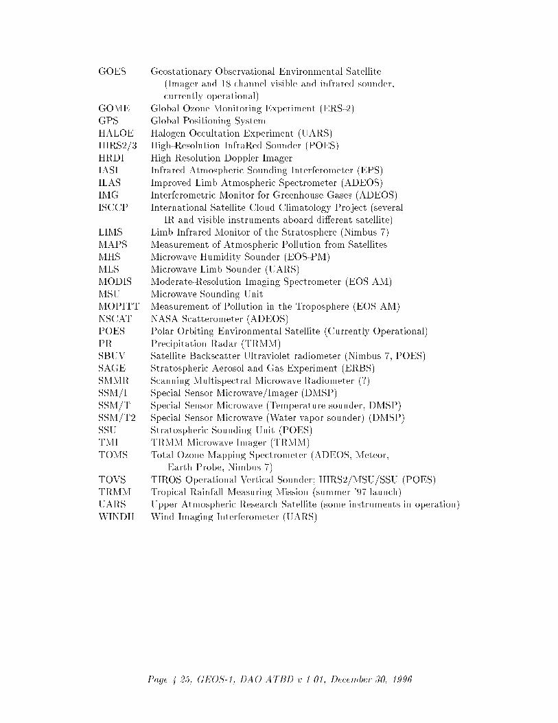
GOES Geostationary Observational Environmental Satellite
(Imager and 18 channel visible and infrared sounder,
currently operational)
GOME Global Ozone Monitoring Experiment (ERS-2)
GPS Global Positioning System
HALOE Halogen Occultation Experiment (UARS)
HIRS2/3 High-Resolution InfraRed Sounder (POES)
HRDI High Resolution Doppler Imager
IASI Infrared Atmospheric Sounding Interferometer (EPS)
ILAS Improved Limb Atmospheric Spectrometer (ADEOS)
IMG Interferometric Monitor for Greenhouse Gases (ADEOS)
ISCCP International Satellite Cloud Climatology Project (several
IR and visible instruments aboard di�erent satellite)
LIMS Limb Infrared Monitor of the Stratosphere (Nimbus 7)
MAPS Measurement of Atmospheric Pollution from Satellites
MHS Microwave Humidity Sounder (EOS-PM)
MLS Microwave Limb Sounder (UARS)
MODIS Moderate-Resolution Imaging Spectrometer (EOS AM)
MSU Microwave Sounding Unit
MOPITT Measurement of Pollution in the Troposphere (EOS AM)
NSCAT NASA Scatterometer (ADEOS)
POES Polar Orbiting Environmental Satellite (Currently Operational)
PR Precipitation Radar (TRMM)
SBUV Satellite Backscatter Ultraviolet radiometer (Nimbus 7, POES)
SAGE Stratospheric Aerosol and Gas Experiment (ERBS)
SMMR Scanning Multispectral Microwave Radiometer (?)
SSM/I Special Sensor Microwave/Imager (DMSP)
SSM/T Special Sensor Microwave (Temperature sounder, DMSP)
SSM/T2 Special Sensor Microwave (Water vapor sounder) (DMSP)
SSU Stratospheric Sounding Unit (POES)
TMI TRMM Microwave Imager (TRMM)
TOMS Total Ozone Mapping Spectrometer (ADEOS, Meteor,
Earth Probe, Nimbus 7)
TOVS TIROS Operational Vertical Sounder; HIRS2/MSU/SSU (POES)
TRMM Tropical Rainfall Measuring Mission (summer '97 launch)
UARS Upper Atmospheric Research Satellite (some instruments in operation)
WINDII Wind Imaging Interferometer (UARS)
Page 4.25, GEOS-1, DAO ATBD v 1.01, December 30, 1996
Chapter 5
The Goddard EarthObserving System { Version 2Data Assimilation System(GEOS-2 DAS)
Contents
5.1 Overview of the Data Assimilation Algorithm . . . . . . . . . . 5.2
5.2 The Physical-space Statistical Analysis System (PSAS) . . . . 5.3
5.2.1 Design objectives . . . . . . . . . . . . . . . . . . . . . . . . . . . . 5.3
5.2.2 Background: the statistical analysis equations . . . . . . . . . . . . 5.4
5.2.3 The global PSAS solver . . . . . . . . . . . . . . . . . . . . . . . . 5.5
5.2.4 Di�erences between PSAS, OI and spectral variational schemes . . 5.8
5.2.5 Comparison of the global PSAS solver with the localized OI solver 5.12
5.2.6 The analysis equations in the presence of forecast bias . . . . . . . 5.17
5.2.7 Speci�cation of error statistics . . . . . . . . . . . . . . . . . . . . 5.19
5.3 The GEOS-2 General Circulation Model . . . . . . . . . . . . . 5.33
5.3.1 Introduction and Model Lineage . . . . . . . . . . . . . . . . . . . 5.33
5.3.2 Atmospheric Dynamics . . . . . . . . . . . . . . . . . . . . . . . . 5.34
5.3.3 Atmospheric Physics . . . . . . . . . . . . . . . . . . . . . . . . . . 5.48
5.3.4 Boundary Conditions and other Input Data . . . . . . . . . . . . . 5.60
5.4 Combining model and analysis: the IAU process . . . . . . . . 5.68
5.4.1 Filtering properties of IAU . . . . . . . . . . . . . . . . . . . . . . 5.70
5.4.2 Impact of IAU on GEOS-1 DAS . . . . . . . . . . . . . . . . . . . 5.72
5.4.3 Model/analysis interface . . . . . . . . . . . . . . . . . . . . . . . . 5.72
5.5 References . . . . . . . . . . . . . . . . . . . . . . . . . . . . . . . . 5.75
5.6 Acronyms . . . . . . . . . . . . . . . . . . . . . . . . . . . . . . . . 5.81
5.6.1 General acronyms . . . . . . . . . . . . . . . . . . . . . . . . . . . 5.81
5.6.2 Instruments . . . . . . . . . . . . . . . . . . . . . . . . . . . . . . . 5.81
Page 5.1, GEOS-2 DAS, DAO ATBD v 1.01, December 30, 1996

5.1 Overview of the Data Assimilation Algorithm
This Chapter and the following two chapters on Quality Control and New Data Types
describe the core capabilities of the GEOS-2 Data Assimilation System (DAS). The basic
components of the GEOS DAS were described in section 2.2 and a schematic of the system
was given in Figure 2.1. The major components of the system were identi�ed as the sta-
tistical objective analysis, the model, and the quality control algorithm. In addition it was
noted that there are major tasks to develop forecast and observational error statistics for
the objective analysis and to develop boundary conditions for the model. In this chapter the
objective analysis and the model are discussed, along with the e�orts to develop improved
statistics and boundary conditions.
The GEOS-2 Physical-space Statistical Analysis System (PSAS) is an entirely new al-
gorithm. It is a state-of-the-art system, with the versatility and capability to accommo-
date future developments in data assimilation methodology in a manner consistent with
estimation theory. The DAO Advisory Panel identi�ed the successful development and
implementation of PSAS as crucial to the success of the GEOS system. The DAO Plan
(1994-2000) identi�ed the ambitious development of PSAS as one of four high-risk activities.
This chapter will show that many major hurdles in developing PSAS have been overcome.
The current GEOS-2 validation exercises are demonstrating the successful implementation
of PSAS.
The GEOS-2 General Circulation Model (GCM) is an incremental development over
GEOS-1. The model description includes several developments that are aimed at addressing
speci�c problems discovered in GEOS-1. In addition, the model has been prepared for
broader future capabilities to meet the science requirements and scope outlined in Chapter 2.
Both the analysis and the model have been designed to accommodate new data types.
This includes the ability to implement arbitrary observation operators in the analysis and
to generalize the speci�cation of error statistics. The model design incorporates more
physically-based parameterizations, including the introduction of new variables that im-
prove the link to the expanded observation suite. A major model development to follow
GEOS-2 is the inclusion of an interactive land-surface model. Many aspects of GEOS-2
provide the foundation for the integration of the land-surface model. The incorporation
of new data types is discussed extensively in Chapter 7. Development beyond GEOS-2 is
discussed in Chapter 9.
The development detailed here follows from the GEOS-1 project in many ways. The
lessons learned from GEOS-1 (see Chapter 4) are either explicitly or implicitly addressed
in the GEOS-2 development. In some ways the development is aimed at meeting a base-
line credibility requirement for the GEOS DAS. More broadly, the development builds the
infrastructure to anticipate future requirements as Earth science and the data assimilation
mission evolve. Developments that are directed at solving explicit shortcomings identi�ed
in the GEOS-1 data sets and their applications are aimed as much as possible at improving
the underlying physics of the model or the statistical basis of the analysis system. Fixes
targeting speci�c problems are avoided as much as possible.
Page 5.2, GEOS-2 DAS, DAO ATBD v 1.01, December 30, 1996

5.2 The Physical-space Statistical Analysis System (PSAS)
5.2.1 Design objectives
At the time the DAO was formed, in February 1992, plans were initiated to develop a new
statistical analysis system called the Physical-space Statistical Analysis System (PSAS).
PSAS was designed to meet the following �ve requirements.
1. To establish and remove the e�ects of data selection in the GEOS-1 optimal interpo-
lation (OI) system. This objective requires PSAS to be capable of using forecast and
observation error covariance models identical to those speci�ed in the OI system, but
to solve the analysis equations globally rather than locally.
2. To obtain proper sensitivity to all data and to all error covariance speci�cations.
In Baker et al. (1987), for instance, it was shown that introducing geographically-
dependent forecast error covariances had little impact on OI analyses. It is likely that
global solution of the analysis equations demanded by objective (1) would reveal much
more robust responsiveness, forcing one to pay careful attention to error covariance
formulations. Recent experiments with the PSAS system (not described here) have
in fact demonstrated strong sensitivity to these formulations and will be described in
future publications.
3. To permit assimilation of new data types that are not state variables. A great wealth of
data, mostly from space-borne remote-sensing devices, will become available in coming
years. Data selection would become an increasingly onerous and ad hoc procedure for
these data. More importantly, many of these data, especially if assimilated in raw form
(e.g., radiances or backscatter) rather than as retrieved products, are neither state
variables nor linearly related to state variables. While some types of data that are not
state variables, such as total precipitable water, have been successfully assimilated
with the OI methodology (Ledvina and Pfaendtner 1995), global formulation of the
analysis problem, in which observation operators are de�ned explicitly, provides a
natural framework for assimilating these data types (e.g., Eyre et al. 1993, Derber
and Wu 1996, Joiner and da Silva 1996). The version of PSAS described in this
Chapter incorporates linear (i.e., state-independent) observation operators only. A
version of the PSAS algorithm for nonlinear observation operators is described in
Chapter 9 (see also Cohn 1996, section 5).
4. To allow maximum exibility in forecast and observation error covariance modeling.
While much e�ort has been directed toward covariance modeling in recent years, it is
likely that additional e�orts will result in improved analyses. For instance, while global
spectral analysis systems rely explicitly on an assumption that forecast errors are
horizontally isotropic, it is well-known (e.g., Courtier et al. 1994, Th�epaut et al. 1996,
Cohn and Todling 1996 and references therein) that these errors are in fact highly
anisotropic. Although the �rst implementation of GEOS-2 does not take advantage
of this capability, much of the GEOS-3 development is focused on improved error
statistics. The development of anisotropic correlation modeling in PSAS is discussed
in Chapter 9.
Page 5.3, GEOS-2 DAS, DAO ATBD v 1.01, December 30, 1996

5. To enable exibility for future developments in data assimilation methodology. The
PSAS system was envisioned from the outset to provide a computational framework
for the development of techniques for �xed-lag Kalman smoothing (Todling et al. 1996,
Cohn et al. 1994), approximate Kalman �ltering (e.g., Cohn and Todling 1996), fore-
cast bias estimation (Dee and da Silva 1996), and other topics known from the es-
timation theory literature but not yet implemented in operational data assimilation
systems (see Chapter 9). Solution of the innovation covariance equation, a key compo-
nent of the PSAS system described below, is a need common to all of these techniques.
Because of these design features PSAS has the following attributes:
a. PSAS solves the analysis equations globally rather than locally. The local approxima-
tion and data selection of OI schemes is eliminated. In this respect, PSAS is similar to
the global variational spectral analysis systems that have recently replaced OI schemes
at NCEP (Parrish and Derber 1992) and at ECMWF (Heckley et al. 1993, Courtier
et al. 1993).
b. PSAS works directly in physical space, like OI schemes but unlike spectral analysis
schemes.
c. PSAS performs a large part of its calculations in observation space, also unlike op-
erational spectral analysis schemes, which operate in state space. This results in
computational savings, since the dimension of the observation space is currently an
order of magnitude smaller than that of the forecast model state. The computational
e�ciency of spectral analysis schemes arises from an assumption that horizontal fore-
cast error covariances or correlations are isotropic, i.e., diagonal in spectral space, an
assumption which is not made in the PSAS algorithm.
d. PSAS is fundamentally independent of the model formulation, and hence, is a portable
algorithm suitable for many applications. While compatible with the grid-point sys-
tem of the GEOS GCM, nothing in the design restricts PSAS applications to this
grid. In particular PSAS is suitable for regional assimilation and problems on irregu-
lar grids.
5.2.2 Background: the statistical analysis equations
A statistical analysis scheme attempts to obtain an optimal estimate, or analysis, of the state
of the system by combining observations with a forecast model �rst guess. Let wf 2 IRn
denote the vector representing the forecast �rst guess, de�ned on a grid in our case, and let
wt 2 IRn denote the true state approximated by wf ,
wf = wt + �f ; (5.1)
where �f 2 IRn denotes the forecast error. Let wo 2 IRp denote the vector of p observationsavailable at the analysis time, assumed to be related linearly to the state variables,
wo = Hwt + �o: (5.2)
Page 5.4, GEOS-2 DAS, DAO ATBD v 1.01, December 30, 1996

Here H 2 IRp � IRn is the observation operator, or generalized interpolation operator;
�o 2 IRp denotes the observation error, which is the sum of the measurement error and the
error of representativeness (e.g., Cohn 1996). Currently the number of model degrees of
freedom is n � 106 and the current observing system has p � 105.
The probabilistic assumptions common to most operational analysis systems are that
�f and �o are Gaussian-distributed with zero mean, and are not correlated with either the
state or with each other. While these assumptions can be relaxed in a variety of ways (cf.
Cohn 1996 and references therein), the current implementation of PSAS invokes all of them.
E�orts directed toward relaxing the assumption that �f has zero mean�D�fE= 0
�, that is,
that the forecast is unbiased, are described in section 5.2.6 and in Chapter 9.
The two most common optimality criteria, arising from minimum variance estimation
and maximum likelihood estimation, lead to identical analysis equations under these as-
sumptions (e.g., Lorenc 1986, Cohn 1996). These equations also yield the best linear un-
biased estimate (BLUE), or analysis, without an assumption that the errors �f and �o are
Gaussian-distributed.
Theminimum variance analysis wa 2 IRn is obtained by requiringD�wa � wt
�TS�wa � wt
�Eto be minimum for all positive de�nite matrices S 2 IRn � IRn, and under the stated as-
sumptions is given by the analysis equations
wa = wf +K�wo �Hwf
�(5.3)
K = P fHT�HP fHT +R
��1: (5.4)
Here the matrix K is the gain matrix, which ascribes appropriate weights to the observa-
tions. The gain matrix depends on the forecast error covariance matrix
P f ����f �
D�fE��
�f �D�fE�T�
2 IRn � IRn (5.5)
and on the observation error covariance matrix
R �D(�o � h�oi) (�o � h�oi)T
E2 IRp � IRp: (5.6)
Both are symmetric and positive semi-de�nite by de�nition; R is in fact positive de�nite
under an assumption that no linear combination of the observations is perfect. While these
matrices are de�ned as above, in practice they must be modeled. The modeling strategy of
PSAS for GEOS-2 is detailed in section 5.2.7.
5.2.3 The global PSAS solver
The PSAS algorithm solves the analysis equations in a straightforward manner. First, one
p� p linear system is solved for the quantity y,
�HP fHT + R
�y = wo �Hwf ; (5.7)
Page 5.5, GEOS-2 DAS, DAO ATBD v 1.01, December 30, 1996

and then the analyzed state wa is obtained from the equation
wa = wf + P fHTy: (5.8)
Equations (5.7) and (5.8) will be referred to as the PSAS equations. The innovation co-
variance matrix
M � HP fHT + R (5.9)
is symmetric positive de�nite, making a standard pre-conditioned conjugate gradient (CG)
algorithm (Golub and van Loan 1989) the method of choice for solving the large linear sys-
tem (5.7). For the current observing system, setting up and solving the linear system (5.7)
costs about half the computational e�ort of PSAS, and involves computation in observation
space: M 2 IRp � IRp and y 2 IRp. The other half of the computational expense is taken
by step (5.8) which transfers the solution y to the state space: P fHTy 2 IRn.The GEOS-2 version of PSAS analyzes global sea level pressure and near surface winds
over the oceans, as well as geopotential height, vector wind, and water vapor mixing ratio
on constant pressure surfaces. The upper air height/wind analyses and the sea level pres-
sure/surface wind analyses are multivariate using the wind-mass error covariance models
described in subsection 5.2.7. The moisture analysis is done with a univariate statistical
algorithm, and only at levels from 1000 hPa to 300 hPa. The basic GEOS-2 DAS con�gu-
ration consists of a 2� latitude by 2:5� longitude, and 18 vertical levels (0.4, 1, 5, 7, 10, 30,
50, 70, 100, 150, 200, 250, 300, 400, 500, 700, 850, 1000 hPa). Details of the model/analysis
interface are given in subsection 5.4.3.
For typical models of P f and R the innovation covariance matrix M is not sparse,
although entries associated with remote pairs of observation locations are negligibly small.
To introduce some sparseness in M and thereby to save computational e�ort, the sphere is
divided into N regions, and matrix blocks associated with regions separated by more than
6,000 km are assumed to be zero; these blocks never enter the CG computations. The same
procedure is applied to the matrix P f itself in (5.8). While this procedure could in principle
destroy the positive-de�niteness of M , causing lack of convergence of the CG solver, this
has not been observed in the experiments reported in section 5.2.5 using the covariance
models P f and R of the GEOS-1 OI system. A rigorous approach based on space-limited
covariance models (Gaspari and Cohn 1996), which are exactly zero beyond a speci�ed
distance, is used in GEOS-2, as described in section 5.2.7.
A good pre-conditioner for the CG algorithm must have two important characteristics:
1) it must be inexpensive to compute, and 2) it must retain the essentials of the original
problem if it is to e�ectively improve the convergence rate of the algorithm. For the statis-
tical interpolation problem that PSAS implements, a natural candidate for pre-conditioner
is an OI-like approximation, in which the problem is solved separately for each of the N
regions used to partition the data. For the Cray C-90 implementation the globe is divided
into 80 equal-area regions using an icosahedral grid (Pfaendtner 1996) 1. With p � 100; 000
observations and N � 80 regions, each of these regional problems have on average more
1In the massively parallel implementation of PSAS being developed at JPL the globe is divided in 256
or 512 geographically irregular regions, each having approximately the same number of observations. This
strategy is necessary to achieve load balance (Ding and Ferraro 1996).
Page 5.6, GEOS-2 DAS, DAO ATBD v 1.01, December 30, 1996

Recursive
Preconditioned
Conjugate Gradient Solver
PSAS
CONJGR
CONJGR2
CONJGR1
SPPTRF + SPPTRS
full matrix
regional diagonal
univariate diagonal
profiles diagonal
cg_main( )
cg_level2( )
cg_level1( )
Conjugate Gradient SolverNested Pre-conditioned
PSAS
Figure 5.1: PSAS nested pre-conditioned conjugate gradient solver. Routine cg main() containsthe main conjugate gradient driver. This routine is pre-conditioned by cg level2(), which solvesa similar problem for each region. This routine is in turn pre-conditioned by cg level1() whichsolves the linear system univariately. See text for details.
than 1,000 observations, too many for an e�cient pre-conditioner. These regional problems
are therefore solved by another pre-conditioned conjugate gradient algorithm; we refer to
this solver as the CG level 2. As a pre-conditioner for CG level 2 the same problem is
solved univariately for each data type, i.e., observations of u-wind, v-wind, geopotential
height, etc., are treated in isolation. However, these univariate problems are still too large
to be e�ciently solved by direct methods and yet another iterative solver is used; this is
the CG level 1 algorithm. As a pre-conditioner for CG level 1 we make use of LAPACK
(Anderson et al. 1992) to perform a direct Cholesky factorization of diagonal blocks of
the level 1 correlation sub-matrix. These diagonal blocks are typically of size 32, and are
carefully chosen to include full vertical pro�les, a desirable feature for the implementation
of new data types. These nested pre-conditioned conjugate gradient solvers are illustrated
in Figure 5.1. Additional details about the pre-conditioner can be found in da Silva and
Guo (1996).
In the current serial implementation of PSAS, the matrix M is �rst normalized by its
main diagonal, the normalized matrix is provided to the global CG solver as an operator,
and the matrix elements are recomputed each CG iteration. In the parallel implementation
of PSAS being developed at the Jet Propulsion Laboratory (Ding and Ferraro 1996), blocks
of the matrix M are pre-computed and stored in memory. As a convergence criterion for
the CG solver we specify that the residual must be reduced by 1 or 2 orders of magni-
Page 5.7, GEOS-2 DAS, DAO ATBD v 1.01, December 30, 1996

tude. Experiments with reduction of the residual beyond 2 orders of magnitude produced
di�erences much smaller than expected analysis errors. This is mainly due to the �ltering
properties of the operator P fHT in (5.8), which attenuates the small-scale details in the
linear system variable y.
5.2.4 Di�erences between PSAS, OI and spectral variational schemes
In this subsection we discuss the main distinctions between the PSAS approach to solving
the analysis equations (5.3), (5.4), the approach of OI schemes, and the approach of spectral
variational schemes.
Optimal interpolation schemes solve equations (5.3){(5.4) approximately, as follows.
Denote by kj the jth column of the transposed gain matrix KT de�ned by (5.4), so that
kj 2 IRp. Then (5.4) can be written as
�HP fHT + R
�kj = (HP f )j (5.10)
for j = 1; : : : ; n, where (HP f)j 2 IRp denotes the jth column of the matrix HP f . This
equation represents n linear systems, each of the same form as the PSAS equation (5.7).
Similarly, equation (5.3) can be written as n scalar equations,
waj = wfj + (kj)
T�wo �Hwf
�(5.11)
for j = 1; : : : ; n, where waj and wfj denote the jth elements of wa and wf , respectively.
This equation makes it clear that the weight vector kj solved for in (5.10) determines the
correction, or analysis increment, at the jth grid point.
Equations (5.10) and (5.11) would yield the same analysis wa as the PSAS equations
(5.7) and (5.8), but at far greater computational expense since there are n linear systems
to be solved in (5.10) but only one in (5.7). Optimal interpolation schemes do in fact solve
(5.10) and (5.11), but with a local approximation and hence the need for data selection.
These schemes di�er widely in the details of the local approximation and the data selection
algorithm (cf. McPherson et al. 1979; Lorenc 1981; Baker et al. 1987; Pfaendtner et al.
1995), but all can be described in a generic way as follows.
Instead of involving all p observations in the solution of each of the j equations (5.10) and
(5.11), some much smaller number q of observations nearby the jth grid location is selected
for the analysis at that location, and a di�erent subset of observations, q = q(j), is selected
for di�erent locations j. [In the GEOS-1 OI system, q = 75 and a �xed subset of observations
is selected for a given mini-volume.] Thus wo, H , and R become lower-dimensional and are
made to depend on the grid-point index j: wo = woj 2 IRq, H = Hj 2 IRq � IRn, and
R = Rj 2 IRq � IRq. [This is a slight abuse of notation; for these quantities the subscript j
simply denotes dependence on the grid-point index, while otherwise it denotes a column of
a matrix or an element of a vector.] Thus in OI schemes the analysis equations (5.10) and
(5.11) can be written as
�HjP
fHTj +Rj
�kj =
�HjP
f�j
(5.12)
Page 5.8, GEOS-2 DAS, DAO ATBD v 1.01, December 30, 1996
and
waj = wfj + (kj)
T�woj �Hjw
f�
(5.13)
for j = 1; : : : ; n, where now kj 2 IRq. While there are still n systems to solve in (5.12),
each is now only q� q (this is the local approximation), and q is small enough that a direct
method such as the standard Cholesky algorithm can be used to solve them. In addition,
the matrix Mj = HjPfHT
j + Rj in (5.12) itself is �xed for a given volume, so that the
Cholesky decomposition can be re-used for each grid point j in a given volume, reducing
computational e�ort.
An important distinction between OI schemes and the PSAS scheme is that the weights
kj themselves are solved for in (5.12), albeit approximately, rather than the vector y in (5.7).
This gives OI schemes the ability to calculate approximately the analysis error variances
in the following simple fashion. Under the same probabilistic assumptions noted above
equation (5.3), the analysis error covariance matrix
P a �D(�a � h�ai) (�a � h�ai)T
E2 IRn � IRn; (5.14)
where
�a = wa � wt (5.15)
is the analysis error, is given by
P a = P f �KHP f ; (5.16)
whose (i; j)th element is
P aij = Pfij � (ki)
T�HP f
�j: (5.17)
The diagonal elements P ajj , or analysis error variances, are then
P ajj = Pfjj � (kj)
T�HP f
�j; (5.18)
which under the local approximation becomes
P ajj = Pfjj � (kj)
T�HjP
f�j: (5.19)
The ingredients for this simple computation are available from equation (5.12). A similar
computation could be carried out at small additional cost in the PSAS algorithm at CG
level 2, but has not been implemented at present. This would have the desirable e�ect
of overestimating the analysis error variances, since not all of the data would enter the
computation (cf. Jazwinski 1970, Sec. 7.8). The GEOS-1 OI system uses equation (5.19) to
calculate approximate analysis error variances, after which a simple empirical error growth
Page 5.9, GEOS-2 DAS, DAO ATBD v 1.01, December 30, 1996

model is applied to obtain forecast error variances for the subsequent analysis time, as
described in Pfaendtner et al. (1995).
Variational spectral analysis schemes are based on the maximum likelihood optimality
criterion which, under the probabilistic assumptions noted above equation (5.3), is identical
to the minimum variance criterion, and hence leads to a formulation of the analysis problem
which is algebraically equivalent to that of PSAS. The actual equations solved by these
schemes, however, are di�erent from those of PSAS, as described here.
The maximum likelihood criterion seeks to maximize the a posteriori (conditional) prob-
ability density p�wtjwf ; wo
�, which under the stated assumptions is the Gaussian density
p�wt j wf ; wo
�= c exp
h� ~J
�wt�i; (5.20)
where
c = (2�)�n=2jRj�1=2jP f j�1=2jHP fHT +Rj1=2; (5.21)
the symbol j � j denoting the matrix determinant, and where
~J�wt�
=1
2
�wt � wf
�T �P f��1 �
wt � wf�+1
2
�Hwt � wo
�TR�1
�Hwt � wo
�
�1
2
�wo �Hwf
�T �HP fHT +R
��1 �
wo �Hwf�; (5.22)
cf. Jazwinski 1970, Sec. 7.2; Cohn 1996, Sec. 4. Since the constant c is independent of wt,
as is the �nal term in (5.22), and since exp�� ~J�is a monotonically decreasing function of
~J , maximizing the density (5.20) with respect to wt is equivalent to minimizing with respect
to w the functional
J (w) =1
2
�w� wf
�T �P f��1 �
w� wf�+1
2(Hw� wo)T R�1 (Hw � wo) : (5.23)
Since this functional is a positive de�nite quadratic form in w, it has a unique minimum.
This minimum is denoted by wa, the analysis vector. Variational analysis schemes are called
such because they take minimization of (5.23), or of a similar functional, as the starting
point.
Details of the minimization procedure di�er between the two operational implementa-
tions, namely the 3DVAR (three-dimensional variational) system of ECMWF (Heckley et
al. 1993, Courtier et al. 1993), which became operational in early 1996, and the SSI (spec-
tral statistical interpolation) system of NCEP (Parrish and Derber 1992; hereafter referred
to as PD92), which became operational in early 1992. Here we follow PD92. Setting
@J(w)
@w
����w=wa
= 0 (5.24)
gives the equation
��P f��1
+HTR�1H
��wa � wf
�= HTR�1
�wo �Hwf
�: (5.25)
Page 5.10, GEOS-2 DAS, DAO ATBD v 1.01, December 30, 1996
Now let B be any matrix such that
BBT = P f (5.26)
(this decomposition, carried out spectrally, is discussed later), and de�ne the vector z 2 IRnsuch that
z = B�1�wa � wf
�: (5.27)
Algebraic manipulation of (5.25) leads to the equation
�I + BTHTR�1HB
�z = BTHTR�1
�wo �Hwf
�; (5.28)
which along with (5.27) written in the form
wa = wf + Bz; (5.29)
comprise the analysis equations of PD92. These can be compared directly with the PSAS
analysis equations (5.7) and (5.8). Observe that (5.28) is an equation solved in state space,
that is, z 2 IRn, whereas the matrix problem (5.7) of PSAS is solved in the lower-dimensional
observation space IRp. Solving (5.28) involves additionally the solution of observation-space
systems of the form Ru = v.
To establish the equivalence of the analysis equations of PD92 with those of PSAS when
presented with the same data wo, wf , and the same matrices P f , R, and H , note from the
Sherman-Morrison-Woodbury formula (e.g. Golub and van Loan 1989) that
�I + BTHTR�1HB
��1
= I � BTHT�HP fHT + R
��1HB; (5.30)
so that (5.28) can be written as
Bz = B
�I �BTHT
�HP fHT +R
��1HB
�BTHTR�1
�wo �Hwf
�
= P fHT
�I �
�HP fHT + R
��1HP fHT
�R�1
�wo �Hwf
�
= P fHT�HP fHT + R
��1 �wo �Hwf
�= P fHTy; (5.31)
where y was de�ned by the PSAS equation (5.7). This result, along with (5.8) and (5.29),
establishes the formal algebraic equivalence between the SSI scheme of PD92 and the PSAS
scheme. The di�erences, therefore, are in the solution algorithm and, perhaps more impor-
tantly, in the covariance modeling. The matrix P f is modeled directly in physical space in
PSAS, whereas in variational schemes such as SSI it is modeled spectrally.
In the SSI scheme, as well as in the 3DVAR scheme of ECMWF, the forecast wf , and
hence the true state wt and the analysis wa, consists of spectral coe�cients rather than
Page 5.11, GEOS-2 DAS, DAO ATBD v 1.01, December 30, 1996

grid-point values as in the GEOS system. Thus the observation operator in (5.28) consists
of a transformation to physical space followed by interpolation to observation locations [see
equation (5.2)] which, as reported in PD92, comprises most of the computational e�ort in
solving (5.28). The spectral forecast error covariance matrix P f , still de�ned by (5.5), is
assumed to be diagonal. This renders the decomposition (5.26) trivial, but is an explicit
assumption of horizontal isotropy. In particular, the forecast wind error variances of PD92
are independent of geographical location.
The linear system (5.28) of PD92 is solved by a standard CG algorithm without pre-
conditioning; this is equivalent computationally to solving (5.25) by a preconditioned CG
algorithm with the (diagonal) matrix P f as the pre-conditioner. The eigenvalues � of the
matrix of the linear system (5.28) have the form
� = 1+ ��~M�; (5.32)
where
~M � BTHTR�1HB; (5.33)
and ��~M�denotes an eigenvalue of the matrix ~M . The matrix ~M is symmetric positive
semi-de�nite, and has at least n � p zero eigenvalues, assuming p < n. Thus the condition
number � of the matrix of (5.28), which controls the convergence rate of the CG algorithm
(cf. Golub and van Loan 1989), is
� = 1 + �max
�~M�: (5.34)
Accurate observational data (re ected by small diagonal entries of R) increase the largest
eigenvalue of ~M according to (5.33), and therefore increase the condition number � and
reduce the convergence rate of the CG iterations. It can be shown that, were the PSAS
equation (5.7) to be preconditioned by the matrix R rather than by the strategy described
in section 5.2.3, its condition number would be identical to that of (5.34).
5.2.5 Comparison of the global PSAS solver with the localized OI solver
The Optimal Interpolation (OI) algorithm implemented in GEOS-1 DAS is a statistical
interpolation scheme which includes the following assumptions: a) isotropic horizontal cor-
relation functions, b) separable vertical and horizontal correlation structures, c) multivariate
wind and height analysis with a \geostrophic" constraint built into the covariance model, d)
local approximation: each mini-volume analysis incorporates data only in the neighborhood
of that mini-volume, e) data selection: only a relatively small portion of the observations
in the neighborhood of the grid point is actually included in the analysis (Pfaendtner et
al. 1995).
In order to investigate incremental improvements over the OI analysis scheme of GEOS-
1 DAS, observation and forecast error covariance statistics were speci�ed the same way as
in the GEOS-1 OI scheme (Pfaendtner et al. 1995). In this con�guration, PSAS only di�ers
Page 5.12, GEOS-2 DAS, DAO ATBD v 1.01, December 30, 1996

from OI in the numerical method used to solve for the analysis increments: a global conju-
gate gradient solver includes all available observations to produce the analyzed �eld. Before
improved error covariance statistics are introduced in section 5.2.7, we assess the impact
of global analysis, with no local approximation and no data selection, on the assimilation
system.
For this comparison we rely on the data base prepared through the GEOS-1 project
described in Chapter 4. This data bank provides not only the analysis increments produced
by the OI-based system, but also the innovation vectors used by the OI (before data selec-
tion) which will be used for the right-hand-side of (5.7) in the present study. A number
of synoptically relevant events have been identi�ed by R. Atlas (personal communication)
for the purpose of data assimilation experiments. The �ve cases selected for this study are
summarized in Table 5.1. The experiments reported here all have 12Z as the synoptic time.
Unless otherwise noted, the PSAS analyses described in this section are carried out in static
mode: both innovation vectors and forecast error statistics are speci�ed exactly as in the
OI system.
Table 5.1: Five synoptically relevant cases used in this study. For all cases the synoptic
time is 12Z.Case Date Description
1 08/28/85 Tropical easterly waves
2 10/15/87 Explosive cyclogenesis (Europe)
3 12/01/87 Cyclogenesis (South Australia)
4 12/15/87 Explosive cyclogenesis (US)
5 01/30/89 Cold surge (US)
Although PSAS has the capability of including data on all mandatory levels, for this
comparison we chose to include only data on the same vertical levels as in the OI system,
this way focusing on the horizontal aspects of data selection. For the 500 hPa analysis, only
data from 850 to 400 hPa are included. For brevity, we present only results concerning the
spectral characteristics of 500 hPa analysis increments wa � wf obtained with the OI and
PSAS systems. Analysis increments are expanded in terms of spherical harmonics and the
5-case mean power spectra are displayed as functions of total wavenumber in Figs. 5.2{5.4.
Fig. 5.2 depicts the power spectra of 500 hPa geopotential height analysis increments
obtained with PSAS (solid) and OI (points) systems. Overall, there is very little di�erence
between the spectra for wavenumbers in the range 3-15. For wavenumbers lower than 3 the
OI analysis increments have less power than the corresponding PSAS increments. However,
for higher wavenumbers the OI analysis increments have considerably more power than the
PSAS increments. This is due to the relatively at spectral slope of the OI increments, a
shortcoming related to the local approximation and data selection. Notice that the PSAS
increments also show signs of saturation at around wavenumber 70. However, there is a
negligible amount of power at these wavenumbers.
The impact of the local approximation and data selection of OI on the wind �eld are
presented in Figs. 5.3{5.4 in terms of the power spectra of divergence and vorticity. There
is a good agreement between the OI and PSAS analysis increments of relative vorticity
(Fig. 5.3) up to about wavenumber 40. At higher wavenumbers the OI increments again
Page 5.13, GEOS-2 DAS, DAO ATBD v 1.01, December 30, 1996

show much more power than the PSAS increments. For the divergence �eld (Fig. 5.4), both
OI and PSAS increments show a rather at spectrum for wavenumbers greater than about
20. For wavenumbers beyond 20 the OI increments have 1 to 2 orders of magnitude more
power than the PSAS increments. The upshot is that the ratio of divergence to vorticity
in the OI increments is much larger than in PSAS. This large amount of divergence in
the OI increments is likely to contribute to an unbalanced analyzed state contaminated by
gravity waves. Therefore, the imbalances often found in OI analyses are not entirely due
to the crude geostrophic balance used to relate wind forecast error statistics to height error
statistics. A great deal of spurious divergence is due to the local approximation and data
selection.
0.0001
0.001
0.01
0.1
1
10
100
0 10 20 30 40 50 60 70 80 90
Pow
er S
pect
rum
Total Wavenumber
500 hPa Geopotential Height (averaged)
PSASOI
Figure 5.2: Power spectra as a function of spherical harmonic total wavenumber for PSAS
(solid) and OI (points) analysis increments of geopotential height at 500 hPa (5 case average,
see table 5.1). Units: m2.
The power spectra of water vapor mixing ratio analysis increments (not shown) indicate
that the OI increments show a greater amount of noise re ected by excessive power in higher
wavenumbers. Although similar to the increments of geopotential heights, the discrepancies
between OI and PSAS are not as accentuated in this case. This fact is consistent with the
smaller correlation lengths assigned to the water vapor forecast error covariance. The tighter
correlation function for the water vapor is more amenable to the local approximation of the
OI system. However, at large scales the OI increments have considerably less power than
the PSAS increments.
A version of GEOS DAS has been con�gured using a 46-level version of the GEOS-1
GCM (Takacs et al. 1994), and PSAS with the error statistics of the GEOS-1 OI system
(Pfaendtner et al. 1995). Figure 5.5 depicts the time-mean (bias) and standard deviation
Page 5.14, GEOS-2 DAS, DAO ATBD v 1.01, December 30, 1996

0.1
1
10
100
1000
10000
100000
0 10 20 30 40 50 60 70 80 90
Pow
er S
pect
rum
Total Wavenumber
500 hPa Vorticity (averaged)
PSASOI
Figure 5.3: As in �g. 1, but for 500 hPa relative vorticity. Units: 10�15s�2.
0.0001
0.001
0.01
0.1
1
10
100
1000
10000
0 10 20 30 40 50 60 70 80 90
Pow
er S
pect
rum
Total Wavenumber
500 hPa Divergence (averaged)
PSASOI
Figure 5.4: As in �g. 1, but for 500 hPa divergence. Units: 10�15s�2:
Page 5.15, GEOS-2 DAS, DAO ATBD v 1.01, December 30, 1996

Figure 5.5: Bias (time-mean) and standard deviation of radiosonde observation minus 6-
hour forecast residuals (O-F) for the last 10 days of a one-month assimilation experiment
(February 1992). See text for details.
(stdv) of observation minus forecast (O-F) residuals for the last 10 days of a one-month
assimilation (February 1992). For geopotential height, PSAS shows a slight increase in the
O-F time-mean in the troposphere, but a decrease above 100 hPa; geopotential height O-F
standard deviations are practically the same for both systems. For winds (only statistics
for the zonal component of the wind are shown in Fig. 5.5), the PSAS run shows a slight
improvement in time-mean O-F, but a more signi�cant improvement in the wind standard
deviations. The O-F statistics for mixing ratio (not shown) are practically identical for both
systems. These results are consistent with the analysis increment characteristics depicted
in Figs. 5.2{5.4. The noise in the height and mixing ratio analysis increments introduced
by the local approximation in OI is �ltered by the IAU procedure (section 5.4). However,
the dynamical imbalances associated with the spurious OI analysis increments of wind
divergence have a deleterious impact on the 6-hour wind forecast.
In summary, 500 hPa OI analysis increments have a large amount of noise in geopoten-
tial heights and mixing ratio, and an unrealistically large ratio of divergence to vorticity
compared to PSAS. These problems with the OI system impact negatively the dynamical
balance of the OI analyzed state as demonstrated by the one-month assimilation experiment.
Page 5.16, GEOS-2 DAS, DAO ATBD v 1.01, December 30, 1996

5.2.6 The analysis equations in the presence of forecast bias
In this section we show that a biased forecast invariably leads to a biased analysis, indepen-
dently of the weights used in the analysis update. Bias can be reduced by drawing more to
the observations, but the side e�ect will be an increasingly noisy analysis.
If the forecast bias bf =D�fEwere known, one could compute an unbiased forecast
ewf = wf � bf : (5.35)
Similarly, if bo = h�oi is the observation bias, then
ewo = wo � bo (5.36)
would be a set of unbiased observations.
The statistical analysis equation which properly accounts for bias is
ewa = ewf +K[ ewo �H ewf ]; (5.37)
where ewa is the analysis and K is a gain matrix which takes into account the relative
accuracies of forecast and observations. Independently of the speci�cation of this gain, the
analysis here is an unbiased estimate of the true state:
ba � h�ai = 0; �a � ewa � wt: (5.38)
If, in particular,
K = P fHT [HP fHT +R]�1; (5.39)
where P f and R were de�ned in (5.5) and (5.6), respectively, then (5.37) provides the
linear minimum variance estimate of the true state given the observations wo and forecast
wf (Anderson and Moore, 1979, section 5.2).
In operational data assimilation systems the bias terms bo; bf are usually unknown and
hence neglected. Using wo; wf in place of ewo; ewf the analysis equation is
wa = wf +K[wo �Hwf ]: (5.40)
Independently of the gain K this analysis is biased:
ba = bf +K[bo �Hbf ]; (5.41)
unless the observations as well as the forecast happen to be unbiased.
Given an analysis equation of the form (5.40) in which bias is not explicitly accounted
for, it is nevertheless interesting to consider the gain K which leads to the smallest analysis
error variance. This is important from a practical point of view since (5.40) is precisely the
Page 5.17, GEOS-2 DAS, DAO ATBD v 1.01, December 30, 1996

equation being solved in operational sequential data assimilation systems. It is not di�cult
to show that the analysis error variance due to (5.40) is minimal when
K � �K = �P fHT [H �P fHT + �R]�1; (5.42)
with
�P f �D�f (�f )T
E= P f + bf(bf)T ; (5.43)
�R �D�o(�o)T
E= R+ bo(bo)T : (5.44)
The analysis resulting from (5.40) with K = �K is still biased, as is true for any gain K. The
estimate of analysis error \variances" described in subsection 5.2.7.2 takes into account a
crude estimate of the forecast error bias according to (5.43). A truly unbiased analysis can
be produced only if explicit estimates of forecast bias and observation bias are available.
A practical algorithm for properly accounting for forecast bias in the analysis equation is
described in Chapter 9.
A scalar example.
Suppose that wf and wo are both scalars, with
bf = h�f i = b; P f = h(�f � b)2i = �2; (5.45)
bo = h�oi = 0; R = h(�o)2i = �2: (5.46)
Using (5.37), the optimal analysis is given by
ewa = 1
2( ewf + wo) =
1
2(wf � b+ wo); (5.47)
for which
ba = 0; h(�a)2i = 1
2�2: (5.48)
Ignoring forecast bias as in (5.40) would give instead
wa =1
2(wf + wo); (5.49)
which is biased:
ba =1
2b; h(�a)2i = 1
4b2 +
1
2�2: (5.50)
Note that the analysis reduces the bias (by a factor of two) but does not remove it. Suppose
now that b = �, i.e. the typical magnitude of the random component of forecast error is
Page 5.18, GEOS-2 DAS, DAO ATBD v 1.01, December 30, 1996

equal to that of the systematic component. Increasing the weight of the observation as in
(5.42) then gives
wa =1
3(wf + 2wo); (5.51)
which is still biased, although less so, and has somewhat less total variance:
ba =1
3b; h(�a)2i = 1
9b2 +
5
9�2: (5.52)
Drawing the analysis even closer to the observation would further reduce the bias but
increase the total analysis error variance, due to the random error component. Figure 1
summarizes this example; it shows the dependence on the weight K of the analysis bias,
the standard deviation of the random component of analysis error, and the total expected
analysis error if (5.41) is used. This example shows clearly that, unless bias is explicitly
accounted for, it can be reduced only at the expense of increasing the noisiness of the
analysis.
5.2.7 Speci�cation of error statistics
As pointed out in the Third Report of the DAO Science Advisory Panel (February, 1995) the
speci�cation of error statistics inherited from previous data assimilation e�orts at GSFC
was primitive. These statistics had been used in GEOS-1, but the GEOS-1 OI scheme
was not very sensitive to the speci�cation of the statistics. As discussed in the previous
sections, this is likely related to the data selection used in GEOS-1 to allow computational
viability. With the development of PSAS, much more accurate modeling of error statistics
is demanded.
This section documents the speci�cation of error statistics for GEOS-2. We �rst intro-
duce the general formulation of a three-dimensional, non-separable, horizontally isotropic,
univariate covariance model, largely based on Gaspari and Cohn (1996). Next, the method
for estimating covariance parameters from time-series of observed-minus forecast residu-
als is described; this is an o�-line version of the maximum-likelihood scheme developed in
Dee (1995). We then discuss the speci�c implementations of the multivariate forecast error
covariance model and of the observation error covariance models implemented in PSAS.
It is to be expected that, as validation of GEOS-2 progresses, several aspects of the
covariance models as described in this section will be modi�ed and adjusted. The general
formulation of the models, described in the next sections, as well as their implementation
in PSAS, have been designed to allow considerable exibility in this regard. These designs
have been based on the premise that adjustments to the covariance modeling formulations
and re-tuning of the statistics will take place continuously.
5.2.7.1 Statistical modeling methodology
5.2.7.1.1 General covariance model formulation. Several important aspects of the
formulation described here rely on the theory developed in Gaspari and Cohn (1996). First,
Page 5.19, GEOS-2 DAS, DAO ATBD v 1.01, December 30, 1996
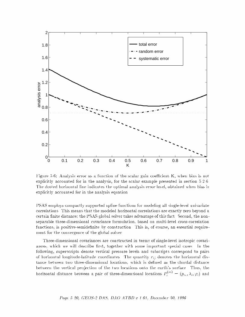
total error
random error
systematic error
0 0.1 0.2 0.3 0.4 0.5 0.6 0.7 0.8 0.9 10
0.2
0.4
0.6
0.8
1
1.2
1.4
1.6
1.8
2
K
anal
ysis
err
or
Figure 5.6: Analysis error as a function of the scalar gain coe�cient K, when bias is not
explicitly accounted for in the analysis, for the scalar example presented in section 5.2.6.
The dotted horizontal line indicates the optimal analysis error level, obtained when bias is
explicitly accounted for in the analysis equation.
PSAS employs compactly supported spline functions for modeling all single-level univariate
correlations. This means that the modeled horizontal correlations are exactly zero beyond a
certain �nite distance; the PSAS global solver takes advantage of this fact. Second, the non-
separable three-dimensional covariance formulation, based on multi-level cross-correlation
functions, is positive-semide�nite by construction. This is, of course, an essential require-
ment for the convergence of the global solver.
Three-dimensional covariances are constructed in terms of single-level isotropic covari-
ances, which we will describe �rst, together with some important special cases. In the
following, superscripts denote vertical pressure levels and subscripts correspond to pairs
of horizontal longitude-latitude coordinates. The quantity rij denotes the horizontal dis-
tance between two three-dimensional locations, which is de�ned as the chordal distance
between the vertical projection of the two locations onto the earth's surface. Thus, the
horizontal distance between a pair of three-dimensional locations P(m)i = (pm; �i; 'i) and
Page 5.20, GEOS-2 DAS, DAO ATBD v 1.01, December 30, 1996

P(n)j = (pn; �j; 'j) is given by
rij = [(pi � pj) � (pi � pj)]12 = a [2(1� qi � qj)]
12 ; (5.53)
where a is the earth's radius and
pj = aqj = a [cos'j cos�j; cos'j sin�j ; sin'j ] : (5.54)
5.2.7.1.1.1 Single-level univariate isotropic covariances
The general single-level univariate isotropic covariance model is of the form
[Cov](m)ij = �
(m)i �
(m)j �(m)(rij); (5.55)
where �(m)(r) is a correlation function and �(m) > 0.
Although PSAS does not contain any restrictions on the type of correlation models it
can handle, only a few families of single-level correlation models are actually employed. For
errors which are assumed horizontally uncorrelated,
�(m)(r) = �(r) (5.56)
where
�(r) =
(1 if r = 0
0 otherwise(5.57)
Horizontally correlated errors may be modeled using the powerlaw function, given by
�(m)(r) = �p(r;L(m)) =
"1 +
1
2
�r
L(m)
�2#�1: (5.58)
Alternatively, the compactly supported spline function (Gaspari and Cohn, section 4.3) can
be used:
�(m)(r) = �c(r;L(m)) (5.59)
where
�c(r;L(m)) =
8><>:�1
4
�rc
�5+ 1
2
�rc
�4+ 5
8
�rc
�3 � 53
�rc
�2+ 1; if 0 � r � c;
112
�rc
�5 � 12
�rc
�4+ 5
8
�rc
�3+ 5
3
�rc
�2 � 5�rc
�+ 4� 2
3
�rc
��1; if c � r � 2c;
0 otherwise
(5.60)
with
c = L(m)
r10
3: (5.61)
Page 5.21, GEOS-2 DAS, DAO ATBD v 1.01, December 30, 1996
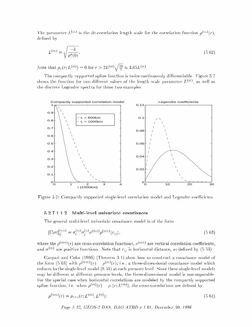
The parameter L(m) is the de-correlation length scale for the correlation function �(m)(r),
de�ned by
L(m) =
s�1�00c (0)
: (5.62)
Note that �c(r;L(m)) = 0 for r > 2L(m)
q103� 3:65L(m).
The compactly supported spline function is twice continuously di�erentiable. Figure 5.7
shows the function for two di�erent values of the length scale parameter L(m), as well as
the discrete Legendre spectra for these two examples.
L = 500km
L = 1000km
0 1 2 3 40
0.1
0.2
0.3
0.4
0.5
0.6
0.7
0.8
0.9
1
r [1000km]
Compactly supported correlation model
0 10 20 300
0.02
0.04
0.06
0.08
0.1
0.12Legendre coefficients
Figure 5.7: Compactly supported single-level correlation model and Legendre coe�cients.
5.2.7.1.1.2 Multi-level univariate covariances
The general multi-level univariate covariance model is of the form
[Cov](mn)ij = �
(m)i �
(n)j �(mn)�(mn)(rij); (5.63)
where the �(mn)(r) are cross-correlation functions, �(mn) are vertical correlation coe�cients,
and �(m) are positive functions. Note that rij is horizontal distance, as de�ned by (5.53).
Gaspari and Cohn (1996) (Theorem 3.1) show how to construct a covariance model of
the form (5.63) with �(mm)(r) = �(m)(r); i.e., a three-dimensional covariance model which
reduces to the single-level model (5.55) at each pressure level. Since these single-level models
may be di�erent at di�erent pressure levels, the three-dimensional model is non-separable.
For the special case when horizontal correlations are modeled by the compactly supported
spline function, i.e. when �(m)(r) = �c(r;L(m)), the cross-correlations are de�ned by
�(mn)(r) = �c�c(r;L(m); L(n)); (5.64)
Page 5.22, GEOS-2 DAS, DAO ATBD v 1.01, December 30, 1996

the formula for this family of functions is rather cumbersome and will not be included here.
Figure 5.8 shows an example of a compactly supported spline cross-correlation function.
The covariance model 5.63 is positive-semide�nite by construction, provided the vertical
correlation matrix [�](mn) is positive-semide�nite.
When all single-level correlation functions are identical, i.e., �(m)(r) = �(r) for all m,
(5.63) reduces to the separable model
[Cov](mn)ij = �
(m)i �
(n)j �(mn)�(rij): (5.65)
single−level correlation (L = 500km)
single−level correlation (L = 1000km)
cross correlation
0 0.5 1 1.5 2 2.5 3 3.5 40
0.1
0.2
0.3
0.4
0.5
0.6
0.7
0.8
0.9
1
r [1000km]
Compactly supported spline cross−correlation model
Figure 5.8: Compactly supported spline cross-correlation function.
5.2.7.1.2 Tuning methodology. The actual multivariate error covariance formula-
tions employed by PSAS can all be expressed in terms of the general univariate model
presented in the previous section. In general, assumptions about forecast and observation
errors (which will be described below, in sections 5.2.7.2 and 5.2.7.3) lead to parameterized
covariance models of the form
Pfk � P
fk (�
f); Rk � Rk(�o); (5.66)
Page 5.23, GEOS-2 DAS, DAO ATBD v 1.01, December 30, 1996

where Pfk ; Rk are the forecast and observation error covariances at time tk, respectively.
The �f ; �o are covariance parameters which must be estimated from data; these may in-
clude observation error standard deviations, horizontal de-correlation length scales, vertical
correlation coe�cients, etc.
Observational information about the covariance parameters �f ; �o is contained in the
observed-minus-forecast residuals (O-F's)
vk � wok � hk(wfk): (5.67)
Here wok is any vector of observations and wfk is the forecast valid at time tk . The observation
operator hk maps model state variables to the observables; if the state variables are observed
directly then hk is just an interpolation operator, but in case of radiance data, for example,
the observation operator involves a radiative transfer model. In general one can de�ne the
linearized observation operator Hk:
Hk �@hk
@w
����w=w
f
k
: (5.68)
The forecast as well as the observations themselves contain errors, and therefore the
residual (5.67) depends on both forecast errors and observation errors. In fact, it is easy to
show that the covariance of the O-F's equals the sum of the forecast and observation error
covariances:
Sk �D(vk � hvki)(vk � hvki)T
E(5.69)
� Rk +HkPfkH
Tk ; (5.70)
under the assumption that forecast and observation errors are statistically independent. In
case of direct observations of state variables, the matrix HkPfkH
Tk is just the evaluation of
the forecast error covariance model at the observation locations.
The residual covariance equation (5.69) provides the basis for tuning forecast and ob-
servation error statistics for given covariance formulations. Substitution of the covariance
models (5.66) yields
Sk � Sk(�) = Sk(�f ; �o): (5.71)
Estimates of � can be obtained by �nding the best �t of the covariance model xk(�) to a
sequence of residuals
fvkg � fvk; k = 1; : : : ; Kg: (5.72)
In doing so we assume that the mean hvki is zero; in practice the (time) mean of fvkg is
removed prior to covariance tuning.
The criterion of �t is based on the maximum-likelihood principle, in which the likelihood
function of the data is maximized as a function of the unknown parameters �. We assume
Page 5.24, GEOS-2 DAS, DAO ATBD v 1.01, December 30, 1996

that the time-series of O-F's is white and Gaussian, with mean zero and covariance at time
tk given by Sk(�) for some �. Then
p(fvkg;�) =KYk=1
p(vk;�) /KYk=1
(detSk(�))�
12 exp
��1
2vTk S
�1k (�)vk
�: (5.73)
The maximum-likelihood estimate �̂ is obtained by maximizing (5.73), or, equivalently, by
minimizing the log-likelihood function
f(�) =KXk=1
hlog detSk(�) + vTk S
�1k (�)vk
i: (5.74)
In case the covariance model (5.71) is stationary, i.e.
Sk(�) = S(�); (5.75)
the log-likelihood function simpli�es to
f(�) = K �hlog detS(�) + tr(S�1(�) bS)i : (5.76)
Here bS is the sample covariance of the data de�ned by
bS =1
K
KXk=1
vkvTk ; (5.77)
where, if necessary, the mean of the time series fvkg has been removed. For a stationary
observing system, such as a rawinsonde observing network, (5.76) is easier to evaluate than
(5.74).
The tuning method just described is quite general, and can be used to tune all kinds of
covariance parameters. To illustrate the method we describe its application to the tuning of
the forecast height error horizontal correlation length scales based on single-level rawinsonde
height observed-minus-forecast residuals. At a �xed pressure level, the covariance of these
residuals is given by
Sij = �o�(rij) + �f�c(rij;L); (5.78)
where �o is the rawinsonde height observation error standard deviation, �f is the forecast
height error standard deviation, and L is the length scale parameter for the forecast height
error horizontal correlations. These parameters can be estimated from, say, a month of
data, by computing the sample covariance bS of the data de�ned at the station locations,
and then minimizing (5.76) as a function of the three parameters � = (�o; �f ; L).
As an example we take 500hPa data from 80 North-American rawinsonde stations for the
month of February, 1995. For this case one obtains the estimates �o = 9:2m; �f = 12:4m;
and L = 617� 103m. Individual elements of bS are plotted in �gure 5.9 together with the
Page 5.25, GEOS-2 DAS, DAO ATBD v 1.01, December 30, 1996

0 0.5 1 1.5 2 2.5 3 3.5 4
x 106
−50
0
50
100
150
200
250
300
350500hPa North−American rawinsonde height O−F covariances
Figure 5.9: Sample and tuned model covariances for 500hPa North-American rawinsonde
height observed-minus-forecast residuals.
model �t. The scatter in the sample covariances is due to sampling error as well as to
the fact that actual errors are neither isotropic nor stationary. The model �t is plotted as
well. At �rst glance it may seem that the model underestimates the covariances, however
upon closer inspection this is primarily due to the large scatter of the sample covariances
beyond 103m. The maximum-likelihood criterion apparently rejects this scatter as being
statistically insigni�cant.
5.2.7.2 Speci�cation of forecast error statistics
This section describes the multivariate, three-dimensional formulation of the forecast error
covariance model.
Page 5.26, GEOS-2 DAS, DAO ATBD v 1.01, December 30, 1996

5.2.7.2.1 Forecast height errors. The forecast height error covariance model is of the
form
[Cov](mn)ij = �
(m)i �
(n)j �(mn)�c�c(rij;L
(m); L(n)): (5.79)
The main features of this model are:
1. the height error variances are three-dimensional, spatially variable �elds which are
updated on-line;
2. the correlation model has compact support;
3. correlations are horizontally isotropic (correlations at �xed pressure levels depend on
distance only);
4. the model is non-separable (horizontal de-correlation length scales may vary with
pressure).
The length scale parameters L(m) in the model (5.79) are estimated from single-level
rawinsonde height O-F's. The vertical correlation coe�cients �(mn) are estimated from
multi-level rawinsonde height O-F's. The forecast height error standard deviations � are
estimated from global time series of TOVS height retrievals, as follows.
5.2.7.2.1.1 Speci�cation of height error variances
The height forecast error variances are again estimated from observed-minus-forecast
residuals (O-F's). The maximum-likelihood methodology described earlier provides spa-
tially averaged estimates of the forecast variances valid at the tuning region, usually North
America. In order to account for the regional variability of the forecast error variances, we
use global residual time series instead.
We start by binning the residuals on a 4� by 5� latitude-longitude grid, computing
mean and standard deviations for each grid-box. This calculation is performed separately
for radiosonde height observations (RAOB) and NESDIS TOVS A/B retrievals (TOVS). For
those grid-boxes with more than 10 radiosonde observations in a given month, we assume
��f jhj
�2��sRAOBj
�2���RAOB
�2(5.80)
where sRAOBj is the radiosonde O-F standard deviation for grid-box j at a given level (we
have omitted the vertical level index (m) for notational convenience), and �RAOB is the
radiosonde observation error standard deviation, tuned over North America and assumed
constant over the globe. We have also assumed statistical independence of forecast and
observation errors. Because radiosonde coverage is mostly restricted to the northern hemi-
sphere land areas, the only hope for obtaining a global estimate of forecast error variances
is to use satellite observations. The TOVS O-F variance can be written
�sTOV Sj
�2=��f jhj
�2+��TOVSu
�2+��TOV Sc
�2� 2xj (5.81)
Page 5.27, GEOS-2 DAS, DAO ATBD v 1.01, December 30, 1996

Figure 5.10: Square-root of zonal average of forecast height error variances estimated
from radiosondes (eq. 5.80, open circles), modi�ed TOVS height innovation variances
(�sTOV Sj
�2 � ��TOVSu
�2, closed circles), and forecast height error variances estimated from
TOVS (eq. 5.82, solid line). Monthly means for December 1991, at 250 hPa. Units: meters
where �TOVSu ; �TOVSc are the standard deviations of the spatially uncorrelated and corre-
lated components of the retrieval error, respectively (see section 5.2.7.3.2 below), and xjis the cross-covariance between the retrieval and forecast errors at locations i and j. Da
Silva et al. (1996) present a method for estimating each term on the RHS of (5.81); however
these estimates are only valid regionally. Terms such as �TOV Sc and xj are likely to vary
spatially as much as the forecast error standard deviation itself; the uncorrelated portion
of the retrieval error, �TOVSu , has been veri�ed to have a modest variation over the globe.
In view of this, we adopt the following parameterization for �f jhj in terms of TOVS O-F's:
��f jhj
�2� �2('j)
��sTOV Sj
�2���TOVSu
�2�+ d (5.82)
where � is an empirical function of latitude de�ned by
�2('j; a; b; c) = a exph� ('j=b)
2i+ c; (5.83)
Page 5.28, GEOS-2 DAS, DAO ATBD v 1.01, December 30, 1996

and a; b; c; d are constants. These four parameters are determined separately for each vertical
level by means of a non-linear least-square �t of the model (5.80) to co-located radiosonde
estimates of��f jhj
�2, obtained from (5.80). Once model parameters (a; b; c; d) are deter-
mined for each level (levels above 20 hPa use the same value of the parameters at 20 hPa),
forecast error variances determined from radiosondes and TOVS retrievals are merged to-
gether and smoothed with a simple successive correction method. An example of zonally
averaged forecast error standard deviations obtained by this procedure is shown in Fig. 5.10.
As discussed in subsection (5.2.6), unless forecast bias is explicitly accounted for, the
forecast error variances must be in ated based on an estimate of this bias. A zonally
symmetric estimate of the time-averaged forecast error can be obtained by �tting the model
bf('j ; a; b; c; d) = a exp
"��'j � d
b
�2#+ c (5.84)
to gridded, zonal-time mean radiosonde O-F's, for each level. An example of such a �tted
forecast bias model is shown in Fig. 5.11. The �nal three-dimensional gridded �eld of
forecast error variances used by PSAS is:
��f jhj
�2=��f jhj
�2+�bf('j)
�2(5.85)
Running monthly means of O-F standard deviations are re-computed on a daily basis,
model parameters re-tuned, and �f jhj updated. Although model parameters are robust
and do not change much on a daily basis, this adaptive system is capable of capturing the
seasonal cycle in the forecast error variances and to automatically keep up with modi�cations
made in the data assimilation system.
5.2.7.2.2 Forecast wind errors. The multivariate height-wind covariance formulation
is based on the following model for wind errors. Denoting the wind error �eld by u; v, it is
assumed that
"u
v
#=
"uhvh
#+
"udvd
#(5.86)
where uh; vh is the height-coupled wind error component (correlated with height errors) and
ud; vd is the height-decoupled wind error component (statistically independent from height
errors). The two wind error components are assumed mutually independent, and a separate
model exists for each.
5.2.7.2.2.1 Height-coupled wind error component
The height-coupled wind error component is modeled by assuming a linear relationship
of the form
"uhvh
#=
g
2
"a11('; p) a12('; p)
a21('; p) a22('; p)
# "@h@x@h@y
#(5.87)
Page 5.29, GEOS-2 DAS, DAO ATBD v 1.01, December 30, 1996

Figure 5.11: Monthly means for December 1991 of radiosonde height innovations at 50 hPa
(open circles), and zonally symmetric �t (solid line). Units: meters
The coe�cients aij are parameterized by
a11 = a22 =�c
(m)0 �(';p)
�2(';p)+sin2(')(5.88)
�a12 = a21 = sin(')
�2(';p)+sin2(')(5.89)
where
�2('; p) = c(m)1 exp
24�
'
c(m)2
!235 : (5.90)
Note that �('; p) for p = pm �xed attains a maximum value of c(m)1 at the equator, and
decays exponentially away from the equator. When � ! 0, the model (5.87) reduces to
the geostrophic balance relation. The values of the model parameters c(m)0 ; c
(m)1 ; c
(m)2 are
obtained by regression to a time-series of 48h-24h forecast residuals.
Page 5.30, GEOS-2 DAS, DAO ATBD v 1.01, December 30, 1996

Given the height error covariance (5.79), the model (5.87) completely determines the
multivariate height-coupled wind error covariance.
5.2.7.2.2.2 Height-decoupled wind error component
The height-decoupled wind error component is modeled in terms of a stream function
and a velocity potential � by
"udvd
#=
"�@ @y +
@�@x
@ @x
+ @�@y
#(5.91)
The stream function and velocity potential are assumed mutually independent, and the
covariance model for each is of the form
[Cov](mn)ij = �(m)�(n)�(mn)�c�c(rij;L
(m); L(n)): (5.92)
The model parameters �(m); L(m) for both stream function and velocity potential are esti-
mated from single-level rawinsonde height and wind O-F's. The vertical correlation coe�-
cients (�)(mn) for both stream function and velocity potential are estimated from multi-level
rawinsonde height and wind O-F's.
5.2.7.2.3 Forecast moisture errors. The forecast moisture error covariance model is
of the form
[Cov](mn)ij = (�(m))2�(m� n)�c(rij ;L
(m)): (5.93)
The main features of this model are:
1. the variances are constant at each pressure level;
2. correlations have compact support;
3. correlations are horizontally isotropic, i.e. at �xed pressure levels;
4. horizontal de-correlation length scales vary in the vertical direction.
The model parameters �(m); L(m) are estimated from rawinsonde mixing ratio observations.
5.2.7.3 Speci�cation of observation error statistics
5.2.7.3.1 Rawinsonde errors. Rawinsonde errors are assumed to be vertically corre-
lated but uncorrelated in the horizontal direction. Height, wind, and moisture observation
errors are assumed independent of each other. Each of the univariate rawinsonde observa-
tion error covariance models are of the form
[Cov](mn)ij = �(m)�(n)�(mn)�(rij): (5.94)
Page 5.31, GEOS-2 DAS, DAO ATBD v 1.01, December 30, 1996

Height error observation error standard deviations are estimated from single-level rawin-
sonde height O-F's; the vertical correlation coe�cients are estimated from multi-level rawin-
sonde height O-F's. Similarly, the error statistics for mixing ratio observations are estimated
from rawinsonde mixing ratio O-F's. Wind observation error statistics are estimated from
multivariate (height and wind) O-F's.
5.2.7.3.2 TOVS height retrieval errors. TOVS height retrieval errors are assumed
to consist of two components, one of which is horizontally uncorrelated. The covariance
model is of the form
[Cov](mn)ij = �(m)
u �(n)u �(mn)u �(rij) + �(m)c �(n)c �(mn)c �c(rij ;L
(m)): (5.95)
The main features of this model are:
1. height retrieval errors contain a component which is horizontally uncorrelated;
2. the retrieval error standard deviations are constant at each pressure level;
3. the correlation model has compact support;
4. correlations are horizontally isotropic: correlations at �xed pressure levels depend on
distance only;
5. horizontal de-correlation length scales vary in the vertical direction.
The parameters �(m)u are estimated from single-level retrieval O-F's. The vertical cor-
relation coe�cients �(mn)u are estimated from multi-level retrieval O-F's. The parameters
�(m)c ; L(m) are estimated from single-level co-located retrieval-minus-rawinsonde observa-
tions (O-O's). The vertical correlation coe�cients �(mn)c are estimated from multi-level
co-located retrieval-minus-rawinsonde O-O's.
Details of this procedure are described in da Silva et al. (1996), where it is also shown how
the tuning methodology can be applied to the estimation of the cross-covariance between
forecast and observation errors.
Page 5.32, GEOS-2 DAS, DAO ATBD v 1.01, December 30, 1996

5.3 The GEOS-2 General Circulation Model
5.3.1 Introduction and Model Lineage
The Goddard Earth Observing System-2 (GEOS-2) General Circulation Model (GCM) is
an incremental development of the GEOS-1 GCM. The develop paths have been chosen
based on the major Earth-science priorities discussed in Chapter 2.0 as well as the ex-
perience gained in both model and data assimilation applications. Many of the changes
made in GEOS-2 are in preparation for extended capabilities in GEOS-3. Major GEOS-3
developments will focus on the implementation of an interactive land-surface model and
prognostic cloud water parameterization. These improvements are driven not only by the
need to improve cloud and hydrological processes, but the need to monitor and assimilate
new data types.
Unlike the development of PSAS and the associated error statistics, much of the GCM
development is linked with other modeling e�orts within Goddard. While this potentially
saves resources by leveraging o� of existing expertise, it is not without cost. Often seem-
ingly appropriate algorithms are not easily integrated into the GEOS GCM. This can occur
because the native model in which the algorithm was developed has its own set of compen-
sating errors, for which the algorithm has been explicitly or implicitly tuned. Sometimes
the software engineering of candidate algorithms is so poor that it is easier to start an in-
dependent development rather than implement foreign code. In addition, the management
structure of GSFC is not conducive for entraining non-DAO scientists into a product- and
time- driven development. It is one of the management goals of the DAO to develop a
model infrastructure that facilitates inside and outside collaboration. The GEOS model
and analysis system must become a resource that attracts visiting scientists and outside
experts, if the GEOS DAS is to achieve its full potential.
The GEOS-2 GCM was developed by the Data Assimilation O�ce (DAO) at the God-
dard Laboratory for Atmospheres (GLA), in collaboration with the Climate and Radiation
Branch, for use in the system being developed to analyze EOS data. Based on extensive
analysis and evaluation of the GEOS-1 system (see Takacs and Suarez (1996), Molod et al.
(1996), Schubert et al. (1995), Schubert and Rood (1995)), the GEOS-2 GCM addresses
some of the fundamental limitations of GEOS-1. The GEOS-2 GCM also provides the next
benchmark and infrastructure base in the DAO's e�ort to develop the GEOS-3 system for
the EOS observing period. Development advances of the GEOS-2 GCM relative to the
GEOS-1 GCM will be speci�cally highlighted at the beginning of the appropriate sections.
As noted, the immediate predecessor of the GEOS-2 GCM was the GEOS-1 GCM which
was used to produce a multi-year global atmospheric data set for climate research (Schu-
bert et al., 1993). The GEOS-1 GCM was also used to produce multiple 10-year climate
simulations as part of the DAO's participation in the Atmospheric Model Intercomparison
Project (AMIP) sponsored by the Program for Climate Model Diagnostics and Intercom-
parison (PCMDI) (see Gates, 1992). A stratospheric version of the GEOS DAS (Version
1.2) has been used operationally to provide scienti�c ight guidance during NASA's partic-
ipation in the Measurements for Assessing the E�ects of Stratospheric Aircraft (MAESA)
and other �eld experiments.
The earliest predecessor of the GEOS-1 GCM was developed in 1989 based on the
Page 5.33, GEOS-2 DAS, DAO ATBD v 1.01, December 30, 1996

\plug- compatible" concepts outlined in Kalnay et al. (1989), and subsequently improved
in 1991 (Fox- Rabinovitz, et al., 1991, Helfand et al., 1991). The plug-compatibility of the
physical parameterizations together with the plug-compatible \Dynamical Core" introduced
by Suarez and Takacs (1995) facilitate the development and testing of new algorithms.
Together the DAO and the Climate and Radiation Branch at GLA have produced a library
of physical parameterizations and dynamical algorithms which can be utilized for various
GCM applications.
Relevant Model Documentation
Descriptions of aspects of the the GEOS Data Assimilation System (DAS) may be found
in Schubert et al. (1993), Pfaendtner et al. (1995) and Bloom et al. (1996). The GEOS-1
GCM is documented in Takacs et al. (1994), and for completeness much of the GEOS-1
documentation is included here to provide a self-contained report of the GEOS-2 GCM.
A comprehensive documentation of the Aries/GEOS Dynamical Core incorporating the
horizontal and vertical discretization and �nite-di�erence schemes used is given in Suarez
and Takacs (1995). The Relaxed Arakawa-Schubert cumulus convective parameterization
and the re-evaporation of falling rain are based upon the works of Moorthi and Suarez
(1992) and Sud and Molod (1988). The longwave radiative processes are described by Chou
and Suarez (1994) and the shortwave by Chou (1990) and Chou (1992). The turbulence
parameterization is based on the Level 2.5 second order closure scheme of Helfand and
Labraga (1988), and the surface layer parameterization in described in Helfand and Schubert
(1995). The gravity wave drag parameterization is based on Zhou et al. (1996).
5.3.2 Atmospheric Dynamics
The momentum equations used in the GEOS-2 GCM are written in the \vector invariant"
form, as in Sadourney (1975) and Arakawa and Lamb (1981), to facilitate the derivation
of the energy and potential enstrophy conserving di�erencing scheme. The thermodynamic
(potential temperature) and moisture (speci�c humidity) equations are written in ux form
to facilitate potential temperature and moisture conservation. A complete description of
the �nite-di�erence scheme used can be found in Suarez and Takacs (1995).
The GEOS GCM uses a � coordinate de�ned by
� =p� pT
�; (5.96)
where p is the pressure, � � ps � pT , ps is the surface pressure, and pT is a constant
prescribed pressure at the top of the model atmosphere. With pT = 0 this coordinate
reduces to the conventional � coordinate proposed by Phillips (1957).
With this vertical coordinate, the continuity equation becomes
@�
@t= �r� � (�v)�
@(� _�)
@�; (5.97)
where v is the horizontal velocity vector. Integrating (5.97) and assuming _� = 0 at p = ps
Page 5.34, GEOS-2 DAS, DAO ATBD v 1.01, December 30, 1996

and p = pT , we obtain the forms used in the model:
@�
@t= �
Z 1
0r� � (�v) d� (5.98)
and
(� _�) = ��@�@t
�Z �
0r� � (�v) d�: (5.99)
The equation of state for an ideal gas is � = RT=p, where � is the speci�c density, T
is the temperature, and R is the gas constant. The following alternative forms will be used
below
� = R�P
p= cp�
@P
@p=cp�
�
�@P
@�
��
=cp�
�
�@P
@�
��
; (5.100)
where � � T=P is the potential temperature, P � (p=p0)�, � = R=cp, cp is the speci�c heat
at constant pressure, and p0 is a reference pressure. In obtaining the forms in (5.100) we
have used @P@p
= �Ppand the relation
�dP
d�
��
=�
�
�dP
d�
��
: (5.101)
For the time being virtual e�ects are neglected.
The hydrostatic equation is@�
@p= ��;
where � is the geopotential. Using (5.100) and (5.101), this can be written:
@�
@�= ��� = �cp�
�
�
�dP
d�
��
= �cp��dP
d�
��
: (5.102)
From (5.102) we obtain
@�
@P= �cp�; (5.103)
which, following Arakawa and Suarez (1983), is the form used in the model.
The momentum equation is written in \vector-invariant" form, as in Sadourney (1975)
and Arakawa and Lamb (1981), to facilitate the derivation of an energy- and enstrophy-
conserving di�erencing scheme:
@v
@t= �(f + �)k� v � _�
@v
@��r�(�+K)� cp�r�P � g
�
@T@�
; (5.104)
= �� k� (�v)� _�@v
@��r�(� +K)� cp�
�dP
d�
��
r� � g
�
@T@�
; (5.105)
Page 5.35, GEOS-2 DAS, DAO ATBD v 1.01, December 30, 1996
where
� =(f + �)
�
is an \external" potential vorticity, f is the Coriolis parameter, k is the unit vector in the
vertical,
� � r� � v
is the vertical component of the vorticity along � surfaces,
K � 1
2(v � v)
is the kinetic energy per unit mass, g is the acceleration of gravity, and T is the horizontal
frictional stress.
The thermodynamic equation is written in ux form to facilitate the derivation of a
�-conserving di�erencing scheme:
@(��)
@t= �r� � (�v�)�
@(� _��)
@�+�QcpP
; (5.106)
where Q is the diabatic heating per unit mass.
In addition to the equations of motion, the Aries/GEOS Dynamical Core computes
tendencies for an arbitrary number of atmospheric contituents, such as water vapor and
ozone. These are also written in ux form:
@(�q(k))
@t= �r� � (�vq(k))�
@(� _�q(k))
@�+ �S(k); (5.107)
where q(k) is the speci�c mass of the kth constituent, and S(k) is its source per unit mass
of air.
5.3.2.1 Horizontal and Vertical Discretization
The GEOS-2 GCM is constructed in the horizontal using the staggered Arakawa C-grid
(see Figure 5.12) and employs Version 2 of the Aries/GEOS Dynamical Core for the �nite-
di�erencing algorithm. Important di�erences relative to GEOS-1 include
� fourth order horizontal di�erences instead of second order
� raising the model top to 0.01 hPa
� increasing the vertical resolution to 70 levels
The use of fourth order di�erencing substantially improves the phase propagation of
synoptic scale waves. The raising of the model lid is directed at improving stratospheric
descent over the winter pole and addressing the stratospheric cold pole problem. Increasing
the number of level is directed at improving the representation of the planetary boundary
layer, the troposphere at the altitude of the sub-tropical jet stream, and the stratosphere.
Page 5.36, GEOS-2 DAS, DAO ATBD v 1.01, December 30, 1996

i
j�i;j
z }| {�x
8>>>>>>>>>>>>>>>>>>>><>>>>>>>>>>>>>>>>>>>>:
�yui+ 1
2;jui� 1
2;j
vi;j� 12
vi;j+ 12
�i� 12;j� 1
2�i+ 1
2;j� 1
2
�i� 12;j+ 1
2�i+ 1
2;j+ 1
2
Figure 5.12: Stencil showing the position and indexing of the prognostic �elds u, v, �, and
�.
The Aries/GEOS Dynamical Core is a plug-compatible dynamics module which is used
at both the DAO in the GEOS GCM as well as at the Climate and Radiation Branch in
the Aries GCM. The Aries GCM has been extensively used in many climate and coupled
ocean/atmosphere simulations (eg. Schubert et al. 1993, Higgins and Schubert, 1993).
Version 2 of the Aries/GEOS Dynamical Core is a fourth-order version of the Sadourny en-
ergy and potential enstrophy conserving scheme described by Burridge and Haseler (1977),
and is fully derived in Suarez and Takacs (1995). This scheme conserves total energy and
potential enstrophy for the non-divergent component of the ow in the shallow water equa-
tions. It is fourth-order in the sense that it reduces to the fourth-order Arakawa (1966)
Jacobian for non-divergent ow. It thus provides fourth-order accuracy for the advection
of a second-order vorticity by the non-divergent part of the ow. Horizontal advection of
potential temperature and moisture is performed using the fourth-order scheme in use in
the UCLA GCM (Arakawa, personal communication). It also is fourth-order only in the
advection by the non-divergent part of the ow.
The Aries/GEOS Dynamical Core uses a Lorenz or unstaggered vertical grid in gen-
eralized sigma coordinates (see Figure 5.13). The vertical di�erencing scheme is that of
Arakawa and Suarez (1983) which ensures that:
� The pressure gradient force generates no circulation of vertically in-
tegrated momentum along a contour of surface topography� The �nite-di�erence analogues of the energy-conversion term have
the same form in the kinetic energy and thermodynamic equations� The global mass integral of the potential temperature is conserved
under adiabatic processes
Page 5.37, GEOS-2 DAS, DAO ATBD v 1.01, December 30, 1996

� The hydrostatic equation for the lowest thickness has a local form
� The hydrostatic equation is exact for vertically isentropic atmo-
spheres� The pressure-gradient force is exact for three-dimensionally isen-
tropic atmospheres
`� 1
`e
`u v � � P� q !
� _�
u v � � P� q !
Figure 5.13: Vertical placement and index notation for sigma levels in the GEOS-2 GCM
The standard, or \production", resolution of the GEOS-2 GCM is a global 2� x 2:5� latitude-
longitude grid in the horizontal, together with 70 sigma levels in the vertical. The vertical
distribution of the sigma levels (shown in Table 5.2) is chosen to provide enhanced resolu-
tion in the planetary boundary layer and at the tropospheric jet level, as well as providing
a well resolved stratosphere. The model top pressure used in this con�guration is set at
0.01 hPa. Figure 5.14 shows the distribution of levels based on 1000 hPa surface pressure.
The logarithm of pressure and �pressure are used to show detail in the upper levels. There
are 8 levels within the lowest 100 hPa, and approximately 40 levels below 10 hPa (note,
GEOS-1 had 2 and 20 levels, respectively). Figure 5.15 shows the distribution of the lowest
10 levels in detail.
5.3.2.2 Time Integration Scheme
The GEOS GCM has the ability to use the Matsuno time integration scheme or the Leapfrog
time integration scheme together with an Asselin (1972) time �lter. The GEOS-1 GCM
multi-year simulations cited in Takacs and Suarez (1996) and Molod et al. (1996) used the
Leapfrog time scheme together with the Asselin averaging parameter equal to 0.05. The
GEOS-1 DAS multi-year Re-analysis used the Matsuno time scheme. The GEOS GCM
employs a unique method for incorporating adjustments due to diabatic processes (ie, moist
convection, radiation and turbulence) and the analysis increments during an assimilation.
At every model time step, all prognostic �elds are updated due to both dynamical and
Page 5.38, GEOS-2 DAS, DAO ATBD v 1.01, December 30, 1996

Figure 5.14: Vertical distribution used in the 70-level GEOS-2 GCM.
Page 5.39, GEOS-2 DAS, DAO ATBD v 1.01, December 30, 1996

Figure 5.15: Vertical distribution used in the lowest 10 levels of the GEOS-2 GCM.
Page 5.40, GEOS-2 DAS, DAO ATBD v 1.01, December 30, 1996

Table 5.2: GEOS-2 Sigma Level Distribution
Level Sigma � Sigma Level Sigma � Sigma Level Sigma � Sigma
1 .000003 .000006 25 .005699 .001162 49 .316175 .039790
2 .000010 .000008 26 .006982 .001402 50 .357260 .042380
3 .000018 .000009 27 .008526 .001687 51 .400740 .044580
4 .000028 .000011 28 .010381 .002022 52 .446215 .046370
5 .000041 .000014 29 .012600 .002416 53 .493218 .047635
6 .000057 .000018 30 .015247 .002878 54 .541227 .048384
7 .000077 .000023 31 .018394 .003416 55 .589634 .048431
8 .000103 .000029 32 .022123 .004042 56 .637724 .047750
9 .000136 .000037 33 .026527 .004767 57 .684748 .046297
10 .000179 .000047 34 .031710 .005600 58 .729920 .044048
11 .000232 .000060 35 .037793 .006566 59 .772457 .041026
12 .000300 .000076 36 .044898 .007644 60 .811635 .037330
13 .000386 .000095 37 .053147 .008854 61 .846935 .033270
14 .000494 .000120 38 .062692 .010237 62 .878157 .029174
15 .000628 .000149 39 .073724 .011825 63 .905322 .025156
16 .000795 .000185 40 .086444 .013616 64 .928565 .021330
17 .001003 .000230 41 .101065 .015626 65 .948115 .017770
18 .001261 .000285 42 .117817 .017877 66 .964250 .014500
19 .001579 .000352 43 .136943 .020375 67 .977200 .011400
20 .001971 .000433 44 .158715 .023170 68 .987150 .008500
21 .002453 .000531 45 .183425 .026250 69 .994248 .005695
22 .003043 .000649 46 .211400 .029700 70 .998548 .002905
23 .003763 .000791 47 .242900 .033300
24 .004638 .000960 48 .277915 .036730
sub-grid scale diabatic processes, shown schematically using the Leapfrog time scheme for
an arbitrary prognostic �eld q as:
qn+1 = qn�1 + 2�t
�@q
@t
n�total
(5.108)
where
�@q
@t
n�total
=
�@q
@t
n�Dynamics
+
@q
@t
n�1!Shapiro F ilter
+
�@q
@t
�Moist Processes
+
�@q
@t
�Turbulence
+
�@q
@t
�GravityWaveDrag
Page 5.41, GEOS-2 DAS, DAO ATBD v 1.01, December 30, 1996

+
�@q
@t
�Longwave Radiation
+S0
R2a
� cos�z�@q
@t
�Shortwave Radiation
+
�@q
@t
�Analysis Increment
(5.109)
with S0 de�ned as the solar contant, Ra as the earth-sun distance in Astronomical Units,
and cos�z as the cosine of the zenith angle. The Dynamics and Shapiro Filter time ten-
dencies are updated every model time step using the time index indicated in (5.109). The
diabatic time tendencies are updated at a time step appropriate to the physical parameteri-
zations using the current time index, and are held constant between Physics calls. The time
tendency for Moist Convection is updated every 10 minutes, and for Turbulence every 30
minutes. The time tendency for Longwave Radiation is updated every 3 hours. Shortwave
Radiation is updated once every three hours assuming a normalized incident solar radiation,
and adjusted at every model time step by the true incident radiation. During GEOS-2 DAS
assimilations, the Analysis Increment is updated every synoptic time period, or 6 hours.
By gradually incorporating the diabatic adjustments during the model integration, shocks
and dynamical imbalances are greatly reduced (cf. Bloom, et al. 1996).
5.3.2.3 Coordinate Rotation
In GEOS-2 the capability to perform a coordinate rotation of the �nite di�erence grid has
added. This was implemented to address polar noise problems, especially in the strato-
sphere. In addition, the coordinate rotation is at the basis for adaptive resolution capabili-
ties to provide the infrastructure for possible regional applications.
As previously mentioned, the Eulerian grid-point dynamics module used in the GEOS
GCM is the Aries/GEOS Dynamical Core (Suarez and Takacs, 1995). This module allows
the spherical coordinate system used for the computations to be displaced relative to the
geographical latitude-longitude coordinates. The relation between the two coordinate sys-
tems is fully determined by specifying the coordinates of the geographical north pole in the
computational system, which are denoted by (�NP ; �NP ), and by a third parameter, �0,
which represents a rotation about the geographical pole. These parameters are determined
by the user, and are stored on the model restart as part of the model state description. The
relation between the geographical and computational axes is shown schematically in Figure
5.16.
The only e�ect on the dynamical core of displacing the geographical pole away from the
computational pole is on the form of the Coriolis parameter:
f = 2 sin ~� = 2 [cos�NP cos(�� �NP ) + sin�NP sin�] ; (5.110)
where ~� is the geographical latitude and (�; �) are the computational longitude/latitude
coordinates. Although there are no other references to quantities in geographical coordi-
nates within the dynamical core, it is generally necessary to transform between the two
grids when other speci�c processes are computed within a geographical framework (eg.,
physics, analysis, output). In the GEOS-2 GCM, bi-cubic interpolation is used for this
transformation.
Page 5.42, GEOS-2 DAS, DAO ATBD v 1.01, December 30, 1996

y~
z~
~x
90-
90-
y
x
z
λ
λNP
0
λNP
φNP
φNP
Figure 5.16: Rotation parameters used in the GEOS-2 GCM.
Page 5.43, GEOS-2 DAS, DAO ATBD v 1.01, December 30, 1996

The use of coordinate rotation has had a profound a�ect on the quality of the GEOS
stratospheric system. The momentum equations in the Aries/GEOS dynamical core are
written in vector-invariant form. Inherent in many schemes of this type is the computational
instability discussed by Hollingsworth et al. (1983). This instability arises from the non-
cancellation in �nite-di�erence form of the underlined terms illustrated in the following
shallow water example:
@v
@t+
fu + u
@v
@x� u
@u
@y
!= � @
@y
�1
2u2�� @
@y
�1
2v2 + gh
�(5.111)
An analysis of the linearized system shows that the instability is proportional to the
mean zonal wind speed, U , and the coriolis parameter f . While this instability is easily
controlled away from the poles by using a slightly modi�ed kinetic energy formulation (see
Suarez and Takacs, 1995, for details), variations of the scheme near the poles required from
conservation constraints still result in polar noise when confronted with strong cross-polar
ow. By rotating the computational grid to the geographic equator, however, the instability
near the computational pole is removed due to the vanishing coriolis term. In addition, the
geographic pole now using the transformed grid is also free of noise.
Figure 5.17 shows instantanious results at 1 hPa of wind speed, vorticity, and diver-
gence from a 2� x 2:5� 70-level GEOS-DAS assimilation, using both the rotated (with the
computational pole placed on the geophysical equator) and non-rotated systems. The plots
are of the northern hemisphere from 50� N to 90� N.
It should be noted that placing the computational pole on the geophysical equator
does cause a reduction in the accuracy at mid-latitudes. The physical area represented by
the computational latitude/longitude grid is larger in mid- and high-latitudes than that
of the non-rotated grid. Thus, in the region of maximum mid-latitude transports of heat
and momentum by transient waves, the physical resolution is somewhat degraded. At
4� x 5� resolution, this degradation can be seen in the statistics related to the dynamical
circulation and reveals itself as a \2nd-order" climate (ie., the climate simulated using the
2nd-order Aries/GEOS Dynamical Core). At higher resolutions (eg. 2� x 2:5� ) and within
data assimilation, no signi�cant di�erences in the quality of the integrations have been
revealed. Examination of propagation of tropical disturbances in model simulations show
no apparent ill e�ect of the coordinate rotation. However, in the model simulation tropical
variability is weak. Further evaluation in data assimilation applications is needed.
5.3.2.4 Smoothing / Filling
A Shapiro (1970) �lter adjustment is computed for the winds, potential temperature, and
speci�c humidity in order to globally damp small-scale dispersive waves. In order to reduce
the dynamical imbalances generated by intermittent use of the full �lter, a Shapiro �lter
tendency for any quantity q is de�ned as:
�@q
@t
�Shapiro F ilter
=qF � q
�(5.112)
Page 5.44, GEOS-2 DAS, DAO ATBD v 1.01, December 30, 1996
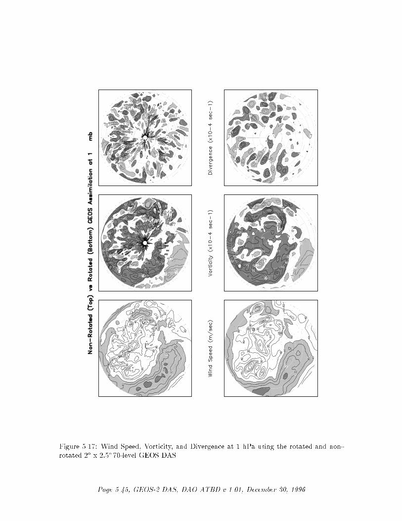
Figure 5.17: Wind Speed, Vorticity, and Divergence at 1 hPa using the rotated and non-
rotated 2� x 2:5� 70-level GEOS DAS.
Page 5.45, GEOS-2 DAS, DAO ATBD v 1.01, December 30, 1996

where qF is the quantity after application of the full Shapiro �lter, q is the un�ltered
quantity, and � is an adjustable time scale. Thus, a fraction �t�
of the full Shapiro �lter is
incorporated at each model timestep. In the GEOS-2 GCM, the time scale � is equal to 1.5
hours, and has been chosen so as to remove the two-grid interval wave in about six hours.
For the 2� x 2:5� x 70 level GEOS-2 GCM, an 8th-order Shapiro �lter is used below 10 hPa
and a 4th-order �lter above. The response function of the 8th-order �lter is shown in Figure
5.18. The GEOS-2 GCM also uses a high-latitude Fourier �lter to avoid linear instability
due to violation of the CFL condition for the Lamb wave and internal gravity waves near
the poles. This polar �lter is only applied to the time-tendencies of the prognostic �elds,
ie. winds, potential temperature, speci�c humidity, and surface pressure.
For the moisture equation, negative values computationally generated through advection
are �lled by \borrowing" from below while conserving the vertically integrated moisture,
ie.,
Z le�1
le+1�qdz
!final
=
Z le�1
le+1�qdz
!initial
: (5.113)
Using the hydrostatic relation ��z = � �pg= ��
g��, we may write
Z le�1
le+1�qd�
!final
=
Z le�1
le+1�qd�
!initial
: (5.114)
Approximating equaton (5.114) by
(�ql��l + �ql�1��l�1)final = (�ql��l + �ql�1��l�1)initial ; (5.115)
an expression for the updated moisture at level l is given by
�qlfinal =
��ql + �ql�1
��l�1
��l
�initial
���ql�1
��l�1
��l
�final
: (5.116)
Assuming that �ql�1 is initially negative, we require that its �nal value is set to zero.
Thus
�ql�1final = 0;
�qlfinal =
��ql + �ql�1
��l�1
��l
�initial
: (5.117)
This process is repeated until the lowest level is reached. If the resulting �qnlay is
negative, the mass-weighted speci�c humidity in the lowest model level is simply set to
zero.
Page 5.46, GEOS-2 DAS, DAO ATBD v 1.01, December 30, 1996

Figure 5.18: Shapiro �lter response function used in the 2� x 2:5�GEOS-2 GCM.
Page 5.47, GEOS-2 DAS, DAO ATBD v 1.01, December 30, 1996

5.3.3 Atmospheric Physics
5.3.3.1 Moist Convective Processes
5.3.3.1.1 Sub-grid and Large-scale Convection Sub-grid scale cumulus convection
is parameterized using the Relaxed Arakawa Schubert (RAS) scheme of Moorthi and Suarez
(1992), which is a linearized Arakawa Schubert type scheme. RAS predicts the mass ux
from an ensemble of clouds. Each subensemble is identi�ed by its entrainment rate and
level of neutral bouyancy which are determined by the grid-scale properties.
The thermodynamic variables that are used in RAS to describe the grid scale vertical
pro�le are the dry static energy, s = cpT + gz, and the moist static energy, h = cpT + gz +
Lq. The conceptual model behind RAS depicts each subensemble as a rising plume cloud,
entraining mass from the environment during ascent, and detraining all cloud air at the
level of neutral buoyancy. RAS assumes that the normalized cloud mass ux, �, normalized
by the cloud base mass ux, is a linear function of height, expressed as:
@�(z)
@z= � or
@�(P�)
@P�= �cp
g��
where we have used the hydrostatic equation written in the form:
@z
@P�= �cp
g�
The entrainment parameter, �, characterizes a particular subensemble based on its
detrainment level, and is obtained by assuming that the level of detrainment is the level of
neutral buoyancy, ie., the level at which the moist static energy of the cloud, hc, is equal to
the saturation moist static energy of the environment, h�. Following Moorthi and Suarez
(1992), � may be written as
� =hB � h�D
cpg
R PBPD
�(h�D � h)dP�;
where the subscript B refers to cloud base, and the subscript D refers to the detrainment
level.
The convective instability is measured in terms of the cloud work function A, de�ned
as the rate of change of cumulus kinetic energy. The cloud work function is related to
the buoyancy, or the di�erence between the moist static energy in the cloud and in the
environment:
A =
Z PB
PD
�
1 +
�hc � h�
P�
�dP�
where is Lcp
@q�
@Tobtained from the Claussius Clapeyron equation, and the subscript c
refers to the value inside the cloud.
To determine the cloud base mass ux, the rate of change of A in time due to dissipation
by the clouds is assumed to approximately balance the rate of change of A due to the
Page 5.48, GEOS-2 DAS, DAO ATBD v 1.01, December 30, 1996

generation by the large scale. This is the quasi-equilibrium assumption, and results in an
expression for mB:
mB =� dA
dt
���ls
K
where K is the cloud kernel, de�ned as the rate of change of the cloud work function
per unit cloud base mass ux, and is currently obtained by analytically di�erentiating the
expression for A in time. The rate of change of A due to the generation by the large scale
can be written as the di�erence between the current A(t + �t) and its equillibrated value
after the previous convective time step A(t), divided by the time step. A(t) is approximated
as some critical Acrit, computed by Lord (1982) from insitu observations.
The predicted convective mass uxes are used to solve grid-scale temperature and mois-
ture budget equations to determine the impact of convection on the large scale �elds of
temperature (through latent heating and compensating subsidence) and moisture (through
precipitation and detrainment):
@�
@t
����c
= �mB
cpP��@s
@p
and@q
@t
����c
= �mB
L�(@h
@p� @s
@p)
where � = TP� , P = (p=p0), and � is the relaxation parameter.
As an approximation to a full interaction between the di�erent allowable subensembles,
many clouds are simulated frequently, each modifying the large scale environment some
fraction � of the total adjustment. The parameterization thereby \relaxes" the large scale
environment towards equillibrium.
In addition to the RAS cumulus convection scheme, the GEOS-2 GCM employs a
Kessler-type scheme for the re-evaporation of falling rain (Sud and Molod, 1988), which
correspondingly adjusts the temperature assuming h is conserved. RAS in its current for-
mulation assumes that all cloud water is deposited into the detrainment level as rain. All
of the rain is available for re-evaporation, which begins in the level below detrainment. The
scheme accounts for some microphysics such as the rainfall intensity, the drop size distribu-
tion, as well as the temperature, pressure and relative humidity of the surrounding air. The
fraction of the moisture de�cit in any model layer into which the rain may re-evaporate is
controlled by a free parameter, which allows for a relatively e�cient re-evaporation of liquid
precipitate and larger rainout for frozen precipitation.
Due to the increased vertical resolution near the surface, the lowest model layers are
averaged to provide a 50 hPa thick sub-cloud layer for RAS. Each time RAS is invoked
(every ten simulated minutes), a number of randomly chosen subensembles are checked for
the possibility of convection, from just above cloud base to 10 hPa.
Supersaturation or large-scale precipitation is initiated in the GEOS GCM whenever the
relative humidity in any grid-box exceeds a critical value, currently 100 %. The large-scale
precipitation re-evaporates during descent to partially saturate lower layers in a process
identical to the re-evaporation of convective rain.
Page 5.49, GEOS-2 DAS, DAO ATBD v 1.01, December 30, 1996

5.3.3.1.2 Cloud Formation Convective and large-scale cloud fractons which are used
for cloud-radiative interactions are determined diagnostically as part of the cumulus and
large-scale parameterizations. Convective cloud fractions produced by RAS are proportional
to the detrained liquid water amount given by
FRAS = min
�lRAS
lc; 1:0
�
where lc is an assigned critical value equal to 1:25 g/kg. A memory is associated with
convective clouds de�ned by:
FnRAS = min
�FRAS + (1� �tRAS
�)Fn�1RAS ; 1:0
�
where FRAS is the instantanious cloud fraction and Fn�1RAS is the cloud fraction from the
previous RAS timestep. The memory coe�cient is computed using a RAS cloud timescale,
� , equal to 1 hour. RAS cloud fractions are cleared when they fall below 5 %.
Large-scale cloudiness is de�ned, following Slingo and Ritter (1985), as a function of
relative humidity:
FLS = min
"�RH �RHc
1�RHc
�2; 1:0
#
where
RHc = 1� s(1� s)(2�p3 + 2
p3 s)r
s = p=psurf
r =
�1:0� RHmin
�
�RHmin = 0:75
� = 0:573285:
These cloud fractions are suppressed, however, in regions where the convective sub-cloud
layer is conditionally unstable. The functional form of RHc is shown in Figure (5.19).
The total cloud fraction in a grid box is determined by the larger of the two cloud
fractions:
FCLD = max [FRAS ; FLS ] :
Finally, cloud fractions are time-averaged between calls to the radiation packages.
Page 5.50, GEOS-2 DAS, DAO ATBD v 1.01, December 30, 1996
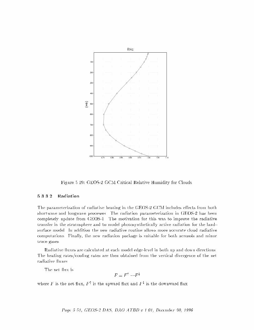
Figure 5.19: GEOS-2 GCM Critical Relative Humidity for Clouds.
5.3.3.2 Radiation
The parameterization of radiative heating in the GEOS-2 GCM includes e�ects from both
shortwave and longwave processes. The radiation parameterization in GEOS-2 has been
completely update from GEOS-1. The motivation for this was to improve the radiative
transfer in the stratosphere and to model photosynthetically active radiation for the land-
surface model. In addition the new radiative routine allows more accurate cloud radiative
computations. Finally, the new radiation package is suitable for both aerosols and minor
trace gases.
Radiative uxes are calculated at each model edge-level in both up and down directions.
The heating rates/cooling rates are then obtained from the vertical divergence of the net
radiative uxes.
The net ux is
F = F " � F #
where F is the net ux, F " is the upward ux and F # is the downward ux.
Page 5.51, GEOS-2 DAS, DAO ATBD v 1.01, December 30, 1996

The heating rate due to the divergence of the radiative ux is given by
@�cpT
@t= �@F
@z
or@T
@t=
g
cp�
@F
@�
where g is the acceleration due to gravity and cp is the heat capacity of air at constant
pressure.
The time tendency for Longwave Radiation is updated every 3 hours. The time tendency
for Shortwave Radiation is updated once every three hours assuming a normalized incident
solar radiation, and subsequently modi�ed at every model time step by the true incident
radiation. The solar constant value used in the GEOS-2 GCM is equal to 1365W=m2 and a
CO2 mixing ratio of 330 ppm. For the ozone mixing ratio, monthly mean zonally averaged
climatological values speci�ed as a function of latitude and height (Rosen�eld, et al., 1987)
are linearly interpolated to the current time. The GEOS-2 GCM also uses climatological
water vapor data above 100 hPa from the Stratospheric Aerosol and Gas
5.3.3.2.1 Shortwave Radiation The shortwave radiation package used in the GEOS-
2 GCM computes solar radiative heating due to the absoption by water vapor, ozone,
carbon dioxide, oxygen, clouds, and aerosols and due to the scattering by clouds, aerosols,
and gases. The shortwave radiative processes are described by Chou (1990,1992). This
shortwave package uses the Delta-Eddington approximation to compute the bulk scattering
properties of a single layer following King and Harshvardhan (1986). The transmittance
and re ectance of di�use radiation follow the procedures of Sagan and Pollock (1967) and
Lacis and Hansen (1974).
Highly accurate heating rate calculations are obtained through the use of an optimal
grouping strategy of spectral bands. By grouping the UV and visible regions as indicated
in Table 5.3, the Rayleigh scattering and the ozone absorption of solar radiation can be
accurately computed in the ultraviolet region and the photosynthetically active radiation
(PAR) region. The computation of solar ux in the infrared region is performed with a
broadband parameterization using the spectrum regions shown in Table 5.4. The solar
radiation algorithm used in the GEOS-2 GCM can be applied not only for climate studies
but also for studies on the photolysis in the upper atmosphere and the photosynthesis in
the biosphere.
Within the shortwave radiation package, both ice and liquid cloud particles are allowed
to co-exist in any of the model layers. Two sets of cloud parameters are used, one for ice
paticles and the other for liquid particles. Cloud parameters are de�ned as the cloud optical
thickness and the e�ective cloud particle size. In the GEOS-2 GCM, the e�ective radius
for water droplets is given as 10 microns, while 65 microns is used for ice particles. The
absorption due to aerosols is currently set to zero.
To simplify calculations in a cloudy atmosphere, clouds are grouped into low (p > 700
hPa), middle (700 hPa � p > 400 hPa), and high (p < 400 hPa) cloud regions. Within
each of the three regions, clouds are assumed maximally overlapped, and the cloud cover of
the group is the maximum cloud cover of all the layers in the group. The optical thickness
Page 5.52, GEOS-2 DAS, DAO ATBD v 1.01, December 30, 1996

UV and Visible Spectral Regions
Region Band Wavelength (micron)
UV-C 1. .175 - .225
2. .225 - .245
.260 - .280
3. .245 - .260
UV-B 4. .280 - .295
5. .295 - .310
6. .310 - .320
UV-A 7. .320 - .400
PAR 8. .400 - .700
Table 5.3: UV and Visible Spectral Regions used in shortwave radiation package.
Infrared Spectral Regions
Band Wavenumber(cm�1) Wavelength (micron)
1 1000-4400 2.27-10.0
2 4400-8200 1.22-2.27
3 8200-14300 0.70-1.22
Table 5.4: Infrared Spectral Regions used in shortwave radiation package.
of a given layer is then scaled for both the direct (as a function of the solar zenith angle)
and di�use beam radiation so that the grouped layer re ectance is the same as the original
re ectance. The solar ux is computed for each of the eight cloud realizations possible
within this low/middle/high classi�cation, and appropriately averaged to produce the net
solar ux.
5.3.3.2.2 Longwave Radiation The longwave radiation package used in the GEOS-2
GCM is thoroughly described by Chou and Suarez (1994). As described in that document,
IR uxes are computed due to absorption by water vapor, carbon dioxide, and ozone. The
spectral bands together with their absorbers and parameterization methods, con�gured for
the GEOS-2 GCM, are shown in Table 5.5.
The longwave radiation package accurately computes cooling rates for the middle and
lower atmosphere from 0.01 hPa to the surface. Errors are < 0.4 C day�1 in cooling rates
and < 1% in uxes. From Chou and Suarez, it is estimated that the total e�ect of neglecting
all minor absorption bands and the e�ects of minor infrared absorbers such as nitrous oxide
(N2O), methane (CH4), and the chloro uorocarbons (CFCs), is an underestimate of � 5
W/m2 in the downward ux at the surface and an overestimate of � 3 W/m2 in the upward
ux at the top of the atmosphere.
Similar to the procedure used in the shortwave radiation package, clouds are grouped
into three regions catagorized as low/middle/high. The net clear line-of-site probability (P )
between any two levels, p1 and p2 (p2 > p1), assuming randomly overlapped cloud groups,
is simply the product of the probabilities within each group:
Page 5.53, GEOS-2 DAS, DAO ATBD v 1.01, December 30, 1996

IR Spectral Bands
Band Spectral Range (cm�1) Absorber Method
1 0-340 H2O line T
2 340-540 H2O line T
3a 540-620 H2O line K
3b 620-720 H2O continuum S
3b 720-800 CO2 T
4 800-980 H2O line K
H2O continuum S
H2O line K
5 980-1100 H2O continuum S
O3 T
6 1100-1380 H2O line K
H2O continuum S
7 1380-1900 H2O line T
8 1900-3000 H2O line K
K: k-distribution method with linear pressure scaling
T: Table look-up with temperature and pressure scaling
S: One-parameter temperature scaling
Table 5.5: IR Spectral Bands, Absorbers, and Parameterization Method (from Chou and
Suarez, 1994)
Pnet = Plow � Pmid � Phi:
Since all clouds within a group are assumed maximally overlapped, the clear line-of-site
probability within a group is given by:
Pgroup = 1� Fmax;
where Fmax is the maximum cloud fraction encountered between p1 and p2 within that
group. For groups and/or levels outside the range of p1 and p2, a clear line-of-site probability
equal to 1 is assigned.
5.3.3.2.3 Cloud-Radiation Interaction The cloud fractions and diagnosed cloud liq-
uid water produced by moist processes within the GEOS-2 GCM are used in the radiation
packages to produce cloud-radiative forcing. The cloud optical thickness associated with
large-scale cloudiness is made proportional to the diagnosed large-scale liquid water, `, de-
trained due to super-saturation. Two values are used corresponding to cloud ice particles
and water droplets. The range of optical thickness for these clouds is given as
0:0002 � �ice(hPa�1) � 0:002 for 0 � ` � 2 mg/kg;
0:02 � �h2o(hPa�1) � 0:2 for 0 � ` � 10 mg/kg:
Page 5.54, GEOS-2 DAS, DAO ATBD v 1.01, December 30, 1996
The partitioning, �, between ice particles and water droplets is achieved through a linear
scaling in temperature:
0 � � � 1 for 233:15 � T � 253:15:
The resulting optical depth associated with large-scale cloudiness is given as
�LS = ��h2o + (1� �)�ice:
The optical thickness associated with sub-grid scale convective clouds produced by RAS
is given as
�RAS = 0:16 hPa�1:
The total optical depth in a given model layer is computed as a weighted average between
the large-scale and sub-grid scale optical depths, normalized by the total cloud fraction in
the layer:
� =
�FRAS �RAS + FLS �LS
FRAS + FLS
��p;
where FRAS and FLS are the time-averaged cloud fractions associated with RAS and
large-scale processes described in Section 5.3.3.1.2. The optical thickness for the longwave
radiative feedback is assumed to be 75 % of these values.
The entire Moist Convective Processes Module is called with a frequency of 10 minutes.
The cloud fraction values are time-averaged over the period between Radiation calls (every
3 hours). Therefore, in a time-averaged sense, both convective and large-scale cloudiness
can exist in a given grid-box.
5.3.3.3 Turbulence
Turbulence is parameterized in the GEOS-2 GCM to account for its contribution to the
vertical exchange of heat, moisture, and momentum. The turbulence scheme is invoked
every 30 minutes, and employs a backward-implicit iterative time scheme with an internal
time step of 5 minutes. The tendencies of atmospheric state variables due to turbulent
di�usion are calculated using the di�usion equations:
@u
@t turb=
@
@z(�u0w0) = @
@z(Km
@u
@z)
@v
@t turb=
@
@z(�v0w0) = @
@z(Km
@v
@z)
@T
@t= P�
@�
@t turb= P�
@
@z(�w0�0) = P�
@
@z(Kh
@�v
@z)
@q
@t turb=
@
@z(�w0q0) = @
@z(Kh
@q
@z)
Page 5.55, GEOS-2 DAS, DAO ATBD v 1.01, December 30, 1996

Within the atmosphere, the time evolution of second turbulent moments is explicitly
modeled by representing the third moments in terms of the �rst and second moments. This
approach is known as a second-order closure modeling. To simplify and streamline the
computation of the second moments, the level 2.5 assumption of Mellor and Yamada (1974)
and Yamada (1977) is employed, in which only the turbulent kinetic energy (TKE),
1
2q2 =
1
2
hu02 + v02 + w02
i;
is solved prognostically and the other second moments are solved diagnostically. The
prognostic equation for TKE allows the scheme to simulate some of the transient and
di�usive e�ects in the turbulence. The TKE budget equation is solved numerically using
an implicit backward computation of the terms linear in q2 and is written:
d
dt(1
2q2)� @
@z(5
3�1q
@
@z(1
2q2)) = �u0w0@U
@z� v0w0
@V
@z+
g
�0w0�v
0 � q3
�1
where q is the turbulent velocity, u0, v0, w0 and �0 are the uctuating parts of the velocity
components and potential temperature, U and V are the mean velocity components, �0�1
is the coe�cient of thermal expansion, and �1 and �1 are constant multiples of the master
length scale, `, which is designed to be a characteristic measure of the vertical structure of
the turbulent layers.
The �rst term on the left-hand side represents the time rate of change of TKE, and
the second term is a representation of the triple correlation, or turbulent transport term.
The �rst three terms on the right-hand side represent the sources of TKE due to shear and
bouyancy, and the last term on the right hand side is the dissipation of TKE.
In the level 2.5 approach, the vertical uxes of the scalars �v and q and the wind compo-
nents u and v are expressed in terms of the di�usion coe�cients Kh and Km, respectively.
In the statisically realizable level 2.5 turbulence scheme of Helfand and Labraga (1988),
these di�usion coe�cients are expressed as
Kh =
(q ` SH(GM ; GH) for decaying turbulenceq2
qe` SH(GMe ; GHe) for growing turbulence
and
Km =
(q ` SM(GM ; GH) for decaying turbulenceq2
qe` SM(GMe; GHe) for growing turbulence
where the subscript e refers to the value under conditions of local equillibrium (obtained
from the Level 2.0 Model), ` is the master length scale related to the vertical structure of
the atmosphere, and SM and SH are functions of GH and GM , the dimensionless buoyancy
and wind shear parameters, respectively. Both GH and GM , and their equilibrium values
GHe and GMe , are functions of the Richardson number:
Page 5.56, GEOS-2 DAS, DAO ATBD v 1.01, December 30, 1996

RI =
g�v@�v@z
(@u@z)2 + (@v
@z)2
=cp@�v@z
@P�
@z
(@u@z)2 + (@v
@z)2:
Negative values indicate unstable buoyancy and shear, small positive values (< 0:2)
indicate dominantly unstable shear, and large positive values indicate dominantly stable
strati�cation.
Turbulent eddy di�usion coe�cients of momentum, heat and moisture in the surface
layer, which corresponds to the lowest GCM level (see 5.2), are calculated using stability-
dependant functions based on Monin-Obukhov theory:
Km(surface) = Cu � u� = CDWs
and
Kh(surface) = Ct � u� = CHWs
where u� = CuWs is the surface friction velocity, CD is termed the surface drag coe�cient,
CH the heat transfer coe�cient, and Ws is the magnitude of the surface layer wind.
Cu is the dimensionless exchange coe�cient for momentum from the surface layer simi-
larity functions:
Cu =u�
Ws=
k
m
where k is the von Karman constant and m is the surface layer non-dimensional wind shear
given by
m =
Z �
�0
�m
�d�:
Here � is the non-dimensional stability parameter, and �m is the similarity function of �
which expresses the stability dependance of the momentum gradient. The functional form
of �m is speci�ed di�erently for stable and unstable layers.
Ct is the dimensionless exchange coe�cient for heat and moisture from the surface layer
similarity functions:
Ct = �(w0�0)
u���= �(w0q0)
u��q=
k
( h + g)
where h is the surface layer non-dimensional temperature gradient given by
h =
Z �
�0
�h
�d�:
Here �h is the similarity function of �, which expresses the stability dependance of the
temperature and moisture gradients, and is speci�ed di�erently for stable and unstable
layers according to Helfand and Schubert, 1995.
g is the non-dimensional temperature or moisture gradient in the viscous sublayer,
which is the mosstly laminar region between the surface and the tops of the roughness
elements, in which temperature and moisture gradients can be quite large. Based on Yaglom
and Kader (1974):
g =0:55(Pr2=3� 0:2)
�1=2(h0u� � h0refu�ref )
1=2
Page 5.57, GEOS-2 DAS, DAO ATBD v 1.01, December 30, 1996

where Pr is the Prandtl number for air, � is the molecular viscosity, z0 is the surface
roughness length, and the subscript ref refers to a reference value. h0 = 30z0 with a
maximum value over land of 0.01
The surface roughness length over oceans is is a function of the surface-stress velocity,
z0 = c1u3�+ c2u
2�+ c3u� + c4 +
c5
u�
where the constants are chosen to interpolate between the reciprocal relation of Kondo(1975)
for weak winds, and the piecewise linear relation of Large and Pond(1981) for moderate to
large winds. Roughness lengths over land are speci�ed from the climatology of Dorman and
Sellers (1989).
For an unstable surface layer, the stability functions, chosen to interpolate between the
condition of small values of � and the convective limit, are the KEYPS function (Panofsky,
1973) for momentum, and its generalization for heat and moisture:
�m4 � 18��m
3 = 1 ; �h2 � 18��h
3 = 1 :
The function for heat and moisture assures non-vanishing heat and moisture uxes as the
wind speed approaches zero.
For a stable surface layer, the stability functions are the observationally based functions
of Clarke (1970), slightly modi�ed for the momemtum ux:
�m =1 + 5�1
1 + 0:00794�1(1 + 5�1); �h =
1+ 5�1
1 + 0:00794�(1+ 5�1):
The moisture ux also depends on a speci�ed evapotranspiration coe�cient, set to unity
over oceans and dependant on the climatological ground wetness over land.
Once all the di�usion coe�cients are calculated, the di�usion equations are solved nu-
merically using an implicit backward operator.
5.3.3.3.1 Atmospheric Boundary Layer The depth of the atmospheric boundary
layer (ABL) is diagnosed by the parameterization as the level at which the turbulent kinetic
energy is reduced to a tenth of its maximum near surface value. The vertical structure of
the ABL is explicitly resolved by the lowest few (3-8) model layers.
5.3.3.3.2 Surface Energy Budget The ground temperature equation is solved as part
of the turbulence package using a backward implicit time di�erencing scheme:
Cg@Tg
@t= Rsw �Rlw +Qice �H � LE
where Rsw is the net surface downward shortwave radiative ux and Rlw is the net surface
upward longwave radiative ux.
H is the upward sensible heat ux, given by:
H = P��cpCHWs(�surface � �NLAY ) where : CH = CuCt
Page 5.58, GEOS-2 DAS, DAO ATBD v 1.01, December 30, 1996

where � = the atmospheric density at the surface, cp is the speci�c heat of air at constant
pressure, and � represents the potential temperature of the surface and of the lowest �-level,
respectively.
The upward latent heat ux, LE, is given by
LE = ��LCHWs(qsurface � qNLAY ) where : CH = CuCt
where � is the fraction of the potential evapotranspiration actually evaporated, L is the
latent heat of evaporation, and qsurface and qNLAY are the speci�c humidity of the surface
and of the lowest �-level, respectively.
The heat conduction through sea ice, Qice, is given by
Qice =Cti
Hi
(Ti � Tg)
where Cti is the thermal conductivity of ice, Hi is the ice thickness, assumed to be 3m
where sea ice is present, Ti is 273 degrees Kelvin, and Tg is the surface temperature of the
ice.
Cg is the total heat capacity of the ground, obtained by solving a heat di�usion equation
for the penetration of the diurnal cycle into the ground (Blackadar, 1977), and is given by:
Cg =
s�Cs
2!=
r(0:386+ 0:536W + 0:15W 2)2� 10�3
86400
2�:
Here, the thermal conductivity, �, is equal to 2 � 10�3 lysec
cmoK
, the angular velocity of the
earth, !, is written as 86400 sec=day divided by 2� radians=day, and the expression for
Cs, the heat capacity per unit volume at the surface, is a function of the ground wetness,
W .
5.3.3.4 Gravity Wave Drag
A gravity wave drag scheme has been added to the GEOS-2 GCM. This provides a physically-
based momentum dissipation in the model. The gravity wave drag was added primarily to
address excessive zonality of tropospheric winds. The scheme has a dramatic positive impact
on sea level pressure and tropospheric momentum and heat uxes. Gravity wave processes
in the stratosphere and mesosphere require further development of the scheme.
The GEOS-2 GCM employs the gravity wave drag scheme of Zhou et al. (1996). This
scheme is a modi�ed version of Vernekar et al. (1992), which was based on Alpert et al.
(1988) and Helfand et al. (1987). In this version, the gravity wave stress at the surface is
based on that derived by Pierrehumbert (1986) and is given by:
j~�sfcj =�U3
N`�
F 2r
1 + F 2r
!; (5.118)
where Fr = Nh=U is the Froude number, N is the Brunt - V�ais�al�a frequency, U is the
surface wind speed, h is the standard deviation of the sub-grid scale orography, and `� is
Page 5.59, GEOS-2 DAS, DAO ATBD v 1.01, December 30, 1996

the wavelength of the monochromatic gravity wave in the direction of the low-level wind. A
modi�cation introduced by Zhou et al. allows for the momentum ux to escape through the
top of the model, although this e�ect is small for the current 70-level model. The subgrid
scale standard deviation is de�ned by h, and is not allowed to exceed 400 m.
The e�ects of using this scheme within the GEOS GCM are shown in Takacs and Suarez
(1996). Experiments using the gravity wave drag parameterization yielded signi�cant and
bene�cial impacts on both the time-mean ow and the transient statistics of the GEOS
GCM climatology, and have eliminated most of the worst dynamically driven biases in the
GEOS-1 GCM simulation. An examination of the angular momentum budget during climate
runs indicates that the resulting gravity wave torque is similar to the data-driven torque
introduced by the GEOS-1 DAS analysis which was performed without gravity wave drag. It
was shown that the inclusion of gravity wave drag results in large changes in both the mean
ow and in eddy uxes. The result is a more accurate simulation of surface stress (through
a reduction in the surface wind strength), of mountain torque (through a redistribution of
mean sea-level pressure), and of momentum convergence (through a reduction in the ux
of westerly momentum by transient ow eddies).
5.3.4 Boundary Conditions and other Input Data
Development and maintenance of boundary condition data sets is a major task. Improve-
ment of some boundary condition data sets is required to accommodate the land-surface
model. Increased exibility to use di�erent boundary data sets, perhaps prescribed directly
from MTPE observations is also required. Finally, much of the work of future development
is to make some of the current boundary condition data sets interactive. This allows even
more model degrees of freedom which must be properly de�ned.
Required �elds which are not explicitly predicted or diagnosed during model execution
must either be prescribed internally or obtained from external data sets. In the GEOS-2
GCM these �elds include the boundary conditions: surface geopotential, surface geopo-
tential variance, vegetation index, sea surface temperature, ground wetness, sea ice, snow,
surface roughness and surface albedo, and the radiation-related background levels of: ozone,
carbon dioxide, and stratospheric moisture.
Boundary condition data sets are available at the model's 4� x 5� and 2� x 2:5� resolutions
for either climatological or yearly varying conditions. Any frequency of boundary condition
data can be used in the GEOS-2 GCM; however, the current selection of data is summa-
rized in Table 5.6. The time mean values are interpolated during each model timestep to
the current time. Future model versions will incorporate boundary conditions at higher
spatial (1� x 1�) resolutions.
5.3.4.1 Topography and Topography Variance
Surface geopotential heights are provided from an averaging of the Navy 10 minute by
10 minute dataset supplied by the National Center for Atmospheric Research (NCAR) to
the model's grid resolution. The original topography is �rst rotated to the proper grid-
orientation which is being run, and then averages the data to the model resolution. The
averaged topography is then passed through a Lanczos (1966) �lter in both dimensions
Page 5.60, GEOS-2 DAS, DAO ATBD v 1.01, December 30, 1996

GEOS-2 GCM Input Datasets
Variable Frequency Years
Ground Wetness monthly 1979-1992, climatology
Sea Ice Extent monthly 1979-1992, climatology
Sea Ice Extent weekly 1982-1992, climatology
Sea Surface Temperature monthly 1979-1992, climatology
Sea Surface Temperature weekly 1982-1995, climatology
Snow Extent monthly climatology
Snow Extent weekly 1982-1992, climatology
Zonally Averaged Upper-Level Moisture monthly climatology
Zonally Averaged Ozone Concentration monthly climatology
Table 5.6: Boundary conditions and other input data used in the GEOS-2 GCM. Also noted
are the current years and frequencies available.
which removes the smallest scales while inhibiting Gibbs phenomena.
In one dimension, we may de�ne a cyclic function in x as:
f(x) =a0
2+
NXk=1
(ak cos(kx) + bk sin(kx)) (5.119)
where N = IM2 and IM is the total number of points in the x direction. De�ning �x = 2�
IM ,
we may de�ne the average of f(x) over a 2�x region as:
f(x) =1
2�x
Z x+�x
x��xf(x0)dx0 (5.120)
Using equation (5.119) in equation (5.120) and integrating, we may write:
f(x) =a0
2+
1
2�x
NXk=1
"aksin(kx0)
k
�x+�x
x��x� bk
cos(kx0)
k
�x+�x
x��x
#(5.121)
or
f(x) =a0
2+
NXk=1
sin(k�x)
k�x(ak cos(kx) + bk sin(kx)) (5.122)
Thus, the Fourier wave amplitudes are simply modi�ed by the Lanczos �lter response
functionsin(k�x)k�x . This may be compared with an mth-order Shapiro (1970) �lter response
function, de�ned as 1� sinm(k�x2 ), shown in Figure 5.20. It should be noted that negative
values in the topography resulting from the �ltering procedure are not �lled.
The standard deviation of the subgrid-scale topography is computed from a modi�ed
version of the the Navy 10 minute by 10 minute dataset. The 10 minute by 10 minute
Page 5.61, GEOS-2 DAS, DAO ATBD v 1.01, December 30, 1996

Figure 5.20: Comparison between the Lanczos and mth-order Shapiro �lter response func-
tions for m = 2, 4, and 8.
Page 5.62, GEOS-2 DAS, DAO ATBD v 1.01, December 30, 1996

GEOS-2 GCM Surface Type Designation
Type Vegetation Designation
1 Broadleaf Evergreen Trees
2 Broadleaf Deciduous Trees
3 Needleleaf Trees
4 Ground Cover
5 Broadleaf Shrubs
6 Dwarf Trees (Tundra)
7 Bare Soil
8 Desert (Bright)
9 Glacier
10 Desert (Dark)
100 Ocean
Table 5.7: GEOS-2 GCM surface type designations used to compute surface roughness (over
land) and surface albedo.
topography is passed through a wavelet �lter in both dimensions which removes the scale
smaller than 20 minutes. The topography is then averaged to 1�x1� grid resolution, and
then re-interpolated back to the 10 minute by 10 minute resolution. The sub-grid scale
variance is constructed based on this smoothed dataset.
5.3.4.2 Surface Type
GEOS-2 GCM Surface Types are designated using the Koster-Suarez (1992) mosaic phi-
losophy which allows multiple \tiles", or multiple surface types, in any one grid cell. The
Koster-Suarez Land Surface Model (LSM) surface type classi�cations are shown in Table
5.7. The surface types and the percent of the grid cell occupied by any surface type were
derived from the surface classi�cation of Defries and Townshend (1994), and information
about the location of permanent ice was obtained from the classi�cations of Dorman and
Sellers (1989). The surface designation at 1�x1� resolution is shown in Figure 5.21. The
determination of the land or sea category of surface type was made from NCAR's 10 minute
by 10 minute Navy topography dataset, which includes information about the percentage of
water-cover at any point. The data were averaged to the model's 4� x 5� and 2� x 2:5� grid
resolutions, and any grid-box whose averaged water percentage was � 60% was de�ned as
a water point. The 4� x 5� grid Land-Water designation was further modi�ed subjectively
to ensure su�cient representation from small but isolated land and water regions.
5.3.4.3 Sea Surface Temperature
Yearly varying monthly mean sea surface temperatures for the 4� x 5� grid resolution are
from AMIP speci�ed monthly mean �elds (Gates, 1992). All other monthly varying data sets
were interpolated from data of Reynolds (1988). The weekly varying data was provided by
the National Centers for Environmental Prediction (NCEP) using an optimum interpolation
sea surface temperature analysis (Reynolds and Smith, 1994)with bias correction (Reynolds,
Page 5.63, GEOS-2 DAS, DAO ATBD v 1.01, December 30, 1996

Figure 5.21: GEOS-2 GCM Surface Type Compinations at 2� x 2:5� resolution.
Page 5.64, GEOS-2 DAS, DAO ATBD v 1.01, December 30, 1996
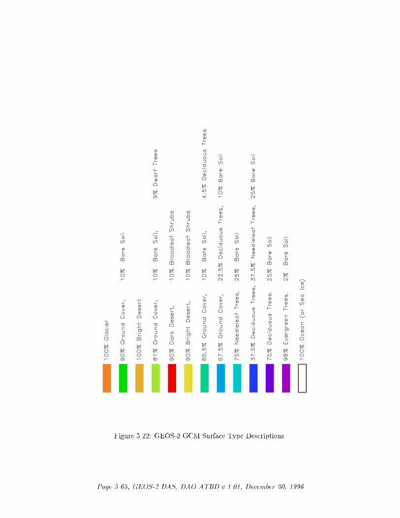
Figure 5.22: GEOS-2 GCM Surface Type Descriptions.
Page 5.65, GEOS-2 DAS, DAO ATBD v 1.01, December 30, 1996

1988; Reynolds and Marsico, 1993). The satellite data were provided by the National
Environmental Satellite, Data and Information Service (NESDIS). During 1981-1989, the
in situ data was obtained from the Comprehensive Ocean Atmosphere Data Set (COADS)
(Slutz, et al., 1985; Woodru�, et al., 1993). For 1990-1995, the in situ data was obtained
from radio messages carried on the Global Telecommunication System. A binomial time
�lter of (14; 12; 14) was applied to the weekly data as well as a minimum temperature limit of
271.36K.
5.3.4.4 Surface Roughness
The surface roughness length over oceans is computed iteratively with the wind stress by the
surface layer parameterization (Helfand and Schubert, 1995). It employs an interpolation
between the functions of Large and Pond (1981) for high winds and of Kondo (1975) for
weak winds.
5.3.4.5 Albedo
The surface albedo computation, described in Koster and Suarez (1991), employs the \two
stream" approximation used in Sellers' (1987) Simple Biosphere (SiB) Model which dis-
tinguishes between the direct and di�use albedos in the visible and in the near infra-red
spectral ranges. The albedos are functions of the observed leaf area index (a description
of the relative orientation of the leaves to the sun), the greenness fraction, the vegetation
type, and the solar zenith angle. Modi�cations are made to account for the presence of
snow, and its depth relative to the height of the vegetation elements.
5.3.4.6 Sea Ice
Monthly mean sea ice extents were interpolated to the model's 4� x 5� and 2� x 2:5� grid
resolutions from the AMIP monthly mean �elds (Gates, 1992). The weekly sea ice ex-
tent data, originally from the Navy/NOAA Joint Ice Center (Reynolds and Smith, 1994),
were provided by NCEP at a 2� x 2� resolution. The data were then interpolated to the
4� x 5� and 2� x 2:5� grid resolutions consistent with the GEOS-2 GCM land/water mask.
Sea ice thickness is assumed to be three meters and is used in the calculation of conduction
through sea ice accounted for in the surface energy budget. Note that unlike the GEOS-1
GCM, the permanent Ross and Ronne ice shelves of Antartica were not included in the
vegetation data set which de�nes glacier extent; therefore, the marine ice shelves have been
classi�ed as sea ice.
5.3.4.7 Snow Cover
The monthly mean snow extent is based on climatological albedo values which are greater
than 0.4 (Posey and Clapp, 1964; Kitzmiller, personal communication). The climatological
monthly mean data set was created to reproduce the snow extent used in GEOS-1. The
weekly snow extent data were provided by NCEP at a 2� x 2� grid resolution (Dewey and
Heim, 1981) and were interpolated to the 4� x 5� and 2� x 2:5� grid resolutions consistent
Page 5.66, GEOS-2 DAS, DAO ATBD v 1.01, December 30, 1996

with the GEOS-2 GCM land/water mask. A binomial (14 ;12 ;
14) time �lter was applied to the
weekly snow extent data. Also, a persistant block of snow from 46N-56N and 70E-92E which
resembled a misplaced plateau of Tibet was removed when neighboring grid-boxes were free
of snow. Snow depth is assumed to be a constant and set equal to a water equivalent of 50
mm. Snow amounts are used in the GEOS-2 GCM in the calculation of albedo and surface
conductive characteristics.
5.3.4.8 Upper Level Moisture
The GEOS-2 GCM uses climatological water vapor data above 100 hPa from the Strato-
spheric Aerosol and Gas Experiment (SAGE) as input into the model's radiation packages.
The SAGE data is archived as monthly zonal means at 5� latitudinal resolution. The
data is interpolated to the model's grid location and current time, and blended with the
GCM's moisture data. Below 300 hPa, the model's moisture data is used. Above 100 hPa,
the SAGE data is used. Between 100 and 300 hPa, a linear interpolation (in pressure) is
performed using the data from SAGE and the GCM.
5.3.4.9 Ground Temperature and Moisture
Ground temperature over land is predicted from a surface energy balance equation. The
ground wetness used in the GEOS-2 GCM is obtained from the monthly estimates of
Schemm, et al. (1992) based on the procedure developed by Mintz and Sera�ni (1984)
using an inverted single layer \bucket" model together with observed �elds of surface air
temperature and precipitation.
Page 5.67, GEOS-2 DAS, DAO ATBD v 1.01, December 30, 1996

5.4 Combining model and analysis: the IAU process
The IAU procedure was introduced in Chapter 4. It is an integral part of the GEOS-DAS,
smoothly integrating the information from the model and the analysis. Its use has been
controversial. The IAU process has also been confused with linear nudging techniques. This
section establishes the theoretical basis of the IAU, clari�es the relation with linear nudging,
and gives an example of performance enhancements achieved by the IAU.
The intermittent insertion of analyses has been the most commonly used strategy for
operational data assimilation. This approach typically begins with a statistical interpolation
scheme (such as OI or PSAS) that combines observations in a 6-hour time window with
a 6 hour model forecast to produce an analysis. This analysis is then used as an initial
condition for the next 6 hour forecast, and so on. Two related problems arise with the
intermittent approach: shocks to the model and data rejection. Sudden localized changes
to GCM �elds can spur large non-physical adjustment processes, the result of which can
be the unnecessary diminution of the e�ect of valid observations. For example, a large,
localized change to a model's mass �eld will likely produce (in mid-latitudes) a geostrophic
adjustment in which the change to the mass �eld would then largely disappear in the form
of gravity waves radiating away from the analysis location.
forecast
forecast
forecast
Analysis
Analysis
IAU
IAU
AnalysisIAU
18Z15Z12Z09Z06Z03Z
Figure 5.23: Schematic of the incremental analysis update (IAU) scheme employed in the GEOSDAS. Statistical analyses (OI or PSAS) are performed at synoptic times (0000, 0600, 1200 and 1800UTC). The assimilation is restarted three hours prior to the analysis time (heavy dashed lines), andthe model is integrated forward for 6 hours using the analysis increments as constant forcing (datain uence shown by shaded regions). At the end of the IAU interval, an un-forced forecast is made(dotted line) to provide the �rst guess for the next analysis.
Page 5.68, GEOS-2 DAS, DAO ATBD v 1.01, December 30, 1996

There have been a number of strategies for coping with the problems inherent in inter-
mittent assimilation: damped time-di�erencing schemes in the forecast model, initialization
methods, and balance constraints. A former version of the Goddard Laboratory for Atmo-
spheres (GLA) data assimilation system used a Matsuno time-di�erencing scheme (cf. Baker
et al., 1987), which damps high frequency oscillations. Even with this high-frequency damp-
ing the previous GLA system still su�ered from shocks and unrealistic precipitation (ex-
amples of which will be shown in below). Further elaborations of this approach, using dy-
namical initialization techniques, have been explored in Fox-Rabinovitz and Gross (1993)
and Fox-Rabinovitz (1995). Operational centers have made frequent use of normal mode
initialization methods. While quite e�ective at eliminating imbalances, these initialization
methods (even diabatic methods) tend to have unwanted side-e�ects on physical processes,
such as the loss of divergent wind structures in the tropics (Puri, 1985). In addition, such
methods make non-local changes to the analyses, most notably in areas where there were
no data. The NCEP SSI system (Parrish and Derber 1992) uses a linear balance constraint
as well as a non-linear pressure tendency constraint as integral parts of variational analysis
system.
The Incremental Analysis Updating (IAU) approach combines aspects of the intermittent
and continuous data assimilation approaches. A statistical analysis is performed intermit-
tently every 6 hours but used as a continuous forcing for the model prognostic variables
as illustrated in Fig. 5.23. Analysis increments are computed in a conventional way at the
analysis times (00, 06, 12, 18 UTC) by an analysis scheme such as PSAS or OI. These
increments are then inserted gradually into the model by restarting the short-term forecast
that provided the analysis background and adding a fraction of the analysis increment at
each model time-step. Over the six hour period centered on the analysis time, the full
e�ect of the analysis increment is realized. The �nal assimilation product thus e�ectively
consists of a model forecast produced using additional heat, momentum, moisture and mass
tendency terms which are updated every six hours from observations. This update scheme
for the assimilation is similar to the way the forcing tendencies from the model's physical
parameterizations and �lters are recomputed intermittently (usually every 30 minutes) and
gradually introduced into the ongoing integration at every time-step (section 5.3).
For an assimilation system to be used for climate and chemistry applications the IAU also
o�ers a set of particular advantages. In traditional numerical weather prediction schemes
precipitation and other diagnostic products are usually derived from multi-hour forecast.
These diagnostics are accumulated after discarding the �rst few hours of the forecast when
more severe spin-up processes take place. In the IAU, precipitation and other diagnostic
products are computed from a continuous model integration; therefore, closer to the actual
data time. In addition, because of its continuous nature, there can be frequent output of
diagnostics. This has proven useful for archiving surface products every hour (on request)
and is the reason the GEOS DAS can produce the special sub-orbital data sets requested by
AM-1 instrument teams. Finally, with the analysis increments archived, it is possible to re-
generate the assimilation products with additional diagnostics or increased time frequency,
for only the computational cost of the model simulation.
Although similar in nature, IAU di�ers from the UKMO Analysis Correction scheme
(Lorenc et al. 1991) in one important respect: IAU uses one analysis as assimilation forcing
while the UKMO system reanalyzes the data continuously through a 6 hour period. There
is also an important di�erence between IAU and the usual Newtonian nudging procedure
Page 5.69, GEOS-2 DAS, DAO ATBD v 1.01, December 30, 1996

(Anthes 1974; Stau�er and Seaman 1990): IAU forcing terms are held constant over the
insertion period, while in Newtonian nudging the forcing terms are proportional to the
changing di�erence between a target analysis and the instantaneous current model state;
this di�erence in forcing terms result in much di�erent �ltering properties (Bloom et a. 1996;
see also next subsection).
Signi�cant improvements in terms of assimilation accuracy, noise control, and the hy-
drological cycle spin-up are obtained using the IAU technique (Bloom et al. 1996). These
results are summarized in subsections 5.4.1|5.4.2. Details of the model/analysis interface
are given in subsection 5.4.3.
0 6 12 18 24 30 36 42 48Wave Period (hours)
0.0
0.2
0.4
0.6
0.8
1.0
1.2
rho
AMPLITUDE OF IAU RESPONSE FUNCTION
Neutral 6 hour growth rate12 hour growth rate
a
Figure 5.24: Amplitude of the IAU response function as a function of the disturbance period
in hours. Results are shown for 3 values of the growth/decay rate, � = 0 (neutral case,
solid), 1=� = 12 hours (dashed) and 1=� = 6 hours (dotted). See Bloom et al. 1996 for
details.
5.4.1 Filtering properties of IAU
Bloom et al. (1996) derive the linear response functions associated with the assimilation of
analysis increments into a generic linear model. Such an analysis of various assimilation ap-
proaches (intermittent, IAU, and dynamical relaxation or \nudging") within the context of
a linear system does give an indication of the behavior of these methods in a full assimilation
system. A number of important conclusions can be drawn from this linear analysis:
Page 5.70, GEOS-2 DAS, DAO ATBD v 1.01, December 30, 1996

Figure 5.25: Surface Pressure Tendency traces at a gridpoint over North America, results displayedfrom every time-step over the course of a 1-day assimilation: IAU (heavy solid); no IAU (light solid);model forecast, no data assimilation heavy dashed).
� In the linear system, IAU acts only on the contribution to the assimilation state by
the analysis increments. This is a con�rmation of one of the design goals of IAU; that
the process should not make any changes to the background state where there were
no data.
� The response function amplitude (IAU response compared to intermittent assimilation
response), Figure 5.24, indicates that the 6 h IAU update cycle acts as a low-pass
�lter. Disturbances forced by analysis increments and that have periods longer than
one day retain over 90% of their initial amplitude. The response decreases to zero for
disturbances having a period of 6 h, the IAU process update interval. These results
are true for a wide range of disturbances having growth or decay rates slower than 12
h.
� Dynamical Relaxation (nudging) is a much more intrusive process, a�ecting both
high frequency phenomena introduced by imbalances in the analysis, as well as high
frequency phenomena generated by physical processes in the model. While the IAU
forcing is signi�cant only in regions where observations induce an analysis increment,
the DR forcing is operative at every grid point of the model, independent of the
presence of observations. Compared to the simple implementation of DR used for
this linear analysis, IAU has a much sharper response function with much less phase
Page 5.71, GEOS-2 DAS, DAO ATBD v 1.01, December 30, 1996

distortion.
5.4.2 Impact of IAU on GEOS-1 DAS
Bloom et al. (1996) documents the impact of IAU on the GEOS-1 DAS. Figure 5.25 shows
the impact of IAU on the behavior of the surface pressure tendencies for the three runs
for a gridpoint over North America. The variations in the surface pressure tendency in
the IAU assimilation have similar amplitudes and time scales to those obtained from the
forecast with no IAU forcing starting from the same initial condition. This indicates that
the contribution from the IAU terms is on a par with the forcings from the other Physics-
related terms in the model's tendency equations. The sudden, sharp adjustments evident
in the non-IAU run occur after each analysis, and their in uence clearly extends from one
analysis time to the next.
The manner in which data are assimilated can have a profound e�ect on moist processes
in the assimilation system. This point is illustrated in Figure 5.26, where we compare
globally averaged precipitation rates from assimilation runs with and without IAU. Fig-
ure 5.26 shows a trace of total global precipitation for the IAU/non-IAU runs. A series of
regular spikes is apparent in the non-IAU time-series with similar counterpart in the IAU
time-series. These precipitation spikes align well with the synoptic analysis times indicating
that the non-IAU adjustment processes trigger sharp, intense responses from the GCM's
parameterization of moist processes.
One measure of an improvement to a data assimilation system lies in how well forecasts
from the modi�ed assimilation states predict future data. Observation-minus-forecast (O-F)
statistics are readily available as a by-product of the analysis step in an assimilation sys-
tem. Figure 5.27 depicts O-F standard deviations computed from radiosonde observations
over North America and NESDIS TOVS-A retrievals over the oceans. The O-F standard
deviations from the IAU cases are consistently smaller than their non-IAU counterparts.
5.4.3 Model/analysis interface
The actual implementation of IAU in GEOS-2 DAS involves the following steps:
1. The analysis �elds must be interpolated from mandatory levels to the sigma-levels
required by the GEOS GCM. To minimize the adverse e�ects of the vertical inter-
polation, only the analysis increments are vertically interpolated, and then added to
the original model �rst guess in sigma-coordinates. For details of the interpolation
algorithm refer to Takacs et al. (1994).
2. The analysis variables must be converted to the GCM prognostic variables. For exam-
ple, the potential temperature �eld is �rst computed from analyzed heights and mixing
ratio. Because the model thermodynamic equation is formulated in ux form (Takacs
et al. 1994, eq. 9), the after analysis potential temperature must be mass-weighted,
i.e., the potential temperature �eld must be multiplied by the factor � = ps � pT ,
where ps is the surface pressure and pT hPa is the pressure at the top of the model.
Page 5.72, GEOS-2 DAS, DAO ATBD v 1.01, December 30, 1996

Figure 5.26: Globally averaged precipitation, plotted in 10 minute intervals, for a 24 hour period.IAU (solid) and non-IAU (dashed) results.
3. The IAU forcing terms are formed by subtracting the after analysis prognostic �elds
from the corresponding �rst guess �elds, and then dividing this di�erence by the
number of seconds in 6 hours. IAU forcing �elds are produced for surface pressure,
wind components, mass-weighted temperature and mass-weighted moisture.
4. The model integration is restarted 3 hours before the synoptic time and continues for
6 hours with the IAU forcing held constant in time. After these 6 hours, the forcing
terms are set to zero and the model integration continues for another 3 hours up to
next synoptic time when the model state is used as �rst guess for the next analysis.
Page 5.73, GEOS-2 DAS, DAO ATBD v 1.01, December 30, 1996

0 15 30 45meters
1000
900
800
700
600
500
400
300
200
100
0
Pre
ssur
e (h
Pa)
(O-F) HEIGHT STANDARD DEVIATIONSRawinsondes over North America
IAU (July)IAU (January)NON (July)NON (January)
0 15 30 45meters
1000
900
800
700
600
500
400
300
200
100
0
Pre
ssur
e (h
Pa)
(O-F) HEIGHT STANDARD DEVIATIONSTOVS-A Retrievals over Oceans
IAU (July)IAU (January)NON (July)NON (January)
Figure 5.27: O-F standard deviations for geopotential heights. Four cases include: IAU, July 1978(heavy solid); no IAU, July 1978 (heavy dashed); IAU, January 1978 (light solid); no IAU, January1978 (light dashed). a) Rawinsondes over North America, b) TOVS-A retrievals over oceans.
Page 5.74, GEOS-2 DAS, DAO ATBD v 1.01, December 30, 1996

5.5 References
Anderson, B. D. O., and J. B. Moore, 1979: Optimal Filtering. Prentice-Hall, 357pp.
Anderson, E., Z. Bai, C. Bischof, J. Demmel, J. Dongarra, J. du Croz, A. Greenbaum, S. Ham-marling, A. McKenney, S. Ostrouchov, D. Sorensen, 1992: LAPACK User's Guide. Society
for Industrial and Applied Mathematics, Philadelphia, PA, 235pp.
Arakawa, A. and V.R. Lamb, 1981: A potential enstrophy and energy conserving scheme for theshallow water equations. Mon. Wea. Rev., 109, 18-36.
Arakawa, A. and M.J. Suarez, 1983: Vertical di�erencing of the primitive equations in sigmacoordinates. Mon. Wea. Rev., 111, 34-45.
Asselin, R., 1972: Frequency �lter for time integrations. Mon. Wea. Rev., 100, 487-490.
Baker, N. L., 1991: An adaptive correction procedure for radiosonde geopotential height biases.Preprints, Ninth Conference on Numerical Weather Prediction, Denver CO, 192{194.
Baker, W.E., S.C. Bloom, J.S. Woollen, M.S. Nestler, E.Brin, T.W. Schlatter, and G.W. Bransta-tor, 1987: Experiments with a three-dimensional statistical objective analysis scheme usingFGGE data. Mon. Wea. Rev., 115, 273{296.
Blackadar, A.K.,1977: High Resolution Models of the Planetary Boundary Layer. Advances in
Environmental Science and Engineering, Vol 1 Editors Pfa�in and Zeigler, Gordon andBreach, Scienti�c Publishers.
Bloom, S.C., L.L. Takacs, A.M. da Silva, and D. Ledvina, 1996: Data Assimilation Using Incre-mental Analysis Updates. Mon. Wea. Rev., 124, 1256-1271.
Burridge, D.M. and J. Haseler, 1977: A model for medium range weather forecasting|adiabaticformulation, Tech. Report. No. 4, European Center for Medium Range Weather Forecasts,Brachnell, Berkshire, UK.
Cohn, S.E., 1996: An introduction to estimation theory. J. Met. Soc. Japan, submitted.
Cohn, S.E., and R. Todling, 1996: Approximate data assimilation schemes for stable and unstabledynamics. J. Met. Soc. Japan, 74, 63{75.
Cohn, S.E., N.S. Sivakumaran, and R. Todling, 1994: A �xed-lag Kalman smoother for retrospec-tive data assimilation. Mon. Wea. Rev., 122, 2838{2867.
Chou, M.-D., 1992: A solar radiation model for use in climate studies. J. Atmos. Sci., 49, 762-772.
Chou, M.-D., 1990: Parameterizations for the absorption of solar radiation by O2 and CO2 withapplications to climate studies. J. Climate, 3, 209-217.
Chou, M. -D., and M.J.Suarez, 1994: An e�cient thermal infrared radiation parameterization foruse in general circulation models. NASA Tech. Memorandum 104606, Vol 3. NASA GoddardSpace Flight Center, Greenbelt, MD 20771. Available on-line fromhttp://dao.gsfc.nasa.gov/subpages/tech-reports.html.
Clarke, R. H., 1970: Observational studies in the atmospheric boundary layer. Quart. J. Roy.
Meteor. Soc., 96, 91-114.
Courtier, P., E. Andersson, W. Heckley, G. Kelly, J. Pailleux, F. Rabier, J.-N. Thepaut, P. Unden,D. Vasiljevic, C. Cardinali, J. Eyre, M. Hamrud, J. Haseler, A. Hollingsworth, A. Mc Nally, andA. Sto�elen, 1993: Variational Assimilation at ECMWF. ECMWF Technical Memorandum,No. 194. Reading, England, 84pp.
Courtier, P., J.-N. Th�epaut and A. Hollingsworth, 1994: A strategy for operational implementationof 4D-Var, using an incremental approach. Q. J. R. Meteorol. Soc., 120, 1367-1388.
Page 5.75, GEOS-2 DAS, DAO ATBD v 1.01, December 30, 1996
Daley, R., 1991: Atmospheric Data Analysis. Cambridge University Press. New York, 457pp.ISBN 0-521-38215-7.
Dee, D. P., 1995: On-line estimation of error covariance parameters for atmospheric data assimila-tion. Mon. Wea. Rev., 123, 1128{1145.
Dee, D. P., and A. M. da Silva, 1996: Data assimilation in the presence of forecast bias. DAOO�ce Note 96-18. Data Assimilation O�ce, Goddard Space Flight Center, Greenbelt, MD20771. Available on-line fromhttp://dao.gsfc.nasa.gov/subpages/office-notes.html.
Defries, R. S., and J. R. G. Townshend, 1994: NDVI-derived Land Cover Classi�cation at GlobalScales. Int'l J. Rem. Sens. 15, 3567-3586. Special Issue on Global Data Sets.
Derber, J.C., and W.S. Wu, 1996: The use of cloud-cleared radiances in the NCEP's SSI analysissystem. Preprint volume, 11th Conf. on Numerical Weather Prediction, August 19-23, 1996,Norfolk, VA.
Dewey, K. F. and R. Heim Jr., 1981: Satellite Observations of Variations in Northern HemisphereSeasonal Snow Cover. NOAA Tech. Report NESS 87, National Technical Information Service(NTIS), Spring�eld, VA.
Ding, H. D. and R. D. Ferraro, 1996: An 18GFLOPS Parallel Data Assimilation PSAS Package,Proceedings of Intel Supercomputer Users Group Conference 1996, June 1996. To be publishedin Journal of Computers and Mathematics.
Dorman, J. L., and P. J. Sellers, 1989: A global climatology of albedo, roughness length andstomatal resistance for atmospheric general circulation models as represented by the SimpleBiosphere model (SiB). J. Appl. Meteor., 28, 833-855.
Eyre, J. R., 1992: A bias correction scheme for simulated TOVS brightness temperatures. ECMWFTech. Memo 176.
Eyre, J. R., Kelly, A. P., McNally, A. P., Andersson, E., and A. Persson, 1993: Assimilation ofTOVS radiance information through one-dimensional variational analysis. Q. J. R. Meteo-
rol. Soc., 119, 1427-1463.
Fox-Rabinovitz, M., H. M. Helfand, A. Hou, L. L. Takacs, and A. Molod, 1991: Numerical exper-iments on forecasting, climate simulation and data assimilation with the new 17 layer GLAGCM. Ninth Conference on Numerical Weather Prediction. 21-25 October 1991, Denver, CO,506-509.
Gates, W. Lawrence, 1992: AMIP: The Atmospheric Model Intercomparison Project. Bull. Am
Met. Soc., 73, 1962-1970
Gaspari, G., and S. E. Cohn, 1996: Construction of correlation functions in two and three dimen-sions. Submitted to Mathematical Geology. Also available as DAO O�ce Note 96-03. DataAssimilation O�ce, Goddard Space Flight Center, Greenbelt, MD 20771. Available on-linefromhttp://dao.gsfc.nasa.gov/subpages/office-notes.html.
Ghil, M., S. Cohn, J. Tavantzis, K. Bube, and E. Isaacson, 1981: Applications of estimation theoryto numerical weather prediction. Pp. 139{225 in: Bengtsson, L., M. Ghil, and E. K�all�en,Dynamic Meteorology: Data Assimilation Methods, Springer-Verlag, New York, 330pp.
Golub, G. H. and C. F. van Loan, 1989: Matrix Computations, 2nd Edition, The John HopkinsUniversity Press, 642pp.
Heckley, W. A., P. Courtier, J. Pailleux, and E. Anderson, 1993: The ECMWF Variational Anal-ysis: general formulation and use of background information. Proc. ECMWF Workshop on
Variational Assimilation, Reading, U.K., 49-94.
Page 5.76, GEOS-2 DAS, DAO ATBD v 1.01, December 30, 1996

Helfand, H. M., and J. C. Labraga, 1988: Design of a non-singular level 2.5 second-order closuremodel for the prediction of atmospheric turbulence. J. Atmos. Sci., 45, 113-132.
Helfand, H. M., M. Fox-Rabinovitz, L. Takacs, and A. Molod, 1991: Simulation of the planetaryboundary layer and turbulence in the GLA GCM. Proceedings of the AMS Ninth Conferenceon Numerical Weather Predicition, 21-25 October 1991, Denver, CO, 514-517.
Helfand, H. M., M. and S. D. Schubert, 1995: Climatology of the Simulated Great Plains Low-LevelJet and Its contribution to the Continental Moisture Budget of the United States. J. Climate,8, 784-806.
Higgins, R. W., and S. D. Schubert, 1993: Low-frequency synoptic-eddy activity in the Paci�cstorm track. J. Atmos. Sci., 50, 1672-1690.
Hollingsworth, A., P. K�allberg, V. Renner, and D.M. Burridge, 1983: An internal symmetriccomputational instability, Quart. J. R. Met Soc. , 109, 417-428.
Jazwinski, A. H., 1970: Stochastic Processes and Filtering Theory, Academic Press, New York,376pp.
Joiner, J. and A. M. da Silva, 1996: E�cient methods to Assimilate Satellite Retrievals Basedon Information Content. DAO O�ce Note 96-06.. Data Assimilation O�ce, Goddard SpaceFlight Center, Greenbelt, MD 20771. Available on-line fromhttp://dao.gsfc.nasa.gov/subpages/office-notes.html.
Julian, P. R., 1991: RADCOR91 - The new radiosonde radiation error correction procedure. NMCO�ce Note 374.
Kalnay, E., M. Kanamitsu, J. Pfaendtner, J. Sela, M. Suarez, J. Stackpole, J. Tuccillo, L. Umscheid,and D. Williamson, 1989: Rules for the interchange of physical parameterizations, Bull. AmMet. Soc., 70, 620-622.
King, M.D. and Harshvardhan, 1986: Comparative Accuracy of Selected Multi ple ScatteringApproximations. J. Atmos. Sci., 43, 784-801.
Kondo, J., 1975: Air-sea bulk transfer coe�cients in diabatic conditions. Boundary Layer Meteor.,9, 91-112.
Koster, Randal D. and Max J. Suarez, 1991: A Simpli�ed Treatment of SiB's Land Surface AlbedoParameterization. NASA Technical Memorandum 104538. Goddard Space Flight Center,Greenbelt, MD 20771. Available on-line fromhttp://dao.gsfc.nasa.gov/subpages/tech-reports.html, 11pp.
Koster, Randal D. and Max J. Suarez, 1992: Modeling the Land Surface Boundary in ClimateModels as a Composite of Independent Vegetation Stands. J. Geophys. Res. 97 No. D3,2697-2715.
Lacis, A. A., and J. E. Hansen, 1974: A parameterization for the absorption of solar radiation inthe Earth's atmosphere. J. Atmos. Sci., 31, 118-133.
Lanczos, C., 1966: Discourse on Fourier Series. Hafner Publishing, 255 pp.
Large, W. G., and S. Pond, 1981: Open ocean momentum ux measurements in moderate to strongwinds. J. Phys. Oceanogr., 11, 324-336.
Ledvina, D. V., and J. Pfaendtner, 1995: Inclusion of Special Sensor Microwave/Imager (SSM/I)total precipitable water estimates into the GEOS-1 Data Assimilation System, Mon. Weath.
Rev., 123, 3003-3015.
Lorenc, A.C., 1981: A global three-dimensional multivariate statistical interpolation scheme. Mon.
Wea. Rev., 109, 701{721.
Lorenc, A.C., 1986: Analysis methods for numerical weather prediction. Quart. J. Roy. Meteor.
Soc., 112, 1177{1194.
Page 5.77, GEOS-2 DAS, DAO ATBD v 1.01, December 30, 1996
Lou, G.-P., A. da Silva, D. Dee, and C. Redder, 1996: Modeling fully anisotropic wind-mass errorcovariances in physical space. Preprint volume, 11th Conf. on Numerical Weather Prediction,
August 19{23, 1996, Norfolk, VA, p 253.
McPherson, R.D., K.H. Bergman, R.E. Kistler, G.E. Rasch, and D.S. Gordon, 1979: The NMCoperational global data assimilation system. Mon. Wea. Rev., 107, 1445{1461.
Mintz, Y. and Y. Sera�ni, 1984: Global �elds of monthly normal soil moisture as derived fromobserved precipitation and an estimated potential evapotranspiration. Final scienti�c reportunder NASA grant NAS 5-26, Part V, Dept. of Meteorology, University of Maryland, CollegePark, MD
Miyakoda, K., and J. Sirutis, 1990: Subgrid scale physics in 1-month forecasts. Part II: Systematicerror and blocking forecasts. Mon. Wea. Rev., 118, 1065{1081.
Molod, Andrea, H.M. Helfand, and L.L. Takacs, 1996: The Climatology of Parameterized PhysicalProcesses in the GEOS-1 GCM and their Impact on the GEOS-1 Data Assimilation System.J. Climate, 9, 764-785.
Moorthi, S., and M. J. Suarez, 1992: Relaxed Arakawa Schubert: A parameterization of moistconvection for general circulation models. Mon. Wea. Rev., 120, 978-1002.
Panofsky, H. A., 1973: Tower Micrometeorology. In Workshop on Micrometeorology, D. A. Haugen(ed.), American Meteorological Society, Boston, 392 pp.
Parrish, D.F. and J.C. Derber, 1992: The National Meteorlogical Center's statistical spectralinterpolation analysis system. Mon. Wea. Rev., 109, 1747-1763.
Pfaendtner, J., S. Bloom, D. Lamich, M. Seablom, M. Sienkiewicz, J. Stobie, A. da Silva, 1995:Documentation of the Goddard Earth Observing System (GEOS) Data Assimilation System{Version 1. NASA Tech. Memo. No. 104606, Vol. 4, NASA Goddard Space Flight Center,Greenbelt, MD 20771. Available on-line fromhttp://dao.gsfc.nasa.gov/subpages/tech-reports.html.
Pfaendtner, J., 1996: Notes on the Icosahedral Domain Decomposition in PSAS. DAO O�ce
Note 96-04. Data Assimilation O�ce, Goddard Space Flight Center, Greenbelt, MD 20771.Available on-line fromhttp://dao.gsfc.nasa.gov/subpages/office-notes.html.
Phillips, N. A., 1957: A coordintate system having some special advantages for numerical forecast-ing. J. Meteor., 14, 184-185.
Posey, J. W., and P. F. Clapp, 1964: Global distribution of normal surface albedo. Geo�s. Int., 4,33-48.
Reynolds, R. W., 1988: A real time global sea surface temperature analysis. J. Climate, 1, 75-86.
Reynolds, R. W. and D. C. Marsico, 1993: An improved real-time global sea surface temperatureanalysis. J. Climate, 6, 114-119.
Reynolds, R. W. and T. M. Smith, 1994: Improved global sea surface temperature analyses usingoptimum interpolation. J. Climate, 7, 929-948.
Reynolds, C., R. Gelaro, and T. Murphree, 1996: Observed and simulated Northern Hemisphereintraseasonal circulation anomalies and the in uence of model bias. Mon. Wea. Rev., 124,1100{1118.
Rosen�eld, J. E., M. R. Schoeberl, and M. A. Geller, 1987: A computation of the stratosphericdiabatic circulation using an accurate radiative transfer model. J. Atmos. Sci., 44, 859-876.
Sadourney, R., 1975: The dynamics of �nite di�erence models of the shallow water equations, J.Atmos. Sci., 32, 680-689.
Page 5.78, GEOS-2 DAS, DAO ATBD v 1.01, December 30, 1996
Sagan, C. and J.B. Pollack, 1967: Anisotropic Nonconservative Scattering and the Clouds of Venus.J. Geophys. Res., 72, 469-477.
Schemm, J., S. Schubert, J. Terry, and S. Bloom, 1992: Estimates of monthly mean soil moisturefor 1979-1989. NASA Tech. Memo. No. 104571. Goddard Space Flight Center, Greenbelt,MD 20771.
Schubert, S. D., J. Pfaendtner and R. Rood, 1993: An assimilated data set for Earth Scienceapplications, Bull. Am Met. Soc., 74, 2331-2342
Schubert, S., M. Suarez, C. K. Park, and S. Moorthi, 1993: GCM Simulations of intraseasonalvariability in the Paci�c/North American region. J. Atmos. Sci., 50, 1991-2007.
da Silva, A., and J. Guo, 1996: Documentation of the Physical-Space Statistical Analysis System(PSAS) Part I: The Conjugate Gradiant Solver version PSAS-1.00 DAO O�ce Note 96-02.Data Assimilation O�ce, Goddard Space Flight Center, Greenbelt, MD 20771. Availableon-line fromhttp://dao.gsfc.nasa.gov/subpages/office-notes.html.
da Silva, A. M., C. Redder, and D. P. Dee, 1996: Modeling retrieval error covariances for at-mospheric data assimilation. Presented at the Eighth Conference on Satellite Meteorology,
Atlanta, GA, 28 January{2 February, 1996. Available on-line asftp://dao.gsfc.nasa.gov/pub/papers/dasilva/atlanta96/tuning.ps.Z.
Shapiro, R., 1970: Smoothing, �ltering and boundary e�ects. Rev. Geophys. Space Phys., 8,359-387.
Slutz, R. J., S. J. Lubker, J. D. Hiscox, S. D. Woodru�, R. L. Jenne, D. H. Joseph, P. M. Steuer,and J. D. Elms, 1985: Comprehensive Ocean-Atmosphere Data Set: Release 1. NOAA Envi-ronmental Research Laboratory, Boulder, CO, 268 pp.
Suarez, M. J., and L. L. Takacs, 1996: Documentation of the Aries/GEOS Dynamical Core Version2. NASA Technical Memorandum 104606, Volume 5, NASA Goddard Space Flight Center,Greenbelt, MD 20771. Available on-line fromhttp://dao.gsfc.nasa.gov/subpages/tech-reports.html.
Sud, Y. C., and A. Molod, 1988: The roles of dry convection, cloud-radiation feedback processesand the in uence of recent improvements in the parameterization of convection in the GLAGCM. Mon. Wea. Rev., 116, 2366-2387.
Sud, Y. C., P. J. Sellers, Y. Mintz, M. D. Chou, G. K. Walker, and W. E. Smith, 1990: In uenceof the Biosphere on the Global Circulation and Hydrological Cycle - A GCM SimulationExperiment. Agric. and Forest Meteo., 52, 113-180.
Takacs, L. L. , A. Molod, and T. Wang, 1994: Documentation of the Goddard Earth ObservingSystem (GEOS) General Circulation Model-Version 1. NASA Technical Memorandum 104606,Volume 1, NASA Goddard Space Flight Center, Greenbelt, MD 20771. Available on-line fromhttp://dao.gsfc.nasa.gov/subpages/tech-reports.html.
Takacs, L.L., and M.J. Suarez, 1996: Dynamical aspects of climate simulations Using the GEOSGeneral Circulation Model. NASA Technical Memorandum 104606, Volume 10, NASA God-dard Space Flight Center, Greenbelt, MD 20771. Available on-line fromhttp://dao.gsfc.nasa.gov/subpages/tech-reports.html.
Th�epaut, J.-N., P. Courtier, G. Belaud and G. Lemaitre, 1996: Dynamical structure functionsin a four-dimensional variational assimilation: A case study. Q. J. R. Meteorol. Soc., 122,535{561.
Tibaldi, S., and F. Molteni, 1990: On the operational predictability of blocking. Tellus, 42A,343{365.
Page 5.79, GEOS-2 DAS, DAO ATBD v 1.01, December 30, 1996

Todling, R., N.S. Sivakumaran, and S.E. Cohn, 1996: Some strategies for retrospective data assimi-lation: Approximate �xed-lag Kalman smoothers. Preprint volume, 11th Conf. on Numerical
Weather Prediction, August 19-23, 1996, Norfolk, VA, pp. 238{240.
Woodru�, S. D., S. J. Lubker, K. Wolter, S. J. Worley, and J. D. Elms, 1993: ComprehensiveOcean-Atmosphere Data Set (COADS) Release 1a: 1980-1992. Earth System Monitor, Vol.4, No. 1, September 1993, NOAA.
Yaglom, A. M., and B. A. Kader, 1974: Heat and mass transfer between a rough wall and turbulent uid ow at high Reynolds and Peclet numbers. J. Fluid Mech., 62, 601-623.
Yamada, T., 1977: A numerical experiment on pollutant dispersion in a hor izontally-homogeniousatmospheric boudnary layer. Atmos. Environ., 11, 1015-1024.
Zhou, J., Y.C. Sud, and K.-M. Lau, 1995: Impact of Orographically Induced Gravity Wave Dragin the GLA GCM, Quart. J. Roy. Meteor. Soc., 122, 903-927.
Page 5.80, GEOS-2 DAS, DAO ATBD v 1.01, December 30, 1996

5.6 Acronyms
5.6.1 General acronyms
DAO Data Assimilation O�ce
GEOS Goddard Earth Observing System (The name of the DAO
data assimilation system)
GCM General Circulation Model
DAS Data Assimilation System
QC Quality Control
NWP Numerical Weather Prediction
CARD Consistent Assimilation of Retrieved Data
PSAS Physical-space Statistical Analysis System
NASA National Aeronautics and Space Administration
GSFC Goddard Space Flight Center
MTPE Mission to Planet Earth
EOS Earth Observing System
EOSDIS Earth Observing System Data and Information System
NOAA National Oceanic and Atmospheric Administration
NCEP National Centers for Environmental Prediction (formerly, NMC)
NMC National Meteorological Center
NESDIS National Environmental Satellite Data and Information Service
ECMWF European Center for Medium-range Weather Forecasts
UKMO United Kingdom Meteorological O�ce
5.6.2 Instruments
ADEOS Advanced Earth Observting Satellite (Mid-late 1996)
AIRS Atmospheric Infrared Sounder (EOS PM)
AMSU A-B Advanced Microwave Sounding Unit (POES, EOS PM)
AVHRR Advanced Very High-Resolution Radiometer
ASTER Advanced Spaceborne Thermal Emission and Re ection
Radiometer (EOS AM)
ATOVS Advanced TOVS; HIRS3/AMSU (POES)
CERES Clouds and Earth's Radiation Energy System (TRMM, EOS AM)
CLAES Cryogenic Limb Array Etalon Spectrometer (UARS)
DMSP Defense Meteorological Satellite Program (currently operational)
EOS AM1 Earth Observting Satellite AM (June 98 launch)
EPS EUMETSAT (European Meteorology Satellite) Polar System
ERBE Earth Radiation Budget Experiment (ERBS)
ERBS Earth Radiation Budget Satellite
ERS-1,2 European Remote Sensing Satellite (Scatterometer,
6 channel, IR-Visible radiometer)
Page 5.81, GEOS-2 DAS, DAO ATBD v 1.01, December 30, 1996

GOES Geostationary Observational Environmental Satellite
(Imager and 18 channel visible and infrared sounder,
currently operational)
GOME Global Ozone Monitoring Experiment (ERS-2)
GPS Global Positioning System
HALOE Halogen Occultation Experiment (UARS)
HIRS2/3 High-Resolution InfraRed Sounder (POES)
HRDI High Resolution Doppler Imager
IASI Infrared Atmospheric Sounding Interferometer (EPS)
ILAS Improved Limb Atmospheric Spectrometer (ADEOS)
IMG Interferometric Monitor for Greenhouse Gases (ADEOS)
ISCCP International Satellite Cloud Climatology Project (several
IR and visible instruments aboard di�erent satellite)
LIMS Limb Infrared Monitor of the Stratosphere (Nimbus 7)
MAPS Measurement of Atmospheric Pollution from Satellites
MHS Microwave Humidity Sounder (EOS-PM)
MLS Microwave Limb Sounder (UARS)
MODIS Moderate-Resolution Imaging Spectrometer (EOS AM)
MSU Microwave Sounding Unit
MOPITT Measurement of Pollution in the Troposphere (EOS AM)
NSCAT NASA Scatterometer (ADEOS)
POES Polar Orbiting Environmental Satellite (Currently Operational)
PR Precipitation Radar (TRMM)
SBUV Satellite Backscatter Ultraviolet radiometer (Nimbus 7, POES)
SAGE Stratospheric Aerosol and Gas Experiment (ERBS)
SMMR Scanning Multispectral Microwave Radiometer (?)
SSM/I Special Sensor Microwave/Imager (DMSP)
SSM/T Special Sensor Microwave (Temperature sounder, DMSP)
SSM/T2 Special Sensor Microwave (Water vapor sounder) (DMSP)
SSU Stratospheric Sounding Unit (POES)
TMI TRMM Microwave Imager (TRMM)
TOMS Total Ozone Mapping Spectrometer (ADEOS, Meteor,
Earth Probe, Nimbus 7)
TOVS TIROS Operational Vertical Sounder; HIRS2/MSU/SSU (POES)
TRMM Tropical Rainfall Measuring Mission (summer '97 launch)
UARS Upper Atmospheric Research Satellite (some instruments in operation)
WINDII Wind Imaging Interferometer (UARS)
Page 5.82, GEOS-2 DAS, DAO ATBD v 1.01, December 30, 1996

Chapter 6
Quality Control of Input Data Sets
Contents
6.1 Quality Control in the GEOS Data Assimilation System . . . . 6.1
6.2 Pre-processing and Quality Control in GEOS-1 Data Assimila-
tion System . . . . . . . . . . . . . . . . . . . . . . . . . . . . . . . 6.4
6.2.1 Pre-processing: Completeness, Synchronization, Sorting . . . . . . 6.4
6.2.2 Quality Control during Objective Analysis . . . . . . . . . . . . . . 6.5
6.3 Pre-processing and Quality Control for GEOS-2 Data Assimi-
lation System . . . . . . . . . . . . . . . . . . . . . . . . . . . . . . 6.7
6.4 References . . . . . . . . . . . . . . . . . . . . . . . . . . . . . . . . 6.8
6.5 Acronyms . . . . . . . . . . . . . . . . . . . . . . . . . . . . . . . . 6.9
6.5.1 General acronyms . . . . . . . . . . . . . . . . . . . . . . . . . . . 6.9
6.5.2 Instruments . . . . . . . . . . . . . . . . . . . . . . . . . . . . . . . 6.9
6.1 Quality Control in the GEOS Data Assimilation System
One of the major components of any assimilation system is the quality control of input
data stream. Originally (see Section 2.4.3), the DAO relied on existing quality control
algorithms, with the strategy of importing more modern algorithms from NCEP. While the
NCEP algorithms can provide the basis for improved DAO quality control, experience with
GEOS-1 requires the DAO to pay more attention to developing quality control algorithms.
This is due both to analysis sensitivity to quality control decisions and the requirement for
the DAO to accommodate many new data types which are not used by, or of little interest
to, the numerical weather prediction community.
Quality control (QC) refers to the process by which observational data and their at-
tributes are analyzed in order to
� identify data items which are likely to contain gross errors
� attempt to correct such errors
Page 6.1, Quality Control, DAO ATBD v 1.01, December 30, 1996

Gross errors, also known as rough errors in papers by Collins and Gandin (1990{1996),
are any inaccuracies that cannot be explained in terms of
� detection noise of the observing instrument under normal operating conditions
� small-scale variability
� approximations inherent to the observation operator
Clearly QC for any single observation must involve information other than the observa-
tional datum itself, such as:
� attributes of the observation (units, time, location, etc.)
� observation error statistics (for non-gross errors)
� operating conditions of the instrument (e.g. scan angle)
� gross error statistics
� probable causes of gross errors
� other nearby observations
� known spatial and/or temporal relationships between geophysical parameters
� climatological information
� a model forecast valid in the vicinity of the observation location
� forecast error statistics
The QC process consists of a set of algorithms which examine each data item, singly or
jointly, in the context of this additional information. Their primary purpose is to determine
which of the data are likely to contain unknown (incorrigible) gross errors, and which are
not. The algorithms can be categorized as follows:
QC1: A testing algorithm produces a quality mark for each data item it processes. Each
test can be regarded as a hypothesis test on the actual error associated with the data
item in view of some of the additional information listed above.
QC2: A correction algorithm produces an estimate of the actual gross error, which may (or
may not) be subsequently used to modify a data item. Correction algorithms analyze
the probable cause of the gross error, and produce an estimate of the gross error if
the cause can be determined with a su�cient degree of con�dence.
QC3: A decision making algorithm (DMA) produces the �nal decision regarding the dispo-
sition of each data item, which is one of the following: accept or reject. This decision
is made at the very end of the QC process, based on the cumulative results of the
testing and correction algorithms (TCA) to which the data have been subjected.
Page 6.2, Quality Control, DAO ATBD v 1.01, December 30, 1996

It might seem natural to include bias correction algorithms in the domain of quality
control as well. However, bias is not a manifestation of gross error. Bias is, by de�nition,
systematic whereas gross errors tend to be erratic. Conceptually, therefore, bias correction
must be separated from the quality control process.
In addition to these requirements there are other quality control functions required for
the input data stream. These are categorized as pre-processing functions which synchronize
and reformat the observations. This process also tests for completeness of the observations
and performs some basic consistency checks.
Page 6.3, Quality Control, DAO ATBD v 1.01, December 30, 1996

6.2 Pre-processing and Quality Control in GEOS-1 Data As-
similation System
One of the major accomplishments of the GEOS-1 project was pre-processing �fteen years
of data from rawinsondes, dropwindsondes, aircraft winds, cloud drift winds, and NOAA
NESDIS TOVS retrievals. Acquisition of the data, and �lling in data gaps was a major
bottleneck in the production stream, and required at times going through boxes of tapes
stored at federal warehouses or seeking data from other institutions. One bene�t is that the
DAO was able to provide some of their mined data to NCEP for the NCEP re-analysis. This
e�ort produced an archive of information about the historical data record that provides a
relative indicator of analysis quality based on the input data stream. The DAO archive also
provides the basis for future DAO re-analyses.
6.2.1 Pre-processing: Completeness, Synchronization, Sorting
The GEOS-1 DAS ingests the global conventional observations and the temperature re-
trievals from the HIRS2/MSU/SSU sounders on the NOAA satellites. Either the NESDIS
retrieved temperature pro�les or those created by the Goddard Laboratory for Atmospheres
(Susskind 1993) physical retrieval system are used.
In the �rst step conventional data in (NMC O�ce Note 29, Keyser, 1994), format as
well as the NESDIS format retrieval data are unpacked and put into common format data
sets of one day each. A day corresponds to the four analysis times: 0, 6, 12 and 18 UTC.
Thus, the observations in one �le will be from 2100 UTC of the previous day to 2059 UTC
of the current day. All data that appear in the original data sets are kept, except those
that do not have a realistic time stamp. Reports that are obviously in the wrong synoptic
time (late arriving data, for example) are moved to the correct �le. These data sets form a
complete set of historical observations that are easily manageable on the computer system.
The second step standardizes the observations for ingest into the objective analysis.
Only observations of quantities to be analyzed are extracted for these data sets: sea level
pressure and wind, upper-air height, wind and moisture. The satellite temperature retrievals
are converted into thicknesses. The observations are strati�ed by type (e.g., surface land,
surface ship) and in some instances by location. This is necessary to assign the proper
observation errors to the data.
Once the observations to be analyzed are extracted, the next step:
� eliminates observations marked as bad by the provider
� keeps observations marked as suspicious by the provider and maintains provider's
quality ag.
� eliminates observations with grossly bad values.
� performs a hydrostatic check on rawinsonde data.
� checks satellite pro�les for completeness
Page 6.4, Quality Control, DAO ATBD v 1.01, December 30, 1996

Figure 6.1: Number of NESDIS TOVS retrievals for August 1985. Number of NESDIS
TOVS path A (clear column) temperature retrievals for each synoptic time in the month
of August 1985. Stratospheric retrieval pro�les are those that only have levels above 100
hPa; tropospheric retrieval pro�les are those that only have levels below 100 hPa. Complete
pro�les report at all levels.
The observation data sets are checked for completeness. A program is run to detect
gaps in the observation time series. This program also categorizes each observation by
type, synoptic time and in the case of retrieved satellite temperature pro�les, by the vertical
extent of the pro�le stratospheric and tropospheric pro�les in the case of NESDIS TOVS
data). These counts are then graphically displayed as a series of bar charts as in Figure 6.1.
In this �gure, the number of NESDIS TOVS path A (clear column) temperature retrievals
for each synoptic time in the month of August 1985 is shown. The program has identi�ed
a signi�cant gap in the TOVS data record from 11 to 17 August. If possible, attempts are
made to �ll these data gaps. If not, the normal procedure is to forecast through the data
gap, counting on the other data in the assimilation to maintain credible accuracy on the
analysis. These charts provide a record of the observational data that are available to the
analysis at a particular time and are made available to the users. They provide a relative
measure of analysis quality.
6.2.2 Quality Control during Objective Analysis
The data quality control is an important part of any data analysis scheme, as demonstrated
in Shaw et al. (1986). More recent studies performed with the GEOS-1 DAS con�rm that
changes in quality control and subsequent data selection can have a signi�cant impact on
Page 6.5, Quality Control, DAO ATBD v 1.01, December 30, 1996

the assimilation. Park and Schubert (1996) identi�ed quality control decisions as one of the
source of di�erences between the NCEP re-analyses and GEOS-1.
The quality control technique during the analysis cycle employed in the GEOS-1 DAS
consists of two major steps: a gross error check and a buddy check (Seablom 1990). The
gross error check is de�ned to be:
� ���2o + �2f
��; (6.1)
where � is the di�erence between an observation and the interpolated background �rst-
guess value, �o and �f are the observation and forecast error variances, respectively, and �
is a subjectively de�ned tolerance value which varies with quantity, latitude and height.
The tolerance value is somewhat reduced for all quantities in the tropics and increased
slightly for the winds near jet level in the middle latitudes. Those data that fail to satisfy
the gross error check are marked as suspect. The buddy check involves performing a single
pass successive-correction analysis of the data that passed the gross check to the locations
of the suspect data. The di�erence between the interpolated value and the suspect value is
then compared to the error statistics as in the gross error check and a decision is then made
to re-accept the observation or to reject it. Typical rejection rates are between 5 and 10%.
Page 6.6, Quality Control, DAO ATBD v 1.01, December 30, 1996

6.3 Pre-processing and Quality Control for GEOS-2 Data
Assimilation System
The e�ort to improve quality control for the GEOS-DAS is just getting underway. The
lessons learned from GEOS-1 are helping to de�ne the future directions. The quality control
for GEOS-2 will remain virtually the same as that for GEOS-1. Intentions for incremental
quality control development are outlined in Chapter 9.
Page 6.7, Quality Control, DAO ATBD v 1.01, December 30, 1996
6.4 References
Collins, W. G., 1991: Complex Quality Control of Rawinsonde Heights and Temperatures at theNational Meteorological Center, Preprints, Ninth Conference on Numerical Weather Predic-tion, Denver, CO, American Meteorological Society, 15-18.
Collins, W. G., and L. S. Gandin, 1996: Complex Quality Control for Observation Errors of Raw-insonde Temperatures and Heights, O�ce Note 413, U. S. Department of Commerce, NationalOceanographic and Atmospheric Administration, National Weather Service, EnvironmentalModeling Center.
Collins, W. G., and L. S. Gandin, 1995: Complex Quality Control of Rawinsonde Heights and Tem-peratures { Principles and Application at the National Meteorological Center, O�ce Note 408,U. S. Department of Commerce, National Oceanographic and Atmospheric Administration,National Weather Service, National Meteorological Center.
Collins, W. G., and L. S. Gandin, 1992: Complex Quality Control of Rawinsonde Heights andTemperatures (CQCHT) at the National Meteorological Center, O�ce Note 390, U. S. De-partment of Commerce, National Oceanographic and Atmospheric Administration, NationalWeather Service, National Meteorological Center.
Collins, W. G. and L. S. Gandin, 1990: Comprehensive hydrostatic quality control at the NationalMeteorological Center, Mon. Wea. Rev., 18, 2754{2767.
Gandin, L. S., 1991: Two Years of Operational Comprehensive Hydrostatic Quality Control at theNMC, Preprints, Ninth Conference on Numerical Weather Prediction, Denver, CO, AmericanMeteorological Society, 11-14.
Keyser, D., 1994: NMC Format for Observational Data (Upper-air, Single-level, Cloud Cover,Additional Reports), O�ce Note 29, U. S. Department of Commerce, National Oceanographicand Atmospheric Administration, National Weather Service, National Meteorological Center,Revised version of original 1973 edition.
Seablom, M. S., 1990: Experiments with new quality control techniques in the NASA optimuminterpolation analysis system, Preprints, International Symposium on Assimilation of Obser-vations in Meteorology and Oceanography, Clermont-Ferrand, France, World MeteorologicalOrganization, 628-630.
Shaw, D. B., P. Lonnberg, A. Hollingsworth, and P. Unden, 1986: Data assimilation 1984/1985revisions of the ECMWF mass and wind analysis, Q. J. Roy. Meteor. Soc., 113, 553-566.
Susskind, J. 1993: Water vapor and temperature, in Atlas of Satellite Observations Related toGlobal Change, Edited by R. J. Gurney, J. L. Foster. and C. L. Parkinson. CambridgeUniversity Press, Cambridge England, 89-128.
Page 6.8, Quality Control, DAO ATBD v 1.01, December 30, 1996

6.5 Acronyms
6.5.1 General acronyms
DAO Data Assimilation O�ce
GEOS Goddard Earth Observing System (The name of the DAO
data assimilation system)
GCM General Circulation Model
DAS Data Assimilation System
QC Quality Control
NWP Numerical Weather Prediction
CARD Consistent Assimilation of Retrieved Data
PSAS Physical-space Statistical Analysis System
NASA National Aeronautics and Space Administration
GSFC Goddard Space Flight Center
MTPE Mission to Planet Earth
EOS Earth Observing System
EOSDIS Earth Observing System Data and Information System
NOAA National Oceanic and Atmospheric Administration
NCEP National Centers for Environmental Prediction (formerly, NMC)
NMC National Meteorological Center
NESDIS National Environmental Satellite Data and Information Service
ECMWF European Center for Medium-range Weather Forecasts
UKMO United Kingdom Meteorological O�ce
6.5.2 Instruments
ADEOS Advanced Earth Observting Satellite (Mid-late 1996)
AIRS Atmospheric Infrared Sounder (EOS PM)
AMSU A-B Advanced Microwave Sounding Unit (POES, EOS PM)
AVHRR Advanced Very High-Resolution Radiometer
ASTER Advanced Spaceborne Thermal Emission and Re ection
Radiometer (EOS AM)
ATOVS Advanced TOVS; HIRS3/AMSU (POES)
CERES Clouds and Earth's Radiation Energy System (TRMM, EOS AM)
CLAES Cryogenic Limb Array Etalon Spectrometer (UARS)
DMSP Defense Meteorological Satellite Program (currently operational)
EOS AM1 Earth Observting Satellite AM (June 98 launch)
EPS EUMETSAT (European Meteorology Satellite) Polar System
ERBE Earth Radiation Budget Experiment (ERBS)
ERBS Earth Radiation Budget Satellite
ERS-1,2 European Remote Sensing Satellite (Scatterometer,
6 channel, IR-Visible radiometer)
Page 6.9, Quality Control, DAO ATBD v 1.01, December 30, 1996

GOES Geostationary Observational Environmental Satellite
(Imager and 18 channel visible and infrared sounder,
currently operational)
GOME Global Ozone Monitoring Experiment (ERS-2)
GPS Global Positioning System
HALOE Halogen Occultation Experiment (UARS)
HIRS2/3 High-Resolution InfraRed Sounder (POES)
HRDI High Resolution Doppler Imager
IASI Infrared Atmospheric Sounding Interferometer (EPS)
ILAS Improved Limb Atmospheric Spectrometer (ADEOS)
IMG Interferometric Monitor for Greenhouse Gases (ADEOS)
ISCCP International Satellite Cloud Climatology Project (several
IR and visible instruments aboard di�erent satellite)
LIMS Limb Infrared Monitor of the Stratosphere (Nimbus 7)
MAPS Measurement of Atmospheric Pollution from Satellites
MHS Microwave Humidity Sounder (EOS-PM)
MLS Microwave Limb Sounder (UARS)
MODIS Moderate-Resolution Imaging Spectrometer (EOS AM)
MSU Microwave Sounding Unit
MOPITT Measurement of Pollution in the Troposphere (EOS AM)
NSCAT NASA Scatterometer (ADEOS)
POES Polar Orbiting Environmental Satellite (Currently Operational)
PR Precipitation Radar (TRMM)
SBUV Satellite Backscatter Ultraviolet radiometer (Nimbus 7, POES)
SAGE Stratospheric Aerosol and Gas Experiment (ERBS)
SMMR Scanning Multispectral Microwave Radiometer (?)
SSM/I Special Sensor Microwave/Imager (DMSP)
SSM/T Special Sensor Microwave (Temperature sounder, DMSP)
SSM/T2 Special Sensor Microwave (Water vapor sounder) (DMSP)
SSU Stratospheric Sounding Unit (POES)
TMI TRMM Microwave Imager (TRMM)
TOMS Total Ozone Mapping Spectrometer (ADEOS, Meteor,
Earth Probe, Nimbus 7)
TOVS TIROS Operational Vertical Sounder; HIRS2/MSU/SSU (POES)
TRMM Tropical Rainfall Measuring Mission (summer '97 launch)
UARS Upper Atmospheric Research Satellite (some instruments in operation)
WINDII Wind Imaging Interferometer (UARS)
Page 6.10, Quality Control, DAO ATBD v 1.01, December 30, 1996

Chapter 7
New Data Types
Contents
7.1 The Incorporation of New Data Types into the GEOS DAS . 7.2
7.2 Integration of Science Requirements with Sources of New Data 7.3
7.2.1 Overview . . . . . . . . . . . . . . . . . . . . . . . . . . . . . . . . 7.3
7.2.2 Hydrological Cycle . . . . . . . . . . . . . . . . . . . . . . . . . . . 7.3
7.2.3 Land-Surface/Atmosphere Interaction . . . . . . . . . . . . . . . . 7.4
7.2.4 Ocean-Surface/Atmosphere Interaction . . . . . . . . . . . . . . . . 7.5
7.2.5 Radiation (Clouds, Aerosols, and Greenhouse Gases) . . . . . . . . 7.6
7.2.6 Atmospheric Circulation . . . . . . . . . . . . . . . . . . . . . . . . 7.7
7.2.7 Constituents . . . . . . . . . . . . . . . . . . . . . . . . . . . . . . 7.8
7.3 Assimilation of New Data Types into the GEOS DAS . . . . . 7.9
7.3.1 Statistical Analysis . . . . . . . . . . . . . . . . . . . . . . . . . . . 7.9
7.3.2 Direct radiance assimilation . . . . . . . . . . . . . . . . . . . . . . 7.11
7.3.3 Traditional retrieval assimilation . . . . . . . . . . . . . . . . . . . 7.11
7.3.4 Consistent Assimilation of Retrieved Data (CARD) . . . . . . . . 7.12
7.4 Implementation . . . . . . . . . . . . . . . . . . . . . . . . . . . . 7.13
7.4.1 Data ow and Computational Issues . . . . . . . . . . . . . . . . . 7.13
7.4.2 Instrument Team Interaction . . . . . . . . . . . . . . . . . . . . . 7.13
7.4.3 Passive Data Types/Observing System Monitoring . . . . . . . . . 7.14
7.5 Priorities . . . . . . . . . . . . . . . . . . . . . . . . . . . . . . . . 7.15
7.5.1 Priorities grouped by science topic . . . . . . . . . . . . . . . . . . 7.18
7.5.2 Priorities grouped by satellite . . . . . . . . . . . . . . . . . . . . . 7.25
7.5.3 Priorities grouped by use in GEOS . . . . . . . . . . . . . . . . . . 7.27
7.6 References . . . . . . . . . . . . . . . . . . . . . . . . . . . . . . . . 7.29
7.7 Acronyms . . . . . . . . . . . . . . . . . . . . . . . . . . . . . . . . 7.32
7.7.1 General acronyms . . . . . . . . . . . . . . . . . . . . . . . . . . . 7.32
7.7.2 Instruments . . . . . . . . . . . . . . . . . . . . . . . . . . . . . . . 7.32
Page 7.1, New Data Types, DAO ATBD v 1.01, December 30, 1996
7.1 The Incorporation of New Data Types into the GEOS
DAS
Perhaps the most important part of the DAO mission is the assimilation of new data types
from current and future instruments. Emphasis is given to instruments that will y as
part of NASA's Mission to Planet Earth (MTPE) program, particularly those on board
the Advanced Earth Observing System (ADEOS), the Tropical Rainfall Measuring Mission
(TRMM), and the Earth Observing System AM-1 (EOS AM-1) scheduled for launches
in 1996, 1997, and 1998, respectively (currently, this document only addresses satellites
through EOS AM-1). The instruments aboard these satellites are designed to measure
quantities related to atmospheric and surface parameters of particular relevance to Earth
Systems study.
Much of the algorithm development discussed in Chapter 5 for GEOS-2 is building the
infrastructure for new data types. The Physical{space Statistical Analysis System (PSAS) is
designed to allow arbitrary speci�cation of observation operators and error statistics. Much
of the modeling development discussed in Chapter9 for GEOS-3 is to provide physically{
based links to new types of observations. This includes cloud water parameterizations and
a land-surface model.
Even with this infrastructure, the e�ort required to assimilate new data types is non-
trivial. For example, at operational NWP centers, the e�ort to incorporate new data types
has required approximately 5-10 person-years per new data type (and is an ongoing e�ort).
New data types currently being considered for assimilation at the DAO may be classi�ed
into two categories:
1. Data types from instruments with an assimilation heritage at the DAO and other
centers (e.g., TOVS radiances, Scatterometer measurements, etc.)
2. Data types that do not have a long-term operational heritage (e.g., precipitation,
surface wetness, etc.).
Data types in (2) are considered to be a higher risk than those in (1).
The DAO e�ort to assimilate new data types includes:
� developing advanced assimilation methodologies to handle the large volume of data
from future instruments
� monitoring new data types to assess data quality and develop error statistics
� interacting with instrument teams to assist with covariance tuning, systematic error
correction (bias), quality control, operations, and development
This chapter de�nes and prioritizes the DAO approach to using new data types. The
approach will evolve and achieve higher levels of de�nition as experience is gained with
new data types. It will also provide instrument teams with information about what will be
required from them in order to e�ectively incorporate observations into the GEOS DAS.
Page 7.2, New Data Types, DAO ATBD v 1.01, December 30, 1996

The outline of the document is as follows: Section 7.2 integrates the Earth-science �elds
introduced in section 2.6.2 with the e�ort to incorporate new data types into the GEOS
DAS. This section begins with an overview and follows with subsections devoted to ES1-
ES6 from section 2.6.2: the hydrological cycle, land-surface/atmosphere interaction, ocean-
surface/atmosphere interaction, radiation (clouds, aerosols, greenhouse gases), atmospheric
circulation, and constituents. For each scienti�c driver, examples of relevant data types
are given. Section 7.3 discusses traditional and advanced methodologies for assimilating
data and provides examples of relevant data types for each method. Section 7.4 describes
several topics related to implementation: computational issues, data ow, and instrument
team interaction. Finally, new and existing data types are prioritized in section 7.5. Cross-
references of instrument to data type, scienti�c driver, and use in the GEOS DAS are
provided.
7.2 Integration of Science Requirements with Sources of New
Data
7.2.1 Overview
The NASA Mission to Planet Earth (MTPE) is a program designed to make use of ground,
aircraft, and satellite-based measurements in order to better understand the systems that
govern the Earth's climate, their interactions, and their variations. NASA's Earth Observ-
ing System (EOS) and several other satellite systems are key components of this program.
Driving the selection of new data types in the GEOS DAS are the scienti�c objectives out-
lined by the MTPE program (see section 2.6.2). The link between new data types, data
assimilation, and the Earth-science �elds targeted by the DAO follow.
7.2.2 Hydrological Cycle
Water substance plays an integral role in many of the processes operating within the Earth
System. In the atmosphere, latent heat release through condensation of water vapor, pro-
ducing clouds, is a major source of energy that regulates atmospheric circulation. A large
fraction of the energy transferred from the surface to the atmosphere is in the form of latent
heat due to evaporation which itself depends on the moisture gradient between the surface
and atmosphere. In addition, the presence of clouds and precipitation determines the avail-
ability of solar radiation and water at the surface. Water vapor is also the predominant
greenhouse gas and plays a crucial radiative role in the global climate system.
Clearly, an accurate depiction of the global atmospheric moisture �eld, its vertical and
horizontal transport, and the transfer of water across its boundaries, is critical to under-
standing the hydrologic cycle and its impact on climate. As discussed in Chapters 4 and 8
many of the de�ciencies of the GEOS DAS (and, in fact, all data assimilation systems) are
related to the representation of atmospheric water and clouds.
Currently most of the moisture information used in the GEOS DAS comes from rawin-
sonde ascents. Satellite moisture estimates o�er a signi�cant improvement over the spatial
and temporal sampling problems of the existing rawinsonde network, but they also have
Page 7.3, New Data Types, DAO ATBD v 1.01, December 30, 1996
limitations. Polar orbiting satellites such as those in the Defense Meteorological Satellite
Program (DMSP) carry microwave instruments which are sensitive to atmospheric moisture.
The Special Sensor Microwave/Imager (SSM/I) for instance, gives an accurate estimate of
the integrated water vapor in an atmospheric column (referred to as Total Precipitable Wa-
ter, TPW) but contains little information about the vertical distribution of moisture which
is critical to understanding many of the physical processes mentioned above. The SSM/I
observations are also limited by the fact that they are only available over the oceans in
regions free of precipitation and sea ice. SSM/T2 provides similar coverage, but contains
additional channels that provide information about the vertical structure of moisture. How-
ever, SSM/T2 has virtually no heritage in data assimilation and its error characteristics are
not well known. Other satellites, such as TIROS Operational Vertical Sounder (TOVS)
which carries the High-resolution Infrared Sounder (HIRS) and the Microwave Sounding
Unit (MSU), have better geographical coverage (over land as well as ocean) and can re-
solve the integrated water in approximately two thick slabs. Future microwave and infrared
(IR) instruments, such as MHS (AMSU-B), AIRS, and IASI, will have improved vertical
resolution for moisture sounding. Although still fairly crude, the moisture estimates that
are/will be available from these satellites are valuable both for assimilation, validation, and
bias estimation. For example, information about global moisture derived from SSM/I and
TOVS has been assimilated at DAO and other centers (e.g., Ledvina and Pfaendtner 1995,
Derber private communication, Andersson et al. 1994) and has signi�cantly impacted global
analyses.
Signi�cant discrepancies have been found between precipitation estimates from analysis
systems and those derived from satellite measurements (e.g., Adler et al. 1996). Systematic
di�erences in both the intensity and spatial distribution of monthly mean precipitation are
especially large in the tropics. Current research at the DAO is directed towards assimi-
lating precipitation data. Improving the hydrological cycle in analyses in both the tropics
and extra-tropics will ultimately aid in the understanding of climate sensitivity, climate
variability, the role of dynamical feedback, and other physical processes. Improving the hy-
drological cycle in data assimilation systems will also bene�t studies in which precipitation
estimates from a DAS are used to drive surface hydrological models.
7.2.3 Land-Surface/Atmosphere Interaction
The land-surface is an important component in the Earth System a�ecting energy balance,
the hydrological cycle, and chemical cycles. Latent heat, sensible heat, and momentum
uxes at the land-surface modulate near-surface turbulence and boundary layer convection
on diurnal and longer time-scales. The land-surface plays an important role in the hydro-
logical cycle receiving water from the atmosphere in the form of rain or snow with the soil
and vegetation acting as reservoirs. Precipitation that does not in�ltrate the soil forms
surface runo�. The biosphere over the land surface also a�ects the carbon cycle through
photosynthesis to produce the greenhouse gas CO2.
Although still in its infancy, land surface data assimilation has generated interest in
both environmental and meteorological communities. Over the past decade, state-of-art
land surface models (LSM) have been coupled with general circulation models. Remote
sounding instruments that infer land surface quantities will play an integral role in land-
surface modeling and data assimilation in the future. Many new data types can be inferred
Page 7.4, New Data Types, DAO ATBD v 1.01, December 30, 1996

remotely from satellite instruments that provide superior geographic coverage of the land-
surface as compared with conventional surface station observations. These satellite-derived
data types include surface (skin) temperature from infrared instruments such as TOVS,
AVHRR (MODIS predecessor), and MODIS, as well as snow water equivalent content and
soil moisture information from passive microwave instruments such as SSM/I and in the fu-
ture TMI. In addition to measurements that can be assimilated, satellite-derived quantities
such as vegetation indices from AVHRR and MODIS can also be used to specify or esti-
mate model parameters in some LSMs. Use of these data should improve both short-term
forecasts and analyses of climate events such as El Ni~no.
7.2.4 Ocean-Surface/Atmosphere Interaction
The ocean surface (including regions immediately above and below) is an interface between
two of the great subsystems involved in the Earth System: the ocean and the atmosphere.
Considerable Earth Systems Science research will be devoted to the interplay of dynamics
and features between these two subsystems. There is a considerable disparity in the nature of
our understanding of these subsystems and their interaction. A better understanding of the
workings of the Earth System, especially for long time scales, will entail a detailed knowledge
of the behavior of the coupled atmosphere-ocean system. El Ni~no and its global e�ects is
certainly an example of this, and these are key objects of study in the MTPE Initiative,
Seasonal to Interannual Climate Variability Research. Thus it is important to have improved
ocean surface data to better delineate the mechanisms that govern the atmosphere-ocean
interaction.
Past observations of ocean surface variables have largely been obtained from in situ
platforms: ships, buoys and island data. These observing systems provide information on
sea level pressure, winds, humidity and sea surface temperature. Such observations have
su�ered from a variety of problems, ranging from unrepresentative sampling to inherently
poor quality. The most serious problem with these historical data sources lies in their poor
sampling of the Tropics and the southern oceans.
There are currently in place satellite-based sensing systems which provide information
related to sea surface temperature and sea level winds. For example, one source of infor-
mation concerning winds in the lower atmosphere, cloud-tracked winds (CTW), has been
available for a number of years. Research using data from the current space-based ocean
surface wind sensors, SSM/I and Scatterometer, has found potential bene�ts and di�cul-
ties in using these data. The bene�ts are clear; the satellite sensors provide a tremendously
improved sampling, in both space and time, of the ocean surface wind. The di�culties with
using data from these sensors lie in drawing the proper inferences from the information
provided by the sensors. For example, the SSM/I provides information related to the wind
speed near the ocean surface - provided a number of assumptions pertaining to the wind-sea
state relation and the nature of the boundary layer near the sea surface are valid. Similar
problems arise in the consideration of Scatterometer data.
Improvements in the sensing of winds near the ocean surface will bene�t a number
of Earth Science research enterprises. More accurate surface winds will lead to improved
estimates of momentum uxes, and will have a potentially positive impact on the uxes
of sensible heat and moisture for use in atmospheric modeling. Similarly improved esti-
Page 7.5, New Data Types, DAO ATBD v 1.01, December 30, 1996

mates of momentum, heat, and fresh water uxes will be used for ocean models. Such
wind data will provide important forcing, or boundary conditions, for research in coupled
atmosphere-ocean modeling. Ultimately, the assimilation of surface wind data into a cou-
pled atmosphere-ocean system will be used to correct the state of such a system. Another
area of interest for these wind data is in ocean wave modeling; accurate high-resolution
winds will improve the process of data assimilation of surface winds into ocean wave mod-
els. Finally, improved surface wind datasets, obtained from the global assimilation of these
new surface wind data, will provide more useful forcing for o�ine model studies, such as
sea-ice transport studies.
7.2.5 Radiation (Clouds, Aerosols, and Greenhouse Gases)
The transfer of electromagnetic radiation in the atmosphere, i.e., absorption, emission,
scattering, and refraction of energy by particles (clouds and aerosols) and molecules, is the
most important process a�ecting energy transfer. Radiative transfer in the atmosphere
is generally separated into two regions: (1) Solar or shortwave radiation that peaks near
0.5 �m in the visible part of the electromagnetic spectrum (2) Terrestrial or longwave
radiation that peaks in the infrared part of the spectrum near 10�m. One consequence of
molecular absorption is the so-called greenhouse e�ect in which a gas is virtually transparent
to incoming shortwave radiation while absorbing and re-emitting longwave radiation. The
major greenhouse gases are CO2, H2O, and O3 with CO, CH4, N2O and others playing a
smaller role. The CO2 concentration remains relatively homogeneous in both space and
time, although observations show a seasonal variation and long-term increase. In contrast,
concentrations of H2O, O3, and some of the minor greenhouse gases exhibit relatively large
spatial and temporal variations. Climate changes resulting from variations in greenhouse
gas abundances are di�cult to predict because of complex radiative-convective feedbacks
and remain a controversial issue.
Cloud properties have a large impact on energy balance at the top of the atmosphere
and the surface. In the shortwave, suspended liquid water in clouds re ects incoming
solar radiation back to space. In the longwave, liquid water drops absorb and re-emit
radiation. Molod et al. (1995) have shown that systematic errors in the GEOS-1 GCM linked
to physical parameterizations of clouds, convection, and rainfall result in latitudinally-
dependent systematic di�erences between observed and GEOS-1 derived long and shortwave
ux at both the upper and lower boundaries of the atmosphere. As discussed in Chapters 4
and 8 many of the de�ciencies of the GEOS DAS (and, in fact, all data assimilation systems)
are related to the representation of atmospheric water and clouds.
Aerosols, like cloud particles, can signi�cantly a�ect the heat balance of the Earth-
atmosphere system by scattering and absorbing incoming solar radiation. Aerosols, or
suspended particles in the atmosphere, include volcanic dust, sea spray, dust generated from
wind, smoke from forest �res and biomass burning, particles produced during combustion,
chemical reactions involving naturally occurring gases or gases formed during combustion,
and cataclysmic impacts between the Earth and other solar system bodies. Temporal and
spatial variations in aerosol distributions have not been given much attention in current
data assimilation systems.
There currently exists an abundance of radiation-related data inferred from satellite
Page 7.6, New Data Types, DAO ATBD v 1.01, December 30, 1996

and ground-based instruments, such as cloud-top temperature and cloud fraction in the
ISCCP data base (derived from combined infrared and visible observations) and cloud-
liquid water derived from passive microwave instruments such as SSM/I. Future instruments
such as MODIS and the TRMM microwave imager will provide additional estimates of
these quantities. Ground-based aerosol observations date back to the early 1900's. Aerosol
parameters have also been measured with satellite instruments such as SAGE, HALOE,
and CLAES, primarily in the stratosphere. Advanced instruments such as MISR have
been designed for improved observations of aerosol properties. Ground-based monitoring
of greenhouse gas concentration has been taking place over the last several decades. In
the future, more complete global monitoring of greenhouse gases will be accomplished with
instruments such as MOPITT. These data types related to radiation have not yet been used
in operational data assimilation systems. Research at the DAO is currently ongoing to more
fully exploit these new data types in a DAS. This should lead to a better understanding of
the role of radiation and dynamical feedback processes in regulating the climate system.
7.2.6 Atmospheric Circulation
Accurate, consistent, long-period measurements of global mass (height and temperature)
and momentum (wind) �elds are important for Earth System studies. The ability to cal-
culate budgets of constituents, heat, mass, and momentum require accurate representation
of the atmospheric circulation. The study of climate variability focuses in part on inter-
annual di�erences and on anomaly �elds (di�erences from climatological means), including
changes in large-scale ows such as the Hadley circulation, which transports mass, energy
and moisture from the tropics to the mid-latitudes. Another important long time-scale circu-
lation is the El Nino-Southern Oscillation (ENSO), which has been linked to changes in the
extra-tropical circulation resulting in oods and droughts. The stratospheric quasi-biennial
oscillation (QBO) is a major component of the inter-annual variability in the stratosphere.
Several documented de�ciencies in GEOS-1, such as a weak Hadley cell and warm-biased
tropopause temperatures in the tropics (see Chapters 4 and 8), can potentially be addressed
with new data types (including improved use of current observations).
7.2.6.1 Tropospheric circulation and temperature
In the troposphere (and lower stratosphere), both winds and temperatures are observed with
a network of conventional rawinsondes. This network is dense in the Northern Hemisphere
over land. However, observation density and quality in the tropics, Southern Hemisphere,
and over oceans, is much poorer. In these areas satellite observations provide excellent
geographic coverage. Advances in global weather models and data assimilation have led to
better global analyses and forecasts of these �elds, but there is room for improvement, both
in the observations themselves as well as the way in which they are used in assimilation
systems. Advanced instruments for temperature sounding, such as AIRS and IASI, will
provide measurements with higher information content about the mass �eld than the current
NOAA polar-orbiting satellites. Yet, even with improved sounding capabilities, there are
still both technical and scienti�c issues to be addressed when considering how best to
assimilate remote satellite observations. These issues will be addressed in more detail in
section 7.3.
Page 7.7, New Data Types, DAO ATBD v 1.01, December 30, 1996

7.2.6.2 Stratospheric circulation and temperature
The need for improved knowledge of stratospheric winds and temperatures is most strongly
driven by e�orts to understand stratospheric ozone variability and predict anthropogenic
changes in the ozone distribution. Recently, there has been increased interest in role of the
stratosphere in climate change, especially changes associated with upper tropospheric and
lower stratospheric water vapor and ozone. Both chemistry and climate initiatives require
better quanti�cation of stratosphere-troposphere exchange.
Winds and temperature from data assimilation systems have been central in increasing
the quanititive level of stratospheric chemistry. In the lower stratosphere, middle latitudes
the winds are already of su�cient quality that transport calculations can be used to unify
constituent measurements from di�erent observing platforms. The chemical studies have
also revealed places where the winds and temperatures remain of low enough quality that
uncertainties in chemical assessments are still strongly tied to meteorological conditions.
Within the current GEOS system the most notable problems with the winds lie in the
tropics and the subtropical middle latitude boundary. The transport between the subtrop-
ics and middle latitudes is an especially important topic because mixing of middle latitude
pollutants into the tropics can strongly perturb the ozone sources. With regard to tempera-
ture, �eld scientists in the aircraft missions have noted a warm bias of GEOS temperatures
in the lower stratosphere when the extreme cold events occur. Improvements in the tem-
perature representation are needed because heterogeneous chemical processes become more
important at extremely low tempertures. Long-term transport experiments show that re-
cent versions of GEOS have extensive improvements in the representation of the seasonal,
zonal-mean meridional circulation (see section 4.3.2.3). However, misrepresentations of the
equatorial upwelling and polar downwelling remain large enough that it is di�cult to rep-
resent interannual variability in long-lived tracers.
Much of the projected improvement in stratospheric meteorological �elds is expected
to come from advances in modeling, analysis, and speci�cation of improved error statistics.
New data sources are limited primarily to improved temperature sounders, such as MLS
and GPS, that have increased vertical resolution and accuracy. Indirect improvements
to meteorological �elds may also be derived from the assimilation of long-lived tracers.
Stratospheric wind measurements from the Upper Atmosphere Research Satellite (UARS)
have proven di�cult to utilize and the DAO will follow the progress on impact studies being
carried at at the UKMO.
7.2.7 Constituents
Building the capability of assimilating constituent observations is one of the long-term goals
of the DAO. In such an assimilation scheme the constituent data are allowed to in uence
both the estimate of the tracer itself and - by the coupling of the �elds through the linear
transport equation - the estimate of the ow �eld (Daley 1995, Riish�jgaard 1996). Con-
stituent assimilation in the present context means assimilation of observations of the minor
constituents of the atmosphere, such as water vapor, N2O, CO, CH4, etc. However, one of
the main motivations for recent development in methodologies for constituent assimilation
is the availability of ozone derived from satellite-based instruments. Assimilation of these
Page 7.8, New Data Types, DAO ATBD v 1.01, December 30, 1996

data would be useful for the atmospheric chemistry community since it would allow us to
build a multi-year sequence of three-dimensional ozone �elds consistent with atmospheric
dynamics, available for each analysis time.
From a meteorological point of view the ozone data is of interest because the ow pat-
terns around the tropopause level generates a very strong signal in total ozone observations.
Conversely, this implies that the total ozone measurements carry information about the
winds at these level, information that over large parts of the globe is not readily available
from alternative sources. There are a number of di�erent strategies that one can follow in
order to retrieve this information, depending on the model underlying the data assimilation
procedure. The basic ideas involved in constituent assimilation are intuitively appealing
and conceptually simple. However, the actual design and implementation of a multivari-
ate scheme in a general circulation model is technically a major e�ort, and there remain
a number of scienti�c issues to be resolved. Thus it is far from clear at the present time
which assimilation method (extended Kalman �lter, 4D-VAR, Fixed-interval smoothing,
assimilation through a transport model or through a potential vorticity model, etc.) will
be best suited for the purpose. Theorems of non-Gaussian statistics need to be developed.
Also, even though some of these methods theoretically should be insensitive to the initial
speci�cation of the forecast error covariances, this may not be true for a particular numer-
ical implementation. Since the partitioning of the information present in the data will be
determined by the error speci�ed, work towards improving our understanding of the errors
both of the observations and of the background model estimate is clearly needed and will
be an integral part of constituent assimilation at the DAO.
7.3 Assimilation of New Data Types into the GEOS DAS
Several approaches have been proposed and used to incorporate both conventional and
satellite observations in data assimilation systems. These methods will be reviewed in sub-
sequent sections following a brief review of statistical analysis and description of the DAO's
Physical-space Statistical Analysis System (PSAS). We will focus here on assimilation of
remotely sensed data from satellites in PSAS, although the concepts also apply to conven-
tional data as well as other assimilation methods such as the Kalman �lter. Because of
the need to accommodate new data with enormous data volumes, new ways of assimilation
must also be considered.
7.3.1 Statistical Analysis
The objective of statistical interpolation is to produce an optimal estimate of the atmo-
spheric state, given a set of observations and a �rst guess usually in the form of a short-
term forecast. In the variational framework (i.e., 3D-VAR), this can be accomplished by
minimizing the likelihood functional
J(w) = (w� wf)T(P f)�1(w � wf ) + (wo � h(w))T (Ro)�1(wo � h(w)); (7.1)
where w 2 IRn is a vector representing the 3D state of the atmosphere, wf 2 IRn is the
forecast, wo 2 IRp is the observation vector, and h(w) is an observation operator that maps
Page 7.9, New Data Types, DAO ATBD v 1.01, December 30, 1996

the 3D atmospheric state into observables. The �rst term on the RHS of (7.1) is weighted by
the inverse of the forecast error covariance matrix P f 2 IRn� IRn, while the second term is
weighted by the inverse of the observation error covariance matrix Ro 2 IRp�IRp. Providedthese covariances are speci�ed correctly, the analysis state obtained by minimizing J(w) is
the mode of the conditional probability density function p(wjwf Swo) and is derived from a
maximum-likelihood principle assuming that forecast and observation errors are unbiased,
normally distributed, and uncorrelated with each other.
Because the observation operator, h(w), is in general nonlinear, the minimum of J(w)
can be obtained by a quasi-Newton iteration of the form
wi+1 = wf + P fHTi
�HiP
fHTi +Ro
��1 h
wo � h(wi) +Hi(wi � wf )i; (7.2)
where
Hi =@h(w)
@w
����w=wi
: (7.3)
The analysis vector, wa, that minimizes J(w) is given by
wa = limi!1
wi: (7.4)
In PSAS, a p� p system of equations is �rst solved at observation locations
�HiP
fHTi +Ro
�xi = wo � h(wi) +Hi
�wi � wf
�(7.5)
for the vector xi 2 IRp using a conjugate gradient algorithm (da Silva et al. 1995, Guo and
da Silva 1995). The �rst term on the LHS of (7.5) is called the innovation covariance. The
state at iteration (i+ 1) is updated by an additional matrix-vector multiply, viz.
wi+1 = wf + P fHTi xi: (7.6)
The computation required for the solution of the linear system (7.5) is approximately
O(Ncgp2), where Ncg is the number of iterations of the conjugate gradient algorithm. Ncg
depends on the conditioning of the innovation covariance matrix. The matrix-vector mul-
tiply in (7.6) requires O(np) oating point operations. The total operation count to solve
(7.5)-(7.6) is approximately O[No(Ncgp2 + np)], where No is the number of outer (quasi-
Newton) iterations performed. It is evident any type of data compression that reduces the
number of observables will signi�cantly reduce computation in PSAS. At the DAO, devel-
opment of improved methodology to assimilate new data types with very high spatial- or
spectral-resolution has been driven largely by consideration of computational costs.
It is the availability or development of observation operators, h(w), that is key to ver-
satile and e�cient incorporation of new data. Development of observation operators is best
done with the partnership with instrument teams. The instrument teams have the exper-
tise. Without such partnerships the resources needed in the DAO to utilize new data types
balloons. This is one area where overguiding direction from the EOS project could help
de�ning priorities.
Page 7.10, New Data Types, DAO ATBD v 1.01, December 30, 1996

7.3.2 Direct radiance assimilation
In this document, radiance is a general term meaning a directly measured quantity (as
opposed to a retrieved quantity). For example, radiance could refer to refractivity mea-
sured by Global Positioning System (GPS) receivers, backscatter from a scatterometer, or
thermal/re ected radiation measured by a passive infrared or microwave sounder. The
term radiance also applies to pre-processed raw radiance (e.g., cloud-cleared radiance). As-
similation of radiances involves utilizing radiance measurements from a remote sounding
instrument as the observable and specifying the radiance error covariance as the observa-
tion error covariance in (7.1). In addition the observation operator h in (7.1) that maps the
state variables to the radiances must be speci�ed.
For remote measurements, h is an approximate radiative transfer or empirical model
relating the atmospheric state in grid space to the radiance at the observation location
using a set of parameters such as spectral line data and/or calibration parameters. To as-
similate radiances correctly, an appropriate radiance error covariance must be speci�ed that
incorporates both detector noise and observation operator error. Practical implementation
at the DAO will use statistical modeling from innovation sequences or some form of online
parameter estimation such as discussed in Dee (1995) to estimate radiance errors. Observa-
tion operator parameter errors are usually systematic and may be estimated and corrected
for in part by utilizing independent observations and/or forecasts (e.g., Eyre 1992, Susskind
and Pfaendtner 1989).
Radiance assimilation is computationally feasible with current instruments and analysis
schemes. However the cost of this approach may be prohibitive for future high-spectral reso-
lution sounding instruments, such as AIRS and IASI, with large numbers of channels. More
e�cient approaches are currently being examined as an alternative to radiance assimilation
for such instruments.
7.3.3 Traditional retrieval assimilation
Remotely sensed data have been traditionally assimilated in the form of physical-space
retrievals. In this approach, radiances are processed o�-line by data producers, and familiar
data types such as temperature/moisture pro�les or wind vectors are used in the assimilation
system. Specifying the retrieval z as the observable wo in (7.1), the observation operator h
is a linear interpolation operator so that the iterated form of (7.2) can be reduced to
wa = wf +�P fIT
� �IP fIT +Rz
��1
(z � Iwf); (7.7)
where z 2 IRp denotes the retrieved data, Rz =D�z(�z)T
Eis the retrieval error covariance,
and I 2 IRn � IRp is the interpolation operator used above. A more general form of (7.7)
that includes the retrieval-forecast error cross-covariance, denoted X =D�z(�f )T
E, is given
by
wa = wf +�P fIT �XT
��IP fIT +Rz � IXT �XIT
��1(z � Iwf ): (7.8)
Page 7.11, New Data Types, DAO ATBD v 1.01, December 30, 1996

The assimilation of retrievals requires the speci�cation of the retrieval error covariance
matrix Rz and the retrieval-forecast error cross-covariance X . Operational implementations
of retrieval assimilation are often based on statistically modeled retrieval error covariances
under the assumption of stationarity and isotropy. In addition, the retrieval-forecast error
cross-covariance matrix X is often neglected as a result of the di�culty associated with
modeling it and accounting for it in a DAS. At the DAO, TOVS retrieval errors have been
estimated using a tuning algorithm that separates horizontally-correlated components of
the error from uncorrelated components as described in da Silva et al. (1996a).
7.3.4 Consistent Assimilation of Retrieved Data (CARD)
M�enard (1995) proposed a potentially less expensive alternative to radiance assimilation
that has a more theoretically sound basis than traditional retrieval assimilation. This
method combines Rodgers' (1990) characterization of retrieval errors with Kalman �lter
theory leading to the consistent assimilation of retrieved data (CARD). The implementa-
tion of CARD may be considerably less expensive than radiance assimilation for advanced
instruments where the number of radiance measurements is much greater than the number
of retrieved products (i.e., the retrieval is a form of data compression). The retrieval of
geophysical parameters is a nonlinear estimation process. Often the problem is ill-posed and
in this case requires the use of prior information. For example, nadir-viewing infrared and
microwave pro�ling instruments use forecasts as prior information for interactive physical
retrievals. Prior information could also come from climatology or a representative ensemble
of pro�les used to create a regression, pattern recognition, or neural net retrieval algorithm.
The general CARD approach requires the speci�cation of error characteristics for the radi-
ances as well as the prior information. Because the statistical characteristics of the prior
information are often not known and/or di�cult to model and account for in a DAS, some
modi�cation to the retrieval may be necessary in order to eliminate the e�ects of prior in-
formation. In the following two subsections, examples of di�erent CARD implementations
are given.
7.3.4.1 Physical Space
If little or no prior information is used in the retrieval, the retrieval errors may be computed
by propagation of instrument error (including detector noise and transfer modeling errors)
as described in Rodgers (1990). In this way, the state dependence of the retrieval error is
accounted for. If the state dependence is to be properly accounted for, instrument error
must be speci�ed (as in the case of radiance assimilation). Once the retrieval error is
estimated, the retrievals can then be assimilated in a consistent manner. This approach
has been used by M�enard et al. (1995) to assimilate constituent data from the Cryogenic
Limb Array Etalon Spectrometer (CLAES) using a Kalman �lter algorithm where retrieval
errors were reported by the instrument team.
7.3.4.2 Phase Space
If a signi�cant amount of prior information is incorporated into the retrieval, the imple-
mentation becomes more di�cult as a result of the cross-correlation between the prior
Page 7.12, New Data Types, DAO ATBD v 1.01, December 30, 1996

information and forecast errors X in (7.8). Joiner and da Silva (1996) describe several ways
to modify retrievals in order to remove the e�ect of the prior information thereby e�ectively
removing X . These approaches involve (1) �ltering the portion of the retrieval a�ected by
the use of prior information (i.e., null-space �ltering or NSF) or (2) performing a partial
eigendecomposition (PED) retrieval in which prior information is not incorporated into the
retrieval. These approaches compress radiance observations in a single sounding to a small
number of orthogonal functions that will impact the data assimilation system. For exam-
ple, Joiner and da Silva (1996) showed that over 500 radiances observations from the AIRS
instrument could be compressed into approximately 10 pieces of relevant information about
the temperature pro�le. Similarly, radiances from other spectral bands provide information
about the water vapor pro�le, surface temperature, and emissivity of clouds. Once radi-
ances from individual soundings have been compressed, the compressed retrievals may then
be combined horizontally (i.e., combined into a super-observation or super-ob) provided
the retrievals are de�ned in terms of a consistent set of basis functions. The approaches
described here have been demonstrated with simulated data in 1-D thus far. Full imple-
mentation of both direct radiance assimilation and the CARD/PED approach using TOVS
data in PSAS is underway at the DAO so that these methods can be compared both in
terms of cost and analysis quality.
7.4 Implementation
7.4.1 Data ow and Computational Issues
One important consideration for incorporating new data types an appropriate data assimi-
lation method is the bandwidth required to accommodate data ow between the site where
the raw data is pre-processed and the site where the data is assimilated. For future high-
spatial and high-spectral resolution instruments, such as MODIS and AIRS, the required
bandwidths (assuming no data compression) can be quite large. Using level 3 products
when possible, super-obbing, and/or the CARD methodologies described in section 7.3.4
that allow for data compression, a signi�cant reduction in data ow as well as computation
in PSAS can be achieved. To achieve this reduction in data ow, the preprocessing required
to produce appropriate retrievals and to perform super-obbing must take place at the site
where the data resides. Furthermore, quality control (and in some cases covariance tuning)
will have to be performed at the data site in conjunction with data compression. Data
pre-processing and transfer strongly impact DAO computing resources and have yet to be
well de�ned.
7.4.2 Instrument Team Interaction
Members of instrument teams are familiar with the intricate and unique problems associated
with a particular instrument (e.g., calibration and other sources of systematic error in the
observations and operators). In many cases, instrument teams have developed the tools
that are necessary to e�ectively use the data in a DAS (e.g., observation operators). In the
past, interaction between instrument teams and data assimilation teams has been weak.
The DAO needs to foster stronger interaction with instrument teams. For this interaction
Page 7.13, New Data Types, DAO ATBD v 1.01, December 30, 1996

to succeed, strong commitment by both the DAO and instrument teams is required. A
prototype for this interaction is planned with the MLS team.
The current plan for instrument team interaction is that at least one representative from
an instrument team will work closely with the DAO for an extended period of time (of the
order of a few months to a year). The time required to integrate the new data type into
the DAS will depend on several factors including the amount of previous experience with a
similar data type, the readiness of tools to assimilate the new data type (i.e., observation
operators), the quality of the data type (including the ability to remove bias), and the
amount of pre-processing needed prior to assimilation. In most cases, instrument teams will
be expected to provide the DAO with the tools needed to properly assimilate the data, such
as observation operators and their derivatives. The instrument team member will interact
with DAO sta� specializing in covariance tuning, quality control, and the PSAS interface.
The instrument team member is expected to provide baseline models for systematic error
correction and covariance modeling and will assist with quality control and monitoring.
Another aspect of instrument team interaction involves teams utilizing the data assimi-
lation system to diagnose and correct problems with the instrument (i.e., calibration error)
and observation operators (e.g., tuning the forward model). An example of this is the work
done with the ERS-1 scatterometer by Sto�elen and Anderson (1995). This interaction will
be part of the monitoring activity for any new data type to be used in the GEOS system
(see discussion in section 7.4.3).
As part of the DAO commitment to bring together instrument teams and data assimila-
tion teams, the DAO has agreed to host and help organize a satellite assimilation workshop
headed by Ron Errico and George Ohring in September 1997. Also numerous speakers have
been invited to help evaluate instrument capabilities and applications. Table 7.1 lists speak-
ers to date that have given seminars at the DAO. Table 7.2 lists other visitors, collaborators,
and consultants in contact with the DAO.
7.4.3 Passive Data Types/Observing System Monitoring
Prior to the assimilation of any new data type the quality of data must be determined. This
includes sanity checks of the geophysical realism of the observation
� does it look like other observations of the same type?
� does it make sense with theoretical expectations?
After initial sanity checks the candidate data set needs to be monitored in order to
develop the statistics necessary for assimilation. This is accomplished by monitoring, but
not assimilating, the observation data stream.
One of the essential ingredients for the Physical-space Statistical Analysis System (Chap-
ter 5) is the speci�cation of covariance models for the forecast and observation errors, along
with e�ective bias removal procedures. Current error covariance modeling methodology
(Dee et al. 1996) requires the availability of innovations (O-F residuals) for statistically de-
riving such models and for physically-based bias removal. Therefore, before an observation
can be used for assimilation O-F residuals need to be available. One possibility is to have
Page 7.14, New Data Types, DAO ATBD v 1.01, December 30, 1996

this data type go through GEOS DAS as a passive data type. A passive data is not used
in the analysis, but is included in the assimilation Observation Data Stream (ODS) output
(da Silva and Redder 1995). For historical data types, ODS �les can be created by using
pre-existing 6 hour forecasts and observational data. In any event, bias corrections and
random error characterization are generally developed o�-line based on ODS �les.
Once error covariance models and bias correction schemes are developed and the new-
data type is assimilated into the GEOS DAS, post-analysis ODS �les need to be constantly
monitored to assess the goodness-of-�t of the assumed statistical models, and to adaptively
re-tune model parameters. As instruments are replaced, or calibration characteristics change
over time, an automated system capable of detecting and correcting such problems is an
essential requirement. This is a crucial step for the overall stability of the data assimilation
system.
At a minimum, the Observation System Monitoring sub-system shall include:
Innovations (O-F): time-mean, standard deviations and time evolution. The goal is to
detect abrupt changes, assess the realism of the statistical models in PSAS, and the
e�ectiveness of the bias correction procedures.
Observation minus Analysis (O-A) residuals: time-mean, standard deviations and time
evolution. The goal is to detect abrupt changes, and the existence of time-mean bi-
ases in the analysis. O-A residuals are also useful to diagnose the performance of
the analysis, in particular whether the observations are being used e�ciently by the
analysis system (Hollingsworth and L�onnberg 1989).
QC statistics: recent history of data counts, rejects and re-acceptance. An outline of
the Quality Control procedures currently used at DAO and planned for 1998 is given
in Chapters 6 and 9.
The above statistics shall be monitored for each major instrument, with observations
spatially averaged over key regions (e.g., North America, Europe, etc.). For real-time/near
real-time systems, a global map of QC decisions shall be produced. Global maps of O-F and
O-A at key levels shall also be produced (on a synoptic time basis for real-time systems, on
a monthly mean basis otherwise).
A detailed plan for goodness-of-�t assessment and re-tuning of error covariance and bias
correction parameters will be described elsewhere.
7.5 Priorities
Prioritization of which new data types to assimilate is in uenced by many factors. These
include:
� baseline credibility of the GEOS DAS
� Earth-science priorities
� programmatic mandate
Page 7.15, New Data Types, DAO ATBD v 1.01, December 30, 1996

Table 7.1: Seminar Speakers for New Data Types Group
Speaker a�liation Topic
Steve Bloom NASA Ocean-surface Wind Retrievals
Al Chang NASA Snow Water Equivalent Retrieval
John Derber NMC/NCEP Radiance Assimilation at NMC
Anne Douglass NASA Ozone 3D Chemistry-Transport Model
Gregory Gurevich USRA/UMd Satellite Tomography
Paul Houser U Arizona Remote Sensing of Soil Moisture
Randy Koster NASA Mosaic Land Surface Model
Chris Kummerow NASA Precipitation Retrievals (SSM/I and TRMM)
Venkataraman Lakshmi NASA Soil Moisture from SSM/I
Andrea Molod NASA Coupling of Land Surface Model at DAO
Howard Motteler UMBC Neural Net Retrievals (SSM/T2 and AIRS)
Bill Seegar Aberdeen Bird-based meteorological measurements
Larrabee Strow UMBC Fast and hyperfast IR radiative transfer modeling
David Tobin UMBC Infrared spectral lineshapes
Table 7.2: Visitors, Consultants, and Collaborators
Contact A�liation Subject
P.K. Bhartia NASA TOMS/SBUV retrievals
Moustafa Chahine JPL AIRS retrievals
Jean Dickey JPL GPS ground-based H2O retrievals
Steve Engman NASA Soil moisture from passive microwave
Evan Fishbein JPL MLS retrievals
Larry Gordley GATS CLAES retrievals, limb sounding radiative transfer
Christian Keppenne JPL GPS ground-based H2O retrievals
Arlin Krueger NASA TOMS retrievals
Steven Marcus JPL GPS ground-based H2O retrievals
Piers Sellers NASA Sib2 Land-Surface Model
Max Suarez NASA Mosaic Land Surface Model, etc.
Joel Susskind NASA TOVS/AIRS retrievals
Joe Waters JPL MLS retrievals
Page 7.16, New Data Types, DAO ATBD v 1.01, December 30, 1996

� ease of assimilation
� speci�cally directed funding
� instrument team resources
� it might just be fun to try
Instruments on past, present, and future platforms were reviewed in order to prioritize
their usage in the GEOS DAS. Data types were selected to be used either for assimilation,
analysis (non-cycled), or validation. When two or more instruments provided redundant
information, generally one was selected for assimilation, allowing for the other to be used
as independent validation (or perhaps bias estimation). An initial selection of a data type
for validation may change to assimilation after monitoring if
� the data appear to be of higher quality than data currently used for assimilation
� a commitment is made by an instrument team
� priority of the data type is increased
Each data type was initially assigned a score on a four point scale based on an estimate of
the cost-to-bene�t ratio, where bene�t is de�ned primarily in terms of meeting the scienti�c
goals described in section 7.2 and cost is estimated primarily in terms of person labor and
to a lesser extent computational cost (o�-line and on-line computation, data storage and
transfer). Factored into the bene�t are the spatial and temporal coverage (e.g., time-period
and coverage for which data type is available). The cost estimate includes factors such as
� instrument team commitment
� previous experience with a similar data type
� estimate of how much work is needed to produce the observation operator
� known di�culties with calibration and systematic error
� an estimate of the amount of preprocessing needed prior to assimilation
The initial scores were translated into either a ranking of either high or low priority.
These rankings are listed in following subsections along with relevant information about each
data type considered. The prioritization is to be used as a guide for allocating resources and
does not necessarily indicate a commitment by the DAO to assimilate or use a particular
data type. The actual use of a data type in the GEOS system will depend on resources
available (including instrument team commitments).
Page 7.17, New Data Types, DAO ATBD v 1.01, December 30, 1996

7.5.1 Priorities grouped by science topic
New data types are �rst grouped roughly by science topic. The groupings below are not
listed in order of priority. For a given topic, all data types considered are listed. For each
data type, the expected use in the GEOS system is also listed, i.e., whether the data
type will be used in the �rst look analysis, �nal platform, reanalysis only, pocket analysis,
etc. (see Section 2.6.3 for de�nitions). Although we found some data types to be strong
candidates for assimilation, they may have been selected for validation on the basis of
personnel considerations.
If available, a speci�c product name is listed. Data volumes are also listed. These
were estimated from W. Bass (private communication, EOSDIS most recent estimate) when
available or from values reported in NASA (1994). These are given in gigabytes/day for level
2 products unless otherwise noted. Caution should be exercised in extrapolating from the
�gures listed here for data ow calculations. In some cases super-obbing will be performed
to reduce data ow (see section 7.4.1 and section 7.3.4). For example, the data volume from
super-obbed or level 3 MODIS data types will be more than a factor of 100 less than the
data volume of the level 2 products. In some cases, data types are produced less than once
per assimilation period (e.g., land-surface products from MODIS to be used as boundary
conditions produced once every 6, 15, or 30 days) and need not be re-transmitted every
assimilation cycle. Estimates for data volume for level 3 products are not yet available.
The notations used in the tables are de�ned as follows:
1L: First Look Analysis (performed 12-24 hours after data time, used by EOS instrument teamsfor retrieval algorithms, etc.)
FP: Final Platform including reanalysis of �nal platform (runs several months after data time,includes data from �rst look as well as data from the EOS platform)
RA: Reanalysis (multi-year reprocessing of pre-EOS era and EOS-era using frozen system)
V: Validation
OA: O�ine Analysis
B: Boundary Condition
PA: Pocket Analysis (similar to reanalysis, but for a limited time-period)
H: High priority
L: Low priority
S: Candidate for super-obbing/pre-processing at data site
Page 7.18, New Data Types, DAO ATBD v 1.01, December 30, 1996

E: Estimate
�past
zfuture
ypast, present, future
7.5.1.1 Temperature
There is an abundance of temperature data available for assimilation and validation. For
both the �rst look system and �nal platform, TOVS was given the highest priority. The
other measurements, with the exception of MLS, were selected for validation. Currently,
in addition to conventional data, retrieved temperature (height) pro�les from TOVS (from
NESDIS and Susskind 1993) are assimilated in the traditional manner. This approach has
been implemented with covariance tuning as described in da Silva et al. (1996a) in GEOS-1
and GEOS-2.
The advanced methodologies (radiance assimilation and phase-space retrieval assimila-
tion) described in section 7.3 are currently being implemented and evaluated with TOVS
Path�nder data in anticipation of future sounders such as AIRS and IASI. For the �rst
look system as well as �nal platform and reanalysis with GEOS-3 and beyond, the most
appropriate method will be selected on the basis of cost and quality of the analysis.
The strategy for implementing new methodologies with TOVS is as follows:
1. A 1-D simulation of the PED approach using TOVS and AIRS radiances was com-
pleted in early 1996. The results showed that the data compression for both AIRS and
TOVS should signi�cantly reduce computation in PSAS. Based on the 1-D results,
the theoretical foundation for this approach appears sound.
2. A fast forward radiative transfer model was extracted from the TOVS Path�nder code
(Susskind et al. 1983) and an analytic Jacobian (can be used as tangent linear model
and adjoint) was added. This model, called GLATOVS, is described in Sienkiewicz
(1996a). This model is currently being compared with RTTOVS, the standard fast
radiative transfer model used for TOVS data (see Sienkiewicz, 1996b).
3. Systematic error correction to account for errors in the forward model and instrument
calibration is an integral part of assimilating data from any microwave/IR sounder.
In early 1996 a simulation of forward model error was completed. The results showed
that, as expected, systematic error can be as large or larger detector noise. In the
�rst part of 1996, several systematic error correction schemes have been compared
in a simulation environment. Currently, a physically-based correction scheme is be-
ing implemented with TOVS Path�nder data. After the algorithm has been tested,
validated, and frozen, the results will be documented.
Page 7.19, New Data Types, DAO ATBD v 1.01, December 30, 1996

Table 7.3: Priorities for assimilating temperature data
Instrument Satellite Observable Use/Priority Vol (GB/day)
yConventional N/A Trop/Strat 1L H 0.010
yTOVS, ATOVS POES (NESDIS) Trop/Strat 1L H 0.030
yTOVS, ATOVS POES (GLA) Trop/Strat RA H 0.2
yMLS UARS Strat RA H 0.02
yGPS GPSMET Trop/Strat V H 0.0E
ySSM/T DMSP Trop/Strat V H ?
yGOES sounder GOES Trop V L ?S�LIMS Nimbus 7 Strat PA H ?�CLAES UARS Strat V H 0.02
zMODIS EOS AM Trop (MOD30) V H 11.2S
zIMG ADEOS Trop/Strat V L ?S
4. After the systematic error correction scheme has been implemented, the radiance error
covariance will be estimated using the approach described in da Silva et al. (1996a).
5. When observation operators have been implemented in PSAS, a comparison of the
PED and the direct radiance assimilation approaches will be completed using TOVS
Path�nder data for one season. The results will also be compared with the current
method of tuned retrieval assimilation. One approach will be selected on the basis of
cost and analysis quality for use in GEOS-3.
Stratospheric temperature measurements from MLS were also given a high priority for
assimilation as a result of a commitment from the MLS team. The availability of MLS
temporal coverage makes it a candidate for pocket analysis. The �rst meeting with the
MLS team took place in summer of 1996.
7.5.1.2 Moisture Assimilation
Conventional data has been the primary source of moisture data in the GEOS DAS to
date. Experiments with assimilating total precipitable water (TPW) from SSM/I at the
DAO (Ledvina and Pfaendtner, 1995) have shown positive impact especially in the tropics
where the GCM is known to have a dry bias. Both TOVS and SSM/I (and TMI) provide
information about TPW. In addition, TOVS provides some additional information about
the pro�le and has coverage over both land and water. The capability to assimilate moisture
information from both TOVS (as described above) and SSM/I will be in place for GEOS-3
and beyond. The �nal decision on which data type or combination thereof will be made on
the basis of computational cost and analysis quality.
A collaborative e�ort is underway with scientists at JPL and DAO to use ground-based
GPS data in the GEOS system. The actual assimilation of GPS data into the GEOS
system will begin in approximately two years after initial studies have been completed. The
Page 7.20, New Data Types, DAO ATBD v 1.01, December 30, 1996

Table 7.4: Priorities for assimilating water vapor data
Instr. Satellite Observable Use/Priority Vol (GB/day)
yConven. N/A RDSONDS 1L H 0.01
yTOVS, ATOVS POES (NESDIS) TOVS RETS 1L H 0.030
yTOVS POES (GLA) Trop RA H 0.2
ySSM/I DMSP SMI PRCP WATER 1L H 0.050
yGPS Ground TPW RA H 0.0
ySAGE ERBS, etc. Strat V H 0.0
yMLS UARS Strat V H 0.02
ySSM/T2 DMSP Trop V H ?
yGOES GOES Trop (prof) V L ?S�HALOE UARS Strat V H 0.0
zTMI TRMM TPW FP H ?
zMODIS EOS AM Trop (MOD30 L2) V H 7.192S
zIMG ADEOS Trop V L ?S
Note: Volumes in GB/day
number of GPS ground-based measurement systems is expected to increase dramatically in
the future and initial studies show the TPW from these systems to be of high quality.
Several other instruments received high priority for validation. Although several of
these data types are strong candidates for assimilation in the GEOS system (e.g., MLS and
SSM/T2), resources in addition to those currently in place would be required for this as
these data types have little heritage in data assimilation systems.
7.5.1.3 Convective/Precip. Retrieval Assimilation
Developing the capability to assimilate convective data, including precipitation, is an ongo-
ing research project at DAO. The goal is to have this capability ready in fall of 1996, and
to compare this approach with the physical initialization approach used by Krishnamurti et
al. (1991) in winter of 1996. The basic approach is to use a physical model (GCM convective
parameterization ) as an observation operator to perform a 1-D retrieval of water vapor,
which is then assimilated in PSAS in the context of the CARD/PED approach described
above. Currently, a simpli�ed version of this algorithm has been coded and is undergoing
tests. This approach does not assume that either the data or the model are perfect. The
�rst implementation will use data inferred from SSM/I. TRMM data will be used when it
becomes available. In the future, other data types including inferred cloud top temperature
and outgoing longwave radiation, will be assessed for assimilation in a similar manner. A
summary of convective data types is given in table 7.5.
Page 7.21, New Data Types, DAO ATBD v 1.01, December 30, 1996

Table 7.5: Priorities for assimilating convective retrievals
Instrument Satellite Observable Use/Priority Vol (GB/day)
ySSM/I DMSP Prec rate, surf FP H 0.04
ySSM/I DMSP Cloud liq H2O V H 0.04
yISCCP (POES) Cloud Top, frac V H 0.01
yConven. N/A Cloud base V H 0.0
yTOVS POES (GLA) Cloud top V H 0.2
yConven. N/A Radar Precip V H 0.03
yMSU POES (Path) Precip ocean V L 0.01�ERBE ERBS TOA ux V H 0.0
zTMI TRMM (M69) TMI PROF L2A-12 FP H 1.314S
zTMI,PR TRMM TRMM COMB L2B-31(M73) V H 0.848S
zPR TRMM PR Prof (M72) V H 1.8S
zMODIS EOS AM Cloud (MOD06) V H 1.13S
zCERES TRMM TOA, cloud (CER07) V H 0.26S
zCERES EOS AM TOA, cloud (CER07) V H 0.26S
zAMSU POES Cloud liq H2O V L TBD
7.5.1.4 Land Surface
The DAO is currently developing the capability to assimilate land-surface data. At the
present time, the Mosaic (Koster and Suarez, 1992) land-surface model (LSM) has just
been coupled with the GEOS GCM and is undergoing validation. O�-line assimilation tests
with the Mosaic LSM are also being performed. The current version of the Mosaic LSM
does not have the ability to accept satellite data in order to specify boundary conditions.
It is planned that part of the Sib2 (e.g., Sellers et al. 1986) LSM that accepts satellite data
will be integrated with the Mosaic model in GEOS. When this is accomplished, satellite
derived products such as the Normalized Di�erential Vegetation Index (NDVI) and others
listed in Table 7.6 from AVHRR and MODIS will be ingested. In addition to surface
station observations (temperature Ta and humidity qa), we are investigating the feasibility
of assimilating surface (skin) temperature (Ts) derived from IR instruments, as well as snow
water equivalent (SWE) and surface wetness inferred from passive microwave instruments.
It is expected that some combination of these data types will be used in the �nal platform
system.
7.5.1.5 Ocean Surface
Ocean wind data from both passive microwave (SSM/I and SMMR) and scatterometers
(ERS-1 and NSCAT) were identi�ed as high priority data types for the 1998 system (both
�rst look and �nal platform). Table 7.7 lists the details of ocean surface data types consid-
ered. For the 1998 system, the capability of assimilating data from both passive microwave
and scatterometers will be in place. However, before one or more of these data types are
Page 7.22, New Data Types, DAO ATBD v 1.01, December 30, 1996

Table 7.6: Priorities for assimilating land-surface data
Instrum. Satellite Observable Use/Priority Vol (GB/day)
yConven. N/A Ta, qa ANC NOAA SFC OBS FP, RA H 0.05
yTOVS POES (GLA) Ts FP, RA H 0.2
ySSM/I DMSP Snow Wat.Eq. (SWE) FP, RA H 0.01
ySSM/I DMSP Surface Wetness FP, RA H 0.01
yAVHRR POES ANC NESDIS NDVI B, RA H 0.069S�SMMR Nimbus7 SWE RA H 0.00
zMODIS EOS AM Ts (MOD11 L2) V (FP) H 6.376
zMODIS EOS AM NDVI (MOD34 L3 10DY) B, FP H 93.558GB/10day-S
zMODIS EOS AM LAI, FPAR (MOD15 L4 10DY) B, FP H 1.502GB/10day-S
zMODIS EOS AM Evaptrans (MOD16 L3 10DY) B, FP H 22.537GB/10day-S
zMODIS EOS AM (MOD09 BRDF L3 16DY) B, FP H 108.16GB/16day-S
zMODIS EOS AM Land type (MOD12 L3 32DY) B, FP H 0.417/32day-S
zMODIS EOS AM LS res (MOD41 L2) B, FP H 23.652/day???
zASTER EOS AM Ts (on demand only) V L ?S
used, the data will have been monitored and corrected if necessary for systematic errors (in-
cluding observation operator error). The speci�c plans for use of NSCAT data are outlined
below.
Starting in December 1996, the Synoptic Evaluation Group will start receiving NSCAT
science products, which includes backscatter measurements, (Level 1.7 data), retrieved
ranked wind ambiguities (Level 2.0 data), as well as gridded wind �elds (Level 3.0 data).
The operational release of the data is scheduled to start about March 1997, although the
data format will change. The initial plan is to assimilate NSCAT retrieved wind velocity
and possibly employ an ambiguity removal algorithm.
The process of assimilating surface wind data includes the following steps:
1. A process, known as MOVEZ, is used to create a suitable �rst guess wind �eld by
a reduction process of the lowest model level wind �eld to 10m, consistent with the
GEOS PBL. The multivariate wind and sea level pressure analysis is performed. Sub-
sequently, the analyzed wind �eld is extended up to the lowest vertical model level
and the analysis increments are computed. The analysis increments of the upper air
wind �eld at 850 hPa and the lowest model level are then interpolated linearly in log
(P) to the vertical model levels in between. This work will begin approximately 4
weeks after the GEOS-2 (with PSAS) is frozen.
2. In order to maximize the in uence of the surface wind �eld in the GEOS DAS, the
NSCAT wind vectors are also extended by a process analogous to MOVEZ to the
model lowest vertical level. The observation innovations are computed and used by
the multivariate mass - wind analysis. A check is made of the atmospheric stability,
and only the observations under the unstable or neutral conditions are used. The
Page 7.23, New Data Types, DAO ATBD v 1.01, December 30, 1996
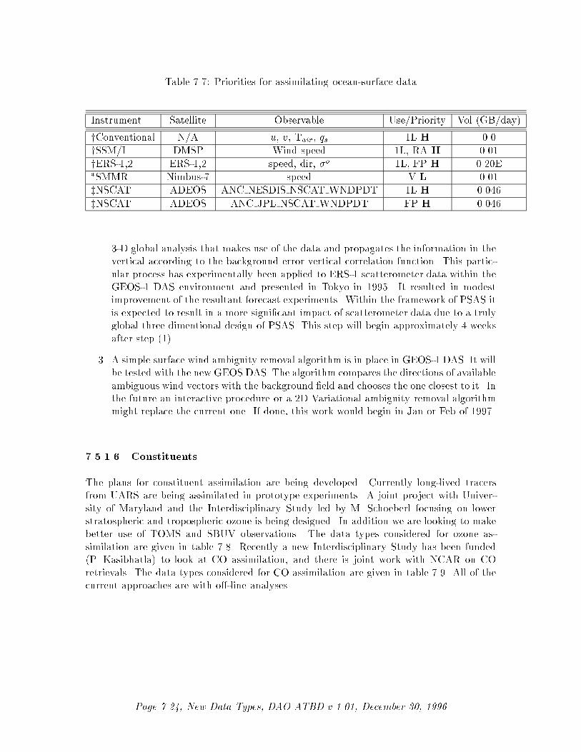
Table 7.7: Priorities for assimilating ocean-surface data
Instrument Satellite Observable Use/Priority Vol (GB/day)
yConventional N/A u, v, Tair, qs 1L H 0.0
ySSM/I DMSP Wind speed 1L, RA H 0.01
yERS-1,2 ERS-1,2 speed, dir, �o 1L, FP H 0.20E�SMMR Nimbus-7 speed V L 0.01
zNSCAT ADEOS ANC NESDIS NSCAT WNDPDT 1L H 0.046
zNSCAT ADEOS ANC JPL NSCAT WNDPDT FP H 0.046
3-D global analysis that makes use of the data and propagates the information in the
vertical according to the background error vertical correlation function. This partic-
ular process has experimentally been applied to ERS-1 scatterometer data within the
GEOS-1 DAS environment and presented in Tokyo in 1995. It resulted in modest
improvement of the resultant forecast experiments. Within the framework of PSAS it
is expected to result in a more signi�cant impact of scatterometer data due to a truly
global three dimentional design of PSAS. This step will begin approximately 4 weeks
after step (1).
3. A simple surface wind ambiguity removal algorithm is in place in GEOS-1 DAS. It will
be tested with the new GEOS DAS. The algorithm compares the directions of available
ambiguous wind vectors with the background �eld and chooses the one closest to it. In
the future an interactive procedure or a 2D Variational ambiguity removal algorithm
might replace the current one. If done, this work would begin in Jan or Feb of 1997.
7.5.1.6 Constituents
The plans for constituent assimilation are being developed. Currently long-lived tracers
from UARS are being assimilated in prototype experiments. A joint project with Univer-
sity of Maryland and the Interdisciplinary Study led by M. Schoeberl focusing on lower
stratospheric and tropospheric ozone is being designed. In addition we are looking to make
better use of TOMS and SBUV observations. The data types considered for ozone as-
similation are given in table 7.8. Recently a new Interdisciplinary Study has been funded
(P. Kasibhatla) to look at CO assimilation, and there is joint work with NCAR on CO
retrievals. The data types considered for CO assimilation are given in table 7.9. All of the
current approaches are with o�-line analyses.
Page 7.24, New Data Types, DAO ATBD v 1.01, December 30, 1996

Table 7.8: Priorities for assimilating ozone data
Instrument Satellite Observable Use/Priority Vol (GB/day)
yTOMS N7/Meteor/ADEOS total OA H 0.01
ySBUV N7/POES prof V (OA) H 0.001
yConven. N/A prof V H 0.0
ySAGE ERBS, etc. strat prof V H 0.0
yMLS UARS upper strat prof V H 0.02
yGOME ERS-2 total, prof V L ?
yTOVS POES (GLA) lower strat V L 0.2�CLAES UARS upper strat prof V L 0.02�HALOE UARS upper strat prof V L 0.02
zILAS ADEOS upper strat prof V L ?
zIMG ADEOS lower strat prof V L ?
Table 7.9: Priorities for assimilating CO data
Instrument Satellite Observable Use/Priority Vol (GB/day)
�MAPS Shuttle prof OA H 0.0
zMOPITT EOS AM prof OA H TBD
yConven. N/A prof V H 0.0
7.5.1.7 Wind pro�le
Currently, wind pro�le data used in GEOS are obtained from radiosondes and derived cloud
track winds. Several of the data types listed in table 7.10 appear to be strong candidates for
assimilation (e.g., water vapor winds similar to cloud track winds). Water vapor winds will
soon become available through the current operational data link. These new data types can
enhance the coverage of current wind pro�le data. However, because there is little heritage
for assimilating these data types, they are presently selected for validation. As resources
permit, some of these data types may eventually be assimilated.
7.5.1.8 Aerosols
Although consideration has been given to aerosol assimilation (M�enard, personal notes),
this topic has been given an overall low priority at present. Therefore, all data types listed
in table 7.11 were selected for validation.
7.5.2 Priorities grouped by satellite
This section categorizes high priority items by satellite. The priorities for the POES, UARS,
TRMM, ADEOS, and EOS AM-1 satellites are listed in tables 7.12-7.16, respectively.
Page 7.25, New Data Types, DAO ATBD v 1.01, December 30, 1996

Table 7.10: Priorities for assimilating wind pro�les
Instrument Satellite Observable Use/Priority Vol (GB/day)
yConventional N/A ANC NOAA RDSONDS OBS 1L H 0.01
yConventional N/A ACARS ANC NOAA ARCFT OBS 1L H 0.01
ycloud track GOES ANC NESDIS GOES WIND MOTION 1L H 0.008
yRADAR N/A trop/strat/mes VH ?
water vapor GOES/other trop V H ?�HRDI UARS strat/mes V L 0.003�WINDII UARS mes V L 0.03�MODE Shuttle V L ?
zSWIPE TBD
Table 7.11: Priorities for use of aerosol data
Instrument Satellite Observable Use/Priority Vol (GB/day)
ySAGE ERBS, etc. Strat V L 0.0
yTOMS Nimbus 7 Strat/Trop V L 0.01�CLAES UARS Strat V L 0.02�HALOE UARS Strat V L 0.02
zMISR EOS-AM properties V L ?
zILAS ADEOS Strat V L ?
Table 7.12: High-priority data types from POES satellite
Instrument Observable Use
yTOVS Temp. Prof/rad 1L
yTOVS H2O Prof/rad 1L
yTOVS Ts FP, RA
yAVHRR ANC NESDIS NDVI B, RA
Table 7.13: High-priority data types from UARS satellite
Instrument Observable Use
yMLS Strat T RA
yMLS Upper Trop/Strat H2O V
yMLS upper strat O3 V�CLAES Strat T V�HALOE Strat H2O V�HALOE upper strat prof O3 V
Page 7.26, New Data Types, DAO ATBD v 1.01, December 30, 1996

Table 7.14: High-priority data types from TRMM satellite
Instrument Observable Use
zTMI PR Prof (M69) FP
zTMI,PR PR Prof (M73) V
zPR PR Prof (M72) V
zCERES cloud (CER07) V
Table 7.15: High-priority data types from the ADEOS satellite
Instrument Observable Use
zNSCAT wind speed, dir, �o FP
yTOMS total O3 OA
7.5.3 Priorities grouped by use in GEOS
This section categorizes high priority items according to use in GEOS. Data types are
grouped as either used for �rst look, �nal platform (data types in addition to those used for
the �rst look), or reanalysis/pocket analysis (may include data types used in the �rst look
and �nal platform) in tables 7.17-7.19, respectively. Some of the high-risk data types (such
as land-surface data) have not been included here. Data types used for validation are not
listed here.
Page 7.27, New Data Types, DAO ATBD v 1.01, December 30, 1996

Table 7.16: High-priority data types from EOS AM1 satellite
Instrument Observable Use
zMODIS NDVI B, FP
zMODIS LAI, FPAR B, FP
zMODIS Evaptrans B, FP
zMODIS BidirRe B, FP
zMODIS Land type B, FP
zMODIS LS res B, FP
zMODIS Cloud V
zMODIS Ts V
zMODIS T,q Prof (MOD30) V
zMOPITT CO Prof OA
zCERES TOA, cloud (CER07) V
Table 7.17: High-priority data types for �rst look system
Instrument Platform Observable Volume
yConventional N/A ANC NOAA RDSONDS OBS 0.010
yTOVS, ATOVS POES (NESDIS) ANC NESDIS TOVS THKN RETS (T, q, radiance) 0.030
yConventional ship, buoy u, v, Tair , qs 0.0
ySSM/I DMSP ANC MSFC SSMI PRCP WATER 0.050
ySSM/I DMSP Wind speed 0.01
yERS-1 ERS-1 speed, dir 0.20E
zNSCAT ADEOS ANC NESDIS NSCAT WNDPDT 0.046
yConventional N/A ACARS ANC NOAA ARCFT OBS 0.01
ycloud track GOES ANC NESDIS GOES WIND MOTION 0.008
Table 7.18: High-priority data types for �nal platform.
Instrument Platform Observable Volume
ySSM/I DMSP Prec rate, surf 0.04
zTMI TRMM (M69) TMI PROF L2A-12 1.314S
zNSCAT ADEOS ANC JPL NSCAT WNDPDT 0.046
zMODIS EOS AM NDVI (MOD34 L3 10DY) 93.558GB/10day-S
zMODIS EOS AM LAI, FPAR (MOD15 L4 10DY) 1.502GB/10day-S
zMODIS EOS AM Evaptrans (MOD16 L3 10DY) 22.537GB/10day-S
zMODIS EOS AM (MOD09 BRDF L3 16DY) 108.16GB/16day-S
zMODIS EOS AM Land type (MOD12 L3 32DY) 0.417/32day-S
zMODIS EOS AM LS res (MOD41 L2) 23.652/day???
Page 7.28, New Data Types, DAO ATBD v 1.01, December 30, 1996

Table 7.19: High-priority data types for reanalysis and/or pocket analysis.
Instrument Platform Observable Volume
yMLS UARS Strat T 0.02
yTOVS POES (GLA) T, q 0.2
7.6 References
Adler, R., C. Kidd, M. Goodman, A. Ritchie, R. Schudalla, G. Petty, M. Morrissey, and S. Greene,1996: On the relation between ozone and potential vorticity, PIP-3 Intercomparison Results,PIP-3 Workshop, 18-20 November 1996, College Park, MD.
Andersson, E., Pailleux, J., Th�epaut, J. N., Eyre, J. R., McNally, A. P., Kelly, G. A., andP. Courtier, 1994: Use of cloud-cleared radiances in three/four-dimensional variational dataassimilation. Q. J. R. Meteorol. Soc., 120, 627-653.
Daley, R., 1995: Estimating the wind �eld from chemical constituent observations: Experimentswith a one-dimensional extended Kalman �lter. Mon. Wea. Rev., 123, 181-198.
Dee, D. P., 1995: On-line estimation of error covariance parameters for atmospheric data assimila-tion. Mon. Wea. Rev., 123, 1128-1145.
Dee, D. P., and A. Trenholme, 1996: DAO QC Strategy Document, DAO O�ce Note 96-15. DataAssimilation O�ce, Goddard Space Flight Center, Greenbelt, MD 20771. Available on-linefromhttp://dao.gsfc.nasa.gov/subpages/office-notes.html.
Dee, D., C. Redder and A. da Silva, 1996: O�-line tuning of forecast and observation error covari-ance parameters. DAO O�ce Note, in preparation. Data Assimilation O�ce, Goddard SpaceFlight Center, Greenbelt, MD 20771. This O�ce Note will be available on-line fromhttp://dao.gsfc.nasa.gov/subpages/office-notes.html.
Eyre, J. R., 1992: A bias correction scheme for simulated TOVS brightness temperatures. ECMWFTech. Memo 176.
Guo, J. and A. M. da Silva, 1995: Computational Aspects of Goddard's Physical-space Statis-tical Analysis System (PSAS). Preprints, Second UNAM-CRAY Supercomputing Conf. on
Numerical Simulations in the Environmental and Earth Sciences. Mexico City, Mexico, 6pp.
Hollingsworth, A. and P. L�onnberg, 1989: The veri�cation of objective analyses: diagnostics ofanalysis system performance, Meteorol. Atmos. Phys., 40, 3{27.
Joiner, J. and A. M. da Silva, 1996: E�cient methods to Assimilate Satellite Retrievals Basedon Information Content. DAO O�ce Note 96-06. Data Assimilation O�ce, Goddard SpaceFlight Center, Greenbelt, MD 20771. Available on-line fromhttp://dao.gsfc.nasa.gov/subpages/office-notes.html.
Koster, R. D., and M. J. Suarez, 1992: Modeling the land surface boundary in climate models asa composite of independent vegetation stands, J. Geophys. Res., 97, 2697-2715.
Krishnamurti, T. N., Xue, J., Bedi, H.S., K. Ingles, and D. Oosterhof, 1991: Physical initializationfor numerical weather prediction over the tropics. Tellus, 43AB, 53-81.
Ledvina, D. V., and J. Pfaendtner, 1995: Inclusion of Special Sensor Microwave/Imager (SSM/I)total precipitable water estimates into the GEOS-1 Data Assimilation System, Mon. Weath.
Rev., 123, 3003-3015.
Page 7.29, New Data Types, DAO ATBD v 1.01, December 30, 1996
M�enard, R., 1995: Middle atmosphere assimilation of UARS constituent data using Kalman �lter-ing: Preliminary results. International symposium on assimilation of observations in meteo-
rology and oceanography, Tokyo, Japan, 273-278.
M�enard, R., 1996: Consistent assimilation of retrieved data (CARD), private notes and manuscriptin preparation.
Molod, A., H. M. Helfand, and L. L. Takacs, 1995: The climatology of parameterized physicalprocesses in the GEOS-1 GCM and their impact on the GEOS-1 Data Assimilation System,J. Climate.
NASA/Goddard Space Flight Center, 1994; Science Data Plan for the EOS Data and Information
System covering EOSDIS Version 0 and Beyond, Document version 4, Ed. M. Schwaller andB. Krupp.
Riish�jgaard, L. P., 1996: On four-dimensional variational assimilation of ozone data in weatherprediction models. (accepted for publication in the Q. J. R. Meteorol. Soc.)
Rodgers, C. D., 1990: Characterization and error analysis of pro�les retrieved from remote soundingmeasurements. J. Geophys. Res., 95, 5587-5595.
Pfaendtner, J., S. Bloom, D. Lamich, M. Seablom, M. Sienkiewicz, J. Stobie, A. da Silva, 1995:Documentation of the Goddard Earth Observing System (GEOS) Data Assimilation System{Version 1. NASA Tech. Memo. No. 104606, Vol. 4, Goddard Space Flight Center, Greenbelt,MD 20771. Available on-line fromhttp://dao.gsfc.nasa.gov/subpages/tech-reports.html.
Schubert, S.D., R. B. Rood, and J. Pfaendtner, 1993: An assimilated data set for earth scienceapplications. Bul. Amer. Meteor. Soc., 74, 2331-2342.
Schubert, S., C.-K. Park, Chung-Yu Wu, W. Higgins, Y. Kondratyeva, A. Molod, L. Tkacs, M.Seablom, and R. Rood, 1995: A Multiyear Assimilation with the GEOS-1 System: Overviewand Results. NASA Tech. Memo. 104606, Vol. 6. Goddard Space Flight Center, Greenbelt,MD 20771. Available on-line fromhttp://dao.gsfc.nasa.gov/subpages/tech-reports.html.
Schubert, S. D., 1996: DAO's Quality Assessment Team: De�nition and Planing Document. DAOO�ce.. Data Assimilation O�ce, Goddard Space Flight Center, Greenbelt, MD 20771. In
preparation. This O�ce Note will be available fromhttp://dao.gsfc.nasa.gov/subpages/office-notes.html.
Schubert, S. D. and R. Rood, 1995: Proceedings of the Workshop on the GEOS-1 Five-YearAssimilation. NASA Tech. Memo. 104606, Vol. 7, Goddard Space Flight Center, Greenbelt,MD 20771. Available on-line fromhttp://dao.gsfc.nasa.gov/subpages/tech-reports.html.
Sellers, P. J., Y. Mintz, Y. C. Sud, and A. Dalcher, 1986: A simple boisphere model (SiB) for usewithin general circulation models, J. Atmos. Sci., 43, 505-531.
Sienkiewicz, M., 1996a: The GLA TOVS rapid algorithm forward radiance modules and Jacobianversion 1.0, DAO O�ce Note 96-08. Data Assimilation O�ce, Goddard Space Flight Center,Greenbelt, MD 20771. Available on-line fromhttp://dao.gsfc.nasa.gov/subpages/office-notes.html.
Sienkiewicz, M., 1996b: Evaluation of RTTOV and GLA TOVS forward model and Jacobian, DAOO�ce Note 96-20. Data Assimilation O�ce, Goddard Space Flight Center, Greenbelt, MD20771. Available on-line fromhttp://dao.gsfc.nasa.gov/subpages/office-notes.html.
Page 7.30, New Data Types, DAO ATBD v 1.01, December 30, 1996

da Silva, A. M., Pfaendtner, J., Guo, J., Sienkiewicz, M., and S. E. Cohn, 1995: Assessing thee�ects of data selection with DAO's Physical-space Statistical Analysis System. Internationalsymposium on assimilation of observations in meteorology and oceanography, Tokyo, Japan,273-278.
da Silva, A. and C. Redder, 1995: Documentation of the GEOS/DAS Observation Data Stream(ODS) Version 1.0. DAO O�ce Note 95-01. Data Assimilation O�ce, Goddard Space FlightCenter, Greenbelt, MD 20771. Available on-line fromhttp://dao.gsfc.nasa.gov/subpages/office-notes.html.
da Silva, A., and J. Guo, 1996: Documentation of the Physical-Space Statistical Analysis System(PSAS) Part I: The Conjugate Gradiant Solver version PSAS-1.00 DAO O�ce Note 96-02.Data Assimilation O�ce, Goddard Space Flight Center, Greenbelt, MD 20771. Availableon-line fromhttp://dao.gsfc.nasa.gov/subpages/office-notes.html.
da Silva, A. M., C. Redder, and D. P. Dee, 1996: Modeling retrieval error covariances for at-mospheric data assimilation. Presented at the Eighth Conference on Satellite Meteorology,
Atlanta, GA, 28 January{2 February, 1996. Available on-line asftp://dao.gsfc.nasa.gov/pub/papers/dasilva/atlanta96/tuning.ps.Z.
da Silva, A., Ekers, K., and A. Conaty, 1996b: Requirements for DAO's On-Line Monitoring System(DOLMS) version 1.00, DAO O�ce Note 96-14. Data Assimilation O�ce, Goddard SpaceFlight Center, Greenbelt, MD 20771. Available on-line fromhttp://dao.gsfc.nasa.gov/subpages/office-notes.html.
Stobie, J, 1996: Data Assimilation Computing and Mass Storage Requirements for 1998. DAO
O�ce Note 96-16. Data Assimilation O�ce, Goddard Space Flight Center, Greenbelt, MD20771. Available on-line fromhttp://dao.gsfc.nasa.gov/subpages/office-notes.html.
Sto�elen A., and D. Anderson, 1995: The ECMWF contribution to the characterisation, inter-pretation, calibration, and validation of ERS-1 scatterometer backscatter measurements andwinds, and their use in numerical weather prediction models, European Space Agency Contract
Report.
Susskind, J., Rosen�eld, J., and D. Reuter, 1983: An accurate radiative transfer model for use inthe direct physical inversion of HIRS and MSU temperature sounding data. J. Geophys. Res.88, 8550-8568.
Susskind, J., and J. Pfaendtner, 1989: Impact of iterative physical retrievals on NWP. Report onthe Joint ECMWF/EUETSAT Workshop on the Use of Satellite Data in operational weatherprediction: 1989-1993. Vol. 1, 245-270. T. Hollingsworth, Ed.
Susskind, J. 1993: Water vapor and temperature. Atlas of Satellite Observations Related to Global
Change, Edited by R. J. Gurney, J. L. Foster. and C. L. Parkinson. Cambridge UniversityPress, Cambridge England, 89-128.
Takacs, L.L., A. Molod, and T. Wang, 1994: Documentation of the Goddard Earth ObservingSystem (GEOS) General Circulation Model{Version 1. NASA Tech. Memo. No. 104606,Vol. 1, Goddard Space Flight Center, Greenbelt, MD 20771. Available on-line fromhttp://dao.gsfc.nasa.gov/subpages/tech-reports.html.
Page 7.31, New Data Types, DAO ATBD v 1.01, December 30, 1996

7.7 Acronyms
7.7.1 General acronyms
DAO Data Assimilation O�ce
GEOS Goddard Earth Observing System (The name of the DAO
data assimilation system)
GCM General Circulation Model
DAS Data Assimilation System
QC Quality Control
NWP Numerical Weather Prediction
CARD Consistent Assimilation of Retrieved Data
PSAS Physical-space Statistical Analysis System
NASA National Aeronautics and Space Administration
GSFC Goddard Space Flight Center
MTPE Mission to Planet Earth
EOS Earth Observing System
EOSDIS Earth Observing System Data and Information System
NOAA National Oceanic and Atmospheric Administration
NCEP National Centers for Environmental Prediction (formerly, NMC)
NMC National Meteorological Center
NESDIS National Environmental Satellite Data and Information Service
ECMWF European Center for Medium-range Weather Forecasts
UKMO United Kingdom Meteorological O�ce
7.7.2 Instruments
ADEOS Advanced Earth Observting Satellite (Mid-late 1996)
AIRS Atmospheric Infrared Sounder (EOS PM)
AMSU A-B Advanced Microwave Sounding Unit (POES, EOS PM)
AVHRR Advanced Very High-Resolution Radiometer
ASTER Advanced Spaceborne Thermal Emission and Re ection
Radiometer (EOS AM)
ATOVS Advanced TOVS; HIRS3/AMSU (POES)
CERES Clouds and Earth's Radiation Energy System (TRMM, EOS AM)
CLAES Cryogenic Limb Array Etalon Spectrometer (UARS)
DMSP Defense Meteorological Satellite Program (currently operational)
EOS AM1 Earth Observting Satellite AM (June 98 launch)
EPS EUMETSAT (European Meteorology Satellite) Polar System
ERBE Earth Radiation Budget Experiment (ERBS)
ERBS Earth Radiation Budget Satellite
ERS-1,2 European Remote Sensing Satellite (Scatterometer,
6 channel, IR-Visible radiometer)
Page 7.32, New Data Types, DAO ATBD v 1.01, December 30, 1996

GOES Geostationary Observational Environmental Satellite
(Imager and 18 channel visible and infrared sounder,
currently operational)
GOME Global Ozone Monitoring Experiment (ERS-2)
GPS Global Positioning System
HALOE Halogen Occultation Experiment (UARS)
HIRS2/3 High-Resolution InfraRed Sounder (POES)
HRDI High Resolution Doppler Imager
IASI Infrared Atmospheric Sounding Interferometer (EPS)
ILAS Improved Limb Atmospheric Spectrometer (ADEOS)
IMG Interferometric Monitor for Greenhouse Gases (ADEOS)
ISCCP International Satellite Cloud Climatology Project (several
IR and visible instruments aboard di�erent satellite)
LIMS Limb Infrared Monitor of the Stratosphere (Nimbus 7)
MAPS Measurement of Atmospheric Pollution from Satellites
MHS Microwave Humidity Sounder (EOS-PM)
MLS Microwave Limb Sounder (UARS)
MODIS Moderate-Resolution Imaging Spectrometer (EOS AM)
MSU Microwave Sounding Unit
MOPITT Measurement of Pollution in the Troposphere (EOS AM)
NSCAT NASA Scatterometer (ADEOS)
POES Polar Orbiting Environmental Satellite (Currently Operational)
PR Precipitation Radar (TRMM)
SBUV Satellite Backscatter Ultraviolet radiometer (Nimbus 7, POES)
SAGE Stratospheric Aerosol and Gas Experiment (ERBS)
SMMR Scanning Multispectral Microwave Radiometer (?)
SSM/I Special Sensor Microwave/Imager (DMSP)
SSM/T Special Sensor Microwave (Temperature sounder, DMSP)
SSM/T2 Special Sensor Microwave (Water vapor sounder) (DMSP)
SSU Stratospheric Sounding Unit (POES)
TMI TRMM Microwave Imager (TRMM)
TOMS Total Ozone Mapping Spectrometer (ADEOS, Meteor,
Earth Probe, Nimbus 7)
TOVS TIROS Operational Vertical Sounder; HIRS2/MSU/SSU (POES)
TRMM Tropical Rainfall Measuring Mission (summer '97 launch)
UARS Upper Atmospheric Research Satellite (some instruments in operation)
WINDII Wind Imaging Interferometer (UARS)
Page 7.33, New Data Types, DAO ATBD v 1.01, December 30, 1996

Chapter 8
Quality Assessment/Validation ofthe GEOS Data AssimilationSystem
Contents
8.1 Validation for Earth-science Data Assimilation . . . . . . . . . 8.1
8.2 Overview of GEOS-2 Quality Assessment/Validation . . . . . . 8.4
8.2.1 System Validation . . . . . . . . . . . . . . . . . . . . . . . . . . . 8.4
8.2.2 Scienti�c Evaluation . . . . . . . . . . . . . . . . . . . . . . . . . . 8.5
8.2.3 Monitoring . . . . . . . . . . . . . . . . . . . . . . . . . . . . . . . 8.5
8.2.4 Infrastructure . . . . . . . . . . . . . . . . . . . . . . . . . . . . . . 8.6
8.3 GEOS-2 Validation Process . . . . . . . . . . . . . . . . . . . . . 8.7
8.3.1 The GEOS-1 Baseline . . . . . . . . . . . . . . . . . . . . . . . . . 8.7
8.3.2 Distillation of the GEOS-1 Baseline . . . . . . . . . . . . . . . . . 8.13
8.3.3 GEOS-2 Validation . . . . . . . . . . . . . . . . . . . . . . . . . . . 8.14
8.3.4 Absolute Validation . . . . . . . . . . . . . . . . . . . . . . . . . . 8.16
8.4 New Approaches to Validation . . . . . . . . . . . . . . . . . . . 8.18
8.5 GEOS-2 Validation Tasks . . . . . . . . . . . . . . . . . . . . . . . 8.20
8.6 References . . . . . . . . . . . . . . . . . . . . . . . . . . . . . . . . 8.21
8.7 Acronyms . . . . . . . . . . . . . . . . . . . . . . . . . . . . . . . . 8.26
8.7.1 General acronyms . . . . . . . . . . . . . . . . . . . . . . . . . . . 8.26
8.7.2 Instruments . . . . . . . . . . . . . . . . . . . . . . . . . . . . . . . 8.26
8.1 Validation for Earth-science Data Assimilation
Since the inception of the DAO validation of system performance and improvement has
been an open question. In the early reports of the DAO Science Advisory Panel, questions
were raised about how to validate in ways other than forecast skill. The DAO has always
worked from the premise that short and medium range forecast skill is not the absolute
Page 8.1, Validation, DAO ATBD v 1.01, December 30, 1996

measure of analysis quality. In fact, it is possible to improve forecast skill at the expense
of analysis accuracy. This situation arises because there are compensating errors in the
model-analysis-data system. Furthermore, many of the problems of interest to customers of
the DAO are so far removed from weather forecasting that the weather forecast is insensitive
to their representation. Therefore, more general methods of validation must be developed.
If the assimilation system is focused at generalized applications then the number of
possible problems to provide metrics to measure improvement becomes very large. Often
con icts develop because e�orts to improve performance in one area degrade performance
in another area. The temptation to �x a problem with an ad hoc speci�cation of a system
parameter is high. Inevitably �xes haunt future development, because �xes, almost by
de�nition, are short circuiting some feedback loop that is not well understood.
The DAO has grappled with the validation problem from the beginning. We maintain
an internal group focused on scienti�c applications of GEOS data sets in order to assure
that basic climate processes are evaluated. We continually seek and organize independent
validation data sets (see http://dao.gsfc.nasa.gov/ for the current archive). We maintain
a series of collaborations within GSFC to evaluate problems of atmospheric chemistry and
climate parameters. We maintain a collaboration with NCEP to intercompare NCEP and
DAO products. We have built a community of several hundred scientists who have looked at
the GEOS data sets with varying degrees of scrutiny. This section details the current status
of the DAO validation e�ort. More information can be found in Schubert et al. (1996).
One of the major goals of the GEOS-1 project (Chapter 4) was to develop a suite
of problems to serve as baseline metrics to evaluate future performance. The number
of problems identi�ed from GEOS-1 is too large for all of them to be treated as equal
metrics. Many are related to each other. Some are clearly beyond the near-term ability of
any assimilation system. There are resource issues as con icts development, for instance,
between the need to improve ozone transport and the need to improve the surface energy
balance.
Therefore, the DAO is faced with the problem of de�ning priorities to the di�erent
problems. These priorities are prescribed based on the science priorities of the MTPE
(see Section 2.6), customer base, speci�cally focused funding, projected ability to impact a
particular problem, performance relative to other available products, and initiatives in the
broad science community. With so many di�erent pulls on the process, validation is made
even more di�cult. There can be focus and improvement on one aspect of the system, and
inattention to other aspects. In order to damp some of this volatility we have tried to focus
on two broad disciplines which are at the basis of many aspects of Earth science:
� global hydrological and energy cycles, including interaction between the atmosphere
ocean and land surfaces and storage in the soil
� transport processes in the atmosphere in order to calculate quantitatively dynamic
variability of tropospheric and stratospheric trace constituents
One conclusion of our e�orts has been the realization that assessment of the quality of the
data assimilation system extends beyond traditional validation. With multi-year assimilated
data sets and parallel experiments with identical models techniques are being developed
that bridge the gap between traditional space and time averaged climate diagnostics and
Page 8.2, Validation, DAO ATBD v 1.01, December 30, 1996

process-oriented modeling. We are discovering fundamental research questions that must be
answered in order to develop soundly based validation criteria. This chapter will focus on
the quality assessment plans for GEOS systems. At the time of this writing the validation for
GEOS-2 is in progress and much is being learned about system integration and validation.
GEOS-2 validation is, therefore, the focus of the chapter. Status of the GEOS-2 validation
can be found at
http://zymurgy.gsfc.nasa.gov/lamich/geos2.0/closure/CM/status.html
In an attempt to manage the quality assessment process we have identi�ed three major
components:
1. System validation
2. Scienti�c evaluation
3. Monitoring
These major components will be described below.
Page 8.3, Validation, DAO ATBD v 1.01, December 30, 1996

8.2 Overview of GEOS-2 Quality Assessment/Validation
The validation of data assimilation systems has traditionally focused on measuring the
improvement in the accuracy of the forecast of the state variables of the atmosphere. This
re ects the development of data assimilation as a method for improving numerical weather
forecasts. Therefore, forecast skill is, culturally, the current fundamental measure of the
quality of the assimilated product.
Over the past 15 years the scienti�c community has come to realize that assimilated
atmospheric data provide a unique resource for studying the dynamics of the atmosphere.
In fact, the analyses being routinely generated by the operational numerical weather pre-
diction (NWP) community have become indispensable tools for studying a wide array of at-
mospheric science problems. Traditionally, the NWP products su�er from inhomogeneities
resulting from system changes (e.g., Trenberth and Olson 1988; Arpe 1990), which have
made them inappropriate for many studies focused on longer term weather and climate
variations. The NWP products also have, historically, not included many of the diagnostic
quantities (e.g., precipitation, heat rates, radiative uxes, etc.) needed for studying climate
processes. This likely re ects a lack of con�dence in the quality of these quantities, the
secondary importance these have received in the validation of NWP analyses, as well as the
substantial expense of their generation and storage.
Recently, to address the problem of spurious signals from system changes, a number of
centers have generated re-analyses of historical observations (Schubert et al. 1993; Gibson
et al. 1994; Kalnay et al. 1996). For the DAO e�ort, the re-analysis (employing GEOS-
1, Chapter 4) provided a unique opportunity to both produce a benchmark for further
development and to provide a timely product to the science community. While the GEOS-1
DAS has a strong NWP heritage, the primary goal of this e�ort was to seek feedback from
a wide as possible range of users to help guide the development of future versions of the
GEOS system (Schubert and Rood 1995, TM Volume 7). One of the key lessons learned
from this e�ort is that validation of assimilation products is in its infancy - there is no
simple measure of quality that is appropriate for the entire array of potential applications.
The quality assessment e�ort within the DAO (Schubert et al. 1996) is attempting
to address this broader role of validation by employing an integrated approach closely
coupled with the development and production process, involving system validation, scienti�c
evaluation, and monitoring.
8.2.1 System Validation
System validation is the process by which major modi�cations to the system are evaluated
and judged suitable for incorporation into the next production system. This e�ort is perhaps
the most demanding in terms of coordination with other activities. In particular, it must
determine how to best coordinate with, complement, and take advantage of the ongoing
validation activities inherent in the development process. In addition, it must bring to bear
the results of the relevant scienti�c investigations, new veri�cation data, and the diagnostic
tools which are best suited for evaluating the system modi�cations at hand. It must also
tackle the daunting task of quantifying the quality of the assimilated products for climate
and other Earth Science applications. Without this link to representative Earth- science
Page 8.4, Validation, DAO ATBD v 1.01, December 30, 1996

problems the validation can lose relevance.
The process of system validation is an evolving one; we have yet to learn how to best
ensure that the validation process is directly linked to the requirements of our customers.
These requirements (Chapter 9) may be con icting and as such the validation e�ort must
be given guidance on priorities which may be based on other than scienti�c justi�cations.
There are, for example, special production requirements on accuracy and timeliness imposed
by the EOS instrument teams.
8.2.2 Scienti�c Evaluation
The centerpiece of the DAO quality assessment e�ort is the scienti�c evaluation of the assim-
ilated products. This requires multi-year data sets to assess the ability of the assimilation
system to faithfully reproduce the mean climate, its variations and the associated physical
processes. While a considerable amount of work is done within the DAO and other Goddard
Laboratories (e.g., codes 913 and 916) , the broad range of potential applications necessitate
that much of the assessment of the quality of the GEOS DAS products be carried out by
outside investigators. To ensure this takes place it is imperative that the DAO periodically
produce and make available useful long term assimilated data sets to the general science
community.
The in-house scienti�c assessment has been divided into four areas of research consisting
of
IH1: climate variability and sensitivity
IH2: stratospheric meteorology and transport
IH3: regional climate, weather and the hydrological cycle
IH4: tropospheric chemistry.
There is signi�cant in-house experience in these four areas, and a history of applica-
tions de�ne the necessary improvements needed to address speci�c scienti�c projects. The
usefulness of the assimilated data for addressing science issues in each of these areas, gener-
ally depends on the internal (physical and dynamical) consistency of the assimilated data,
which in turn depends on the veracity of the physical processes represented in the geophysi-
cal model and their consistency with the observations. Furthermore, the degree to which the
assimilated data track nature depends on the availability and quality of observations, and
the ability of the analysis scheme to extract and optimally combine the relevant information
from the observations and model-generated �rst guess �elds.
8.2.3 Monitoring
The real-time monitoring of on-going data assimilation experiments is crucial to a successful
production e�ort. The general goal of monitoring is to ensure that any errors in the process-
ing are detected (and possibly corrected) at an early stage before substantial resources are
wasted. This includes the monitoring of both the input observations and output assimilated
Page 8.5, Validation, DAO ATBD v 1.01, December 30, 1996

data and ancillary information (such as quality control information) which characterize the
quality of the assimilated product.
A requirements document for monitoring the output from an assimilation (da Silva et al.,
1996) provides the framework for the initial implementation of the DAO On-line Monitoring
System (DOLMS). The requirements are tailored to the speci�c modes of operation of
the GEOS DAS involving the �rst-look analysis, the �nal platform analysis, multi-year re-
analyses, and system validation experiments (see Section 2.6.3). As outlined in the DOLMS
document, the monitoring system for the �rst-look analysis must provide on- line access
to recent analyses, forecasts, quality control information and selected climate diagnostics.
The monitoring system for the �nal platform analysis will be similar but with the addition
of statistics for monitoring new (both active and passive) data types. For multi-year re-
analyses the monitoring system will focus on time series at key locations or regional averages
and on a comprehensive collection of climate diagnostics. If forecasts are issued these will
be monitored in a way similar to the �rst look system. The monitoring system for system
validation will focus on monthly time series and climate diagnostics with the additional
capability to simultaneously depict the performance of the new system compared to the
control system.
DOLMS can be reviewed at
http://dao.gsfc.nasa.gov/monitoring
DOLMS capabilities are being continually upgraded. The DOLMS page and some of
the experiments represented there are volatile and contain errors that are being addressed
in validation projects. Therefore none of the results on the DOLMS page should be used
for scienti�c applications without �rst contacting the DAO.
8.2.4 Infrastructure
In order to support the validation e�ort a substantial infrastructure is needed. Beaudoin
and Schubert (1996) describe the visualization and user interface that plays a vital role in
managing and integrating validation and development resources. These resources consist of
veri�cation data, subsets of assimilated data, visualization and other scienti�c tools, and
documentation.
Page 8.6, Validation, DAO ATBD v 1.01, December 30, 1996

8.3 GEOS-2 Validation Process
8.3.1 The GEOS-1 Baseline
The process of evolving the data assimilation system from one version to the next is volatile,
often driven by discoveries made during the process. During development, modi�cations
are built upon an existing frozen, validated system. The experience from the frozen system
de�nes the baseline on which to validate the next system. Documentation of both known
de�ciencies and validated features of the frozen system is needed.
The GEOS-1 experiment (Chapter 4) provided the baseline for improvement of GEOS-
2. In this section we review the GEOS-1 system. The validated features (successes) and
identi�ed shortcomings of the GEOS-1 system are summarized here. Schubert and Rood
(1995, TM Volume 7) provide a more detailed exposition of both successes and failures of
GEOS-1. De�ciencies that have been discovered since the publication of Schubert and Rood
are also included here.
8.3.1.1 Validated Features (Successes) of the GEOS-1 DAS
The relative validation described in Section 8.3.3.1 involves the comparison of features in the
system being considered with those from the latest frozen or control system. This requires
a documented list of validated features which will be updated at each system validation
step. Since the GEOS-2 validation is the �rst major system validation exercise, we present
below (in lieu of o�cially validated features for GEOS-1) a list of features that have been
documented as being well captured by the DAS.
8.3.1.1.1 Low Frequency Variability. The primary strength of the GEOS-1 assim-
ilation system lies in its ability to capture many of the key patterns of climate variations
associated with El Nino and La Nina events, monsoons, droughts and other low frequency
variations. These consist of the following:
� The global signature of low frequency variations in the atmospheric moisture �eld
compare favorably with SSM/I data. (Chen et al. 1995).
� The tropical zonal winds and pressure �elds have realistic variations associated with
the Madden-Julian Oscillation and westerly wind bursts. (Lau et al. 1995) The large
scale tropical divergent wind �eld captures the evolution of the Madden-Julian Oscil-
lation (Schubert et al. 1995, Mo and Higgins 1996).
� The large cloud forcing anomaly in the central equatorial Paci�c associated with
1986/87 El Nino compares favorably with ERBE data (Chen and Bates 1995). The
tropical Paci�c outgoing longwave radiation (OLR) anomalies associated with the
1987/88 El Nino/La Nina event compare favorably with OLR observations (Schubert
et al. 1995). The monsoon precipitation anomalies associated with the 1987/88 El
Nino/La Nina event are consistent with the OLR observations (Schubert et al. 1995).
Page 8.7, Validation, DAO ATBD v 1.01, December 30, 1996

� The reduced precipitation during the 1988 (June) drought and the much enhanced
precipitation during the 1993 (July) wet conditions over the United States compare
favorably with station observations (Schubert et al. 1995).
� GEOS-1 captures the seasonal placement of upper tropospheric moisture patterns
quite well (Salathe and Chesters 1995)
8.3.1.1.2 Short Term Variability. A number of shorter term uctuations are well
represented in the assimilation. These are primarily associated with uctuations in the
zonal wind and/or the boundary layer winds and surface stresses. These consist of:
� The GEOS-1 equatorial winds appear to successfully capture the sub-daily atmo-
spheric tidal variations (Salstein and Rosen 1995).
� GEOS-1 winds compared with length of day measurements suggest that the momen-
tum variations are well captured for periods as short as 8-9 days. Comparisons be-
tween NCEP and GEOS-1 re-analyses shows coherence on all time scales longer than
3 days, which is shorter (better) than has been typically obtained from operational
analyses. This suggests the re-analyses are in closer agreement than operational series
have been in the past for this quantity (Salstein and Rosen 1995).
� The horizontal winds, convective cloud mass ux, detrainment, and planetary bound-
ary layer depth are of su�cient quality to be used with signi�cant success as input
to tropospheric chemistry transport models for Freon-11, Rn-222, and CO. Middle
latitude synoptic variability is well captured; however, interhemispheric gradients are
not well simulated. Convective transport suggests that the cloud mass uxes are of
the right magnitude (Allen et al. 1995; Pickering et al. 1995).
� GEOS-1 wind stress provides good estimates of ocean transport through the Florida
Straits. The GEOS wind stress generally provides improvements over the operational
ECMWF results, but tends to overestimate amplitudes beyond about 10 days (Great-
batch and da Silva 1995).
� Variations in the low level winds over the Great Plains are quite realistic despite the
lack of observations going into the GEOS-1 DAS below 850 hPa (Helfand et al. 1995).
8.3.1.1.3 Climate Mean. The following climate mean quantities are generally consis-
tent with available verifying observations, and/or are consistent or better than found in
other analyses:
� The climate mean and seasonal evolution of the tropospheric zonal wind appears to
be well captured (Schubert et al. 1995).
� The clear sky longwave ux and albedo are in good agreement with ERBE measure-
ments. See, however, below comment concerning a cancellation of errors (Charlock
and Rose 1995; Chen and Bates 1995; Wu et al. 1995; Arking 1995).
Page 8.8, Validation, DAO ATBD v 1.01, December 30, 1996

� The general patterns of tropical convection and their seasonal evolution are consis-
tent with available observations, but details of local maxima and amplitudes are not
(Robertson et al. 1995).
� The wind stress �elds have been employed to force an ocean model in the North Paci�c
with some success in producing the sub-polar circulation (Rienecker 1995).
8.3.1.1.4 Stratosphere The stratospheric version of GEOS-1 DAS has the following
validated features:
� Forecasts from the GEOS system have been used with general success in planning and
directing ights of the high-altitude NASA ER-2 aircraft to potential vorticity, and
hence chemical, targets in middle and high latitudes (Newman et al. 1995).
� Lagrangian tracking techniques have been successful in mapping tracer structures that
are much �ner than the resolution of the assimilating model. Tracking of the Pinatubo
eruption cloud with GEOS winds has been more successful than similar experiments
with NCEP winds.
� GEOS winds have been successfully used to model ozone chemistry and transport for
integrations longer than one year. Prior experiments that did not use the IAU were
not useful for more than a three month integration. Synoptic and planetary-scale
variability are well simulated (Douglass et al. 1995, Douglass et al. 1996).
� The rotated pole model e�ectively eliminates spurious noise that was noted at the
pole in earlier versions of the GEOS analysis. The location of the computational pole
at low latitudes does not appear to cause a problem; this is likely because the Coriolis
term is small (T.-C. Chen, Takacs, Min, unpublished results).
� The tropical quasi-biennial wind oscillation is present in the analyses. Though details
of the quasi-biennial oscillation are not well represented, the variability is far better
than has ever been achieved in GCM calculations.
8.3.1.2 De�ciencies of the GEOS-1 DAS
It is from the identi�cation and confrontation of our weaknesses that future strengths are
built.
The primary de�ciencies in the GEOS-1 DAS products are tied to errors in the water
vapor and cloud �elds. This is not unique to GEOS-1 as all analyses continue to have
problems with these parameters. The humidity bias, in particular, has been linked to a
number of problems with the GEOS-1 assimilation system. One of the most disturbing
de�ciencies is an apparent feedback between the analysis increments and the model �rst
guess �elds which generates spurious tropical cloudiness and precipitation intensities which
are unrealistic (particularly during boreal summer) and, in fact, in some cases less accurate
than that simulated by the model (Molod et al. 1996, and see section 4.3.1.2). Another is
a strong sensitivity of the assimilated climate to moisture observations (Park et al. 1996)
which leads to arti�cial climate signals tied to inhomogeneities in the input observations.
Page 8.9, Validation, DAO ATBD v 1.01, December 30, 1996

Another place where the data insertion reduces the quality obtained by the model simu-
lation is in the representation of the surface energy balance. In particular, the GEOS-1 DAS
has excessively cold surface temperatures over land during winter (Schubert et al. 1995).
In this case, the insertion of observed moisture and temperature pro�les lead to a reduction
in large-scale cloudiness generated by the model, which in turn produces excessive radiative
cooling to space. These instances where the assimilation of data degrades the performance
of the model in simulation mode require the highest attention.
In general, the di�erences between the behavior of the system in simulation and assim-
ilation mode have presented unforeseen di�culties with both tuning and overall validation
e�orts. Not surprisingly, tuning (or cancellation of errors in general) can lead to mislead-
ing conclusions on the quality of the system. An example, is the excessive water vapor
in the upper tropospheric and stratospheric water vapor (Starr et al. 1995; Charlock and
Rose 1995). This occurs despite a very good match between the GEOS-1 DAS and ERBE
clear sky outgoing long wave radiation (OLR). This rather misleading result appears to be
the result of a cancellation of errors (Takacs, personal communication) with excessive upper
level moisture and too little moisture in the lower troposphere (Molod et al. 1996). The
close match between the ERBE and DAS clear sky OLR in GEOS-1 is also suspect in view
of the missing contribution from trace gases in the current radiation code (Suarez, personal
communication).
Below we summarize the known de�ciencies in the GEOS-1 DAS products.
D1: Moisture and clouds
� A much too wet upper troposphere (300 hPa) over the Paci�c Ocean compared with
available observations and other analyses (Starr et al. 1995; Charlock and Rose 1995).
� The horizontal moisture gradients between very moist and very dry regions of the
upper troposphere are too weak (Salathe and Chesters 1995).
� The tropics and subtropics over the oceans are too dry compared with the vertically
integrated moisture from SSM/I (Molod et al. 1996; Ledvina and Pfaendtner 1995).
� Longwave and shortwave cloud radiative forcing are overestimated over regions of deep
convection in the intertropical convergence zone (ITCZ) especially during Northern
summer (Molod et al. 1996; Wu et al. 1995; Charlock and Rose 1995; Chen and
Bates 1995; Ledvina and Hou 1996; Arking 1995).
� Middle-latitude longwave and shortwave cloud radiative forcing are weaker than ERBE
especially over the storm tracks of both hemispheres (Molod et al. 1996; Chen and
Bates 1995). The vertical distribution of diabatic heating and vertical heat transport
may also be too shallow in these regions (especially the North Atlantic, Straus and
Paolino 1995).
� High clouds in the tropics are excessive. Middle and low clouds in extratropics are
de�cient (Joseph and Geller 1995).
� Low level coastal stratiform clouds are underestimated (Wu et al. 1995).
Page 8.10, Validation, DAO ATBD v 1.01, December 30, 1996

� Cloud mass ux associated with June squall line over Kansas and Oklahoma is too
shallow (Pickering et al. 1995)
� Cloud mass ux does not entrain and detrain mass over a deep enough layer. There-
fore, the boundary layer and upper troposphere are linked too strongly. Conse-
quently the middle troposphere is too isolated from convective processes. (Pickering
et al. 1995; Allen et al. 1995)
� De�cient tropospheric interhemispheric exchange (Allen et al. 1995)
D2: Precipitation, evaporation and near surface �elds
� Precipitation over eastern Paci�c ITCZ is underestimated (Ledvina and Pfaendtner,
1995).
� Summertime precipitation over eastern North America is overestimated (Schubert et
al. 1995; Higgins et al. 1996; Arpe and Stendel 1995).
� Springtime evaporation over central and eastern United States is too large (Schubert
and Chang 1996; Higgins et al. 1996).
� The amplitude of the diurnal cycle of the precipitation over the southeast US is too
large with little evidence of a nocturnal maximum over the Great Plains (Higgins et
al. 1996; Min and Schubert 1996a, b).
� The amplitude of the annual cycle of tropical precipitation/OLR is too large (Kon-
dragunta and Gruber 1996; Yang and Schubert 1996).
� Interannual variability in precipitation is too weak (Kondragunta and Gruber 1996;
Yang and Schubert 1996).
� Wintertime precipitation is too low over the Northern Rockies and along the southern
coast of the United States (Arpe and Stendel 1995).
� The gap in precipitation between the western Ghats and the Bay of Bengal is missing
(Arpe and Stendel 1995).
� Rain over continental Europe and northern Asia in July is excessive. Rain over the
Mediterranean during January is weak (Arpe and Stendel 1995).
� Precipitation over Caribbean and Gulf of Mexico during summer is excessive (Adler
et al. 1996).
� Days with small rain amounts are too frequent. Days with no rain are too few. Days
with intense rain amounts are underestimated (Wood et al. 1995; Higgins et al. 1996;
Min and Schubert 1996a,b)
� The 1988 drought over the United States extends too long into the summer with
warmer and drier conditions than were observed in July (Schubert et al. 1995).
� The near surface temperature is too cold over the northern United States and Canada
during winter (Schubert et al. 1995).
Page 8.11, Validation, DAO ATBD v 1.01, December 30, 1996

� The implied oceanic heat transport based on the net heat ux into the ocean is
unrealistically large (da Silva and White 1995).
� Subtropical deserts are less re ective than in ERBE. The diurnal cycle of out- going
longwave radiation over land shows signi�cant phase shifts with respect to ERBE
(Joseph and Geller 1995).
� Subtropical/middle latitude (e.g. in region of Kuroshio current) wind stress is too
weak (Rienecker 1995; Rienecker et al. 1996).
D3: Wind, temperature and pressure �elds
� The Hadley cell is too weak during Northern winter (Arpe and Stendel 1995; Hou,
personal communication; Schubert et al. 1995; DeWeaver and Nigam 1996).
� Zonal mean sea level pressure and zonal wind are biased (Arpe and Stendel 1995;
Takacs and Suarez 1996).
� Transport (heat, momentum, and moisture) by NH transient waves is too strong and
by stationary waves too weak (Min et al. 1996; Takacs and Suarez 1996).
� Baroclinic energy conversions in synoptic and smaller scales are weak (Straus and
Paolino 1996).
� The northward component of the summertime low level wind over the southern Great
Plains and Gulf Coast appears to be underestimated (Higgins et al. 1996).
� Various quantities including the temperature, wind and sea level pressure show evi-
dence of noise near the poles (Takacs and Suarez 1996).
� Small scale noise in stratosphere tropics is excessive (Douglass et al. 1996)
� \barrier" between tropics and middle latitudes is too weak in lower stratosphere (Dou-
glass et al. 1996).
� Stratospheric tropical upward motion is too strong. Polar winter descent is too weak
(Newman et al. 1995; Douglass et al. 1995; 1996)
� There is a warm bias at the stratospheric wintertime pole for the most extreme cold
events. (Newman et al. 1995)
� Tropical Kelvin waves are not well represented.
� Five-day tropospheric forecast skill is not competitive (Atlas et al. 1996)
� Tropical stratospheric forecasts are poor (Newman et al. 1995).
Page 8.12, Validation, DAO ATBD v 1.01, December 30, 1996
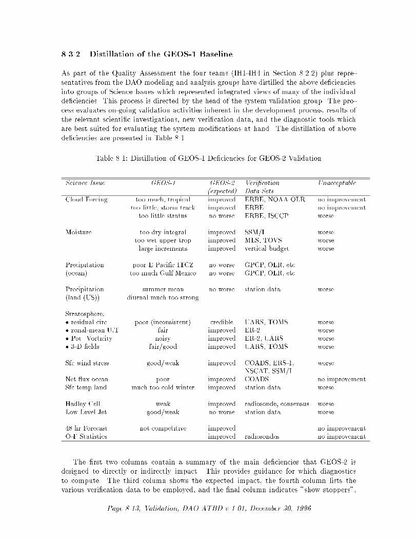
8.3.2 Distillation of the GEOS-1 Baseline
As part of the Quality Assessment the four teams (IH1-IH4 in Section 8.2.2) plus repre-
sentatives from the DAO modeling and analysis groups have distilled the above de�ciencies
into groups of Science Issues which represented integrated views of many of the individual
de�ciencies. This process is directed by the head of the system validation group. The pro-
cess evaluates on-going validation activities inherent in the development process, results of
the relevant scienti�c investigations, new veri�cation data, and the diagnostic tools which
are best suited for evaluating the system modi�cations at hand. The distillation of above
de�ciencies are presented in Table 8.1.
Table 8.1: Distillation of GEOS-1 De�ciencies for GEOS-2 Validation
Science Issue GEOS-1 GEOS-2 Veri�cation Unacceptable
(expected) Data Sets
Cloud Forcing too much, tropical improved ERBE, NOAA OLR no improvementtoo little, storm track improved ERBE no improvement
too little stratus no worse ERBE, ISCCP worse
Moisture too dry integral improved SSM/I worsetoo wet upper trop improved MLS, TOVS worselarge increments improved vertical budget worse
Precipitation poor E Paci�c ITCZ no worse GPCP, OLR, etc(ocean) too much Gulf Mexico no worse GPCP, OLR, etc
Precipitation summer mean no worse station data worse(land (US)) diurnal much too strong
Stratosphere:� residual circ poor (inconsistent) credible UARS, TOMS worse� zonal-mean U,T fair improved ER-2 worse� Pot. Vorticity noisy improved ER-2, UARS worse� 3-D �elds fair/good improved UARS, TOMS worse
Sfc wind stress good/weak improved COADS, ERS-1, worseNSCAT, SSM/I
Net ux ocean poor improved COADS no improvementSfc temp land much too cold winter improved station data worse
Hadley Cell weak improved radiosonde, consensus worseLow Level Jet good/weak no worse station data worse
48 hr Forecast not competitive improved no improvementO-F Statistics improved radiosondes no improvement
The �rst two columns contain a summary of the main de�ciencies that GEOS-2 is
designed to directly or indirectly impact. This provides guidance for which diagnostics
to compute. The third column shows the expected impact, the fourth column lists the
various veri�cation data to be employed, and the �nal column indicates "show stoppers",
Page 8.13, Validation, DAO ATBD v 1.01, December 30, 1996

i.e. a result that would bring the validation to a halt and require immediate attention of
the validation committee. The teams are monitoring the performance of these parameters
as GEOS-2 experiments are run. New capabilities of GEOS-2 and GEOS-3, such as soil
moisture, will be validated in component models during the development stage, but ultimate
validation will depend upon the results from applications.
8.3.3 GEOS-2 Validation
Prior to the actual implementation of the validation process, a detailed validation plan is
written (Schubert et al. 1996). The plan ensures that all aspects of validation are carried
out and �nally, to decide (based on the results of the validation diagnostics), whether or not
the system modi�cations have lead to an acceptable new production version of the DAS.
System validation is constrained by time and resources to a limited set of experiments.
This complicates the determination of climate variability and sensitivity characteristics
which require comparisons between di�erent years. As such, the validation outlined here
can only be preliminary, trying to catch egregious errors and anticipate performance when
longer data sets are available. Re-analyses carried out with validated systems become an
integral part of the overall scienti�c evaluation. Results from long assimilations with GEOS-
2 will form the basis for further development and provide input for the system validation
of future systems.
Hence, a major early decision is what experiments to run for validation. The choice is not
easy. Many of the de�ciencies identi�ed by users are for speci�c time periods. While they
might represent general process de�ciencies, often the user only has quantitative information
on a small number of case studies. Also, some of the validation data sets are only available
for a particular time. It is impossible to produce multi-year data sets in a timely fashion
for system validation.
The validation steps carried out as part of the development process must also be recon-
ciled with the �nal system validation. This module testing of individual system components
must be carried out in a controlled fashion and documented for evaluation by the full val-
idation committee. The decision as to what constitutes a major modi�cation (or group of
modi�cations) and requires system integration and a full system validation step is as yet
unclear, though it is certainly clear that the GEOS-2 validation process is hampered by an
abundance of modi�cations that are all coming on-line simultaneously. (Currently a process
is being de�ned to use the Scienti�c Steering Board of the DAO. The Scienti�c Steering
Board is an internal group, reporting to the Head, of DAO, comprised of individuals who
represent all key aspects of the GEOS system and MTPE mission requirements.)
For the current validation of GEOS-2.0, we are generating assimilations from three
periods for comparisons to the control (GEOS, STRAT, the con�guration of GEOS-1 that
fully resolves the stratosphere); these assimilations will begin in mid May of 1987 and 1988
and mid December of 1991. Each run will consist of one and one half months of assimilation
with a one half month period of spin-up time. Numerous repeats are performed as problems
are identi�ed and corrected. A one year GEOS-2.0 model simulation will be carried out in
parallel to help assess the causes of de�ciencies found in the assimilation.
System validation of GEOS-2 will pursue two strategies: relative validation and absolute
Page 8.14, Validation, DAO ATBD v 1.01, December 30, 1996

validation. Relative validation compares the behavior of the current (candidate) system
with that of a previous system (control). The control's performance has been baselined.
Where the control system has had previously acceptable (i.e validated) performance, it is
reasonable to require the candidate system to perform at a similar level.
Absolute validation evaluates the products of a candidate system by comparing them
to products obtained from independent data. An absolute validation criterion is satis�ed
when the candidate system value agrees with the independent validation standard within the
uncertainties inherent in both the candidate and validation standard values. The uncertain-
ties (i.e. error bars) in the validation data will be complicated combinations of instrument,
sampling and even modeling errors. Thus, while absolute validation is generally the most
desirable approach to follow in order to address scienti�c issues, it is also a more challenging
approach to perform correctly.
Note: the summary in Table 8.1 contains issues pertaining to both validation strategies.
In the following we expand on the relative and absolute validation approaches to be used
for the GEOS-2 system validation.
8.3.3.1 Relative Validation
There are a number of objective measures available for comparing the behavior of GEOS-
2 against a control system. In relative validation short-term forecasting plays a substantial
role. This addresses some of the lessons learned from the GEOS-1 project listed in Chap-
ter 4. The following list is a descriptive summary of those that will be used for the system
validation of GEOS-2.
8.3.3.1.1 O-F statistics. How well does the candidate system forecast future data?
O-F statistics are the mean variance, for pre-de�ned regions and selected data types at
various levels of the atmosphere, of di�erences of observations from 6-hour model forecast
�elds. Although the variance of O-F should not be zero (since there are observational
errors), the general guiding principle is that an improved system should show decreases in
O-F variances.
8.3.3.1.2 QC statistics. QC (quality control) statistics are an accounting of the num-
ber of data which fail the quality control checks within a particular system. The tropics,
mid-latitudes and polar regions will be examined separately. A large number of observations
failing the QC generally indicates a drift in the assimilation system away from observations.
This, along with growing O-F's, is usually a sign of defect in an assimilation system.
8.3.3.1.3 A-F spectra, time means. A-F spectra are the Fourier spectra of analysis
minus forecast (analysis increments) around latitude circles. Power at high wave numbers
is generally indicative of noise in the analysis. Does the candidate system have reduced A-F
spectra at high wave numbers?
Time means of analysis increments can be revealing of possible biases in the assimilation
system (especially in the GCM component). A non-zero time mean A-F indicates that the
Page 8.15, Validation, DAO ATBD v 1.01, December 30, 1996

analysis (and, by inference, data) is constantly �ghting changes introduced by the GCM
integration since a previous analysis.
8.3.3.1.4 O-A statistics O-A statistics (observation minus analysis residuals) are a
measure of howwell an analysis extracts information from data (Hollingsworth and L�onneberg 1989).
Here O-A statistic refers to the covariance between analyses and some speci�c observation
type (e.g. rawinsonde heights); in particular, this diagnostic focuses on the (extrapolated)
intercept of the O-A covariance at zero distance. An intercept of zero or a negative value
indicates that the analysis is extracting the maximum available information from that ob-
servation type.
8.3.3.1.5 Forecast skill - Anomaly Correlations Anomaly correlations will be gen-
erated from the suite of forecasts made from initial conditions taken from the assimilation
runs. Our interest is on the short-term (1-3, up to 5 days) anomaly correlation behavior,
as that re ects to a greater degree on the nature of the assimilation system's handling of
data and to a lesser degree on strictly performance of the forecast model. The higher the
anomaly correlation, the better the result.
In Chapter 5 are numerous examples of relative validation. They show a measure of
new system performance relative to old system performance. O-F statistics are shown in
Figure 5.27 to show that in both January and July the system with the incremental analysis
update draws forecasts to the background state with greater accuracy. Figures 5.2 through
5.4 show spectra of analysis increments which reveal that the Physical-space Statistical
Analysis System reduces the spurious noise at high wavenumbers relative to the old optimal
interpolation.
8.3.4 Absolute Validation
Absolute validation is the foundation of system validation. It is the part of the validation
activity that is most directly tied to speci�c science and/or operational objectives. It forms
the basis for judging whether the GEOS system meets the various customer requirements
(see Chapter 9) and thus measures the success of the overall GEOS DAS development e�ort.
Absolute validation requires that measures of product quality be formulated to re ect the
impact on speci�c science and/or operational requirements. It is only within such a context
that meaningful measures of \accuracy" and pre-de�ned criteria for designating a particular
product feature to be of acceptable quality can be made. This, in turn, requires that
uncertainties in the estimates of the DAS product and the veri�cation data be considered.
Since absolute validation requires independent data sets, the DAO continually seeks and
organizes independent validation data sets (see http://dao.gsfc.nasa.gov/ for the current
archive). While there are a few consensus data sets accepted by the community as standards,
for many primary parameters (e. g. precipitation) there is not general consensus. In most
of these more uncertain parameters there is wide spread in the range of the independent
validation data sets.
It is worth noting that the most widely accepted standard for accuracy of temperature
and wind measurements are rawinsondes. Therefore, rawinsonde data are at the very basis
Page 8.16, Validation, DAO ATBD v 1.01, December 30, 1996

of absolute validation. It is often biases and root mean square (rms) di�erences with raw-
insondes that are the �rst line of validation. An absolute standard is also at the very basis
of bias correction techniques (See Chapter 9).
The fourth column in Table 8.1 lists some of the key independent veri�cation data that
will be used for the GEOS-2 absolute validation. These range from the relatively accurate
rawinsonde reports of winds to the much less certain cloud information from the ISCCP
data. How these data are used also impacts the accuracy of the comparison. For example,
the use of N2O transport calculations to assess the quality of the GEOS winds must take into
account not only the accuracy of the UARS N2O data but also the uncertainties inherent
in the o�-line transport calculations.
Requirements to provide ancillary data for instrument retrievals are sometimes the eas-
iest to deal with in terms of formulating speci�c measures of quality. For example, the
CERES instrument team requires moisture and temperature pro�les with speci�c (rms)
accuracies and bias tolerances. The GEOS-2 products will be compared with rawinsonde
reports of these quantities where available, and with other satellite observations of these
quantities to determine whether the GEOS-2 products meets these requirements.
Science requirements are more di�cult to formulate and can often only be addressed
indirectly. For example, the outgoing longwave radiation (OLR) must meet certain bias and
rms tolerances (compared with ERBE data) which are linked to the accuracy of the upper
level moisture �eld, the cloud distribution and cloud optical properties. These tolerances
must be set to allow climate sensitivity studies of sea-surface temperature and upper level
moisture as well as to provide accurate surface energy balances at the ocean surface to
produce reasonable implied ocean heat transports.
Those items in Table 8.1 having speci�c entries in the column labeled "Veri�cation" will
be the subjects of absolute validation activities for GEOS-2. The detailed absolute valida-
tion plans for each of these, including the speci�c links to science/customer requirements
are currently being formulated. The end result of the absolute validation activity is a list
of validated features of the GEOS-2 DAS that will be updated with each new validation
activity.
Page 8.17, Validation, DAO ATBD v 1.01, December 30, 1996

8.4 New Approaches to Validation
The pursuit of generalized data assimilation opens up a whole range of new questions. Many
of these questions have never been addressed, and are fundamental research issues.
For instance, the production of re-analyses removed the spurious signals from multi-
year data sets caused by analysis systems that were continually changing to improve weather
forecasts. The re-analyses have been successful in providing information about interseasonal
and interannual variability. New questions are now raised about the variability of the input
data stream. Concerns about the variability of the input data stream include
ID1: a new type of data becomes available
ID2: a di�erent instrument makes the same type of measurement
ID3: The same instrument degrades in time
ID4: a di�erent data handling process is applied to data provided by outside sources
Clearly, for instance, given the tremendous shortcomings in the cloud and precipitation
�elds, data from a MTPE platform such as the Tropical Rainfall Measurement Mission
(TRMM) will have a dramatic change on data set quality. This will leave a spurious signal
in the long-term data set. There are many open questions in how to best address the impact
of the changing input data stream.
But there are many more subtle problems with the input data stream than the avail-
ability of a completely new data type. One of the most important lessons learned from the
re- analysis projects is the impact of quality control decisions. Park et al. (1996) show,
for example, that Indian monsoon rainfall uctuations are at least in part associated with
uctuations in the number of radiosonde moisture observations that were ingested in the
GEOS-1 DAS. The impact of observations, in particular, the extent to which they constrain
the assimilation, and the extent to which they are optimally utilized by the assimilation
system are key validation issues that are just beginning to be addressed.
Sienkiewicz and Pfaendtner (1996) showed, for example, that di�erences in the initial
conditions for an assimilation can be traced for several weeks, depending on the data dis-
tribution, on the model formulation, and on the parameter that is being studied. One
consequence of this research is to de�ne how much overlap is required and what is the
impact on long-term variability from piecing together short data sets to create long data
sets?
Other new validation techniques focus on physical and dynamical consistency, one of the
most important expectations of assimilated data sets. The lack of consistency between the
state variables and parameterized diagnostic or forcing quantities substantially reduces the
value of the DAS products for many applications. The lack of consistency typical manifests
itself as a mean arti�cial source/sink term in budget equations that, in current assimilated
data, are comparable in magnitude to the physical forcing. In this respect data assimilation
is itself an important validation exercise, since the mismatch between the observations and
�rst guess �elds can form the basis for judging the quality of the system.
Page 8.18, Validation, DAO ATBD v 1.01, December 30, 1996

Schubert and Chang (1996) embraced this idea to address the physical and dynami-
cal consistency of the U.S. hydrological cycle within the GEOS-DAS. A methodology was
developed (Restricted Statistical Correction or RSC) that allows output from DAS runs
to be used directly to infer the sources of the model errors. The RSC approach, in fact,
suggests more general validation criteria that measure the extent to which the observations
systematically (and thus improperly) in uence the assimilated climate.
The consistency question brings attention to model parameterizations and how they
impact estimates of poorly constrained parameters. Chang and Schubert (unpublished)
have conducted sensitivity studies where a subtle change to the convective parameterization
leads to uncertainties in the assimilated tropical wind �eld of up to 30the climate variance.
Finally, understanding the climate generated by a data assimilation requires that we
understand the climate of the geophysical model employed in the assimilation system. Such
long simulations employing the same model used in the assimilation have previously been
unavailable. Mismatches between the simulate and assimilate climates can provide new
insights into the de�ciencies of the assimilation system (Molod et al. 1996). Such simulations
can also be used to look more carefully at the constraints imposed on the climate system.
The extent to which these constraints are not satis�ed in climate simulations should help
to address model de�ciencies and help quantify science requirements (e.g., Johnson 1996,
MIT 1996).
Page 8.19, Validation, DAO ATBD v 1.01, December 30, 1996

8.5 GEOS-2 Validation Tasks
In consideration of the constraints on time and computing resources, the validation runs
will be limited to two boreal summer and one boreal winter assimilations. The tentative
schedule is outlined below:
Development and integration of the proposed GEOS-2.0 system will be completed on
a pre-speci�ed date (PD). At this time the new system will be set to run three 2 1/2
assimilations; two will begin in mid May 1987, 1988 while the other will begin in mid
December 1991. These three years have been chosen for a number of reasons, though
ultimately the choice was based on the availability of some of the key veri�cation data sets
(particularly ERBE data for 1987, 1988 and UARS data for 1991/92). The comparison of
1987 and 1988 allows an assessment of interannual variability associated with ENSO.
A control employing GEOS-1.2 has already produced results for these time periods.
Two business days (2D) will be allotted for preparation of a restart �le for each assimilation
and for the preparation time needed to set-up each assimilation run (e.g. scripts and
directories). Thus, beginning on PD + 2D the three assimilations will begin running in
parallel (on separate computers) in support of the validation e�ort.
Each run will undergo a one half month assimilation check to verify the model and the
analysis are operating as expected. Extensive use will be made of the DOLMS to ensure
there are no obvious errors. When running an assimilation it takes about one half of a
month for spin-up time so this check is based on the results of the spin-up. During the
assimilation runs, �ve-day forecasts will automatically be generated every 6th day (limited
to June/July 1988 and Jan/Feb 1992). This is not expected to add to the amount of time to
complete the assimilation since both the assimilation and forecasts can run simultaneously.
Based on the current resources provided, it should take about four days to run one half
month of assimilation for GEOS 2.0 and two days to run a thorough check of the spin-up.
Sixteen days is the expected time to run the remainder of the two and one half month
assimilations. Allowing an additional week for contingencies, this phase of the work should
be completed on PD + 2D + 27D.
Responsibilities for each area of validation (see Table 8.1) are assigned in advance as
part of the initial meetings of the Validation Panel. After the two and one half months of
assimilation for the three periods and the suite of forecasts are complete, epvaluation of the
diagnostics will commence. A complete package of all results will be completed in 15 days
(15D).
The Validation Panel will be assembled and given the results of the validation tests.
Based on the results, each panel member will decide how the system performed in each of
the areas shown in Table 8.1 It is expected that the system will meet most of the expectations
and have none of the show stoppers listed in Table 8.1. A written evaluation by each panel
member must be completed and submitted to the chair of the Validation Panel within seven
days followed by a �nal meeting of the Validation Panel to vote on whether the proposed
system is acceptable. A �nal summary report documenting the decision of the Panel will
be made within one week.
Page 8.20, Validation, DAO ATBD v 1.01, December 30, 1996
8.6 References
Adler, R., C. Kidd, M. Goodman, A. Ritchie, R. Schudalla, G. Petty, M. Morrissey and
S. Greene: PIP-3 Intercomparison Results, Oct 1996, prepared for PIP-3 Workshop
18-20 November 1996, College Park, MD.
Allen, D., R. Hudson, R. Rood, and A. Thompson, 1995: F-11 and Rn-222 calculations
using a 3-D CTM and assimilated data, proceedings of the Workshop on the GEOS-1
Five- Year Assimilation, NASA Tech. Memo. No. 104606, Volume 7, Goddard Space
Flight Center, Greenbelt, MD 20771.
Arkin, A., 1995: Shortwave Radiation Absorption in Clear and Cloudy Atmospheres.
Proceedings of the Workshop on the GEOS-1 Five-Year Assimilation, NASA Tech.
Memo. No. 104606, Volume 7, Goddard Space Flight Center, Greenbelt, MD 20771.
Arpe, K. 1990: Impact of changes in the ECMWF analysis-forecasting scheme on the
systematic error of the model, Ten years of medium-range weather forecasting, Volume
1, 4-8 September 1989, June 1990, ECMWF, Shin�eld Park, Reading RG2 9AX, U.K.
Arpe, K. and M. Stendel 1995: Comparison of GEOS-1 data with analysis and short-
range forecast data from ECMWF and other estimates of truth. Proceedings of the
Workshop on the GEOS-1 Five-Year Assimilation, NASA Tech. Memo. No. 104606,
Volume 7, Goddard Space Flight Center, Greenbelt, MD 20771.
Atlas, R., R. N. Ho�man, E. Brin, S. Bloom and P. M. Woiceshyn 1996: The impact of
ERS-1 scatterometer data on GEOS and NCEP model forecasts, 11th Conference on
Numerical Weather Prediction, 99-101, August 19-23, 1996, Norfolk, Va.
Beaudoin, P. and S. Schubert, 1996: Visualization and user interface: requirements docu-
mentation, to appear as DAO O�ce Note.
Charlock, T. P. and F. G. Rose, 1995: Comparison of Pre-CERES, Satellite-Based Calcu-
lations of Atmospheric Longwave Radiation Budget with GEOS-1. Proceedings of the
Workshop on the GEOS-1 Five-Year Assimilation, NASA Tech. Memo. No. 104606,
Volume 7, Goddard Space Flight Center, Greenbelt, MD 20771.
Chen, T.-C., J. Pfaendtner, J.-M. Chen, and C. K. Wikle, 1995: Variability of the Global
Precipitable Water with a Time-Scale of 90-150 Days. Proceedings of the Workshop
on the GEOS-1 Five-Year Assimilation, NASA Tech. Memo. No. 104606, volume 7,
Goddard Space Flight Center, Greenbelt, MD 20771.
Chen, M. and J. R. Bates, 1995: Cloud Radiative Forcing: GEOS-1 Assimilation Versus
ERBE Observation, proceedings of the Workshop on the GEOS-1 Five-Year Assim-
ilation, NASA Tech. Memo. No. 104606, volume 7, Goddard Space Flight Center,
Greenbelt, MD 20771.
DeWeaver, E. and S. Nigam, 1996: Di�erences between NASA/GEOS assimilated and
ECMWF analyzed divergent circulatations: causes and dynamical implications for El
Nino wintertime anomalies, submitted to J. Atmos. Sci.
Page 8.21, Validation, DAO ATBD v 1.01, December 30, 1996

Douglass, A. R., C. J. Weaver, R. B. Rood, and L. Coy, 1995: A Three Dimensional
Simulation of the Ozone Annual Cycle Using winds from a Data Assimilation System,
proceedings of the Workshop on the GEOS-1 Five-Year Assimilation, NASA Tech.
Memo. No. 104606, volume 7, Goddard Space Flight Center, Greenbelt, MD 20771.
Douglass, A. R., C. J. Weaver, R. B. Rood, and L. Coy, 1996: A three-dimensional sim-
ulation of the ozone annual cycle using winds from a data assimilation system, J.
Geophys. Res., 101, 1463-1474.
Gibson, J. K., P. Kallberg, A. Nomura and S. Uppala, 1994: The ECMWF re-analysis
(ERA) project-plans and current status, Tenth International Conference on Interactive
Information and Processing Systems for Meteorology, Oceanography and Hydrology,
American Meteorological Society, Nashville, Tennessee.
Greatbatch, R. J. and A. M. da Silva, 1995: Using GEOS-1 Wind Stress to Model the
Variation of Transport Through the STraits of Florida. Proceedings of the Workshop
on the GEOS-1 Five-Year Assimilation, NASA Tech. Memo. No. 104606, volume 7,
Goddard Space Flight Center, Greenbelt, MD 20771.
Helfand, H. M., S. D. Schubert and C.-Y. Wu, 1995: Characteristics of the Simulated and
Assimilated Great Plains Low Level Jet. Proceedings of the Workshop on the GEOS-1
Five-Year Assimilation, NASA Tech. Memo. No. 104606, volume 7, Goddard Space
Flight Center, Greenbelt, MD 20771.
Higgins, R. W., K. C. Mo and S. D. Schubert, 1996: The moisture budget of the cen-
tral United States in spring as evaluated in the NMC/NCAR and the NASA/DAO
reanalyses, Mon. Wea. Rev.,124, 939-963.
Hollingsworth, A. and P. L�onnberg, 1989: The veri�cation of objective analyses: diagnos-
tics of analysis system performance, Meteorol. Atmos. Phys., 40, 3-27.
Johnson, D. R. 1996: On the `General Coldness of Climate Models' and the second law:
implications for modeling the Earth System, to be submitted.
Joseph, R. R., and M. A. Geller, 1995: Comparison of the Diabatic Fields in the GEOS
DAS with those in the Atmosphere. Proceedings of the Workshop on the GEOS-1
Five- Year Assimilation, NASA Tech. Memo. No. 104606, volume 7, Goddard Space
Flight Center, Greenbelt, MD 20771.
Kalnay, E., M. Kanamitsu, R. Kistler, W. Collins, D. Deaven, J. Derber, L. Gandin,
S. Sara, G. White, J. Woollen, Y. Zhu, M. Chelliah, W. Ebisuzaki, W. Higgins,
J. Janowiak, K. C. Mo, C. Ropelewski, J. Wang, A Leetma, R. Renolds, R Jenne,
1995: The NMC/NCAR Reanalysis Project, Bulletin of the American Meteorological
Society, 77, 437 - 471.
Kondragunta, C. R. and A. Gruber, 1996: Intercomparison of spatial and temporal vari-
ability of precipitation products, Advances in Space Research, to appear.
Lau, K.-M., P. J. Sheu , S. Schubert, D. Ledvina, and H. Weng, 1995: Evolution of Large
Scale Circulation During TOGA-COARE: Model Intercomparison and Basic Features,
Proceedings of the Workshop on the GEOS-1 Five-Year Assimilation, NASA Tech.
Memo. No. 104606, volume 7, Goddard Space Flight Center, Greenbelt, MD 20771.
Page 8.22, Validation, DAO ATBD v 1.01, December 30, 1996

Ledvina, D. V. and J. Pfaendtner, 1995: Inclusion of Special Microwave/Imager (SSM/I)
total precipitable water estimates into the GEOS-1 data assimilation system, Mon.
Wea. Rev., 123, 3003-3015.
Ledvina, D. V. and A. Hou, 1996: Data impact studies using the GEOS-1 DAS during
TOGA COARE: Inclusion of SSM/I total precipitable water and surface wind esti-
mates, WMO TOGA 95, in press.
MIT Climate Sensitivity Workshop, 1996: Estimating climate variability and sensitivity
from satellite observations-Summary Report from the MIT Climate Sensitivity Work-
shop, April 21-22, 1996, Cambridge, MA
Min W. and S. Schubert, 1996a: A summary of precipitation statistics over the United
States. DAO O�ce Note 96-17. Data Assimilation O�ce, Goddard Space Flight
Center, Greenbelt, MD 20771. Available on-line from
http://dao.gsfc.nasa.gov/subpages/office-notes.html.
Min W. and S. Schubert, 1996b: The climate signal in regional moisture uxes: A com-
parison of three global assimilation products, J. Climate, submitted.
Min W., S. Schubert and C.-K. Park, 1996: Am intercomparison of assimilated and simu-
lated atmospheric variance/covariance statistics, NASA Tech. Memo. No. 104606, in
preparation, Goddard Space Flight Center, Greenbelt, MD 20771.
Mo, K. C. and R. W. Higgins, 1996: Large Scale Atmospheric Water Vapor Transport as
Evaluated from the NCEP/NCAR and NASA/DAO Reanalyses. J. Climate, in press.
Molod, A., H. M. Helfand, and L. L. Takacs, 1996: The climate of the GEOS-1 GCM and
its impact on the GEOS-1 data assimilation system, J. Climate, 9, 764-785.
Newman, P., L. Lait, M. Schoeberl, M. Seablom, L. Coy, D. Lamich, R. Rood, R. Stimp e
and K. R. Chan, 1995: The use of GEOS-1 data for the Airborne Southern Hemi-
sphere Ozone Experiment (ASHOE) and the Measurements for Assessing the E�ects of
Stratospheric Aircraft (MAESA) mission, proceedings of the Workshop on the GEOS-
1 Five-Year Assimilation, NASA Tech. Memo. No. 104606, volume 7, Goddard Space
Flight Center, Greenbelt, MD 20771.
Park, C.-K., S.-D. Schubert, D. J. Lamich, and Y. Kondratyeva, 1996: Monsoon Rainfall
in the GEOS-1 Assimilation: Sensitivity to Input Data. DAO O�ce Note 96-24. Data
Assimilation O�ce, Goddard Space Flight Center, Greenbelt, MD 20771. Available
on-line from
http://dao.gsfc.nasa.gov/subpages/office-notes.html.
Pickering, K. E. , W.-K. Tao, Y. Wang, J. R. Scala, A. M. Thompson, D. P. McNamara,
S.- J. Lin, A. M. Molod, and R. B. Rood, 1995: Transport Investigations Using the
GEOS-1 Convective Fluxes, proceedings of the Workshop on the GEOS-1 Five-Year
Assimilation, NASA Tech. Memo. No. 104606, volume 7, Goddard Space Flight
Center, Greenbelt, MD 20771.
Rienecker, M., 1995: A comparison of surface wind products over the North Paci�c Ocean,
proceedings of the Workshop on the GEOS-1 Five-Year Assimilation, NASA Tech.
Memo. No. 104606, volume 7, Goddard Space Flight Center, Greenbelt, MD 20771.
Page 8.23, Validation, DAO ATBD v 1.01, December 30, 1996

Rienecker, M. M., R. Atlas, S. D. Schubert, and C. A. Scholz, 1995: A comparison of
surface wind products over the North Paci�c Ocean, J. Geophys. Res.-Oceans, 101,
1011- 1023.
Robertson, F., W. Lapenta, D. Samuelson, J. Srikishen, and E. McCaul, 1995: Divergent
Circulations and Deep Convective Processess in the GEOS-1 Assimilated Fields as
Compared to Remotely Sensed Data. Proceedings of the Workshop on the GEOS-1
Five-Year Assimilation, NASA Tech. Memo. No. 104606, volume 7, Goddard Space
Flight Center, Greenbelt, MD 20771.
Salathe, E. P. Jr. and D. Chesters, 1995: Evaluation of Upper-Tropospheric Moisture
in the GEOS Assimilation Using TOVS Radiance Observations. Proceedings of the
Workshop on the GEOS-1 Five-Year Assimilation, NASA Tech. Memo. No. 104606,
volume 7, Goddard Space Flight Center, Greenbelt, MD 20771.
Salstein, D. A. and R. Rosen, 1995: Global Momentum and Energy Diagnostics from
the GEOS-1 Assimilation. Proceedings of the Workshop on the GEOS-1 Five-Year
Assimilation, NASA Tech. Memo. No. 104606, volume 7, Goddard Space Flight
Center, Greenbelt, MD 20771.
Schubert, S. D., R. B. Rood, J. W. Pfaendtner, 1993: An assimilated data set for earth
science applications, Bull. Amer. Meteor. Soc., 74, 2331-2342.
Schubert, S., C.-K, Park, C.-Y. Wu, W. Higgins, Y. Kondratyeva, A. Molod, L. Takacs,
M. Seablom. R. Rood, 1995: A multiyear assimilation with the GEOS-1 system:
overview and results, NASA Tech. Memo. No. 104606, volume 6, Goddard Space
Flight Center, Greenbelt, MD 20771.
Schubert, S. D. and R. B. Rood, 1995: Proceedings of the Workshop on the GEOS-1 �ve-
year assimilation, NASA Tech. Memo. No. 104606, volume 7, Goddard Space Flight
Center, Greenbelt, MD 20771.
Schubert, S. D. and Y. Chang, 1996: An objective method for inferring sources of model
error, Mon. Wea. Rev., 124, 325-340.
Schubert, S. D., S. C. Bloom, K. Ekers, 1996: Validation Plan for Version 2.0 of the
Goddard Earth Observing System (GEOS) Data Assimilation System, O�ce Note
xx-96 (to appear), Data Assimilation O�ce.
Sienkiewicz, M. E., and J. Pfaendtner, 1996: Assimilation Variability in the GEOS-1 DAS,
to appear Mon. Wea. Rev.
da Silva, A., and G. White, 1995: A Comparison of Surface Marine Fluxes from GEOS-
1/DAS and NMC Reanalyses. Proceedings of the Workshop on the GEOS-1 Five-
Year Assimilation, NASA Tech. Memo. No. 104606, volume 7, Goddard Space Flight
Center, Greenbelt, MD 20771.
da Silva, A., K. Ekers, and A. Conaty, 1996: Requirements for DAO's On-Line Monitoring
System (DOLMS) Version 1.00, DAO O�ce Note 96-13. Data Assimilation O�ce,
Goddard Space Flight Center, Greenbelt, MD 20771.
Page 8.24, Validation, DAO ATBD v 1.01, December 30, 1996

Starr, D., B. Diehl, A. Lare and B. Soden, 1995: Upper Tropospheric Humidity in the
5- Year GEOS Assimilation, proceedings of the Workshop on the GEOS-1 Five-Year
Assimilation, NASA Tech. Memo. No. 104606, volume 7, Goddard Space Flight
Center, Greenbelt, MD 20771.
Straus, D. M. and D. Paolino, 1995: Diabatic Heating in the NASA DAO Re-analyses:
Interactions with dynamics, proceedings of the Workshop on the GEOS-1 Five-Year
Assimilation, NASA Tech. Memo. No. 104606, volume 7, Goddard Space Flight
Center, Greenbelt, MD 20771.
Straus, D. M. and D. Paolino, 1996: Diagnosis of the mid-latitude baroclinic regime in the
NASA DAO reanalyses and ECMWF operational analyses, Center for Ocean-Land-
Atmosphere Studies, Report No. 25, March 1996.
Takacs, L. L., and, M. J. Suarez, 1996: Evaluation of the climate of the GEOS-1 GCM:
Dynamical processes, NASA Tech. Memo. No. 104606, volume 10, Goddard Space
Flight Center, Greenbelt, MD 20771.
Trenberth, K. E., and J. G. Olson, 1988: ECMWF global analyses 1979-1986: Circulation
statistics and data evaluation, NCAR Technical Note, NCAR/TN-300+STR, Boulder,
CO.
Wood, E. F., T. Stevens, and R. Koster, 1995: Analysis of GEOS-1 Rainfall Data for
Hydrological Modeling, proceedings of the Workshop on the GEOS-1 Five-Year As-
similation, NASA Tech. Memo. No. 104606, volume 7, Goddard Space Flight Center,
Greenbelt, MD 20771.
Wu, M.-L. C., K. M. Lau, P. Beaudoin and W. Smith, 1995: Studies of the radiation budget
at the top of the atmosphere and surface energy budget from the 5-Year Assimilation
with the Goddard Earth Observation System, proceedings of the Workshop on the
GEOS-1 Five-Year Assimilation, NASA Tech. Memo. No. 104606, volume 7, Goddard
Space Flight Center, Greenbelt, MD 20771.
Yang, R. and S. Schubert, 1996: Variability of tropical precipitation as inferred from a
nine-year GEOS-1 Assimilation, J. Climate, to be submitted.
Page 8.25, Validation, DAO ATBD v 1.01, December 30, 1996

8.7 Acronyms
8.7.1 General acronyms
DAO Data Assimilation O�ce
GEOS Goddard Earth Observing System (The name of the DAO
data assimilation system)
GCM General Circulation Model
DAS Data Assimilation System
QC Quality Control
NWP Numerical Weather Prediction
CARD Consistent Assimilation of Retrieved Data
PSAS Physical-space Statistical Analysis System
NASA National Aeronautics and Space Administration
GSFC Goddard Space Flight Center
MTPE Mission to Planet Earth
EOS Earth Observing System
EOSDIS Earth Observing System Data and Information System
NOAA National Oceanic and Atmospheric Administration
NCEP National Centers for Environmental Prediction (formerly, NMC)
NMC National Meteorological Center
NESDIS National Environmental Satellite Data and Information Service
ECMWF European Center for Medium-range Weather Forecasts
UKMO United Kingdom Meteorological O�ce
8.7.2 Instruments
ADEOS Advanced Earth Observting Satellite (Mid-late 1996)
AIRS Atmospheric Infrared Sounder (EOS PM)
AMSU A-B Advanced Microwave Sounding Unit (POES, EOS PM)
AVHRR Advanced Very High-Resolution Radiometer
ASTER Advanced Spaceborne Thermal Emission and Re ection
Radiometer (EOS AM)
ATOVS Advanced TOVS; HIRS3/AMSU (POES)
CERES Clouds and Earth's Radiation Energy System (TRMM, EOS AM)
CLAES Cryogenic Limb Array Etalon Spectrometer (UARS)
DMSP Defense Meteorological Satellite Program (currently operational)
EOS AM1 Earth Observting Satellite AM (June 98 launch)
EPS EUMETSAT (European Meteorology Satellite) Polar System
ERBE Earth Radiation Budget Experiment (ERBS)
ERBS Earth Radiation Budget Satellite
ERS-1,2 European Remote Sensing Satellite (Scatterometer,
6 channel, IR-Visible radiometer)
Page 8.26, Validation, DAO ATBD v 1.01, December 30, 1996

GOES Geostationary Observational Environmental Satellite
(Imager and 18 channel visible and infrared sounder,
currently operational)
GOME Global Ozone Monitoring Experiment (ERS-2)
GPS Global Positioning System
HALOE Halogen Occultation Experiment (UARS)
HIRS2/3 High-Resolution InfraRed Sounder (POES)
HRDI High Resolution Doppler Imager
IASI Infrared Atmospheric Sounding Interferometer (EPS)
ILAS Improved Limb Atmospheric Spectrometer (ADEOS)
IMG Interferometric Monitor for Greenhouse Gases (ADEOS)
ISCCP International Satellite Cloud Climatology Project (several
IR and visible instruments aboard di�erent satellite)
LIMS Limb Infrared Monitor of the Stratosphere (Nimbus 7)
MAPS Measurement of Atmospheric Pollution from Satellites
MHS Microwave Humidity Sounder (EOS-PM)
MLS Microwave Limb Sounder (UARS)
MODIS Moderate-Resolution Imaging Spectrometer (EOS AM)
MSU Microwave Sounding Unit
MOPITT Measurement of Pollution in the Troposphere (EOS AM)
NSCAT NASA Scatterometer (ADEOS)
POES Polar Orbiting Environmental Satellite (Currently Operational)
PR Precipitation Radar (TRMM)
SBUV Satellite Backscatter Ultraviolet radiometer (Nimbus 7, POES)
SAGE Stratospheric Aerosol and Gas Experiment (ERBS)
SMMR Scanning Multispectral Microwave Radiometer (?)
SSM/I Special Sensor Microwave/Imager (DMSP)
SSM/T Special Sensor Microwave (Temperature sounder, DMSP)
SSM/T2 Special Sensor Microwave (Water vapor sounder) (DMSP)
SSU Stratospheric Sounding Unit (POES)
TMI TRMM Microwave Imager (TRMM)
TOMS Total Ozone Mapping Spectrometer (ADEOS, Meteor,
Earth Probe, Nimbus 7)
TOVS TIROS Operational Vertical Sounder; HIRS2/MSU/SSU (POES)
TRMM Tropical Rainfall Measuring Mission (summer '97 launch)
UARS Upper Atmospheric Research Satellite (some instruments in operation)
WINDII Wind Imaging Interferometer (UARS)
Page 8.27, Validation, DAO ATBD v 1.01, December 30, 1996

Chapter 9
Evolution from GEOS-2 DAS toGEOS-3 DAS
Contents
9.1 The Path from 1996 to 1998/GEOS-2 to GEOS-3 . . . . . . . . 9.3
9.2 Primary System Requirements for GEOS-3 . . . . . . . . . . . . 9.4
9.2.1 Output Data . . . . . . . . . . . . . . . . . . . . . . . . . . . . . . 9.4
9.2.2 Input Data . . . . . . . . . . . . . . . . . . . . . . . . . . . . . . . 9.6
9.2.3 Objective Analysis Attributes . . . . . . . . . . . . . . . . . . . . . 9.6
9.2.4 Model Attributes . . . . . . . . . . . . . . . . . . . . . . . . . . . . 9.8
9.2.5 Computing . . . . . . . . . . . . . . . . . . . . . . . . . . . . . . . 9.9
9.2.6 Validation/Monitoring . . . . . . . . . . . . . . . . . . . . . . . . . 9.10
9.2.7 Interfaces . . . . . . . . . . . . . . . . . . . . . . . . . . . . . . . . 9.11
9.2.8 Documentation . . . . . . . . . . . . . . . . . . . . . . . . . . . . . 9.11
9.2.9 Schedule . . . . . . . . . . . . . . . . . . . . . . . . . . . . . . . . . 9.12
9.3 Development of Objective Analysis (PSAS) . . . . . . . . . . . 9.13
9.3.1 Assimilation of observables which are not state variables . . . . . . 9.13
9.3.2 Account of forecast error bias in the statistical analysis equation . 9.14
9.3.3 Improvement of error correlation models . . . . . . . . . . . . . . . 9.16
9.4 Development of GEOS GCM . . . . . . . . . . . . . . . . . . . . 9.19
9.4.1 Monotonic, Uptream Tracer Advection . . . . . . . . . . . . . . . . 9.21
9.4.2 Prognostic Cloud Water . . . . . . . . . . . . . . . . . . . . . . . . 9.21
9.4.3 Land-Surface Model . . . . . . . . . . . . . . . . . . . . . . . . . . 9.25
9.5 Development of QC . . . . . . . . . . . . . . . . . . . . . . . . . . 9.27
9.6 Incorporation of New Input Data Sets . . . . . . . . . . . . . . . 9.34
9.6.1 Improved Treatment Temperature Sounders . . . . . . . . . . . . . 9.34
9.6.2 Assimilation of surface marine winds . . . . . . . . . . . . . . . . . 9.35
9.6.3 Assimilation of Satellite Retrievals of Total Precipitable Water andSurface Precipitation/TRMM . . . . . . . . . . . . . . . . . . . . . 9.37
9.6.4 Constituent Assimilation . . . . . . . . . . . . . . . . . . . . . . . 9.39
9.7 Advanced Research Topics . . . . . . . . . . . . . . . . . . . . . . 9.41
Page 9.1, GEOS-3 DAS, DAO ATBD v 1.01, December 30, 1996

9.7.1 Retrospective Data Assimilation . . . . . . . . . . . . . . . . . . . 9.41
9.7.2 Diabatic Dynamic Initialization . . . . . . . . . . . . . . . . . . . . 9.45
9.7.3 Vertical Structure of Model . . . . . . . . . . . . . . . . . . . . . . 9.46
9.7.4 Potential Vorticity Based Model . . . . . . . . . . . . . . . . . . . 9.46
9.7.5 Regional Applications of the Global Assimilation System . . . . . 9.46
9.7.6 Advanced Advection Modeling . . . . . . . . . . . . . . . . . . . . 9.47
9.7.7 Data Assimilation with the IASI Instrument . . . . . . . . . . . . 9.47
9.7.8 Constituent Data Assimilation . . . . . . . . . . . . . . . . . . . . 9.47
9.7.9 New Methods to Study Carbon Monoxide Chemistry . . . . . . . . 9.47
9.8 References . . . . . . . . . . . . . . . . . . . . . . . . . . . . . . . . 9.49
9.9 Acronyms . . . . . . . . . . . . . . . . . . . . . . . . . . . . . . . . 9.55
9.9.1 General acronyms . . . . . . . . . . . . . . . . . . . . . . . . . . . 9.55
9.9.2 Instruments . . . . . . . . . . . . . . . . . . . . . . . . . . . . . . . 9.55
Page 9.2, GEOS-3 DAS, DAO ATBD v 1.01, December 30, 1996

9.1 The Path from 1996 to 1998/GEOS-2 to GEOS-3
The core of the GEOS DAS algorithm is described in Chapters 5 through 7. This will be
the core of GEOS-3, which will be the operational algorithm to support MTPE science at
the launch of AM-1 in Summer 1998. Both the analysis and model development presented
in Chapter 5 included the building of a scienti�c infrastruture to allow the GEOS DAS to
expand to meet its broader mission in the future. Much of the GEOS-2 development was
aimed at the ability to accommodate new data types. In the progression to GEOS-3 there
are two major forces that must be reconciled.
1. The changing computing environment (See Chapter 2) requires that the GEOS-3
software scale to a relatively large number of processors (64-256) in order to meet
production requirements. Since high performance tools for large scienti�c applications
will not be easily available in 1998, much of the software development falls on the DAO
sta�. In order to mitigate the risk of the volatility of the computer industry, code
that meets the standards of the message passing interface will be required. This is a
major task. It is a task that requires much higher adherence to software engineering
standards than is common for scienti�c code. Much of the e�ort between GEOS-2 and
GEOS-3 will be developing a controlled software environment to support the message
passing conversion. At the same time the code will be designed to better support
collaborations with scientists both inside and outside of the DAO and NASA.
2. Continued scienti�c development of the GEOS-2 code is required. GEOS-2 provides
the infrastructure. In order to take advantage of the infrastructure scienti�c develop-
ment of applications algorithms is required. This includes
� improvement of statistical models to represent observational and model errors to
take advantage of the capabilities of PSAS
� improvement of the physics parameterizations of the GEOS-2 GCM, especially
with regard to hydrological and surface processes
� actual incorporation of new data types or improved treatment of historical data
sets
Because of the overhead involved in the software e�ort, the scienti�c and software devel-
opment are often in direct con ict. With the drive to achieve scienti�c milestones, extreme
diligence is required to maintain attention on the software problem. Success in the software
engineering is essential for the long-term viability of the GEOS software.
This Chapter �rst lists the requirements for the GEOS-3 system. These have been
derived from the process described in Chapter 2. Then, in parallel with earlier chapters,
development plans for the analysis, the model, quality control, and new data types are
outlined. No speci�c plans beyond Chapter 8 are given for validation. We are relying
on the experience from the process outlined in Chapter 8 to lead to improved validation
procedures. Finally, some of the research in the DAO which might contribute to advanced
features in the 1998 time frame are described.
Page 9.3, GEOS-3 DAS, DAO ATBD v 1.01, December 30, 1996

9.2 Primary System Requirements for GEOS-3
This section summarizes the primary system requirements for the Goddard EOS Data As-
similation System, Version 3 (GEOS-3). GEOS-3 will be the operational data assimilation
system at the time of the AM1 launch (June 1998). A priority customer for GEOS-3 will be
the AM1 instrument teams, providing ancillary information for their retrieval algorithms.
GEOS-3 will also be used for a wide variety of climate applications including multi-year
reanalyses and assimilations using AM1 data.
The requirements listed in this document are only the highest system-level requirements.
Lower level derived requirements are not described. Also, only a very brief description
of each requirement is given along with its justi�cation. A more complete requirements
document, including original source documents, is maintained by the DAO. This document
is available as an O�ce Note 96-96 (Stobie 1996) on
http://dao.gsfc.nasa.gov/subpages/office-notes.html.
The requirements listing represents substantial work to balance the expectations and
customer desires listed in Chapter 2 with resources and computer technology. It contains
information from feedback during workshops and through informal channels. The require-
ments re ect the results of validation exercises. As they are reviewed, the requirements are
being re�ned and examined for completeness. Viewing the GEOS DAS as an MTPE re-
source, a more robust process needs to be put into place to assure that MTPE requirements
are being met. This requires more active participation from the scientists in the MTPE
Enterprise and this is an area that needs Project Attention.
9.2.1 Output Data
9.2.1.1 Fields
Description: Will output all �elds listed in Requirements O�ce Note on
http://dao.gsfc.nasa.gov/subpages/office-notes.html.
This list is similar to that in Schubert et al. (1995) with addition of ozone, CO, and
some other trace gas �elds.
Comment: The prototype version of the GEOS DAS, GEOS-1 output these same vari-
ables, all of which have proved valuable for climate studies. Additionally, new variables
have been introduced to meet speci�c request from the scienti�c community.
9.2.1.2 Resolution (space)
Description: 2� � 2:5� latitude�longitude horizontal, 70 sigma and 36 pressure vertical
levels.
Comment: While there is a demand for 1� � 1� horizontal resolution, the GEOS DAS
will not be scienti�cally ready for this at the time of the AM1 launch. Physical
parameterizations will require work beyond this date to make this conversion. It
is hoped that 1� � 1� horizontal resolution can be achieved in 1999. In the mean
Page 9.4, GEOS-3 DAS, DAO ATBD v 1.01, December 30, 1996

time, very high vertical resolution (70 sigma and 36 pressure levels) has already been
achieved.
9.2.1.3 Resolution (time)
Description: As listed in Requirements O�ce Note on
http://dao.gsfc.nasa.gov/subpages/office-notes.html.
Nominally, surface �elds are archived every 3 hours and upper air �elds every 6 hours.
There are also more frequent archives of some �elds at the request of instrument
teams.
Comment: Since the AM1 instrument teams are a priority customers for GEOS-3, the
temporal resolutions have been tailored to their needs.
9.2.1.4 Format
Description: EOS-HDF Grid.
Comment: GEOS-3 produces standard products like the other AM1 instrument teams.
It will therefore, use the standard EOS format for AM1 data. This will enable GEOS-
3 data to be accessed and manipulated with all the HDF-EOS tools being developed
by EOSDIS. EOSDIS would not provide full functionality for other formats.
9.2.1.5 Delivery Time
Description: First-look �elds must be available from the DAAC within 24 hours of data
time, except during �eld experiments when they must be available within 12 hours.
Comment: Based on communications with the EOS instrument teams, the earliest they
require assimilation products is 24 hours after data time. However, GEOS-3 will
also be used to support NASA �eld experiments which occasionally involve ight
operations. In these cases, the assimilated products must be available within 12 hours
of data time.
9.2.1.6 Delivery Rate
Description: GEOS-3 must be capable of assimilating approximately 30 days of historical
data in one day when run in re-analysis con�guration.
Comment: Allows timely production of multi-year data sets to support interannual vari-
ability research and validation and release schedule.
9.2.1.7 Scienti�c Quality
Description: Scienti�c quality must be better than GEOS-2 with respect to science met-
rics determined by the DAO Scienti�c Steering Board (SSB).
Page 9.5, GEOS-3 DAS, DAO ATBD v 1.01, December 30, 1996

Comment: The GEOS DAS is an evolving system that must show continuous improve-
ment. The DAO has established an SSB to determined to evaluate the scienti�c
quality of GEOS-3.
9.2.2 Input Data
9.2.2.1 Assimilated Data
Description: GEOS-3 will assimilate all currently used data plus new data listed in Table
17 of DAO O�ce Note 96-13 (see also Chapter 7).
Comment: The incorporation of new data types into the GEOS DAS is one of the primary
responsibilities of the DAO. The incorporation of new data types was discussed in
Chapter 7. The selections were based on a cost-bene�t analysis where the expected
product improvement was weighed against the cost of developing an algorithm to
include a given data type.
9.2.2.2 Boundary Conditions
Description: GEOS-3 will include more exible algorithms for using various types of time
varying boundary conditions. It must be able to (1) adjust to varying grid resolutions,
(2) use other sources of data, and (3) use EOS instrument data
Comment: Current versions of the GEOS DAS use long-term averages for certain bound-
ary conditions, like sea-surface temperature, when the system is run in near real-time.
This doesn't allow for important inter-annual variability in these boundary conditions
to inter into the assimilation. To bring these variations into the system, more exible
algorithms must be developed to take advantage of the very best boundary conditions
available at run time.
9.2.3 Objective Analysis Attributes
9.2.3.1 Data Pre-processing QC Software
Description: Receive raw NCEP data before their QC and implement DAO version of
NCEP QC. Plan is to bring NCEP pre-process software to the DAO and modify it.
Comment: Currently, data received by the DAO from NCEP have been pre-processed
through their quality control algorithms. These algorithms are closely tied to their
assimilation system. As their algorithms evolve there is a distinct possibility that
incompatibilities could arise between the GEOS DAS and the QC'd NCEP data.
Therefore, to ensure appropriate data continue to ow into GEOS-3, the DAO must
port the current NCEP QC software to the GEOS DAS and modify it to meet their
speci�c needs.
Page 9.6, GEOS-3 DAS, DAO ATBD v 1.01, December 30, 1996

9.2.3.2 ADEOS, ERS-1, and DMSP Pre-processing
Description: Develop pre-processing systems to accept and QC ADEOS, ERS-1, and
DMSP (SSM/I) data.
Comment: These new data types are part of the basic input requirements for GEOS-3
(para 2.1).
9.2.3.3 Assimilate Non-state Variables (Observation Operator)
Description: Make system capable of assimilating observables which are not state vari-
ables (e.g. radiances).
Comment: This algorithm will allow GEOS-3 to use new observation types that are not
state variables.
9.2.3.4 Non-separable forecast error correlations
Description: Allow forecast error correlation length to depend on vertical level.
Comment: This capability has been installed in GEOS-2 and is currently being validated.
Assuming successful validation, the requirement will be met with GEOS-2.
9.2.3.5 State Dependent Vertical Correlations
Description: Include correlations between surface error �elds and upper air error �elds
that re ect stability of the PBL.
Comment: This is expected to improve the way data in and near the boundary layer are
treated within the analysis. This will enable GEOS-3 to make better use of NSCAT
data.
9.2.3.6 Anisotropic Horizontal Forecast Error Correlations
Description: Incorporate a univariate forecast error correlation model in which correla-
tion between the error at two points does not depend solely on the distance between
them (i.e., depends on direction as well).
Comment: This is a step in relaxing the assumptions that have traditionally been used
to describe error characteristics. The impact of these assumptions are more important
in PSAS due to increased sensitivity to error statistics.
9.2.3.7 On-line Continuous Forecast Error Variance Estimation
Description: Update of forecast error variance based on recent observation minus forecast
(O-F) statistics.
Comment: This capability has been installed in GEOS-2 and is currently being validated.
Assuming successful validation, the requirement will be met with GEOS-2.
Page 9.7, GEOS-3 DAS, DAO ATBD v 1.01, December 30, 1996

9.2.4 Model Attributes
9.2.4.1 Koster/Suarez Land Surface Parameterization
Description: GEOS-3 must include a plug-compatible version of the Koster/Suarez land-
surface parameterization.
Comment: The Koster/Suarez land surface parameterization is expected to:
� Improve upward uxes of solar and longwave radiation at the surface
� Improve turbulent heat and moisture uxes
� Improve clouds and precipitation
� Provide a more accurate representation of the near- surface environment and
ground hydrology
� Improve the ability to assimilate near-surface quantities (temperature and mois-
ture)
� Provide for the potential for assimilating ground wetness paramenters
� Provide for the potential for assimilating snow parameters
9.2.4.2 Hybridized Koster/Suarez/Sellers Land Surface Parameterization
Description: Incorporate attributes from Sellers scheme with those of Koster/Suarez.
Comment: This will enable the land-surface parameterization to interface with satellite
observations and enhance performance of the baseline scheme.
9.2.4.3 Lin{Rood Tracer Advection Scheme
Description: Include conservative monotonic tracer advection scheme developed by Lin
and Rood for cloud liquid water and speci�c humidity.
Comment: This will allow for more accurate simulation of moisture and clouds and
provides for implementation of a cloud liquid water scheme. This will also enhance
the ability to assimilate water vapor, cloud water, and ozone.
9.2.4.4 Improved Gravity Wave Drag Parameterization
Description: Improve gravity wave drag parameterization for stratospheric circulation
Comment: This will strengthen the stratospheric residual circulation which is too weak
in the current GEOS DAS.
Page 9.8, GEOS-3 DAS, DAO ATBD v 1.01, December 30, 1996

9.2.4.5 RAS-2 Cloud Scheme With Downdrafts
Description: Incorporate RAS-2 scheme developed by Moorthi at NCEP which includes
downdrafts.
Comment: This is expected to correct boundary layer and upper tropospheric moisture
problems identi�ed in the prototype GEOS DAS. It is also expected to enable the
assimilation of TRMM data and SSM/I precipitation data. It may also improve CO
speci�cation and distribution of clouds.
9.2.4.6 Cloud Liquid Water
Description: Include cloud liquid water as a prognostic variable to improve cloud radia-
tive forcing.
Comment: Cloud radiation processes are a known weakness of the current GEOS DAS.
This is expected to improve them.
9.2.4.7 Moist Turbulence
Description: Include moist processes (latent heat) in boundary layer turbulence scheme.
Comment: Boundary layer clouds are not correctly speci�ed in the current system. This
is expected to help correct this problem.
9.2.4.8 Variable Cloud Base
Description: Allow convective cloud bases to vary.
Comment: The current system always puts convective cloud bases at 50 hPa above
ground level. This needs to be corrected so convective cloud bases can vary as they
do in nature.
9.2.4.9 On-line Tracer Advection of O3, N2O, and CO
Description: Allow for tracer advection of O3, N2O, and CO within the model.
Comment: Initial studies using earlier versions of the GEOS DAS for o�-line tracer
advection have been very promising. There is signi�cant scienti�c demand for such a
capability for O3, N2O, and CO. The products will be used for both diagnostic studies
and as ancillary information for instrument teams.
9.2.5 Computing
9.2.5.1 Cost
Description: Costs for product generation system hardware cannot exceed $23,926K
from FY95 to FY02.
Page 9.9, GEOS-3 DAS, DAO ATBD v 1.01, December 30, 1996

Comment: This is the amount currently allotted by NASA for DAO computing during
this period. This requires extremely aggressive use of commodity hardware to achieve
supercomputing capabilities.
9.2.5.2 Hardware
Description: Hardware must be purchased and developed that is su�cient to meet the
requirements described above.
Comment: The DAO must make the most economical hardware selections to meet the
performance requirements in this document.
9.2.5.3 Software
Description: Software must be purchased and developed that is su�cient to meet the
requirements described above.
Comment: The DAO must develop and/or purchase software to meet the other require-
ments in this document.
9.2.5.4 Network
Description: Must connect to EOS network as described in DAO/ESDISP Memo of Un-
derstanding (MOU), 21 Jun 96. Also must be able to to meet the requirements
described above.
Comment: GEOS-3 must be able to obtain the input data in a timely manner and provide
output data in a timely manner as well.
9.2.5.5 Performance
Description: The operational performance is a derived requirement. That is, performance
must be su�cient to achieve hardware, software and network attributes described
above. There is an additional high performance requirement that must be achieved
by an optimized core data assimilation system.
Comment: The additional high performance requirement comes from NASA's High Per-
formance Computing and Communications (HPCC) program.
9.2.6 Validation/Monitoring
9.2.6.1 Scienti�c Evaluation
Description: Must carry out scienti�c analyses of GEOS-3 with respect to hydrological
cycle, climate variability, stratospheric meteorology and transport, regional climate
and weather, and tropospheric chemistry to verify it is better, or at least no worse
than the baseline system (GEOS-2.x).
Page 9.10, GEOS-3 DAS, DAO ATBD v 1.01, December 30, 1996

9.2.6.2 Validation Testing
Description: Must use a set of objective measures to evaluate the modi�cations made
between GEOS-3 and GEOS-2.x.
Comment: Objective measures must be established to determine scienti�c quality. Oth-
erwise, quality cannot be determined.
9.2.6.3 Monitoring
Description: Must provide on-line monitoring capability to assess product quality as val-
idation experiments progress.
Comment: This is needed to make sure resources are not wasted during testing and
operations. An e�ective monitoring system is needed to identify problems early so
they can be corrected as soon as possible.
9.2.7 Interfaces
9.2.7.1 With EOSDIS
Description: DAO must provide interface with EOSDIS in accordance with DAO/ESDISP
MOU, 21 June 96.
Comment: This is an EOSDISP requirement.
9.2.8 Documentation
9.2.8.1 Algorithm Theoretical Basis Document (ATBD)
Description: Must provide ATBD to EOS Project O�ce by 15 November 96.
Comment: This is an EOS requirement.
9.2.8.2 Interface Control Document
Description: Must provide an interface control document in accordance with DAO/ESDISP
MOU, 21 June 96.
Comment: This is an EOSDISP requirement.
9.2.8.3 Normal Life-cycle Documents
Description: Must provide normal life cycle documents associated with an evolutionary
software development lifecycle
Comment: This will keep the project on track and allow for e�cient evolution of future
versions of the GEOS DAS.
Page 9.11, GEOS-3 DAS, DAO ATBD v 1.01, December 30, 1996

9.2.9 Schedule
9.2.9.1 Operational
Description: GEOS-3 must be operational at time of AM1 launch (June 98)
Comment: AM1 instrument teams will require DAO products at launch.
9.2.9.2 Frozen
Description: GEOS-3 must be frozen 4 months after launch of AM1.
Comment: MISR has requested this date.
Page 9.12, GEOS-3 DAS, DAO ATBD v 1.01, December 30, 1996

9.3 Development of Objective Analysis (PSAS)
The development and validation of the Physical-space Statistical Analysis System (PSAS)
was a major development in GEOS-2. When compared with GEOS-1, PSAS is a com-
pletely new analysis system. PSAS is designed to be sensitive to error statistics and to
exibly ingest new data types. The primary developments of the analysis system include
improvement of statistical representation of errors and expansion of capabilities to utilize
non-conventional data. Confronting another assumption that lies at the basis of most histor-
ical data assimilation e�orts, signi�cant e�ort will be directed towards reducing the impact
of biases between di�erent data types and the assimilating model. These major e�orts are
described here. Other developments of the analysis system are implied by the requirements
listed above (subsection 9.2.3).
9.3.1 Assimilation of observables which are not state variables
Although not required by the statistical analysis formalism of Chapter 5, an implicit as-
sumption in the GEOS-1 and GEOS-2 assimilation systems described earlier is that there
is a one-to-one correspondence between observables and state variables. These systems
can only handle observations of geopotential heights, winds, sea level pressure and speci�c
humidity. For example, in the case of satellite retrieved layer mean virtual temperatures,
a pre-processing step is necessary to translate these observations into geopotential height
by means of the hydrostatic assumption and sea level pressure/forecast information at the
lowest level. By contaminating the observations with forecast information this procedure
violates an assumption built into the system, which says that observations and �rst guess
errors are uncorrerlated.
The power of modern data asimilation systems stems from their ability to assimilate
observables which are related but not identical to state variables. A typical example is
satellite measured radiances which are related to moisture and temperature pro�les through
a non-linear radiative transfer model. These systems also provide a simpler framework to
assimilate observables linearly related to state variables such as layer mean virtual temper-
ature and total precipitable water. In order to ful�ll the data assimilation requirements
imposed by EOS instruments, GEOS-3 DAS must be capable of assimilating a broad range
observables which are not necessarily state variables. To achieve this goal, a straightforward
generalization of the PSAS algorithm described in section 5.2.2 is necessary.
Non-linear PSAS
When observables are non-linearly related to state variables (e.g. radiances), the analysis
equations (5.7)|(5.8) need to be generalized. In this case, the analysis state wa can be
found by minimizing the maximum likelihood functional:
J(w) =�w � wf
�T(P f )
�1�w � wf
�+ (h(w)� wo)T R�1 (h(w)� wo) (9.1)
where h : IRn ! IRp is a non-linear observation operator which maps the gridded state
variables w into observables wo. Provided the error covariances P f and R are speci�ed
Page 9.13, GEOS-3 DAS, DAO ATBD v 1.01, December 30, 1996

correctly, the analysis state obtained by minimizing J(w) is the mode of the conditional
probability density function p(wjwf Swo) (Jazwinski 1970) and is derived from a maximum-
likelihood principle assuming that forecast and observation errors are unbiased, normally
distributed, and uncorrelated with each other.
Algorithms for the minimization of (9.1) have been described in Courtier et al. (1993)
and Parrish and Derber (1992). One minimization strategy is by means of the quasi-Newton
iteration:
wi+1 = wf + P fHTi
hHiP
fHTi + R
i�1 h
wo � h(wi) +Hi(wi � wf)i
| {z }Linear PSAS
; (9.2)
where wi is an approximation for the analysis state at the ith iteration, and Hi is the
linearized observation operator given by
Hi =@h(w)
@w
����w=wi
: (9.3)
The analysis state is de�ned as the limit of this iteration,
wa = limi!1
wi
Notice that each iteration relies on a linear PSAS solve involving the linearized observation
operator Hi. The core of the software development e�ort is to extend the current PSAS
implementation to handle general linearized observation operators.
9.3.2 Account of forecast error bias in the statistical analysis equation
A large portion of the research pertaining to the speci�cation of error statistics in data
assimilation systems has been concerned with covariance modeling, that is, methods for
representing and estimating forecast and observation error covariances. Error statistics
required for statistical interpolation are usually estimated from time series of observed-
minus-forecast residuals (section 5.2.7.1). Advanced statistical data assimilation techniques
aim to improve the accuracy of forecast error statistics by taking into account the e�ect of
model dynamics on the evolution of forecast errors (Ghil et al. 1981; Cohn 1996; Cohn and
Todling 1996).
The point of departure in covariance modeling is complete knowledge of the means. Most
often it is simply assumed that the forecast model as well as the observing instruments are
unbiased; that is, the mean errors are zero or have been removed. Identi�cation and cor-
rection of observational bias is an important component of operational data assimilation
systems. Examples include radiation correction procedures for radiosonde observations (Ju-
lian 1991), and bias removal schemes for cloud-cleared radiances (Eyre 1992). Some centers
use 6-hour model forecasts to provide a reference for removing bias from the observations
(Baker 1991), at the risk of perpetuating any existing biases in the forecast itself.
The term forecast bias is synonymous with non-zero mean forecast error; if present, the
forecast model is a biased estimator of the actual atmosphere. Forecast bias is associated
Page 9.14, GEOS-3 DAS, DAO ATBD v 1.01, December 30, 1996

with the presence of systematic errors in the forecast model, such as caused by incorrect
physical parameterizations, numerical dispersion, or faulty boundary conditions. Although
it is well known that systematic errors contribute signi�cantly to forecast errors (see, for
example, Reynolds et al. 1996), the problem of estimating and correcting forecast bias has
received little attention so far.
A practical algorithm for estimation of forecast error bias is described in Dee and da Silva
(1996); a summary of the main results of this paper is presented next.
9.3.2.1 A framework for forecast bias estimation.
The only way to estimate forecast bias from data is by comparing forecasts with obser-
vations, i.e. from the observed-minus-forecast residuals
vk = wok �Hkwfk : (9.4)
It is generally not possible to separate forecast bias from observation bias unless additional
information is available. There are two ways in which to incorporate such information. The
�rst has to do with the nature of the observations, while the second is closely related to the
notion of forecast bias one chooses to adopt in practice.
Starting with the observations, we introduce as a basic assumption that there exists a
set of observations which are unbiased, or, rather, for which
jbokj � jHkbfk j (9.5)
in some meaningful sense. This amounts to the requirement that systematic errors, if any,
have been e�ectively removed from these observations. In that case, it can be shown that
vk = �Hkbfk + e�k; (9.6)
where e�k is a zero-mean noise term.
Equation (9.6) can be regarded as a measurement model for the forecast bias bfk . It
expresses the relationship between the observations, the forecast, and the actual forecast
bias under the assumption (9.5). If observations alone are insu�cient to completely deter-
mine forecast bias, they must be supplemented with additional information. We therefore
introduce a state model for bfk which describes its evolution in time. Formulation of the
state model in fact amounts to an explicit de�nition of the quantity we wish to estimate,
i.e., of what we actually mean by forecast bias.
Our practical goal is to estimate the time-mean forecast error, averaged over a time
period which exceeds synoptic time scales. By de�nition, this quantity is approximately
constant in time, so that a reasonable state model for bfk is the persistence model
bfk = b
fk�1: (9.7)
Page 9.15, GEOS-3 DAS, DAO ATBD v 1.01, December 30, 1996

This model will serve to predict forecast bias at time tk based on an estimate at time tk�1.
Forecast bias is likely to be state-dependent, and its evolution in time is almost certainly
more complex than the persistence model (9.7) suggests. For example, the presence of a
systematic error in the convective parameterization of a forecast model will result in short-
term forecast bias in convectively active regions only. Tibaldi and Molteni (1990) and
Miyakoda and Sirutis (1990) discuss the relatively low forecast skills during the onset of
blocking and the impact on systematic forecast errors. It will be a challenge to express this
type of information explicitly in terms of a bias evolution model of a more general form,
say,
bfk = b
fk�1 + g(wtk�1); (9.8)
where g is a nonlinear operator which possibly includes stochastic components and other
parameters.
9.3.2.2 Sequential bias estimation.
Equations (9.6,9.7) or (9.6,9.8) together constitute a state-space description (Anderson
& Moore 1979) of the forecast bias bfk . Based on such a description, forecast bias estimation
can be phrased as a standard problem in estimation theory. Speci�cally, one would like
to obtain the optimal bias estimate given all unbiased observations available at a given
time, and update this estimate whenever new observations become available. Therefore
it is natural to view bias estimation as a �ltering problem. The optimal solution of this
problem, in case of a linear stochastic-dynamic bias model (9.8), is given by the Kalman
�lter. For a deterministic bias model such as (9.7), the Kalman �lter simply reduces to a
recursive weighted least-squares algorithm (Jazwinski 1970).
These ideas have been used in Dee and da Silva (1996) to derive a sequential bias
estimation algorithm consisting of the following components:
1. A prediction step based on the bias evolution model (analogous to the forecast step
in the analysis cycle).
2. Solution of a global linear system of equations at observation locations (analogous to
the PSAS equation (5.7).
3. An update equation for the bias estimate (analogous to the PSAS equation (5.8)).
Due to this analogy with the analysis cycle, sequential bias estimation algorithms can
be designed to utilize existing components of an operational statistical data assimilation
system. Further details are given in Dee and da Silva (1996).
9.3.3 Improvement of error correlation models
A fundamental design objective for PSAS has been that it should not impose arti�cial
constraints on the types of covariance models that it can handle. The underlying idea is
Page 9.16, GEOS-3 DAS, DAO ATBD v 1.01, December 30, 1996

that there is a great potential gain in analysis accuracy to be obtained by improving the
speci�cation of forecast and observation error covariances. All currently operational global
atmospheric data assimilation systems are inherently limited in this respect; these systems
contain implementation constraints on covariance models which are unrealistic in view of
what is actually known from observational data.
In the next decade an increasing volume of high-quality data will become available that
should enable us to study in greater detail the statistical properties of forecast and observa-
tion error characteristics. In order to be able to bene�t from any substantial new knowledge
of these properties, we need to develop a class of theoretically sound (i.e., positive de�nite on
the global domain) covariance models involving an appropriate degree of generality. That
is, the models should be su�ciently general to allow an adequate expression of that which
is actually known about error characteristics. At the same time, implementation of these
models in a data assimilation system should not require the speci�cation of parameters that
are not in fact identi�able from the data.
9.3.3.1 Anisotropic correlation models
One of the most obvious and generally acknowledged shortcomings of current forecast
error covariance models is that they are based on the assumption that height error correla-
tions are isotropic at �xed pressure levels. This means that the correlation between errors
in (�xed-level) height forecasts at two locations is assumed to be a function only of the dis-
tance between the two locations. Clearly this is an oversimpli�cation; we know that actual
forecast errors are state-dependent and their correlations can therefore not be a function
of distance alone. Currently available observational data do not contain su�cient informa-
tion to quantify the true anisotropic forecast error correlations in much detail, yet they do
indicate that correlations tend to decrease more slowly with distance in the tropics than
in the extratropics. In fact it is possible to obtain rough estimates of the (time-averaged)
decorrelation length scales associated with height forecast errors at various latitudes.
Anisotropic correlation models can be obtained by applying a coordinate transformation
to each of the arguments of an isotropic correlation model. If x;y are any two points in R3,
c0(x;y) is a correlation model, and g : R3 ! R3, then
c(x;y) = c0(g(x); g(y)) (9.9)
is a correlation model as well. That is, c(x;y) is positive semide�nite if c0(x;y) is positive
semide�nite. In particular, if c0(x;y) is isotropic:
c0(x;y) = �(jjx� y)jj) (9.10)
then
c(x;y) = �(jjg(x)� g(y))jj) (9.11)
is generally anisotropic. The transformation g can be constructed in such a way that the
local length scales associated with c(x;y) vary as a function of space in a prescribed manner.
Page 9.17, GEOS-3 DAS, DAO ATBD v 1.01, December 30, 1996

An example of an anisotropic correlation model with a prescribed latitude-dependent
length scale (Dee and Gaspari 1996) is shown in �gure 9.1. The left panel shows the length-
scale as a function of latitude; in this example the function was parameterized in terms of
Legendre polynomials, and the (�ve) parameters were estimated from a global time series
of 48h-24h forecast residuals (the so-called NMC method). The contour plots show the one-
point correlation maps at various latitudes which are obtained by evaluating the resulting
global anisotropic model.
0 1 2 3
−80
−60
−40
−20
0
20
40
60
80
Length scale (x1000km)
Latit
ude
60 deg. 45 deg.
30 deg. 15 deg.
0 deg.
Zonally symmetric anisotropic correlation model
−15 deg.
Figure 9.1: Example of an anisotropic univariate correlation model with a spatially varying
length scale. The left panel shows the prescribed length-scale as a function of latitude.
The shaded contour plots are one-point correlation maps at various latitudes. The contour
interval is 0.1.
Page 9.18, GEOS-3 DAS, DAO ATBD v 1.01, December 30, 1996
9.4 Development of GEOS GCM
The progression of the GEOS general circulation model (GCM) from GEOS-2 to GEOS-
3 will involve implementation of several new algorithms to improve the representation of
physical processes in the model. Most of these improvements focus on the representation
of atmospheric water and near-surface processes. To address these hydrological processes
requires several parallel e�orts. The inclusion of the cloud water scheme demands that
tracer advection capabilities be more physical and that the radiation scheme has suitable
characteristics for cloud radiative interactions. Similarly, the land-surface model requires
the capability to calculate photosynthetically active radiation. The land-surface model is
aimed at providing a soil moisture storage mechanism and possibly a data-constrained soil
moisture product. At the very least, the interactive land surface is expected to improved
some of the shortcomings of the current precipitation products.
GEOS products of unobserved parameters come directly from the model. As discussed
in Chapter 4, there are instances when the data insertion process degrades the model simula-
tion. Because of the existence of these destructive interactions, in the GEOS-2 and GEOS-3
development there has been less tuning of the model in simulation studies and closer links
between the assimilation process and model de�nition. The GEOS-2 GCM has already
achieved some signi�cant improvements. Figure 9.2 shows some climate parameters from a
seasonal integration of GEOS-2. The bottom left panel of the �gure is directly compared
with the bottom panel of Figure 4.3. Compared with the GEOS-1 simulation, GEOS-2 com-
pares much better with the ERBE observations. This is especially true in middle latitudes
where GEOS-1 simulations were de�cient in middle latitude clouds. Since middle latitude
clouds were not very sensitive to the data insertion, we anticipate that the GEOS-2 model
will provide substantial improvement in some climate parameters. GEOS-3 should provide
more robust physical consistency, which should yield even more improvements.
Perhaps the most controversial decision about the GEOS-3 GCM is the decision to
have the �rst delivery at 2� � 2:5� latitude�longitude horizontal resolution. The DAO
had planned to deliver the �rst system at 1� � 1� latitude�longitude horizontal resolution.However, this is not possible without sacri�cing many fundamental developments, which
we feel is short-sighted. After consultation with the original customers who had given the
one degree requirement, it was decided that an improved product at lower resolution was
better than a tuned production simply for the sake of resolution. There are numerous
scienti�c sacri�ces in this decision, especially associated with near-surface processes and
possible regional applications. As soon as possible GEOS-3 will be extended to the one
degree resolution.
The inability to go to one degree resolution at launch is mostly resource related. There
are signi�cant personnel resources needed to adapt the parameterizations to a new reso-
lution. Given the development of new physical paramaterizations, to start a one degree
conversion prior to the validation of the parameterizations is not judicious. Computer re-
sources are also not available. To acquire enough computer resources to develop and validate
a one degree model in 1996 would consume the bulk of the computer budget through the
year 2000. In 1998 such an expenditure up-front on, then obsolete, computing would look
foolish and compromise the ability to support MTPE science. The move to one degree is
dependent on the message passing conversion (see Chapter 2) in order to allow commodity-
based computer systems.
Page 9.19, GEOS-3 DAS, DAO ATBD v 1.01, December 30, 1996

Figure 9.2: Zonal mean climate radiative diagnostics from GEOS-2 model simulation. Com-
pared with the GEOS-2 results shown in Chapter 4 and in Molod et al. (1996) there are �rst
order improvements in these quantities. Note in particular the longwave cloud forcing in
middle latitudes which show a substantial increase compared with the earlier simulations.
Page 9.20, GEOS-3 DAS, DAO ATBD v 1.01, December 30, 1996

The subsections below describe major model developments from GEOS-2 to GEOS-
3. Numerous other activities are implied in the requirements list presented earlier in this
chapter (section 9.2).
9.4.1 Monotonic, Uptream Tracer Advection
The advection algorithm developed at DAO and currently used in GSFC 2D and 3D chem-
istry transport modeling is the Flux- Form Semi-Lagrangian (FFSL) scheme of Lin and
Rood (1996a). The FFSL algorithm is a mass-conserving, multi-dimensional, and semi- La-
grangian extension of 1D Eulerian �nite-volume advection schemes. It contains physically-
based monotonicity constraints that emulate the subgrid mixing processes occurring in the
real atmosphere and eliminate the need for the commonly used numerical smoothing (e.g.,
the Shapiro �lter) and �lling techniques. The FFSL algorithm has been proven to be both
accurate and computationally e�cient.
Motivated initially by the need to better simulate the transport of chemistry species
in the stratosphere (ozone in particular), the FFSL advection algorithm has recently been
adopted in a wider range of applications. A transport module based on the FFSL algorithm
for the transport of water vapor as well as cloud liquid water is in place for the GEOS-DAS.
Within the context of climate simulations, Rasch and Williamson (1991) and Lin et al.
(1994) have demonstrated the importance of a transport algorithm's ability to preserve
positivity of the water vapor and to prevent the numerically generated large- scale super
saturation. The water vapor mixing ratio pro�le in the troposhere is strongly correlated
to the temperature pro�le. These two �elds are physically constrained, at least in part,
by the Clausius-Clapeyron equation and the threshold for the moist convective instability.
The �lling algorithm commonly used in GCMs to �x the negatives in the water vapor
�eld not only disrupts the correlation but also interacts with physical parameterizations
(cumulus parameterization in particular), which could then falsely induce heating as well as
precipitation. The monotonicity- preserving characteristics of the FFSL advection algorithm
would be even more important for the simulation and assimilation of the cloud liquid water
within the GEOS-DAS. The original center di�erencing algorithm will be inadequate for
the transport of scalars with large spatial gradients such as the cloud liquid water.
9.4.2 Prognostic Cloud Water
9.4.2.1 General description of Development
The Del Genio et al. (1996) prognostic cloud water scheme was chosen to take advantage of
the expertise within the NASA program on parameterizing cloud water. The implementa-
tion of the Del Genio et al. (1996) cloud water scheme into the GEOS-3 GCM is based on
two prognostic equations for the cloud water content (i.e., the mixing ratio of the mass of
cloud water to that of air) and for the relative humidity of the grid box; a consideration of the
most recent history of ice water in the layer; and a consideration of cloud-top-entrainment-
instability (CTEI). Based on empirically determined parameters, the scheme diagnoses the
e�ective cloud droplet radius, liquid water path, and fractional cloudiness as a function of
the cloud water content associated with stratiform clouds.
Page 9.21, GEOS-3 DAS, DAO ATBD v 1.01, December 30, 1996

9.4.2.2 Motivation for the development
General problem in modeling: Up until mid-1980s, the atmospheric global climate
models (GCM) were based on prognostic equations for the horizontal components of the
wind, the surface pressure, the temperature and the mass of water vapor. Given the avail-
able computing resources of the times, for low spatial resolution, the set of �ve prognostic
variables seemed su�cient to study temporal variations in some climate related quantities.
However, as our needs for a better and more comprehensive understanding of the climate
system grew, and as the precision, resolution and coverage of available measured parameters
improved, the opportunity for a more complete physical description of the atmosphere in
AGCMs improved, as well.
The treatment of atmospheric water in terms of water vapor alone is incomplete. Water
vapor is input to the atmosphere at the lower boundary, and then, is transported vertically
(i.e., by means of convection, turbulent di�usion and vertical advection) and horizontally
(mostly advection) by the motion of air masses, including those induced by latent heat
exchanges in water phase transitions. As a result, in the real atmosphere several phases of
water may coexist suspended in air. Although the suspended liquid and ice phases are a
small portion of the total water substance in the column, an accurate knowledge of their
mass distribution is important to ascertain the radiative balance of the atmosphere, since
the albedo of the earth and the infrared absorption are greatly a�ected by clouds. Previous
GCMs tried to compensate for this by diagnosing fractional cloudiness and optical thickness
of clouds in terms of empirically derived functions of temperature, pressure and relative
humidity. This approach cannot be used to build a cloud water mass history consistently
representing growth and decay of clouds, and their life- time. Furthermore, even if the
life time of cloud water were to be much smaller than that of vapor, the water in clouds
can have a lasting e�ect over certain regions of the globe, particularly where its formation
is strongly linked to the diurnal cycle, or even longer time scales phenomena. Lastly, an
accurate representation of cloud water would help in the proper determination of buoyancy
e�ects that are relevant to the shorter convective time scales in AGCMs.
GEOS problem: In the newer versions of GEOS an increase in the spatial resolution
is accompanied by an increase in the time resolution, and by the explicit consideration
of formerly parameterized phenomena. As an example, the improvement of the vertical
resolution allows to resolve better the planetary boundary layer moisture and temperature
gradients, and the top of the troposphere moisture concentrations. The �rst one may allow a
better description of the formation of stratocumuli o� the western mid-latitude continental
boundaries, if the proper moist physics are included. The second one may help in physically
based studies of the life span of thin cirrus clouds over tropical oceans. The consideration
of temperature inversion layers and vertical gradients of the turbulent uxes are important
physics to the former, while cloud water and cloud ice evolution are to the second.
For all the reasons mentioned above, which certainly apply to GEOS-2, it is necessary
to include better cloud physics in GEOS-3. A �rst step in that direction is to parameterize
the life cycles of stratiform clouds.
Page 9.22, GEOS-3 DAS, DAO ATBD v 1.01, December 30, 1996

9.4.2.3 Interface with new observational data types
The cloud water parameterization will allow the GEOS DAS to interface with some of the
new data types discussed in Chapter 7. While there is the possibility of assimilating cloud
liquid water and cloud ice in the future, we anticipate that much of the early work with
new data types will be monitoring the quality of the ingested data and of the model param-
eterizations. At the present time there are some estimates of the asynoptic distribution of
cloud water in rather thick layers (for example, see Weng and Grody 1994) which may be
useful in devising test cases in cloud water assimilation. Therefore the availability of new
data will advance the discovery stage of this still immature parameterization.
9.4.2.4 Description of the algorithm
As in Del Genio et al. (1996), the equation for the local tendency in cloud water content is
given by,@m
@t=Q+ (1� b)Er
L� P � Se
where the condensation function, Q, in energy units is de�ned as,
Q =M � Lqs@u=@t
1 + u�L2qs=(RcpT 2)
the moisture convergence function is,
M = L@q
@t� uSqcp
@T
@t+Lq
p
@p
@t
and
Sq =�L2qs
RcpT 2
Here,m; q; qs; u; T; p refer to the cloud water mixing ratio, the speci�c and the saturation hu-
midities, the relative humidity, the temperature and the pressure, respectively; and R; cp; L
are the gas constant, the speci�c heat constant, and the appropiate latent heat constant,
respectively. Er is the evaporation rate for raindrops falling o� an anvil cloud into the clear
sky environment beneath; P is the precipitation ux rate out of the layer; Se is the sink
of cloud water due to CTEI; b is the fractional cloudiness of the grid box. Similarly, the
equation for the relative humidity tendency is,
@u
@t=
2(1� b)2(1� U00)(M +Ec + Er)
L(2qs(1� b)(1� U00) +m=b)
where Ec refers to the evaporation rate of cloud droplets into the clear sky part of the grid
box, and U00 is an adjustable threshold relative humidity for the clear sky portion of the
layer.
The equations mentioned above are the essentials of the scheme, but the parameter-
ization estimates some of the terms as follows. The convectively generated condensate
updates the existing cloud water content, which, in conjunction with the knowledge about
the phase of the cloud water in the previous time step, allows a determination of whether
Page 9.23, GEOS-3 DAS, DAO ATBD v 1.01, December 30, 1996

Bergeron-Findeisen processes will take place in the layer. This glaciation process a�ects
the precipitation e�ciency (i.e., the fraction of the suspended cloud water that precipitates
out of the layer), in a larger or lesser manner, depending upon whether the precipitation
will fall over land, over oceanic areas, or over land areas covered by ice. The precipita-
tion e�ciency depends also on temperature factors and on the vertical velocity of the air
in which the droplets fall. The last one is an attempt to represent slower droplet growth
by sedimentation in uprising convective plumes (Del Genio et al. 1996). Both condensate
types, cloud water and rain droplets, can evaporate into the environment, in a process that
degrades for a saturated environment.
The relative humidity of the layer can change due to advection of water vapor, or because
of local pressure and temperature changes. The moisture convergence function is de�ned as
in Sundqvist (1988), and the collective e�ect of evaporation, convergence and precipitation
will determine the tendencies for the relative humidity and the cloud water content.
Supersaturation of a given layer is removed by increasing the condensate in an iterative
procedure that looks for the balanced set of temperature and speci�c humidity at saturation.
For any cloud top layer that is unstable (i.e., CTEI de�ned in the sense of Randall 1980
and of MacVean and Mason 1990) mixing of horizontal momentum, static energy, water
vapor and cloud water will occur between contiguous layers until stability is achieved. This
a�ects mostly the bottom of the cloud layer.
The fractional cloudiness is estimated as a function of the relative humidity of the
environment and of the grid box, and the e�ective cloud droplet radius from the in-cloud
water density, and a speci�cation of a critical density that is a function of surface type.
The Del Genio et al. (1996) stratiform cloud water parameterization has been imple-
mented on a early version of the GEOS-2 GCM having 46 levels in the vertical. Several
short term runs (typically 65 days of Northern Winter simulations) produced reasonable
prognostic and diagnostic �elds. Currently, we are calibrating the parameterization by
means of semi-prognostic tests with observational datasets, and with synthetic datasets
from the Goddard Cumulus Ensemble Model. We are evaluating the schemes impact on the
simulated cloud-radiation interactions by comparing with known satellite derived products.
9.4.2.5 Strengths and Weaknesses of Prognostic Cloud Water Algorithm
Strengths:
� Provides a history of cloud water in either of two phases: liquid or ice.
� Provides physical estimates of cloud-radiation interface parameters: fractional
cloud cover and geometrical optical thickness.
� The dissipation of cloudiness (specially in the lower troposphere) for unstable
environments is considered.
� The cloud water parameterization described above will also allow for the consid-
eration of chemical tracer studies, particularly of those dependent on the water
droplets for chemical deposition.
Page 9.24, GEOS-3 DAS, DAO ATBD v 1.01, December 30, 1996

Weaknesses:
� May not be an adequate representation of low level or boundary layer clouds.
� The physics of cirrus clouds evolution is not well known (Starr and Wylie 1990),
and the current e�orts to represent them simply as clouds of frozen particles
(anvils?) may not be adequate.
� The mixed phase cloud (i.e., cloud water and cloud ice in the same layer) is
treated in terms of a statistical procedure and some empirically determined func-
tions to solve in favor of only one of the phases. The e�ects of such treatment or
its replacement in terms of more detailed cloud physics are not quite well known
at this time.
9.4.3 Land-Surface Model
The GEOS-3 GCMwill be coupled to the Koster-Suarez Land Surface Model (LSM), (Koster
and Suarez 1992) referred to as `Mosaic'. This decision was made in concert with several
modeling groups at GSFC and the rationale is provided in the Model Requirements for
Data Assimilation at Launch Report which can be seen on http://dao.gsfc.nasa.gov/.
Mosaic is a Soil-Vegetation- Atmosphere-Transfer model (SVAT) which was developed
based on the Simple Biosphere (SiB) model of Sellers et al (1986). The predicted quantities
are deep soil temperature and canopy temperature, three soil moisture layers, a canopy
interception reservoir, a canopy air speci�c humidity, and a snow pack. Mosaic links the
physical descriptions of canopy processes with detailed descriptions of soil moisture and
temperature transfers, and solves moisture and energy balance equations at each level. The
energy and water transfers are modeled using an electrical resistance network analog, where
the resistance to the ow of heat or moisture in the ground or to and from the vegetation
canopy are functions of speci�ed soil and vegetation parameters. The vegetation canopy
essentially determines the surface roughness, which impacts the intensity of turbulence
in the canopy and surface layer, controls the surface re ectance through the leaf areal
coverage and fraction of live vegetation, and dictates the e�ective canopy resistance to
the ow of heat or moisture. The sub-grid scale variability of the surface is modeled by
viewing each GCM grid cell as a Mosaic of independent vegetation stands, using linear
aggregation/disaggregation formulae for links to the GCM grid. The vegetation stands, or
'tiles', interact only through the coupling to the GCM atmosphere. The coupling between
the GCM and Mosaic involves issues of numerical stability and energy conservation. Fluxes
of heat, moisture, and momentum at the land-surface interface calculated by the SVAT
must be consistent with those calculated by the GCM surface layer scheme (Helfand and
Schubert 1995).
The additional physical description of the climate system that is included in an SVAT
has many advantages over the existing formulation. The GEOS-2 GCM uses a speci�ed soil
moisture, calculated monthly using observed ground temperature and precipitation from
Schemm et al. (1992). The soil moisture is then used, along with a constant, speci�ed ratio
of evaporation to potential evapotranspiration, (beta-function) to calculate the latent heat
ux. This, in turn, through the surface energy balance constraint, determines the energy
available for sensible heat ux as well. Although such a technique acts to inhibit any model
Page 9.25, GEOS-3 DAS, DAO ATBD v 1.01, December 30, 1996

drift in beta or in soil moisture, and has been used extensively in GCM's until recently,
the smaller scale temporal variability cannot be captured, and much of the highly nonlinear
feedback between the atmosphere and the land surface is inhibited. The soil surface, for
example, cannot respond to an extreme precipitation event by absorbing water, thereby
causing errors in the surface energy budget and resultant ground temperature. Even a
simple so-called 'bucket' type of land surface model must specify the beta function (usually
constant) and cannot properly capture the variety of in uences that the atmosphere exerts
over surface processes. The impact of the errors in temporal variability on the resultant
climate simulation is shown clearly in Koster and Suarez (1994), and Betts et al. (1993)
demonstrate the impact of an inaccurately simulated diurnal cycle on the climate bias.
GEOS-1 and GEOS-2 GCM simulations, and GEOS-1 DAS, all show striking errors in
the diurnal cycle of ground temperature as compared to station observations, the diurnal
variability of precipitation over the United States in springtime (Min and Schubert 1996),
and the diurnal cycle of the ratio of latent to sensible heat ux as compared to FIFE-1987
data.
These errors described above can be related to an inaccurate depiction of the physics at
the land-surface interface, and the presence of these errors in the GEOS-1 DAS emphasizes
the lack of near surface data during assimilation. The need to incorporate the new types
of relevant surface or near-surface data that will be available in the EOS era into the
assimilation system is essential to the accuracy of any climate assimilation, and the ability
of the GCM to properly absorb and utilize the analysed ground temperature, for instance,
depends on the physics included in the land surface model.
The Mosaic SVAT in particular o�ers some features which are particularly suited to the
needs of a climate data assimilation system. The computational e�ciency, due in part to
some approximations and simpli�cations to the SiB algorithms, makes long assimilations
viable. The method of handling sub-grid scale variability, that is, the 'tiles' philosophy,
makes possible a reasonable comparison with, and eventual assimilation of, surface station
observations of ground temperature. The ability of the GCM to associate the station
observations with their particular surface type within a grid cell partly ameliorates the
substantial problem of representativeness of highly localized measurements. In addition,
the history of Mosaic as an element of the ARIES GCM (Suarez et al. 1996),which has
many similarities with the GEOS GCM, eases many of the implementation and tuning
issues during the process of incorporation into the GEOS-3 GCM, and makes possible the
smooth transition to future versions of Mosaic.
Page 9.26, GEOS-3 DAS, DAO ATBD v 1.01, December 30, 1996

9.5 Development of Quality Control of Input Data Sets
The algorithms and basic functionality of the GEOS-2 QC system has been described in
Chapter 6. This section presents the strategy for developing and implementing quality
control (QC) for GEOS-3 DAS. For additional details consult Dee and Trenholme (1996)
and Trenholme (1996).
Much of the GEOS-3 capability is directed at the current operational data stream,
with emphasis on rawinsonde observations and infrared sounder (TOVS). Beyond basic QC
capabilities, the development of sophisticated QC for speci�c EOS instruments calls for
in-depth knowledge of each data type, and undoubtly will require a close partnership with
EOS instrument teams. The core of this new data type QC e�ort must take place after
launch when the EOS data streams become available.
The GEOS-3 QC strategy is driven by the following two fundamental system require-
ments:
1. GEOS DAS QC must be state-of-the-art, both from a scienti�c and from a software-
engineering point of view.
� The GEOS analysis system is premised on the ability to characterize observation
errors and to quantify them statistically, which obviously cannot be done well
unless gross errors can be identi�ed and e�ectively removed. The converse is true
as well.
� Operational experience con�rms that QC has as much impact on analysis accu-
racy as any other major component of an assimilation system.
2. GEOS DAS QC must be self-contained and logistically independent of QC systems in
place at other operational centers.
� DAO cannot a�ord to be subject to operational decisions at other centers which
are beyond our control.
� DAO needs to have intellectual control over the QC system (both in terms of
algorithm and software design and code) in order to be able to incorporate QC
components for new data types.
The concepts and general approach described here are strongly in uenced by the quality
control system that has evolved at the National Centers for Environmental Prediction as
documented in Ballish (1991), Collins (1991) Collins and Gandin (1990, 1992, 1995, 1996),
Gandin (1991), Kalnay et al. (1996), Morone (1991), and Woolen (1991).
The GEOS-2 quality control procedure discussed in Chapter 6 is targeted at raw input
data that the DAO acquired through an extensive data mining project. For the quasi-
operational products currently produced by the DAO in support of the stratospheric chem-
istry missions (see section 2.6.3) there exists an implicit link to NCEP quality control. For
this near-real time product the DAO acquires data through a direct data link to NCEP.
This data has already been through the NCEP quality control, and the GEOS quality con-
trol uses the NCEP data ags. If any inconsistency exists between the QC requirements for
NCEP and for the DAO, then the DAO is in no position to account for this inconsistency.
Page 9.27, GEOS-3 DAS, DAO ATBD v 1.01, December 30, 1996

Furthermore, as the NCEP QC algorithm changes, the characteristics of the GEOS input
data stream changes.
Simply counting on import of the quality control system from NCEP to the DAO does
not solve all of the needs to upgrade the GEOS QC system. Aside from potentially diverging
requirements for QC, the DAO must develop methods to use a wide variety of new data
types. The strategy for moving from the current situation to the long-term objective starts
with the following broad requirements for the GEOS QC system:
1. A self-contained QC system should be operational at DAO as soon as possible, be-
cause:
� We will not be assured of system stability, since the QC system at NCEP is in a
state of ux.
� We need to get hands-on experience before we can actually begin to improve QC.
� We need the ability for new data types to ow through the system as soon as
possible. This includes data that is not being assimilated, which are de�ned as
passive data types, in order to monitor and develop statistics for new data types.
2. The technology for the �rst operational GEOS QC system should be imported from
NCEP.
� NCEP QC contains the technology with which we are most familiar. The NCEP
QC system is reasonably portable, and some of its components have been ported
to di�erent environments in the past.
� DAO has a formal agreement with NCEP which should greatly facilitate this
transfer of technology.
3. The GEOS QC system should roughly reproduce the NCEP QC marks and correc-
tions.
� This requirement allows us to introduce incremental changes with respect to the
present system, and to investigate the e�ect of such changes.
Incremental implementation of the QC for versions of the GEOS-DAS that follow GEOS-
2 requires signi�cant re-engineering of existing GEOS algorithms and porting of a major
portion of the NCEP system. The re-engineering of the GEOS algorithms is to accommodate
both increased exibility to address new data types as well as di�ering DAO products
(see section 2.6.3) and a distributed software environment. The requirements for the �rst
incremental development of GEOS QC include:
� conform to the requirements of the DAO Observation Data Stream (ODS) described
in da Silva and Redder (1995)
� allow passive data types (un-assimilated) to pass through the system
� roughly reproduce the QC decisions of the previous version of the algorithm
Page 9.28, GEOS-3 DAS, DAO ATBD v 1.01, December 30, 1996

A major motivation for using the NCEP QC is to take advantage of their Complex Qual-
ity Control (CQC) capabilities. The Complex Quality Control has the capability, amongst
others, of �xing radiosonde data that has been erroneously entered in the global weather
data stream. This is done by a sophisticated system of scienti�c and logistical checking.
Figures 9.3{9.4. show a data ow diagram of the Quality Control aspects of the proposed
NCEP Global Assimilation System1. The intent is to port all of the relevant algorithms up
through the Complex Quality Control. The �gure also reveals another problem the DAO
must account for data formats. While EOS has its own standards of data format, the op-
erational data stream has its own formats as well. Since the operational data is at the very
core of a credible assimilation, the DAO must also develop algorithms to use the formats of
the broad weather forecasting community.
A key component of the GEOS-3 QC system is the implementation of a radiosonde tem-
perature correction. It has been well documented that solar radiation and infrared cooling
e�ects can contaminate the temperature reported by radiosondes, causing large biases in
the lower and upper stratosphere. The NCEP radiation correction system developed by Ju-
lian (1991) has been tested at DAO with mixed results. For some regions of the world (e.g.,
North America), NCEP's radiation correction scheme is e�ective removing the temperature
bias. However, for other regions (e.g., Europe), appears to introduce a temperature bias
to otherwise unbiased temperature reports. A sucessful radiation correction e�ort will re-
quire rather complete metadata information, such as intrument types and whether radiation
correction has already bee applied by the data producer. In the past, NASA has made a
signi�cant investment in radiation correction algorithms (F. Schmidlin, personal commu-
nication), and DAO plans to develop a close collaboration with NASA and other external
groups with expertise in this area.
The schematic for the �rst increment of the GEOS QC is given in Figure 9.5. Raw data
ingested by the system will be synchronized and reformatted as necessary. Most data will
be ingested in WMO BUFR format from NCEP and will proceed directly to preprocessing
testing and correction algorithms (TCA) using the NCEP routine PREPDATA. Other data
will be preprocessed using DAO routines. The pre-processed radiosonde and conventional
aircraft data, still written in BUFR format, will be passed to the NCEP routines CQCHT
or ACQC, where they will be checked against a background and written out to an ODS
format; other data will be written directly to ODS format after preprocessing. All data will
then undergo the GEOS/DAS Gross and Buddy Check procedures, where they are checked
against a background and compared to their neighbors. A decision making algorithm (DMA)
will make a �nal pass/fail decision for each datum based on the results of all tests it has
1In the diagram, all references to BUFR are to data �les written in WMO BUFR format. Files marked
BUFR 1 and BUFR 2 are �les containing data which has not passed through any NCEP preprocessing.
Files marked sequentially as PREPBUFR 1 through 6 are BUFR �les of data which have passed throughthe various NCEP preprocessors. The DAO will import routines PREPDATA, PREVENTS, PREPACQC,
and CQC from NCEP. Thus we anticipate receiving data at the stage of the BUFR 2 �le in this diagram. It
will then be passed through PREPDATA, which performs basic sanity checks, and funneled to PREVENTS,which interpolates a gridded background to observation locations. (PREVENTS must be re-engineered to
utilize a background in the DAO format and so cannot be entirely "blackboxed" from NCEP.) Radiosonde
data will then be passed to NCEP's Complex Quality Control Routine CQC (actually CQCHT in its latestnaming), where it is subjected to a variety of checks, some using background, before a �nal decision is made
whether to accept the data, change it, or reject it. Conventional aircraft data is passed to the NCEP routine
PREPACQC, which performs specialized checks such as track checking. At the end of the DAO's utilizationof NCEP routines, data will be output approximately at the stage indicated as PREPBUFR (4) on the
diagram.
Page 9.29, GEOS-3 DAS, DAO ATBD v 1.01, December 30, 1996

Performs many sanity checks; flagsdata not selected for processingChanges a very small amount of
Quality marks may be changed for
to that in
Includes a baseline check similarexisting data
✦
FORECAST DATAinto one fileAll data types merged✦
BUFR "PREPBUFR (1)"
✦
✦
data created
✦
✦
✦
✦
valid at observation timeBackground first guess
PREVENTS
"TANK DIPPER"PROGRAM
DECODERPROGRAM
PROGRAM
to
SYNDATPROGRAM
CQC
PREPDATA
(from humans)
✦
✦
Synthetic wind bogus
data based on sanity checks
✦Optionally adds QAM marks Hooks rawindsonde data togetherRemoves duplicatesSelects window
✦✦
NESDIS TOVS radiancesGOES cloud drift wind data
OTHER DATA
QUALITY CONTROL ASPECTSNCEP PROPOSED GLOBAL ASSIMILATION SYSTEM
DMSP SSM/I Wind speed & total
rate files for each data typeTime-grouped data in sepa-✦
"ON29" OUTPUT
(TO BE PHASED OUT)
Time-grouped data in sepa-
rate files for each data type
ERS-1 Scatterometer Data
SCATTEROMETER DATA
BUFR 2
files for each data type
GTS DATA
✦
✦
precipitable water retrievals
Contained in bulletins
Original decoded data in separate✦
BUFR 1
✦✦
Figure 9.3: Data ow diagram of the Quality Control aspects of the proposed NCEP Global
Assimilation System (PART I). See text for details.
Page 9.30, GEOS-3 DAS, DAO ATBD v 1.01, December 30, 1996

since it must operate on corrected data
PROGRAM
✦
QC of conventional aircraft data
(it is of far better quality)
Does not do QC of ACARS datausing FC, track checking, etc.
✦
is a subroutine at end of
vertical, and SLP checks before invoking
Uses FC for most checks
A temporal check has just been included
Makes hydrostatic, baseline, horizontal,
CQC
✦
✦
✦
Interpolates FC to
Optimal interpolation QC
✦
✦
RADNCORR
CQC
and geostrophic checks
STATISTICAL INTERPOLATION)
CLIMATOLOGY CHECK
CQCmodeled on
Does horizontal, vertical,
)
PREVENTSPROGRAM
observation locations✦
PROGRAM PREPACQC
(to be added afterWIND PROFILER QC(DMA)a decision making algorithm
(COMPLEX QUALITY CONTROL)
CQC
BUFR "PREPBUFR (2)"
✦
Uses FC✦
OIQC
DMA is based on that in
SSI (SPECTRALPROGRAM
CQC
PROGRAM BUFR "PREPBUFR (6)"
FINAL OUTPUT
BUFR "PREPBUFR (4)"
BUFR "PREPBUFR (3)"
GRIDDED ANALYSIS OUTPUT
BUFR "PREPBUFR (5)"
Includes a temporal check
Reanalysis mode only✦
✦
Merged data: observationsand background (FC)
✦
Radiation correction routine
PROGRAM
PROGRAM
✦
Figure 9.4: Data ow diagram of the Quality Control aspects of the proposed NCEP Global
Assimilation System (PART II). See text for details.
Page 9.31, GEOS-3 DAS, DAO ATBD v 1.01, December 30, 1996

undergone. Finally, passing data are ingested by the analysis process.
The primary development from this system to the system for GEOS-3 includes imple-
mentation of the MPI system for fully distributed computing. Initial work which identi�es
the problems of QC in a a distributed computing environment are discussed in Laszewski
et al. (1995). In addition if resources allow, additional capabilities of the NCEP system
which use post-forecast data will be implemented.
Page 9.32, GEOS-3 DAS, DAO ATBD v 1.01, December 30, 1996

AND
Modularity of the future GEOS/DAS QC
(various suppliers)
OUTPUT(Format TBD)
Forecast
ODS
ODS
ODS
ANALYSIS
REFORMATTINGDATA SYNCHRONIZATION
Pre-forecast TCA
Post-forecast TCA
DMA
ODS
RAW DATA
Figure 9.5: Data ow diagram for the GEOS-3 quality control system.
Page 9.33, GEOS-3 DAS, DAO ATBD v 1.01, December 30, 1996

9.6 Incorporation of New Input Data Sets
The incorporation of new data types into the GEOS DAS is central to the mission of the
DAO. As discussed in Chapter 7, it is also a potentially all-consuming task. In order to ad-
dress the task, the strategy laid out in Chapter 7 relies on instrument team participation to
expedite the inclusion of any particular data type. We have tried to build the infrastructure
in the GEOS-DAS to make the use of new data types as straightforward as possible.
We have also identi�ed in Chapter 7 that the monitoring process as an essential �rst
step in assimilating a new data type. This is necessary for both qualitative and quantitative
evaluation of data quality. In order to assimilate data properly, it is necessary to know bias
characteristics and more general error statistics. Monitoring candidate data sets for a year
allows collection of statistics in all seasons.
Because of the requirement to monitor new data types, instruments from AM-1 will not
be directly assimilated immediately at launch. Amongst other things, this allows delay of
computer purchases required to use some of the large data sets of the AM-1 platform. The
new data types e�ort between GEOS-2 and GEOS-3 will focus on improvement of use of
temperature and moisture information from operational weather satellites, NSCAT obser-
vations from ADEOS, and TMI and PR observations from TRMM. Much of the experience
for these new data types has been gained from already existing instruments such as SSM/I
and the scatterometer on ERS-1.
In addition, there is a nascent e�ort in constituent assimilation that shows great promise.
With the possible exception of carbon dioxide measurements fromMOPITT, the constituent
e�ort will not directly support the AM-1 platform. The constituent e�ort currently focuses
on UARS data, but success with long-lived tracers from HALOE on UARS motivates accel-
erated development of techniques to use SAGE data to develop long-term global data sets.
The development of constituent assimilation techniques is very challenging because tracers
are described by di�erent statistics from traditional meteorological parameters.
9.6.1 Improved Treatment of Operational Temperature Sounders: TOVS,
IASI and AIRS
The temperature sounding from the operational satellites are one of the fundamental data
sets needed for a credible assimilation system. Tremendous e�orts have been made at the
operational NWP centers to utilize the TOVS data, and only recently is the potential of
the TOVS data being realized. In the future the operational instruments will be changing
their instrumentation. In addition the United States will become more dependent on foreign
partners for operational data. It is at the core of the assimilation system to improve the
use of operational temperature data. This section highlights our e�orts.
1. A 1-D simulation of the PED approach using TOVS and AIRS radiances was com-
pleted in early 1996. The results showed that the data compression for both AIRS and
TOVS should signi�cantly reduce computation in PSAS. Based on the 1-D results,
the theoretical foundation for this approach appears sound.
2. A fast forward radiative transfer model was extracted from the TOVS Path�nder code
(Susskind et al. 1983) and an analytic Jacobian (can be used as tangent linear model
Page 9.34, GEOS-3 DAS, DAO ATBD v 1.01, December 30, 1996

and adjoint) was added. This model, called GLATOVS, is described in Sienkiewicz
(1996a). This model is currently being compared with RTTOVS, the standard fast
radiative transfer model used for TOVS data (see Sienkiewicz 1996b).
3. Systematic error correction to account for errors in the forward model and instrument
calibration is an integral part of assimilating data from any microwave/IR sounder.
In early 1996 a simulation of forward model error was completed. The results showed
that, as expected, systematic error can be as large or larger than detector noise. In
the �rst part of 1996, several systematic error correction schemes have been compared
in a simulation environment. Currently, a physically-based correction scheme is be-
ing implemented with TOVS Path�nder data. After the algorithm has been tested,
validated, and frozen, the results will be documented.
4. After the systematic error correction scheme has been implemented, the radiance error
covariance will be estimated using the approach described in da Silva et al.(1996a).
5. When observation operators have been implemented in PSAS, a comparison of the
PED and the direct radiance assimilation approaches will be completed using TOVS
Path�nder data for one season. The results will also be compared with the current
method of tuned retrieval assimilation. One approach will be selected on the basis of
cost and analysis quality for use in GEOS-3.
9.6.2 Assimilation of surface marine winds
The assimilation of satellite-observed surface marine wind speeds and direction have a great
impact on the quality of global analyses. The satellite provides coverage where there are
no conventional observations. There is an especially large impact on the representation of
synoptic scales with are often underobserved, if not completely missed, by surface and other
satellite methods. Atlas et al. (1996) and Chapter 7 (subsection 7.2.4) both describe the
motivation for surface marine wind assimilation and algorithms to address the problem.
For AM-1 MODIS team members have prescribed a high priority to have excellent surface
wind �elds to improve the quality of MODIS surface marine products.
The detailed plans for the use of NSCAT data are described in section 7.5.1.5 and will
not be repeated here. Figure 9.6 shows the �rst results from use of NSCAT (launched
August 1996) data in the DAO. The �gure focuses on a portion of the North Atlantic
where previous studies have shown that the GEOS analysis generally performs well. The
GEOS wind �elds are used to help solve the directional ambuiguity problem inherent in the
scatterometry observations. Then a variational analysis of the NSCAT observations with
the directional ambiguity removed is performed. The NSCAT observations are capable of
fully resolving a small cyclone that was not indicated in the original analysis from GEOS.
This example clearly shows the ability of the new observations and the assimilation
analysis to function together and provide a combined product superior to each individual
component. In the near future the NSCAT data will be directly incorporated into the
GEOS analysis. Research to communicate the impact of the surface observations upward
into atmosphere is underway, and some of the requirements listed at the beginning of this
Chapter are aimed at improving the linkage between the surface and free atmosphere.
Page 9.35, GEOS-3 DAS, DAO ATBD v 1.01, December 30, 1996

Figure 9.6: First tests of NSCAT data with the GEOS assimilation system.
Page 9.36, GEOS-3 DAS, DAO ATBD v 1.01, December 30, 1996

9.6.3 Assimilation of Satellite Retrievals of Total Precipitable Water and
Surface Precipitation/TRMM
The global-mean atmospheric response to climate perturbations (e.g., changes in the sea
surface temperature or greenhouse gases) depends upon dynamical redistributions of heat
and potential vorticity, which are sensitive to the westerly acceleration of the subtropical
jet by the divergent circulation associated with latent heat release in the tropics (Hou
1993, 1996). Small errors in the temporal or spatial structure in tropical latent heating
could therefore have a signi�cant impact on atmospheric energetics. A major discrepancy
that exists between the analyses produced by di�erent assimilation systems is the estimate
of the tropical divergent wind (Molod et al. 1996), which is signi�cantly in uenced by
the model's convective parameterization due to sparse wind observations (Rind and Rossow
1984, Trenberth and Olson 1988). Studies have shown that physical initialization or diabatic
dynamic initialization using surface rainfall as a constraint on the vertically-integrated latent
heat release can reduce model spin-up and improve short-range forecasts, which could, in
turn, have a positive impact on analyzed data through improved �rst-guess �elds (e.g.,
Turpeinen et al. 1990, Puri and Miller 1990, Heckley et al. 1990, Krishnamurti et al. 1991,
Kasahara et al. 1992, Manobianco et al. 1994, Treadon 1995, Peng and Chang 1996).
Alternatively, rainfall data may be used to directly constrain the precipitation produced
by a 4D variational data assimilation schemes (e.g. Zupanski and Mesinger 1995, Tsuyuki
1995).
The use of high-quality satellite precipitation data to constrain precipitation in GEOS
DAS can directly improve the representation of latent heating and indirectly in uence the
circulation and clouds in the tropics. In the near future, apart from surface wind estimates
from NSCAT (NASA Scatterometer), there will be little direct wind observations available
for improving the analysis, making it crucial to utilize rainfall data as a way to improve
the divergent wind in the tropics. This would have a signi�cant impact on atmospheric
energetics since the clear-sky outgoing longwave radiation is dominated by humidity in
the upper troposphere (Soden et al. 1994, Bates et al. 1996), which is sensitive to the
vertical motion �eld directly related to the horizontally divergent ow. Given that the
ratio of the area-averaged net downward shortwave-plus-longwave radiation at the top of
the atmosphere to the averaged sea surface temperature is one useful indicator of climate
sensitivity (Lindzen 1990, Chou 1994), it is crucial that the 4D structure of tropical rainfall
be accurately represented in GEOS DAS for the assimilation to provide useful diagnostics
of atmospheric energetics. Rainfall assimilation allows us to address our needs in this
critical area through the use of increasingly more accurate satellite-based rainfall estimates
to upgrade the quality of the GEOS analysis. A physically- consistent global analysis
with the observed tropical rainfall is requisite for analyzing regional and global climate
variations associated with tropical rainfall variability. It also provides estimates of the
tropical latent heating as realized through physical parameterizations in the global model,
which may be compared with physically-retrieved heating pro�les from TRMM or special
�eld campaigns such as South China Sea Monsoon Experiment (SCSMEX) to improve
model parameterizations.
Page 9.37, GEOS-3 DAS, DAO ATBD v 1.01, December 30, 1996

9.6.3.1 Assimilation methodology
A Multivariate one-dimensional variational (1D-VAR) technique is being developed to as-
similate satellite-retrieved total precipitable water (TPW) and surface rainfall estimates.
The procedure minimizes the cost functional (9.1) in one-dimension, having temperature
and moisture increments as state variables. This 1D-VAR scheme di�ers from the work of
Fillion and Errico (1996) by using grid-box, 6-hour time averaged rainfall estimates as ob-
servables, instead of instantaneous values. By having constant IAU increments (section 5.4)
as control variables, this procedure has the potential to at least partially account for model
error bias (Derber 1989).
In principle, the assimilation of time-mean precipitation could be formulated as in the
standard 4D-VAR framework (e.g., Zupanski and Mesinger 1995). However, the computa-
tional cost of an operational implementation of 4D-VAR is beyond DAO's computational
resources. Our 1D-VAR scheme can be regarded as an interactive retrieval system which
translates TPW and rainfall estimates (or microwave radiances in future implementations)
into increments of familiar temperature and moisture data types. The information con-
tent of these retrieved pro�les can be extracted using a partial eigenvector decomposition
method (Joiner and da Silva 1996) before being assimilated along with other data in PSAS
(Chapter 5).
Issues concerning the balance between the convective heating and divergent wind �elds
will be addressed within the PSAS framework. Initial results from a simpli�ed version of
this procedure showed that rainfall assimilation does not cause noticeable spin-up problems
within the Incremental Analysis Update (IAU) framework (Hou et al. 1996). If needed,
the Balanced IAU procedure based on the iterative diabatic dynamic initialization scheme
of Fox-Rabinovitz (1996) is available for the GEOS DAS.
9.6.3.2 Data Source
The primary data source currently available for this e�ort is the 6- hour gridded Goddard
Pro�ling (GPROF) physical retrieval of surface rainfall based on two Special Sensor Mi-
crowave/Imager (SSM/I) instruments aboard the Defense Meteorological Satellite Program
satellites produced by the Mesoscale Atmospheric Processes Branch (MAPD) at GSFC
(Kummerow et al. 1996, Olson et al. 1996). During the Tropical Rainfall Measuring Mis-
sion (TRMM) this data base will be further augmented by observations from the TRMM
Microwave Imager (TMI) and Precipitation Radar (PR). In anticipation of this, currently
only rainfall data between 30�S and 30�N are assimilated in the GEOS-DAS. Since the to-
tal surface precipitation produced by the GEOS-DAS comprises rainfall due to penetrative
convection as generated by the relaxed Arakawa-Schubert (RAS) parameterization (Moor-
thi and Suarez 1992) coupled with a Kessler-type of re- evaporation of falling rain, and
large-scale precipitation from super- saturation (Sud and Molod 1988), for TRMM appli-
cations the precipitation term in the cost function may be further divided into rainfall due
to penetrative convection and stratiform rain since each has its own forward model in the
GEOS-DAS. The inclusion of cloud ice/water content in the cost function is straightfor-
ward using a corresponding forward model when hydrometeor data become available from
TRMM.
Page 9.38, GEOS-3 DAS, DAO ATBD v 1.01, December 30, 1996

Satellite rainfall retrievals are useful for improving assimilated data products only if
observations errors over a GCM gridbox are small relative to forecast errors. For the TMI,
Bell et al. (1990) estimated an overpass frequency of approximately 1-2 day-1 near the
equator and 3-4 day�1 at a latitude of 30�. During TRMM, this would be augmented by
two SSM/I instruments, each of which would, on average, add another 1 day-1 per gridbox
near the equator. Altogether, the footprints of approximately 1 per 56 km2 from TMI and
1 per 156 km2 from SSM/I will yield 1100 and 394 samples, respectively, per overpass, over
a 2� � 2:5� grid-box. Given these large samples per gridbox, the instantaneous, gridbox-
average parameters have relatively low random error. Following the analysis of Bell et al.
(1990), the typical error of a gridbox surface rainfall rate derived from TMI would be 12% of
the GATE mean rainfall rate (this estimate assumes an expected error of 50% in individual
rain rate retrievals going into the gridbox average; see Kummerow et al. 1996). Raingauge
comparisons have shown that bias errors in GPROF retrieved rainfall rates are on the order
of 20%.
Time-averaged retrieved parameters are subject to additional error arising from the
infrequent sampling of the microwave sensors. The additional sampling error in a 6 hour
average rain rate over a 2� � 2:5� grid-box deduced from one or two satellite overpasses
within the averaging period may be in the range of 50 -100%, based upon GATE rainfall
statistics (Bell, personal communication). In an independent study, sampling errors of 30%
in estimates of 6 hour rain depth were obtained by Kummerow (personal communication),
based upon sampling of radar rain rates over the TOGA/COARE Intensive Flux Array at
SSM/I overpass times.
Although sampling errors in time-average rain estimates from TMI or SSM/I may be
relatively large, errors in the model-generated precipitation in 4DDA are often even larger,
especially in terms of its spatial distribution. Sampling errors can be reduced by combining
the microwave data with more frequent infrared observations from geostationary satellites.
Using the variable infrared threshold technique of Kummerow and Giglio (1995) to calibrate
the infrared observations with SSM/I estimates, Kummerow found that errors in 6 hour rain
depths were reduced from 30% to 10% using hourly infrared measurements calibrated by
radar data sampled at the SSM/I overpass times (personal communication). This work is
currently underway at the MAPB at Goddard to produce merged microwave/infrared 6-
hour averaged rainfall estimates based on calibrated geostationary infrared data using TMI
and/or SSM/I observations during TRMM.
9.6.4 Constituent Assimilation
Most of the constiuent assimilation e�ort is focused on stratospheric constituents and not of
direct relevance to the GEOS-2 and GEOS-3 algorithms, at least with regard to the support
of the AM-1 platform. Constituent assimilation plans are being actively developed, with an
increased focus on both stratospheric and tropospheric ozone.
The successes indicated in the results described in Section 4.3.2.3 have motivated several
new instrument initiatives (i.e. ESSP satellite program) to incorporate some assimilation
capabilities in their proposals. The carbon monoxide results shown in Figure 4.5 suggest
that the model will be able to provide useful information for carbon monoxide retrievals.
Recently, P. Kasibhatla (Duke University) received EOS funding to work collaboratively
Page 9.39, GEOS-3 DAS, DAO ATBD v 1.01, December 30, 1996

with the DAO on carbon monoxide assimilation.
Page 9.40, GEOS-3 DAS, DAO ATBD v 1.01, December 30, 1996

9.7 Advanced Research Topics
There are numerous research projects in the DAO focused on special and advanced aspects
of the data assimilation problem. Most of these e�orts are supported by individual peer-
reviewed proposals. This section provides a brief description on these projects.
One project, to study retrospective analysis is detailed at a much higher level. Retro-
spective analysis is one of the obvious algorithms that become viable once data assimilation
is broken from its operational mission. Retrospective analysis refers to the use of obser-
vations taken after the analysis time in the analysis. This has the impact to potentially
improve analysis quality, and recent progress in the DAO has revealed computationally
viable strategies.
9.7.1 Retrospective Data Assimilation
Fixed{lag smoothing techniques will provide GEOS DAS with the capability to perform
retrospective data assimilation. This capability allows for improvement of analyses beyond
the accuracy provided by purely three-dimensional �ltering techniques, such as PSAS, by
incorporating data past each analysis time into each analysis. Retrospective data assimila-
tion is distinct from current e�orts on re-analysis (e.g., Burridge 1996, Kalnay et al. 1996,
Schubert and Rood 1995). As pointed out by Cohn et al. (1994), retrospective data assim-
ilation should be an ultimate goal of re-analysis. Although retrospective data assimilation
has been introduced for analysis purposes, it is foreseeable that this procedure could also be
adopted in numerical weather prediction to produce improved mid{ to long{range forecasts,
starting from a given retrospective analysis. Once the DAO retrospective data assimilation
system (RDAS) is operational, our re-analysis will automatically bene�t from the �xed{lag
smoothing development.
Our RDAS is based on the �xed{lag Kalman smoother (FLKS) of Cohn et al. (1994),
following the extension to nonlinear dynamics and observing systems of Todling and Cohn
(1996). The algorithm, referred to as the extended �xed-lag Kalman smoother, is based
on the extended Kalman �lter (EKF; Jazwinski 1970, p. 278). As a consequence, the
�lter portion of the extended FLKS is just the EKF. Brute{force implementation of the
extended FLKS to construct an operational RDAS is not possible for the same reasons
that a brute{force EKF{based data assimilation system would be impractical: computa-
tional requirements are excessive, and knowledge of the requisite error statistics is lacking.
Therefore, approximations not only must be employed but cannot be escaped from. In
the initial phase of our studies, we developed and evaluated the performance of potentially
useful approximate schemes. Todling et al. (1996) chose a linear shallow{water model as a
test{bed for this investigation, since in this context exact performance evaluation is possi-
ble. All of the approximate schemes evaluated in that work have relatively simple nonlinear
equivalents.
Among the many schemes developed by Todling et al. (1996), the adaptive constant
error covariance (CEC) scheme is the simplest to implement in an operational environment.
This scheme approximates the �lter only, and calculates the smoother equations exactly. It
replaces the forecast error covariance matrix calculation as dictated by the Kalman �lter
by a constant forecast error covariance matrix multiplied by a parameter that is adaptively
Page 9.41, GEOS-3 DAS, DAO ATBD v 1.01, December 30, 1996

tuned on the basis of innovations, following the algorithm of Dee (1995). This constant
forecast error covariance matrix can be thought of as a climatological error covariance. In
essence, with regard to the speci�cation of the forecast error statistics, this scheme resembles
operational analysis schemes currently in place at the DAO, ECMWF and NCEP, except
for the adaptive tuning.
Figure 9.7: Radiosonde network composed of 33 stations observing winds and heights every
12 hours (same as Fig. 2 of Cohn and Todling 1996).
We brie y discuss here the performance of the adaptive CEC as an RDAS in the context
a barotropically unstable shallow{water model linearized about a meridionally{dependent
square{hyperbolic secant jet. We refer the reader to Fig. 1 of Cohn and Todling (1996) for
the shape, extent and strength of the jet. The model domain and the 33{station network
of radiosondes observing wind and heights every 12 hours are displayed in Fig. 9.7.
(a)
(b)
Figure 9.8: ERMS analysis error in total energy for (a) the Kalman �lter (upper curve)
and �xed-lag Kalman smoother (lower curves); and (b) the adaptive CEC �lter and corre-
sponding �xed{lag smoother.
In Fig. 9.8 we show results for the optimal RDAS experiment [panel (a)], obtained
with the FLKS, and for the approximate RDAS utilizing the adaptive CEC scheme [panel
(b)]. The curves are for the domain{averaged expected root{mean{square (ERMS) analysis
Page 9.42, GEOS-3 DAS, DAO ATBD v 1.01, December 30, 1996

(a)
(b)
(c)
Figure 9.9: Analysis error standard deviation in the height �eld at time t = 2 days. Panel
(a) is for the Kalman �lter analysis; panels (b) and (c) are for the smoother analysis with
lags ` = 1 and 4, respectively, when the RDAS utilizes the adaptive CEC �lter.
error in the total energy. The top curve in each panel corresponds to the �lter result, while
successive retrospective analysis results are given by successively lower curves in each panel,
and refer to analyses including data 12, 24, 36 and 48 hours ahead of a given time, that is,
lags ` = 1; 2; 3, and 4, respectively. The most relevant results are those for the transient
part of the assimilation period, before the �lter (top curve) begins tending toward a steady
state. From the optimal result in panel (a) we see that incorporating new data into past
analyses reduces the corresponding past analysis errors considerably. The performance of
the adaptive CEC �lter [top curve, panel (b)] is, of course, worse than seen in panel (a) for
the Kalman �lter. As a consequence, the performance of the retrospective analysis in panel
(b) is not as good as that in panel (a).
However, a comparison between panels (a) and (b) of Fig. 9.8 indicates that retrospec-
tive analysis based on a suboptimal �lter can be viewed as a way of improving suboptimal
�lter performance toward optimal �lter performance. Speci�cally, notice that by day 2 the
lag{1 suboptimal retrospective analysis of Fig. 9.8b has about the same error level as the
Page 9.43, GEOS-3 DAS, DAO ATBD v 1.01, December 30, 1996

optimal �lter analysis of Fig. 9.8a, and the lag{4 analysis has better performance than the
optimal �lter analysis. This is further illustrated in Fig. 9.9, where maps for the analysis
error standard deviation in the height �eld are shown at time t = 2 days for the Kalman
�lter, panel (a), and the approximate RDAS using the adaptive CEC �lter: panels (b) and
(c) correspond to lags ` = 1 and 4, respectively. We see here that the retrospective result for
lag ` = 1 has about the same spatial error distribution as that obtained using the Kalman
�lter, except along the central part of the domain where the jet is strongest; the Kalman
�lter analysis still performs better there. Furthermore, with lag ` = 4, when data 2 days
ahead of the analysis time have been incorporated with the retrospective algorithm, the
retrospective analysis presents smaller error levels than those obtained with the Kalman
�lter, even when a suboptimal �lter is driving the RDAS [compare panels (a) and (c)].
We are currently implementing a version of the CEC scheme in the GEOS DAS. This
experimental RDAS is based on the PSAS formulation, which includes adaptive tuning of
forecast error variances as explained in Chapter 5. The algorithm can be written as follows:
for k = 1; 2; : : :
PSAS Solve:�HkP
fHTk +Rk
�y = wo
k � h(wfkjk�1)
x0 = HTk y
for ` = 1; 2; : : : ;min(k; L)
Adjoint Integration: x` = FTk�`jk�`x`�1
PSAS Solve: (Hk�`PfHT
k�` +Rk�`)y = Hk�`Pfx`
x` := x` �HTk�`y
Retrospective Increment: �wak�`jk = Pfx`
endfor
endfor
Here the loop on k corresponds to the current analysis cycle, and the loop on ` corresponds
to the retrospective cycle for a total of L lags. After the solution vector y from the PSAS
equation (5.7), reproduced in the algorithm above, has been computed, we interpolate and
convert it to the model grid and variables to obtain the increment x0. This is done with
the transpose of the tangent linear observation operator Hk. For each lag of the RDAS, an
integration with the adjoint model of the GCM, represented by the operator FTk�`jk�` , is
required. This operator is the transpose of the Jacobian operator Fk�`jk�` de�ned as:
Fk�`jk�` �@f(w)
@w
����w=wa
k�`jk�`
(9.12)
where f represents the GCM, andwak�`jk�` is the retrospective analysis at time tk�` obtained
using data up to and including time tk�` , i.e., the �lter analysis (see Todling and Cohn 1996,
for details). The evolved increment x`, weighted by Hk�`Pf , serves now as the right{hand{
side of the PSAS solver, which utilizes observation operators corresponding to time tk�`.
The result provided by the PSAS solver is the new vector y, which is used to compute the
retrospective increments �wak�`jk , for each lag `. The retrospective analysis at time tk�`,
Page 9.44, GEOS-3 DAS, DAO ATBD v 1.01, December 30, 1996

using data up to and including time tk, is then obtained by
wak�`jk = wa
k�`jk�1 + �wak�`jk (9.13)
which is a correction to the analysis wak�`jk�1 at time tk�` that used data up to and including
time tk�1.
In our experimental RDAS, only the lag{1 retrospective algorithm is being implemented.
This means that each analysis will be retrospectively corrected by introducing data 6 hours
ahead of each analysis time, since this is the time interval between two consecutive analyses
in the GEOS DAS. This preliminary implementation uses the adjoint of the GEOS-1 GCM
dynamics (Takacs et al. 1994) constructed by Yang and Navon (1995), together with the
adjoint of part of the physics, namely the relaxed Arakawa-Schubert moisture parameteri-
zation scheme (Yang and Navon 1996). The RDAS utilizes the GEOS-2 version of PSAS,
but should be readily upgraded to use the GEOS-3 version of PSAS. Our plan is to make
extensive studies of lag{1 retrospective analysis results to assess performance and reliability
of the algorithm. It will also be interesting to compare with the 6{hour 4D{Var results of
Rabier et al. (1996).
A variety of issues will be addressed with the experimental RDAS, including the follow-
ing:
� The role of frequency of the trajectory update used in the adjoint model integration.
� The impact on the retrospective analysis results due to utilization of simpli�ed physics
in the adjoint model.
� The role of IAU in the trajectory used as the basic state for the adjoint model.
� The impact of improved forecast error statistics, as the GEOS-2 version of PSAS
matures into the GEOS-3 version.
� The development and implementation of statistical tools to monitor retrospective
innovations, to serve as diagnostics for the RDAS.
Further issues to be addressed as we go beyond lag{1 are: the impact of higher lags, the
question of number of lags versus computational cost, and the impact of performing certain
calculations at reduced resolution following Todling et al. (1996).
As the adaptive tuning methodology, forecast bias estimation, and anisotropic corre-
lation modeling e�orts mature in PSAS, the "PSAS �lter\ on which the RDAS is based
becomes closer to optimal. These improvements, along with improvements in the GCM,
should translate immediately into improvements in RDAS analysis accuracy. In particular,
as we learn more about statistics of model error and incorporate this knowledge into PSAS,
the retrospective analysis algorithm will inherit the bene�t automatically.
9.7.2 Diabatic Dynamic Initialization
M. Fox-Rabinovitz has secured funding from NASA to study diabatic dynamical initial-
ization. Despite the properties of the IAU the GEOS DAS still has some noise problems,
Page 9.45, GEOS-3 DAS, DAO ATBD v 1.01, December 30, 1996

especially in the stratosphere. The initialization has been implemented in GEOS and inte-
grated with the IAU. The method does control stratospheric noise, and if the underlying
cause of the noise cannot be eliminated then the initialization will be used. In addition,
diabatic initialization might be necessary for precipitation assimilation.
9.7.3 Vertical Structure of Model
A short-term research project has been initiated with personnel from the Mesoscale At-
mospheric Processes Branch to investigate vertical �nite di�erencing and grid structure in
the GEOS GCM. This research is motivated by a continued need to improve noise charac-
teristics in the stratosphere. Hybrid pressure and sigma coordinates are being considered.
The use of an isentropic coordinate is a longer term research project which is currently
unfunded.
In another project the �nite-volume integration method proposed by Lin (1996) for
the computation of the pressure gradient forces in a terrain following vertical coordinate
is being investigated. This physically-based approach to vertical di�erencing reduces the
deformational error in the horizontal pressure gradient caused by topography in the sigma
coordinates by more than an order of magnitude. This research is led by S. J. Lin.
9.7.4 Potential Vorticity Based Model
This is a funded research project headed by Y. Li to develop an atmospheric GCM based on
the semi-Lagrangian advection of potential vorticity (PV), i.e., PV is a direct model prog-
nostic variable. Additional features of this GCM will include a hybrid vertical coordinate
which becomes isentropic away from the Earth's surface. The motivation of this model is
manifold. One is to take advantage of the advective nature of potential vorticity. There is
evidence from initial experiments that assimilation into the potential vorticity model may
have some advantages over conventional models. A major motivation for the development
is the need to assimilate constituent data, and the strong relationship between PV and
constituents, at least in the stratosphere. The constituents might serve as a surrogate for
PV measurements, and it may be possible to extract wind information from the constituent
observations.
9.7.5 Regional Applications of the Global Assimilation System
In order to address the MTPE priority of regionally-oriented science prototype funding has
been secured by M. Fox-Rabinovitz to investigate a stretched grid model. The stretched grid
model allows high resolution telescoping to a particular area of interest. The numerical noise
control technique for the stretched grid GEOS dynamical core and GCM has been developed
and implemented. A successful benchmark of long-term and medium-range dynamical core
integrations has been completed. The results show that the method has real potential of
representing regional processes in a global model with a high level of consistency between
regional and global dynamics. Since the PSAS algorithm makes no assumption about the
nature of the grid (subsection 5.2.1), the development of a stretched grid data assimilation
system is straightforward.
Page 9.46, GEOS-3 DAS, DAO ATBD v 1.01, December 30, 1996

9.7.6 Advanced Advection Modeling
In order to investigate the potential advantage of the monotonicity-preserving FFSL advec-
tion scheme (Lin and Rood, 1996a), Lin and Rood (1996b) developed a two-step two-grid
algorithm for applying the FFSL scheme to the shallow water equations. Although poten-
tial vorticity is not explicitly a prognostic variable, it is implicitly advected by the FFSL
scheme using a novel reverse engineering procedure. The computational advantage of the
reverse engineering procedure is that there is no need to solve an elliptic equation. Com-
parisons against standard tests are given in Lin and Rood (1996b). In general the scheme
provides stable non-deforming solutions to the test problems better than the high resolution
standards proposed in the test problems. Ultimately advanced advection methods might be
important for improving the representation of subgrid processes, covariance propagation,
and constituent modeling.
9.7.7 Data Assimilation with the IASI Instrument
This research is focused at preparation for use of future operational data. J. Joiner has
secured funding in a European Space Agency proposal funded by NASA. The research in-
volves development of state-of-the-art spectroscopic models and data bases for computing
monochromatic and band transmittances and validation with laboratory measurements and
aircraft data. There will also be comparison of data assimilation methodologies, including
direct assimilation of radiances and assimilation of PED (partial eigendecomposition) re-
trievals, in a limited 3-D DAS using simulated IASI radiances.
9.7.8 Constituent Data Assimilation
Advanced data assimilation methodologies are being formulated and implemented to provide
global maps of stratospheric constituents using measurements from instruments aboard
the Upper Atmosphere Research Satellite (UARS). These methodologies are based on a
dynamical Kalman �lter, which uses a transport model to evolve both the state and its
associated error covariance matrix. Lagrangian dynamics are being employed to increase
e�ective spatial resolution and to both simplify and make more accurate the covariance
evolution. The standard Kalman �lter assumption of Gaussian-distributed errors has been
generalized to lognormally-distributed errors, a more appropriate assumption for predicted
and observed constituent mixing ratios. Funding for this work has been obtained from
NASA by S. Cohn.
9.7.9 New Methods to Study Carbon Monoxide Chemistry
In a proposal led by P. Kasibhatla of Duke University the assimilation of carbon monoxide
will be studied. The goal of this project will be to improve and use the newly developed DAO
Chemical Transport Model (CTM), in conjunction with space-based, airborne, and ground-
based measurements to synthesize a comprehensive picture of the global CO distribution
and its seasonal variation. This will then form the basis for elucidating the various factors
that shape the CO distribution, and in delineating key areas of uncertainty which can then
be targets of future studies. It is anticipated that the techniques developed as part of this
Page 9.47, GEOS-3 DAS, DAO ATBD v 1.01, December 30, 1996

activity will be particularly useful in terms of analyzing measurements from the MOPITT
and TES instruments scheduled to y on the EOS space platforms.
Page 9.48, GEOS-3 DAS, DAO ATBD v 1.01, December 30, 1996

9.8 References
Atlas, R., R. N. Ho�man, S. C. Bloom, J. C. Jusem, and J. Ardizzone, 1996: A multiyear globalsurface wind velocity data set using SSM/I observations. Bull. Amer. Meteor. Soc., 77,869-882.
Baker, N. L., 1991: An adaptive correction procedure for radiosonde geopotential height biases.Preprints, Ninth Conference on Numerical Weather Prediction, Denver CO, 192{194.
Ballish, B. A., 1991: Quality Control Case Studies with the NMC Global Analysis System.Preprints, Ninth Conference on Numerical Weather Prediction, Denver, CO, American Mete-orological Society, 143-146.
Bates, J. J. X, Wu, D. L. Jackson, 1996: Interannual variability of upper-troposphere water vaporband brightness temperature. J. Climate, 9, 427-438.
Bell, T. L., A. Abdullah, R. L. Martin, and G. R. North, 1990: Sampling errors for satellite- derivedtropical rainfall: Monte Carlo study using a space-time stochastic model. J. Geophys. Res.,95, 2195-2205.
Betts, A. K., John H. Ball and Anton C. M. Beljaars, 1993: Comparison Between the Land SurfaceResponse of the ECMWF Model and the FIFE-1987 Data. Q. J. Roy. Meteor. Soc., 119,975-1001.
Burridge, D., 1996: The ECMWF re{analysis: data for research. Proc. ECMWF Seminar on Data
Assimilation, in press.
Chou, M. D., 1994: Coolness in the tropical Paci�c during an El Nino episode. J. Climate, 7,1684-1692.
Cohn, S. E., 1996: Introduction to estimation theory. J. Met. Soc. Japan, in press.
Cohn, S. E., and R. Todling, 1996: Approximate data assimilation schemes for stable and unstabledynamics. J. Met. Soc. Japan, 74, 63{75.
Cohn, S.E., N. S. Sivakumaran, and R. Todling, 1994: A �xed-lag Kalman smoother for retrospec-tive data assimilation. Mon. Wea. Rev., 122, 2838{2867.
Collins, W. G. and L. S. Gandin, 1990: Comprehensive hydrostatic quality control at the NationalMeteorological Center. Mon. Wea. Rev., 18, 2754{2767.
Collins, W. G., 1991: Complex Quality Control of Rawinsonde Heights and Temperatures at theNational Meteorological Center. Preprints, Ninth Conference on Numerical Weather Predic-
tion, Denver, CO, American Meteorological Society, 15-18.
Collins, W. G., and L. S. Gandin, 1992: Complex Quality Control of Rawinsonde Heights andTemperatures (CQCHT) at the National Meteorological Center. O�ce Note 390, U. S. De-partment of Commerce, National Oceanographic and Atmospheric Administration, NationalWeather Service, National Meteorological Center.
Collins, W. G., and L. S. Gandin, 1995: Complex Quality Control of Rawinsonde Heights and Tem-peratures { Principles and Application at the NationalMeteorological Center. O�ce Note 408,
U. S. Department of Commerce, National Oceanographic and Atmospheric Administration,National Weather Service, National Meteorological Center.
Collins, W. G., and L. S. Gandin, 1996: Complex Quality Control for Observation Errors of Raw-insonde Temperatures and Heights. NMC O�ce Note xxx, U. S. Department of Commerce,National Oceanographic and Atmospheric Administration, National Weather Service, Envi-ronmental Modeling Center.
Page 9.49, GEOS-3 DAS, DAO ATBD v 1.01, December 30, 1996

Courtier, P., E. Andersson, W. Heckley, G. Kelly, J. Pailleux, F. Rabier, J.-N. Thepaut, P. Unden,D. Vasiljevic, C. Cardinali, J. Eyre, M. Hamrud, J. Haseler, A. Hollingsworth, A. Mc Nally, andA. Sto�elen, 1993: Variational Assimilation at ECMWF. ECMWF Technical Memorandum,No. 194. Reading, England, 84pp.
Dee, D. P. and G. Gaspari, 1996: Development of anisotropic correlation models for atmosphericdata assimilation. Preprint volume, 11th Conf. on Numerical Weather Prediction, August19{23, 1996, Norfolk, VA, pp 249{251.
Dee, D. P., 1995: On-line estimation of error covariance parameters for atmospheric data assimila-tion. Mon. Wea. Rev., 123, 1128{1145.
Dee, D. P., and A. Trenholme, 1996: DAO QC Strategy Document, O�ce Note96-15, Data Assim-
ilation O�ce.
DelGenio, A. D., M.-S. Yao, W. Kovari, and K. K.-W. Lo, 1996: A prognostic cloud water param-eterization for global climate models. J. of Climate, 9, 270-304.
Derber, J., 1989: A variational continuous data assimilation technique. Mon. Wea. Rev., 117,2437-2448.
Fillion, L., and R. Errico, 1996: Variational assimilationof precipitation data using moist-convectiveparameterization schemes: a 1DVAR study. Mon. Wea. Rev., Submitted.
Fox-Rabinovitz, M. S., 1996: Diabatic dynamic initialization with an iterative time integrationscheme as a �lter. Mon. Wea. Rev., 124, 1544-1557.
Gandin, L. S., 1991: Two Years of Operational Comprehensive Hydrostatic Quality Control at theNMC. Preprints, Ninth Conference on Numerical Weather Prediction, Denver, CO, AmericanMeteorological Society, 11-14.
Ghil, M., S. Cohn, J. Tavantzis, K. Bube, and E. Isaacson, 1981: Applications of estimation theoryto numerical weather prediction. Pp. 139{225 in: Bengtsson, L., M. Ghil, and E. K�all�en,Dynamic Meteorology: Data Assimilation Methods, Springer-Verlag, New York, 330pp.
Heckley, W. A., G. Kelley, M. Tiedtke, 1990: On the use of satellite- derived heating rates for dataassimilation within the tropics. Mon. Wea. Rev., 118, 1743-1757.
Helfand, H. M., M. and S. D. Schubert, 1995: Climatology of the Simulated Great Plains Low-LevelJet and Its contribution to the Continental Moisture Budget of the United States. J. Climate,8, 784-806.
Hou, A. Y., 1993: The in uence of tropical heating displacements on the extratropical climate. J.Atmos. Sci., 50, 3553-3570.
Hou, A. Y., 1996: Hadley circulation as a modulator of the extratropical climate. J. Atmos. Sci.Submitted.
Hou, A. Y., A. da Silva, D. V. Ledvina, G. Hu�man, R. Adler, C. Kummerow, 1996: Assimilationof TRMM rainfall retrievals in the GEOS-DAS for climate research. TRMM Science Team
Meeting. Greenbelt, MD, July 9-12.
Jazwinski, A. H., 1970: Stochastic Processes and Filtering Theory, Academic Press, New York,376pp.
Joiner, J., and A. da Silva, 1996: E�cient methods to assimilate satellite retrievals based oninformation content. DAO O�ce Note 96-06. Data Assimilation O�ce, Goddard SpaceFlight Center, Greenbelt, MD 20771. Available on-line fromhttp://dao.gsfc.nasa.gov/subpages/office-notes.html.
Julian, P. R., 1991: RADCOR91 - The new radiosonde radiation error correction procedure. NMCO�ce Note 374.
Page 9.50, GEOS-3 DAS, DAO ATBD v 1.01, December 30, 1996

Kalnay, E., M. Kanamitsu, R. Kistler, W. Collins, D. Deaven, L. Gandin, M. Iredell, S. Saha,G. White, J. Woollen, Y. Zhu, M. Chelliah, W. Ebisuzaki, W. Higgins, J. Janowiak, K. C..Mo, C. Ropelwski, J. Wang, A. Leetmaa, R. Reynolds, R. Jenne, and D. Joseph, 1996: TheNCEP/NCAR 40-Year Reanalysis Project. Bulletin of the American Meteorological Society
77-3, 437 - 471.
Kasahara, A., A. P. Mizzi, and L. J. Donner, 1992: Impact of cumulus initialization on the spinupof precipitation forecasts in the tropics. Mon. Wea. Rev., 120, 1360-1380.
Koster, Randal D. and Max J. Suarez, 1992: Modeling the Land Surface Boundary in ClimateModels as a Composite of Independent Vegetation Stands. J. Geophys. Res. 97, D3, 2697-2715.
Koster, Randal D., and Max J. Suarez, 1994: The Components of a 'SVAT' Scheme and theire�ects on a GCM's hydrological cycle. Adv. in Water Resources, 17, 61-78.
Krishnamurti, T. N., J. Xue, H. S. Bedi, K. Ingles, and O. Oosterhof, 1991: Physical initializationfor numerical weather prediction over the tropics. Tellus, 43AB, 53-81.
Kummerow, C., W. S. Olson, and L. Giglio, 1996: A simpli�ed scheme for obtaining precipitationand vertical hydrometeor pro�les from passive microwave sensors. IEEE Trans. Geosci.
Remote Sensing, 34, 1213-1232.
Kummerow, C., and L. Giglio, 1995: A method for combining passive microwave and infraredrainfall observations. J. Atmos. Oceanic Tech., 12, 33-45.
von Laszewski, G., M. Seablom, M. Makivic, P. M. Lyster, S. Ranka: Design issues for the par-allelization of an Optimal Interpolation Algorithm. Coming of Age: Proceedings of Sixth
ECMWF Workshop on the Use of Parallel Processors in Meteorology, Eds. G-R. Ho�mannand N. Kreitz, 290-302, (World Scienti�c, 1995).
Lin, S.-J., 1996: A �nite-volume integration method for computing pressure gradient forces ingeneral vertical coordinates. Q. J. Roy. Met. Soc., In press.
Lin, S.-J., W. C. Chao, Y. C. Sud, and G. K. Walker, 1994: A class of the van Leer-type transportschemes and its applications to the moisture transport in a general circulation model. Mon.
Wea. Rev., 122, 1575-1593.
Lin, S.-J., and R. B. Rood, 1996a: Multidimensional ux-form semi- Lagrangian transport schemes.Mon. Wea. Rev., 124, 2046-2070.
Lin, S.-J., and R. B. Rood, 1996b: An explicit ux-form semi- Lagrangian shallow water model onthe sphere. Quart. J. Roy. Met. Soc., In press.
Lindzen, R. S., 1990: Some coolness concerning global warming. Bulletin. Atmos. Meteor. Soc.,71, 288-299.
MacVean, M. K. and P. J. Mason, 1990: Cloud-top entrainment instability through small-scalemixing and its parameterization in numerical models. J. Atmos. Sci., 47, 1012-30.
Manobianco, J., S. Koch, V. M. Karyampudi, and A. J. Negri, 1993: The impact of assimilatingsatellite-derived precipitation rates on numerical simulations of the ERICA IOP 4 cyclone.Mon. Wea. Rev., 122, 341-365.
Moorthi, S., and M. J. Suarez, 1992: Relaxed Arakawa-Schubert: A parameterization of moistconvection for general circulation models. Mon. Wea. Rev., 120, 978-1002.
Morone, L. L., 1991: Near Real-Time Monitoring of Automatic Quality Control Decisions at theNational Meteorological Center. Preprints, Ninth Conference on Numerical Weather Predic-
tion, Denver, CO, American Meteorological Society, 139-142.
Olson, W. S., C. D. Kummerow, G. M. Heyms�eld, and L. Giglio, 1996: A method for combinedpassive-active microwave retrievals of cloud and precipitation pro�les. J. Appl. Meteor., 35,1763-1789.
Page 9.51, GEOS-3 DAS, DAO ATBD v 1.01, December 30, 1996

Parrish, D.F. and J.C. Derber, 1992: The National Meteorlogical Center's statistical spectralinterpolation analysis system. Mon. Wea. Rev., 109, 1747-1763.
Peng, M. S., and S. W. Chang, 1996: Impacts of SSM/I retrieved rainfall rates on numericalprediction of a tropical cyclone. Mon. Wea. Rev., 124, 1181-1198.
Puri, K., and M. J. Miller, 1990: The use of satellite data in the speci�cation of convective heatingfor diabatic initialization and moisture adjustment in numerical weather prediction models.Mon. Wea. Rev., 118, 67-93.
Rabier, F., J.{N. Th�epaut, and P. Courtier, 1996: Four{dimensional variational assimilation atECMWF. Proc. ECMWF Seminar on Data Assimilation, in press.
Randall, D. A., 1980: Conditional instability of the �rst kind upside-down. J. Atmos. Sci., 37,125-30.
Rasch, P. J., and D. L. Williamson, 1991: The sensivity of a general circulation model climate tothe moisture transport formulation. J. Geophys. Res., 96, 13, 123-137.
Rind, D., and W. B. Rossow, 1984: The e�ects of physical processes on the Hadley circulation. J.Atmos. Sci., 41, 479-507.
Schubert, S., C.-K. Park, Chung-Yu Wu, W. Higgins, Y. Kondratyeva, A. Molod, L. Tkacs, M.Seablom, and R. Rood, 1995: A Multiyear Assimilation with the GEOS-1 System: Overviewand Results. NASA Tech. Memo. 104606, Vol. 6. Goddard Space Flight Center, Greenbelt,MD 20771. Available on-line fromhttp://dao.gsfc.nasa.gov/subpages/tech-reports.html.
Schubert, S.D., and R.B. Rood, 1995: Proceedings of the Workshop on the GEOS{1 �ve{yearassimilation. NASA Tech. Memo. 104606, Vol. 7, 201 pp. Available on-line fromhttp://dao.gsfc.nasa.gov/subpages/tech-reports.html.
Sellers, P. J., Y. Mintz, Y. C. Sud and A. Dalcher, 1986: A Simple Biosphere Model (SiB) for Usewithin General Circulation Models. J. Atmos. Sci., 43, 505-531.
Sienkiewicz, M., 1996a: The GLA TOVS rapid algorithm forward radiance modules and Jacobianversion 1.0, DAO O�ce Note 96-08, Data Assimilation O�ce, Goddard Space Flight Center,Greenbelt, MD 20771. Available on-line fromhttp://dao.gsfc.nasa.gov/subpages/office-notes.html.
Sienkiewicz, M., 1996b: Evaluation of RTTOV and GLA TOVS forward model and Jacobian, DAOO�ce Note 96-20, Data Assimilation O�ce, Goddard Space Flight Center, Greenbelt, MD20771. Available on-line fromhttp://dao.gsfc.nasa.gov/subpages/office-notes.html.
da Silva, A. and C. Redder, 1995: Documentation of the GEOS/DAS Observation Data Stream(ODS) Version 1.0. DAO O�ce Note 95-01. Data Assimilation O�ce, Goddard Space FlightCenter, Greenbelt, MD 20771. Available on-line fromhttp://dao.gsfc.nasa.gov/subpages/office-notes.html.
da Silva, A., J. Pfaendtner, J. Guo, M. Sienkiewicz and S. E. Cohn, 1995: Assessing the Ef-fects of Data Selection with DAO's Physical-space Statistical Analysis System. InternationalSymposium on Assimilation of Observations, Tokyo, Japan, 133-17 March 1995, 273{278.
da Silva, A. M., Redder, C., and D. P. Dee, 1996: Modeling retrieval error covariances for globaldata assimilation. Proc. 8th Conf. Satell. Meteor., Atlanta, GA., in press. Available on-lineasftp://dao.gsfc.nasa.gov/pub/papers/dasilva/atlanta96/tuning.ps.Z.
Soden, B. J., S. A. Ackerman, D. O'C. Starr, S. H. Mel�, and R. A. Ferrare, 1994: Comparison ofupper tropospheric water vapor from GOES, Raman lidar, and cross-chain loran atmosphericsounding system measurements. J. Geophys. Res., 99, 21,005-21,016.
Page 9.52, GEOS-3 DAS, DAO ATBD v 1.01, December 30, 1996

Starr, D. O. and D. P. Wylie, 1990: The 27-28 October 1986 FIRE cirrus case study: meteorologyand clouds. Mon. Wea. Rev., 118, 2259-87
Stobie, J., 1996: Primary Requirements for the GEOS-3 Data Assimilation System. DAO O�ce
Note 96{21. Data Assimilation O�ce, Goddard Space Flight Center, Greenbelt, MD 20771.Available on-line fromhttp://dao.gsfc.nasa.gov/subpages/office-notes.html.
Suarez, M. J., and L. L. Takacs, 1996: Documentation of the Aries/GEOS Dynamical Core Version2, NASA Technical Memorandum 104606 Volume 5, NASA, Goddard Space Flight Center,Greenbelt, MD. Available on-line fromhttp://dao.gsfc.nasa.gov/subpages/tech-reports.html.
Sud, Y. C., and A. Molod, 1988: The roles of dry convection, cloud- radiation feedback processesand the in uence of recent improvements in the parameterization of convection in the GLAGCM. Mon. Wea. Rev., 123, 1112-1127.
Sundqvist, H., 1988: Parameterization of condensation and associated clouds in models for weatherprediction and general circulation simulation. Physically-based modelling and simulation ofclimate and climate change, Part 1. Schlesinger, ed. Kluwer Acad. Publ., 433-61.
Todling, R., N.S. Sivakumaran, and S.E. Cohn, 1996: Some strategies for retrospective data assim-ilation: approximate �xed{lag Kalman smoothers. Proc. 11th Conf. on Numerical Weather
Prediction, Norfolk, VA, Amer. Meterol. Soc., 238{240.
Todling, R., and S.E. Cohn, 1996: Some strategies for Kalman �ltering and smoothing. Proc.
ECMWF Seminar on Data Assimilation, in press. Available fromhttp://dao.gsfc.nasa.gov/DAO people/todling.
Treadon, R. E., 1995: Physical initialization in the NMC global data assimilation system. Dept.Meteorology, Florida State University, Tallahasse, Florida. 68 pp.
Trenberth, K., and J. G. Olson, 1988: ECMWF global analyses 1976-1986: Circulation statisticsand data evaluation. Tech. Note NCAR/TN-300+STR, 117 pp.
Trenholme, A., 1996: GEOS-3/DAS Quality Control Requirements, Document Version 1. DAO
O�ce Note 96-19. Data Assimilation O�ce, Goddard Space Flight Center, Greenbelt, MD20771. Available on-line fromhttp://dao.gsfc.nasa.gov/subpages/office-notes.html.
Tsuyuki, T., 1995: Variational data assimilation in the tropics using precipitation data. Part II:3-d model. Dept. Meteorology, Florida State University, Tallahasse, Florida. 41 pp.
Turpeinen, O. M., L. Garand, R. Benoit, and M. Roch, 1990: Diabatic initialization of the Canadianregional �nite-element (RFE) model using satellite data. Part I: methodology and applicationto a winter storm. Mon. Wea. Rev., 118, 1381- 1395.
Weng, F. and N. C. Grody, 1994: Retrieval of cloud liquid water using the special sensor microwaveimager (SSM/I). J. of Geophys. Res., D12, 99, 25,535-25,551.
Woolen, J. S., 1991: New NMC Operational OI Quality Control. Preprints, Ninth Conference on
Numerical Weather Prediction, Denver, CO, American Meteorological Society, 24-27.
Yang, W., and M.I. Navon, 1996: Documentation of the tangent linear model and its adjoint ofthe adiabatic version of the NASA GEOS-1 C-Grid GCM - Version 5.2. NASA Tech. Memo.104606, Vol. 8, 61 pp. Available on-line fromhttp://dao.gsfc.nasa.gov/subpages/tech-reports.html.
Yang, W., and M.I. Navon, 1996: Documentation of the tangent linear and adjoint models of therelaxed Arakawa{Schubert moisture parameterization package of the NASA GEOS{1 GCM(Version 5.2). NASA Tech. Memo. 104606, sub{judice. Available on-line fromhttp://dao.gsfc.nasa.gov/subpages/tech-reports.html.
Page 9.53, GEOS-3 DAS, DAO ATBD v 1.01, December 30, 1996

Zupanski, D., and F. Mesinger, 1995: Four-dimensional variational assimilation of precipitationdata. Mon. Wea. Rev., 123, 1112-1127.
Page 9.54, GEOS-3 DAS, DAO ATBD v 1.01, December 30, 1996

9.9 Acronyms
9.9.1 General acronyms
DAO Data Assimilation O�ce
GEOS Goddard Earth Observing System (The name of the DAO
data assimilation system)
GCM General Circulation Model
DAS Data Assimilation System
QC Quality Control
NWP Numerical Weather Prediction
CARD Consistent Assimilation of Retrieved Data
PSAS Physical-space Statistical Analysis System
NASA National Aeronautics and Space Administration
GSFC Goddard Space Flight Center
MTPE Mission to Planet Earth
EOS Earth Observing System
EOSDIS Earth Observing System Data and Information System
NOAA National Oceanic and Atmospheric Administration
NCEP National Centers for Environmental Prediction (formerly, NMC)
NMC National Meteorological Center
NESDIS National Environmental Satellite Data and Information Service
ECMWF European Center for Medium-range Weather Forecasts
UKMO United Kingdom Meteorological O�ce
9.9.2 Instruments
ADEOS Advanced Earth Observting Satellite (Mid-late 1996)
AIRS Atmospheric Infrared Sounder (EOS PM)
AMSU A-B Advanced Microwave Sounding Unit (POES, EOS PM)
AVHRR Advanced Very High-Resolution Radiometer
ASTER Advanced Spaceborne Thermal Emission and Re ection
Radiometer (EOS AM)
ATOVS Advanced TOVS; HIRS3/AMSU (POES)
CERES Clouds and Earth's Radiation Energy System (TRMM, EOS AM)
CLAES Cryogenic Limb Array Etalon Spectrometer (UARS)
DMSP Defense Meteorological Satellite Program (currently operational)
EOS AM1 Earth Observting Satellite AM (June 98 launch)
EPS EUMETSAT (European Meteorology Satellite) Polar System
ERBE Earth Radiation Budget Experiment (ERBS)
ERBS Earth Radiation Budget Satellite
ERS-1,2 European Remote Sensing Satellite (Scatterometer,
6 channel, IR-Visible radiometer)
Page 9.55, GEOS-3 DAS, DAO ATBD v 1.01, December 30, 1996

GOES Geostationary Observational Environmental Satellite
(Imager and 18 channel visible and infrared sounder,
currently operational)
GOME Global Ozone Monitoring Experiment (ERS-2)
GPS Global Positioning System
HALOE Halogen Occultation Experiment (UARS)
HIRS2/3 High-Resolution InfraRed Sounder (POES)
HRDI High Resolution Doppler Imager
IASI Infrared Atmospheric Sounding Interferometer (EPS)
ILAS Improved Limb Atmospheric Spectrometer (ADEOS)
IMG Interferometric Monitor for Greenhouse Gases (ADEOS)
ISCCP International Satellite Cloud Climatology Project (several
IR and visible instruments aboard di�erent satellite)
LIMS Limb Infrared Monitor of the Stratosphere (Nimbus 7)
MAPS Measurement of Atmospheric Pollution from Satellites
MHS Microwave Humidity Sounder (EOS-PM)
MLS Microwave Limb Sounder (UARS)
MODIS Moderate-Resolution Imaging Spectrometer (EOS AM)
MSU Microwave Sounding Unit
MOPITT Measurement of Pollution in the Troposphere (EOS AM)
NSCAT NASA Scatterometer (ADEOS)
POES Polar Orbiting Environmental Satellite (Currently Operational)
PR Precipitation Radar (TRMM)
SBUV Satellite Backscatter Ultraviolet radiometer (Nimbus 7, POES)
SAGE Stratospheric Aerosol and Gas Experiment (ERBS)
SMMR Scanning Multispectral Microwave Radiometer (?)
SSM/I Special Sensor Microwave/Imager (DMSP)
SSM/T Special Sensor Microwave (Temperature sounder, DMSP)
SSM/T2 Special Sensor Microwave (Water vapor sounder) (DMSP)
SSU Stratospheric Sounding Unit (POES)
TMI TRMM Microwave Imager (TRMM)
TOMS Total Ozone Mapping Spectrometer (ADEOS, Meteor,
Earth Probe, Nimbus 7)
TOVS TIROS Operational Vertical Sounder; HIRS2/MSU/SSU (POES)
TRMM Tropical Rainfall Measuring Mission (summer '97 launch)
UARS Upper Atmospheric Research Satellite (some instruments in operation)
WINDII Wind Imaging Interferometer (UARS)
Page 9.56, GEOS-3 DAS, DAO ATBD v 1.01, December 30, 1996

Chapter 10
Summary of Algorithm TheoreticalBasis Document
Contents
10.1 Summary of Algorithm Theoretical Basis Document . . . . . . 10.1
10.2 Risks . . . . . . . . . . . . . . . . . . . . . . . . . . . . . . . . . . . 10.5
10.1 Summary of Algorithm Theoretical Basis Document
This document presents an integrated view of the Goddard Earth Observing System Data
Assimilation System (GEOS DAS) being developed by the Data Assimilation O�ce (DAO)
at NASA's Goddard Space Flight Center. It has focused on Version 2, GEOS-2, which
is being validated at the time of the writing of the document. GEOS-2 represents a ma-
jor development increment over GEOS-1, and GEOS-2 contains the infrastructure for the
future GEOS DAS. The plans for GEOS-3 are also discussed. GEOS-3 will be the sys-
tem provided to support the 1998 launch of the EOS AM-1 platform. GEOS-2 and its
incremental developments will support ADEOS and TRMM between now and the AM-1
launch, as well as continued near-real time support of stratospheric �eld missions. GEOS-
3 requires a major re-design of the GEOS-2 software in order to accommodate the wildly
volatile supercomputing market which no longer supports boutique computing for scienti�c
applications.
With regards to the algorithm the document established the following.
Chapter 1 outlined the scope of the document.
Chapter 2 outlined the purpose and scope of the GEOS DAS in the MTPE Enterprise.
The identi�cation of customers was presented and the manner in which requirements
have been divined from the di�erent customers was outlined. These requirements
have been integrated by the DAO to develop tangible requirements for GEOS-3. The
requirements process has been di�cult and further re�nement and mapping to re-
sources is required. The chapter highlighted the role of the DAO Advisory Panel,
Page 10.1, Summary, DAO ATBD v 1.01, December 30, 1996

including its critical guidance of DAO maturation. Chapter 2 also placed the DAO
e�ort in context with numerical weather prediction e�orts, the community in which
Earth-science data assimilation has been primarily developed. Finally, the computer
problem was brie y discussed in Chapter 2.
Chapter 3 listed supporting documentation produced primarily by the DAO describing
both the technical aspects of the algorithms and performance of GEOS data sets. Of
particular note is the development of substantial in-house documentation and plan-
ning, as well as the commitment to having all appropriate aspects of the DAO algo-
rithms peer- reviewed.
Chapter 4 described the GEOS-1 Re-analysis Project, which produced, in fact, the �rst
multi-year assimilated data set with a non-varying assimilation system. This data set
has proven, and is proving, to be of signi�cant scienti�c value. GEOS-1 met all of
its original goals. From an algorithm point of view the GEOS-1 Re-analysis Project
establishes
� the credibility of the basic DAO algorithms
� a baseline on which to measure future development
� a prototype for production capabilities
Chapter 5 introduces the GEOS-2 algorithms. This is core description of technical algo-
rithms that will be at the basis of the 1998 system. It is the system that will be used
to assimilate both ADEOS and TRMM data and to continue support of other NASA
scienti�c missions. Chapter 5 discusses the two largest components of the assimilation
system.
� The Physical-space Statistical Analysis System (PSAS)
� The GEOS-2 General Circulation Model (GCM)
Both of these represent signi�cant advances over GEOS-1. PSAS is an entirely new
development, and the model is an incremental development that contains many fea-
tures that improve its performance for assimilation applications. Development of both
components includes building of item infrastructure to accommodate new data types.
PSAS is designed to be robustly sensitive to statistical representation of errors. The
design features of the PSAS development include
� a global solver to eliminate the deleterious impact of mini-volumes and data
selection
� a generalized capability to utilize arbitrary model and observational error speci-
�cations
The GEOS-2 model includes relative to GEOS-1
� replacing the second-order numerics with fourth-order numerics
� a computational polar rotation to eliminate spurious noise in the assimilation
� increased vertical domain (surface to 0.01 hPa) with 70 vertical levels
Page 10.2, Summary, DAO ATBD v 1.01, December 30, 1996
� a new radiation scheme to account for the stratosphere, photosynthetically active
radiation, aerosol-radiative e�ects, and inclusion of additional trace gases
� inclusion of a gravity wave drag scheme
� extensive work on boundary condition data sets in preparation for inclusion of
an interactive land-surface model
� tuning consistent with the above changes to improve the representation of clouds
Chapter 6 describes the quality control of input data that was used in GEOS-1 and will
be used in GEOS-2. This is an area that will be developed further in GEOS-3 through
increased collaboration with NCEP. A major accomplishment of GEOS-1 was quality
control of the historical data sets from 1979-1994. This includes production of quality
control histories which document the input data stream for any time period of the
GEOS-1 re-analysis as well as future re-analyses.
Chapter 7 describes the generalized approach to utilizing new data types. This is a core
capability of the GEOS DAS. Of particular note in Chapter 7 are
� the recognition of a novel way to achieve the bene�t of radiance assimilation using
retrieved data, thereby making future assimilation of future MTPE observations
computationally viable
� the requirements for a monitoring system to develop error characteristics of can-
didate new data types
� the prioritization of new data sets to be assimilated, and a realistic linking of
this enormous task to resources
Chapter 8 engages the di�cult problem of system validation in the absence of using
weather forecasts as the primary metric. The validation chapter accumulates the
customer feed back and de�nes the baseline and de�ciencies from GEOS-1 on which
GEOS-2 will be validated. The chapter describes system validation, scienti�c evalua-
tion, and monitoring functions. Three types of validation are discussed
� relative validation where the new system is evaluated relative to the baseline
system
� absolute validation where the new system is evaluated against independent data
sets
� new approaches to validation where theoretical considerations are being made in
light of the extended scope of the GEOS DAS
Chapter 9 highlights the development from GEOS-2 to GEOS-3, the data assimilation
system for the 1998 AM-1 launch. First, the con ict between the necessary soft-
ware conversion and scienti�c development is discussed. Then the distilled GEOS-3
requirements are listed. Then development of the key components is outlined.
� PSAS development focuses on continued development to use new data types that
are not state variables of the assimilating model. In addition, there is substantial
e�ort to improve the representation of model and observational statistics which
will improve all aspects of the assimilated data product. Novel approaches to
bias correction are also considered.
Page 10.3, Summary, DAO ATBD v 1.01, December 30, 1996

� Model development focuses on the incorporation of new physics packages aimed
especially at improving the representation of atmosphere hydrology and near-
surface processes. This includes implementation of a new tracer advection scheme,
a prognostic cloud water scheme, and an interactive land-surface model.
� Quality control development is focused on importing appropriate components of
the NCEP complex quality control routines and development of in-house capa-
bilities. Of special concern is the incorporation of improved techniques to apply
radiation corrections to radiosondes. The GEOS-1 project revealed signi�cant
sensitivity to quality control decisions, and for GEOS-3 the DAO needs a better
and autonomous quality control capability.
� New data type development will be focused on improved use of operational data
and use of ADEOS and TRMM data. On ADEOS NSCAT data is already be-
ing tested in DAO algorithms. Capabilities to assimilate TRMM TMI and PR
data are being developed with SSM/I as a prototype. In addition a collaborative
e�ort discussed in Chapter 7 with the MLS team may be undertaken. Nascent
constituent e�orts are being extended to carbon monoxide and occultation ozone
instruments. These constituent e�orts are somewhat outside the primary func-
tionality of the GEOS-3 system. Monitoring capabilities will also be developed
to evaluate candidate data types.
� Finally, some of the other activities in the DAO relevant to the core GEOS DAS
are discussed. These include retrospective techniques, a unique capability of the
DAO allowed by not having primary responsibility for real-time forecasts. Other
modeling, analysis, and new data type initiatives were discussed as well.
Chapter 10 is a summary and then a list of perceived risks and shortcomings. Chapter
10 probably does not provide adequate information that a reviewer can read it lieu of
the main document. Hopefully it will remind the reviewer of salient features of the
algorithm.
Page 10.4, Summary, DAO ATBD v 1.01, December 30, 1996

10.2 Risks
The 1994 DAO Plan recognized four major risks
R1: The development of a computationally viable analysis routine that met the ambitious
design goals of PSAS (see Chapter 5).
R2: A manageable approach for the incorporation of new data types.
R3: The need for a software team to bring the code up to operational standards.
R4: The access to usable high-performance computing platforms.
Signi�cant progress has been made to address all of these risks. R1 seems well in hand.
For R2, the new data task remains enormous, but we feel we have a good strategy and have
culled down initial target data sets so they are not overwhelming. Future aspects of use of
new data types depends on instrument team participation, and we have de�ned the role the
instrument teams must play. R3, the development of robust software remains a major risk
and source of resource con ict. Originally the DAO sought the assistance of EOSDIS, but
after two long years of meetings, EOSDIS determined that such support was outside of the
scope of the contract. The DAO has developed a good strategy for software development but
is having trouble with implementation of the strategy. For R4, it is strongly linked to the
success of R3. It does appear that there will be a�ordable computers of su�cient reliability
and performance speci�cations to run the DAO algorithms. However, the message passing
software conversion must be achieved if success is to be had. As little as one month ago, it
was not clear there would be a viable, a�ordable computing platform.
Re-evaluation of these risks would still place R3 and R4 as the most signi�cant risks to
the success of the GEOS-3 DAS.
Our own evaluation of current problems yield the following areas of weakness. Only the
largest ones are listed.
� need to improve the process by which model, analysis, and other components are
integrated together, need more frequent integration exercises
� lack of expertise to better utilize the operational data from both satellites and non-
satellite platforms
� need for observation operators for many new data types
� inadequate capabilities of adjoint modeling
� shortage of expertise in state-of-the-art physical parameterizations for the model
� general shortage of quality control expertise
� general burnout of the organization
� the lack of good Thai and Vietnamese restaurants in the immediate area
Page 10.5, Summary, DAO ATBD v 1.01, December 30, 1996

Preface
The development of the Goddard Earth Observing System (GEOS) Data Assimilation Sys-
tem (DAS) has been a learning process for us all. When the e�ort was started the scope was
not well understood by any of the principal people involved. It was deemed as something
important for the Earth Observing System (EOS), and the expectations were very high.
The Data Assimilation O�ce (DAO) was formed in February 1992 at Goddard Space
Flight Center to develop a data assimilation capability for EOS and the broader NASA
mission. In the following four or so years the progress has been tremendous and hard fought.
The e�ort extends far beyond scienti�c and involves many logistical aspects of developing
a routine production capability. In many ways, we are just getting to the starting line.
The GEOS DAS is a computing e�ort as large, or larger, than any in the world. An
e�ort that is coming on line when the traditional supercomputing paradigm is, by many
counts, collapsing. The computing is characterized by high levels of processor communica-
tions which eliminates any easy solution to the problem. Therefore a tremendous scienti�c
challenge has been compounded by an immense computational challenge. A challenge to
be achieved with about half the historical budget available to comparable e�orts.
This document describes the algorithms proposed by the DAO to be at the basis of the
1998 system provided to coincide with the launch of the AM-1 Platform. It is intended to be
an integrated document. However, the chapters are also designed to stand alone if necessary.
References and acronyms for each chapter are compiled individually. Detailed contents are
given at the beginning of each chapter. Occasionally there is a comment intended to address
the di�culty of writing an interesting algorithm theoretical basis document. You will have
to read it carefully to �nd them
Greenbelt, Maryland R. Rood
November 1996
i

Outline
Chapter 1
Scope of Algorithm Theoretical Basis Document
What is and is not in this document.
Chapter 2
Background
The role of data assimilation in the MTPE enterprise. The DAO Advisory Panels and their
advice. How does the GEOS DAS relate to e�orts at NWP centers. How are requirements
de�ned and linked to MTPE priorities. How to confront the computer problem. What are
the limitations of data assimilation.
Chapter 3
Supporting Documentation
A list of DAO publications that provide more details on the algorithm and algorithm per-
formance.
Chapter 4
GEOS-1 Data Assimilation System
Our �rst data assimilation system. The baseline on which progress is measured.
Chapter 5
The Goddard Earth Observing System - Version 2
Data Assimilation System
It is the system we are validating right now. It is a major development over GEOS-1 and
provides the infrastructure to address the future mission. When you think of reviewing the
algorithm, this is the main course.
ii

Chapter 6
Quality Control of Input Data Sets
This is how we manage the input data sets in the current system.
Chapter 7
New Data Types
How will new data types be incorporated into the GEOS DAS. What are the priorities, and
how are these decisions made. What is the link to MTPE Earth science priorities. This
chapter is at the basis of what needs to be done over the next few years.
Chapter 8
Quality Assessment/Validation of
the GEOS Data Assimilation System
How do we decide when to declare a new version of the assimilation system. It is not easy;
nothing is.
Chapter 9
Evolution from GEOS-2 DAS to GEOS-3 DAS
What will be added to GEOS-2 for the 1998 mission. Improvements to all aspects of the
data assimilation system.
Chapter 10
Summarizing Remarks
Wrapping it up, and what are the risks.
iii

The People in the DAO
The list below includes visitors, part time, and administrative sta�.
NAME TELEPHONE E-MAIL ADDRESS
Almeida, Manina (GSC) (301) 805-7950 [email protected], Pinhas (Tel Aviv U) (301) 805-8334 [email protected], Joe (GSC) (301) 286-3109 [email protected], R. (Bob) (GSFC) (301) 286-3604 [email protected], Steve (GSC) (301) 286-7349 [email protected], Genia (GSC) (301) 286-5182 [email protected], Dennis (GSC) (301) 286-2705 [email protected], L. P. (GSC) (301) 805-6998 [email protected], Yehui (GSC) (301) 286-2511 [email protected], Minghang (ARC) (301) 805-6997 [email protected], Steve (GSFC) (301) 805-7951 [email protected], Austin (GSC) (301) 286-3745 [email protected], Dick (GSC) (301) 805-7963 [email protected], Timothy (NRC) (301) 286-8128 [email protected], Ken (GSC) (301) 805-8336 [email protected], George (HITC) (301) 286-3790 [email protected], Michael (JCESS) (301) 805-7953 [email protected], Greg (USRA) (301) 805-8754 [email protected], Ravi (GSC) (301) 805-7962 [email protected], Jing (GSC) (301) 805-8333 [email protected], Monique (GSC) (301) 805-8440 [email protected], Mark (GSFC) (301) 286-7509 [email protected], Arthur (GSFC) (301) 286-3594 [email protected], Joanna (GSFC) (301) 805-8442 [email protected], Juan Carlos (GSC) (301) 286-4086 [email protected], Mahendra (GSC) (301) 805-6105 [email protected], Yelena (GSC) (301) 805-7952 [email protected], Dave (GSC) (301) 805-7954 [email protected], Jay (JCESS) (301) 805-8334 [email protected], Dave (GSC) (301) 805-7955 [email protected], Yong (GSC) (301) 262-0191 [email protected], Shian-Jiann (GSC) (301) 286-9540 [email protected], Guang Ping (GSC) (301) 805-6996 [email protected], Rob (GSC) (301) 286-9084 [email protected], Peter (JCESS) (301) 805-6960 [email protected], Richard (USRA) (301) 805-7958 [email protected], Wei (USRA) (301) 286-4630 [email protected], Andrea (GSC) (301) 286-3908 [email protected]
iv

NAME TELEPHONE E-MAIL ADDRESS
Nebuda, Sharon (GSC) (301) 286-6543 [email protected], Kazem (GSFC) (301) 805-6930 [email protected], Carlos (GSC) (301) 286-8560 [email protected], Chung-Kyu (JCESS) (301) 286-8695 [email protected], Merritt (GSFC) (301) 286-3468 [email protected], Q. (GSC) (301) 286-7562 [email protected], Vipool (GSC) (301) 286-1445 [email protected], Chris (GSC) (301) 805-8335 [email protected], Lars Peter (USRA) (301) 805-0258 [email protected], Ricky, Head, (GSFC) (301) 286-8203 [email protected], Jean (GSC) (301) 286-3591 [email protected], Robert (GSC) (301) 286-7126 [email protected], Leonid (SUNY) (301) 805-7961 [email protected], Laura (GSC) (301) 286-5691 [email protected], Siegfried (GSFC) (301) 286-3441 [email protected], Meta (GSC) (301) 805-7956 [email protected] Silva, Arlindo (GSFC) (301) 805-7959 [email protected], N. (Siva) (GSC) (301) 805-7957 [email protected], Ivanka (USRA) (301) 805-6999 [email protected], Jim (GSC) (301) 805-8441 [email protected], Susan (GSC) (301) 286-1448 [email protected], Larry (GSC) (301) 286-2510 [email protected], Joe (GSC) (301) 286-2509 [email protected], Felicia (IDEA, Inc.) (301) 286-2466 [email protected], Ricardo (USRA) (301) 286-9117 [email protected],Alice (GSC) (301) 805-1079 [email protected], Bob (GSFC) (301) 286-7600 [email protected], Tonya (GSFC) (301) 286-5210 [email protected], Chung-Yu (John) (GSC) (301) 286-1539 [email protected], Man-Li (GSFC) (301) 286-4087 [email protected], Qiulian (301) 286-0143 [email protected], Runhua (GSC) (301) 805-8443 [email protected], Jose (GSC) (301) 262-2034 [email protected]
v
Contents
1 Scope of Algorithm Theoretical Basis Document 1.1
2 Background 2.1
2.1 Data Assimilation for Mission to Planet Earth . . . . . . . . . . . . . . . . 2.2
2.2 Overview of GEOS Data Assimilation System (DAS) . . . . . . . . . . . . . 2.4
2.3 Scope of GEOS Data Assimilation System (DAS) . . . . . . . . . . . . . . . 2.7
2.4 Data Assimilation O�ce Advisory Panels . . . . . . . . . . . . . . . . . . . 2.10
2.4.1 Comments on Objective Analysis Development . . . . . . . . . . . . 2.10
2.4.2 Comments on Model Development . . . . . . . . . . . . . . . . . . . 2.11
2.4.3 Comments on Quality Control . . . . . . . . . . . . . . . . . . . . . 2.11
2.4.4 Comments on New Data Types . . . . . . . . . . . . . . . . . . . . . 2.11
2.5 Relationship of the GEOS Data Assimilation System to Numerical Weather
Prediction Data Assimilation Systems . . . . . . . . . . . . . . . . . . . . . 2.13
2.6 Customers, Requirements, Product Suite . . . . . . . . . . . . . . . . . . . . 2.16
2.6.1 Customers . . . . . . . . . . . . . . . . . . . . . . . . . . . . . . . . . 2.16
2.6.2 Requirements De�nition Process . . . . . . . . . . . . . . . . . . . . 2.16
2.6.3 Product Suite . . . . . . . . . . . . . . . . . . . . . . . . . . . . . . . 2.18
2.7 Computational Issues . . . . . . . . . . . . . . . . . . . . . . . . . . . . . . 2.20
2.8 The Weak Underbelly of Data Assimilation . . . . . . . . . . . . . . . . . . 2.22
2.9 References . . . . . . . . . . . . . . . . . . . . . . . . . . . . . . . . . . . . . 2.23
2.10 Acronyms . . . . . . . . . . . . . . . . . . . . . . . . . . . . . . . . . . . . . 2.24
2.10.1 General acronyms . . . . . . . . . . . . . . . . . . . . . . . . . . . . 2.24
2.10.2 Instruments . . . . . . . . . . . . . . . . . . . . . . . . . . . . . . . . 2.24
2.11 Advisory Panel Members . . . . . . . . . . . . . . . . . . . . . . . . . . . . 2.26
2.11.1 Science Advisory Panel . . . . . . . . . . . . . . . . . . . . . . . . . 2.26
vi

2.11.2 Computer Advisory Panel . . . . . . . . . . . . . . . . . . . . . . . . 2.27
3 Supporting Documentation 3.1
3.1 DAO Refereed Manuscripts . . . . . . . . . . . . . . . . . . . . . . . . . . . 3.2
3.1.1 Published . . . . . . . . . . . . . . . . . . . . . . . . . . . . . . . . . 3.2
3.1.2 Submitted . . . . . . . . . . . . . . . . . . . . . . . . . . . . . . . . . 3.3
3.1.3 Collaborations . . . . . . . . . . . . . . . . . . . . . . . . . . . . . . 3.3
3.2 DAO O�ce Notes . . . . . . . . . . . . . . . . . . . . . . . . . . . . . . . . 3.4
3.3 Technical Memoranda . . . . . . . . . . . . . . . . . . . . . . . . . . . . . . 3.6
3.4 Other DAO Documents . . . . . . . . . . . . . . . . . . . . . . . . . . . . . 3.8
3.4.1 Planning, MOU and Requirements Documents . . . . . . . . . . . . 3.8
3.4.2 Advisory Panel Reports . . . . . . . . . . . . . . . . . . . . . . . . . 3.8
3.4.3 Conference Abstracts . . . . . . . . . . . . . . . . . . . . . . . . . . 3.8
4 GEOS-1 Data Assimilation System 4.1
4.1 GEOS-1 Multi-year Re-analysis Project . . . . . . . . . . . . . . . . . . . . 4.2
4.2 GEOS-1 DAS Algorithms . . . . . . . . . . . . . . . . . . . . . . . . . . . . 4.4
4.2.1 The GEOS-1 Objective Analysis Scheme (Optimal Interpolation) . . 4.4
4.2.2 GEOS-1 General Circulation Model (GCM) . . . . . . . . . . . . . . 4.5
4.2.3 The Incremental Analysis Update . . . . . . . . . . . . . . . . . . . 4.7
4.3 Performance/Validation of GEOS-1 Algorithms . . . . . . . . . . . . . . . . 4.8
4.3.1 GEOS-1 General Circulation Model . . . . . . . . . . . . . . . . . . 4.8
4.3.1.1 Atmospheric Model Intercomparison Project (AMIP) . . . 4.8
4.3.1.2 Model Impact on Assimilated Data Products . . . . . . . . 4.12
4.3.2 GEOS-1 Data Assimilation System . . . . . . . . . . . . . . . . . . . 4.13
4.3.2.1 Regional Moisture Budgets . . . . . . . . . . . . . . . . . . 4.13
4.3.2.2 East Asian Monsoon . . . . . . . . . . . . . . . . . . . . . . 4.15
4.3.2.3 Atmospheric Chemistry and Transport . . . . . . . . . . . 4.15
4.4 Lessons Learned from the GEOS-1 Re-analysis Project . . . . . . . . . . . . 4.18
4.5 References . . . . . . . . . . . . . . . . . . . . . . . . . . . . . . . . . . . . . 4.21
4.6 Acronyms . . . . . . . . . . . . . . . . . . . . . . . . . . . . . . . . . . . . . 4.24
4.6.1 General acronyms . . . . . . . . . . . . . . . . . . . . . . . . . . . . 4.24
4.6.2 Instruments . . . . . . . . . . . . . . . . . . . . . . . . . . . . . . . . 4.24
vii

5 The Goddard Earth
Observing System { Version 2
Data Assimilation System
(GEOS-2 DAS) 5.1
5.1 Overview of the Data Assimilation Algorithm . . . . . . . . . . . . . . . . . 5.2
5.2 The Physical-space Statistical Analysis System (PSAS) . . . . . . . . . . . 5.3
5.2.1 Design objectives . . . . . . . . . . . . . . . . . . . . . . . . . . . . . 5.3
5.2.2 Background: the statistical analysis equations . . . . . . . . . . . . . 5.4
5.2.3 The global PSAS solver . . . . . . . . . . . . . . . . . . . . . . . . . 5.5
5.2.4 Di�erences between PSAS, OI and spectral variational schemes . . . 5.8
5.2.5 Comparison of the global PSAS solver with the localized OI solver . 5.12
5.2.6 The analysis equations in the presence of forecast bias . . . . . . . . 5.17
5.2.7 Speci�cation of error statistics . . . . . . . . . . . . . . . . . . . . . 5.19
5.2.7.1 Statistical modeling methodology . . . . . . . . . . . . . . 5.19
5.2.7.1.1 General covariance model formulation. . . . . . . . 5.19
5.2.7.1.1.1 Single-level univariate isotropic covariances 5.21
5.2.7.1.1.2 Multi-level univariate covariances . . . . . . 5.22
5.2.7.1.2 Tuning methodology. . . . . . . . . . . . . . . . . 5.23
5.2.7.2 Speci�cation of forecast error statistics . . . . . . . . . . . 5.26
5.2.7.2.1 Forecast height errors. . . . . . . . . . . . . . . . . 5.27
5.2.7.2.1.1 Speci�cation of height error variances . . . 5.27
5.2.7.2.2 Forecast wind errors. . . . . . . . . . . . . . . . . 5.29
5.2.7.2.2.1 Height-coupled wind error component . . . 5.29
5.2.7.2.2.2 Height-decoupled wind error component . . 5.31
5.2.7.2.3 Forecast moisture errors. . . . . . . . . . . . . . . 5.31
5.2.7.3 Speci�cation of observation error statistics . . . . . . . . . 5.31
5.2.7.3.1 Rawinsonde errors. . . . . . . . . . . . . . . . . . 5.31
5.2.7.3.2 TOVS height retrieval errors. . . . . . . . . . . . . 5.32
5.3 The GEOS-2 General Circulation Model . . . . . . . . . . . . . . . . . . . . 5.33
5.3.1 Introduction and Model Lineage . . . . . . . . . . . . . . . . . . . . 5.33
5.3.2 Atmospheric Dynamics . . . . . . . . . . . . . . . . . . . . . . . . . 5.34
5.3.2.1 Horizontal and Vertical Discretization . . . . . . . . . . . . 5.36
5.3.2.2 Time Integration Scheme . . . . . . . . . . . . . . . . . . . 5.38
viii

5.3.2.3 Coordinate Rotation . . . . . . . . . . . . . . . . . . . . . . 5.42
5.3.2.4 Smoothing / Filling . . . . . . . . . . . . . . . . . . . . . . 5.44
5.3.3 Atmospheric Physics . . . . . . . . . . . . . . . . . . . . . . . . . . . 5.48
5.3.3.1 Moist Convective Processes . . . . . . . . . . . . . . . . . . 5.48
5.3.3.1.1 Sub-grid and Large-scale Convection . . . . . . . . 5.48
5.3.3.1.2 Cloud Formation . . . . . . . . . . . . . . . . . . . 5.50
5.3.3.2 Radiation . . . . . . . . . . . . . . . . . . . . . . . . . . . . 5.51
5.3.3.2.1 Shortwave Radiation . . . . . . . . . . . . . . . . . 5.52
5.3.3.2.2 Longwave Radiation . . . . . . . . . . . . . . . . . 5.53
5.3.3.2.3 Cloud-Radiation Interaction . . . . . . . . . . . . 5.54
5.3.3.3 Turbulence . . . . . . . . . . . . . . . . . . . . . . . . . . . 5.55
5.3.3.3.1 Atmospheric Boundary Layer . . . . . . . . . . . . 5.58
5.3.3.3.2 Surface Energy Budget . . . . . . . . . . . . . . . 5.58
5.3.3.4 Gravity Wave Drag . . . . . . . . . . . . . . . . . . . . . . 5.59
5.3.4 Boundary Conditions and other Input Data . . . . . . . . . . . . . . 5.60
5.3.4.1 Topography and Topography Variance . . . . . . . . . . . . 5.60
5.3.4.2 Surface Type . . . . . . . . . . . . . . . . . . . . . . . . . . 5.63
5.3.4.3 Sea Surface Temperature . . . . . . . . . . . . . . . . . . . 5.63
5.3.4.4 Surface Roughness . . . . . . . . . . . . . . . . . . . . . . . 5.66
5.3.4.5 Albedo . . . . . . . . . . . . . . . . . . . . . . . . . . . . . 5.66
5.3.4.6 Sea Ice . . . . . . . . . . . . . . . . . . . . . . . . . . . . . 5.66
5.3.4.7 Snow Cover . . . . . . . . . . . . . . . . . . . . . . . . . . . 5.66
5.3.4.8 Upper Level Moisture . . . . . . . . . . . . . . . . . . . . . 5.67
5.3.4.9 Ground Temperature and Moisture . . . . . . . . . . . . . 5.67
5.4 Combining model and analysis: the IAU process . . . . . . . . . . . . . . . 5.68
5.4.1 Filtering properties of IAU . . . . . . . . . . . . . . . . . . . . . . . 5.70
5.4.2 Impact of IAU on GEOS-1 DAS . . . . . . . . . . . . . . . . . . . . 5.72
5.4.3 Model/analysis interface . . . . . . . . . . . . . . . . . . . . . . . . . 5.72
5.5 References . . . . . . . . . . . . . . . . . . . . . . . . . . . . . . . . . . . . . 5.75
5.6 Acronyms . . . . . . . . . . . . . . . . . . . . . . . . . . . . . . . . . . . . . 5.81
5.6.1 General acronyms . . . . . . . . . . . . . . . . . . . . . . . . . . . . 5.81
5.6.2 Instruments . . . . . . . . . . . . . . . . . . . . . . . . . . . . . . . . 5.81
ix

6 Quality Control of Input Data Sets 6.1
6.1 Quality Control in the GEOS Data Assimilation System . . . . . . . . . . . 6.1
6.2 Pre-processing and Quality Control in GEOS-1 Data Assimilation System . 6.4
6.2.1 Pre-processing: Completeness, Synchronization, Sorting . . . . . . . 6.4
6.2.2 Quality Control during Objective Analysis . . . . . . . . . . . . . . . 6.5
6.3 Pre-processing and Quality Control for GEOS-2 Data Assimilation System . 6.7
6.4 References . . . . . . . . . . . . . . . . . . . . . . . . . . . . . . . . . . . . . 6.8
6.5 Acronyms . . . . . . . . . . . . . . . . . . . . . . . . . . . . . . . . . . . . . 6.9
6.5.1 General acronyms . . . . . . . . . . . . . . . . . . . . . . . . . . . . 6.9
6.5.2 Instruments . . . . . . . . . . . . . . . . . . . . . . . . . . . . . . . . 6.9
7 New Data Types 7.1
7.1 The Incorporation of New Data Types into the GEOS DAS . . . . . . . . . 7.2
7.2 Integration of Science Requirements with Sources of New Data . . . . . . . 7.3
7.2.1 Overview . . . . . . . . . . . . . . . . . . . . . . . . . . . . . . . . . 7.3
7.2.2 Hydrological Cycle . . . . . . . . . . . . . . . . . . . . . . . . . . . . 7.3
7.2.3 Land-Surface/Atmosphere Interaction . . . . . . . . . . . . . . . . . 7.4
7.2.4 Ocean-Surface/Atmosphere Interaction . . . . . . . . . . . . . . . . . 7.5
7.2.5 Radiation (Clouds, Aerosols, and Greenhouse Gases) . . . . . . . . . 7.6
7.2.6 Atmospheric Circulation . . . . . . . . . . . . . . . . . . . . . . . . . 7.7
7.2.6.1 Tropospheric circulation and temperature . . . . . . . . . . 7.7
7.2.6.2 Stratospheric circulation and temperature . . . . . . . . . . 7.8
7.2.7 Constituents . . . . . . . . . . . . . . . . . . . . . . . . . . . . . . . 7.8
7.3 Assimilation of New Data Types into the GEOS DAS . . . . . . . . . . . . 7.9
7.3.1 Statistical Analysis . . . . . . . . . . . . . . . . . . . . . . . . . . . . 7.9
7.3.2 Direct radiance assimilation . . . . . . . . . . . . . . . . . . . . . . . 7.11
7.3.3 Traditional retrieval assimilation . . . . . . . . . . . . . . . . . . . . 7.11
7.3.4 Consistent Assimilation of Retrieved Data (CARD) . . . . . . . . . 7.12
7.3.4.1 Physical Space . . . . . . . . . . . . . . . . . . . . . . . . . 7.12
7.3.4.2 Phase Space . . . . . . . . . . . . . . . . . . . . . . . . . . 7.12
7.4 Implementation . . . . . . . . . . . . . . . . . . . . . . . . . . . . . . . . . . 7.13
7.4.1 Data ow and Computational Issues . . . . . . . . . . . . . . . . . . 7.13
x
7.4.2 Instrument Team Interaction . . . . . . . . . . . . . . . . . . . . . . 7.13
7.4.3 Passive Data Types/Observing System Monitoring . . . . . . . . . . 7.14
7.5 Priorities . . . . . . . . . . . . . . . . . . . . . . . . . . . . . . . . . . . . . 7.15
7.5.1 Priorities grouped by science topic . . . . . . . . . . . . . . . . . . . 7.18
7.5.1.1 Temperature . . . . . . . . . . . . . . . . . . . . . . . . . . 7.19
7.5.1.2 Moisture Assimilation . . . . . . . . . . . . . . . . . . . . . 7.20
7.5.1.3 Convective/Precip. Retrieval Assimilation . . . . . . . . . 7.21
7.5.1.4 Land Surface . . . . . . . . . . . . . . . . . . . . . . . . . . 7.22
7.5.1.5 Ocean Surface . . . . . . . . . . . . . . . . . . . . . . . . . 7.22
7.5.1.6 Constituents . . . . . . . . . . . . . . . . . . . . . . . . . . 7.24
7.5.1.7 Wind pro�le . . . . . . . . . . . . . . . . . . . . . . . . . . 7.25
7.5.1.8 Aerosols . . . . . . . . . . . . . . . . . . . . . . . . . . . . . 7.25
7.5.2 Priorities grouped by satellite . . . . . . . . . . . . . . . . . . . . . . 7.25
7.5.3 Priorities grouped by use in GEOS . . . . . . . . . . . . . . . . . . . 7.27
7.6 References . . . . . . . . . . . . . . . . . . . . . . . . . . . . . . . . . . . . . 7.29
7.7 Acronyms . . . . . . . . . . . . . . . . . . . . . . . . . . . . . . . . . . . . . 7.32
7.7.1 General acronyms . . . . . . . . . . . . . . . . . . . . . . . . . . . . 7.32
7.7.2 Instruments . . . . . . . . . . . . . . . . . . . . . . . . . . . . . . . . 7.32
8 Quality Assessment/Validation of the GEOS Data Assimilation System 8.1
8.1 Validation for Earth-science Data Assimilation . . . . . . . . . . . . . . . . 8.1
8.2 Overview of GEOS-2 Quality Assessment/Validation . . . . . . . . . . . . . 8.4
8.2.1 System Validation . . . . . . . . . . . . . . . . . . . . . . . . . . . . 8.4
8.2.2 Scienti�c Evaluation . . . . . . . . . . . . . . . . . . . . . . . . . . . 8.5
8.2.3 Monitoring . . . . . . . . . . . . . . . . . . . . . . . . . . . . . . . . 8.5
8.2.4 Infrastructure . . . . . . . . . . . . . . . . . . . . . . . . . . . . . . . 8.6
8.3 GEOS-2 Validation Process . . . . . . . . . . . . . . . . . . . . . . . . . . . 8.7
8.3.1 The GEOS-1 Baseline . . . . . . . . . . . . . . . . . . . . . . . . . . 8.7
8.3.1.1 Validated Features (Successes) of the GEOS-1 DAS . . . . 8.7
8.3.1.1.1 Low Frequency Variability. . . . . . . . . . . . . . 8.7
8.3.1.1.2 Short Term Variability. . . . . . . . . . . . . . . . 8.8
8.3.1.1.3 Climate Mean. . . . . . . . . . . . . . . . . . . . . 8.8
xi
8.3.1.1.4 Stratosphere . . . . . . . . . . . . . . . . . . . . . 8.9
8.3.1.2 De�ciencies of the GEOS-1 DAS . . . . . . . . . . . . . . . 8.9
8.3.2 Distillation of the GEOS-1 Baseline . . . . . . . . . . . . . . . . . . 8.13
8.3.3 GEOS-2 Validation . . . . . . . . . . . . . . . . . . . . . . . . . . . . 8.14
8.3.3.1 Relative Validation . . . . . . . . . . . . . . . . . . . . . . 8.15
8.3.3.1.1 O-F statistics. . . . . . . . . . . . . . . . . . . . . 8.15
8.3.3.1.2 QC statistics. . . . . . . . . . . . . . . . . . . . . . 8.15
8.3.3.1.3 A-F spectra, time means. . . . . . . . . . . . . . . 8.15
8.3.3.1.4 O-A statistics . . . . . . . . . . . . . . . . . . . . 8.16
8.3.3.1.5 Forecast skill - Anomaly Correlations . . . . . . . 8.16
8.3.4 Absolute Validation . . . . . . . . . . . . . . . . . . . . . . . . . . . 8.16
8.4 New Approaches to Validation . . . . . . . . . . . . . . . . . . . . . . . . . 8.18
8.5 GEOS-2 Validation Tasks . . . . . . . . . . . . . . . . . . . . . . . . . . . . 8.20
8.6 References . . . . . . . . . . . . . . . . . . . . . . . . . . . . . . . . . . . . . 8.21
8.7 Acronyms . . . . . . . . . . . . . . . . . . . . . . . . . . . . . . . . . . . . . 8.26
8.7.1 General acronyms . . . . . . . . . . . . . . . . . . . . . . . . . . . . 8.26
8.7.2 Instruments . . . . . . . . . . . . . . . . . . . . . . . . . . . . . . . . 8.26
9 Evolution from GEOS-2 DAS to GEOS-3 DAS 9.1
9.1 The Path from 1996 to 1998/GEOS-2 to GEOS-3 . . . . . . . . . . . . . . . 9.3
9.2 Primary System Requirements for GEOS-3 . . . . . . . . . . . . . . . . . . 9.4
9.2.1 Output Data . . . . . . . . . . . . . . . . . . . . . . . . . . . . . . . 9.4
9.2.1.1 Fields . . . . . . . . . . . . . . . . . . . . . . . . . . . . . . 9.4
9.2.1.2 Resolution (space) . . . . . . . . . . . . . . . . . . . . . . . 9.4
9.2.1.3 Resolution (time) . . . . . . . . . . . . . . . . . . . . . . . 9.5
9.2.1.4 Format . . . . . . . . . . . . . . . . . . . . . . . . . . . . . 9.5
9.2.1.5 Delivery Time . . . . . . . . . . . . . . . . . . . . . . . . . 9.5
9.2.1.6 Delivery Rate . . . . . . . . . . . . . . . . . . . . . . . . . 9.5
9.2.1.7 Scienti�c Quality . . . . . . . . . . . . . . . . . . . . . . . . 9.5
9.2.2 Input Data . . . . . . . . . . . . . . . . . . . . . . . . . . . . . . . . 9.6
9.2.2.1 Assimilated Data . . . . . . . . . . . . . . . . . . . . . . . 9.6
9.2.2.2 Boundary Conditions . . . . . . . . . . . . . . . . . . . . . 9.6
xii

9.2.3 Objective Analysis Attributes . . . . . . . . . . . . . . . . . . . . . . 9.6
9.2.3.1 Data Pre-processing QC Software . . . . . . . . . . . . . . 9.6
9.2.3.2 ADEOS, ERS-1, and DMSP Pre-processing . . . . . . . . . 9.7
9.2.3.3 Assimilate Non-state Variables (Observation Operator) . . 9.7
9.2.3.4 Non-separable forecast error correlations . . . . . . . . . . 9.7
9.2.3.5 State Dependent Vertical Correlations . . . . . . . . . . . . 9.7
9.2.3.6 Anisotropic Horizontal Forecast Error Correlations . . . . . 9.7
9.2.3.7 On-line Continuous Forecast Error Variance Estimation . . 9.7
9.2.4 Model Attributes . . . . . . . . . . . . . . . . . . . . . . . . . . . . . 9.8
9.2.4.1 Koster/Suarez Land Surface Parameterization . . . . . . . 9.8
9.2.4.2 Hybridized Koster/Suarez/Sellers Land Surface Parameter-
ization . . . . . . . . . . . . . . . . . . . . . . . . . . . . . 9.8
9.2.4.3 Lin{Rood Tracer Advection Scheme . . . . . . . . . . . . . 9.8
9.2.4.4 Improved Gravity Wave Drag Parameterization . . . . . . 9.8
9.2.4.5 RAS-2 Cloud Scheme With Downdrafts . . . . . . . . . . . 9.9
9.2.4.6 Cloud Liquid Water . . . . . . . . . . . . . . . . . . . . . . 9.9
9.2.4.7 Moist Turbulence . . . . . . . . . . . . . . . . . . . . . . . 9.9
9.2.4.8 Variable Cloud Base . . . . . . . . . . . . . . . . . . . . . . 9.9
9.2.4.9 On-line Tracer Advection of O3, N2O, and CO . . . . . . . 9.9
9.2.5 Computing . . . . . . . . . . . . . . . . . . . . . . . . . . . . . . . . 9.9
9.2.5.1 Cost . . . . . . . . . . . . . . . . . . . . . . . . . . . . . . . 9.9
9.2.5.2 Hardware . . . . . . . . . . . . . . . . . . . . . . . . . . . . 9.10
9.2.5.3 Software . . . . . . . . . . . . . . . . . . . . . . . . . . . . 9.10
9.2.5.4 Network . . . . . . . . . . . . . . . . . . . . . . . . . . . . . 9.10
9.2.5.5 Performance . . . . . . . . . . . . . . . . . . . . . . . . . . 9.10
9.2.6 Validation/Monitoring . . . . . . . . . . . . . . . . . . . . . . . . . . 9.10
9.2.6.1 Scienti�c Evaluation . . . . . . . . . . . . . . . . . . . . . . 9.10
9.2.6.2 Validation Testing . . . . . . . . . . . . . . . . . . . . . . . 9.11
9.2.6.3 Monitoring . . . . . . . . . . . . . . . . . . . . . . . . . . . 9.11
9.2.7 Interfaces . . . . . . . . . . . . . . . . . . . . . . . . . . . . . . . . . 9.11
9.2.7.1 With EOSDIS . . . . . . . . . . . . . . . . . . . . . . . . . 9.11
9.2.8 Documentation . . . . . . . . . . . . . . . . . . . . . . . . . . . . . . 9.11
xiii

9.2.8.1 Algorithm Theoretical Basis Document (ATBD) . . . . . . 9.11
9.2.8.2 Interface Control Document . . . . . . . . . . . . . . . . . 9.11
9.2.8.3 Normal Life-cycle Documents . . . . . . . . . . . . . . . . . 9.11
9.2.9 Schedule . . . . . . . . . . . . . . . . . . . . . . . . . . . . . . . . . . 9.12
9.2.9.1 Operational . . . . . . . . . . . . . . . . . . . . . . . . . . . 9.12
9.2.9.2 Frozen . . . . . . . . . . . . . . . . . . . . . . . . . . . . . 9.12
9.3 Development of Objective Analysis (PSAS) . . . . . . . . . . . . . . . . . . 9.13
9.3.1 Assimilation of observables which are not state variables . . . . . . . 9.13
9.3.2 Account of forecast error bias in the statistical analysis equation . . 9.14
9.3.2.1 A framework for forecast bias estimation. . . . . . . . . . . 9.15
9.3.2.2 Sequential bias estimation. . . . . . . . . . . . . . . . . . . 9.16
9.3.3 Improvement of error correlation models . . . . . . . . . . . . . . . . 9.16
9.3.3.1 Anisotropic correlation models . . . . . . . . . . . . . . . . 9.17
9.4 Development of GEOS GCM . . . . . . . . . . . . . . . . . . . . . . . . . . 9.19
9.4.1 Monotonic, Uptream Tracer Advection . . . . . . . . . . . . . . . . . 9.21
9.4.2 Prognostic Cloud Water . . . . . . . . . . . . . . . . . . . . . . . . . 9.21
9.4.2.1 General description of Development . . . . . . . . . . . . . 9.21
9.4.2.2 Motivation for the development . . . . . . . . . . . . . . . 9.22
9.4.2.3 Interface with new observational data types . . . . . . . . . 9.23
9.4.2.4 Description of the algorithm . . . . . . . . . . . . . . . . . 9.23
9.4.2.5 Strengths and Weaknesses of Prognostic Cloud Water Algo-
rithm . . . . . . . . . . . . . . . . . . . . . . . . . . . . . . 9.24
9.4.3 Land-Surface Model . . . . . . . . . . . . . . . . . . . . . . . . . . . 9.25
9.5 Development of QC . . . . . . . . . . . . . . . . . . . . . . . . . . . . . . . 9.27
9.6 Incorporation of New Input Data Sets . . . . . . . . . . . . . . . . . . . . . 9.34
9.6.1 Improved Treatment Temperature Sounders . . . . . . . . . . . . . . 9.34
9.6.2 Assimilation of surface marine winds . . . . . . . . . . . . . . . . . . 9.35
9.6.3 Assimilation of Satellite Retrievals of Total Precipitable Water and
Surface Precipitation/TRMM . . . . . . . . . . . . . . . . . . . . . . 9.37
9.6.3.1 Assimilation methodology . . . . . . . . . . . . . . . . . . . 9.38
9.6.3.2 Data Source . . . . . . . . . . . . . . . . . . . . . . . . . . 9.38
9.6.4 Constituent Assimilation . . . . . . . . . . . . . . . . . . . . . . . . 9.39
9.7 Advanced Research Topics . . . . . . . . . . . . . . . . . . . . . . . . . . . . 9.41
xiv

9.7.1 Retrospective Data Assimilation . . . . . . . . . . . . . . . . . . . . 9.41
9.7.2 Diabatic Dynamic Initialization . . . . . . . . . . . . . . . . . . . . . 9.45
9.7.3 Vertical Structure of Model . . . . . . . . . . . . . . . . . . . . . . . 9.46
9.7.4 Potential Vorticity Based Model . . . . . . . . . . . . . . . . . . . . 9.46
9.7.5 Regional Applications of the Global Assimilation System . . . . . . 9.46
9.7.6 Advanced Advection Modeling . . . . . . . . . . . . . . . . . . . . . 9.47
9.7.7 Data Assimilation with the IASI Instrument . . . . . . . . . . . . . 9.47
9.7.8 Constituent Data Assimilation . . . . . . . . . . . . . . . . . . . . . 9.47
9.7.9 New Methods to Study Carbon Monoxide Chemistry . . . . . . . . . 9.47
9.8 References . . . . . . . . . . . . . . . . . . . . . . . . . . . . . . . . . . . . . 9.49
9.9 Acronyms . . . . . . . . . . . . . . . . . . . . . . . . . . . . . . . . . . . . . 9.55
9.9.1 General acronyms . . . . . . . . . . . . . . . . . . . . . . . . . . . . 9.55
9.9.2 Instruments . . . . . . . . . . . . . . . . . . . . . . . . . . . . . . . . 9.55
10 Summary of Algorithm Theoretical Basis Document 10.1
10.1 Summary of Algorithm Theoretical Basis Document . . . . . . . . . . . . . 10.1
10.2 Risks . . . . . . . . . . . . . . . . . . . . . . . . . . . . . . . . . . . . . . . . 10.5
xv

List of Figures
2.1 GEOS Data Assimilation System. See text for details. . . . . . . . . . . . . 2.5
2.2 Wavelet analysis of moisture ux over the United States from GEOS-1. . . 2.9
4.1 GEOS-1 GCM outgoing longwave radiation (OLR) time series. . . . . . . . 4.10
4.2 Relative ranks of AMIP GCMs. . . . . . . . . . . . . . . . . . . . . . . . . . 4.11
4.3 GEOS-1 GCM longwave cloud forcing for northern hemisphere. . . . . . . . 4.14
4.4 Time series of GEOS-1 moisture ux. . . . . . . . . . . . . . . . . . . . . . 4.16
4.5 Carbon monoxide (CO) model comparision. . . . . . . . . . . . . . . . . . . 4.19
5.1 PSAS nested pre-conditioned conjugate gradient solver. Routine cg main() contains
the main conjugate gradient driver. This routine is pre-conditioned by cg level2(),
which solves a similar problem for each region. This routine is in turn pre-conditioned
by cg level1() which solves the linear system univariately. See text for details. . 5.7
5.2 Power spectra as a function of spherical harmonic total wavenumber for PSAS
(solid) and OI (points) analysis increments of geopotential height at 500 hPa
(5 case average, see table 5.1). Units: m2. . . . . . . . . . . . . . . . . . . . 5.14
5.3 As in �g. 1, but for 500 hPa relative vorticity. Units: 10�15s�2. . . . . . . . 5.15
5.4 As in �g. 1, but for 500 hPa divergence. Units: 10�15s�2: . . . . . . . . . . 5.15
5.5 Bias (time-mean) and standard deviation of radiosonde observation minus 6-
hour forecast residuals (O-F) for the last 10 days of a one-month assimilation
experiment (February 1992). See text for details. . . . . . . . . . . . . . . . 5.16
5.6 Analysis error as a function of the scalar gain coe�cient K, when bias is not
explicitly accounted for in the analysis, for the scalar example presented in
section 5.2.6. The dotted horizontal line indicates the optimal analysis error
level, obtained when bias is explicitly accounted for in the analysis equation. 5.20
5.7 Compactly supported single-level correlation model and Legendre coe�cients. 5.22
5.8 Compactly supported spline cross-correlation function. . . . . . . . . . . . . 5.23
5.9 Sample and tuned model covariances for 500hPa North-American rawinsonde
height observed-minus-forecast residuals. . . . . . . . . . . . . . . . . . . . 5.26
xvi

5.10 Square-root of zonal average of forecast height error variances estimated from
radiosondes (eq. 5.80, open circles), modi�ed TOVS height innovation vari-
ances (�sTOV Sj
�2���TOVSu
�2, closed circles), and forecast height error vari-
ances estimated from TOVS (eq. 5.82, solid line). Monthly means for De-
cember 1991, at 250 hPa. Units: meters . . . . . . . . . . . . . . . . . . . . 5.28
5.11 Monthly means for December 1991 of radiosonde height innovations at 50 hPa
(open circles), and zonally symmetric �t (solid line). Units: meters . . . . . 5.30
5.12 Stencil showing the position and indexing of the prognostic �elds u, v, �, and
�. . . . . . . . . . . . . . . . . . . . . . . . . . . . . . . . . . . . . . . . . . . 5.37
5.13 Vertical placement and index notation for sigma levels in the GEOS-2 GCM 5.38
5.14 Vertical distribution used in the 70-level GEOS-2 GCM. . . . . . . . . . . . 5.39
5.15 Vertical distribution used in the lowest 10 levels of the GEOS-2 GCM. . . . 5.40
5.16 Rotation parameters used in the GEOS-2 GCM. . . . . . . . . . . . . . . . 5.43
5.17 Wind Speed, Vorticity, and Divergence at 1 hPa using the rotated and non-
rotated 2� x 2:5� 70-level GEOS DAS. . . . . . . . . . . . . . . . . . . . . . 5.45
5.18 Shapiro �lter response function used in the 2� x 2:5�GEOS-2 GCM. . . . . 5.47
5.19 GEOS-2 GCM Critical Relative Humidity for Clouds. . . . . . . . . . . . . 5.51
5.20 Comparison between the Lanczos and mth-order Shapiro �lter response func-
tions for m = 2, 4, and 8. . . . . . . . . . . . . . . . . . . . . . . . . . . . . 5.62
5.21 GEOS-2 GCM Surface Type Compinations at 2� x 2:5� resolution. . . . . . 5.64
5.22 GEOS-2 GCM Surface Type Descriptions. . . . . . . . . . . . . . . . . . . . 5.65
5.23 Schematic of the incremental analysis update (IAU) scheme employed in the GEOS
DAS. Statistical analyses (OI or PSAS) are performed at synoptic times (0000, 0600,
1200 and 1800 UTC). The assimilation is restarted three hours prior to the analysis
time (heavy dashed lines), and the model is integrated forward for 6 hours using the
analysis increments as constant forcing (data in uence shown by shaded regions).
At the end of the IAU interval, an un-forced forecast is made (dotted line) to provide
the �rst guess for the next analysis. . . . . . . . . . . . . . . . . . . . . . . . . 5.68
5.24 Amplitude of the IAU response function as a function of the disturbance
period in hours. Results are shown for 3 values of the growth/decay rate,
� = 0 (neutral case, solid), 1=� = 12 hours (dashed) and 1=� = 6 hours
(dotted). See Bloom et al. 1996 for details. . . . . . . . . . . . . . . . . . . . 5.70
5.25 Surface Pressure Tendency traces at a gridpoint over North America, results dis-
played from every time-step over the course of a 1-day assimilation: IAU (heavy
solid); no IAU (light solid); model forecast, no data assimilation heavy dashed). . . 5.71
5.26 Globally averaged precipitation, plotted in 10 minute intervals, for a 24 hour period.
IAU (solid) and non-IAU (dashed) results. . . . . . . . . . . . . . . . . . . . . . 5.73
xvii

5.27 O-F standard deviations for geopotential heights. Four cases include: IAU, July
1978 (heavy solid); no IAU, July 1978 (heavy dashed); IAU, January 1978 (light
solid); no IAU, January 1978 (light dashed). a) Rawinsondes over North America,
b) TOVS-A retrievals over oceans. . . . . . . . . . . . . . . . . . . . . . . . . 5.74
6.1 Number of NESDIS TOVS retrievals for August 1985 . . . . . . . . . . . . 6.5
9.1 Example of an anisotropic univariate correlation model with a spatially vary-
ing length scale. The left panel shows the prescribed length-scale as a func-
tion of latitude. The shaded contour plots are one-point correlation maps at
various latitudes. The contour interval is 0.1. . . . . . . . . . . . . . . . . . 9.18
9.2 Zonal mean climate radiative diagnostics from GEOS-2 model simulation.
Compared with the GEOS-2 results shown in Chapter 4 and in Molod et
al. (1996) there are �rst order improvements in these quantities. Note in
particular the longwave cloud forcing in middle latitudes which show a sub-
stantial increase compared with the earlier simulations. . . . . . . . . . . . 9.20
9.3 Data ow diagram of the Quality Control aspects of the proposed NCEP
Global Assimilation System (PART I). See text for details. . . . . . . . . . 9.30
9.4 Data ow diagram of the Quality Control aspects of the proposed NCEP
Global Assimilation System (PART II). See text for details. . . . . . . . . . 9.31
9.5 Data ow diagram for the GEOS-3 quality control system. . . . . . . . . . . 9.33
9.6 First tests of NSCAT data with the GEOS assimilation system. . . . . . . . 9.36
9.7 Radiosonde network composed of 33 stations observing winds and heights
every 12 hours (same as Fig. 2 of Cohn and Todling 1996). . . . . . . . . . 9.42
9.8 ERMS analysis error in total energy for (a) the Kalman �lter (upper curve)
and �xed-lag Kalman smoother (lower curves); and (b) the adaptive CEC
�lter and corresponding �xed{lag smoother. . . . . . . . . . . . . . . . . . 9.42
9.9 Analysis error standard deviation in the height �eld at time t = 2 days. Panel
(a) is for the Kalman �lter analysis; panels (b) and (c) are for the smoother
analysis with lags ` = 1 and 4, respectively, when the RDAS utilizes the
adaptive CEC �lter. . . . . . . . . . . . . . . . . . . . . . . . . . . . . . . . 9.43
xviii
List of Tables
5.1 Five synoptically relevant cases used in this study. For all cases the synoptic
time is 12Z. . . . . . . . . . . . . . . . . . . . . . . . . . . . . . . . . . . . . 5.13
5.2 GEOS-2 Sigma Level Distribution . . . . . . . . . . . . . . . . . . . . . . . 5.41
5.3 UV and Visible Spectral Regions used in shortwave radiation package. . . . 5.53
5.4 Infrared Spectral Regions used in shortwave radiation package. . . . . . . . 5.53
5.5 IR Spectral Bands, Absorbers, and Parameterization Method (from Chou
and Suarez, 1994) . . . . . . . . . . . . . . . . . . . . . . . . . . . . . . . . . 5.54
5.6 Boundary conditions and other input data used in the GEOS-2 GCM. Also
noted are the current years and frequencies available. . . . . . . . . . . . . . 5.61
5.7 GEOS-2 GCM surface type designations used to compute surface roughness
(over land) and surface albedo. . . . . . . . . . . . . . . . . . . . . . . . . . 5.63
7.1 Seminar Speakers for New Data Types Group . . . . . . . . . . . . . . . . . 7.16
7.2 Visitors, Consultants, and Collaborators . . . . . . . . . . . . . . . . . . . . 7.16
7.3 Priorities for assimilating temperature data . . . . . . . . . . . . . . . . . . 7.20
7.4 Priorities for assimilating water vapor data . . . . . . . . . . . . . . . . . . 7.21
7.5 Priorities for assimilating convective retrievals . . . . . . . . . . . . . . . . . 7.22
7.6 Priorities for assimilating land-surface data . . . . . . . . . . . . . . . . . . 7.23
7.7 Priorities for assimilating ocean-surface data . . . . . . . . . . . . . . . . . . 7.24
7.8 Priorities for assimilating ozone data . . . . . . . . . . . . . . . . . . . . . . 7.25
7.9 Priorities for assimilating CO data . . . . . . . . . . . . . . . . . . . . . . . 7.25
7.10 Priorities for assimilating wind pro�les . . . . . . . . . . . . . . . . . . . . . 7.26
7.11 Priorities for use of aerosol data . . . . . . . . . . . . . . . . . . . . . . . . . 7.26
7.12 High-priority data types from POES satellite . . . . . . . . . . . . . . . . . 7.26
7.13 High-priority data types from UARS satellite . . . . . . . . . . . . . . . . . 7.26
7.14 High-priority data types from TRMM satellite . . . . . . . . . . . . . . . . 7.27
xix

7.15 High-priority data types from the ADEOS satellite . . . . . . . . . . . . . . 7.27
7.16 High-priority data types from EOS AM1 satellite . . . . . . . . . . . . . . . 7.28
7.17 High-priority data types for �rst look system . . . . . . . . . . . . . . . . . 7.28
7.18 High-priority data types for �nal platform. . . . . . . . . . . . . . . . . . . . 7.28
7.19 High-priority data types for reanalysis and/or pocket analysis. . . . . . . . 7.29
8.1 Distillation of GEOS-1 De�ciencies for GEOS-2 Validation . . . . . . . . . . 8.13
xx