czech technical university in prague faculty of civil...
TRANSCRIPT
Czech Technical University in PragueFaculty of Civil Engineering
Master’s thesis
Mosty u Jablunkova 2013 Bc. Štěpán Turek
Czech Technical University in PragueFaculty of Civil Engineering
Branch Geoinformatics
Master’s thesisImplementation of bundle block
adjustment method for determination ofexterior orientation into GRASS GIS
Implementace metody svazkového vyrovnání blokupro určení prvků vnější orientace do programu
GRASS GIS
Supervisor: Ing. Martin Landa, Ph.D.Department of Geomatics
Mosty u Jablunkova 2013 Bc. Štěpán Turek
ČESKÉ VYSOKÉ UČENÍ TECHNICKÉ V PRAZEFakulta stavebníThákurova 7, 166 29 Praha 6
Z A D Á N Í D I P L O M O V É P R Á C E
studijní program: Geodézie a kartografie
studijní obor: Geoinformatika
akademický rok: 2013/2014
Jméno a příjmení diplomanta: Štěpán Turek
Zadávající katedra: Katedra geomatiky
Vedoucí diplomové práce: Ing. Martin Landa, Ph.D.
Název diplomové práce: Implementace metody svazkového vyrovnání bloku pro určení prvků vnější orientace do programu GRASS GIS
Název diplomové práce v anglickém jazyce Implementation of bundle block adjustment method for determination
of exterior orientation into GRASS GIS
Rámcový obsah diplomové práce: Cílem diplomové práce je teoretické seznámení se s metodou
svazkového vyrovnání bloku a její implementace do programu GRASS GIS. Implementace metody
bude zaměřena na schopnost zpracovávat snímky pořízené pomocí bezpilotních prostředků. Řešení bude vyvinuto s ohledem na jeho začlenitelnost do již existujícího ortorektifikačního procesu v GRASS GIS.
Datum zadání diplomové práce: 23.9.2013 Termín odevzdání: 20.12.2013 (vyplňte poslední den výuky přísl. semestru)
Diplomovou práci lze zapsat, kromě oboru A, v letním i zimním semestru.
Pokud student neodevzdal diplomovou práci v určeném termínu, tuto skutečnost předem písemně zdůvodnil a omluva byla děkanem uznána, stanoví děkan studentovi náhradní termín odevzdání diplomové práce. Pokud se však student řádně neomluvil nebo omluva nebyla děkanem uznána, může si student zapsat diplomovou práci podruhé. Studentovi, který při opakovaném zápisu diplomovou práci neodevzdal v určeném termínu a tuto skutečnost řádně neomluvil nebo omluva nebyla děkanem uznána, se ukončuje studium podle § 56 zákona o VŠ č.111/1998 (SZŘ ČVUT čl 21, odst. 4).
Diplomant bere na vědomí, že je povinen vypracovat diplomovou práci samostatně, bez cizí pomoci, s výjimkou poskytnutých konzultací. Seznam použité literatury, jiných pramenů a jmen konzultantů je třeba uvést v diplomové práci.
....................................................... .......................................................vedoucí diplomové práce vedoucí katedry
Zadání diplomové práce převzal dne: 4.10.2013 .......................................................
diplomant
original submission paper here
Abstract
The aim of the thesis is implementation of bundle block adjustment method(BBA) focused on processing of UAV data into GRASS GIS. The thesis ex-plains necessary fundamentals to understand aspects of BBA. After that,GRASS orthorectification processing chain is analyzed as well as availablecomputer vision and photogrammetric methods related to BBA. Modifica-tion of GRASS orthorectification processing chain is designed based on theanalyses and subsequently, prototype of processing chain is developed.
The developed processing chain is tested on data comprising approx. 40photos. The data are also processed in state of the art Bingo-F software.After analysis of the results, it is concluded that accuracy of the processingchain is comparable to Bingo-F software on the test data.
Keywords: photogrammetry, computer vision, orthophoto, structure frommotion, bundle block adjustment, least squares method, GIS, GRASS
Abstract
Cílem této diplomové práce je implementace metody svazkového vyrovnáníbloku (BBA) do programu GRASS GIS se zaměřením na zpracování datpořízených z létajicích bezpilotních prostředků. Nejprve jsou vysvětleny nezbytnézáklady pro pochopení aspektů BBA.
V další části práce je analyzován systém ortorektifikace v GRASS GISspolečně s existujícími metodami počítačového vidění a fotogrammetrie týka-jících se BBA. Na základě těchto analýz je navržena modifikace systému or-torektifikace a následně je implementován prototyp dle tohoto návrhu.
Prototyp je otestován na datech složených z několika desítek fotografiízachycujících scénu. Tato data jsou rovněž zpracována v programu Bingo-Fa výsledky jsou následně porovnány. Po analýze výsledků lze tvrdit, že proto-typ dosáhl na testovacích datech srovnatelné přesnosti s programem Bingo-F.
Klíčová slova: fotogrammetrie, počítačové vidění, ortofoto, structure frommotion, metoda svazkového vyrovnání bloku, metoda nejmenších čtverců,GIS, GRASS

Declaration of authorship
I declare that the work presented here is, to the best of my knowledge andbelief, original and the result of my own investigations, except as acknowledged.Formulations and ideas taken from other sources are cited as such.
In Mosty u Jablunkova,December 20, 2013 ..................................
(author’s signature)

Acknowledgement
Foremost, I would like to thank my parents for support during my long studies.
I want to thank Martin Landa, my supervisor, for giving purpose to my universitystudies.
This thesis would not have been materialized without good mood, optimism,and help provided by Francesca Bussola, Luca Delucchi, Claudio Floretta, MatteoMarcantonio, Markus Metz, Markus Neteler, Sajid Pareeth, Duccio Rocchini andRoberto Zorer. Thank you.
I would like to thank Fabio Remondino and Jan Řezníček for insightful commentsand suggestions about photogrammetry.
I am grateful to Martin Řehák who kindly provided testing data.
Contents
Introduction 10
1 Theoretical part 12
1.1 Essential principles . . . . . . . . . . . . . . . . . . . . . . . . . . . . 12
1.2 GRASS GIS . . . . . . . . . . . . . . . . . . . . . . . . . . . . . . . . 15
1.3 UAV . . . . . . . . . . . . . . . . . . . . . . . . . . . . . . . . . . . . 16
1.4 Least squares . . . . . . . . . . . . . . . . . . . . . . . . . . . . . . . 18
1.4.1 Non-linear least squares . . . . . . . . . . . . . . . . . . . . . 22
1.4.2 Least squares properties . . . . . . . . . . . . . . . . . . . . . 24
1.4.3 Iteration termination . . . . . . . . . . . . . . . . . . . . . . . 25
1.4.4 Free network least squares . . . . . . . . . . . . . . . . . . . . 26
1.5 Short introduction to photogrammetry . . . . . . . . . . . . . . . . . 26
1.5.1 Interior orientation . . . . . . . . . . . . . . . . . . . . . . . . 26
1.5.2 Exterior orientation . . . . . . . . . . . . . . . . . . . . . . . . 28
1.5.3 Basic formula of photogrammetry . . . . . . . . . . . . . . . . 30
1.6 Short introduction to computer vision . . . . . . . . . . . . . . . . . . 30
1.6.1 Homogeneous coordinates . . . . . . . . . . . . . . . . . . . . 30
1.6.2 Basic formula of computer vision . . . . . . . . . . . . . . . . 32
1.6.3 Two photos geometry . . . . . . . . . . . . . . . . . . . . . . . 34
1.6.4 Triangulation of points . . . . . . . . . . . . . . . . . . . . . . 38
1.6.5 Retrieving of relative orientation from essential matrix . . . . 40
1.6.6 Merging of relative orientations . . . . . . . . . . . . . . . . . 41
1.6.7 Helmert transformation . . . . . . . . . . . . . . . . . . . . . . 43
1.7 Bundle block adjustment . . . . . . . . . . . . . . . . . . . . . . . . . 43
1.8 Orthorectification . . . . . . . . . . . . . . . . . . . . . . . . . . . . . 48
2 Analytical part 50
2.1 General solution of UAV bundle block adjustment . . . . . . . . . . . 50
2.1.1 Camera calibration . . . . . . . . . . . . . . . . . . . . . . . . 52
2.1.2 Tie points identification . . . . . . . . . . . . . . . . . . . . . 53
2.1.3 Retrieving initial values for bundle block adjustment . . . . . 54
2.1.4 Common relative coordinate system . . . . . . . . . . . . . . . 56
2.1.5 Transformation into world coordinate system . . . . . . . . . . 57
2.1.6 Bundle block adjustment . . . . . . . . . . . . . . . . . . . . . 57
2.2 GRASS GIS orthorectification workflow . . . . . . . . . . . . . . . . . 58
3 Implementation 61
3.1 Used technologies . . . . . . . . . . . . . . . . . . . . . . . . . . . . . 61
3.1.1 OpenCV . . . . . . . . . . . . . . . . . . . . . . . . . . . . . . 61
3.1.2 Python . . . . . . . . . . . . . . . . . . . . . . . . . . . . . . . 61
3.1.3 GRASS programming environment . . . . . . . . . . . . . . . 63
3.2 Modification of GRASS GIS orthorectification workflow . . . . . . . . 63
3.2.1 Camera calibration module - i.ortho.cam.calibrate . . . . . . . 65
3.2.2 Bundle block adjustment data model . . . . . . . . . . . . . . 66
3.2.3 Initial values module - i.ortho.initial . . . . . . . . . . . . . . 67
3.2.4 Bundle block adjustment module - i.ortho.bba . . . . . . . . . 69
4 Test case 70
5 Future development 80
6 Conclusion 83
Appendices 89

A Adjustment protocol 89
A.1 Convergence of parameters . . . . . . . . . . . . . . . . . . . . . . . . 90
A.2 Results . . . . . . . . . . . . . . . . . . . . . . . . . . . . . . . . . . . 97
CTU in Prague INTRODUCTION
Introduction
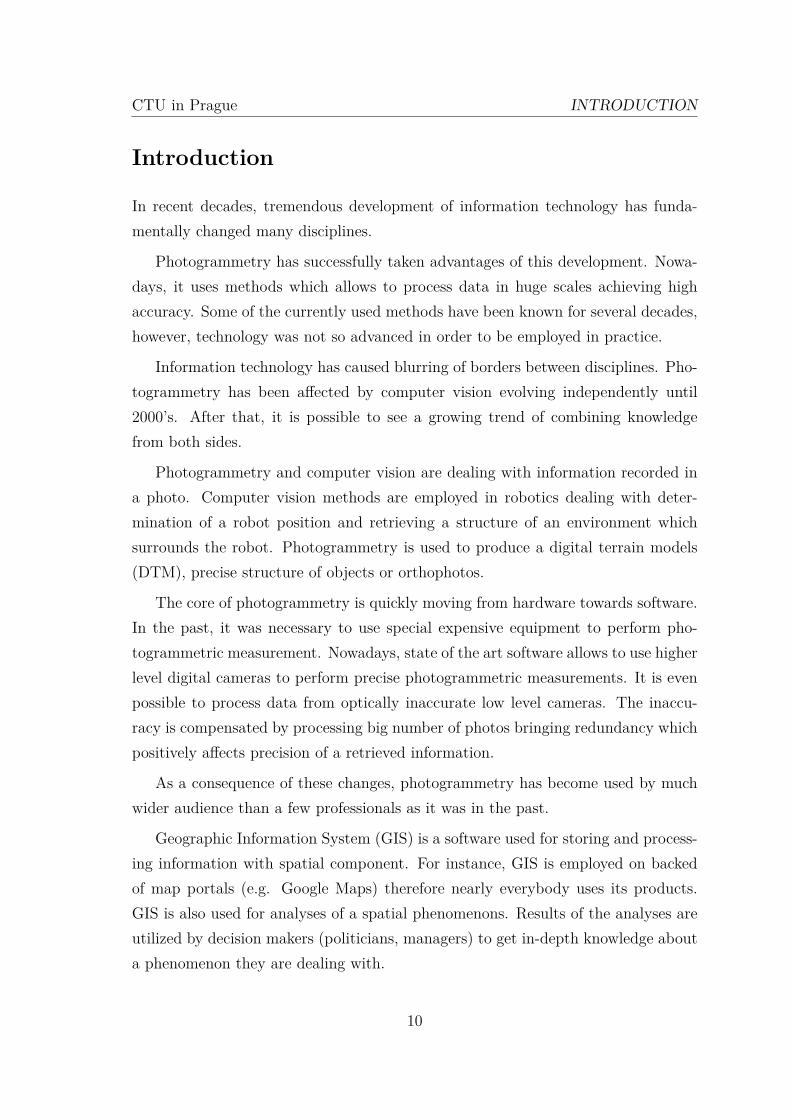
In recent decades, tremendous development of information technology has funda-mentally changed many disciplines.
Photogrammetry has successfully taken advantages of this development. Nowa-days, it uses methods which allows to process data in huge scales achieving highaccuracy. Some of the currently used methods have been known for several decades,however, technology was not so advanced in order to be employed in practice.
Information technology has caused blurring of borders between disciplines. Pho-togrammetry has been affected by computer vision evolving independently until2000’s. After that, it is possible to see a growing trend of combining knowledgefrom both sides.
Photogrammetry and computer vision are dealing with information recorded ina photo. Computer vision methods are employed in robotics dealing with deter-mination of a robot position and retrieving a structure of an environment whichsurrounds the robot. Photogrammetry is used to produce a digital terrain models(DTM), precise structure of objects or orthophotos.
The core of photogrammetry is quickly moving from hardware towards software.In the past, it was necessary to use special expensive equipment to perform pho-togrammetric measurement. Nowadays, state of the art software allows to use higherlevel digital cameras to perform precise photogrammetric measurements. It is evenpossible to process data from optically inaccurate low level cameras. The inaccu-racy is compensated by processing big number of photos bringing redundancy whichpositively affects precision of a retrieved information.
As a consequence of these changes, photogrammetry has become used by muchwider audience than a few professionals as it was in the past.
Geographic Information System (GIS) is a software used for storing and process-ing information with spatial component. For instance, GIS is employed on backedof map portals (e.g. Google Maps) therefore nearly everybody uses its products.GIS is also used for analyses of a spatial phenomenons. Results of the analyses areutilized by decision makers (politicians, managers) to get in-depth knowledge abouta phenomenon they are dealing with.
10
CTU in Prague INTRODUCTION
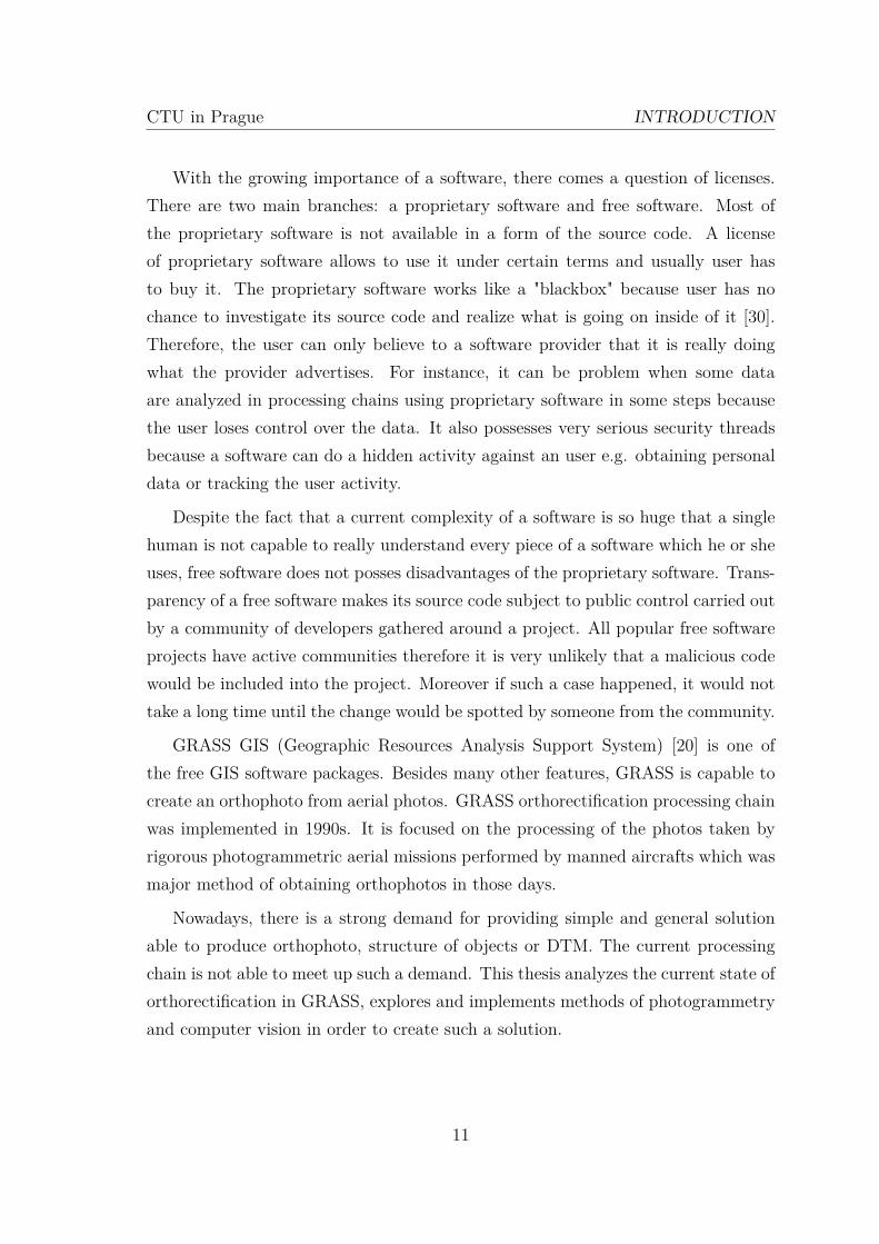
With the growing importance of a software, there comes a question of licenses.There are two main branches: a proprietary software and free software. Most ofthe proprietary software is not available in a form of the source code. A licenseof proprietary software allows to use it under certain terms and usually user hasto buy it. The proprietary software works like a "blackbox" because user has nochance to investigate its source code and realize what is going on inside of it [30].Therefore, the user can only believe to a software provider that it is really doingwhat the provider advertises. For instance, it can be problem when some dataare analyzed in processing chains using proprietary software in some steps becausethe user loses control over the data. It also possesses very serious security threadsbecause a software can do a hidden activity against an user e.g. obtaining personaldata or tracking the user activity.
Despite the fact that a current complexity of a software is so huge that a singlehuman is not capable to really understand every piece of a software which he or sheuses, free software does not posses disadvantages of the proprietary software. Trans-parency of a free software makes its source code subject to public control carried outby a community of developers gathered around a project. All popular free softwareprojects have active communities therefore it is very unlikely that a malicious codewould be included into the project. Moreover if such a case happened, it would nottake a long time until the change would be spotted by someone from the community.
GRASS GIS (Geographic Resources Analysis Support System) [20] is one ofthe free GIS software packages. Besides many other features, GRASS is capable tocreate an orthophoto from aerial photos. GRASS orthorectification processing chainwas implemented in 1990s. It is focused on the processing of the photos taken byrigorous photogrammetric aerial missions performed by manned aircrafts which wasmajor method of obtaining orthophotos in those days.
Nowadays, there is a strong demand for providing simple and general solutionable to produce orthophoto, structure of objects or DTM. The current processingchain is not able to meet up such a demand. This thesis analyzes the current state oforthorectification in GRASS, explores and implements methods of photogrammetryand computer vision in order to create such a solution.
11
CTU in Prague 1 THEORETICAL PART
1 Theoretical part
This chapter covers several methodological subtopics:
• essential principles of photogrammetry,
• the software framework in which the software has been developed within,
• mathematical background of least squares methods as used in photogramme-try,
• short introductions to photogrammetry and computer vision,
• an overview of bundle block adjustment (BBA) and orthorectification.
The purpose of this chapter is to introduce reader to methods used by photogram-metry and computer vision to retrieve DTM, orthophoto or structure of a capturedscene by group of photos. The chapter is focused especially on explanation of BBAmethod achieving the highest accuracy of retrieved products from photos. It alsoincludes description of all needed steps to obtain data required for performing BBA.Least square methods are covered by the chapter because they constitute the coreof BBA.
1.1 Essential principles
Photogrammetry and computer vision are dealing with a retrieving structure ofa scene from a group of photos capturing it. The structure retrieval methods arebased on pinhole camera model describing a relation of object point in 3D came-ra coordinate system and projected 2D photo point in photo coordinate system.Parameters characterizing pinhole camera model are called interior orientation.
Image plane is represented by a digital camera image sensor which creates photoconverting light into electronic signal. Then the signal is processed inside a cameragiving output in a form of photograph stored in a digital format. The image sensoris divided into cells measuring intensity of fallen light on their surface. A pixel valuein final photograph is based on the measured intensity of cell or group of cells. Thephoto created by image sensor is inverted. This kind of photo is called negative
12
CTU in Prague 1 THEORETICAL PART
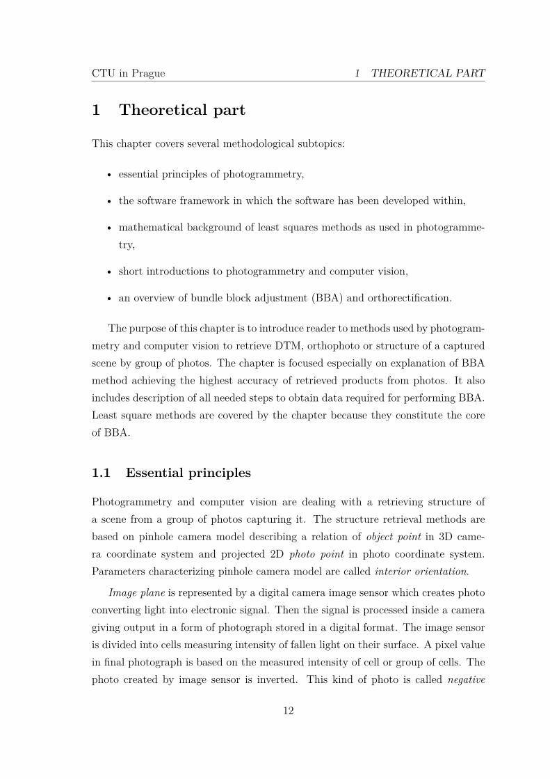
Figure 1: Pinhole camera model
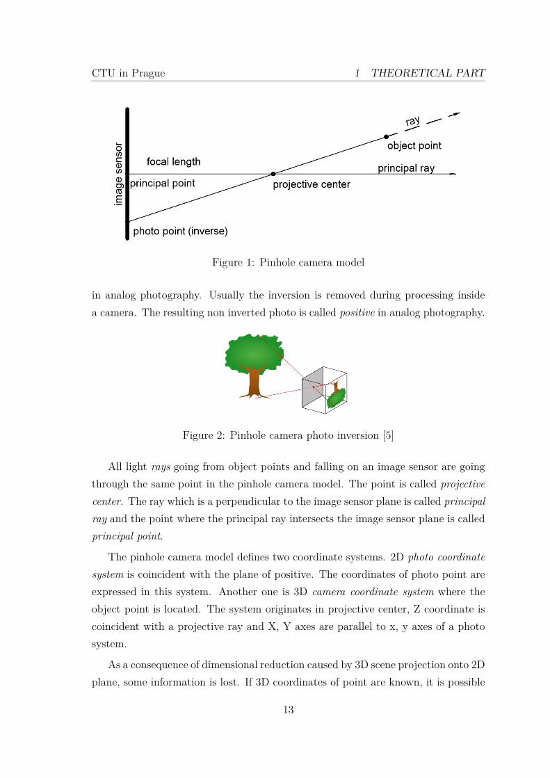
in analog photography. Usually the inversion is removed during processing insidea camera. The resulting non inverted photo is called positive in analog photography.
Figure 2: Pinhole camera photo inversion [5]
All light rays going from object points and falling on an image sensor are goingthrough the same point in the pinhole camera model. The point is called projectivecenter. The ray which is a perpendicular to the image sensor plane is called principalray and the point where the principal ray intersects the image sensor plane is calledprincipal point.
The pinhole camera model defines two coordinate systems. 2D photo coordinatesystem is coincident with the plane of positive. The coordinates of photo point areexpressed in this system. Another one is 3D camera coordinate system where theobject point is located. The system originates in projective center, Z coordinate iscoincident with a projective ray and X, Y axes are parallel to x, y axes of a photosystem.
As a consequence of dimensional reduction caused by 3D scene projection onto 2Dplane, some information is lost. If 3D coordinates of point are known, it is possible
13
CTU in Prague 1 THEORETICAL PART
to reproject it on the image sensor plane. Because of the dimensional reduction,only a ray can be reconstructed from a 2D photo point. 3D coordinates of a pointcan not be determined.
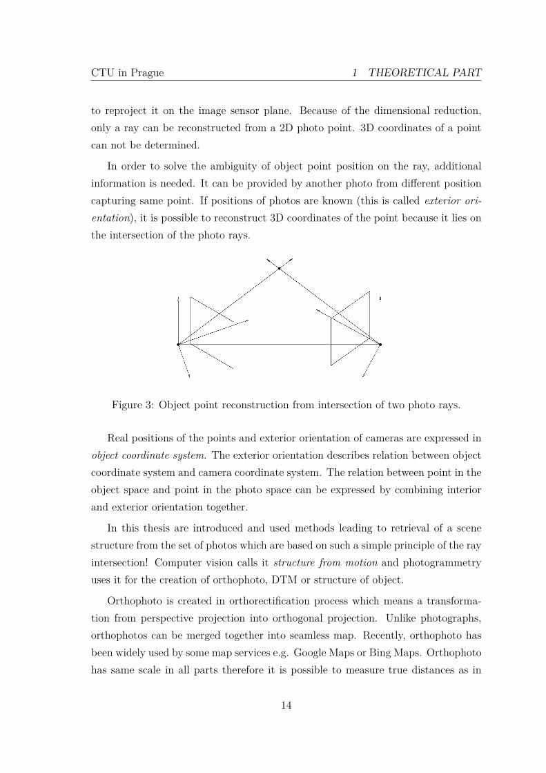
In order to solve the ambiguity of object point position on the ray, additionalinformation is needed. It can be provided by another photo from different positioncapturing same point. If positions of photos are known (this is called exterior ori-entation), it is possible to reconstruct 3D coordinates of the point because it lies onthe intersection of the photo rays.
Figure 3: Object point reconstruction from intersection of two photo rays.
Real positions of the points and exterior orientation of cameras are expressed inobject coordinate system. The exterior orientation describes relation between objectcoordinate system and camera coordinate system. The relation between point in theobject space and point in the photo space can be expressed by combining interiorand exterior orientation together.
In this thesis are introduced and used methods leading to retrieval of a scenestructure from the set of photos which are based on such a simple principle of the rayintersection! Computer vision calls it structure from motion and photogrammetryuses it for the creation of orthophoto, DTM or structure of object.
Orthophoto is created in orthorectification process which means a transforma-tion from perspective projection into orthogonal projection. Unlike photographs,orthophotos can be merged together into seamless map. Recently, orthophoto hasbeen widely used by some map services e.g. Google Maps or Bing Maps. Orthophotohas same scale in all parts therefore it is possible to measure true distances as in
14
CTU in Prague 1 THEORETICAL PART
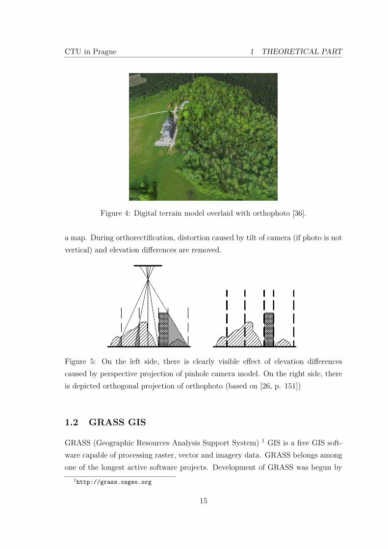
Figure 4: Digital terrain model overlaid with orthophoto [36].
a map. During orthorectification, distortion caused by tilt of camera (if photo is notvertical) and elevation differences are removed.
Figure 5: On the left side, there is clearly visible effect of elevation differencescaused by perspective projection of pinhole camera model. On the right side, thereis depicted orthogonal projection of orthophoto (based on [26, p. 151])
1.2 GRASS GIS
GRASS (Geographic Resources Analysis Support System) 1 GIS is a free GIS soft-ware capable of processing raster, vector and imagery data. GRASS belongs amongone of the longest active software projects. Development of GRASS was begun by
1http://grass.osgeo.org
15
CTU in Prague 1 THEORETICAL PART
the U.S. Army CERL laboratory (Construction Engineering Research Lab) in thefirst half of 1980s. In 1990s, U.S. Army gradually ceased developing GRASS. Luck-ily, the development could be taken over by volunteers because it had been decidedto release its source code as public domain. License of GRASS was changed intoGNU GPL v2 in 1999. GRASS is developed by the GRASS Development Teamcomprised of developers spread world wide.
Individual functionalities of GRASS are implemented in form of small softwarepackages called modules which can be combined together to solve complex tasks.Unlike other GIS systems as QGIS or ArcGIS, it takes more time for a new userto start understand the GRASS philosophy. Developers have been aware of thisproblem therefore they decided to develop a graphical user interface making GRASSmore friendly for beginners.
Data in GRASS are stored in so called GIS database composed of locations.Every location defines its projection thus all data belonging to the location must bereprojected to it. The location comprises mapsets used for organization of the datainto consistent units.
Another important element of GRASS is a computational region. The regionstores information about a geographical extent defined by four values (north, south,east, west) of a bounding box and another two values representing south-north andwest-east resolution. Properly set region is very important for raster data processingbecause nearly all raster modules performs computation on currently set region.Only exception are import raster modules ignoring it by default.
1.3 UAV
An unmanned aerial vehicle (UAV also known as drone) is aircraft without humanpilot. UAVs have been ingloriously known for heavy military employment especiallyby USA in Afghanistan and Pakistan. These military drones are equipped with stateof the art technology and their construction is similarly complex as a small aircraft.A number of military UAVs is quickly raising and nowadays USA trains more UAVoperators than fighter plane pilots.
Besides military UAVs, the sector of civil drones is exponentially growing. Itis very broad category ranging from big military like drones to small ones in size
16
CTU in Prague 1 THEORETICAL PART
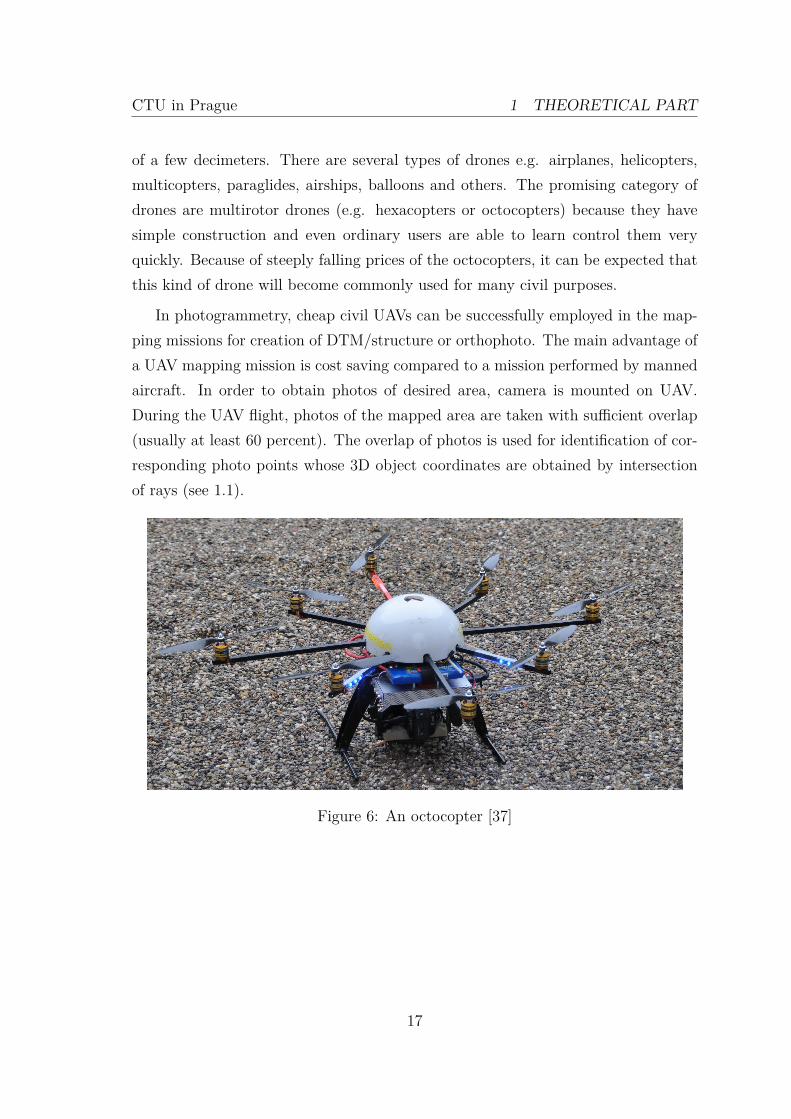
of a few decimeters. There are several types of drones e.g. airplanes, helicopters,multicopters, paraglides, airships, balloons and others. The promising category ofdrones are multirotor drones (e.g. hexacopters or octocopters) because they havesimple construction and even ordinary users are able to learn control them veryquickly. Because of steeply falling prices of the octocopters, it can be expected thatthis kind of drone will become commonly used for many civil purposes.
In photogrammetry, cheap civil UAVs can be successfully employed in the map-ping missions for creation of DTM/structure or orthophoto. The main advantage ofa UAV mapping mission is cost saving compared to a mission performed by mannedaircraft. In order to obtain photos of desired area, camera is mounted on UAV.During the UAV flight, photos of the mapped area are taken with sufficient overlap(usually at least 60 percent). The overlap of photos is used for identification of cor-responding photo points whose 3D object coordinates are obtained by intersectionof rays (see 1.1).
Figure 6: An octocopter [37]
17
CTU in Prague 1 THEORETICAL PART
1.4 Least squares
In linear algebra, commonly solved equation is:
AX = L (1)
It can be interpreted as:
• L - a vector of measurements,
• X - a vector of unknown parameters whose values are searched to solve (1),
• A - a matrix of a linear cost functions coefficients where row represents onemeasurement and column represents one coefficient of cost function. Lin-ear cost functions fi(X) represent relationship between measurements L andsearched parameters X. Least square method calls it a design matrix.
There is exactly one solution of vector of parameters X to satisfy the equationif matrix A is non singular matrix and vector b is not a zero vector. Non singularmatrix is always square matrix which has all column vectors and row vectors linearlyindependent.
Basically, every measurement is burden with some error. Errors can be dividedinto these main categories:
• gross error - it is caused by human factor or fault of the instrument. If themeasurement is repeated, usually, it is possible to identify measurements influ-enced by this error because they are big outliers from the other measurementsunaffected by this kind of error.
• systematic error - if measurement is repeated by the same instrument, it hassame effect (value) on the measurement. Usually effect of this error can beeliminated by choosing right measurement method, calibration of the instru-ment or taking it into account in a mathematic model.
• random error - this error is unavoidable because it is impossible to know per-fectly all factors which has impact on a measurement. The random errors
18
CTU in Prague 1 THEORETICAL PART
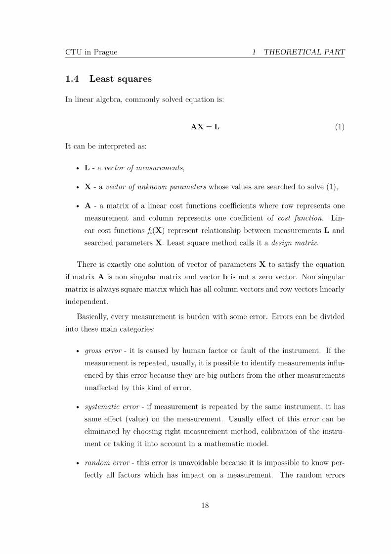
Figure 7: Density functions of normal distributions depending on values of standarddeviation σ and mean µ [35]
follow normal distribution represented by probability density function of thisshape.
The normal distribution is characterized by two parameters which are stan-dard deviation σ and mean µ. If measurements are burden only with randomerror, the mean represents accurate value and standard deviation representsdispersion level of measurements. Theoretically, if the measurements of someparameter would be repeated infinite times and the measurements would be in-fluenced only by random errors, accurate values could be computed as a mean.It follows that it is possible to get closer to the accurate value by repetition ofmeasurements leading into solving overdetermined systems. Another impor-tant implication is that the mean of the measurements performed by a moreaccurate instrument is statistically closer to the accurate value than the meanof same number of the measurements performed by a less precise instrument.Measurements of different accuracies can be combined together by weightedmean with weight of measurement pi defined as:
pi = constσ2i
(2)
where const is arbitrary chosen number used for calculation of all weights andσi is standard deviation of an instrument (representing accuracy) used for themeasurement.
19
CTU in Prague 1 THEORETICAL PART
The overdetermined systems are solved in many fields where final accuracy ofdetermined quantities by measurement (e.g. surveying, photogrammetry etc.) mat-ters.
As the consequence of overdetermination, the design matrix A becomes rectan-gular with more rows than columns and therefore the solution for linear equationssystem (1) does not exist. Only if the measurements were perfect it would be possibleto find such parameters vector X to solve the system of the linear equations.
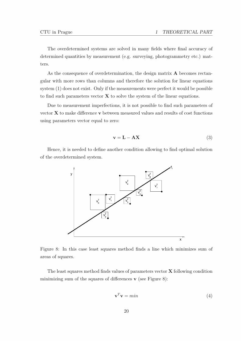
Due to measurement imperfections, it is not possible to find such parameters ofvector X to make difference v between measured values and results of cost functionsusing parameters vector equal to zero:
v = L−AX (3)
Hence, it is needed to define another condition allowing to find optimal solutionof the overdetermined system.
Figure 8: In this case least squares method finds a line which minimizes sum ofareas of squares.
The least squares method finds values of parameters vectorX following conditionminimizing sum of the squares of differences v (see Figure 8):
vTv = min (4)
20
CTU in Prague 1 THEORETICAL PART
The minimized square differences equation can be rewritten as:
vTv = (L−AX)T (L−AX)
= LTL− 2LTAX + XTATAX(5)
According to calculus notation, the least squares method searches for globalminimum of the square differences equation. The global minimum of a function canbe obtained using partial derivative of parameters in the cost function. In case oflinear cost functions, their square forms second degree polynomial e.g. parabola inR2, paraboloid in R3 etc. All these functions has only one point where all partialderivatives are equal to zero regardless dimension of the function. It is exactly theglobal minimum which the least squares method searches for!
The partial derivative of the minimized square differences equation can be writtenas [8]:
∂f (vTv)∂X
= −2ATL + 2ATAX (6)
The global minimum can be find by giving this equation equal to zero:
− 2ATL + 2ATAX = 0 (7)
The least square determines values of parameters vector X which can be ex-pressed from the previous equation:
X = (ATA)−1ATL (8)
It is essential equation of the least squares method. The equation can be solvedsimply by means of linear algebra.
The equation supposes that all measurements have same weight (accuracy). Theleast squares method can be extended to support weights. Weight matrix P containsweights of measurements on the diagonal with off-diagonal being zero elements ifthe measurements are not correlated.
The equation minimized by least squares is extended by the weight matrix intofollowing form:
vTPv = min (9)
21
CTU in Prague 1 THEORETICAL PART
Therefore, the essential least square equation is altered into this form:
X = (ATPA)−1ATPL (10)
1.4.1 Non-linear least squares
So far, it was supposed that the cost function is linear thus global minimum canbe found simply by means of linear algebra (10). Unfortunately, it is common thatthe relationship between parameters and measured values is not linear, hence, it isneeded to adapt linear least squares equations for non-linear cost functions.
Unlike linear least squares whose square of difference (5) is represented by func-tion (parabola, paraboloid...) with just one point where all partial derivatives arezero, the non-linear cost function can have many such points e.g. other local mini-mas.
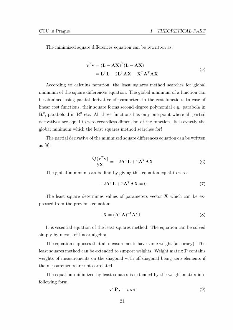
The problem of non-linearity can be solved by linearization of non-linear equa-tions. The main idea of linearization process is to approximate the cost functionwith first degree Taylor polynomial, which is linear. Therefore, it is possible to uselinear least square equation (10) to solve non-linear problem.
Figure 9: Function fi is approximated by first degree Taylor polynomial T fi , formingline in R2. Symbol ∆ represents an approximation error.
Approximation of the cost function by a first degree Taylor polynomial can bewritten as [44]:
T fi,X01 (X) = fi(X0) + ∂
∂X01
fi(X0)(X−X0) ... + ∂
∂X0n
fi(Xn)(X−X0) (11)
22
CTU in Prague 1 THEORETICAL PART
where:
• X0 is a point where the Taylor polynomial touches approximated function. Forinstance, first degree Taylor polynomial is a line which is a tangent of functionat the point X0 in R2, tangent plane in R3 and tangent hyperplane in Rn.
• X is a point where the Taylor polynomial returns approximate value of thecost function fi.
Least squares Taylor polynomial can be written as:
T fi,X01 (X) = fi(X0) + a0dx0 ... + andxn (12)
It can be rewritten into a matrix form with formal substitution LX0 = fi(X0):
T fi,X01 (X) = LX0 + Adx (13)
It should be noted that the design matrix A contains partial derivatives of costfunctions. Analogous equation to (3) can be derived:
v = L− T fi,X01 (X) (14)
Taylor polynomial member can be expanded by (13):
v = L− LX0 −Adx
= l−Adx(15)
If the differences vector from the previous equation is substituted into leastsquares minimization criterion:
vTPv = min (16)
The essential equation for non linear least squares can be derived similarly tolinear least squares:
dx = (ATPA)−1ATPl
X = dx + X0(17)
23
CTU in Prague 1 THEORETICAL PART
The equation is slightly different compared to the linear least squares equation(10). Instead of the parameters vector X, result of the equation is correction vectorof parameters dx. Measurement vector L is analogous to vector l. In this two minorsubstitutions, there are hidden major limitations of the non-linear least squaresmethod where the price for the approximation is paid.
As it was already mentioned, the Taylor polynomial is tangent of approximatedat point X0. This approximation is good in close surroundings of the point X0,however, as the distance grows, the approximation error ∆ may increase significantlywhich can be clearly seen in Figure 9.
Therefore, unlike linear least square method, non-linear least squares requiresinitial values of parameters X. If the initial values are not accurate enough, it ispossible to iteratively run linear least squares subsequently. In the new iteration,adjusted parameters vector X from the previous iteration is used to eventually ap-proach global minimum of the cost function. Therefore the closeness of the initialpoint X0 to global minimum affects how many iterations (speed of convergence) areneeded to achieve optimal solution (global minimum).
Unfortunately, the non-linear least square method has another one, even moreserious pitfall which does not guarantee that it will iterate towards global minimumat all! In such a case, the found values of parameters vector X are completelywrong because it does not satisfies minimum squares difference condition (16). Ifthe initial values are inaccurate, the method can iterate toward other points withzero derivation (e.g. local minimums). This is caused by run-off of minimizedfunction created from non-linear cost function which can have more points withzero derivative unlike the minimized function by linear least squares method.
Therefore, success of non-linear least squares method depends on the initialvalues of parameters vector X!
1.4.2 Least squares properties
It was proved [17] that above derived least square method is solution of Gauss-Markoff model which says: If measurements L are random with known covariancematrix Σl and vector of unknown parameters X is non-random then vector dxhas the lowest variance and it is unbiased. If density functions of measurements
24
CTU in Prague 1 THEORETICAL PART
are normally distributed (see Figure 7) then values obtained from the cost functionsusing computed parameters lies in maximum of the density function. In other words,they posses maximum likelihood.
The weight matrix is calculated from covariance matrix in similar way as weightsin weighted mean (2):
P = constΣ2i
(18)
Where const is chosen arbitrary. It can be selected as a priori standard deviationof unit weight σ0.
Unbiased unit weight standard deviation σ0 can be also estimated a posteriorias:
σ20 = vTPv
r (19)
Where r is redundancy which is difference of columns number from rows numberof design matrix A.
Covariance of calculated parameters Σx can be get from:
Σx = σ20(ATPA)−1 (20)
A posteriori covariance matrix Σl of measurements can be obtained from:
Σl = AΣxAT (21)
1.4.3 Iteration termination
Non-linear least squares method is iterative, thus it is needed define some criteriaallowing to assess whether global minimum was reached.
The criterion [19] can be based on assessment of parameters corrections dx. Forinstance, it can be chosen threshold of maximum absolute value of correction. If thethreshold is not satisfied another iteration is performed.
Another criterion is maximum number of iterations. The criterion is importantin cases when the least squares method is unable to converge to some point resultingin impossibility to satisfy the previous criterion.
Thus, this criterion prevents from falling into infinite loop. The threshold cannot be chosen too small in order to least squares method has enough iteration toconverge to global minimum.
25
CTU in Prague 1 THEORETICAL PART
1.4.4 Free network least squares
In geodesy, it can happen that columns of design matrix A are not linearly inde-pendent. It can be caused by datum deficiency [6]. The datum deficiency is missinginformation about coordinate system of the network in the design matrix [34]. Itmakes normal matrix ATPA non invertible because of linearly dependent columnsof design matrix. Thus, the least squares equation (17) can not be solved. In orderto avoid the datum deficiency issue, it is needed to keep some parameters fixed whichmeans that columns of the fixed parameters are excluded from design matrix A.
Photogrammetry deals with three dimensional space requiring at least two pointsto be fixed with another point with one coordinate to avoid datum deficiency problembecause three dimensional coordinate system is defined by three coordinates of shiftvector, three rotation angles and scale factor.
If there are not enough fixed points, a network has to be adjusted as a freenetwork. One of possible methods how to adjust a free network is calculation ofpseudo inverse matrix of the normal matrix instead of inverse. Another option isadding inner constraints to the least squares system.
1.5 Short introduction to photogrammetry
Essential information which must be known to obtain any photogrammetric product(e.g. orthophoto or DTM) from group of the photos is their interior orientation andexterior orientation. Exterior and interior orientation together describe relationbetween a 3D object point and corresponding 2D photo point.
1.5.1 Interior orientation
Interior orientation describes relation between photo coordinate system and corre-sponding 3D camera-related coordinate system which is based on pinhole cameramodel described in the chapter 1.1.
Photogrammetric camera coordinate system has origin in projective point, z axisheading out of the scene and x, y axes being parallel to the photo plane. Directionsof x, y axes are selected in way to be the camera system right handed.
26
CTU in Prague 1 THEORETICAL PART
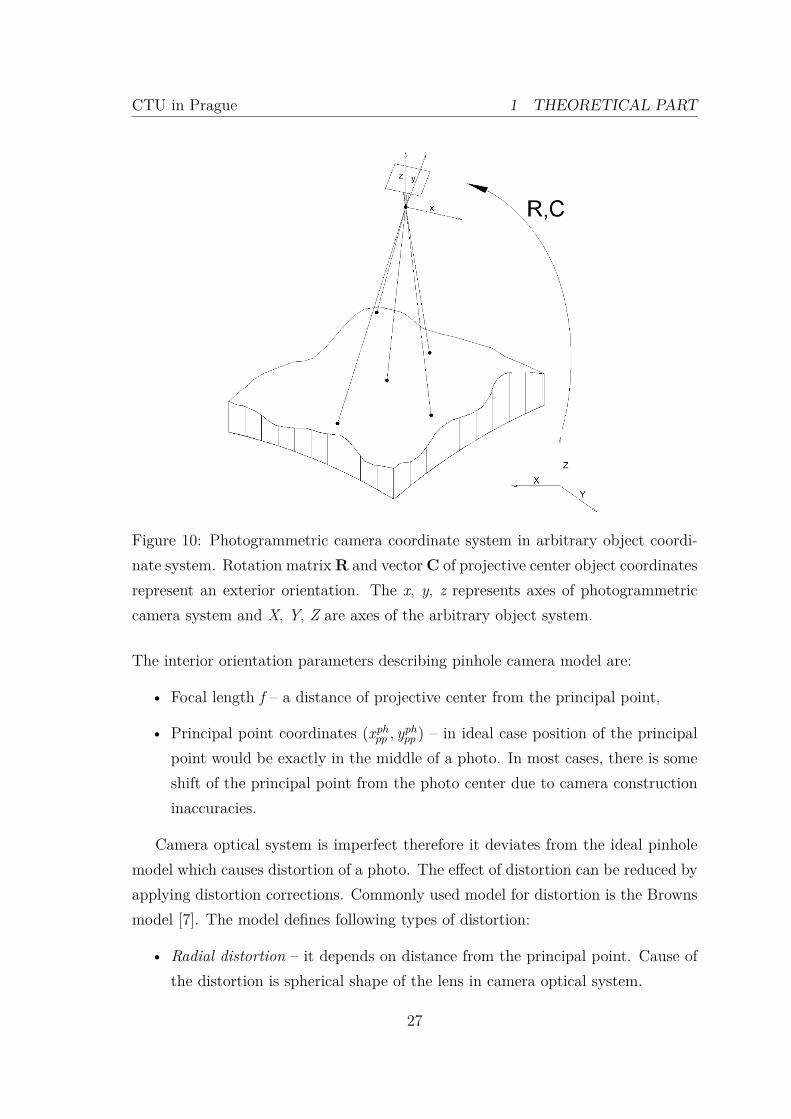
Figure 10: Photogrammetric camera coordinate system in arbitrary object coordi-nate system. Rotation matrixR and vectorC of projective center object coordinatesrepresent an exterior orientation. The x, y, z represents axes of photogrammetriccamera system and X, Y, Z are axes of the arbitrary object system.
The interior orientation parameters describing pinhole camera model are:
• Focal length f – a distance of projective center from the principal point,
• Principal point coordinates (xphpp , yphpp ) – in ideal case position of the principalpoint would be exactly in the middle of a photo. In most cases, there is someshift of the principal point from the photo center due to camera constructioninaccuracies.
Camera optical system is imperfect therefore it deviates from the ideal pinholemodel which causes distortion of a photo. The effect of distortion can be reduced byapplying distortion corrections. Commonly used model for distortion is the Brownsmodel [7]. The model defines following types of distortion:
• Radial distortion – it depends on distance from the principal point. Cause ofthe distortion is spherical shape of the lens in camera optical system.
27
CTU in Prague 1 THEORETICAL PART
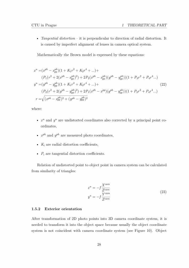
• Tangential distortion – it is perpendicular to direction of radial distortion. Itis caused by imperfect alignment of lenses in camera optical system.
Mathematically the Brown model is expressed by these equations:
xu =(xph − xphpp )(1 + K1r2 + K2r
4 + ...)+
(P1(r2 + 2(xph − xphpp )2) + 2P2(xph − xphpp )(yph − yphpp ))(1 + P3r2 + P4r
4...)
yu =(yph − yphpp )(1 + K1r2 + K2r
4 + ...)+
(P2(r2 + 2(yph − yphpp )2) + 2P1(xph − xpp)(yph − yphpp ))(1 + P3r2 + P4r
4...)
r =√
(xph − xphpp )2 + (yph − yphpp )2
(22)
where:
• xu and yu are undistorted coordinates also corrected by a principal point co-ordinates,
• xph and yph are measured photo coordinates,
• Ki are radial distortion coefficients,
• Pi are tangential distortion coefficients.
Relation of undistorted point to object point in camera system can be calculatedfrom similarity of triangles:
xu = −f X cam
Z cam
yu = −f Y cam
Z cam
(23)
1.5.2 Exterior orientation
After transformation of 2D photo points into 3D camera coordinate system, it isneeded to transform it into the object space because usually the object coordinatesystem is not coincident with camera coordinate system (see Figure 10). Object
28

CTU in Prague 1 THEORETICAL PART
space coordinate system must be Cartesian otherwise it must be transformed intoCartesian one before applying equations derived bellow.
Exterior orientation is defined by position of camera projective center in theobject space and the orientation of the camera coordinate system in the object space.Photogrammetry uses representation of orientation by Euler angles and rotationmatrix. The Euler angles are group of three angles, which describes three subsequentrotations around axes of 3D coordinate system. Order of Euler angles is importantbecause, if it is breached, resulting orientation is different. In this work, there isused BLUH notation [3] where rotation around y axis by angle ϕ is perform at first,then system is rotated around x axis by angle ω and the last rotation is performaround z axis by angle κ.
The three Euler rotations can be mathematically expressed as multiplication ofthree corresponding rotation matrices:
R = Rz(κ)Rx(ω)Ry(ϕ)
=
cos(κ) sin(κ) 0−sin(κ) cos(κ) 0
0 0 1
1 0 00 cos(ω) sin(ω)0 −sin(ω) cos(ω
cos(ϕ) 0 −sin(ϕ)
0 1 0sin(ϕ) 0 cos(ϕ)
= cos(κ)cos(ϕ) + sin(κ)sin(ω)sin(ϕ) sin(κ)cos(ω) −cos(κ)sin(ϕ) + sin(κ)sin(ω)cos(ϕ)−sin(κ)cos(ϕ) + sin(κ)sin(ω)sin(ϕ) cos(κ)cos(ω) sin(κ)sin(ϕ) + cos(κ)sin(ω)cos(ϕ)
cos(ω)sin(ϕ) −sin(ω) cos(ω)cos(ϕ)
(24)
BLUH angles can be retrieved from rotation matrix by following equitations:
ϕ = arctan(R31
R33
)
ω = arctan
−R32√R2
12 + R222
κ = arctan
(C12
R22
)(25)
Arctangent should be calculated with the function giving final angle into properquadrant, according to sings of numerator and denominator. Usually, this functionsis called atan2.
Pitfall of the Euler angles is when value of the second Euler angle is 90 or 270degrees, then Euler angles representation is singular, which is called gimbal lock. If
29
CTU in Prague 1 THEORETICAL PART
values of Euler angles are close to the gimbal lock, it could cause serious numericalinstabilities.
The rotation matrix represents three subsequent rotations of an object systemto be oriented as a camera system.
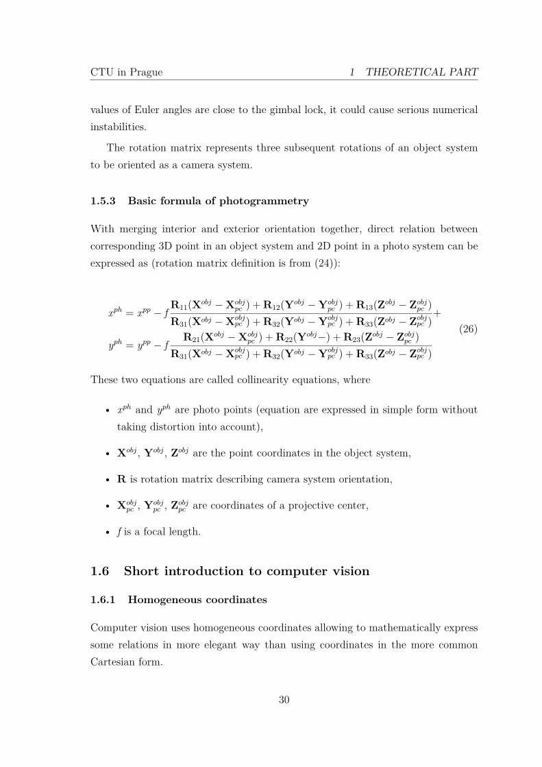
1.5.3 Basic formula of photogrammetry
With merging interior and exterior orientation together, direct relation betweencorresponding 3D point in an object system and 2D point in a photo system can beexpressed as (rotation matrix definition is from (24)):
xph = xpp − fR11(Xobj −Xobj
pc ) + R12(Yobj −Yobjpc ) + R13(Zobj − Zobj
pc )R31(Xobj −Xobj
pc ) + R32(Yobj −Yobjpc ) + R33(Zobj − Zobj
pc )+
yph = ypp − fR21(Xobj −Xobj
pc ) + R22(Yobj−) + R23(Zobj − Zobjpc )
R31(Xobj −Xobjpc ) + R32(Yobj −Yobj
pc ) + R33(Zobj − Zobjpc )
(26)
These two equations are called collinearity equations, where
• xph and yph are photo points (equation are expressed in simple form withouttaking distortion into account),
• Xobj, Yobj, Zobj are the point coordinates in the object system,
• R is rotation matrix describing camera system orientation,
• Xobjpc , Yobj
pc , Zobjpc are coordinates of a projective center,
• f is a focal length.
1.6 Short introduction to computer vision
1.6.1 Homogeneous coordinates
Computer vision uses homogeneous coordinates allowing to mathematically expresssome relations in more elegant way than using coordinates in the more commonCartesian form.
30
CTU in Prague 1 THEORETICAL PART
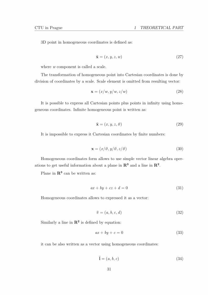
3D point in homogeneous coordinates is defined as:
x = (x , y, z ,w) (27)
where w component is called a scale.
The transformation of homogeneous point into Cartesian coordinates is done bydivision of coordinates by a scale. Scale element is omitted from resulting vector:
x = (x/w, y/w, z/w) (28)
It is possible to express all Cartesian points plus points in infinity using homo-geneous coordinates. Infinite homogeneous point is written as:
x = (x , y, z , 0 ) (29)
It is impossible to express it Cartesian coordinates by finite numbers:
x = (x/0 , y/0 , z/0 ) (30)
Homogeneous coordinates form allows to use simple vector linear algebra oper-ations to get useful information about a plane in R3 and a line in R2.
Plane in R3 can be written as:
ax + by + cz + d = 0 (31)
Homogeneous coordinates allows to expressed it as a vector:
π = (a, b, c, d) (32)
Similarly a line in R2 is defined by equation:
ax + by + c = 0 (33)
it can be also written as a vector using homogeneous coordinates:
l = (a, b, c) (34)
31
CTU in Prague 1 THEORETICAL PART
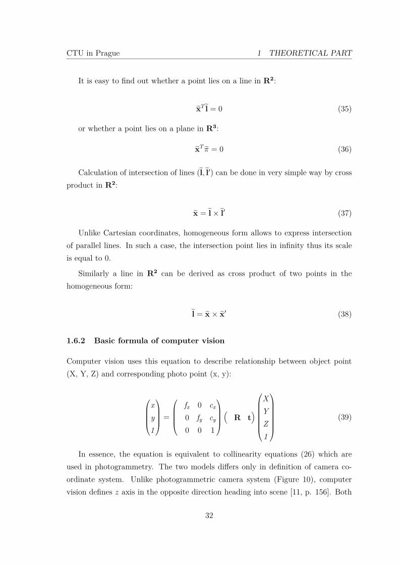
It is easy to find out whether a point lies on a line in R2:
xT l = 0 (35)
or whether a point lies on a plane in R3:
xT π = 0 (36)
Calculation of intersection of lines (l, l′) can be done in very simple way by crossproduct in R2:
x = l× l′ (37)
Unlike Cartesian coordinates, homogeneous form allows to express intersectionof parallel lines. In such a case, the intersection point lies in infinity thus its scaleis equal to 0.
Similarly a line in R2 can be derived as cross product of two points in thehomogeneous form:
l = x× x′ (38)
1.6.2 Basic formula of computer vision
Computer vision uses this equation to describe relationship between object point(X, Y, Z) and corresponding photo point (x, y):
xy1
=
fx 0 cx
0 fy cy
0 0 1
( R t)
XYZ1
(39)
In essence, the equation is equivalent to collinearity equations (26) which areused in photogrammetry. The two models differs only in definition of camera co-ordinate system. Unlike photogrammetric camera system (Figure 10), computervision defines z axis in the opposite direction heading into scene [11, p. 156]. Both
32
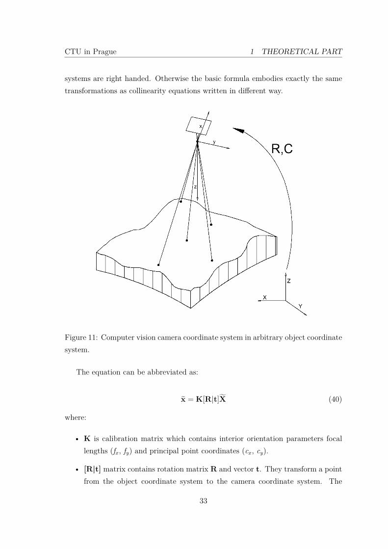
CTU in Prague 1 THEORETICAL PART
systems are right handed. Otherwise the basic formula embodies exactly the sametransformations as collinearity equations written in different way.
Figure 11: Computer vision camera coordinate system in arbitrary object coordinatesystem.
The equation can be abbreviated as:
x = K[R|t]X (40)
where:
• K is calibration matrix which contains interior orientation parameters focallengths (fx, fy) and principal point coordinates (cx, cy).
• [R|t] matrix contains rotation matrix R and vector t. They transform a pointfrom the object coordinate system to the camera coordinate system. The
33
CTU in Prague 1 THEORETICAL PART
vector t can be transformed by:
C = −RT t (41)
giving coordinates of camera projective center in object space. The rotationmatrix R and the projective center object coordinates C represent exteriororientation of the camera.
• X homogeneous coordinates of an object point,
• x homogeneous coordinates of transformed photo point.
Whole projection can be merged into single matrix P called camera matrix:
x = PX = K[R|t]X (42)
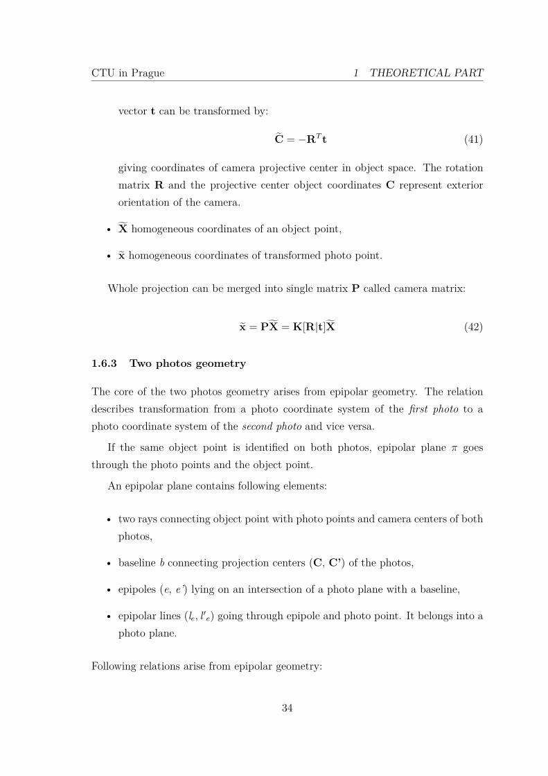
1.6.3 Two photos geometry
The core of the two photos geometry arises from epipolar geometry. The relationdescribes transformation from a photo coordinate system of the first photo to aphoto coordinate system of the second photo and vice versa.
If the same object point is identified on both photos, epipolar plane π goesthrough the photo points and the object point.
An epipolar plane contains following elements:
• two rays connecting object point with photo points and camera centers of bothphotos,
• baseline b connecting projection centers (C, C’) of the photos,
• epipoles (e, e’) lying on an intersection of a photo plane with a baseline,
• epipolar lines (le, l ′e) going through epipole and photo point. It belongs into aphoto plane.
Following relations arise from epipolar geometry:
34
CTU in Prague 1 THEORETICAL PART
Figure 12: Epipolar geometry.
• All epipolar lines of photo intersect in a epipole. Epipoles lie at infinity if thephotos are merely translated with no difference in orientation.
• A photo point forms epipolar line in the other photo. It allows to reduce spaceof possible occurrence of the point from R2 to R1 of epipolar line withoutsome other information about the point e.g. object space coordinates.
Camera matrix P (42) represents projective transformation from object systemto the first photo system. Reversed transformation can not be done by inverse matrixbecause of the rectangular shape (3x4) of camera matrix P. Instead of matrix inver-sion, pseudo inverse matrix P+ must be calculated to reverse the transformation.Pseudo inverse matrix has this property: PP+ = I. Singularity of the matrix canbe interpreted as consequence of information loss caused by dimensional reductiondone by transformation of 3D object point into 2D photo plane.
A point x of the first photo system can be transformed into the second photosystem as point x′ by:
x′ = P′P+x (43)
where P and P’ are camera matrices of the first and the second photo.
35
CTU in Prague 1 THEORETICAL PART
The transformed point x′ lies at infinity representing direction of a epipolar linel ′e. A line can be define by a direction and a point. In order to define epipolarline l ′e missing point can be obtained from projection of the first camera projectivecenter C into the second photo system where it represent epipole:
e′ = P′C (44)
Epipolar line is given (37) by:
l′e = e′ ×P′P+x = (P′C)×P′P+x (45)
Cross product of two vectors a and b can be also written as multiplication of amatrix and a vector:
a × b =
0 a3 a2
a3 0 −a1
−a2 a1 0
b = [a]×b (46)
The epipolar line equation can be rewritten using the matrix notation of crossproduct as:
l′e = [e′]×P′P+x (47)
It is apparent from the equation that matrix denoting relation of two photos isdefined as:
F = [e′]×P′P+ (48)
Matrix F is called a fundamental matrix [11]. It transforms photo points of thefirst photo system into epipolar lines of the second photo system. Fundamentalmatrix can be expanded by (42). It allows to derive another important matrix oftwo view geometry called essential matrix E.
Lets suppose that camera matrix of the first photo is defined in this way:
P = K[I|0] (49)
It means that the first camera coordinate system coincides with the object spacecoordinate system.
36
CTU in Prague 1 THEORETICAL PART
Its pseudo inverse matrix is:
P+ =K−1
0T
(50)
Homogeneous object projective center coordinates are:
C =0
1
(51)
The second camera matrix is defined in this way:
P′ = K′[R|t] (52)
Epipole of the second photo is given as:
e′ = P′0
1
= K′t
(53)
The relationship of two cameras is also called relative orientation, because rota-tion matrix R and vector t represents orientation and position of the second camerato the first one. This relationship is defined up to scale. In order to express camerasexterior orientations in a world coordinate system or merge it with another relativeorientations, it is needed to perform further transformations of the relative exteriororientations, for more information see chapters 1.6.6 and 1.6.7.
The fundamental matrix equation can be rewritten taking into account the rel-ative orientation (50), (51), (52) and (53) as:
F = [P′C]×P′P+ = [K′[R|t]0
1
]×K′[R|t]K−1
0T
= [K′t]×K′RK−1
= [e′]×K′RK−1
(54)
Now, there comes little bit more difficult part. This formula applies for anynon-singular matrix M and vector x [11, p. 582]:
[x]×M = M−T [M−1x]× (55)
37
CTU in Prague 1 THEORETICAL PART
The fundamental matrix equation can be further rewritten using the formulas(55) and (53):
F = [e′]×K′RK−1
= K′−T [K′−1e′]×RK−1
= K′−T [K′−1K′t]×RK−1
= K′−T [t]×RK−1
(56)
This equation reveals very important fact about fundamental matrix saying thata transformation performed by matrix can be divided into a three main steps.
In first step, photo coordinates of point are normalized. Normalized coordinatesof the first photo are transformed into normalized coordinates of the second photoby essential matrix:
E = [t]×R (57)
Eventually, the coordinates are transformed into photo system of the secondphoto representing epipolar line.
It follows that the essential matrix incorporates a relative orientation of two pho-tos. Essential matrix is subset of whole information encoded in fundamental matrix.Fundamental matrix includes additional information about interior orientations ofcameras which took the photos.
Hence, if exterior orientation of a two photos is known, the essential matrix canbe computed. The matrix can be calculated from exterior orientations independentlyof specific object coordinates system since it takes into account the relative positionof two photos up to scale. Moreover, if calibration matrices are known, it is possibleto define a relationship (without taking into account distortion) between the twophoto systems by fundamental matrix.
1.6.4 Triangulation of points
Triangulation methods deal with retrieval of the object point coordinates from cor-responding points in photos. If measurements would be precise, object point wouldlie on intersection of two rays which is clearly visible in Figure 3. Unfortunately the
38
CTU in Prague 1 THEORETICAL PART
rays are never determined so precisely to intersect. Several methods deals with theimperfections.
One of them is direct linear transformation (DLT) method based on linearizationof collinearity equations (26) employing least squares method on it.
The simplified DLT form of collinearity equations can be written as [25, p. 130]:
xun = a1(Xobj) + a2(Yobj) + a3(Zobj) + a4
a9(Xobj) + a10(Yobj) + a11(Zobj) + 1
yun = a5(Xobj) + a6(Yobj) + a7(Zobj) + a8
a9(Xobj) + a10(Yobj) + a11(Zobj) + 1
(58)
It can be expressed in linear form:
xph =a1Xobj + a2Yobj + a3Zobj + a4
− xpha9Xobj − xpha10Yobj − xpha11Zobj
yph =a5Xobj + a6Yobj + a7Zobj + a8
− ypha9Xobj − ypha10Yobj − ypha11Zobj
(59)
Because of linearity, it does not require to know approximate values. Maindrawback of this method is that DLT model does not respect pinhole camera modelthus minimized parameters in the vector a do not follow rigorous camera geometrywhich may result in inaccurate retrieval of object coordinates. Another problem ofthe method is that it is not fully linear because variables xph and yph occurs also inthe right side of the equations.
More rigorous method is called the optimal solution. It is based on enforcingepipolar constraint. The cost function minimizes sum of squares of distances be-tween photo points and epipolar lines. The lines are created by transformation ofcorresponding photo points from another photos.
The cost function is not linear, however, it’s derivative leads into 6 degree polyno-mial thus it has 6 roots. Correct solution can be selected from roots by assumptionthat it represents global minimum.
This method is considered by computer vision community as the most accurate[11, p. 315].
39
CTU in Prague 1 THEORETICAL PART
1.6.5 Retrieving of relative orientation from essential matrix
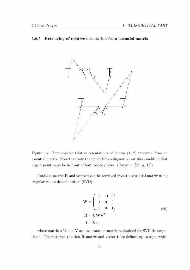
Figure 13: Four possible relative orientations of photos (1, 2) retrieved from anessential matrix. Note that only the upper left configuration satisfies condition thatobject point must be in front of both photo planes. (Based on [28, p. 19])
Rotation matrix R and vector t can be retrieved from the essential matrix usingsingular values decomposition (SVD):
W =
0 −1 01 0 00 0 1
R = UWVT
t = U3,:
(60)
where matrices U and V are two rotation matrices obtained for SVD decompo-sition. The retrieved rotation R matrix and vector t are defined up to sign, which
40
CTU in Prague 1 THEORETICAL PART
causes four case ambiguity.
As a consequence of the ambiguity it gives four relative orientations:
[R|t], [R|−t], [−R|t], [−R|−t], (61)
The correct solution can be found by assumption that all object points has tobe in the front of the both photo planes.
1.6.6 Merging of relative orientations
If two relative orientations are merged together, they must share one photo. As a firststep, it is necessary to calculate a scale [28] because relative orientation coordinatesystems are independent of scale. The scale can be calculated from correspondingdistances measurable in both coordinate systems. Distances between object pointdetermined in both camera systems and object coordinates of the projective centerof shared photo can be used for calculation of scale:
sro2−1 = ||Xro11 −Cro1
1 ||||Xro2
1 −Cro21 ||
(62)
where:
• ro1, ro2 are relative orientation coordinate systems. System ro2 is transformedinto system ro1,
• X is an object point determined in both relative orientations,
• C is a projective center of the shared photos.
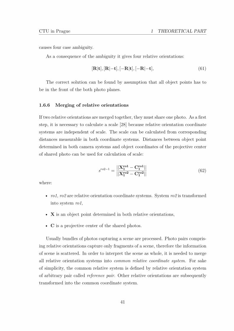
Usually bundles of photos capturing a scene are processed. Photo pairs compris-ing relative orientations capture only fragments of a scene, therefore the informationof scene is scattered. In order to interpret the scene as whole, it is needed to mergeall relative orientation systems into common relative coordinate system. For sakeof simplicity, the common relative system is defined by relative orientation systemof arbitrary pair called reference pair. Other relative orientations are subsequentlytransformed into the common coordinate system.
41
CTU in Prague 1 THEORETICAL PART
Figure 14: In the left picture, there are relative orientations ro1, ro2 before transfor-mation to a common system. In the right picture, there is common system definedby ro1 after transformation of ro2. Note change of ro2 scale after the transformation.(Based on [28, p. 20])
All relative orientations which can be transformed into common system form con-nected component of undirected graph. Nodes represents photos and edges denotesrelative orientations. In other words, it is possible to transform relative orientationinto the common relative coordinate system only, if there is a continuous chain ofthe relative orientations from reference pair to the transformed orientation, whereevery two neighborhood relative orientations in the chain share one photo.
The transformation of relative orientations 1-n into common system defined byrelative orientation 1 can be written as:
P1_co = [I|O]
P2_co = [Rro1|tro1] = [Rro1_co|tro1_co]
P3_co = [Rro2Rro1_co|Rro2tro1_co + sro2−1tro2] = [Rro3_co|tro3_co]
Pn_co = [Rro(n)Rro(n−1)_co|Rro(n)tro(n−1)_co + sro(n)−(n−1)tro(n)] = [Rro(n)_co|tro(n)_co](63)
The equations suppose that camera matrices in ro(n) relative orientation systemare defined as Pn = [I|O] and Pn+1 = [Rro(n)|tro(n)].
42
CTU in Prague 1 THEORETICAL PART
1.6.7 Helmert transformation
Helmert transformation can be written by equation:
Xt = t + sRX (64)
where R is a rotation matrix, s is a scale scalar, t is a translation vector andX is transformed point into a point Xt. The transformation is defined by sevenparameters (three translation coordinates, three rotation angles and scale). In orderto get these parameters it is needed to know at least two corresponding points andanother one with at least one known coordinate in both coordinate systems.
Helmert transformation parameters can be retrieved from corresponding pointsby several methods. For instance closed form method can be employed based onSVD decomposition [32].
1.7 Bundle block adjustment
Bundle block adjustment (BBA) is a method which uses the least squares technique(1.4) to refine scene parameters. The main advantage of BBA is that the it takes intoaccount whole scene and therefore it utilizes maximum information for adjustment ofscene parameters which leads to the more accurate results. The principle of BBA hasbeen known for very long time since 1950s, however, the method has been employedin practical applications since 1990’s because the performance of computers had notbeen sufficient enough before.
The cost functions of BBA least squares method are photogrammetric collinearityequations (26). The least squares method tries to find vector of adjusted parametersX to minimize sum of square differences between coordinates of measured photopoints and photo points calculated from collinearity equations.
Unfortunately, collinearity equations are non linear hence the non-linear leastsquare method (1.4.1) must be employed, which needs to be provided with suffi-ciently accurate initial values in order to find values of parameters satisfying mini-mization criterion.
Thanks to the least squares method, BBA is very flexible in terms of selectionof the parameters to be adjusted. It is possible to select various combinations of
43
CTU in Prague 1 THEORETICAL PART
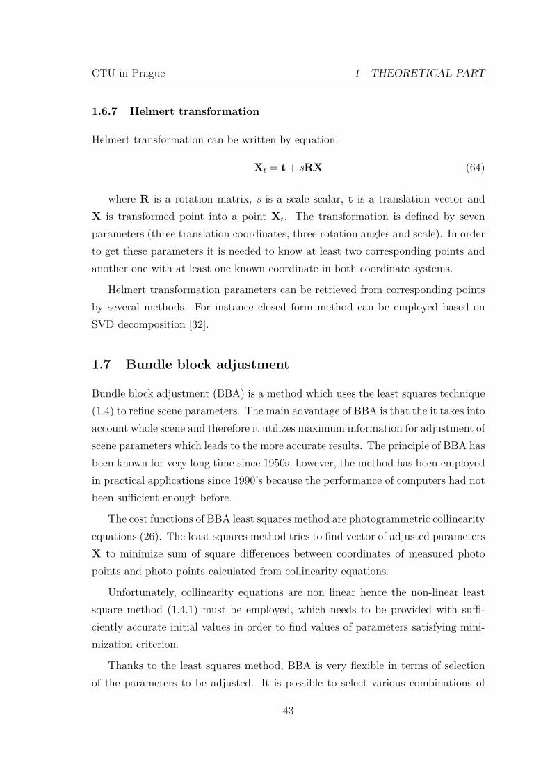
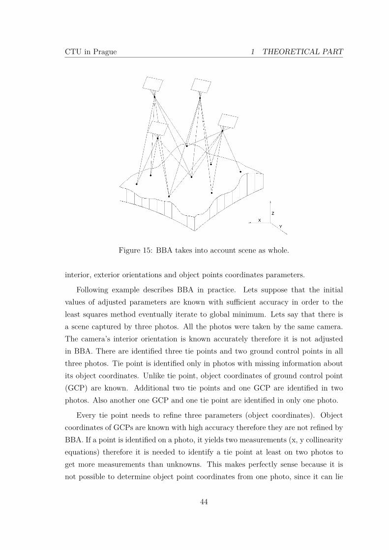
Figure 15: BBA takes into account scene as whole.
interior, exterior orientations and object points coordinates parameters.
Following example describes BBA in practice. Lets suppose that the initialvalues of adjusted parameters are known with sufficient accuracy in order to theleast squares method eventually iterate to global minimum. Lets say that there isa scene captured by three photos. All the photos were taken by the same camera.The camera’s interior orientation is known accurately therefore it is not adjustedin BBA. There are identified three tie points and two ground control points in allthree photos. Tie point is identified only in photos with missing information aboutits object coordinates. Unlike tie point, object coordinates of ground control point(GCP) are known. Additional two tie points and one GCP are identified in twophotos. Also another one GCP and one tie point are identified in only one photo.
Every tie point needs to refine three parameters (object coordinates). Objectcoordinates of GCPs are known with high accuracy therefore they are not refined byBBA. If a point is identified on a photo, it yields two measurements (x, y collinearityequations) therefore it is needed to identify a tie point at least on two photos toget more measurements than unknowns. This makes perfectly sense because it isnot possible to determine object point coordinates from one photo, since it can lie
44
CTU in Prague 1 THEORETICAL PART
wherever on the ray (see Figure 3).
Unlike tie points, GCPs do not bring any new adjusted parameters allowing toutilize the GCP visible from single photo. In this case, the object coordinates areknown thus there is no ray ambiguity.
Lets suppose that it is adjusted exterior orientations and object coordinates of tiepoints. Every photo yields six parameters of exterior orientation (three projectivecenter coordinates and three orientation angles) giving 6 × 3 = 18 parameters byall three photos.
Tie points give 5 × 3 = 15 adjusted parameters of the object coordinates. Only5 tie points are used in BBA because the tie point visible in just one photo must beskipped. GCPs do not give any adjusted parameters since coordinates are known.
Every tie point and GCP visible on three photos give 6 measurements (twocollinearity equations for every photo point) totally giving 30 measurement. Pointsvisible from two photos give 4 measurements yielding 12 measurements totally. GCPvisible from single photo gives additional 2 measurements.
Overall score is 33 adjusted parameters and 44 measurements.
Thanks to 9 redundant measurements, it is possible to add some of the interiorparameters into adjustment. On the other hand the redundancy of measurementimproves accuracy of results which is the main point of the least square methodtherefore it should be avoided to have nearly same number of measurements andadjusted parameters.
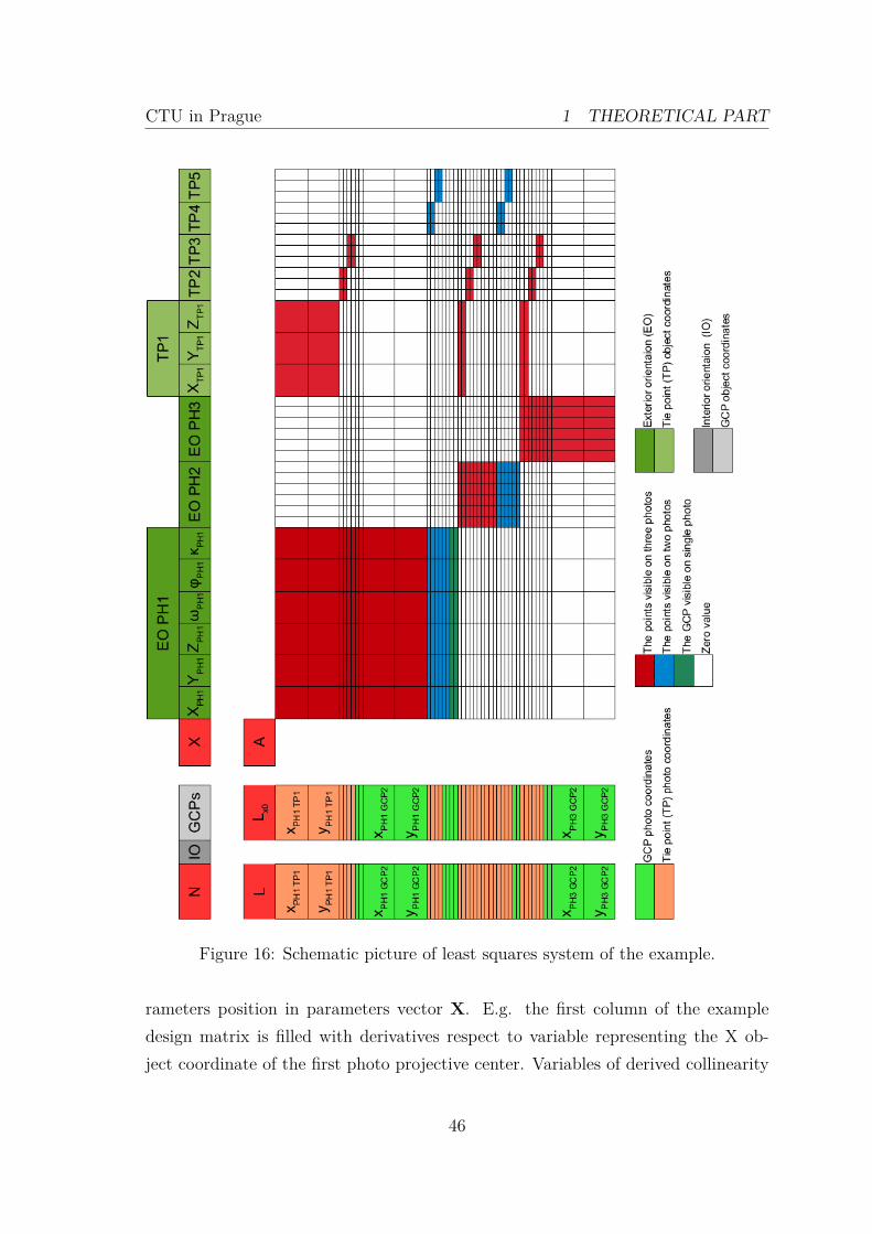
In the first least squares iteration, the initial values of adjusted parameters aregiven into parameters vector X representing tangent point of Taylor polynomialsand costs functions. The other non-adjusted parameters are given into N vector ofknowns. In the example, non-adjusted parameters are object coordinates of GCPsand interior orientation. Measured photo coordinates are given into vector of mea-surements L.
Design matrix A is calculated from derivatives of collinearity equations substi-tuting values from vectors X and N.
The vectors L and X give structure to design matrix A and vector LX0.
Order of partial derivatives of design matrix A is determined by adjusted pa-
45
CTU in Prague 1 THEORETICAL PART
Figure 16: Schematic picture of least squares system of the example.
rameters position in parameters vector X. E.g. the first column of the exampledesign matrix is filled with derivatives respect to variable representing the X ob-ject coordinate of the first photo projective center. Variables of derived collinearity
46
CTU in Prague 1 THEORETICAL PART
equations depends on the row. For instance, the first two rows represents partialderivative of collinearity functions including variables of the first point object co-ordinates and first photo exterior orientation. First row represents derivation of xcollinearity equation because in corresponding position of the measurements vectorL, there is x photo coordinate of the tie point 1. The second row of the designmatrix is composed of partial derivatives of y equation comprised of the same vari-ables. Variables of collinearity equation change in the other rows. For instance, thelast row corresponds to the y photo coordinate of the GCP 2 (see Figure 16). Thepartial derivation of the first column is equal to zero because the variable X of objectcoordinate of the first photo projective center was replaced by X of the third photoprojective center in collinearity equation. It should be noted that in the last row,there are no derivations respect to point object coordinates because the row repre-sents GCP. Object coordinates of GCPs do not belong to the adjusted parametersthus design matrix do not contain column representing partial derivatives respectto the GCP object coordinates.
Position in a vector LX0 is linked in the same way to a vector L as rows of designmatrix. Value of position is calculated by collinearity equations using correspondingvariables.
The relations nicely illustrates a pivot role of design matrix which links param-eters vector X with measurements vectors L and LX0.
If rows in design matrix A or positions L and LX0 are switched, as consequenceof the correspondence it is needed to switched them also in the other components.The same applies to columns of design matrix A and positions in parameters vectorX
The thesis does not deal in-depth with determination of weight matrix P. Sim-plest method is to represent it as identity matrix. More rigorous method is describedin 1.4.2.
All needed information is available to perform a first iteration of non linear leastsquare method (1.4.1). Refined values of vector X are obtained as result of aniteration. Another iteration can be performed by the same procedure with adjustedparameters vector X if termination criterion is not met (1.4.3).
47
CTU in Prague 1 THEORETICAL PART
1.8 Orthorectification
Orthorectification is a process transforming photo from perspective projection intoorthogonal projection (see Figure 5). There are two main methods for producingorthophoto. The first method is able to retrieve orthophoto from a single photo. Itrequires exterior, interior orientations of the photo and a shape of relief. Shape ofrelief is usually provided in a form of digital terrain model (DTM). DTM can begiven in the raster or vector form. Raster-based DTM describes relief with a uniformdensity defined by resolution of the raster. Vector-based DTM is comprised bycontinuous surface made of triangular irregular network (TIN). At the beginning oforthorectification, empty raster is allocated representing an orthophoto. It coversintersection of a photo scene and area of a DTM.
In the next step, the empty orthophoto is filled by values. All points repre-senting centers of pixels are given Z coordinates from DTM, then the points aretransformed into the photo coordinate system using collinearity equations. Becausea transformed point is represented by floating point, the value given to the cor-responding pixel in an orthophoto is determined by interpolation of surroundingpixels of the transformed point into a photo. Used interpolation methods, selectionof points for transformation etc. may vary, however, the main principle is still thesame. It is based on back projection of an object point into a photo to obtain valuesfor an orthophoto.
The other method can be considered as an extension of the first one because ini-tially it generates DTM then it recovers orthophoto according to the same principleas the first method. It is based on triangulation of object point from photo pointsrequiring interior and exterior orientation of photos to be known. The reconstructedpoint must be visible at least on two photos in order to solve the ray ambiguity. Itfollows that it requires more than one photo in contrast to the first method. Objectcoordinate system can be defined arbitrarily because there is no needed to definerelationship to the input DTM as the first method requires. Instead of this, DTM iscreated in arbitrary coordinate system directly by the method, hence orthophoto andDTM can be generated without any GCP. Approximate object points are calculatedby triangulation methods (1.6.4) then refined by the BBA.
The DTM is created from retrieved object coordinates. There are plenty of
48
CTU in Prague 1 THEORETICAL PART
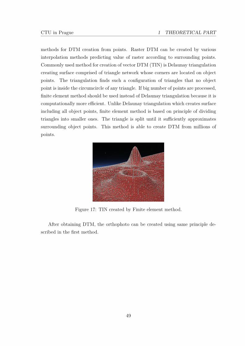
methods for DTM creation from points. Raster DTM can be created by variousinterpolation methods predicting value of raster according to surrounding points.Commonly used method for creation of vector DTM (TIN) is Delaunay triangulationcreating surface comprised of triangle network whose corners are located on objectpoints. The triangulation finds such a configuration of triangles that no objectpoint is inside the circumcircle of any triangle. If big number of points are processed,finite element method should be used instead of Delaunay triangulation because it iscomputationally more efficient. Unlike Delaunay triangulation which creates surfaceincluding all object points, finite element method is based on principle of dividingtriangles into smaller ones. The triangle is split until it sufficiently approximatessurrounding object points. This method is able to create DTM from millions ofpoints.
Figure 17: TIN created by Finite element method.
After obtaining DTM, the orthophoto can be created using same principle de-scribed in the first method.
49
CTU in Prague 2 ANALYTICAL PART
2 Analytical part
2.1 General solution of UAV bundle block adjustment
In 1990s Global Positioning System (GPS) become first globally operational nav-igation satellite system (GNSS). GPS allows to locate position of GPS unit withaccuracy ranging from millimeters to decimeters depending on used technique andother conditions. In photogrammetry, GPS is often employed with inertial mea-surement unit (IMU), which measures its orientations in a object space. The unitsgreatly simplifies obtaining of the initial values of exterior orientation in the pho-togrammetric aerial mapping missions. They provide all needed parameters of theexterior orientation with sufficient accuracy for performing of BBA. In order to beinformation useful, it is need to determine lever-arm offset describing shift of GPSunit to the perspective center and bore sight offset describing orientation of cameracoordinate system towards IMU coordinate system [27][p. 33]. These two quantitiesare determined in calibration process [27][p. 54]. The measured values from GPSand IMU units has to be corrected by the two quantities to represent true exteriororientation of a camera coordinate system. The quantities can be refined by BBAif collinearity equations are extended to include them.
Before operation of GPS, aerial photogrammetry had made some a priori assump-tions about a camera position, which simplified the collinearity equation in order toget the initial values of exterior orientation. For instance, it can be assumed that theaerial photo is vertical if orientation deviates from true vertical direction up to 2-3degrees. Applying the assumption to collinearity equations, they can be linearizedand approximate values can be computed easily from GCPs [26][p. 52].
Photogrammetric aerial mapping mission is prepared and carried out by expertsusing professional, properly calibrated equipment. As a consequence, cost of themissions is high. These facts prevents from further spreading of rigorous aerialphotogrammetry methods.
Nowadays, nearly everybody has camera in his or her pocket thus there is abig demand to provide very simple solution from the user point of view becausevast majority of the users have limited or no knowledge of photogrammetry andcomputer vision. Recent rise of civil UAV (see 1.3) sector has drastically reduced cost
50
CTU in Prague 2 ANALYTICAL PART
of mapping compared to rigorous aerial photogrametry mission employing mannedaircraft.
It follows the main requirement of the solution to be simple and cheap enoughin order to be adopted by ordinary users who do not want to spend money for otherdevices or to spend time studying complicated methods. Ordinary users just wantto take a group of a photos of a scene and get the job done by a software. Thefinal solution should be flexible to process both terrestrial and aerial photos givingorthophoto and structure/DTM as an output. No limitation on camera orientationshould be enforced because it should be capable of processing photos captured fromcamera held by hand or mounted on UAV. Due to instability of UAV flight trackand human hand, the photos must be considered as oblique.
In order to meet the requirement of simplicity, user should just need camera toobtain structure of the scene. Orthophoto creation would also need employment ofUAV in order to get images from approximately vertical point of view. No otherhardware device should be needed. All other steps should be done using free soft-ware, which can everybody freely share and use.
The solution should be flexible enough to process additional data known abouta scene, e.g. GCPs, positions of cameras etc. The additional data can increaseaccuracy of results and reduce computational time decreasing number of BBA it-erations needed for finding global minimum. It is very important for professionalphotogrammetric measurements where accuracy matters.
As a consequence of the general goals the minimum required input should bejust photos of the scene. It could be required to take photos of a calibration scene,however, it must be easy to construct it.
Another important requirement is to make whole process as much automatic aspossible, because if it would require a lot of time for an user to go through theprocessing chain, nobody would use it.
Following processing chain [14] should fulfill above mentioned requirements forthe solution:
• Camera calibration – determination of camera interior orientation. One groupof many techniques for calibration of the camera are based on processing ofphotos of 2D calibration patterns. Whole process is very simple from the
51

CTU in Prague 2 ANALYTICAL PART
user point of view. It is needed to print the pattern on sheet of paper andtake photos of the pattern from different positions. The calibration is doneautomatically. No additional user input except a photos of a pattern is needed.
• Tie point identification – it can be done fully automatically by pattern match-ing algorithms.
• Retrieval of initial values for BBA – it is fully automatic process without needof any manual user input. As input it needs tie points and interior orientationof camera given by previous two steps. Optional step of transformation intoworld coordinate system needs users assistance to provide GCPs [12] in themost cases.
• Bundle block adjustment (BBA) – it is fully automatic integrating informationfrom all three previous steps.
2.1.1 Camera calibration
Camera calibration is a process dealing with determination of the interior orien-tation parameters including distortion. Several methods can be used for cameracalibration [43]. One group of calibration methods are based on photos capturingcalibration object covered with calibration points. Relative position of the points toeach other is precisely determined.
The methods can be further divided according to dimension of a calibrationobject:
• 3D reference object based calibration – It allows to reach very good accuracy ofdetermined interior orientation parameters. One type of the common calibra-tion objects is comprised of three or two perpendicular planes covered by thecalibration points. Drawback of 3D calibration is that accurate constructionof the calibration object is difficult.
• 2D plane based calibration – It is less accurate compared to 3D calibration.The accuracy can be improved by taking more photos of a calibration object.On the other hand calibration object can be printed on a sheet of paper, whichis much easier compared to construction of a 3D calibration object.
52
CTU in Prague 2 ANALYTICAL PART
Another method is a self-calibration, which finds values of the interior orientationparameters by BBA. However, at least initial values of focal length and principalpoint must be known. Usually focal length and chip size are publicly availableby manufacturer. The principal point can be computed dividing chip size by two,because it is supposed that it lies close to the middle of the photo. It is moreconvenient to use pixels as units of the interior orientation, therefore focal length andprincipal point coordinates can be converted from millimeters units into pixels usingphoto resolution. Interior orientation based on manufacturer information should notbe interpreted as very accurate therefore it has to be refined by camera calibrationprocess. Including interior orientation as parameters of BBA can lead into over-parametrization which may lead to deterioration of resulting accuracy. In the caseof self-calibration it is recommended to take convergent photos from many differentdirections and positions in order to avoid correlation of adjusted parameters.
In order to keep interior orientation parameters stable, the camera during takingphotos of a scene should have fixed same zoom level, because interior orientationparameters are very sensitive to zoom changes [13]. Influence of focus change is lesssignificant than zoom influence. It affects the parameters if a camera is in shortdistance from a scene. Also change of a resolution may affect interior orientationparameters, which mostly depends on specific camera type. Change of other camerafeatures as exposure time or aperture do not have so significant effect on interiororientation.
2.1.2 Tie points identification
From a developer point of view, the simplest way of tie points identification is to forceuser to locate tie points on the photos manually. However, the user would have towaste a lot of time on such a dull task. Luckily, there are algorithms able to identifytie points on photos automatically. The state of the art algorithms are SIFT [40]and SURF [41]. The algorithms allows to identify tie points in corresponding photoscapturing same parts of a scene without need to provide any other information.Unfortunately, both algorithms are patented in USA therefore their use should beavoided in open source community.
Recently new BRISK [15] and FREAK [1] algorithms have been developed. The
53
CTU in Prague 2 ANALYTICAL PART
algorithms do not posses a patent restriction.
Another issue of tie points matching is determination of the corresponding pho-tos. If photos are taken in a strip, it is easy because the corresponding photos arecomprised from neighborhood photos in a strip. If there is no a priori informationabout photo order, the easiest way is to use brute force checking all photo pairscombinations to find correspondence. If higher number of photos needs to be pro-cessed, it become unsolvable problem because of big number of combination to bechecked. In order to make it more efficient, a visibility map [2] can be build up. Thevisibility map is a graph where nodes represent photos. The graph edges connectsphotos if there is correspondence between them. It is possible to use informationfrom GPS and IMU units for creation of the visibility map.
Further speed up can be achieved by decreasing of photos resolution for firstsearch of tie points. The first search only identifies correspondence of photos. Insecond search, tie points extraction is performed on full resolution on photo pairswith identified correspondence from the previous step.
2.1.3 Retrieving initial values for bundle block adjustment
The next step is to utilize all known information (interior orientation and extractedphoto coordinates of tie points) to get missing initial values of parameters for BBA.
Collinearity equations (26) are the cost functions of BBA thus only missinginformation to calculate them are parameters of exterior orientation and objectcoordinates of tie points because parameters of interior orientation are obtained bya camera calibration procedure (see 2.1.1).
Many methods deal with obtaining of initial values of the exterior orientation.They differ in information which they require for input, computation time and ac-curacy. In order to fulfill the set up requirements chosen method should be ableto retrieve exterior orientation using just photo coordinates of tie points and inte-rior orientation of camera. The method should be general in terms of capability toprocess oblique photos and robustness to various object points configuration.
Methods can be divided into following groups according required information:
• Methods requiring knowledge of the object point coordinates to retrieve exte-
54
CTU in Prague 2 ANALYTICAL PART
rior orientation. The requirement would have negative impact on processingchain because it would require manual identification of the object coordinates,thus this group of methods should be avoided.
• Group of methods based on making assumption about the configuration ofcameras (e.g. see 2.1).
• Methods based on epipolar geometry (1.6.3) using essential matrix propertiesto retrieve relative orientation. The epipolar methods are closed form com-puter vision algorithms able to determine relative orientation (essential ma-trix) from photo coordinates of tie points coordinates normalized by cameracalibration matrix.
In order to meet set up requirements noted in 2.1, the group of epipolar algo-rithms seems to be the best choice. Unlike the second group of algorithms, theyare general to be capable of processing oblique photos. Unlike to the first group ofmethods, the epipolar algorithms do not require a priori information about objectpoint coordinates.
Individual epipolar algorithms are called according to required number of iden-tified tie points in two photos. Thus eight, seven, six and five point algorithmsbelongs the the group. The five point algorithm seems to perform best in the mostcases [33] and it is not sensitive on planar points configuration as the others.
Only one case, when the five point algorithm [22] underperforms [4] the others isforward motion of the camera. This flaw can be eliminated by joint usage of eightand five point algorithms.
Main disadvantage of the five point algorithm is that it can produce up to tensolution. Hence it is needed to asses the solutions and select the correct one. Thenumber of solutions can be reduced by assumption that all tie points lies in front ofboth photo planes. After sorting out obviously non sense solution, the correct solu-tion can be found by assumption that it gives minimum sum of epipolar distances.Epipolar distance is photo point distance from epipolar line. The epipolar line iscomputed from corresponding photo point in another photo using fundamental ma-trix.
Because matching algorithms are not perfect, certain number of the tie points are
55
CTU in Prague 2 ANALYTICAL PART
matched incorrectly therefore it is needed to be relative orientation robust enoughto deal with the outliers.
The RANSAC [39] method is commonly used with the epipolar algorithms tomake it more robust for effect of the outliers. Principle of RANSAC is based onfinding such a solution in group of measurements containing outliers which wellapproximates inliers.
In the group of epipolar algorithms, RANSAC selects random tie points in everyiteration. The number of selected tie points is chosen according to minimum numberwhich the epipolar algorithm requires. The epipolar algorithm is launched withthe selected points as an input, giving essential matrix as output. Quality of theessential matrix is assessed by calculation of epipolar distances of tie points. It isspecified some threshold of the distance used for decision whether the measurementis inlier or outlier. Another threshold specifies minimum percentage of inliers fromall tested points. If percentage of inliers is higher than in any previous iteration andit satisfies the minimum percentage of inliers threshold, then the essential matrixis set as the best fitting and iteration continues. The iteration terminates afterreaching maximum number of iterations returning the best fitting essential matrix.
After essential matrices are obtained, all needed information for calculation ofinitial object point coordinates is available. The object points coordinates can becomputed by triangulation methods described in 1.6.4.
2.1.4 Common relative coordinate system
All approximate values needed for calculation of BBA collinearity cost functions areavailable. However, it is not possible to adjust scene in one bundle, because objectcoordinates of tie points and exterior orientations are given in individual objectcoordinate systems of relative orientations of photo pairs.
Therefore it is needed to transform all features from the individual systems into acommon relative coordinate system by subsequent transformation described in 1.6.6.
56
CTU in Prague 2 ANALYTICAL PART
2.1.5 Transformation into world coordinate system
The difference between a world coordinate system and common relative system isthat the common one is defined by arbitrary selected relative orientation. World co-ordinate system definition is standardized. Thanks to the standardized definition, itis connected to all other commonly used world systems through defined transforma-tions to these systems. GCP object coordinate are usually expressed in some worldcoordinate system. In order to be information of precise GCP coordinates usablein BBA, it is needed to transform common relative system into the world systemof GCPs. When the scene is transformed into world coordinate system, it can alsobe combined with other data e.g. maps which are expressed in some world coordi-nate systems. Moreover availability of precisely determined GCP can significantlyimprove results of BBA.
The transformation is called Helmert transformation. It is comprises from threemain steps: rotation, scaling and translation (see 1.6.7).
In order to make transformation of the common system into the world coordinatesystem possible, it is needed to have at least 3 GCPs, with known initial coordinatesin the common relative system. This step is optional because BBA can be performedalso in the common coordinate system.
2.1.6 Bundle block adjustment
All initial values of parameters in collinear equations (26) are obtained and trans-formed into common coordinate system, thus BBA can be performed.
The main reason for employing BBA is to improve accuracy of results. In orderto obtain initial values it is merely used information from relative orientation ofphoto pairs. However, the object points are usually visible from more than two pho-tos. This redundancy is not fully taken into account during retrieval of initial valuesbecause object points are calculated just from two photos ignoring additional infor-mation from another photos where the point was also identified. Only non-rigorousredundancy in relative orientation process is that the same object point can be cal-culated from multiple photo pairs of relative orientations. Single object coordinatesof the point can be calculated after transformation into a common system.
57
CTU in Prague 2 ANALYTICAL PART
Unlike initial values retrieval, BBA utilizes redundancy rigorously therefore itcan significantly improve accuracy of the adjusted parameters. Usually, the initialvalues of parameters contains certain amount of outliers caused by instabilities ofprevious steps of the processing chain. The BBA can also significantly improveaccuracy of the few evidently wrongly determined parameters. Moreover, if a photopoint is wrongly identified in a photo, such a point can be recognized and its negativeeffect can be eliminated.
If at least three GCPs are known, the scene can be transformed into worldcoordinate system thus ordinary non-linear least square method (1.4.1) can be used.Otherwise, it is needed to use free network least squares (1.4.4) to cope with datumdeficiency.
2.2 GRASS GIS orthorectification workflow
GRASS (1.2) belongs among few open source GIS software supporting orthorectifi-cation [29].Orthorectification is performed by i.ortho.photo [18], [21][p.253 - p.267]module. The module is comprised of submodules representing individual steps ofGRASS orthorectification workflow.
The module was developed in 1990s, when analog photos were mostly processed.Therefore it supports transformation of a scanned image of an analog photo fromcoordinate system of the scanned image into the photo coordinate system using fidu-cial marks. The marks are used for calculation of affine transformation coefficientsfrom known photo coordinates and corresponding scanned image points. It is doneby i.photo.2image submodule allowing to identify the fiducial marks in scanned im-age coordinates system and assign their known photo coordinates. If digital photosare processed, imaginary fiducial marks have to be defined which can be located e.g.in the middle of photo sides.
The interior orientation parameters of camera are supposed to be known and canbe managed by i.photo.camera submodule. The data model is not taking distortioncoefficients into account. The next step is retrieval of the exterior orientation param-eters by i.photo.2target submodule. The retrieval of exterior orientation is based onnon-linear least squares iteration. Unlike BBA, the photos are adjusted separatelytherefore only GCPs can be used because it is not possible to determine object coor-
58
CTU in Prague 2 ANALYTICAL PART
dinates of tie point from single photo. At least three ground control points (GCPs)has to be available since six exterior parameters are determined. Three availableGCPs are just theoretical minimum. In practice, it is needed to provide at least12 GCPs to get reasonably accurate results. Exterior orientation can be includedinto input using i.photo.init submodule in order to be used as initial values for leastsquares iteration. Otherwise, it is supposed that images are vertical therefore twoof three rotation angles are set to 0 and the last angle is computed as difference ofGCPs centroid slope in photo coordinate system to the slope in object coordinatesystem taking into account only X, Y coordinates in both system. Projective centerobject coordinates are given equal to the centroid coordinates.
As the last step, the orthorectified photo is computed by i.ortho.rectify submod-ule. GRASS uses single photo orthorectification method (see 1.8) requiring knownDTM in order to deal with elevation differences.
The main disadvantages of GRASS orthorectification processing chain are:
• It orthorectifies photos separately thus, unlike BBA, it ignores significant partof information which can greatly improve accuracy and robustness of a finalorthophoto.
• Because of single photo orthorectification method, it is necessary to have DTMof a scene in order to generate an orthophoto. Precise high resolution DTM isnot usually available for free thus the requirement can be obstacle preventingfrom creation of accurate orthophoto. If sufficiently precise DTM is not avail-able freely available DTM with usually lower resolution can be used. However,accuracy of final orthophoto will be limited by insufficient resolution of DTM.
• The requirement for at least three visible GCPs from every photo can besometimes also difficult to meet. Close range flight of UAV can easily takehundreds of photos. It is nearly impossible to measure enough GCPs for allphotos because one photo covers tens of meters of terrain in such a case. Onthe other hand, the reproach is not valid in context of the current GRASSworkflow because it requires DTM, which allows to obtain enough GCPs.
• Moreover the workflow does not contain any submodule for retrieval of initialexterior orientation except the case of the vertical photo. If the photo is not
59
CTU in Prague 2 ANALYTICAL PART
vertical, it is needed to know at least approximate exterior orientation in orderto the least squares iterate towards global minimum.
The disadvantages are big obstacle making current implementation of orthorec-tification difficult to use for processing of UAV or terrestrially taken oblique photosoften lacking both GCP and DTM information. However, the current GRASS or-thorectification workflow can be successfully used for processing of aerial photosfrom photogrammetric missions.
Currently i.ortho.photo module works in stable version of GRASS (6.4.3). De-velopment version of GRASS (7) does not fully support all orthorectification fea-tures as a consequence of rendering architecture change. Hence, new front end ofthe orthorectification has to be developed in order to make it fully operational inGRASS 7.
60
CTU in Prague 3 IMPLEMENTATION
3 Implementation
3.1 Used technologies
3.1.1 OpenCV
OpenCV2 is an open source computer vision and machine learning library releasedunder free BSD license. The library contains thousands of algorithms mainly focusedon real time image processing. Originally, it was developed by Intel. Currently,OpenCV is supported by non-profit organization OpenCV.org.
The library is written in C++ programming language including interfaces toother programming languages as C, Python, Java etc.
OpenCV library contains very useful algorithms dealing with retrieval of struc-ture from group of photos. It includes algorithms for determination of relativeorientation and object coordinates of the tie points. Recently, implementation offive point algorithm has been included into development version of OpenCV. An-other relevant group of algorithms deals with camera calibration. OpenCV cameracalibration is based on 2D plane based calibration. There are also implementedfeature matching algorithms used for tie points identification.
3.1.2 Python
Python is a programming language developed since 1991. Its code is easily readableand comprehensible therefore it is often picked as first programming language tolearn. Python is employed in wide range of software from simple scripts to complexsystems. It is high level programming language compared to languages as C++or C hence the development process is usually significantly faster. On the otherhand, Python is significantly (hundred times) slower compared to C++. Despitethe slowness, Python is usually more preferred over C++/C thanks to its flexibilityand simplicity. It is used as top level glue in many application, where it takes careabout the main workflow. The parts of application doing heavy computation can bewritten in other faster programming languages and called from Python code. This is
2http://opencv.org
61
CTU in Prague 3 IMPLEMENTATION
very powerful combination which allows to speed up development process preservingspeed of application.
Thanks to its popularity, the Python world is very rich. Thousands of Pythonopen source libraries make life of programmer much easier. Even if library is notimplemented in Python, it is possible to automatically generate Pythonic interfaceby some of available open source tools (e.g. SWIG). And even if the library doesnot have Python interface it is possible to use the tools as e.g. ctypes or Cython tocall libraries functions directly from Python.
NumPy NumPy is free software Python library supporting multidimensional ar-rays and many array operations including linear algebra operations. Killer featureof NumPy is its speed. It allows to write very effective code with just a few lines.Many NumPy operations can be also rewritten by Python code using for loops. IfNumPy function is called, the difference is that computation is perform by highlyoptimized C code. It causes much faster performance compared to Python codeespecially if arrays contain a lot of elements. Sometimes, it is difficult for NumPybeginner to figure out the way how to write problem avoiding loops. However, asthe user gets experienced it become easy to do it.
NumPy is so widely used Python library that it has become one of fundamentallibraries thus many other libraries and applications rely on NumPy requiring itsinstallation in order to work.
SimPy SimPy is another free software Python library focused on process-baseddiscrete-event simulation. Among many other features it supports symbolic expres-sion. The expressions can be useful e.g. for computation of a derivation of a function.A result of a derivation is a symbolic expression. The symbolic expression can beused as function for calculation of numeric values of a derivation.
SimPy is used for generation of partial derivatives of collinearity equation fordesign matrix of BBA. Thanks to it, it is easy to add new parameters into collinearityequations as e.g a distortion coefficients or a leverage arm offset, because it is justneeded to extend collinearity equations and the source code of partial derivatives isgenerated automatically by the library.
62
CTU in Prague 3 IMPLEMENTATION
3.1.3 GRASS programming environment
Architecture of GRASS (1.2) is composed of core libraries and modules. There isgeneral GIS library dealing with basic setup of GRASS environment. It includesmanagement of GRASS variables and environment variables. These variables arevery important because GRASS is not one monolithic software but it is composed ofmany small software packages called modules. When a module is launched, essentialinformation about GRASS session (current location, mapset etc.) is passed throughthe variables. Another core libraries are dealing with different GIS data e.g. raster,vector or imagery library etc. All core libraries are written in C.
In the recent years, GRASS support of Python programming language has beensignificantly improved. The main motivation has been to make development ofGRASS accessible for wider base of developers because Python is very simple andpopular programming language. In many cases, using C programming language isoverkill for development of a module which cost developer much more time with nosignificant gains compared to writing it in Python. Nowadays, Python is supportedvery well in GRASS. Functions of the C libraries can be accessed from Pythonthrough ctypes interface being automatically generated during compilation for allGRASS libraries. Another option, how to call C functionality from Python, isPyGRASS API taking full advantage of Python beauty. The last option is callingmodules from Python. Unlike libraries, GRASS module layer is more abstract there-fore some specific functionality may be missing compared to the libraries. On theother hand, some functionality is implemented only in module layer therefore thelast option is only one possibility how to access the functionality. Calling modulecompared to calling library function is slower. Big momentum of Python integrationinto GRASS has been given by development of wxPython graphical user interface.Thanks to the Python support, GRASS has attracted new developers who has im-plemented many new modules.
3.2 Modification of GRASS GIS orthorectification workflow
The implementation should fulfill these goals:
• Backward compatibility preserving current implementation of orthorectifica-
63
CTU in Prague 3 IMPLEMENTATION
tion. It has proved its qualities in processing of photos from rigorous aerialphotogrammetric missions.
• Take advantage of modularity of i.ortho.photo module. If the workflow iscomprised of modules/submodules with clearly defined interface, it is possibleto implement several different algorithms for every step of orthorectification.The main advantage of this approach is that workflow can be adapted tospecific needs allowing to use the most suitable algorithms to achieve maximumaccuracy.
• Another more abstract module should be created to be used by less advancedusers who do not have sufficient knowledge to create individual workflow. Thesimplicity would be the main concern of the module. User should be ablejust throw in some photos and get the results done (e.g. DTM, structure ororthophoto) automatically. The module would employ the lower lever modules.Furthermore, it would include intelligent system adapting to individual datasetneeds achieving as good accuracy as possible. The system should substituteknowledge of an experienced user in order to assemble workflow on the fly.
• Eventually, a graphical user interface should be developed. The interfaceshould allow to identify tie points and ground control points, visualize theresults and help with assessment of accuracy.
If all the goals were fulfilled, GRASS would become unique, flexible, state of theart orthorectification software available for free! It could be used by wide spectrumof users from amateurs to experts. Due to time limitation, the thesis deals onlywith basic implementation of the functionality of some of the lowest level modules.However, it is very important to have the ultimate goal in mind to properly designthe solution from initial steps in order to save time spend on refactoring in futuredue to bad design. Moreover, seeing the big picture allows to focus on crucial partsof whole processing chain.
In order to meet the implementation requirements, the whole processing chaincan be implemented in form of following GRASS low level modules:
• Camera calibration module – retrieves interior orientation supposed to beknown by next steps of the workflow.
64
CTU in Prague 3 IMPLEMENTATION
• Point match module – identification of tie points in photos.
• Initial values module – computes initial values of exterior orientation andobject coordinates of tie points, which are used in BBA. It uses informationfrom the both previously mentioned modules.
• BBA module – performs BBA based on data obtained by the other modules.The module gives refined parameters as output (e.g. adjusted exterior orien-tation and object points coordinates).
Object point coordinates can be used for generation of DTM since the workflowretrieves them. It can be taken advantage of rich GRASS environment includingplenty of modules for interpolation raster DTM from points. Also it can be createdvector DTM using e.g. v.voronoi module. The obtained DTM, exterior orientationsand interior orientations can be used as input into i.ortho.rectify submodule forgeneration of an orthophoto .
3.2.1 Camera calibration module - i.ortho.cam.calibrate
The calibration module i.ortho.cam.calibrate is a simple module written in Python.It calls function from OpenCV calib3d module. The module is based on calibrationfrom 2D pattern, which can be easily printed. The most important input parameterdefines directory with photos capturing 2D pattern taken by a calibrated camera.In order to obtain good results of camera calibration, at least 10 convergent imagesfrom different positions all around the pattern should be taken [24].
OpenCV is able to work with following calibration patterns:
• chessboard pattern,
• asymmetric pattern of circles,
• symmetric pattern of circles.
Generally speaking, the circle patterns achieves higher accuracy [24].
The identification of pattern points (centers of circles or corners of chessboardsquares) are done by OpenCV functions which are able to identify the points without
65

CTU in Prague 3 IMPLEMENTATION
any other additional information except number of circles or squares per row andcolumn of a captured pattern then the points coordinates are refined to achievesubpixel accuracy.
Besides captured photos and the number of rows and columns in the pattern noother information is needed to retrieve interior orientation of a camera. Object co-ordinates are defined arbitrary by the module according to pattern type and numberof rows and columns of pattern marks.
During calibration, initial exterior orientation of photos and interior orientationof camera are retrieved by closed form solution exploiting condition that all pointsare on a plane. First guess of interior orientation is calculated ignoring distortion.In the next step, initial values of distortion parameters are calculated by linearleast squares method where all parameters except a distortion parameters are keptfixed. In the last step, iterative BBA adjusting all interior orientation and exteriororientation parameters is performed. The method is in-depth described in [42].
The computed interior orientation is saved into GRASS camera file to be usedby other GRASS orthorectification modules. The module modifies camera file viai.ortho.camera module (GRASS 7 equivalent to i.photo.camera in GRASS 6). TheGRASS camera data model was extended to support radial and tangential distortioncoefficients. A distortion has serious effect especially in cheap cameras, due toimperfections of their optical system.
3.2.2 Bundle block adjustment data model
The initial values module and the BBA module basically handles same data, thusthe data model can be designed in the similar way. Three common classes can beidentified to be shared by both modules:
• Camera – the class stores information about interior orientation parametersincluding distortion. Camera class contains references to the photos classestaken by the camera.
• Photo – members of photo class are references to the points identified on thephoto and camera which took the photo.
66
CTU in Prague 3 IMPLEMENTATION
• Point – the class denotes representation of same object point in different photos(tie points). If the point is GCP it includes also information about its objectcoordinates.
The classes sufficiently express a structure together with relations of an elementsof a structure. They offer enough flexibility for adaptation to needs of both modulesby subclassing. For instance, the initial module requires to store more object coor-dinates of same point since the coordinates may by calculated from more relativeorientations. The chosen data model allows to create child class of the abstractPoint class with members storing all the coordinates.
It must be noted that the implementation submitted with the thesis containsfunctionality of both modules implemented in single i.ortho.bba module. It does notmatter in the current stage of prototype, however, in the future, it should be splitinto two modules in order to fulfill implementation goals.
3.2.3 Initial values module - i.ortho.initial
The i.ortho.initial module retrieves initial values of photos exterior orientations andinitial object coordinates of tie points. If at least 3 GCPs are available in an input,relative coordinate system is transformed into world coordinate system of the GCPby applying Helmert transformation (1.6.7).
The module input is:
• interior orientations of cameras e.g. computed by i.ortho.cam.calibrate,
• photo coordinates of tie points.
Because the exterior orientation is defined by relative coordinate system of thetwo cameras, it is needed to be transformed into a common relative coordinatesystem defined by the reference pair.
The module builds internally graph-like structure where nodes represent photosand edges hold information about number of corresponding tie points identified onboth photos linked by an edge. Relative orientation of photo pairs is subsequentlyperformed in order defined by going through the graph. Photo pair with the highestnumber of corresponding tie points is selected as reference pair. The pair defines
67
CTU in Prague 3 IMPLEMENTATION
common relative system thus its relative orientation is calculated as the first. Everyother relative orientation system is transformed to the common system by processof transformation of relative orientations (1.6.6). The next photo pair for transfor-mation is chosen from subset of edges connecting nodes where one photo is alreadytransformed into common system while another one is not. The chosen pair be-longs to an edge from the subset representing the highest number of correspondingtie points among all edges in the subset. Relative orientation of the chosen pair isperformed by the five point algorithm. It has been recently added into developmentversion of OpenCV as a function findEssentialMat. The algorithm returns essen-tial matrix (see 1.6.3). Exterior orientation is retrieved (1.6.5) from the essentialmatrix by recoverPose function. When relative orientation is known, photo coor-dinates of tie points visible from both photos of pair are refined by correctMatches
function based on optimal solution (1.6.4). After that, the refined photo coordinatesare used for calculation of object coordinates by triangulatePoints function usingDLT method described in 1.6.4. As a last step object points and relative orientationare transformed into common system. The procedure is repeated until the subset ofedges is not empty. Manual of all OpenCV functions is available in [23].
The last step of the module is transformation of the relative coordinate systeminto a word coordinate system. Helmert transformation coefficients are retrieved bycode from v.rectify module [16] using the closed form method 1.6.7, This moduleis used e.g. for transformation of Lidar point clouds from an arbitrary coordinatesystem into a world coordinate system. Part of v.rectify code calculating Helmerttransformation coefficients was moved from the module into the GRASS ImageryLibrary in order to be accessible also by other modules. The i.ortho.initial moduleuses ctypes interface to call it. Calculated Helmert transformation coefficients areapplied on the exterior orientations of cameras and object coordinates of the tiepoints. The transformation is performed only if at least three GCP are available.
The output of the module are exterior orientations and object coordinates incommon relative or world coordinate system.
68
CTU in Prague 3 IMPLEMENTATION
3.2.4 Bundle block adjustment module - i.ortho.bba
The BBA module performs non-linear least squares iteration, which uses collinearityequations as the cost functions. The module input represents all parameters ofcollinearity equations:
• tie points photo coordinates – e.g. identified manually or automatically bypoints matching algorithms,
• interior orientations of cameras – e.g. computed by i.cam.calibrate,
• exterior orientations of cameras – e.g. initial values can be computed byi.ortho.initial,
• tie points object photo coordinates – e.g. initial values can be computed byi.ortho.initial.
The module performs non-linear least square iteration until correction of theparameters are smaller than defined threshold. The module is able to perform non-linear least squares as free network (1.4.4). Another option is to use at least threeGCPs as knowns and thus solve it in classical way as described in 1.4.1.
The output of the module is the adjustment protocol. In the protocol, thereis described every iteration of the BBA including correction for all adjusted pa-rameters and standard deviations computed from covariance matrix calculated fromadjustment.
69

CTU in Prague 4 TEST CASE
4 Test case
The processing chain has been developed and tested on data kindly provided byMartin Řehák. The photos from testing data capture following scene:
The available information about scene includes:
• points identified on the photos (approx. 1000 representing 64 object points),
• position of photos (45) (lever arm offset + object coordinates from GPS unit),
• GCPs (7),
• interior orientation of a camera capturing all photos of the scene. The camerais first generation of Sony NEX-5 with ultra wide pancake 16 mm lens. Widthof the captured photos was 4592 and height 3056 pixels. The camera containsimage sensor has approximate size 25.1 × 16.7 mm.
Every parameter includes its standard deviation.
Figure 18: Scene of the test case.
70
CTU in Prague 4 TEST CASE
The data contains also protocol of processing done by Bingo-F software [9] re-vealing information about steps performed by the software to retrieve structure ofthe scene. Information from the protocol was very helpful for me because it gaveme first hint about the steps of the processing chain.
Bingo-F is widely used by photogrammetric experts. During its existence, it hasproved its qualities on various scenes configurations. It is miles ahead comparedto the developed processing chain in the thesis therefore the results of the Bingo-Fadjustment were regarded as reference for obtained data.
Generally, Bingo-F processing chain is very similar to the developed one, de-scribed in-depth in the previous chapters. The first step is relative orientation ofpairs then the pairs are transformed into common relative coordinates system. Afterthat, Helmert transformation is performed into world coordinate system. BBA isperformed as the last step.
Unlike the developed processing chain, the Bingo-F software takes into accountinformation about position of cameras included in the data. Because the developedprocessing chain should be general as much as possible, it was decided that thefirst version would ignore this information. According to the set up goals, the finalsolution should require only photo coordinates of tie points and interior orientationof cameras. In the future, it is possible to extend the processing chain to work withadditional information to improve accuracy of the results.
The Bingo-F processing chain is very robust, capable of identification and rulingout of blunders in individual steps of its processing chain.
Bingo-F protocols reveals following information about performed steps:
• Relative orientation – it is not possible to find out algorithm used for calcula-tion of relative orientation.
• Transformation to common relative system – Bingo-F performs so called "Pre-adjustment" of some points. It is probably some type of free network BBA.Also during computation of scale, blunder check is preformed inspecting adifferences between the object coordinates of points used for computation ofscale. The difference is calculated between point in common relative systemand correspondent point determined from relative orientation pair after trans-formation into the common system. If standard deviation of the differences
71
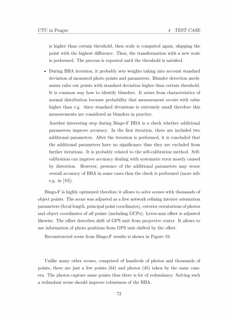
CTU in Prague 4 TEST CASE
is higher than certain threshold, then scale is computed again, skipping thepoint with the highest difference. Then, the transformation with a new scaleis performed. The process is repeated until the threshold is satisfied.
• During BBA iteration, it probably sets weights taking into account standarddeviation of measured photo points and parameters. Blunder detection mech-anism rules out points with standard deviation higher than certain threshold.It is common way how to identify blunders. It arises from characteristics ofnormal distribution because probability that measurement occurs with valuehigher than e.g. three standard deviations is extremely small therefore thismeasurements are considered as blunders in practice.
Another interesting step during Bingo-F BBA is a check whether additionalparameters improve accuracy. In the first iteration, there are included twoadditional parameters. After the iteration is performed, it is concluded thatthe additional parameters have no significance thus they are excluded fromfurther iterations. It is probably related to the self-calibration method. Self-calibration can improve accuracy dealing with systematic error mostly causedby distortion. However, presence of the additional parameters may worseoverall accuracy of BBA in some cases thus the check is performed (more infoe.g. in [10]).
Bingo-F is highly optimized therefore it allows to solve scenes with thousands ofobject points. The scene was adjusted as a free network refining interior orientationparameters (focal length, principal point coordinates), exterior orientations of photosand object coordinates of all points (including GCPs). Lever-arm offset is adjustedlikewise. The offset describes shift of GPS unit from projective center. It allows touse information of photo positions from GPS unit shifted by the offset.
Reconstructed scene from Bingo-F results is shown in Figure 19.
Unlike many other scenes, comprised of hundreds of photos and thousands ofpoints, there are just a few points (64) and photos (45) taken by the same cam-era. The photos capture same points thus there is lot of redundancy. Solving sucha redundant scene should improve robustness of the BBA.
72
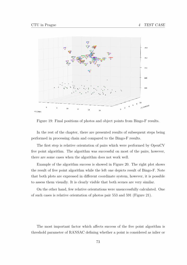
CTU in Prague 4 TEST CASE
Figure 19: Final positions of photos and object points from Bingo-F results.
In the rest of the chapter, there are presented results of subsequent steps beingperformed in processing chain and compared to the Bingo-F results.
The first step is relative orientation of pairs which were performed by OpenCVfive point algorithm. The algorithm was successful on most of the pairs, however,there are some cases when the algorithm does not work well.
Example of the algorithm success is showed in Figure 20. The right plot showsthe result of five point algorithm while the left one depicts result of Bingo-F. Notethat both plots are expressed in different coordinate system, however, it is possibleto assess them visually. It is clearly visible that both scenes are very similar.
On the other hand, few relative orientations were unsuccessfully calculated. Oneof such cases is relative orientation of photos pair 553 and 591 (Figure 21).
The most important factor which affects success of the five point algorithm isthreshold parameter of RANSAC defining whether a point is considered as inlier or
73
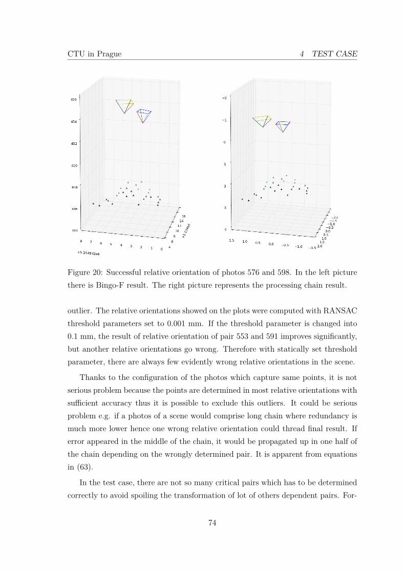
CTU in Prague 4 TEST CASE
Figure 20: Successful relative orientation of photos 576 and 598. In the left picturethere is Bingo-F result. The right picture represents the processing chain result.
outlier. The relative orientations showed on the plots were computed with RANSACthreshold parameters set to 0.001 mm. If the threshold parameter is changed into0.1 mm, the result of relative orientation of pair 553 and 591 improves significantly,but another relative orientations go wrong. Therefore with statically set thresholdparameter, there are always few evidently wrong relative orientations in the scene.
Thanks to the configuration of the photos which capture same points, it is notserious problem because the points are determined in most relative orientations withsufficient accuracy thus it is possible to exclude this outliers. It could be seriousproblem e.g. if a photos of a scene would comprise long chain where redundancy ismuch more lower hence one wrong relative orientation could thread final result. Iferror appeared in the middle of the chain, it would be propagated up in one half ofthe chain depending on the wrongly determined pair. It is apparent from equationsin (63).
In the test case, there are not so many critical pairs which has to be determinedcorrectly to avoid spoiling the transformation of lot of others dependent pairs. For-
74

CTU in Prague 4 TEST CASE
Figure 21: Unsuccessful relative orientation of photos 553 and 591. In the leftpicture there is Bingo-F result. The right picture represents the processing chainresult.
tunately, the reference pair defining common relative system is very stable as wellas the other core pairs with a lot of depending pairs. Probably, there is some cor-relation between tie point number and success rate of RANSAC loop in selection ofcorrect solution. Therefore, another way how to improve stability of the solutioncould be identification of more tie points. It could be done automatically by patternmatching algorithms. In the test case, there are 27 tie points in the reference pairgradually decreasing 6 points in the pair merged as last.
During the transformation process, all object coordinates representing the samepoint computed from different relative orientations are transformed into the com-mon relative system individually. Then, the final coordinates of object points aredetermined as median of the corresponding coordinates in common system. Median
75
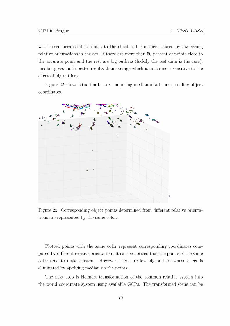
CTU in Prague 4 TEST CASE
was chosen because it is robust to the effect of big outliers caused by few wrongrelative orientations in the set. If there are more than 50 percent of points close tothe accurate point and the rest are big outliers (luckily the test data is the case),median gives much better results than average which is much more sensitive to theeffect of big outliers.
Figure 22 shows situation before computing median of all corresponding objectcoordinates.
Figure 22: Corresponding object points determined from different relative orienta-tions are represented by the same color.
Plotted points with the same color represent corresponding coordinates com-puted by different relative orientation. It can be noticed that the points of the samecolor tend to make clusters. However, there are few big outliers whose effect iseliminated by applying median on the points.
The next step is Helmert transformation of the common relative system intothe world coordinate system using available GCPs. The transformed scene can be
76
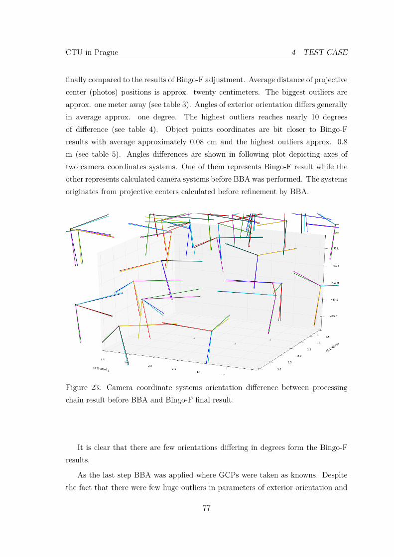
CTU in Prague 4 TEST CASE
finally compared to the results of Bingo-F adjustment. Average distance of projectivecenter (photos) positions is approx. twenty centimeters. The biggest outliers areapprox. one meter away (see table 3). Angles of exterior orientation differs generallyin average approx. one degree. The highest outliers reaches nearly 10 degreesof difference (see table 4). Object points coordinates are bit closer to Bingo-Fresults with average approximately 0.08 cm and the highest outliers approx. 0.8m (see table 5). Angles differences are shown in following plot depicting axes oftwo camera coordinates systems. One of them represents Bingo-F result while theother represents calculated camera systems before BBA was performed. The systemsoriginates from projective centers calculated before refinement by BBA.
Figure 23: Camera coordinate systems orientation difference between processingchain result before BBA and Bingo-F final result.
It is clear that there are few orientations differing in degrees form the Bingo-Fresults.
As the last step BBA was applied where GCPs were taken as knowns. Despitethe fact that there were few huge outliers in parameters of exterior orientation and
77
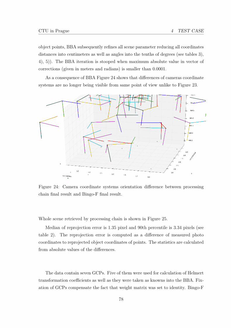
CTU in Prague 4 TEST CASE
object points, BBA subsequently refines all scene parameter reducing all coordinatesdistances into centimeters as well as angles into the tenths of degrees (see tables 3),4), 5)). The BBA iteration is stooped when maximum absolute value in vector ofcorrections (given in meters and radians) is smaller than 0.0001.
As a consequence of BBA Figure 24 shows that differences of cameras coordinatesystems are no longer being visible from same point of view unlike to Figure 23.
Figure 24: Camera coordinate systems orientation difference between processingchain final result and Bingo-F final result.
Whole scene retrieved by processing chain is shown in Figure 25.
Median of reprojection error is 1.35 pixel and 90th percentile is 3.34 pixels (seetable 2). The reprojection error is computed as a difference of measured photocoordinates to reprojected object coordinates of points. The statistics are calculatedfrom absolute values of the differences.
The data contain seven GCPs. Five of them were used for calculation of Helmerttransformation coefficients as well as they were taken as knowns into the BBA. Fix-ation of GCPs compensate the fact that weight matrix was set to identity. Bingo-F
78

CTU in Prague 4 TEST CASE
Figure 25: Final scene reconstruction by the developed processing chain.
uses probably some sophisticated algorithm how to set weights of the measurementsbecause clever setting of the weights can significantly improve accuracy obtainedfrom BBA.
Two randomly chosen GCPs were treated as tie points during whole processing.Resulting object coordinates were compared to the known coordinates of the twoGCPs. Also same comparison was done with the coordinates from Bingo-F results.The calculated coordinates are closer to the known values (see table 1). It can notbe said that the obtained results are more accurate than results of Bingo-F aftercomparison of just two points. On the other hand being closer to real values is notbad sign at all.
If the scene is adjusted as free network without GCPs being fixed and with weightmatrix given as identity, differences to Bingo-F results increase. Mostly it affectsexterior orientation. For instance, average difference in photo position increasesfrom 4.8 cm to 8.4 cm.
79
CTU in Prague 5 FUTURE DEVELOPMENT
5 Future development
Work done in this thesis can be considered as prove of a concept outlining path offuture evolution of the orthorectification workflow in GRASS. In the current state,the developed processing chain can not be considered as generally working solution.
It was just tested on one scene where it gives reasonable results. I am sure that itwould not work successfully in other, more complicated scenes because the solutionis not robust enough.
In order to improve robustness of the processing chain, following suggestionsshould be considered:
• Relative orientations – there is no check whether relative orientation is suc-cessful or not. Some mechanism should be implemented assessing quality ofrelative orientation (probably according to reprojection error of object pointsor epipolar distance). Also it should be examined work of the five point al-gorithm with RANSAC loop on scenes with higher number of tie points thanin the test case. It may increase outliers elimination effect of RANSAC loopthanks to bigger sample (number of points) for testing the outlier/inlier crite-rion.
• Merging of relative orientations – if there is one wrong relative orientationwith lot of depended relative orientations, the error propagates up duringtransformation of depended orientations to the common relative coordinatesystem. Effect of such an inaccurate pair could be reduced by performing freenetwork BBA during the transformation which can reduce the inaccuracies.Small errors can be serious issue likewise because they can sum up in longtransformation chains. Order of transformation of relative orientations shouldnot be chosen only by number of tie points but it should take into accountalso quality of relative orientation.
• Calculation of scale – it is computed as a median from individual scales (see1.6.6) without any assessment for outliers. The blunder detection can be imple-mented in same way as it is in Bingo-F taking into account object coordinatesdifferences of corresponding points used for calculation of individual scales.
80
CTU in Prague 5 FUTURE DEVELOPMENT
• During final BBA, setting of weights is ignored because weight matrix is setto identity matrix. Good choice of weights during every least squares iterationcould be big leap towards robustness of the BBA increasing also accuracy.Another way how to improve final accuracy of BBA is skipping photo pointswith higher standard deviation than some threshold. The standard deviationcriterion can be assessed after every iteration.
Another big room for improvement is computational speed of the processingchain. One least squares iteration of BBA takes approximately 5 seconds in thetest case, which can be considered as very small compared to commonly the solvedscenes with hundreds of photos and thousands of object points. Bingo-F managesto go through whole workflow containing 3 iteration of BBA in just 2 seconds.
The bottleneck of BBA iteration is computation of inverse/pseudo inverse of nor-mal matrix. The size of the matrix is directly connected to a number of measuredphoto points. The inversed matrix of BBA is sparse (most of elements are zeros). Itis possible to use many optimization methods exploiting this property e.g. matrixfactorizations. Additional speeding up of the code can be achieved by reimplemen-tation of some parts in C programming language instead of currently used Python.However, it should be done as the last step when the part to be reimplemented istested, optimized and works well. Otherwise, it would be waste of time and energyif the code would not be eventually used.
Another option to be considered is employing of some free software BBA librariese.g:
• sba3 library or
• Simple Sparse Bundle Adjustment 4.
Both libraries are highly optimized, based on Levenberg–Marquardt algorithm.On the other hand, it would require to add new dependency into GRASS. Addingnew dependencies should be avoided because GRASS already relies on many soft-ware libraries making its installation difficult, because of countless combinations oflibraries and its versions. Moreover, it makes fixing of bugs more complicated, since
3http://users.ics.forth.gr/~lourakis/sba/4http://www.inf.ethz.ch/personal/chzach/opensource.html
81
CTU in Prague 5 FUTURE DEVELOPMENT
some of them depend only on certain version of a library or on a combination oflibraries.
The thesis outlines just rough architecture of the final solution. At this earlystage of prototype, there is no point in dealing with the interface, which can changelot of time during further development.
Another area for improvement not covered by the thesis is error analysis of sceneparameters and their effect on final results. It should be studied another non-linearleast squares algorithms as e.g. Levenberg–Marquardt or Gauss–Newton.
It was set up as one of the main goals that the solution should be general in termsof photos orientation. The goal was not completely fulfilled because collinearityequations relies on parametrization of camera orientation by Euler angles. It maycause numerical instabilities in certain direction (1.5.2) thus it must be changed intosome other representation. Unit quaternions seem to be best choice since they donot suffer form gimbal lock problem [31].
82
CTU in Prague 6 CONCLUSION
6 Conclusion
The path leading to the final solution presented in the thesis has not been straight-forward. In the name of the thesis, there is stated that BBA would be used only forrefining of exterior orientation. In the beginning of this semester, when the nameof the thesis had to be chosen, I thought that it is not big deal. I supposed enoughGCPs will be always available for every photo as well as interior orientation will beknown together with initial values of exterior orientation. This case would requirejust performing of BBA.
As I dived more into the topic, it became clear that it would not be so easy if thesolution should met up current needs for processing of photos obtained by UAVs.Thus, new goal was set up to come up with a solution as much general as possibleallowing to retrieve structure from photos with nearly no other information exceptinterior orientation.
The work gave me a chance to get hands on photogrammetry and computervision. I have become enchanted by elegance of both fields consisting in a way ofdevelopment of incredibly powerful methods based on simple principles. Anothergreat thing about the topic is that the results can be assessed by everybody since itis easy to recognize whether a retrieved structure resembles captured scene or not.
The thesis analyzed the current state of orthorectification in GRASS and roughlyoutlined the way of its modification, in order to meet up current needs. The de-veloped solution was tested on data containing small set of photos. The data wasalso processed in state of the art Bingo-F software whose results were consideredas reference. After comparison of both results, it can be concluded that the devel-oped processing chain achieved similar accuracy as Bingo-F. However, it should beconsidered only as prove of concept. It is far away from being employed in practice.
83
CTU in Prague REFERENCES
References
[1] Alexandre Alahi, Raphael Ortiz, and Pierre Vandergheynst. Freak: Fast retinakeypoint. In Computer Vision and Pattern Recognition (CVPR), 2012 IEEEConference on, pages 510–517. IEEE, 2012.
[2] L Barazzetti, F Remondino, and M Scaioni. Extraction of accurate tie points forautomated pose estimation of close-range blocks. In ISPRS Technical Commis-sion III Symposium on Photogrammetric Computer Vision and Image Analysis,2010.
[3] M Bäumker and FJ Heimes. New calibration and computing method for directgeoreferencing of image and scanner data using the position and angular data ofan hybrid inertial navigation system. In OEEPE Workshop, Integrated SensorOrientation, 2001.
[4] Marcel Brückner, Ferid Bajramovic, and Joachim Denzler. Experimental eval-uation of relative pose estimation algorithms. In VISAPP (2), pages 431–438,2008.
[5] Wikimedia Commons. How a pinhole camera works. http://commons.
wikimedia.org/wiki/File:Pinhole-camera.png, 2005. [Online; accessed 16-December-2013].
[6] Rodney Deakin. Rank of a Matrix. Technical report, Royal Melbourne Instituteof Technology, 2006.
[7] Brown Duane. Decentering distortion of lenses. Photogrammetric Engineering,32(3):444–462, 1966.
[8] Prof. Federico. The Mathematical Derivation of Least Squares. http:
//isites.harvard.edu/fs/docs/icb.topic515975.files/OLSDerivation.
pdf. [Online; accessed 04-November-2013].
[9] Germany GIP mbH of Aalen. Bingo-f. http://www.gcs-abc.com/bingof.htm.[Online; accessed 01-December-2013].
[10] Armin Grünn. Precision and reliability aspects in close-range photogrammetry.XIVth Congress for Photogrammetry, 1980.
84
CTU in Prague REFERENCES
[11] R. I. Hartley and A. Zisserman. Multiple View Geometry in Computer Vision.Cambridge University Press, ISBN: 0521540518, second edition, 2004.
[12] Christian Heipke. Automation of interior, relative, and absolute orientation.ISPRS journal of photogrammetry and remote sensing, 52(1):1–19, 1997.
[13] Thomas Läbe and Wolfgang Förstner. Geometric stability of low-cost digi-tal consumer cameras. In Proceedings of the 20th ISPRS Congress, Istanbul,Turkey, pages 528–535, 2004.
[14] Thomas Läbe and Wolfgang Förstner. Automatic relative orientation of images.Proceedings of the 5th Turkish-German Joint Geodetic Days, 29:31, 2006.
[15] Stefan Leutenegger, Margarita Chli, and Roland Y Siegwart. Brisk: Binaryrobust invariant scalable keypoints. In Computer Vision (ICCV), 2011 IEEEInternational Conference on, pages 2548–2555. IEEE, 2011.
[16] Markus Metz, GRASS Development Team. v.rectify. http://grass.
osgeo.org/grass70/manuals/v.rectify.html, 2013. [Online; accessed 08-December-2013].
[17] Leoš Mervart and Zdeněk Lukeš. Adjustment Calculus. Nakladatelství ČVUT,2007.
[18] Mike Baba, GRASS Development Team. i.ortho.photo module. http://grass.
osgeo.org/grass64/manuals/i.ortho.photo.html, 2013. [Online; accessed03-December-2013].
[19] E.M. Mikhail and F.E. Ackermann. Observations and least squares. IEP seriesin civil engineering. IEP, 1976.
[20] Markus Neteler, M Hamish Bowman, Martin Landa, and Markus Metz. GRASSGIS: a multi-purpose Open Source GIS. Environmental Modelling & Software,31:124–130, 2012.
[21] Markus Neteler and Helena Mitasova. Open Source GIS: A GRASS GIS Ap-proach. Springer, New York, 2008.
85
CTU in Prague REFERENCES
[22] David Nistér. An efficient solution to the five-point relative pose problem.Pattern Analysis and Machine Intelligence, IEEE Transactions on, 26(6):756–770, 2004.
[23] OpenCV.org. Camera calibration and 3d reconstruction. OpenCV 3.0.0-devdocumentation. http://docs.opencv.org/master/modules/calib3d/doc/
camera_calibration_and_3d_reconstruction.html, 2013. [Online; accessed25-November-2013].
[24] OpenCV.org. Camera calibration with opencv. OpenCV 3.0.0-dev doc-umentation. http://docs.opencv.org/master/doc/tutorials/calib3d/
camera_calibration/camera_calibration.html, 2013. [Online; accessed 25-November-2013].
[25] Karel Pavelka. Fotogrammetrie 10. Nakladatelství ČVUT, 2003.
[26] Karel Pavelka. Fotogrammetrie 20. Nakladatelství ČVUT, 2003.
[27] John Hendrix Perry. A synthesized directly georeferenced remote sensing tech-nique for small unmanned aerial vehicles. Master’s thesis, University of Florida,2009.
[28] Tobias Pietzsch. Robot, position estimation of a mobile and camera, usinga single vehicle-mounted. Technical report, Dept. of Computer Science, TUDresden, Germany, 2002.
[29] Duccio Rocchini, Markus Metz, Alessandro Frigeri, Luca Delucchi, Matteo Mar-cantonio, and Markus Neteler. Robust rectification of aerial photographs in anopen source environment. Computers & geosciences, 39:145–151, 2012.
[30] Duccio Rocchini and Markus Neteler. Let the four freedoms paradigm apply toecology. Trends in ecology & evolution, 27(6):310–311, 2012.
[31] Jochen Schmidt and Heinrich Niemann. Using Quaternions for Parametrizing3-D Rotations in Unconstrained Nonlinear Optimization.
[32] LE Sjöberg. Closed-form and iterative weighted least squares solutions ofHelmert transformation parameters. Journal of Geodetic Science, 3(1):7–11,2013.
86
CTU in Prague REFERENCES
[33] Henrik Stewenius, Christopher Engels, and David Nistér. Recent developmentson direct relative orientation. ISPRS Journal of Photogrammetry and RemoteSensing, 60(4):284–294, 2006.
[34] Gilbert Strang and Kai Borre. Linear Algebra, Geodesy, and GPS. Wellesley-Cambridge Press, 1997.
[35] Wikimedia Commons. A selection of normal distribution probability den-sity functions (pdfs). http://commons.wikimedia.org/wiki/File:Normal_
Distribution_PDF.svg, 2008. [Online; accessed 10-December-2013].
[36] Wikimedia Commons. Bezmiechowa airfield 3d digital surface model obtainedafter 1 day of pre-flight testing, 1hr of flight and 1 day of processing, usingpteryx uav. http://commons.wikimedia.org/wiki/File:Bezmiechowa_DSM_
3D_2010-05-29_Pteryx_UAV.jpg, 2010. [Online; accessed 14-December-2013].
[37] Wikimedia Commons. Landtagsprojekt mecklenburg-vorpommern2013. http://commons.wikimedia.org/wiki/File:Landtagsprojekt_
Mecklenburg-Vorpommern_2013_by-RaBoe_010.jpg, 2013. [Online; accessed17-December-2013].
[38] Wikipedia. Eight-point algorithm. http://en.wikipedia.org/wiki/SURF,2013. [Online; accessed 25-November-2013].
[39] Wikipedia. Ransac. http://en.wikipedia.org/wiki/RANSAC, 2013. [Online;accessed 26-November-2013].
[40] Wikipedia. Scale-invariant feature transform — Wikipedia, the free en-cyclopedia. http://en.wikipedia.org/wiki/Scale-invariant_feature_
transform, 2013. [Online; accessed 25-November-2013].
[41] Wikipedia. Surf — Wikipedia, the free encyclopedia. http://en.wikipedia.
org/wiki/SURF, 2013. [Online; accessed 25-November-2013].
[42] Zhengyou Zhang. A flexible new technique for camera calibration. PatternAnalysis and Machine Intelligence, IEEE Transactions on, 22(11):1330–1334,2000.
87

CTU in Prague REFERENCES
[43] Zhang Zhengyou. Emerging Topics in Computer Vision, chapter 2, pages 4–43.Prentice Hall PTR Upper Saddle River, 2004.
[44] Václav Čada. Přednáškové texty z Geodézie, 7.5 Souřadnicové výpočty v rov-ině. http://gis.zcu.cz/studium/gen1/html/ch07s05.html. [Online; ac-cessed 01-November-2013].
88
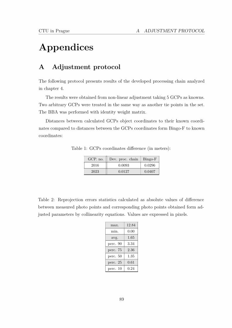
CTU in Prague A ADJUSTMENT PROTOCOL
Appendices
A Adjustment protocol
The following protocol presents results of the developed processing chain analyzedin chapter 4.
The results were obtained from non-linear adjustment taking 5 GCPs as knowns.Two arbitrary GCPs were treated in the same way as another tie points in the set.The BBA was performed with identity weight matrix.
Distances between calculated GCPs object coordinates to their known coordi-nates compared to distances between the GCPs coordinates form Bingo-F to knowncoordinates:
Table 1: GCPs coordinates difference (in meters):
GCP. no. Dev. proc. chain Bingo-F2016 0.0093 0.02962023 0.0127 0.0407
Table 2: Reprojection errors statistics calculated as absolute values of differencebetween measured photo points and corresponding photo points obtained form ad-justed parameters by collinearity equations. Values are expressed in pixels.
max. 12.84min. 0.00avg. 1.65
perc. 90 3.34perc. 75 2.36perc. 50 1.35perc. 25 0.61perc. 10 0.24
89
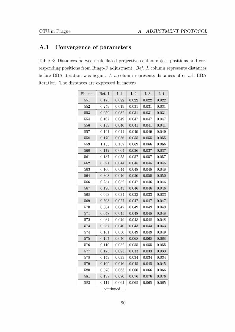
CTU in Prague A ADJUSTMENT PROTOCOL
A.1 Convergence of parameters
Table 3: Distances between calculated projective centers object positions and cor-responding positions from Bingo-F adjustment. Bef. I. column represents distancesbefore BBA iteration was begun. I. n column represents distances after nth BBAiteration. The distances are expressed in meters.
Ph. no. Bef. I. I. 1 I. 2 I. 3 I. 4551 0.173 0.022 0.022 0.022 0.022552 0.259 0.019 0.031 0.031 0.031553 0.059 0.032 0.031 0.031 0.031554 0.107 0.049 0.047 0.047 0.047556 0.139 0.040 0.041 0.041 0.041557 0.191 0.044 0.049 0.049 0.049558 0.170 0.056 0.055 0.055 0.055559 1.133 0.157 0.069 0.066 0.066560 0.172 0.064 0.036 0.037 0.037561 0.137 0.055 0.057 0.057 0.057562 0.021 0.044 0.045 0.045 0.045563 0.100 0.044 0.048 0.048 0.048564 0.303 0.046 0.050 0.050 0.050566 0.254 0.052 0.047 0.046 0.046567 0.190 0.043 0.046 0.046 0.046568 0.093 0.034 0.033 0.033 0.033569 0.508 0.027 0.047 0.047 0.047570 0.084 0.047 0.049 0.049 0.049571 0.048 0.045 0.048 0.048 0.048572 0.034 0.049 0.048 0.048 0.048573 0.057 0.040 0.043 0.043 0.043574 0.161 0.050 0.049 0.049 0.049575 0.197 0.070 0.068 0.068 0.068576 0.110 0.052 0.055 0.055 0.055577 0.175 0.023 0.033 0.033 0.033578 0.143 0.033 0.034 0.034 0.034579 0.109 0.046 0.045 0.045 0.045580 0.078 0.063 0.066 0.066 0.066581 0.197 0.070 0.076 0.076 0.076582 0.114 0.061 0.065 0.065 0.065
continued . . .
90
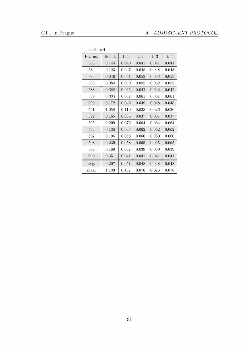
CTU in Prague A ADJUSTMENT PROTOCOL
. . . continuedPh. no. Bef. I. I. 1 I. 2 I. 3 I. 4583 0.144 0.040 0.041 0.041 0.041584 0.123 0.047 0.048 0.048 0.048585 0.046 0.051 0.053 0.053 0.053586 0.080 0.050 0.052 0.052 0.052588 0.388 0.035 0.042 0.042 0.042589 0.334 0.067 0.061 0.061 0.061590 0.172 0.042 0.049 0.048 0.048591 1.058 0.110 0.028 0.026 0.026592 0.165 0.035 0.037 0.037 0.037595 0.209 0.072 0.064 0.064 0.064596 0.138 0.063 0.062 0.062 0.062597 0.196 0.058 0.060 0.060 0.060598 0.239 0.058 0.065 0.065 0.065599 0.169 0.037 0.039 0.039 0.039600 0.351 0.041 0.041 0.041 0.041
avg. 0.207 0.051 0.048 0.048 0.048max. 1.133 0.157 0.076 0.076 0.076
91
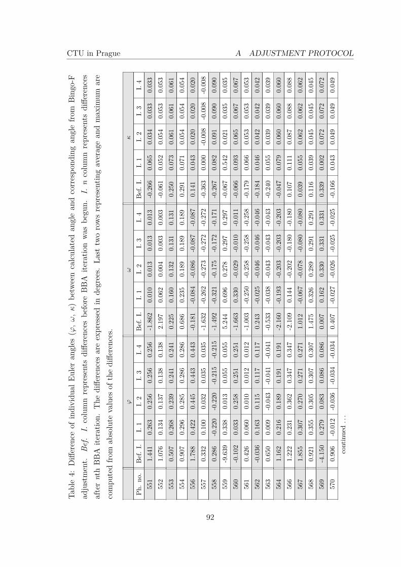
CTU in Prague A ADJUSTMENT PROTOCOL
Table4:
Difference
ofindividu
alEu
leran
gles
(ϕ,ω
,κ)be
tweencalculated
anglean
dcorrespo
ndingan
glefro
mBing
o-F
adjustment.
Bef.
I.columnrepresents
diffe
rences
before
BBA
iteratio
nwa
sbe
gun.
I.n
columnrepresents
diffe
rences
afternthBB
Aite
ratio
n.The
diffe
rences
areexpressedin
degrees.
Last
tworowsrepresentin
gaveragean
dmax
imum
are
compu
tedfro
mab
solute
values
ofthediffe
rences.
ϕω
κ
Ph.no
.Bef.I.
I.1
I.2
I.3
I.4
Bef.I.
I.1
I.2
I.3
I.4
Bef.I.
I.1
I.2
I.3
I.4
551
1.441
0.263
0.256
0.256
0.256
-1.862
0.010
0.013
0.013
0.013
-0.266
0.065
0.034
0.033
0.033
552
1.076
0.134
0.137
0.138
0.138
2.197
0.062
0.004
0.003
0.003
-0.061
0.052
0.054
0.053
0.053
553
0.507
0.268
0.239
0.241
0.241
0.225
0.160
0.132
0.131
0.131
0.250
0.073
0.061
0.061
0.061
554
0.907
0.296
0.285
0.286
0.286
0.686
0.235
0.189
0.189
0.189
0.291
0.071
0.054
0.054
0.054
556
1.788
0.422
0.445
0.443
0.443
-0.181
-0.084
-0.086
-0.087
-0.087
0.141
0.043
0.020
0.020
0.020
557
0.332
0.100
0.032
0.035
0.035
-1.632
-0.262
-0.273
-0.272
-0.272
-0.363
0.000
-0.008
-0.008
-0.008
558
0.286
-0.220
-0.220
-0.215
-0.215
-1.492
-0.321
-0.175
-0.172
-0.171
-0.267
0.082
0.091
0.090
0.090
559
-9.639
0.338
0.013
0.055
0.055
5.244
0.696
0.278
0.297
0.297
-0.067
0.542
0.021
0.035
0.035
560
-0.102
0.033
0.258
0.251
0.251
-1.663
0.330
-0.029
-0.010
-0.011
-0.066
0.093
0.065
0.067
0.067
561
0.426
0.060
0.010
0.012
0.012
-1.003
-0.250
-0.258
-0.258
-0.258
-0.179
0.066
0.053
0.053
0.053
562
-0.036
0.163
0.115
0.117
0.117
0.243
-0.025
-0.046
-0.046
-0.046
-0.184
0.046
0.042
0.042
0.042
563
0.650
0.009
-0.043
-0.041
-0.041
-0.533
-0.038
-0.043
-0.043
-0.043
-0.240
0.055
0.039
0.039
0.039
564
1.162
0.216
0.189
0.191
0.191
-2.160
-0.193
-0.203
-0.203
-0.203
-0.047
0.079
0.060
0.060
0.060
566
1.222
0.231
0.362
0.347
0.347
-2.109
0.144
-0.202
-0.180
-0.180
0.107
0.111
0.087
0.088
0.088
567
1.855
0.307
0.270
0.271
0.271
1.012
-0.067
-0.078
-0.080
-0.080
0.039
0.055
0.062
0.062
0.062
568
0.921
0.355
0.305
0.307
0.307
1.475
0.326
0.289
0.291
0.291
0.116
0.039
0.045
0.045
0.045
569
-4.150
0.279
0.083
0.086
0.086
0.007
0.162
0.330
0.331
0.331
0.339
0.002
0.072
0.072
0.072
570
0.906
-0.012
-0.036
-0.034
-0.034
0.407
-0.027
-0.026
-0.025
-0.025
-0.166
0.043
0.049
0.049
0.049
continued...
92
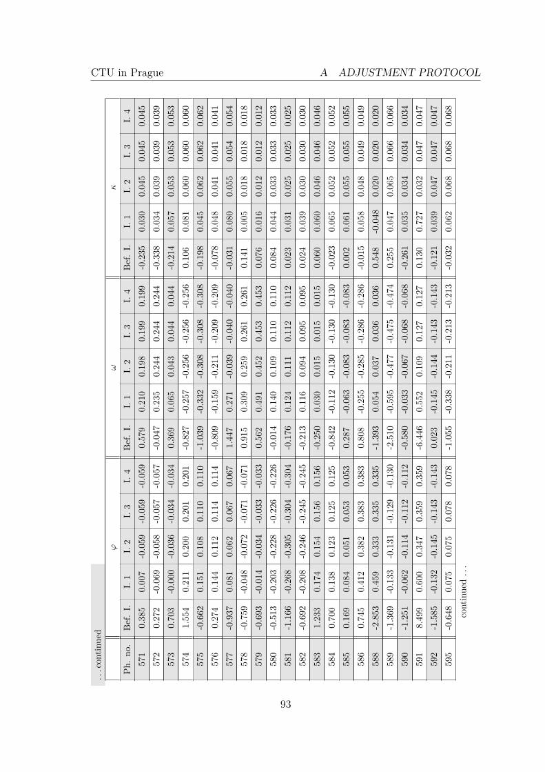
CTU in Prague A ADJUSTMENT PROTOCOL
...con
tinued
ϕω
κ
Ph.no
.Bef.I.
I.1
I.2
I.3
I.4
Bef.I.
I.1
I.2
I.3
I.4
Bef.I.
I.1
I.2
I.3
I.4
571
0.385
0.007
-0.059
-0.059
-0.059
0.579
0.210
0.198
0.199
0.199
-0.235
0.030
0.045
0.045
0.045
572
0.272
-0.069
-0.058
-0.057
-0.057
-0.047
0.235
0.244
0.244
0.244
-0.338
0.034
0.039
0.039
0.039
573
0.703
-0.000
-0.036
-0.034
-0.034
0.369
0.065
0.043
0.044
0.044
-0.214
0.057
0.053
0.053
0.053
574
1.554
0.211
0.200
0.201
0.201
-0.827
-0.257
-0.256
-0.256
-0.256
0.106
0.081
0.060
0.060
0.060
575
-0.662
0.151
0.108
0.110
0.110
-1.039
-0.332
-0.308
-0.308
-0.308
-0.198
0.045
0.062
0.062
0.062
576
0.274
0.144
0.112
0.114
0.114
-0.809
-0.159
-0.211
-0.209
-0.209
-0.078
0.048
0.041
0.041
0.041
577
-0.937
0.081
0.062
0.067
0.067
1.447
0.271
-0.039
-0.040
-0.040
-0.031
0.080
0.055
0.054
0.054
578
-0.759
-0.048
-0.072
-0.071
-0.071
0.915
0.309
0.259
0.261
0.261
0.141
0.005
0.018
0.018
0.018
579
-0.693
-0.014
-0.034
-0.033
-0.033
0.562
0.491
0.452
0.453
0.453
0.076
0.016
0.012
0.012
0.012
580
-0.513
-0.203
-0.228
-0.226
-0.226
-0.014
0.140
0.109
0.110
0.110
0.084
0.044
0.033
0.033
0.033
581
-1.166
-0.268
-0.305
-0.304
-0.304
-0.176
0.124
0.111
0.112
0.112
0.023
0.031
0.025
0.025
0.025
582
-0.692
-0.208
-0.246
-0.245
-0.245
-0.213
0.116
0.094
0.095
0.095
0.024
0.039
0.030
0.030
0.030
583
1.233
0.174
0.154
0.156
0.156
-0.250
0.030
0.015
0.015
0.015
0.060
0.060
0.046
0.046
0.046
584
0.700
0.138
0.123
0.125
0.125
-0.842
-0.112
-0.130
-0.130
-0.130
-0.023
0.065
0.052
0.052
0.052
585
0.169
0.084
0.051
0.053
0.053
0.287
-0.063
-0.083
-0.083
-0.083
0.002
0.061
0.055
0.055
0.055
586
0.745
0.412
0.382
0.383
0.383
0.808
-0.255
-0.285
-0.286
-0.286
-0.015
0.058
0.048
0.049
0.049
588
-2.853
0.459
0.333
0.335
0.335
-1.393
0.054
0.037
0.036
0.036
0.548
-0.048
0.020
0.020
0.020
589
-1.369
-0.133
-0.131
-0.129
-0.130
-2.510
-0.595
-0.477
-0.475
-0.474
0.255
0.047
0.065
0.066
0.066
590
-1.251
-0.062
-0.114
-0.112
-0.112
-0.580
-0.033
-0.067
-0.068
-0.068
-0.261
0.035
0.034
0.034
0.034
591
8.499
0.600
0.347
0.359
0.359
-6.446
0.552
0.109
0.127
0.127
0.130
0.727
0.032
0.047
0.047
592
-1.585
-0.132
-0.145
-0.143
-0.143
0.023
-0.145
-0.144
-0.143
-0.143
-0.121
0.039
0.047
0.047
0.047
595
-0.648
0.075
0.075
0.078
0.078
-1.055
-0.338
-0.211
-0.213
-0.213
-0.032
0.062
0.068
0.068
0.068
continued...
93
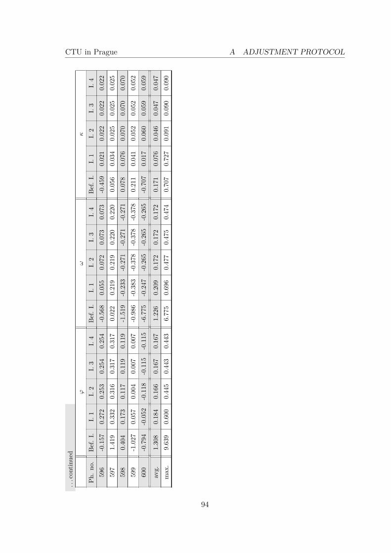
CTU in Prague A ADJUSTMENT PROTOCOL
...con
tinued
ϕω
κ
Ph.no
.Bef.I.
I.1
I.2
I.3
I.4
Bef.I.
I.1
I.2
I.3
I.4
Bef.I.
I.1
I.2
I.3
I.4
596
-0.157
0.272
0.253
0.254
0.254
-0.568
0.055
0.072
0.073
0.073
-0.459
0.021
0.022
0.022
0.022
597
1.419
0.332
0.316
0.317
0.317
0.022
0.219
0.219
0.220
0.220
0.056
0.034
0.025
0.025
0.025
598
0.404
0.173
0.117
0.119
0.119
-1.519
-0.233
-0.271
-0.271
-0.271
0.078
0.076
0.070
0.070
0.070
599
-1.027
0.057
0.004
0.007
0.007
-0.986
-0.383
-0.378
-0.378
-0.378
0.211
0.041
0.052
0.052
0.052
600
-0.794
-0.052
-0.118
-0.115
-0.115
-6.775
-0.247
-0.265
-0.265
-0.265
-0.707
0.017
0.060
0.059
0.059
avg.
1.308
0.184
0.166
0.167
0.167
1.226
0.209
0.172
0.172
0.172
0.171
0.076
0.046
0.047
0.047
max
.9.639
0.600
0.445
0.443
0.443
6.775
0.696
0.477
0.475
0.474
0.707
0.727
0.091
0.090
0.090
94
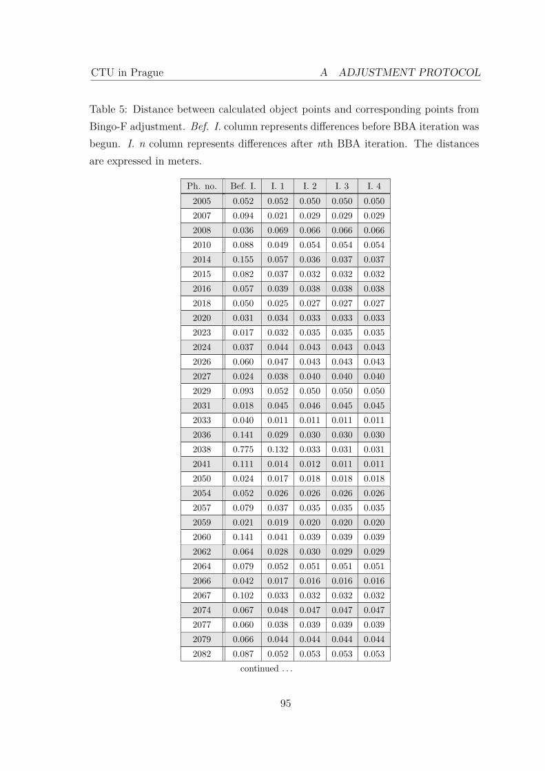
CTU in Prague A ADJUSTMENT PROTOCOL
Table 5: Distance between calculated object points and corresponding points fromBingo-F adjustment. Bef. I. column represents differences before BBA iteration wasbegun. I. n column represents differences after nth BBA iteration. The distancesare expressed in meters.
Ph. no. Bef. I. I. 1 I. 2 I. 3 I. 42005 0.052 0.052 0.050 0.050 0.0502007 0.094 0.021 0.029 0.029 0.0292008 0.036 0.069 0.066 0.066 0.0662010 0.088 0.049 0.054 0.054 0.0542014 0.155 0.057 0.036 0.037 0.0372015 0.082 0.037 0.032 0.032 0.0322016 0.057 0.039 0.038 0.038 0.0382018 0.050 0.025 0.027 0.027 0.0272020 0.031 0.034 0.033 0.033 0.0332023 0.017 0.032 0.035 0.035 0.0352024 0.037 0.044 0.043 0.043 0.0432026 0.060 0.047 0.043 0.043 0.0432027 0.024 0.038 0.040 0.040 0.0402029 0.093 0.052 0.050 0.050 0.0502031 0.018 0.045 0.046 0.045 0.0452033 0.040 0.011 0.011 0.011 0.0112036 0.141 0.029 0.030 0.030 0.0302038 0.775 0.132 0.033 0.031 0.0312041 0.111 0.014 0.012 0.011 0.0112050 0.024 0.017 0.018 0.018 0.0182054 0.052 0.026 0.026 0.026 0.0262057 0.079 0.037 0.035 0.035 0.0352059 0.021 0.019 0.020 0.020 0.0202060 0.141 0.041 0.039 0.039 0.0392062 0.064 0.028 0.030 0.029 0.0292064 0.079 0.052 0.051 0.051 0.0512066 0.042 0.017 0.016 0.016 0.0162067 0.102 0.033 0.032 0.032 0.0322074 0.067 0.048 0.047 0.047 0.0472077 0.060 0.038 0.039 0.039 0.0392079 0.066 0.044 0.044 0.044 0.0442082 0.087 0.052 0.053 0.053 0.053
continued . . .
95
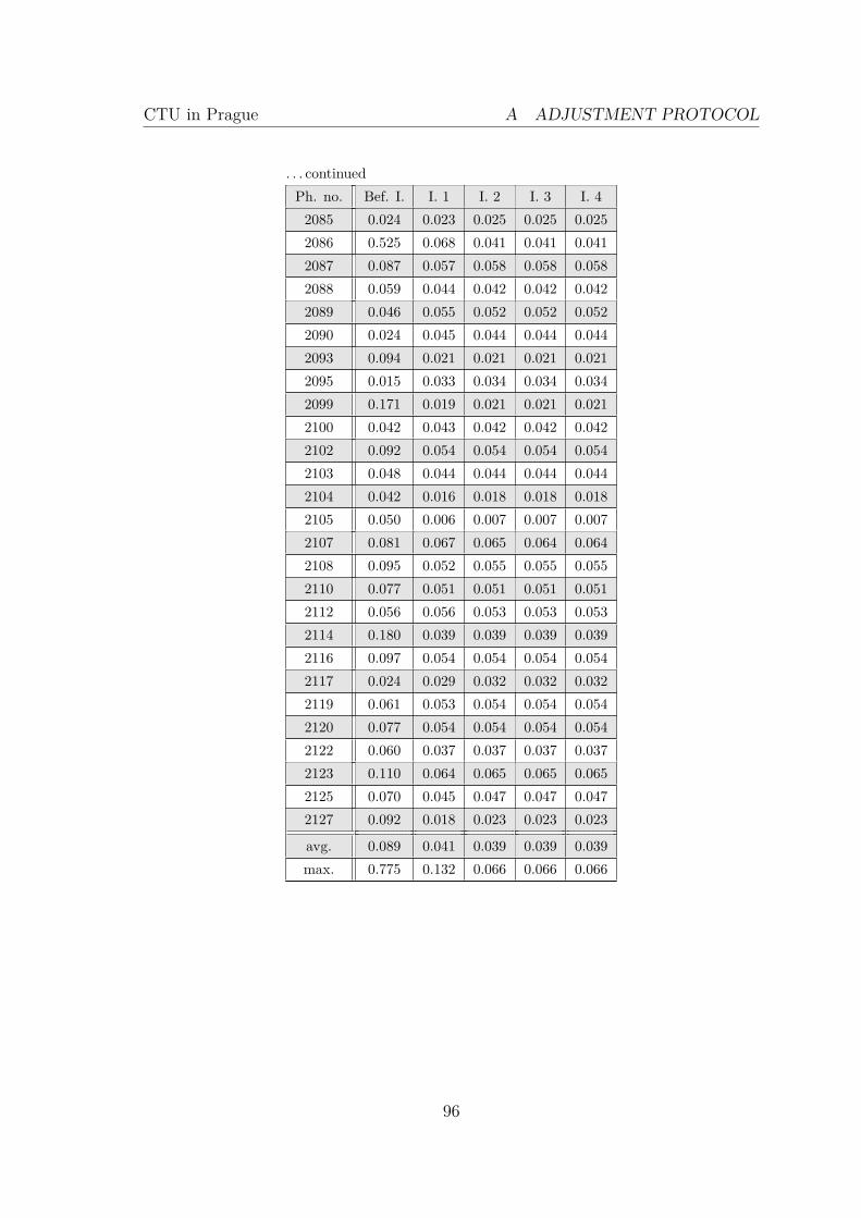
CTU in Prague A ADJUSTMENT PROTOCOL
. . . continuedPh. no. Bef. I. I. 1 I. 2 I. 3 I. 42085 0.024 0.023 0.025 0.025 0.0252086 0.525 0.068 0.041 0.041 0.0412087 0.087 0.057 0.058 0.058 0.0582088 0.059 0.044 0.042 0.042 0.0422089 0.046 0.055 0.052 0.052 0.0522090 0.024 0.045 0.044 0.044 0.0442093 0.094 0.021 0.021 0.021 0.0212095 0.015 0.033 0.034 0.034 0.0342099 0.171 0.019 0.021 0.021 0.0212100 0.042 0.043 0.042 0.042 0.0422102 0.092 0.054 0.054 0.054 0.0542103 0.048 0.044 0.044 0.044 0.0442104 0.042 0.016 0.018 0.018 0.0182105 0.050 0.006 0.007 0.007 0.0072107 0.081 0.067 0.065 0.064 0.0642108 0.095 0.052 0.055 0.055 0.0552110 0.077 0.051 0.051 0.051 0.0512112 0.056 0.056 0.053 0.053 0.0532114 0.180 0.039 0.039 0.039 0.0392116 0.097 0.054 0.054 0.054 0.0542117 0.024 0.029 0.032 0.032 0.0322119 0.061 0.053 0.054 0.054 0.0542120 0.077 0.054 0.054 0.054 0.0542122 0.060 0.037 0.037 0.037 0.0372123 0.110 0.064 0.065 0.065 0.0652125 0.070 0.045 0.047 0.047 0.0472127 0.092 0.018 0.023 0.023 0.023
avg. 0.089 0.041 0.039 0.039 0.039max. 0.775 0.132 0.066 0.066 0.066
96
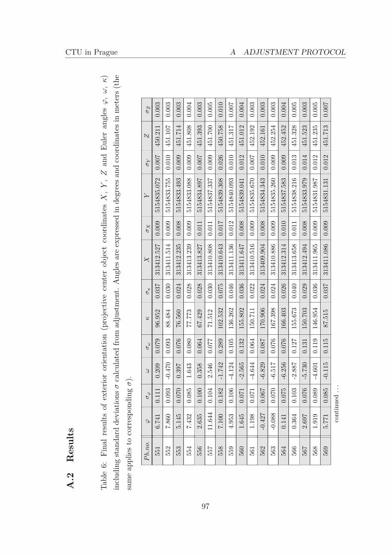
CTU in Prague A ADJUSTMENT PROTOCOL
A.2
Results
Table6:
Fina
lresults
ofexterio
rorientation
(projectivecenter
object
coordina
tesX,Y,Z
and
Euleran
glesϕ,ω,κ)
includ
ingstan
dard
deviationsσcalculated
from
adjustment.
Ang
lesa
reexpressedin
degreesa
ndcoordina
tesinmeters(
the
sameap
pliesto
correspo
ndingσ).
Ph.no.
ϕσϕ
ωσω
κσκ
XσX
YσY
ZσZ
551
6.741
0.111
0.209
0.079
96.952
0.037
313412.527
0.009
5154835.072
0.007
450.211
0.003
552
7.860
0.093
-0.470
0.093
88.484
0.030
313411.514
0.009
5154833.755
0.010
451.107
0.003
553
5.145
0.070
0.397
0.076
76.560
0.024
313412.235
0.008
5154833.493
0.009
451.714
0.003
554
7.432
0.085
1.643
0.080
77.773
0.028
313413.239
0.009
5154833.088
0.009
451.808
0.004
556
2.635
0.100
0.358
0.064
67.429
0.028
313413.827
0.011
5154834.897
0.007
451.393
0.003
557
11.644
0.104
2.546
0.077
71.512
0.030
313410.808
0.011
5154837.337
0.009
451.700
0.005
558
7.100
0.182
-1.742
0.289
102.532
0.075
313410.643
0.017
5154839.308
0.026
450.758
0.010
559
4.953
0.106
-4.124
0.105
136.262
0.046
313411.136
0.012
5154840.093
0.010
451.317
0.007
560
1.645
0.071
-2.565
0.132
155.802
0.036
313411.647
0.008
5154839.041
0.012
451.012
0.004
561
1.198
0.071
-4.644
0.064
150.711
0.022
313410.516
0.009
5154835.670
0.007
452.192
0.003
562
-0.427
0.067
-6.829
0.087
170.906
0.024
313409.904
0.008
5154834.343
0.010
452.161
0.003
563
-0.088
0.070
-6.517
0.076
167.398
0.024
313410.886
0.009
5154835.260
0.009
452.254
0.003
564
0.141
0.075
-6.256
0.076
166.403
0.026
313412.314
0.010
5154837.583
0.009
452.452
0.004
566
0.364
0.103
-2.887
0.127
155.673
0.040
313413.658
0.011
5154838.216
0.013
451.328
0.005
567
2.697
0.076
-5.730
0.131
150.703
0.029
313412.494
0.008
5154833.979
0.014
451.523
0.003
568
1.919
0.089
-4.601
0.119
146.954
0.036
313411.965
0.009
5154831.987
0.012
451.235
0.005
569
5.771
0.085
-0.115
0.115
87.515
0.037
313411.086
0.009
5154831.131
0.012
451.713
0.007
continued...
97
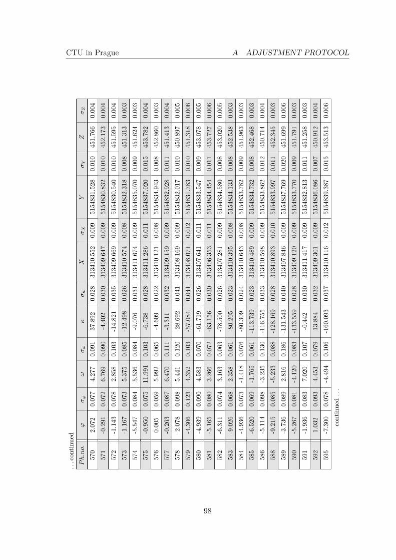
CTU in Prague A ADJUSTMENT PROTOCOL
...con
tinued
Ph.no.
ϕσϕ
ωσω
κσκ
XσX
YσY
ZσZ
570
2.072
0.077
4.277
0.091
37.892
0.028
313410.552
0.009
5154831.528
0.010
451.766
0.004
571
-0.291
0.072
6.769
0.090
-4.402
0.030
313409.647
0.009
5154830.832
0.010
452.173
0.004
572
-1.143
0.078
2.858
0.103
-14.821
0.035
313409.669
0.009
5154830.540
0.010
451.595
0.004
573
-1.167
0.073
5.375
0.085
-12.498
0.026
313410.574
0.008
5154832.318
0.008
451.313
0.003
574
-5.547
0.084
5.536
0.084
-9.076
0.031
313411.674
0.009
5154835.070
0.009
451.624
0.003
575
-0.950
0.075
11.991
0.103
-6.738
0.028
313411.286
0.011
5154837.020
0.015
453.782
0.004
576
0.005
0.059
5.992
0.065
-4.609
0.022
313410.121
0.008
5154834.943
0.008
452.860
0.003
577
-0.263
0.087
6.470
0.111
-3.311
0.032
313409.159
0.009
5154832.928
0.011
451.413
0.004
578
-2.078
0.098
5.441
0.120
-28.692
0.041
313408.169
0.009
5154832.017
0.010
450.897
0.005
579
-4.306
0.123
4.352
0.103
-57.084
0.041
313408.071
0.012
5154831.783
0.010
451.318
0.006
580
-4.939
0.090
4.583
0.070
-61.719
0.026
313407.641
0.011
5154833.547
0.009
453.078
0.005
581
-5.165
0.080
3.266
0.072
-63.156
0.030
313406.353
0.011
5154834.454
0.011
453.727
0.006
582
-6.311
0.074
3.163
0.063
-78.500
0.026
313407.281
0.009
5154834.580
0.008
453.020
0.005
583
-9.026
0.068
2.358
0.061
-80.205
0.023
313410.395
0.008
5154834.133
0.008
452.538
0.003
584
-4.936
0.073
-1.418
0.076
-80.309
0.024
313410.643
0.008
5154833.782
0.009
451.963
0.003
585
-6.520
0.069
-1.765
0.061
-113.739
0.023
313410.489
0.009
5154834.732
0.008
452.468
0.003
586
-5.114
0.098
-3.235
0.130
-116.755
0.033
313410.598
0.009
5154833.862
0.012
450.714
0.004
588
-9.215
0.085
-5.233
0.088
-128.169
0.028
313410.893
0.010
5154833.997
0.011
452.345
0.003
589
-3.736
0.089
2.816
0.186
-131.543
0.040
313407.846
0.009
5154837.769
0.020
451.699
0.006
590
-5.267
0.081
-4.120
0.083
-133.559
0.028
313409.120
0.009
5154833.770
0.009
451.791
0.003
591
-1.936
0.083
7.020
0.107
-0.442
0.030
313411.417
0.009
5154832.813
0.011
451.258
0.003
592
1.032
0.093
4.453
0.079
13.884
0.032
313409.301
0.009
5154836.086
0.007
450.912
0.004
595
-7.300
0.078
-4.494
0.106
-160.093
0.037
313410.116
0.012
5154839.387
0.015
453.513
0.006
continued...
98
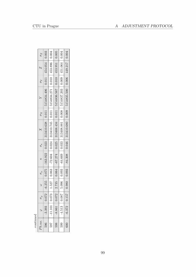
CTU in Prague A ADJUSTMENT PROTOCOL
...con
tinued
Ph.no.
ϕσϕ
ωσω
κσκ
XσX
YσY
ZσZ
596
-3.393
0.072
-6.255
0.075
-163.922
0.023
313410.638
0.011
5154834.406
0.011
454.054
0.003
597
-11.101
0.073
1.527
0.063
-72.604
0.024
313410.745
0.011
5154834.271
0.010
453.896
0.004
598
-8.861
0.072
2.735
0.064
-67.274
0.025
313408.434
0.011
5154836.567
0.010
453.951
0.005
599
-4.513
0.087
5.096
0.093
-64.669
0.033
313408.881
0.008
5154837.203
0.009
451.064
0.004
600
-6.372
0.157
0.980
0.093
-84.308
0.046
313410.680
0.009
5154835.500
0.006
449.217
0.004
99
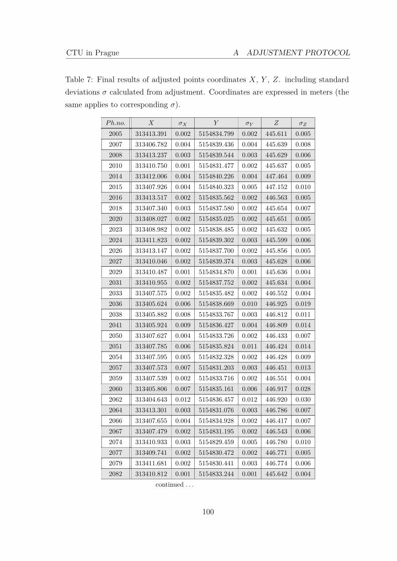
CTU in Prague A ADJUSTMENT PROTOCOL
Table 7: Final results of adjusted points coordinates X, Y , Z. including standarddeviations σ calculated from adjustment. Coordinates are expressed in meters (thesame applies to corresponding σ).
Ph.no. X σX Y σY Z σZ
2005 313413.391 0.002 5154834.799 0.002 445.611 0.0052007 313406.782 0.004 5154839.436 0.004 445.639 0.0082008 313413.237 0.003 5154839.544 0.003 445.629 0.0062010 313410.750 0.001 5154831.477 0.002 445.637 0.0052014 313412.006 0.004 5154840.226 0.004 447.464 0.0092015 313407.926 0.004 5154840.323 0.005 447.152 0.0102016 313413.517 0.002 5154835.562 0.002 446.563 0.0052018 313407.340 0.003 5154837.580 0.002 445.654 0.0072020 313408.027 0.002 5154835.025 0.002 445.651 0.0052023 313408.982 0.002 5154838.485 0.002 445.632 0.0052024 313411.823 0.002 5154839.302 0.003 445.599 0.0062026 313413.147 0.002 5154837.700 0.002 445.856 0.0052027 313410.046 0.002 5154839.374 0.003 445.628 0.0062029 313410.487 0.001 5154834.870 0.001 445.636 0.0042031 313410.955 0.002 5154837.752 0.002 445.634 0.0042033 313407.575 0.002 5154835.482 0.002 446.552 0.0042036 313405.624 0.006 5154838.669 0.010 446.925 0.0192038 313405.882 0.008 5154833.767 0.003 446.812 0.0112041 313405.924 0.009 5154836.427 0.004 446.809 0.0142050 313407.627 0.004 5154833.726 0.002 446.433 0.0072051 313407.785 0.006 5154835.824 0.011 446.424 0.0142054 313407.595 0.005 5154832.328 0.002 446.428 0.0092057 313407.573 0.007 5154831.203 0.003 446.451 0.0132059 313407.539 0.002 5154833.716 0.002 446.551 0.0042060 313405.806 0.007 5154835.161 0.006 446.917 0.0282062 313404.643 0.012 5154836.457 0.012 446.920 0.0302064 313413.301 0.003 5154831.076 0.003 446.786 0.0072066 313407.655 0.004 5154834.928 0.002 446.417 0.0072067 313407.479 0.002 5154831.195 0.002 446.543 0.0062074 313410.933 0.003 5154829.459 0.005 446.780 0.0102077 313409.741 0.002 5154830.472 0.002 446.771 0.0052079 313411.681 0.002 5154830.441 0.003 446.774 0.0062082 313410.812 0.001 5154833.244 0.001 445.642 0.004
continued . . .
100
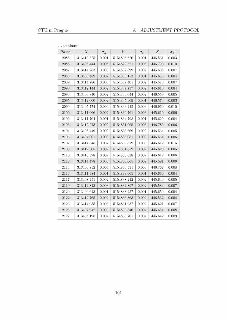
CTU in Prague A ADJUSTMENT PROTOCOL
. . . continuedPh.no. X σX Y σY Z σZ
2085 313410.325 0.001 5154836.620 0.001 446.561 0.0032086 313406.444 0.006 5154829.521 0.005 446.790 0.0102087 313414.283 0.003 5154832.899 0.002 445.608 0.0072088 313408.489 0.002 5154833.153 0.001 445.655 0.0042089 313414.786 0.003 5154837.401 0.002 445.578 0.0072090 313412.144 0.002 5154837.737 0.002 445.610 0.0042093 313406.840 0.002 5154833.044 0.002 446.559 0.0052095 313412.000 0.002 5154835.909 0.001 446.573 0.0032099 313405.774 0.004 5154833.215 0.003 446.960 0.0102100 313411.066 0.002 5154839.761 0.003 445.610 0.0062102 313411.704 0.001 5154834.798 0.001 445.629 0.0042103 313412.273 0.002 5154831.065 0.003 446.786 0.0062104 313408.449 0.002 5154836.669 0.002 446.564 0.0052105 313407.001 0.003 5154836.081 0.002 446.554 0.0062107 313414.845 0.007 5154839.879 0.006 445.612 0.0152108 313412.505 0.002 5154831.859 0.002 445.628 0.0052110 313413.378 0.002 5154833.038 0.002 445.612 0.0062112 313414.478 0.003 5154836.065 0.002 445.591 0.0062114 313406.752 0.004 5154830.531 0.003 446.767 0.0082116 313411.984 0.001 5154833.605 0.001 445.630 0.0042117 313408.451 0.002 5154838.212 0.002 445.649 0.0052119 313414.843 0.003 5154834.897 0.002 445.584 0.0072120 313409.643 0.001 5154833.257 0.001 445.650 0.0042122 313412.765 0.002 5154836.863 0.002 446.562 0.0042123 313414.055 0.003 5154831.937 0.002 445.621 0.0072125 313407.942 0.003 5154839.846 0.004 445.654 0.0082127 313406.198 0.004 5154838.701 0.004 445.642 0.009
101