cydar user guide - cydarex | core and cuttings analysis ... · cydarex cydar user manual 21...
TRANSCRIPT

CYDAR
USER MANUAL
CYDAR
USER MANUAL

CYDAREX CYDAR User Manual 21 September 2016
2

CYDAREX CYDAR User Manual 21 September 2016
3
CYDAR USER MANUAL
CYDAR – USER MANUAL ................................................................................................................................ 3
INSTALLATION OF CYDAR ............................................................................................................................ 7
SYSTEM REQUIREMENTS ..................................................................................................................................... 7 INSTALLATION OF CYDAR ................................................................................................................................ 7 PROBLEMS WITH THE INSTALLATION .................................................................................................................. 7 UPDATING CYDAR ............................................................................................................................................ 8 UNINSTALLING CYDAR .................................................................................................................................... 8 SILENT INSTALL AND UNINSTALL OF CYDAR ................................................................................................... 8
CYDAR OVERVIEW .......................................................................................................................................... 9
MERCURY INJECTION (MICP) ............................................................................................................................ 9 ABSOLUTE PERMEABILITY................................................................................................................................ 10 TWO-PHASE FLOW EXPERIMENT ...................................................................................................................... 10 RELATIVE PERMEABILITY ................................................................................................................................. 11 CENTRIFUGE CAPILLARY PRESSURE .................................................................................................................. 11 CYDAR MAIN FEATURES ................................................................................................................................. 12
Windows environment ................................................................................................................................. 12 Data input ................................................................................................................................................... 12 Numerical calculation ................................................................................................................................. 12 Exporting results ......................................................................................................................................... 12 Data smoothing ........................................................................................................................................... 12 Graphical display ........................................................................................................................................ 13 Reporting ..................................................................................................................................................... 13
CYDAR FUNCTIONALITIES ......................................................................................................................... 14
OPENING AND SAVING PROJECTS ...................................................................................................................... 14 AUTOSAVE SETTINGS ....................................................................................................................................... 14 IMPORTING DATA ............................................................................................................................................. 14 READING ASCII FILES ...................................................................................................................................... 15 LOADING DATA IN CYDAR .............................................................................................................................. 15 UNITS ............................................................................................................................................................... 15 NUMBER FORMAT ............................................................................................................................................. 16 DATA EDITING .................................................................................................................................................. 16 DATA SMOOTHING ............................................................................................................................................ 17
Principle of data smoothing ........................................................................................................................ 17 Curve fitting ................................................................................................................................................ 17
Interpolations (curve passes by all data points) ........................................................................................................ 17 Spline Fits (curve does not pass by all data points) .................................................................................................. 18 Fit functions ............................................................................................................................................................. 18 Multi-step fits ........................................................................................................................................................... 20
GRAPHS ............................................................................................................................................................ 21 Edit Points graph ........................................................................................................................................ 21 XY Graph .................................................................................................................................................... 21 Scaling up and scaling down a graph selection .......................................................................................... 22 Moving the display zone .............................................................................................................................. 22 Editing a graph ........................................................................................................................................... 22 Reticles ........................................................................................................................................................ 22
EXPORTING RESULTS ........................................................................................................................................ 23
CYDAREX CYDAR User Manual 21 September 2016
4
Graph .......................................................................................................................................................... 23 Simulation and analytical data ................................................................................................................... 23 Reporting ..................................................................................................................................................... 23 Copying a graph or a frame ........................................................................................................................ 25
NEW PROJECT WINDOW .............................................................................................................................. 26
MERCURY INJECTION MODULE ............................................................................................................... 27
MERCURY MAIN WINDOW ................................................................................................................................. 27 MERCURY TYPES OF CURVES ............................................................................................................................ 28 PORE SIZE DISTRIBUTION .................................................................................................................................. 28 PERMEABILITY CALCULATION .......................................................................................................................... 29 CAPILLARY PRESSURE FROM MERCURY ............................................................................................................ 30
J Leverett Function ..................................................................................................................................... 30 Transition zones .......................................................................................................................................... 31 Water cut ..................................................................................................................................................... 31
TUTORIAL FILES ................................................................................................................................................ 31 Tutorial_Hg_SampleA ................................................................................................................................ 31 Tutorial_Hg_Brauvillier ............................................................................................................................. 31
PERMEABILITY MODULE ............................................................................................................................ 32
PERMEABILITY MAIN WINDOW ......................................................................................................................... 32 SAMPLE AND FLUID PROPERTIES ....................................................................................................................... 32 KLINKENBERG CORRELATIONS ......................................................................................................................... 33 STEADY-STATE EXPERIMENT ............................................................................................................................ 33
Data points steady-state .............................................................................................................................. 33 Calculate permeability: steady-state ........................................................................................................... 34 Inertial correction ....................................................................................................................................... 35 Klinkenberg correction ............................................................................................................................... 36 Tubing correction ........................................................................................................................................ 36
TRANSIENT EXPERIMENT .................................................................................................................................. 36 Data points transient / unsteady state ......................................................................................................... 36 Permeability pulse decay ............................................................................................................................ 37 Parameter menu transient: ......................................................................................................................... 38
TUTORIAL FILES ................................................................................................................................................ 38 Tutorial_Perm_Klinkenberg ....................................................................................................................... 38 Tutorial_Perm_Inertial ............................................................................................................................... 38 Tutorial_PERM_Pulse_decay_Analytical................................................................................................... 39
TWO-PHASE FLOW MODULE ...................................................................................................................... 40
Two-phase flow: direct simulations ............................................................................................................ 41 Fluids and sample properties ...................................................................................................................... 41 Capillary pressure: Pc ................................................................................................................................ 42
Pc type ..................................................................................................................................................................... 42 “Data points” frame ................................................................................................................................................. 42 Analytical function ................................................................................................................................................... 42 Amott Index ............................................................................................................................................................. 43
Relative permeabilities: Kr ......................................................................................................................... 43 End Points ................................................................................................................................................................ 43 Corey model ............................................................................................................................................................. 44 Modified Corey ........................................................................................................................................................ 44 LET Function ........................................................................................................................................................... 44
Load/fit data Window .................................................................................................................................. 45 Raw data .................................................................................................................................................................. 45 Data depending on Saturation .................................................................................................................................. 47 Data corrections ....................................................................................................................................................... 47 Correction volumes and flow rates ........................................................................................................................... 47
Type of experiment ...................................................................................................................................... 48 Block times .................................................................................................................................................. 49 Bond, Capillary, and Rapoport Numbers .................................................................................................... 49

CYDAREX CYDAR User Manual 21 September 2016
5
Inlet Face Capillary Pressure, PC ............................................................................................................... 50 View (curve display) .................................................................................................................................... 50 Local Pressures (version 2014) .................................................................................................................. 50
Loading the abscissas ............................................................................................................................................... 50 Graphs ...................................................................................................................................................................... 51
Interfacial tension and viscosities values per block time (version 2016) .................................................... 52 Values ...................................................................................................................................................................... 52 Enabling the IFT and viscosities change between block times in simulation ........................................................... 52 IFT change implementation ..................................................................................................................................... 53 Viscosity change implementation ............................................................................................................................ 53
NUMERICAL SIMULATION ................................................................................................................................. 54 OPTIMIZATION .................................................................................................................................................. 55
Objective function ....................................................................................................................................... 55 Optimization per points ............................................................................................................................... 56
Moving points .......................................................................................................................................................... 56 Optimization ............................................................................................................................................................ 57
UNSTEADY STATE ............................................................................................................................................. 58 Analytical methods (JBN) ........................................................................................................................... 58
Window JBN-Jones and Roszelle ............................................................................................................................ 58 Tutorial Kr_USS_MW ................................................................................................................................. 59
Starting a project ...................................................................................................................................................... 59 Kr calculation ........................................................................................................................................................... 60 Simulation with initial guess .................................................................................................................................... 61 Kr optimization ........................................................................................................................................................ 61
STEADY-STATE ................................................................................................................................................. 62 Analytical .................................................................................................................................................... 62 Tutorial ....................................................................................................................................................... 63
Starting a project ...................................................................................................................................................... 63 Simulation with first guess ....................................................................................................................................... 64 Kr optimization ........................................................................................................................................................ 64
CENTRIFUGE ..................................................................................................................................................... 65 Local Pc from average ................................................................................................................................ 65
Optimization tool ..................................................................................................................................................... 65 Tutorial Pc calculation: Comparison CYDAR – Forbes SCA ..................................................................... 66 Relative Permeability – Hagoort................................................................................................................. 71
The “centri Kr” window, Hagoort part ..................................................................................................................... 71 Corey fit ................................................................................................................................................................... 71 Tutorial Hagoort....................................................................................................................................................... 72
Multistep Kr ................................................................................................................................................ 73 Speed correction....................................................................................................................................................... 73
POROUS PLATE ................................................................................................................................................. 75 HETEROGENEITIES ............................................................................................................................................ 76
Heterogeneity data type .............................................................................................................................. 76 Homogeneous .......................................................................................................................................................... 76 Composite ................................................................................................................................................................ 76 Profiles ..................................................................................................................................................................... 77
Capillary pressure ....................................................................................................................................... 77 Simulation ................................................................................................................................................... 78
Composite ................................................................................................................................................................ 78 Profiles ..................................................................................................................................................................... 78
HYSTERESIS ...................................................................................................................................................... 79 Nomenclature and definitions used .......................................................................................................................... 79
Pc scanning imbibition curve ...................................................................................................................... 80 Pc scanning drainage curve ........................................................................................................................ 80 Loop ............................................................................................................................................................ 81 Relative permeabilities ................................................................................................................................ 81 Non-uniform initial saturation profile ......................................................................................................... 81
INERTIAL CORRECTION (VERSION 2014) ........................................................................................................... 81 ELECTRICAL (VERSION 2016) ........................................................................................................................... 82
Purpose ....................................................................................................................................................... 82 Principles .................................................................................................................................................... 82 Experimental setup possibilities .................................................................................................................. 82

CYDAREX CYDAR User Manual 21 September 2016
6
Rload at the inlet ...................................................................................................................................................... 83 Rload at the outlet .................................................................................................................................................... 83 Resistances calculation ............................................................................................................................................ 83 Contact resistances ................................................................................................................................................... 83 Saturation calculation ............................................................................................................................................... 84
CYDAR module ........................................................................................................................................... 84 Electrical method: setup window ............................................................................................................................. 84
The experimental data are resistances ................................................................................................................. 84 The experimental data are voltages ..................................................................................................................... 85
The current is directly entered ....................................................................................................................... 85 The current is calculated from other data ...................................................................................................... 85
Saturation calculation ......................................................................................................................................... 85 Input data ................................................................................................................................................................. 85 Output data ............................................................................................................................................................... 86
TPF REPORTING ............................................................................................................................................... 86 Principle of ASCII file ................................................................................................................................. 86 Using template: ........................................................................................................................................... 87
CURVE FITTING TOOL .................................................................................................................................. 89
APPENDICES ..................................................................................................................................................... 90
NUMERICAL METHODS ...................................................................................................................................... 90 Newton-Raphson method: ........................................................................................................................... 90 Euler implicit: ............................................................................................................................................. 90 Transient permeability module: .................................................................................................................. 91 Two-phase flow module: ............................................................................................................................. 91
RIGHT CLICK MENUS ......................................................................................................................................... 92 SHORTCUTS ...................................................................................................................................................... 93 TROUBLESHOOTING .......................................................................................................................................... 94
Error message during installation .............................................................................................................. 94 The installation software cannot be launch ................................................................................................ 94 Installation software gets stuck ................................................................................................................... 94 Text on CYDAR™ windows is impossible to read ...................................................................................... 94 Issues when copy-pasting with Excel .......................................................................................................... 95
REFERENCES ..................................................................................................................................................... 96

CYDAREX CYDAR User Manual 21 September 2016
7
This notice describes the functionalities of CYDAR. The first part details the installation procedure, gives an overview of CYDAR, and presents the main functionalities such as importing and exporting data, smoothing curves, displaying graphs. Each module is then presented. The relative permeability and centrifuge capillary pressure are part of the Two-Phase Flow module.
Other modules related to laboratory equipment with data acquisition boards (Darcylog, Darcypress, Centri) are described in separate manuals.
Installation of CYDAR
System requirements CYDAR is developed in Visual Basic, an object oriented language that takes advantage of the Windows graphic environment. CYDAR runs on a Microsoft Windows operating system, and has been fully tested on Windows XP, Windows Vista, Windows 7, 8, and 10. CYDAR does not require a powerful computer, and can be installed on a laptop or an older computer. CYDAR does not require access to the Internet.
Numerical calculations such as the optimization loops are developed in FORTRAN using the powerful IMSL library. However, there is only one program to install, and the user has no direct contact with the various
by CYDAR.
The use of data acquisition boards requires installation of the corresponding software. This operation is described in separate manual.
Installation of CYDAR Before installation, it is recommended to close all running applications.
Insert the installation software CD in your CD-Rom drive. The CD contains other folders (tutorials, User Manuals, etc.). If the installation CD does not start automatically, open your CD-Rom drive and double-click on setup.exe. For Windows Vista, Windows 7, 8, and 10,
mouse right click (even if you use an administrator account). If CYDAR was downloaded from the Internet, just double-click on the Install file.
On Windows 8 or Windows 10, your computer might require an Internet connection to finish the installation. Also, if the installation Microsoft data access components 2.0 (not
fine.
The installer will start. Click the "install" button and follow on-screen instructions.
Depending on the operating system, some messages might occur during installation. Choose the option ,
the existing file as recommended.
After the installation is completed, click "finish".
During the first utilization, a login and password will be required; contact CYDAREX if you do not have one.
project.
Problems with the Installation For problems with the installation of CYDAR, see the Troubleshooting section at the end of this manual.

CYDAREX CYDAR User Manual 21 September 2016
8
Updating CYDAR wnloaded from
CYDAREX website. The file to replace is usually located in C:\Program Files\CYDAR. Occasionally, a complete reinstallation of CYDAR might be required. In that case, it is recommended to first uninstall the software, and then perform a complete installation with the files downloaded from CYDAREX website.
Uninstalling CYDAR Windows control panel. Then select CYDAR and
Silent Install and Uninstall of CYDAR To install CYDAR in silent mode, type the following command line:
c:\CYDAR_Install_Folder_Path\setup.exe s c:\ CYDAR_Install_Folder_Path\CYDAR_Install.log
To uninstall CYDAR in silent mode, type:
St6unst -n "C:\Program Files\CYDAR\St6unst.log" -f -q
CYDAREX CYDAR User Manual 21 September 2016
9
CYDAR Overview
CYDAR has been developed in collaboration with core analysis specialists, with two main objectives:
To be user-friendly: This is achieved by using Windows environment with an intuitive graphic user interface, like any Microsoft software. CYDAR can be used with no specific knowledge in numerical simulation or reservoir engineering.
To be accurate and powerful: CYDAR uses the most recent methods developed and tested in research laboratories, and published in the proceedings of the Society of Core Analysis.
CYDAR contains the following modules for routine and special core analyses:
mercury injection and withdrawal (MICP),
absolute permeability,
two-phase flow experiments,
steady-state and unsteady-state relative permeability,
centrifuge capillary pressure and relative permeability.
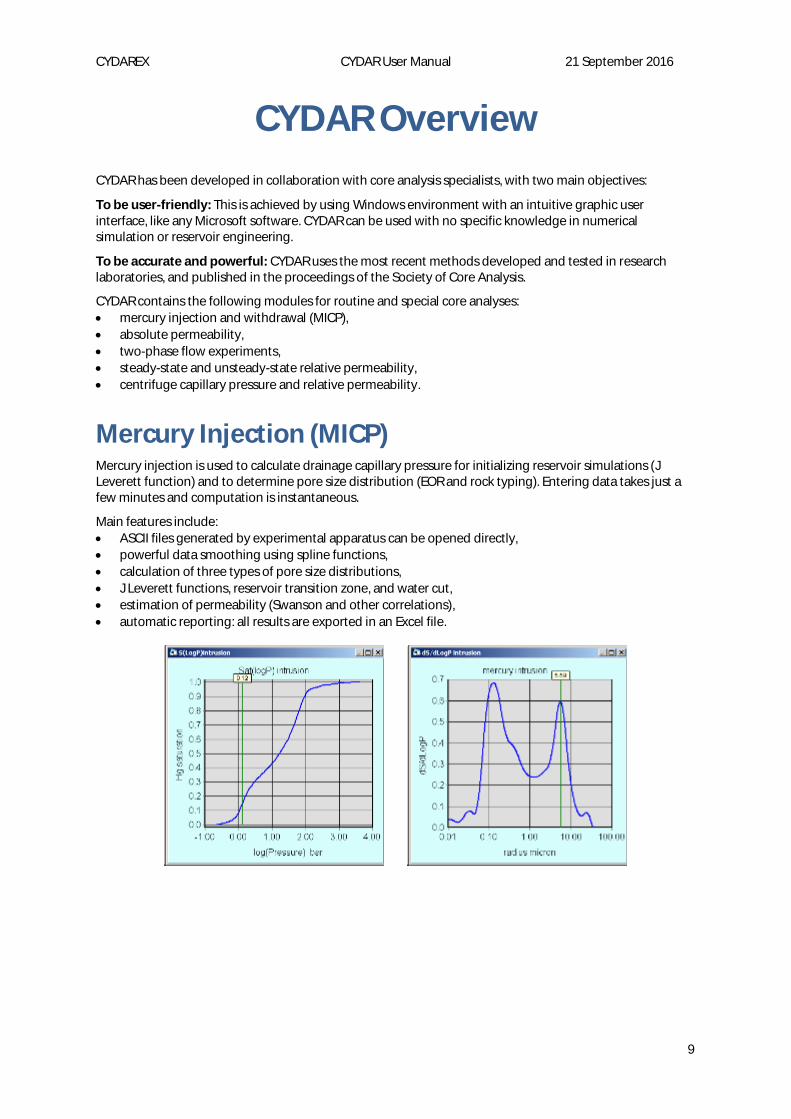
Mercury Injection (MICP) Mercury injection is used to calculate drainage capillary pressure for initializing reservoir simulations (J Leverett function) and to determine pore size distribution (EOR and rock typing). Entering data takes just a few minutes and computation is instantaneous.
Main features include:
ASCII files generated by experimental apparatus can be opened directly,
powerful data smoothing using spline functions,
calculation of three types of pore size distributions,
J Leverett functions, reservoir transition zone, and water cut,
estimation of permeability (Swanson and other correlations),
automatic reporting: all results are exported in an Excel file.
CYDAREX CYDAR User Manual 21 September 2016
10
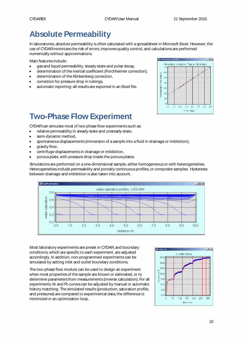
Absolute Permeability In laboratories, absolute permeability is often calculated with a spreadsheet in Microsoft Excel. However, the use of CYDAR minimizes the risk of errors, improves quality control, and calculations are performed numerically without approximations.
Main features include:
gas and liquid permeability, steady-state and pulse decay,
determination of the inertial coefficient (Forchheimer correction),
determination of the Klinkenberg correction,
correction for pressure drop in tubings,
automatic reporting: all results are exported in an Excel file.
Two-Phase Flow Experiment CYDAR can simulate most of two-phase flow experiments such as:
relative permeability in steady-state and unsteady-state,
semi-dynamic method,
spontaneous displacements (immersion of a sample into a fluid in drainage or imbibition),
gravity flow,
centrifuge displacements in drainage or imbibition,
porous plate, with pressure drop inside the porous plates.
Simulations are performed on a one-dimensional sample, either homogeneous or with heterogeneities. Heterogeneities include permeability and porosity continuous profiles, or composite samples. Hysteresis between drainage and imbibition is also taken into account.
Most laboratory experiments are preset in CYDAR, and boundary conditions, which are specific to each experiment, are adjusted accordingly. In addition, non-programmed experiments can be simulated by setting inlet and outlet boundary conditions.
The two-phase flow module can be used to design an experiment when most properties of the sample are known or estimated, or to determine parameters from measurements (inverse calculation). For all experiments, Kr and Pc curves can be adjusted by manual or automatic history matching. The simulated results (production, saturation profile, and pressures) are compared to experimental data; the difference is minimized in an optimization loop.

CYDAREX CYDAR User Manual 21 September 2016
11
Relative Permeability Determination of relative permeabilities Kr is one of the main objectives of special core analysis. It is now well recognized that numerical interpretations accounting for capillary effects are absolutely necessary.
Relative permeabilities can be determined by history matching of any transient experiment in steady-state (SS) and unsteady-state (USS) displacements, centrifuge, and semidynamic methods.
Main features include:
Kr models include Corey, modified Corey, and LET functions.
for unsteady-state displacements, analytical calculation using JBN, or Jones and Roszelles methods,
for steady-state displacements, analytical calculation assuming uniform profiles,
for SS and USS displacements, numerical simulation with capillary pressure, and determination of Kr using manual or automatic optimization (so-called history matching),
automatic reporting: all results are exported in an Excel file.
Centrifuge capillary pressure The centrifuge module converts the average saturation measured during the experiment to local saturation at the entrance of the sample, and additionally allows the evaluation of relative permeabilities.
Main features include:
displacement in drainage and imbibition,
choice of several interpretation methods such as Hassler Brunner, Forbes, and spline functions,
relative permeabilities determined by Hagoort method or multistep history matching,
automatic reporting: all results are exported in an Excel file.

CYDAREX CYDAR User Manual 21 September 2016
12
CYDAR main features All modules in CYDAR share the same features for data processing, graph and table displaying, and exporting results.
Windows environment
CYDAR is developed in Visual Basic, an object oriented language, which takes advantage of the familiar Windows environment. Some numerical calculations such as optimization loops use FORTRAN and its powerful IMSL library. However, all FORTRAN DLLs are controlled by CYDAR, and the user interacts only with the graphic user interface.
CYDAR does not require a high-performance computer, and runs perfectly on a laptop computer. CYDAR can be installed on any Windows operating systems including Windows XP, Vista, 7, 8, and 10, and does not require an Internet connection.
Data input
Several methods are used to input data. A small amount of data can be directly typed in; larger files can be cut and paste from Microsoft Excel or other applications. Some ASCII files generated by experimental apparatus can also be opened directly (like Autopore for mercury injection). CYDAR can also acquire data during experiments by reading pressure, temperature, and other parameters via USB connections.
For each parameter, the unit can be chosen in input, output, or for graph display.
Numerical calculation
Simulations are performed on a 1-D grid. The size of the grid and parameters for the numerical simulation can be adjusted for speed or accuracy. During numerical simulation and optimization, all variables (flow rates, effluent volumes, pressures, saturations...) are displayed dynamically; and the user can stop the simulation at any time to change parameters.
Exporting results
Graphs can be printed or copied into the clipboard in metafile or bitmap formats, and can be cut and paste into a Microsoft Word or Excel report. Graphs can also be saved as metafile, bitmap, or JPEG files. For each graph, the corresponding data set can be displayed as a table and copied into Microsoft Excel or other software by a cut and paste.
Data smoothing
Most experimental data are noisy and an efficient smoothing method is required for computation or comparison with simulated results for history matching. CYDAR offers several analytical functions for smoothing such as exponential, power law, and spline functions, the most general and powerful tool available.

CYDAREX CYDAR User Manual 21 September 2016
13
Graphical display
Variables can be displayed as a graph at the end or during simulations. Graph parameters (scale units, log scale, legends, symbols, colours...) can be adjusted.
Reporting
All results can be exported as an Excel file. Pre-formatted reports are available, and can be easily tailored by the user. The company logo can be added to the reports.
CYDAREX CYDAR User Manual 21 September 2016
14
CYDAR functionalities
This section describes some functions common to all modules and related to data handling and the graphic user interface.
Opening and saving projects The extension ".cyd" is
automatically added at the end of the project name.
Existing projects are opened following the standard Windows procedure, by double-clicking on the file. When opening a file for the first time, Windows may ask the user to select the appropriate program to connect as a CYDAR file. Use the navigator to find CYDAR.exe in the program files folder.
AutoSave Settings By default, a project is save every 10 min, but the delay can be reduced down to 1 minute. In order to avoid a crash during saving, the previous saved project is always kept. Consequently, there are always two saved projects with names xxxx_1 and xxxx_2. The saved project files can be saved when closing CYDAR. The user will be prompt to save a project when closing the application. To access the AutoSave settings, select settings AutoS .
The directory in which the project is saved is the system temporary folder and cannot be modified. The Open button will open the temporary folder in Windows Explorer (icon in the task bar, not on the desktop)
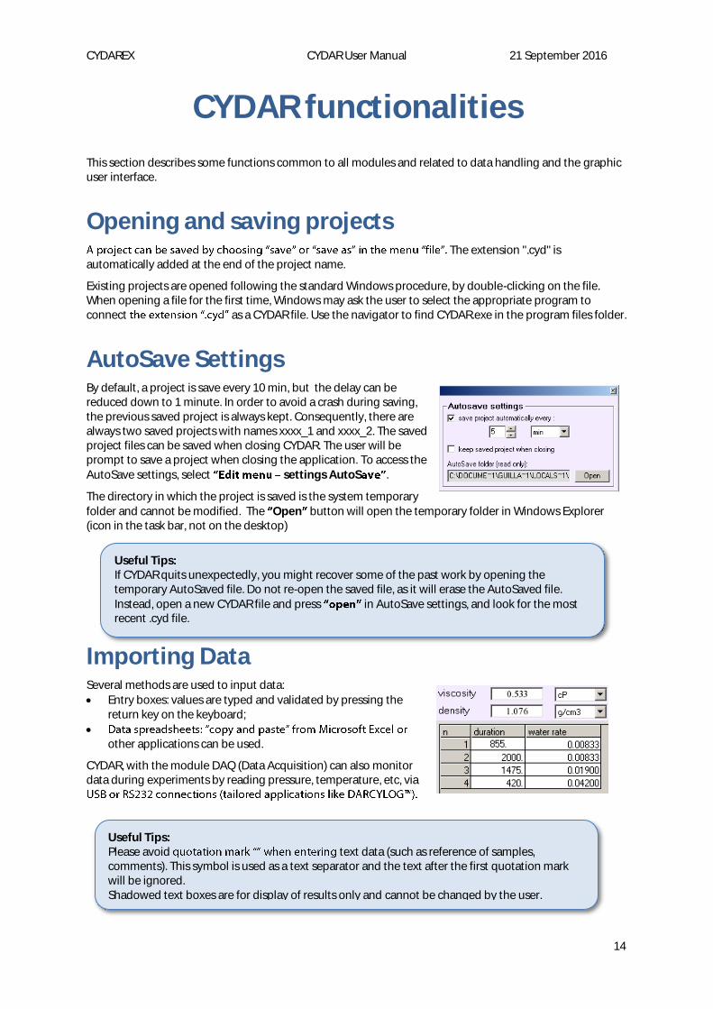
Importing Data Several methods are used to input data:
Entry boxes: values are typed and validated by pressing the return key on the keyboard;
other applications can be used.
CYDAR, with the module DAQ (Data Acquisition) can also monitor data during experiments by reading pressure, temperature, etc, via
Useful Tips: Please avoid text data (such as reference of samples, comments). This symbol is used as a text separator and the text after the first quotation mark will be ignored. Shadowed text boxes are for display of results only and cannot be changed by the user.
Useful Tips: If CYDAR quits unexpectedly, you might recover some of the past work by opening the temporary AutoSaved file. Do not re-open the saved file, as it will erase the AutoSaved file. Instead, open a new CYDAR file and press in AutoSave settings, and look for the most recent .cyd file.

CYDAREX CYDAR User Manual 21 September 2016
15
Reading ASCII files If required, CYDAR can open specific data files used by some equipments, such as the .rpt files provided by Autopore Mercury Injection device from Micromeritics Instrument Corporation. CYDAR can input data in the required format and units. An example is provided in MICP tutorials.
Loading data in CYDAR Most experimental data can be imported clicking on
, or (depending on the module). This opens a spreadsheet. Lines can be removed or inserted through the menu or the right click menu:
The left part of the spreadsheet has three frames:
Load raw data: the user can select the rows interval, data type, and units.
Noise filter: users can reduce noise by averaging data points over a specified number of points. When calculating average, the number of points furthest away from the average (end-points) can be removed. When using filtering, only filtered data are kept as raw data.
File reduction: users can reduce the number of data points by removing data points when a variable remains constant.
The specificities of the spreadsheets with the modules are described in the corresponding paragraphs.
Units All common units can be selected in combo boxes. Each data can have its own units: for instance, a sample can have its diameter expressed in inches and its length in cm. For calculation, all values are converted into the International Unit System, and results can be displayed in the selected unit.
For volume units, the Pore Volume unit is a dimensionless unit corresponding to the volume divided by the pore volume.
𝑡∗ =𝑉𝑖𝑛𝑗𝑒𝑐𝑡𝑒𝑑(𝑡)
𝑉𝑝𝑜𝑟𝑒, where t* is the dimensionless time, Vinjected(t) the total volume injected at time t, and Vpore the
Figure 1: a spreadsheet in CYDAR. Data are
CYDAREX CYDAR User Manual 21 September 2016
16
pore if it can be calculated. The dimensionless time is available for most experiment types in the TPF module.
is not available, data for the total volume for inlet sample need to be entered: once a simulation is run and the total volume for inlet sample has been
e a time unit option.
Number format To change the number format in a box, place the cursor on the number and select the "format" menu (or press Ctrl+F). In the displayed window, enter the format following Microsoft standard. For example:
0 for an integer (ex: 1343)
0.00 for a decimal number with a given number of digits (ex: 1343.45)
0.00E+0 for scientific format with two digits after the decimal point and 1 digit in the exponent (ex: 1343.45E+0)
mm/dd/yy hh:nn:ss for date (ex: 08/25/10 12:02:36).
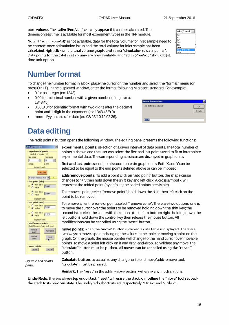
Data editing The "edit points" button opens the following window. The editing panel presents the following functions:
experimental points: selection of a given interval of data points. The total number of points is shown and the user can select the first and last points used to fit or interpolate experimental data. The corresponding abscissas are displayed in graph units.
first and last points: end points coordinates in graph units. Both X and Y can be selected to be equal to the end points defined above or can be imposed.
add/remove points: To add a point click on "add point" button, the shape cursor
changes to "+", then hold down the shift key and left click. A cross symbol will represent the added point (by default, the added points are visible).
To remove a point, select "remove point", hold down the shift then left click on the point to be removed.
To remove an entire zone of points select "remove zone". There are two options: one is to move the cursor over the points to be removed holding down the shift key; the second is to select the zone with the mouse (top left to bottom right, holding down the left button) hold down the control key then release the mouse button. All modifications can be cancelled using the "reset" button.
move points: two ways to move a point: changing the values in the table or moving a point on the graph. On the graph, the mouse pointer will change to the hand cursor over movable points. To move a point left click on it and drag-and-drop. To validate any move, the
" button.
Calculate button: to actualize any change, or to end move/add/remove tool,
Remark:
Undo-Redo: there is a five-
Figure 2: Edit points panel.

CYDAREX CYDAR User Manual 21 September 2016
17
Data smoothing Most experimental data are noisy and an efficient smoothing is needed for computation or history matching. Several analytical functions are available for smoothing, such as exponential or power law functions, but the most general and powerful tool is the spline functions.
Principle of data smoothing
Following a purpose of quality control, experimental data cannot be modified when they have been entered in CYDAR. However, the user can decide not to account for some experimental points which can be obviously erroneous. The user may also decide to add points needed for numerical simulations, such as end-points in relative permeability. The operation of adding and removing points is called "editing" and is accessible in most modules by selecting the button. Figure 3 shows an example where two end-function is detailed below.
An analytical function is then calculated to represent a continuous form of the discrete experimental values. The default case is a linear fit, which is a linear interpolation between each data point, represented as a pink curve on Figure 3. This analytical function is displayed with a number of points (100 by default) which can be
Figure 3: The pink solid line represents the analytical fit with a linear interpolation between all raw data points. The solid black line represents a linear interpolation between consecutive points, with two end-points added and 3 data points removed.
Curve fitting
CYDAR provides many analytical functions for smoothing and interpolation: -
exponential", "biExp Multi-Step", "parabolic", "modified hyperbolic", "Splines Multi-Step", "Splines Interpolation", "Akima Interpolation", and "Hermite Interpolation" (Figure 4).
These interpolation functions need to be used when optimizing Kr by points.
Interpolations (curve passes by all data points)
Linear: This corresponds to a linear interpolation between each data point.
Splines Interpolation: cubic spline interpolation with zero 2nd derivatives at end-points.
Akima Interpolation: cubic spline interpolation using Akima method to avoid wiggles in the interpolant.
added End points
Removed points
RAW DATA
Figure 4: Various functions available for fitting.
CYDAREX CYDAR User Manual 21 September 2016
18
Hermite Interpolation: Hermite cubic spline.
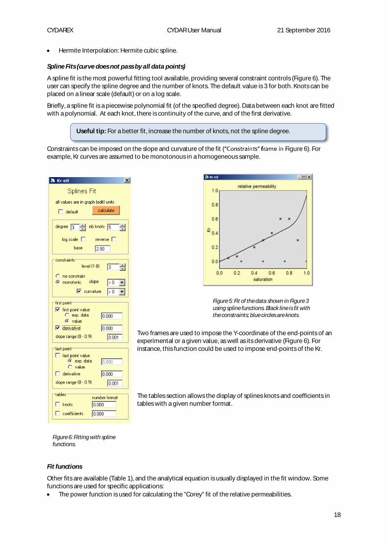
Spline Fits (curve does not pass by all data points)
A spline fit is the most powerful fitting tool available, providing several constraint controls (Figure 6). The user can specify the spline degree and the number of knots. The default value is 3 for both. Knots can be placed on a linear scale (default) or on a log scale.
Briefly, a spline fit is a piecewise polynomial fit (of the specified degree). Data between each knot are fitted with a polynomial. At each knot, there is continuity of the curve, and of the first derivative.
Constraints can be imposed on the slope and curvature of the fit ( Figure 6). For example, Kr curves are assumed to be monotonous in a homogeneous sample.
Two frames are used to impose the Y-coordinate of the end-points of an experimental or a given value, as well as its derivative (Figure 6). For instance, this function could be used to impose end-points of the Kr.
The tables section allows the display of splines knots and coefficients in tables with a given number format.
Fit functions
Other fits are available (Table 1), and the analytical equation is usually displayed in the fit window. Some functions are used for specific applications:
The power function is used for calculating the "Corey" fit of the relative permeabilities.
Figure 6: Fitting with spline functions.
Figure 5: Fit of the data shown in Figure 3 using spline functions. Black line is fit with the constraints; blue circles are knots.
Useful tip: For a better fit, increase the number of knots, not the spline degree.

CYDAREX CYDAR User Manual 21 September 2016
19
, or modified power law, is used to fit relative permeabilities, and corresponds to the equation:
Y =Ymax(a
2ax2a +
b
axa + Hx) with a = V-b-H and b = 2(1-H)-V+H.
The LET function is described in Reference 4, Lomeland et al., SCA, 2005, and is usually used for relative permeabilities.
The hyperbolic function is used for calculating the permeabilities from mercury injection by the Thomeer method13.
a) Power law
b) Modified power law
c) Parabolic
d) Modified hyperbolic
e) LogBeta
f) bi-exponential
g) LET function
Table 1: numerous fits are available.

CYDAREX CYDAR User Manual 21 September 2016
20
Multi-step fits
These fits can be used only in two-phase flow cases, when a specific variable called block times can be defined (see description of Two Phase Flow simulations).
Multi-Step Splines (Figure 7) allows using the CYDAR spline fit tool on each block time separately. The spline settings can is selected, the user must choose the blocks on the table by clicking on the left column. The corresponding area is highlighted on the graph with a yellow band as shown on Figure 8.
Figure 7: Multi-step splines fit
Figure 8: Multi-Step bi-exponential fit.
CYDAREX CYDAR User Manual 21 September 2016
21
Multi-Step bi-exponential fit uses the bi-exponential fit (Figure 8) on the selected block times.
Check boxes (numbered 1 to 5 on Figure 8): 1. Open a table with the parameters allowing the user to copy and paste the parameters to another
application. 2. Select/unselect all five parameters on all block times: Yo, Yinf, Alpha, Tau1 and Tau2. 3. Select/unselect a set of five parameters on one block time. 4. Select/unselect one parameter on all block times. 5. Select/unselect one parameter on one block time.
Buttons (Figure 8):
calculate of parameter. If no parameters are selected, the curve will be updated.
undo calculation e last calculation.
default o and Yinf from data points, Alpha = 0.5, Tau1 and Tau2 are the third of the block time interval.
accept
reset
Graphs CYDAR uses two types of graphs:
"Edit Points" graphs are used for editing data points (either experimental or calculated) with a default yellow background. These graphs are automatically open when calling editing or fitting functions.
"XY-graphs" are for displaying input or output data; they have a default blue background. These graphs can be opened with the "view" menu of the main Window.
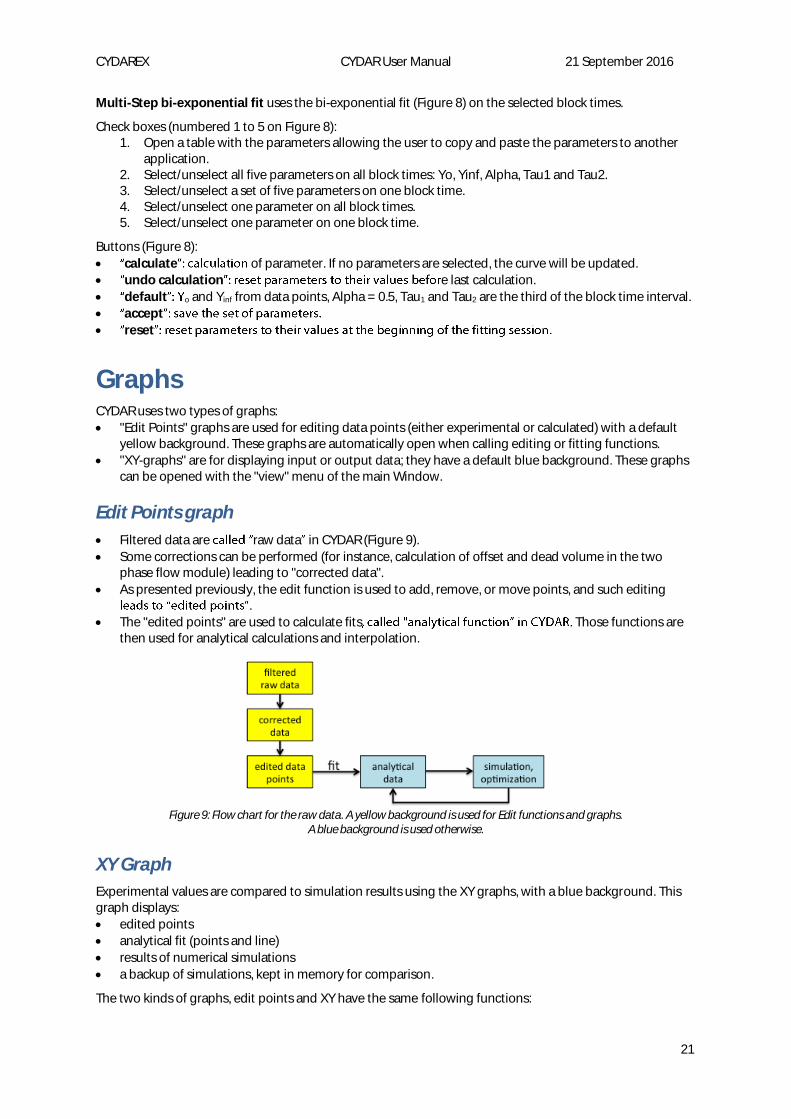
Edit Points graph
Filtered data are raw data in CYDAR (Figure 9).
Some corrections can be performed (for instance, calculation of offset and dead volume in the two phase flow module) leading to "corrected data".
As presented previously, the edit function is used to add, remove, or move points, and such editing .
The "edited points" are used to calculate fits . Those functions are then used for analytical calculations and interpolation.
Figure 9: Flow chart for the raw data. A yellow background is used for Edit functions and graphs.
A blue background is used otherwise.
XY Graph
Experimental values are compared to simulation results using the XY graphs, with a blue background. This graph displays:
edited points
analytical fit (points and line)
results of numerical simulations
a backup of simulations, kept in memory for comparison.
The two kinds of graphs, edit points and XY have the same following functions:

CYDAREX CYDAR User Manual 21 September 2016
22
Scaling up and scaling down a graph selection
To scale up a part of graph, select the corresponding section with the mouse (top left to bottom right) holding down the left button (Figure 10a; result shown in Figure 10b). To undo, select a section of the graph with no data, holding down the left button from the bottom right to the top left (Figure 10b; result shown in Figure 10c).
Figure 10: Zooming and unzooming on a graph window.
Moving the display zone
On a graph window, the user can move the display zone by pointing on the graph, holding down the right button, and moving the pointer. To go back to the normal view, the procedure is the same than to unzoom.
Editing a graph
Graph display parameters can be changed by double-clicking on the graph window or clicking on the axes. The Graph Edition panel (Figure 11) allows modification of most parameters, such as scale units, log scale, legends, symbols, colors, etc...
Figure 11: Graph edition panel.
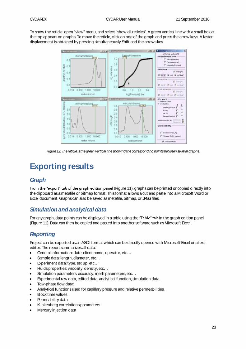
Reticles
A reticle (a vertical moving line) can be used to display corresponding points between different graphs, for instance pore radius and capillary pressure (Figure 12).
CYDAREX CYDAR User Manual 21 September 2016
23
To show the reticle, open "view" menu, and select "show all reticles". A green vertical line with a small box at the top appears on graphs. To move the reticle, click on one of the graph and press the arrow keys. A faster displacement is obtained by pressing simultaneously Shift and the arrows key.
Figure 12: The reticle is the green vertical line showing the corresponding points between several graphs.
Exporting results
Graph
Figure 11), graphs can be printed or copied directly into the clipboard as a metafile or bitmap format. This format allows a cut and paste into a Microsoft Word or Excel document. Graphs can also be saved as metafile, bitmap, or JPEG files.
Simulation and analytical data
For any graph, data points can be displayed in a table using the in the graph edition panel (Figure 11). Data can then be copied and pasted into another software such as Microsoft Excel.
Reporting
Project can be exported as an ASCII format which can be directly opened with Microsoft Excel or a text editor. The report summarizes all data:
General information: date, client name, operator, etc
Sample data: length, diameter, etc
Experiment data: type, set up, etc
Fluids properties: viscosity, density, etc
Simulation parameters: accuracy, mesh parameters, etc
Experimental raw data, edited data, analytical function, simulation data
Tow-phase flow data:
Analytical functions used for capillary pressure and relative permeabilities.
Block time values
Permeability data:
Klinkenberg correlations parameters
Mercury injection data
CYDAREX CYDAR User Manual 21 September 2016
24
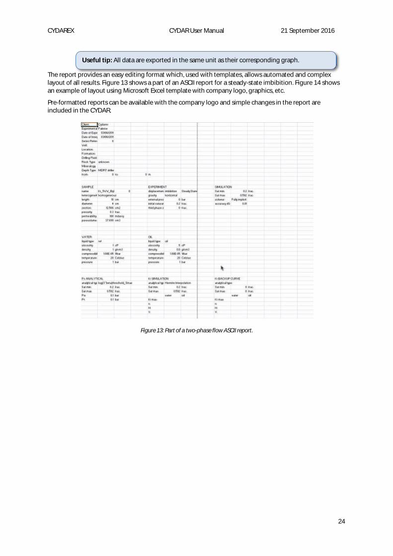
The report provides an easy editing format which, used with templates, allows automated and complex layout of all results. Figure 13 shows a part of an ASCII report for a steady-state imbibition. Figure 14 shows an example of layout using Microsoft Excel template with company logo, graphics, etc.
Pre-formatted reports can be available with the company logo and simple changes in the report are included in the CYDAR.
Figure 13: Part of a two-phase flow ASCII report.
Useful tip: All data are exported in the same unit as their corresponding graph.

CYDAREX CYDAR User Manual 21 September 2016
25
Figure 14: Example of a more complex layout using a template.
Copying a graph or a frame
Select the graph or the frame and press Cedit menu. Then copy in Microsoft Word, Excel, or any other software.

CYDAREX CYDAR User Manual 21 September 2016
26
New Project Window
Figure 15: CYDAR new project window.
Mercury injection: interpretation of experiments with calculation of the dS/dP, psd and ds/dLogP curves.
Permeability: absolute permeability calculation for gas and liquid, steady state and transient experiments, using Klinkenberg correction, inertial effect, and correction of pressure drop in tubings.
Two Phase flow frame:
One Fluid Injected: launches the Two Phase Flow module for unsteady state experiments, allowing analytical calculation of the Kr.
Two Fluid Injected: launches the Two Phase Flow module for steady state experiments.
Centrifuge Kr Pc: launches the Two Phase Flow module for centrifugation experiments with calculation of the locale Pc curve from experimental data and the Hagoort Kr.
Two phase flow: Simulation of a large panel of experiments, from gravity flow to unsteady state experiments.
Data Acquisition frame: data acquisition from specific experimental set-up. These modules are optional, and may not be activated on your version.
DataBase: possibility to create a database with different kind of fields, such as rock type, experiment type, client, operator, date. This module is under development and may not be activated on your version.
Curve fitting: access to CYDAR curve fitting tools.

CYDAREX CYDAR User Manual 21 September 2016
27
Mercury Injection Module
Mercury injection is used to calculate drainage capillary pressure for initializing reservoir simulations (Leverett J function) and to determine pore size distribution (EOR and rock typing).
Main features:
direct opening of the ASCII file generated by the experimental apparatus,
powerful data smoothing using spline functions,
calculation of 3 types of pore size distributions (PSDs),
calculation of Pc curves for reservoir fluids and saturations in transition zones,
calculation of water cut in transition zone when producing the well,
permeability estimation using Purcell, Swanson11, and Thomeer13 methods,
automated reporting.
Mercury main window Mercury injection he Mercury main window (Figure 16). This window allows loading
data, fitting curves, calculating PSD (Pore Size Distribution), and more.
Data frame: Informationand all information regarding the sample.
: The list box allows selection of the type of input, either from an ASCII file or from a data file from an apparatus (such as Micromeritics
: Specifies which parts of the data corresponds to the first intrusion, to the extrusion, and to the second intrusion (detailed below).
Parameters frame:
the experimental conditions; these vales are used for pore size
standard conditions. The total volume (or bulk volume) is optional and used only to calculate porosity.
Displacement Frame: Fit using linear or splines functions to one of the displacements: intrusion, extrusion, or 2nd intrusion.
Results frame:
r at maximumcorresponding to the maximum of ds/dLogP. Porosity is calculated from the volume of mercury injected (pore
Capillary pressureLeverett function. It is used to calculate a capillary pressure curve with a different couple of fluids, and the profile of saturation in reservoir transition zones.
permeabilityfrom the mercury Pc curve (Purcell, Swanson11
Figure 16: Mercury main window
CYDAREX CYDAR User Manual 21 September 2016
28
Report frame:
Common to all options: general information, mercury and sample properties, experimental data;
meabilit 11 and Thomeer parameters and data.
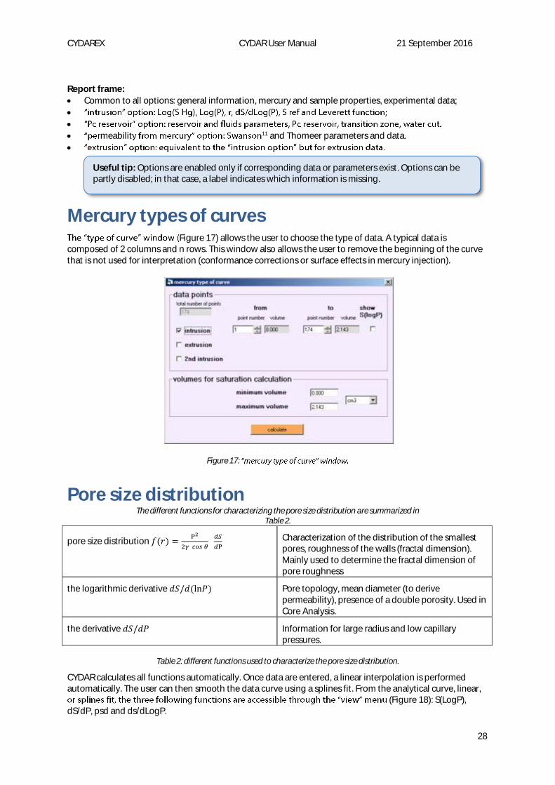
Mercury types of curves Figure 17) allows the user to choose the type of data. A typical data is
composed of 2 columns and n rows. This window also allows the user to remove the beginning of the curve that is not used for interpretation (conformance corrections or surface effects in mercury injection).
Figure 17:
Pore size distribution The different functions for characterizing the pore size distribution are summarized in
Table 2.
pore size distribution 𝑓(𝑟) =P2
2𝛾 𝑐𝑜𝑠 𝜃
𝑑𝑆
𝑑P Characterization of the distribution of the smallest
pores, roughness of the walls (fractal dimension). Mainly used to determine the fractal dimension of pore roughness
the logarithmic derivative 𝑑𝑆/𝑑(ln𝑃) Pore topology, mean diameter (to derive permeability), presence of a double porosity. Used in Core Analysis.
the derivative 𝑑𝑆/𝑑𝑃 Information for large radius and low capillary pressures.
Table 2: different functions used to characterize the pore size distribution.
CYDAR calculates all functions automatically. Once data are entered, a linear interpolation is performed automatically. The user can then smooth the data curve using a splines fit. From the analytical curve, linear,
(Figure 18): S(LogP), dS/dP, psd and ds/dLogP.
Useful tip: Options are enabled only if corresponding data or parameters exist. Options can be partly disabled; in that case, a label indicates which information is missing.

CYDAREX CYDAR User Manual 21 September 2016
29
In the view window (right side of Figure 18 nd
(Figure 17).
Figure 18:
Permeability calculation
Thompson, Swanson11 and Thomeer13 relationships are implemented. The porosity value is necessary for all models.
Figure 19: Estimation of permeability from mercury injection.
Models based on formation factor:
Φ−2, otherwise the formation factor must be specified. Permeabilities are calculated automatically.
Pc interval:
The range selected is useful in case of double porosity to adjust the interval of pressure for permeability determination.
Swanson:
The 3 brine permeability values correspond to the experimental relationships given in Swanson publication (between permeabilities and mercury capillary
Journal of Petroleum Technology, December, 2498-2504, 1981) for sandstones, carbonates, and an average over all the samples.
is the gas permeability relationship
Checking displays the Swanson graph with Swanson point and tangent (Figure 20).
CYDAREX CYDAR User Manual 21 September 2016
30
Thomeer:
The parameters correspond to the original publication. The procedure is the following:
Fit Table 1d)) for fitting the Log(Pc) vs. Log(SHg) curve. It is recommended to start with the first guess then to optimized parameters a, b and c. The Accept button keeps parameter values. Alpha is fixed to 1.
The calculate button determines Thomeer parameters and the permeability.
Generally the result depends on the Pc interval chosen for the fit of the hyperbola.
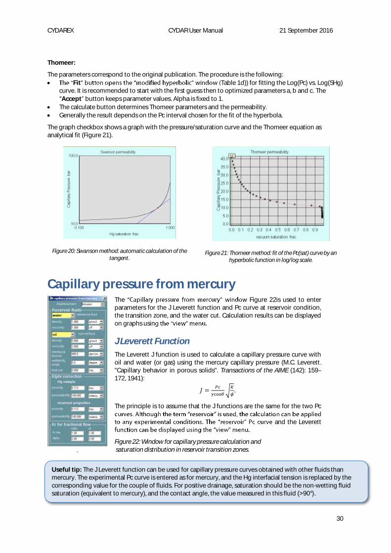
The graph checkbox shows a graph with the pressure/saturation curve and the Thomeer equation as analytical fit (Figure 21).
Figure 20: Swanson method: automatic calculation of the tangent.
Figure 21: Thomeer method: fit of the Pc(sat) curve by an hyperbolic function in log/log scale.
Capillary pressure from mercury
.
The Figure 22is used to enter parameters for the J Leverett function and Pc curve at reservoir condition, the transition zone, and the water cut. Calculation results can be displayed on graphs usin
J Leverett Function
The Leverett J function is used to calculate a capillary pressure curve with oil and water (or gas) using the mercury capillary pressure (M.C. Leverett. "Capillary behavior in porous solids". Transactions of the AIME (142): 159172, 1941):
𝐽 =𝑃𝑐
𝛾cos𝜃√
𝐾
𝜙.
The principle is to assume that the J functions are the same for the two Pc
and the Leverett
Figure 22: Window for capillary pressure calculation and saturation distribution in reservoir transition zones.
Useful tip: The J Leverett function can be used for capillary pressure curves obtained with other fluids than mercury. The experimental Pc curve is entered as for mercury, and the Hg interfacial tension is replaced by the corresponding value for the couple of fluids. For positive drainage, saturation should be the non-wetting fluid saturation (equivalent to mercury), and the contact angle, the value measured in this fluid (>90°).
CYDAREX CYDAR User Manual 21 September 2016
31
Transition zones
Saturation in the transition zones is derived from the balance between gravity and capillary forces:
𝑃𝑐 = 𝑃𝑜𝑖𝑙 − 𝑃𝑤 = (𝜌𝑤 − 𝜌𝑜𝑖𝑙)𝑔ℎ.
In addition to the parameters used in the J functions, this calculation requires the reservoir oil and water densities.
Water cut
This function is used to estimate the production of the well at a given position in the transition zone. The top of the transition zone produces 100% oil and the bottom only water. The water fractional flow (also called
𝑓𝑤 =𝑄𝑤
𝑄𝑤+𝑄𝑜=
𝐾𝑟𝑤/𝜇𝑤
𝐾𝑟𝑤/𝜇𝑤+𝐾𝑟𝑜/𝜇𝑜.
Fluid viscosities are entered and relative permeabilities are calculated using the approximation of a Corey function with parameters defined in the window.
Tutorial files
Tutorial_Hg_SampleA
This example uses an ASCII file generated by an AUTOPORE apparatus (Tutorial_Hg_SampleA.rpt) and
In order to calculate the porosity, the user must enter the total volume of 6.5 cc.
Tutorial_Hg_Brauvillier
This example uses an ASCII file from the Microsoft
In order to calculate the porosity, the user must enter the total volume of 7.733 cc.

CYDAREX CYDAR User Manual 21 September 2016
32
Permeability Module
In most laboratories, absolute permeabilities are generally calculated with a Microsoft Excel spreadsheet using permanent flow experiments. Using CYDAR minimizes the risk of errors, improves the quality control, and allows the permeability determination from transient flow.
CYDAR includes the following options:
Steady state and transient flow experiments,
Determination of inertial coefficient (Forchheimer correction),
Determination of Klinkenberg correction,
Transient flow experiments, with the possibility to take into account experimental setup dilatation due to pressure,
Automated reporting to export results in an Excel file.
Permeability main window Experiment frame: Transient : pulse decay experiments. Steady-state : permanent flow experiments.
Liquid : constant compressibility (transient). Gas
Data frame: Information : common to all modules, allows entering information regarding the
sample and experience. None of this information is used for calculation. Sample : dimensions and porosity of a cylindrical sample. Fluid : fluid properties window. Data points : input data spreadsheet, see below.
Klinkenberg correlations button displays a panel to estimate Klinkenberg Klinkenberg correlations
Calculate permeability determination of permeability with four possible correc Calculate permeability: steady-state Permeability pulse
Graphs view
Sample and fluid properties The sample is assumed to be cylindrical. In steady-state, the porosity is optional, and is only used in calculating the Reynolds number. In addition to the length, the user needs to enter one of the following: the diameter, the section, or the pore volume if the porosity is known (Figure 24). Because the porosity can be optimized in the transient module, its input is on the calculation window (Figure 23). Figure 25 shows the fluid properties windows.
Figure 23: Permeability Main Window.

CYDAREX CYDAR User Manual 21 September 2016
33
Figure 24: Sample window.
Figure 25: .
Klinkenberg correlations
This window allows the Klinkenberg coefficient calculation from well-known correlations. The values are only output, they are not used in CYDAR calculation.
automatic Kg and P values ability to the permeability set
Figure 23) and the absolute pressure.
The automatic absolute pressure is: In a steady-state experiment, the average between the maximum inlet pressure and the minimum outlet pressure. In a transient experiment, the average of the averages between maximum and minimum of each data. The different models used are described in the corresponding journal articles, given in the Reference section below. For instance, the Jones & Owens[15] correction uses the following equation:
𝑏 = 0.86 𝐾𝑔∞−0.33
Steady-state experiment
Data points steady-state
on Figure 23 opens a spreadsheet (Figure 27 and Figure 28). Data can be added by copy/paste from other programs such as Microsoft Excel, CYDAR spreadsheet, a text file, or manually typed.
Figure 26: Klinkenberg correlations window.
CYDAREX CYDAR User Manual 21 September 2016
34
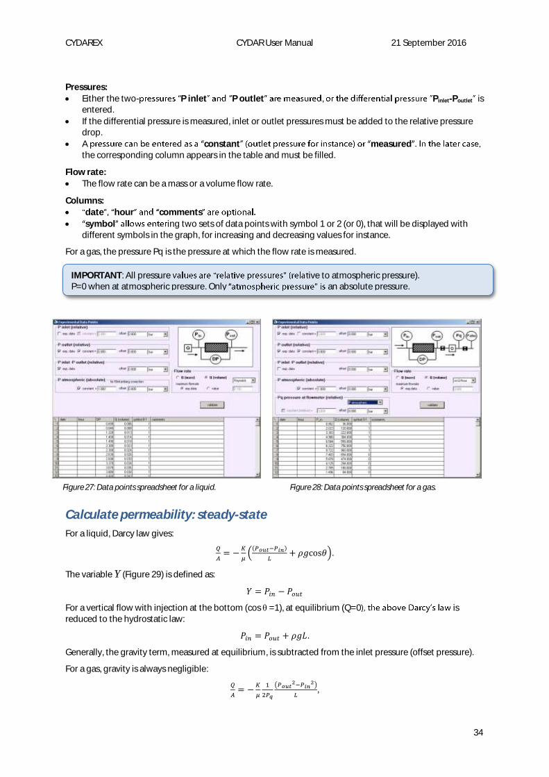
Pressures:
Either the two- P inlet P outlet , Pinlet-Poutlet is entered.
If the differential pressure is measured, inlet or outlet pressures must be added to the relative pressure drop.
A constant measuredthe corresponding column appears in the table and must be filled.
Flow rate:
The flow rate can be a mass or a volume flow rate.
Columns:
date hour comments
symbol ing two sets of data points with symbol 1 or 2 (or 0), that will be displayed with different symbols in the graph, for increasing and decreasing values for instance.
For a gas, the pressure Pq is the pressure at which the flow rate is measured.
Calculate permeability: steady-state
For a liquid, Darcy law gives:
𝑄
𝐴= −
𝐾
𝜇(
(𝑃𝑜𝑢𝑡−𝑃𝑖𝑛)
𝐿+ 𝜌𝑔cos𝜃).
The variable Y (Figure 29) is defined as:
𝑌 = 𝑃𝑖𝑛 − 𝑃𝑜𝑢𝑡
For a vertical flow with injection at the bottom (cos θ =1), at equilibrium (Q=0 is reduced to the hydrostatic law:
𝑃𝑖𝑛 = 𝑃𝑜𝑢𝑡 + 𝜌𝑔𝐿.
Generally, the gravity term, measured at equilibrium, is subtracted from the inlet pressure (offset pressure).
For a gas, gravity is always negligible:
𝑄
𝐴= −
𝐾
𝜇
1
2𝑃𝑞
(𝑃𝑜𝑢𝑡2−𝑃𝑖𝑛
2)
𝐿,
IMPORTANT: All pressure ive to atmospheric pressure). P=0 when at atmospheric pressure. Only an absolute pressure.
Figure 27: Data points spreadsheet for a liquid. Figure 28: Data points spreadsheet for a gas.
CYDAREX CYDAR User Manual 21 September 2016
35
where 𝑄 is the flow rate measured at the pressure 𝑃𝑞. The variable is defined as:
𝑌 =𝑃𝑖𝑛
2−𝑃𝑜𝑢𝑡2
2𝑃𝑞.
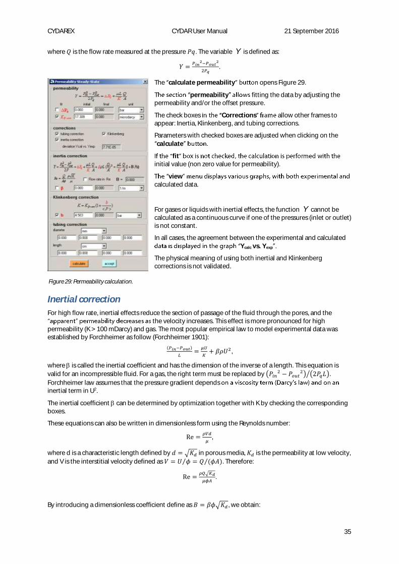
The calculate permeability opens Figure 29.
T permeability fitting the data by adjusting the permeability and/or the offset pressure.
The check boxes Corrections allow other frames to appear: Inertia, Klinkenberg, and tubing corrections.
Parameters with checked boxes are adjusted when clicking on the
calculate
fitinitial value (non zero value for permeability).
viewcalculated data.
For gases or liquids with inertial effects, the function cannot be calculated as a continuous curve if one of the pressures (inlet or outlet) is not constant.
In all cases, the agreement between the experimental and calculated Ycalc vs. Yexp .
The physical meaning of using both inertial and Klinkenberg corrections is not validated.
Inertial correction
For high flow rate, inertial effects reduce the section of passage of the fluid through the pores, and the the velocity increases. This effect is more pronounced for high
permeability (K > 100 mDarcy) and gas. The most popular empirical law to model experimental data was established by Forchheimer as follow (Forchheimer 1901):
(𝑃𝑖𝑛−𝑃𝑜𝑢𝑡)
𝐿=
𝜇𝑈
𝐾+ 𝛽𝜌𝑈2,
where is called the inertial coefficient and has the dimension of the inverse of a length. This equation is
valid for an incompressible fluid. For a gas, the right term must be replaced by (𝑃𝑖𝑛2 − 𝑃𝑜𝑢𝑡
2) (2𝑃𝑞𝐿)⁄ .
Forchheimer law assumes that the pressure gradient depends inertial term in U2.
The inertial coefficient can be determined by optimization together with K by checking the corresponding boxes.
These equations can also be written in dimensionless form using the Reynolds number:
Re =𝜌𝑉𝑑
𝜇,
where d is a characteristic length defined by 𝑑 = √𝐾𝑑 in porous media, 𝐾𝑑 is the permeability at low velocity,
and V is the interstitial velocity defined as 𝑉 = 𝑈 𝜙⁄ = 𝑄 (𝜙𝐴)⁄ . Therefore:
Re =𝜌𝑄√𝐾𝑑
𝜇𝜙𝐴.
By introducing a dimensionless coefficient define as 𝐵 = 𝛽𝜙√𝐾𝑑 , we obtain:
Y
Y
Figure 29: Permeability calculation.

CYDAREX CYDAR User Manual 21 September 2016
36
(𝑃𝑖𝑛−𝑃𝑜𝑢𝑡)
𝐿=
𝜇𝑈
𝐾(1 + 𝐵Re).
Typically the inertial effect becomes significant when Re ≥ 1. On the graph, the flow rate can be displayed in the unit of Reynolds numbers, to verify if the inertial correction is justified.
Klinkenberg correction
The principle of the calculation is a non-linear optimization on all points to determine simultaneously the KL that corresponds to the limit of infinite pressure, and the Klinkenberg parameter b. It
is recommended to set the offset Δ𝑃0to zero for the Klinkenberg calculation:
𝑄
𝐴= −
𝐾𝐺
𝜇
1
2𝑃𝑞
(𝑃𝑜𝑢𝑡2−𝑃𝑖𝑛
2)
𝐿,
with the gas permeability defined as:
𝐾𝐺 = KL (1 +b
⟨𝑃⟩).
The optimization is performed using a Levenberg-Marquardt method from the IMSL Fortran Library. Due to the method of calculation, all the calculated points are always exactly on the line K(1/<P>) on the Klinkenberg graph. The Ycalc vs. Yexp to control the fit accuracy.
Tubing correction
tubing correction , and subtracts this pressure to the measured pressure. This effect is noticeable with tubings of small diameters. The window allows entering four different tubing with diameter and length, mounted in series.
Transient experiment
Data points transient / unsteady state
Figure 30: Data points transient window.
IMPORTANT: All pressures are relative to the atmospheric pressure, except the atmospheric pressure itself, which is absolute.
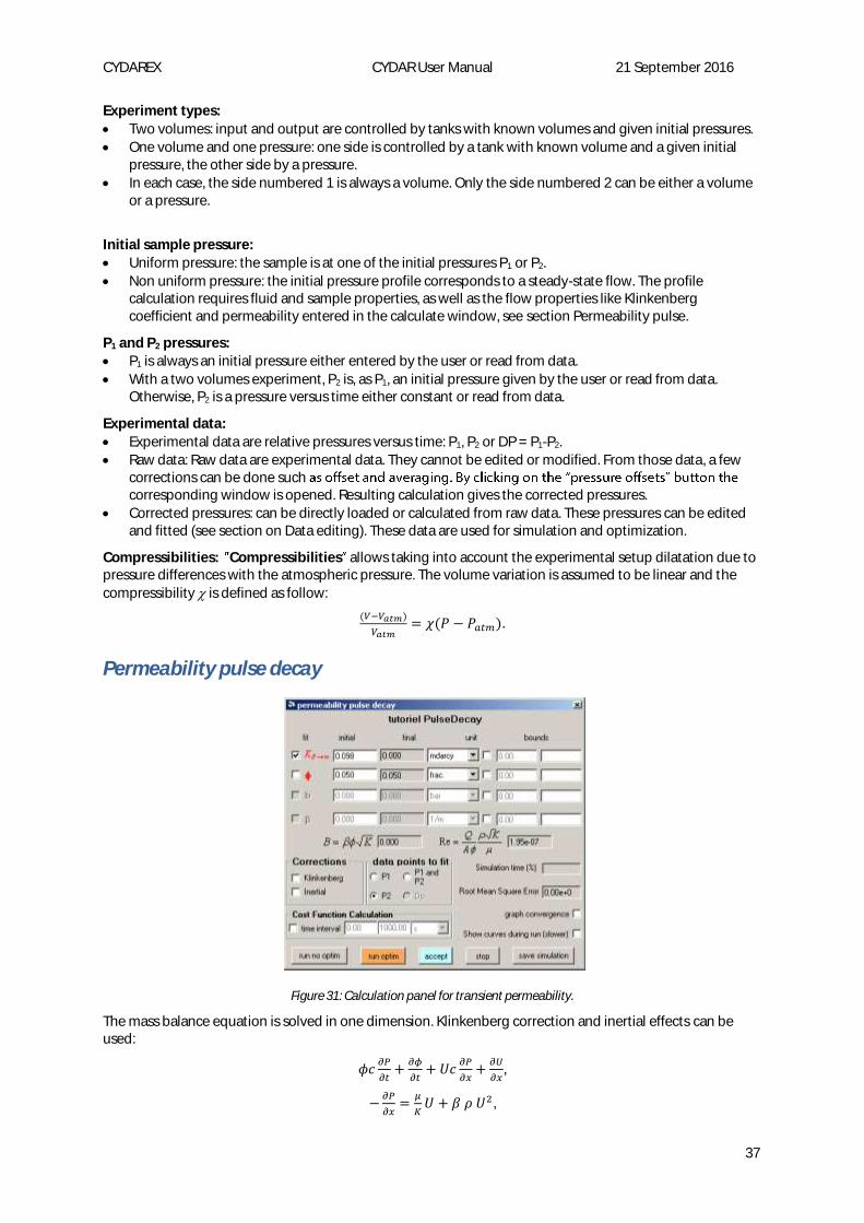
CYDAREX CYDAR User Manual 21 September 2016
37
Experiment types:
Two volumes: input and output are controlled by tanks with known volumes and given initial pressures.
One volume and one pressure: one side is controlled by a tank with known volume and a given initial pressure, the other side by a pressure.
In each case, the side numbered 1 is always a volume. Only the side numbered 2 can be either a volume or a pressure.
Initial sample pressure:
Uniform pressure: the sample is at one of the initial pressures P1 or P2.
Non uniform pressure: the initial pressure profile corresponds to a steady-state flow. The profile calculation requires fluid and sample properties, as well as the flow properties like Klinkenberg coefficient and permeability entered in the calculate window, see section Permeability pulse.
P1 and P2 pressures:
P1 is always an initial pressure either entered by the user or read from data.
With a two volumes experiment, P2 is, as P1, an initial pressure given by the user or read from data. Otherwise, P2 is a pressure versus time either constant or read from data.
Experimental data:
Experimental data are relative pressures versus time: P1, P2 or DP = P1-P2.
Raw data: Raw data are experimental data. They cannot be edited or modified. From those data, a few corrections can be done such corresponding window is opened. Resulting calculation gives the corrected pressures.
Corrected pressures: can be directly loaded or calculated from raw data. These pressures can be edited and fitted (see section on Data editing). These data are used for simulation and optimization.
Compressibilities: Compressibilities allows taking into account the experimental setup dilatation due to pressure differences with the atmospheric pressure. The volume variation is assumed to be linear and the
compressibility is defined as follow:
(𝑉−𝑉𝑎𝑡𝑚)
𝑉𝑎𝑡𝑚= 𝜒(𝑃 − 𝑃𝑎𝑡𝑚).
Permeability pulse decay
Figure 31: Calculation panel for transient permeability.
The mass balance equation is solved in one dimension. Klinkenberg correction and inertial effects can be used:
𝜙𝑐∂𝑃
∂𝑡+
∂𝜙
∂𝑡+ 𝑈𝑐
∂𝑃
∂𝑥+
∂𝑈
∂𝑥,
−∂𝑃
∂𝑥=
𝜇
𝐾𝑈 + 𝛽 𝜌 𝑈2,

CYDAREX CYDAR User Manual 21 September 2016
38
𝐾 = 𝐾𝐿 (1 +𝑏
⟨P⟩).
The numerical scheme is implicit and the system is solved by a Newton-Raphson algorithm. The cost function is calculated with P1, P2, both, or DP=P1-P2 in Figure 31).
Buttons:
run no optim s one simulation without any optimization.
run optim s optimization on selected parameters: permeability, porosity, Klinkenberg coefficient and/or inertial coefficient.
accept s optimized values. This action erases the first guess values.
stop s simulation and optimization.
Back up curve
The user can give bounds to each parameter using the corresponding check boxes.
Parameter menu transient:
In transient type experiment, an additional menu is enabled to access numerical parameters (Figure 32):
Duration : duration of the simulation. Simulation : simulation accuracy on pressure (adimensional).
Mesh : grid number. Uniform grid : if not selected, the mesh cells grow progressively from the
outlets to the sample center symmetrically as follow: dxi = rdxi-1. The user gives r -
Display points number: sets the number of points of the simulation curve displayed on graphs.
smallest dx a read-only value giving the smallest dx existing in the mesh.
Cost function calculation : By default, the cost function is calculated over the entire time interval defined above on a linear time scale. However, the user can define a time interval and a time log scale.
Tutorial files
Tutorial_Perm_Klinkenberg
Data of the steady-state Gas tutorial are in the Microsoft E
Tutorial_Perm_Inertial
Data of the steady-state liquid tutorial are in the Microsoft Eco
Figure 32: Numerical parameter window for absolute permeability calculation in transient flow.
Useful Tips: Although permeability, porosity, Klinkenberg, and inertial coefficients can be optimized all together, it is recommended to perform optimization one parameter at a time.

CYDAREX CYDAR User Manual 21 September 2016
39
Tutorial_PERM_Pulse_decay_Analytical
Data of the transient gas tutorial are in the Microsoft Excel file
CYDAREX CYDAR User Manual March 2013
Two-phase Flow Module
Immiscible flows (two-phase flow, noted TPF) are the most important part of core analysis. The two-phase flow modules of CYDAR allow two complementary approaches:
Direct simulation: To simulate an experiment before running it, to determine the optimal experimental parameters (duration, injection flow rate or pressure). In this approach, the parameters such as relative permeabilities (Kr) and capillary pressure (Pc) are assumed to be known.
Parameter estimation: To use experimental data to determine unknown parameters, mainly Kr and Pc. This can be done by using analytical approaches, numerical optimization, or history matching.
The two-phase flow functions are described in the following sections of this manual and organized as follows:
TPF direct simulation: how to enter the parameters to simulate any kind of displacement, injection of one or two fluids, porous plate, centrifuge, etc.
TPF optimization: description of the principle of the optimization used to determine one or several parameters from an experiment
In addition, CYDAR allows specific calculations for standard procedures to determine Kr and Pc:
Unsteady-state experiments for Kr determination. One fluid is injected and the transient productions and pressures are used to determine Kr. Historically, only one step was used and interpreted with analytical equations assuming that capillary pressure was negligible. This method is available and called JBN (and Jones and Roszelle). However, a more accurate method is now preferred, based on a multi-step displacement and using numerical optimization. This method can also lead to the determination of the capillary pressure curve during the same experiment.
Steady-state experiments. This method is based on the simultaneous injection of two fluids at various ratios. As a first stage, an analytical calculation gives an estimate of the Kr curves. Then an optimization with the experimental data is possible to improve result.
Centrifugation. Several results are available from centrifuge experiments. The first is the determination n data, using Forbes and spline methods.
The centrifuge also allows determination of the Kr, either in a single step (single speed) or multispeed experiments, using numerical optimization
Porous plate. CYDAR is mainly used with simulation to optimize the duration of the various steps of pressures.
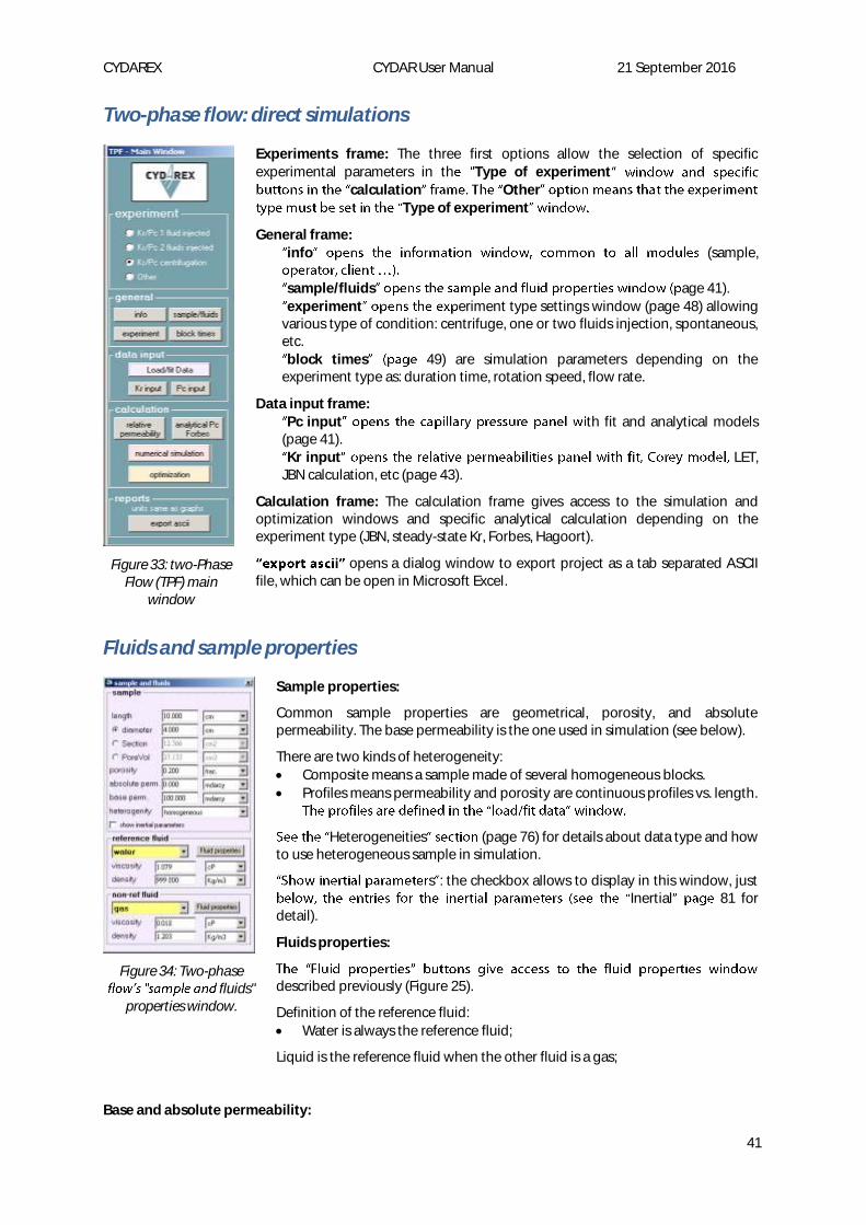
CYDAREX CYDAR User Manual 21 September 2016
41
Two-phase flow: direct simulations
Figure 33: two-Phase Flow (TPF) main
window
Experiments frame: The three first options allow the selection of specific experimental parameters in th Type of experiment
calculation OtherType of experiment
General frame: info (sample,
sample/fluids age 41).
experiment eriment type settings window (page 48) allowing various type of condition: centrifuge, one or two fluids injection, spontaneous, etc. block times 49) are simulation parameters depending on the
experiment type as: duration time, rotation speed, flow rate.
Data input frame: Pc input th fit and analytical models
(page 41). Kr input LET,
JBN calculation, etc (page 43).
Calculation frame: The calculation frame gives access to the simulation and optimization windows and specific analytical calculation depending on the experiment type (JBN, steady-state Kr, Forbes, Hagoort).
opens a dialog window to export project as a tab separated ASCII file, which can be open in Microsoft Excel.
Fluids and sample properties
Figure 34: Two-phase fluids"
properties window.
Sample properties:
Common sample properties are geometrical, porosity, and absolute permeability. The base permeability is the one used in simulation (see below).
There are two kinds of heterogeneity:
Composite means a sample made of several homogeneous blocks.
Profiles means permeability and porosity are continuous profiles vs. length.
Heterogeneities (page 76) for details about data type and how to use heterogeneous sample in simulation.
s : the checkbox allows to display in this window, just Inertial 81 for
detail).
Fluids properties:
described previously (Figure 25).
Definition of the reference fluid:
Water is always the reference fluid;
Liquid is the reference fluid when the other fluid is a gas;
Base and absolute permeability:
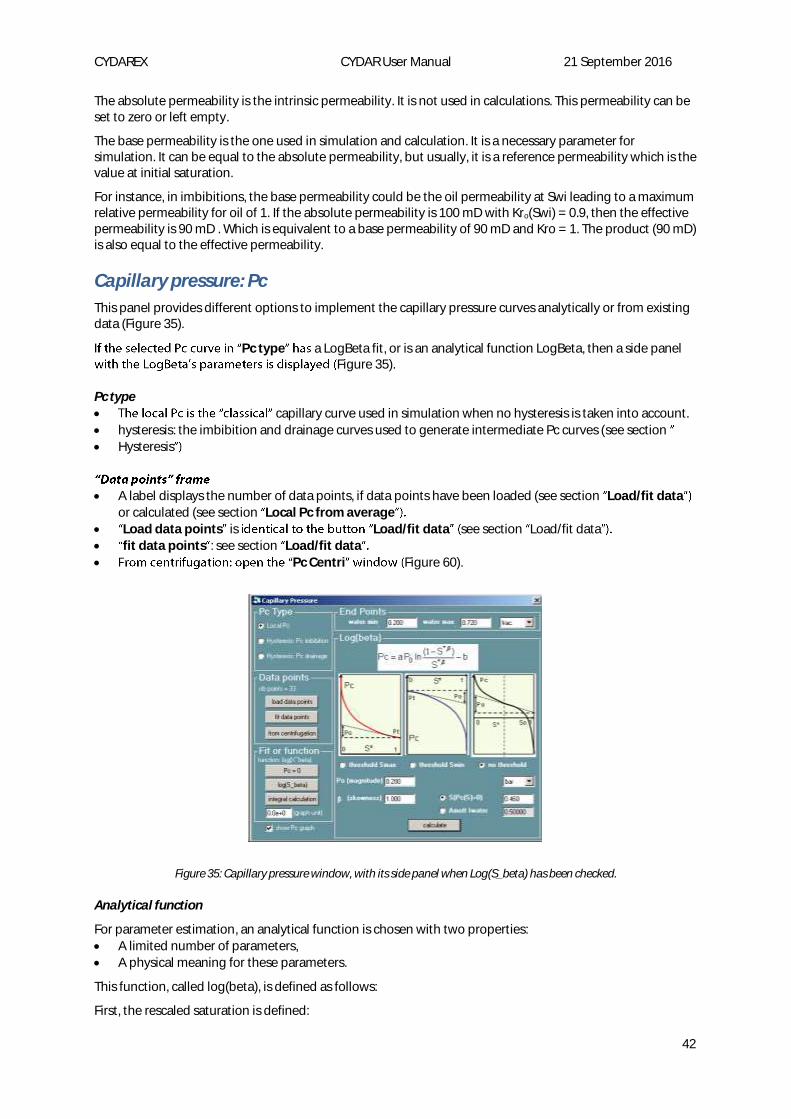
CYDAREX CYDAR User Manual 21 September 2016
42
The absolute permeability is the intrinsic permeability. It is not used in calculations. This permeability can be set to zero or left empty.
The base permeability is the one used in simulation and calculation. It is a necessary parameter for simulation. It can be equal to the absolute permeability, but usually, it is a reference permeability which is the value at initial saturation.
For instance, in imbibitions, the base permeability could be the oil permeability at Swi leading to a maximum relative permeability for oil of 1. If the absolute permeability is 100 mD with Kro(Swi) = 0.9, then the effective permeability is 90 mD . Which is equivalent to a base permeability of 90 mD and Kro = 1. The product (90 mD) is also equal to the effective permeability.
Capillary pressure: Pc
This panel provides different options to implement the capillary pressure curves analytically or from existing data (Figure 35).
Pc type a LogBeta fit, or is an analytical function LogBeta, then a side panel Figure 35).
Pc type
capillary curve used in simulation when no hysteresis is taken into account.
hysteresis: the imbibition and drainage curves used to generate intermediate Pc curves (see section
Hysteresis
A label displays the number of data points, if data points have been loaded (see section Load/fit data
or calculated (see section Local Pc from average
Load data points is Load/fit data see section Load/fit data
fit data points : see section Load/fit data
Pc Centri Figure 60).
Figure 35: Capillary pressure window, with its side panel when Log(S_beta) has been checked.
Analytical function
For parameter estimation, an analytical function is chosen with two properties:
A limited number of parameters,
A physical meaning for these parameters.
This function, called log(beta), is defined as follows:
First, the rescaled saturation is defined:

CYDAREX CYDAR User Manual 21 September 2016
43
𝑆∗ =𝑆−𝑆min
𝑆max−𝑆min.
The general function with no threshold is defined by:
𝑃𝑐 = −𝐴
𝛽𝑃𝑜 [ln
𝑆∗𝛽
1−𝑆∗𝛽 − ln(1−𝑆∗)𝛽
1−(1−𝑆∗)𝛽] + 𝑏 .
𝑃𝑜 and the saturation 𝑆0 are used which correspond to 𝑃𝑐 = 0, related to 𝑏 by:
𝑏 =𝐴
𝛽𝑃𝑜 [ln
𝑆𝑜∗𝛽
1−𝑆𝑜∗𝛽 − ln
(1−𝑆𝑜∗)𝛽
1−(1−𝑆𝑜∗)𝛽] .
The parameter 𝐴 is calculated for continuity with the limit cases with threshold defined below.
Threshold at the maximum value of saturation (𝑆∗ = 1), either in drainage or imbibition:
𝑃𝑐 ≤ 𝑃𝑡 → 𝑆∗ = 1 ; 𝑃𝑐 > 𝑃𝑡 → 𝑃𝑐 = 𝑃𝑜1
𝑆∗.
At minimum of saturation (𝑆∗ = 0):
𝑃𝑐 ≥ 𝑃𝑡 → 𝑆∗ = 0 ; 𝑃𝑐 < 𝑃𝑡 → 𝑃𝑐 = −𝑃𝑜1
(1−𝑆∗).
Figure 36: Examples of Pc curves obtained with the analytical Log(beta) function with 3 options: threshold Smin (Pt=100 mbar); no threshold (Sat=0.45 at Pc=0 ), and threshold Smax (Pt=100 mbar). For the three curves the magnitude is P0=100 mbar.
Amott Index
Instead of fixing the point at which the Pc curve crosses Pc(S) = 0, the Amott index can be entered (Amott, E., "Observations relating to the wettability of porous rock", Trans. AIME 219, pp. 156 162, 1959.).
For an imbibition, the Amott index is defined as Iw = A / (A+B). For a drainage, the Amott index is defined as Io = B / (A + B).
Relative permeabilities: Kr
The relative permeabilities control panel (Figure 37) gives access to several ways for entering Kr curves:
Experimental Data Points: identical to the button .
Corey and Modified Corey: Power law models.
LET: the LET function, as al., SCA, 2005 (see Reference 4).
JBN: analytical calculation with unsteady state experiment.
End Points
Maximum relative permeabilities.
Interval of saturation.
saturation
capil
lary
pre
ssu
re
0 1
0 Sor
A B
Swi
saturation
capil
lary
pre
ssu
re
0 1
0
saturation
capil
lary
pre
ssu
re
0 1
0 Sor
A B
Swi
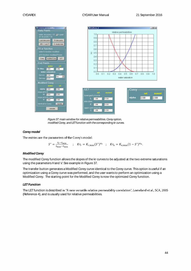
CYDAREX CYDAR User Manual 21 September 2016
44
Corey model
𝑆∗ =𝑆𝑟−𝑆min
𝑆max−𝑆min ; 𝐾𝑟𝑟 = 𝐾𝑟,max(𝑆∗)𝛼𝑟 ; 𝐾𝑟𝑛 = 𝐾𝑛,max(1 − 𝑆∗)𝛼𝑛 .
Modified Corey
The modified Corey function allows the slopes of the kr curves to be adjusted at the two extreme saturations using the parameters H and V. See example in Figure 37.
The transfer button generates a Modified Corey curve identical to the Corey curve. This option is useful if an optimization using a Corey curve was performed, and the user wants to perform an optimization using a Modified Corey. The starting point for the Modified Corey is now the optimized Corey function.
LET Function
The LET function is described (Reference 4), and is usually used for relative permeabilities.
Figure 37: main window for relative permeabilities. Corey option, modified Corey, and LET function with the corresponding kr curves.

CYDAREX CYDAR User Manual 21 September 2016
45
Load/fit data Window
Figure 38: TPF Load/Fit data points window.
Raw data frame: This allows the user to select data to be loaded or edited.
Data corrections frame: The user can perform several data corrections, such as outlet dead volume or offsets. During such corrections, all data points are modified.
Fit/Edit frame: Once a data is selected: Load data points
View/Modify the existing spreadsheet. Remove Edit points edits the data, see the data editing section (Data editing):
interval, removing, adding or moving points, etc.
Fit : fit type specification.
Raw data
Tubing effluents:
Production volumes at the end of tubings. Tubing corrections can be made by entering total tubing volumes in the Experiment windows.
Sample Effluents data:
Volume and flow rate productions at end sample versus time of both fluids.
Gas rate at average pressure is gas production flow rate versus time calculated at the mean value of the two outlet pressures.
Volume balance data:
Net volume balance between inflow and outflow versus time for both fluids.
Saturation data:
Average saturation of the reference fluid versus time. Water is always the reference fluid and gas is always the non-reference fluid.
Tdepending on the boundary condition (Table 3).
The calculation cannot be performed with the gas rate at average pressure.
Useful Tips: If the numerical solver is set to uncompressible, the simulated gas rate at average pressure is simply the gas rate at the outlet pressure. To get the real gas rate at average pressure, the numerical solver must be set on compressible.
Useful Tips: When values exist, the name is displayed in a darker background. The saturation is always the reference fluid saturation: water with oil, or liquid in a gas/liquid system.

CYDAREX CYDAR User Manual 21 September 2016
46
Experiment type Inlet boundary conditions Mandatory data
2 fluids injected: constant flow rates 1 fluid injected: constant flow rate Spontaneous Semi-dynamic (SDM)
2 flow rates (or 0) One of the production data: volume, flow rate or volume balance.
2 fluids injected: flow rate, pressure. 1 fluid injected: constant pressure Gravity Centrifugation Porous plate
flow rate (or 0) - pressure
One of the production data of the injected fluid at constant flow rate: volume, flow rate or volume balance.
Table 3 Necessary data to calculate the average saturation according to the experience type.
Pressures data (end-pieces):
Inlet and outlet pressures in end-pieces and their difference versus time.
he analytical fit of the data is used as simulation input.
Kr and Pc data:
Relative permeabilities and capillary pressure data versus reference fluid saturation.
Hysteresis: the imbibition and drainage curves used to generate intermediate Pc curves (see section
K and Phi data: Porosity and permeability data versus length.
Two types of data can be loaded as composite and profile. The composite type is versus length of blocks. The profile data is versus length.
In the composite case, raw data are used as input in simulation; therefore no editing is possible. The sample length is calculated from the sum of lengths.
In the profile case, common editing is possible. If there is no value at 0 or at the sample length, they are linearly extrapolated. See section Heterogeneities
Profiles data:
Initial saturation versus length can be use as input for simulation (see section
Hysteresis ).
Saturation and pressure profiles versus length. These data cannot be edited; they can be use for optimization.
Pc porous plate:
at the extrapolated saturation value calculated from fit (Multi-Step bi-exponential fit);
See section Porous Plate p. 75 for details.
Pc centri:
Sat(Pc) is the average saturation versus capillary pressure;
Sat(speed) is the average saturation versus rotation speed;
Speed(t) is the rotation speed versus time. It can be used as simulation input instead of block time values.
Capillary pressure is calculated from rotation speed, therefore loading Sat(speed) will automatically calculate Sat(Pc).
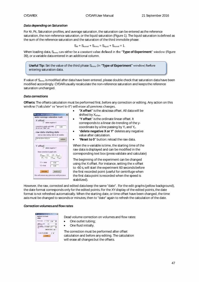
CYDAREX CYDAR User Manual 21 September 2016
47
Data depending on Saturation
For Kr, Pc, Saturation profiles, and average saturation, the saturation can be entered as the reference saturation, the non-reference saturation, or the liquid saturation (Figure 1). The liquid saturation is defined as the sum of the reference saturation and the saturation of the third immobile phase:
Sref + Snonref + Simmo = Sliquid + Snonref = 1.
When loading data, Simmo Type of Experiment Figure 39), or a variable data entered in an additional column.
If value of Simmo is modified after data have been entered, please double check that saturation data have been modified accordingly. CYDAR usually recalculate the non-reference saturation and keeps the reference saturation unchanged.
Data corrections
Offsets: The offsets calculation must be performed first, before any correction or editing. Any action on this
X offset is the abscissa offset. All data will be shifted by Xoffset.
Y offset is the ordinate linear offset. It corresponds to a linear de-trending of the y-coordinate by a line passing by Y1 and Y2.
delete negative X or Y deletes any negative value after calculation.
Reset to 0 button: reload the raw data.
When the x-variable is time, the starting time of the raw data is displayed and can be modified in the corresponding text box (press validate and calculate)
The beginning of the experiment can be changed using the X offset. For instance, setting the x-offset to -60 s, will start the experiment 60 seconds before the first recorded point (useful for centrifuge when the first data point is recorded when the speed is stabilized).
However, the raw, corrected and edited data keep the same "date". For the edit graphs (yellow background), the date format corresponds only for the edited points. For the XY display of the edited points, the date format is not refreshed automatically. When the starting date, or time offset have been changed, the time axis must be changed to seconds or minutes, then to "date" again to refresh the calculation of the date.
Correction volumes and flow rates
Dead volume correction on volumes and flow rates:
One outlet tubing;
One fluid initially.
The correction must be performed after offset calculation and before any editing. The calculation will erase all changes but the offsets.
Useful Tip: Set the value of the third phase Simmo Type of Experimententering saturation data.
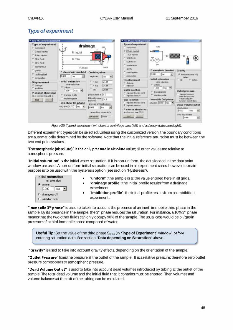
CYDAREX CYDAR User Manual 21 September 2016
48
Type of experiment
Figure 39: Type of experiment windows: a centrifuge case (left) and a steady-state case (right).
Different experiment types can be selected. Unless using the customized version, the boundary conditions are automatically determined by the software. Note that the initial reference saturation must be between the two end points values.
P atmospheric (absolute) value; all other values are relative to atmospheric pressure.
Initial saturation initial water saturation. If it is non-uniform, the data loaded in the data point window are used. A non-uniform initial saturation can be used in all experiment cases, however its main purpose is to be used with the hysteresis option (see section Hysteresis
uniform : the sample is at the value entered here in all grids.
drainage profile : the initial profile results from a drainage experiment.
imbibition profile : the initial profile results from an imbibition experiment.
rd is used to take into account the presence of an inert, immobile third phase in the sample. By its presence in the sample, the 3rd phase reduces the saturation. For instance, a 10% 3rd phase means that the two other fluids can only occupy 90% of the sample. The usual case would be oil/gas in presence of a third immobile phase composed of water.
is used to take into account gravity effects, depending on the orientation of the sample.
fixes the pressure at the outlet of the sample. It is a relative pressure; therefore zero outlet pressure corresponds to atmospheric pressure.
is used to take into account dead volumes introduced by tubing at the outlet of the sample. The total dead volume and the initial fluid that it contains must be entered. Then volumes and volume balances at the exit of the tubing can be calculated.
Useful Tip: Set the value of the third phase Simmo Type of Experimententering saturation data. See section Data depending on Saturation bove.
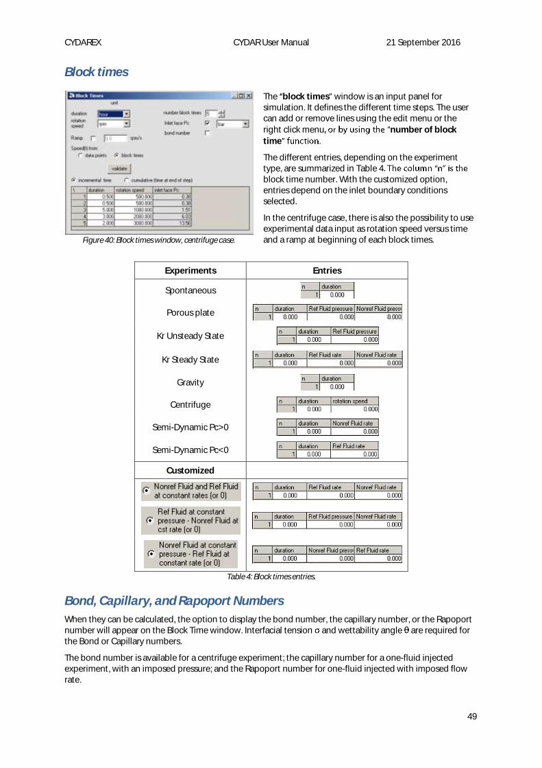
CYDAREX CYDAR User Manual 21 September 2016
49
Block times
Figure 40: Block times window, centrifuge case.
The block times window is an input panel for simulation. It defines the different time steps. The user can add or remove lines using the edit menu or the right click menu number of block
time .
The different entries, depending on the experiment type, are summarized in Table 4block time number. With the customized option, entries depend on the inlet boundary conditions selected.
In the centrifuge case, there is also the possibility to use experimental data input as rotation speed versus time and a ramp at beginning of each block times.
Experiments Entries
Spontaneous
Porous plate
Kr Unsteady State
Kr Steady State
Gravity
Centrifuge
Semi-Dynamic Pc>0
Semi-Dynamic Pc<0
Customized
Table 4: Block times entries.
Bond, Capillary, and Rapoport Numbers
When they can be calculated, the option to display the bond number, the capillary number, or the Rapoport number will appear on the Block Time window. Interfacial tension and wettability angle are required for the Bond or Capillary numbers.
The bond number is available for a centrifuge experiment; the capillary number for a one-fluid injected experiment, with an imposed pressure; and the Rapoport number for one-fluid injected with imposed flow rate.
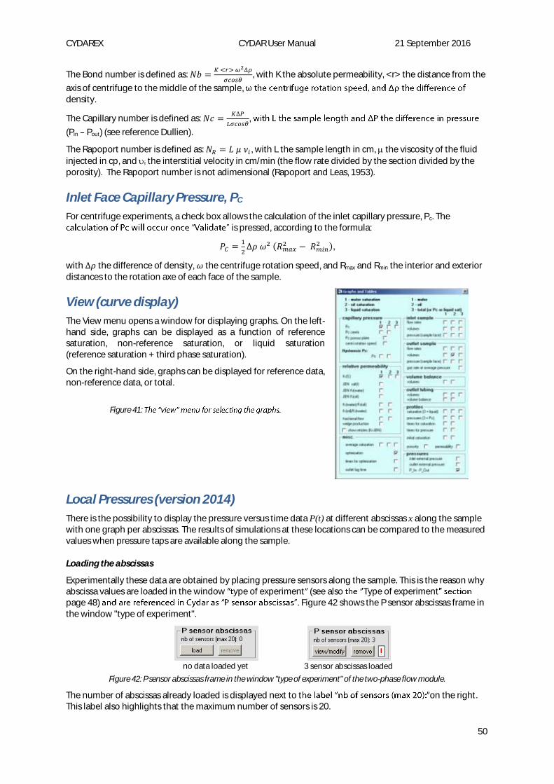
CYDAREX CYDAR User Manual 21 September 2016
50
The Bond number is defined as: 𝑁𝑏 =𝐾 <𝑟> 𝜔2∆𝜌
𝜎𝑐𝑜𝑠𝜃, with K the absolute permeability, <r> the distance from the
axis of centrifuge to the middle of the sample, density.
The Capillary number is defined as: 𝑁𝑐 =𝐾∆𝑃
𝐿𝜎𝑐𝑜𝑠𝜃,
(Pin Pout) (see reference Dullien).
The Rapoport number is defined as: 𝑁𝑅 = 𝐿 𝜇 𝜈𝑖 , with L the sample length in cm, the viscosity of the fluid
injected in cp, and i the interstitial velocity in cm/min (the flow rate divided by the section divided by the porosity). The Rapoport number is not adimensional (Rapoport and Leas, 1953).
Inlet Face Capillary Pressure, PC
For centrifuge experiments, a check box allows the calculation of the inlet capillary pressure, Pc. The is pressed, according to the formula:
𝑃𝐶 =1
2∆𝜌 𝜔2 (𝑅𝑚𝑎𝑥
2 − 𝑅𝑚𝑖𝑛2 ),
with Δ𝜌 the difference of density, 𝜔 the centrifuge rotation speed, and Rmax and Rmin the interior and exterior distances to the rotation axe of each face of the sample.
View (curve display)
The View menu opens a window for displaying graphs. On the left-hand side, graphs can be displayed as a function of reference saturation, non-reference saturation, or liquid saturation (reference saturation + third phase saturation).
On the right-hand side, graphs can be displayed for reference data, non-reference data, or total.
Figure 41:
Local Pressures (version 2014)
There is the possibility to display the pressure versus time data P(t) at different abscissas x along the sample with one graph per abscissas. The results of simulations at these locations can be compared to the measured values when pressure taps are available along the sample.
Loading the abscissas
Experimentally these data are obtained by placing pressure sensors along the sample. This is the reason why abscissa values are loaded in the window ype of experiment (see also Type of experimentpage 48) . Figure 42 shows the P sensor abscissas frame in the window "type of experiment".
no data loaded yet
3 sensor abscissas loaded
Figure 42: P sensor abscissas frame in the window "type of experiment" of the two-phase flow module.
The number of abscissas already loaded is displayed next to t on the right. This label also highlights that the maximum number of sensors is 20.
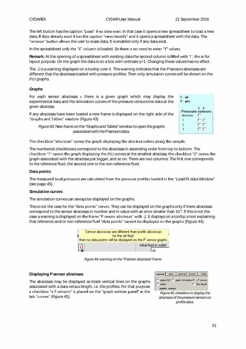
CYDAREX CYDAR User Manual 21 September 2016
51
The left button has the caption . In that case it opens a new spreadsheet to load a new data. it opens a spreadsheet with the data. The
the user to erase data. It is enabled only if any data exist.
In the spreadsheet o is loaded. So
Remark: At the opening of a spreadsheet with existing data the second column is for layout purpose. On the graph the data is on a line with ordinate y=1. Changing these values has no effect.
The is a warning displayed on a tooltip over it. This warning indicates that the P sensors abscissas are different that the abscissas loaded with pressure profiles. Then only simulation curves will be shown on the P(t) graphs.
Graphs
For each sensor abscissas x there is a given graph which may display the experimental data and the simulation curves of the pressure versus time data at the given abscissa.
If any abscissas have been loaded a new frame is displayed on the right side of the Figure 43)
Figure 43: New frame on the "Graphs and Tables" window to open the graphs associated with the P sensors data.
The numbered checkboxes correspond to the abscissas in ascending order from top to bottom. The P(t) curves at the smallest abscissa
graph associated with the abscissa just bigger, and so on. There are two columns. The first one corresponds to the reference fluid, the second one to the non-reference fluid.
Data points
The meas Load/fit data Window(see page 45).
Simulation curves
The simulation curves can always be displayed on the graphs.
This is not the case for the They can be displayed on the graphs only if there abscissas correspond to the sensor abscissas in number and in value with an error smaller than 10-3. If this is not the case a warning is displayed on . It displays on a tooltip a text explaining that reference and/or non-reference (Figure 44).
Figure 44: warning on the "P sensor abscissas" frame.
Displaying P sensor abscissas
The abscissas may be displayed as black vertical lines on the graphs associated with a data versus length, i.e. the profiles. For that purpose
Figure 45).
Figure 45: checkbox to display the
abscissas of the pressure sensors on profile data.

CYDAREX CYDAR User Manual 21 September 2016
52
Interfacial tension and viscosities values per block time (version 2016)
The purpose is to simulate a waterflood (imbibition) followed by injection of a surfactant or a polymer. Low surface tension or high viscosity increases the viscous forces compared to capillary forces and reduce the "capillary end effect". The change of fluid properties at end of simulation allows the quantification of recovery due to this effect.
It is possible to enter different IFT and viscosity values at each block times. It is first enabled in the block times IFT and viscosity units
comboboxes as well three more columns on the left (Figure 46).
Figure 46: Block times window with the IFT and viscosities columns enabled.
Values
By default all the IFT column values are set to zero and the viscosities are set to the values entered in the
The IFT or viscosities change between BT are disabled in simulation if all BT values are equal. Therefore, if all the IFT values are zero, which is the default, the IFT change between block times is disabled in simulation.
The viscosities cannot be set to zero. If a zero is entered the value is set to its default value.
An error occurs if one of the values is zero or negative.
IFT Viscosities
Default values 0
Viscosity entered in the
window.
Disabled If all values are equal If all values are equal
Error if enabled One of the value is zero or negative
One of the value is zero or negative
Enabling the IFT and viscosities change between block times in simulation
-window. This checkbowindow.
If enabled the viscosity used in simulation is the one defined in the block times. Therefore, if the viscosity rent to the first BT value the value in the sample window is
not used for simulation.

CYDAREX CYDAR User Manual 21 September 2016
53
IFT change implementation
The effect of the change of the interfacial tension is implemented only on the capillary pressure not on the relative permeability.
Using the assumption that the Leverett function is constant on the same rock type we can write that the Leverett function of the block time i is equal to the Leverett function of the block times i+1:
𝐽𝑖 = 𝐽𝑖+1
𝑃𝑐𝑖
𝛾𝑖 cos𝜃𝑖
√𝐾
𝜙=
𝑃𝑐𝑖+1
𝛾𝑖+1 cos𝜃𝑖+1
√𝐾
𝜙
Therefore, we have between block time i and block time i+1:
𝑃𝑐𝑖+1= 𝑃𝑐𝑖
𝛾𝑖+1 cos𝜃𝑖+1
𝛾𝑖 cos𝜃𝑖
Remark: the IFT column contains the values 𝛾 cos 𝜃 which have the same dimension than an interfacial tension.
Viscosity change implementation
The
𝑈 =𝐾 𝐾𝑟
𝜇
𝜕𝑃
𝜕𝑥
The change of viscosity intervenes in the mobility factor 𝐾 𝐾𝑟/𝜇. Therefore, to account for the change of the viscosity between two block times we just need to multiply the mobility factor by the viscosity ratio 𝜇𝑖/𝜇𝑖+1.
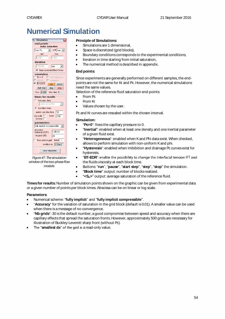
CYDAREX CYDAR User Manual 21 September 2016
54
Numerical Simulation
Figure 47: The simulation
window of the two-phase flow module.
Principle of Simulations:
Simulations are 1 dimensional,
Space is discretized (grid blocks),
Boundary conditions corresponds to the experimental conditions,
Iteration in time starting from initial saturation,
The numerical method is described in appendix.
End points:
Since experiments are generally performed on different samples, the end-points are not the same for Kr and Pc. However, the numerical simulations need the same values. Selection of the reference fluid saturation end-points:
From Pc
From Kr
Values chosen by the user.
Pc and Kr curves are rescaled within the chosen interval.
Simulation:
Pc=0 : fixes the capillary pressure to 0.
Inertial : enabled when at least one density and one inertial parameter of a given fluid exist.
Heterogeneous : enabled when K and Phi data exist. When checked, allows to perform simulation with non-uniform K and phi.
Hysteresis : enabled when imbibition and drainage Pc curves exist for hysteresis.
BT-EORthe fluids viscosity at each block time.
Buttons: run , pause , start step , step , stop the simulation.
Block time output: number of blocks realized.
<Sw> output: average saturation of the reference fluid.
Times for results: Number of simulation points shown on the graphic can be given from experimental data or a given number of points per block times. Abscissa can be on linear or log scale.
Parameters:
Numerical scheme: fully implicit and fully implicit compressible .
Accuracy for the variation of saturation in the grid block (default is 0.01). A smaller value can be used when there is a message of no-convergence.
Nb grids : 30 is the default number, a good compromise between speed and accuracy when there are capillary effects that spread the saturation fronts. However, approximately 500 grids are necessary for illustration of Buckley-Leverett sharp front (without Pc).
smallest dx a read-only value.
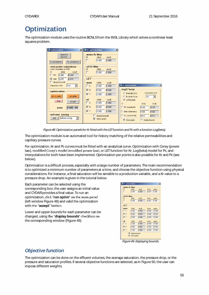
CYDAREX CYDAR User Manual 21 September 2016
55
Optimization The optimization module uses the routine BCNLS from the IMSL Library which solves a nonlinear least squares problem.
Figure 48: Optimization panels for Kr fitted with the LET function and Pc with a function Log(beta).
The optimization module is an automated tool for history matching of the relative permeabilities and capillary pressure curves.
For optimization, Kr and Pc curves must be fitted with an analytical curve. Optimization with Corey (power law), , or LET function for Kr; Log(beta) model for Pc, and interpolations for both have been implemented. Optimization per points is also possible for Kr and Pc (see below).
Optimization is a difficult process, especially with a large number of parameters. The main recommendation is to optimized a minimum number of parameters at a time, and choose the objective function using physical considerations. For instance, a final saturation will be sensible to a production variable, and a Kr value to a pressure drop. An example is given in the tutorial below.
Each parameter can be selected using the corresponding box; the user assigns an initial value and CYDAR provides a final value. To run an
optimization, run optim(left window Figure 48) and valid the optimization with accept
Lower and upper bounds for each parameter can be changed, using display boundsthe corresponding window (Figure 49).
Figure 49: displaying bounds.
Objective function
The optimization can be done on the effluent volumes, the average saturation, the pressure drop, or the pressure and saturation profiles. If several objective functions are selected, as in Figure 50, the user can impose different weights.
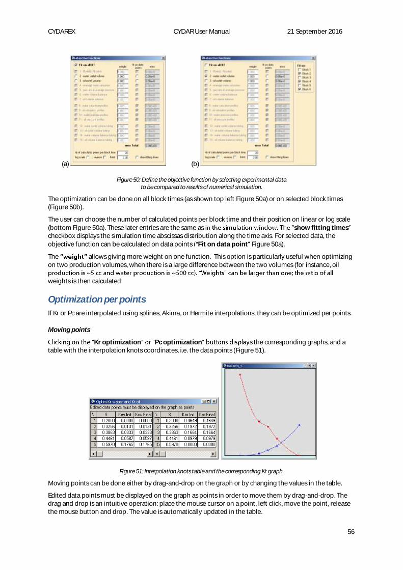
CYDAREX CYDAR User Manual 21 September 2016
56
(a) (b)
Figure 50: Define the objective function by selecting experimental data to be compared to results of numerical simulation.
The optimization can be done on all block times (as shown top left Figure 50a) or on selected block times (Figure 50b).
The user can choose the number of calculated points per block time and their position on linear or log scale (bottom Figure 50a). These later entries are the same as show fitting timescheckbox displays the simulation time abscissas distribution along the time axis. For selected data, the objective function can be calculated on data points Fit on data point Figure 50a).
The allows giving more weight on one function. This option is particularly useful when optimizing on two production volumes, when there is a large difference between the two volumes (for instance, oil
weights is then calculated.
Optimization per points
If Kr or Pc are interpolated using splines, Akima, or Hermite interpolations, they can be optimized per points.
Moving points
Kr optimization Pc optimization s the corresponding graphs, and a table with the interpolation knots coordinates, i.e. the data points (Figure 51).
Figure 51: Interpolation knots table and the corresponding Kr graph.
Moving points can be done either by drag-and-drop on the graph or by changing the values in the table.
Edited data points must be displayed on the graph as points in order to move them by drag-and-drop. The drag and drop is an intuitive operation: place the mouse cursor on a point, left click, move the point, release the mouse button and drop. The value is automatically updated in the table.
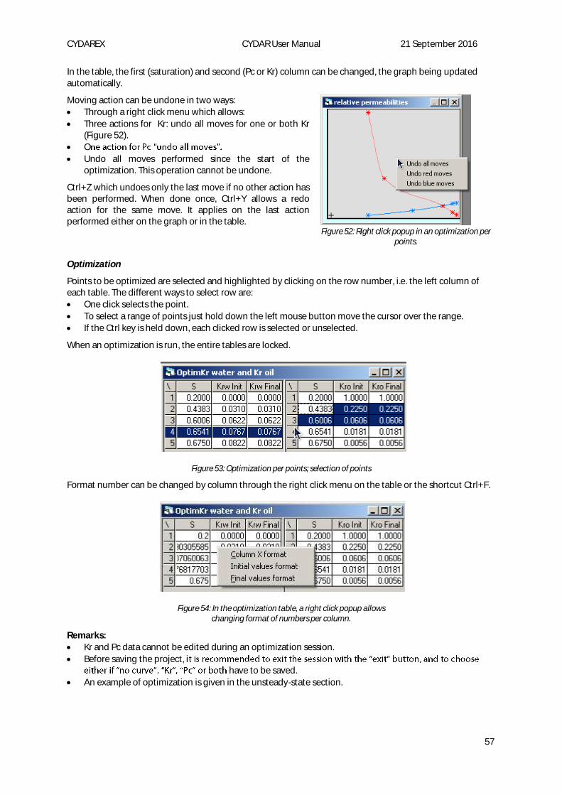
CYDAREX CYDAR User Manual 21 September 2016
57
In the table, the first (saturation) and second (Pc or Kr) column can be changed, the graph being updated automatically.
Moving action can be undone in two ways:
Through a right click menu which allows:
Three actions for Kr: undo all moves for one or both Kr (Figure 52).
O
Undo all moves performed since the start of the optimization. This operation cannot be undone.
Ctrl+Z which undoes only the last move if no other action has been performed. When done once, Ctrl+Y allows a redo action for the same move. It applies on the last action performed either on the graph or in the table.
Figure 52: Right click popup in an optimization per points.
Optimization
Points to be optimized are selected and highlighted by clicking on the row number, i.e. the left column of each table. The different ways to select row are:
One click selects the point.
To select a range of points just hold down the left mouse button move the cursor over the range.
If the Ctrl key is held down, each clicked row is selected or unselected.
When an optimization is run, the entire tables are locked.
Figure 53: Optimization per points; selection of points
Format number can be changed by column through the right click menu on the table or the shortcut Ctrl+F.
Figure 54: In the optimization table, a right click popup allows changing format of numbers per column.
Remarks:
Kr and Pc data cannot be edited during an optimization session.
Before saving the project, ihave to be saved.
An example of optimization is given in the unsteady-state section.

CYDAREX CYDAR User Manual 21 September 2016
58
Unsteady state
Analytical methods (JBN)
For a 1 fluid injected analytical JBN button is enabled in the calculationmain window (Figure 33), and JBN-Jones and Roszelle can be open (Figure 55).
Window JBN-Jones and Roszelle
Injection frame:
Type of displacement: drainage or imbibition
Type of injection: Constant flow rate or constant pressure
Breakthrough time: The breakthrough time must be given because calculations are only valid when the two fluids are produced. Corresponding volume is an output, for verification with the experimental value.
Figure 55: Window for JBN calculation.
The user can specify the number of points and several constrains such as removing negative values.
Jones-Roszelle: Smoothing the intermediate curves (Kr and saturation as a function of time) is equivalent to the Jones and Roszelle method. Using linear The schematic display of the Kr curves allows changing the end-point values if necessary. These curves can be displayed either versus water saturation or oil saturation.
Curve fitting: Data points
points can be fitted either using the JBN window or the general window for data editing.
IMPORTANT: JBN calculation assumes that the capillary pressure is negligible. The standard method to determine the Kr must introduce the measured or estimated Pc, and use optimizations (see the corresponding section).
Multistep one fluid injected
The JBN method is valid only with the unsteady state experiment, with either a constant flow rate or a constant pressure.

CYDAREX CYDAR User Manual 21 September 2016
59
In a first step, saturation and relative permeabilities are calculated as functions of time from the effluent volumes and pressure drop measurements. Then the time is eliminated and Kr are given as a function of saturation.
The different methods called JBN (from Johnson, Bossler and Neuman), Welge, or Jones and Roszelle are based on the same analytical calculation.
If, due to experimental noise, saturation is a non-monotonic function of time, then several different values of Kr can correspond to the same value of saturation (Figure 56). This issue can be avoided by using the Jones and Roszelle method, which smooth the saturation and Kr as a function of time before eliminating the time variable.
Figure 56: Example of Kr determination with noisy data leading to several Kr values.
Tutorial Kr_USS_MW
This is a synthetic case of water/oil imbibition where the experimental data are calculated using a direct numerical simulation; then the parameters are determined and compared to the initial values.
The tutorial contains several files placed in the folder KrUSS:
Tutorial_Kr_USS_MW.xls: Microsoft Excel file with the experimental data, sample, fluids, production, and pressure drop.
Tutorial_Kr_USS_MW_direct.cyd:
Tutorial_Kr_USS_MW.cyd: starting a CYDAR project with the sample and fluids properties, experimental conditions, block times values, experimental data (average saturation and delta pressure). There is no Pc or Kr.
Tutorial_Kr_USS_MW_JBN.cyd: analytical calculation of Kr done from experimental data, Kr fitted with power law (Corey) for optimization, and analytical Pc.
Tutorial_Kr_USS_MW_optim_initial.cyd. This file is the starting point for numerical optimization. For this purpose, the JBN Kr has been fitted with the Corey functions to allow parameter adjustments.
Tutorial_Kr_USS_MW_optim_final.cyd: final results after optimization.
Starting a project
; the default experimental type is set the data:
info sample/fluids
experiment ; displacement set to imbibit ;
Load/fit Data and load data points
At this stage, the project should be equivalent to Tutorial_Kr_USS_MW.cyd. If the numerical simulation button is pressed, an error message is displayed saying that no relative permeabilities are set.
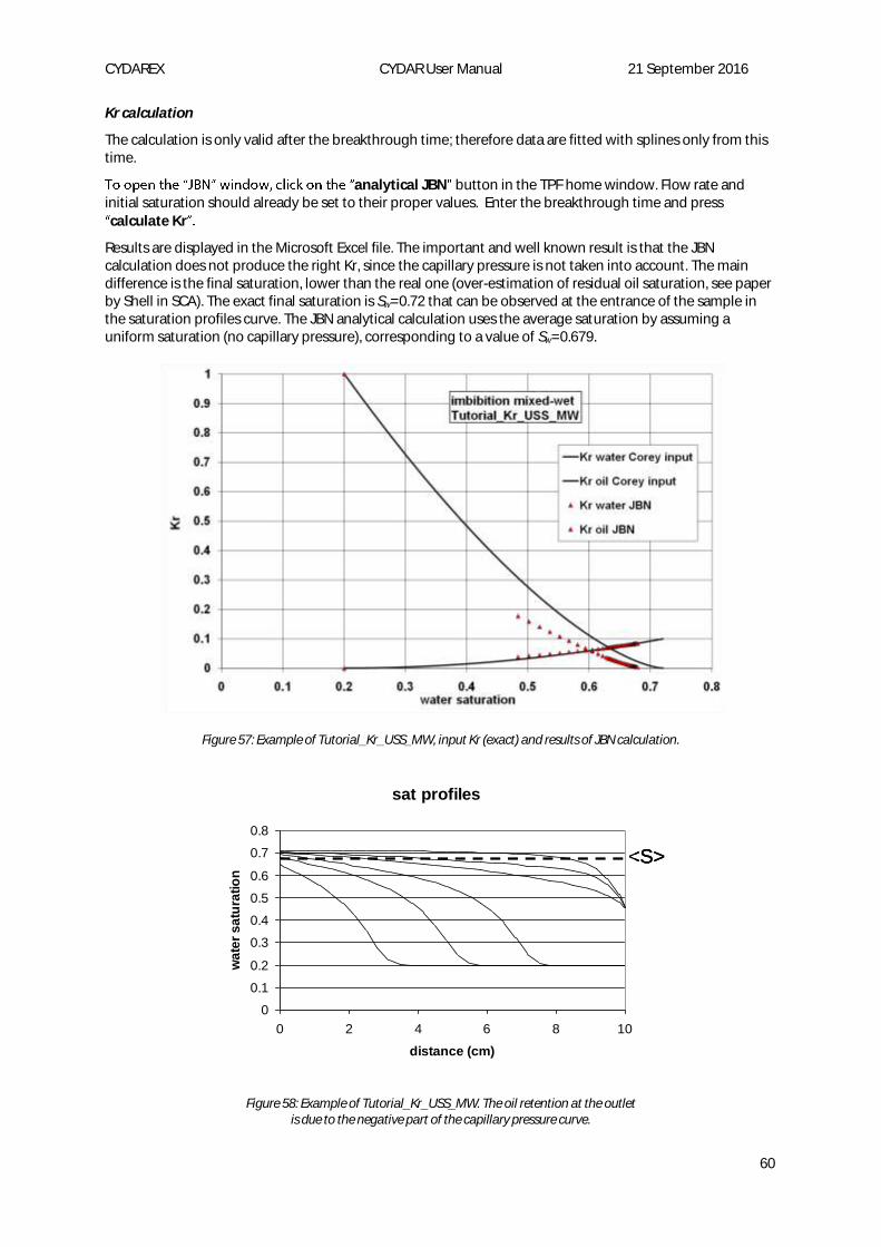
CYDAREX CYDAR User Manual 21 September 2016
60
Kr calculation
The calculation is only valid after the breakthrough time; therefore data are fitted with splines only from this time.
analytical JBN button in the TPF home window. Flow rate and initial saturation should already be set to their proper values. Enter the breakthrough time and press calculate Kr
Results are displayed in the Microsoft Excel file. The important and well known result is that the JBN calculation does not produce the right Kr, since the capillary pressure is not taken into account. The main difference is the final saturation, lower than the real one (over-estimation of residual oil saturation, see paper by Shell in SCA). The exact final saturation is Sw=0.72 that can be observed at the entrance of the sample in the saturation profiles curve. The JBN analytical calculation uses the average saturation by assuming a uniform saturation (no capillary pressure), corresponding to a value of Sw=0.679.
Figure 57: Example of Tutorial_Kr_USS_MW, input Kr (exact) and results of JBN calculation.
Figure 58: Example of Tutorial_Kr_USS_MW. The oil retention at the outlet is due to the negative part of the capillary pressure curve.
sat profiles
0
0.1
0.2
0.3
0.4
0.5
0.6
0.7
0.8
0 2 4 6 8 10
distance (cm)
wa
ter
sa
tura
tio
n
<S>
sat profiles
0
0.1
0.2
0.3
0.4
0.5
0.6
0.7
0.8
0 2 4 6 8 10
distance (cm)
wa
ter
sa
tura
tio
n
<S>
sat profiles
0
0.1
0.2
0.3
0.4
0.5
0.6
0.7
0.8
0 2 4 6 8 10
distance (cm)
wa
ter
sa
tura
tio
n
<S>
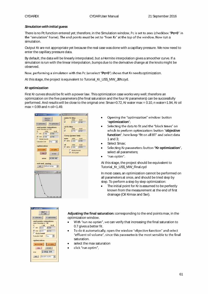
CYDAREX CYDAR User Manual 21 September 2016
61
Simulation with initial guess
There is no Pc function entered yet; therefore, in the Simulation window, Pc=0run a
simulation.
Output Kr are not appropriate yet because the real case was done with a capillary pressure. We now need to enter the capillary pressure data.
By default, the data will be linearly interpolated, but a Hermite interpolation gives a smoother curve. If a simulation is run with the linear interpolation, bumps due to the derivative change at the knots might be observed.
Pc=0 s optimization.
At this stage, the project is equivalent to Tutorial_Kr_USS_MW_JBN.cyd.
Kr optimization
First Kr curves should be fit with a power law. This optimization case works very well; therefore an optimization on the five parameters (the final saturation and the four Kr parameters) can be successfully performed. And results will be close to the original one: Smax=0.72, Kr water max = 0.10, n water=1.94, Kr oil max = 0.99 and n oil=1.49.
optimization
objective function1 and 3;
Select Smax;
Kr optimizationselect all parameters;
At this stage, the project should be equivalent to Tutorial_Kr_USS_MW_Final.cyd
In most cases, an optimization cannot be performed on all parameters at once, and should be tried step by step. To perform a step by step optimization:
The initial point for Kr is assumed to be perfectly known from the measurement at the end of first drainage (Oil Krmax and Swi).
Adjusting the final saturation: corresponding to the end points max, in the optimization window.
e can verify that increasing the final saturation to 0.7 gives a better fit.
saturation.
select the max saturation

CYDAREX CYDAR User Manual 21 September 2016
62
acceptoptimization. To converge, the initial value must be close to the optimized one. Accept this value.
The optimization graph shows the change in the error during the simulation. When a stable value is obtained on this curve, the optimization can be stopped using the stop button. Wait for the complete stop of the process before accepting the value (the mouse index changes from the hour-glass to the arrow). The simulation can also be stopped using the stop button in the simulation window or using the ESC key on the keyboard.
has found a value that minimizes the objective error.
Adjusting water Kr max
We observe that the simulated pressure (DP) in red is higher than the experimental one. At the end of the experiment, oil is no longer produced and water is mainly flowing by itself. Consequently, the final pressure drop is mainly controlled by the relative permeability of water and roughly proportional to the krmax value.
To adjust this parameter automatically, check the fitting box and select delta pressure in the objective run optim Krmax = 0.1.
Adjusting the Kr change the production. We can redo the optimization for the final saturation to have a better fit.
Adjusting both water Kr max, its Corey exponent, and final saturation
Now that the values are close to the optimum, all three parameters can be adjusted together.
Check the three boxes for fit and select both oil volume and pressure difference in the objective function (weight can be kept to unity for each variable). The fit is not so much improved.
Adjusting all parameters
We can optimize all five parameters together. That gives a very good fit with values close to the originals: Smax=0.72, Kr max water = 0.10, n water = 2.01, Kr oil max = 1.00 and n oil = 1.4.
Steady-state
Analytical
The use of this module requires using either the average saturation or the effluent volumes. This method assumes a uniform saturation along the sample, an assumption that is never valid due to the presence of capillary forces. The result must be considered as a first guess for a more accurate method taking into account the capillary pressure (numerical optimization).

CYDAREX CYDAR User Manual 21 September 2016
63
Figure 59: Kr steady-state window and the corresponding Kr result.
Calculation steps:
Selecting the proper units for the flow rates, pressure, and saturation;
Entering the initial saturation. By default this value is the one entered in the experiment window;
Entering the flow rate columns. They are the same as the bloc times columns, unless the user does not want to perform calculation on all bloc times. Bloc times are not necessary.
Pressure diff. and saturation columns are the equilibrium values on each step, or, if equilibrium was not reached on each step, the value at the end of step.
calculate Kr s the calculation.
to see results.
Tutorial
This is a synthetic case of water/oil imbibition where experimental data are calculated using a direct numerical simulation, and parameters are determined and compared to the initial values.
The tutorial contains several files placed in the folder SteadyState:
Tutorial_Kr_SteadyState_OW.xls: Microsoft Excel file with the experimental data, sample, fluids, production, and pressure drop.
Tutorial_Kr_SteadyState_OW_direct.cyd:
Tutorial_Kr_SteadyState_OW.cyd: CYDAR project with sample and fluids properties, experimental conditions, the block times values, and experimental data (average saturation and delta pressure). There are no Pc and Kr yet.
Tutorial_Kr_SteadyState_OW_Kr.cyd: analytical calculation of Kr done from experimental data, Kr fitted with power law (Corey) for optimization, and analytical Pc.
Starting a project
First, sta . This sets the the following data:
info , sample/fluids
experimental conditions (here most of experiment
saturation is 0.2.
Useful Tip: If after calculation, the graph does not show any data, open the graph properties window and select the curves to be displayed.
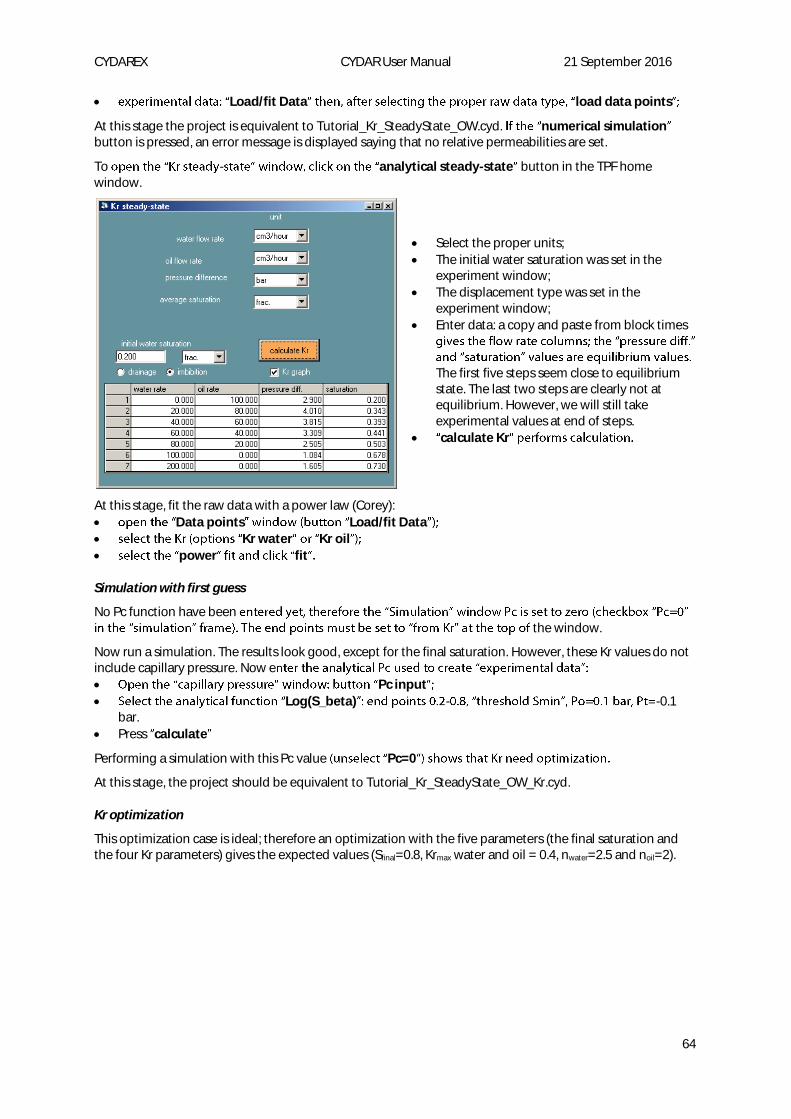
CYDAREX CYDAR User Manual 21 September 2016
64
Load/fit Data load data points
At this stage the project is equivalent to Tutorial_Kr_SteadyState_OW.cyd. numerical simulationbutton is pressed, an error message is displayed saying that no relative permeabilities are set.
To - analytical steady-state button in the TPF home window.
Select the proper units;
The initial water saturation was set in the experiment window;
The displacement type was set in the experiment window;
Enter data: a copy and paste from block times
The first five steps seem close to equilibrium state. The last two steps are clearly not at equilibrium. However, we will still take experimental values at end of steps.
calculate Kr
At this stage, fit the raw data with a power law (Corey):
Data points Load/fit Data
Kr water Kr oil
power fit
Simulation with first guess
No Pc function have been the window.
Now run a simulation. The results look good, except for the final saturation. However, these Kr values do not include capillary pressure. Now e
Pc input
Log(S_beta) - -0.1 bar.
Press calculate
Performing a simulation with this Pc value Pc=0
At this stage, the project should be equivalent to Tutorial_Kr_SteadyState_OW_Kr.cyd.
Kr optimization
This optimization case is ideal; therefore an optimization with the five parameters (the final saturation and the four Kr parameters) gives the expected values (Sfinal=0.8, Krmax water and oil = 0.4, nwater=2.5 and noil=2).

CYDAREX CYDAR User Manual 21 September 2016
65
optimization
block times
objective function fit on all BT t data 1 and 4;
Select S max;
Kr optimizationselect all parameters;
run optim
At this stage, the project is equivalent to Tutorial_Kr_SteadyState_OW_Optim_Final.cyd.
Centrifuge Historically, centrifuge has been used to measure Pc curves in positive drainage and negative imbibition. Now it is also used to determine parts of the relative permeability curves in single or multi-speed experiments using numerical optimization.
Local Pc from average
The main window is accessible either from CYDAR main window bufrom centrifuge can be entered as saturation (not local) versus Pc
or saturation versus speed. In each case, CYDAR automatically provides the second one.
There are three analytical methods to calculate the local Pc curve from the average Pc curve (option choice method Figure 60)):
Hassler-Brunner
Forbes continuousCalculations are performed on the analytical fit of the data and are more accurate.
Forbes + splines
There is one quality control tool:
Pc(<S>) from Pc(S) (see section Tutorial Pc calculation: Comparison CYDAR Forbes SCA ). It allows to check a local Pc curve comparing experimental data and calculated Pc(<S>) curve.
Optimization tool
CYDAR provides an automatic tool to optimize the local Pc curve Pc(S), such as the calculated average curve Pc(<S>) fits better the experimental average data. The Forbes continuous calculation is used as a first guess.
Useful Tip: Most of the time, an optimization must be performed step by step as shown Tutorial Kr_USS_MW .

CYDAREX CYDAR User Manual 21 September 2016
66
Figure 60: Pc centrifuge.
Figure 61: Parameters for the Pc centrifuge calculation
The user can control several parameters (Figure 61).
HB or Forbesthe average saturation (default 1000).
Forbespressure.
splinesdistribution, fit on data points or fit on the smoothed curve (with number of points, default 50).
Tutorial Pc calculation: Comparison CYDAR Forbes SCA
Files:
Tutorial_PcCentri_Drainage_analytical.xls
Tutorial_PcCentri_Drainage_analytical_simulation.cyd
Tutorial_PcCentri_Drainage_Cydar_Optim.cyd
Tutorial_PcCentri_Drainage_Forbes_5_Pts.cyd
In the following section, Pc(S) refers to local capillary pressure curve and Pc(<S>) refers to the capillary pressure versus averaged saturation curve.
Because of the difference in the shape of the capillary pressure curve in imbibition and drainage, the position of the knots for calculation of the splines function usually needs to be adjusted as following:
For a drainage: In the parameter window, the reverse log scale parameter should be unchecked.
For an imbibition: In the parameter window, the reverse log scale parameter should be checked.
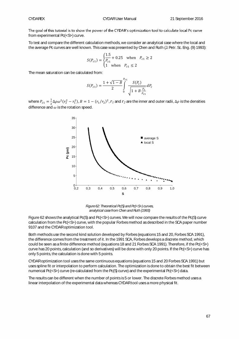
CYDAREX CYDAR User Manual 21 September 2016
67
from experimental Pc(<S>) curve.
To test and compare the different calculation methods, we consider an analytical case where the local and the average Pc curves are well known. This case was presented by Chen and Ruth (J. Petr. Sc. Eng. (9) 1993):
𝑆(𝑃𝑐1) = {
1.5
𝑃𝑐1
+ 0.25 when 𝑃𝑐1 ≥ 2
1 when 𝑃𝑐1 ≤ 2
The mean saturation can be calculated from:
𝑆(𝑃𝑐1) =1 + √1 − 𝐵
2∫
𝑆(𝑃𝑐)
√1 + 𝐵𝑃𝑐
𝑃𝑐1
𝑑𝑃𝑐
𝑃𝑐1
0
where 𝑃𝑐1 =1
2Δ𝜌𝜔2(𝑟2
2 − 𝑟12), 𝐵 = 1 − (𝑟1 𝑟2⁄ )2, r1 and r2 are the inner and outer radii, Δ𝜌 is the densities
difference and 𝜔 is the rotation speed.
Figure 62: Theoretical Pc(S) and Pc(<S>) curves, analytical case from Chen and Ruth (1993)
Figure 62 shows the analytical Pc(S) and Pc(<S>) curves. We will now compare the results of the Pc(S) curve calculation from the Pc(<S>) curve, with the popular Forbes method as described in the SCA paper number 9107 and the CYDAR optimization tool.
Both methods use the second kind solution developed by Forbes (equations 15 and 20, Forbes SCA 1991), the difference comes from the treatment of it. In the 1991 SCA, Forbes develops a discrete method, which could be seen as a finite difference method (equations 18 and 21 Forbes SCA 1991). Therefore, if the Pc(<S>) curve has 20 points, calculation (and so derivatives) will be done with only 20 points. If the Pc(<S>) curve has only 5 points, the calculation is done with 5 points.
CYDAR optimization tool uses the same continuous equations (equations 15 and 20 Forbes SCA 1991) but uses spline fit or interpolation to perform calculation. The optimization is done to obtain the best fit between numerical Pc(<S>) curve (re-calculated from the Pc(S) curve) and the experimental Pc(<S>) data.
The results can be different when the number of points is 5 or lower. The discrete Forbes method uses a linear interpolation of the experimental data whereas CYDAR tool uses a more physical fit.
0,2 0,3 0,4 0,5 0,6 0,7 0,8 0,9 1,00
5
10
15
20
25
30
35
average S
local S
S
Pc (
psi)
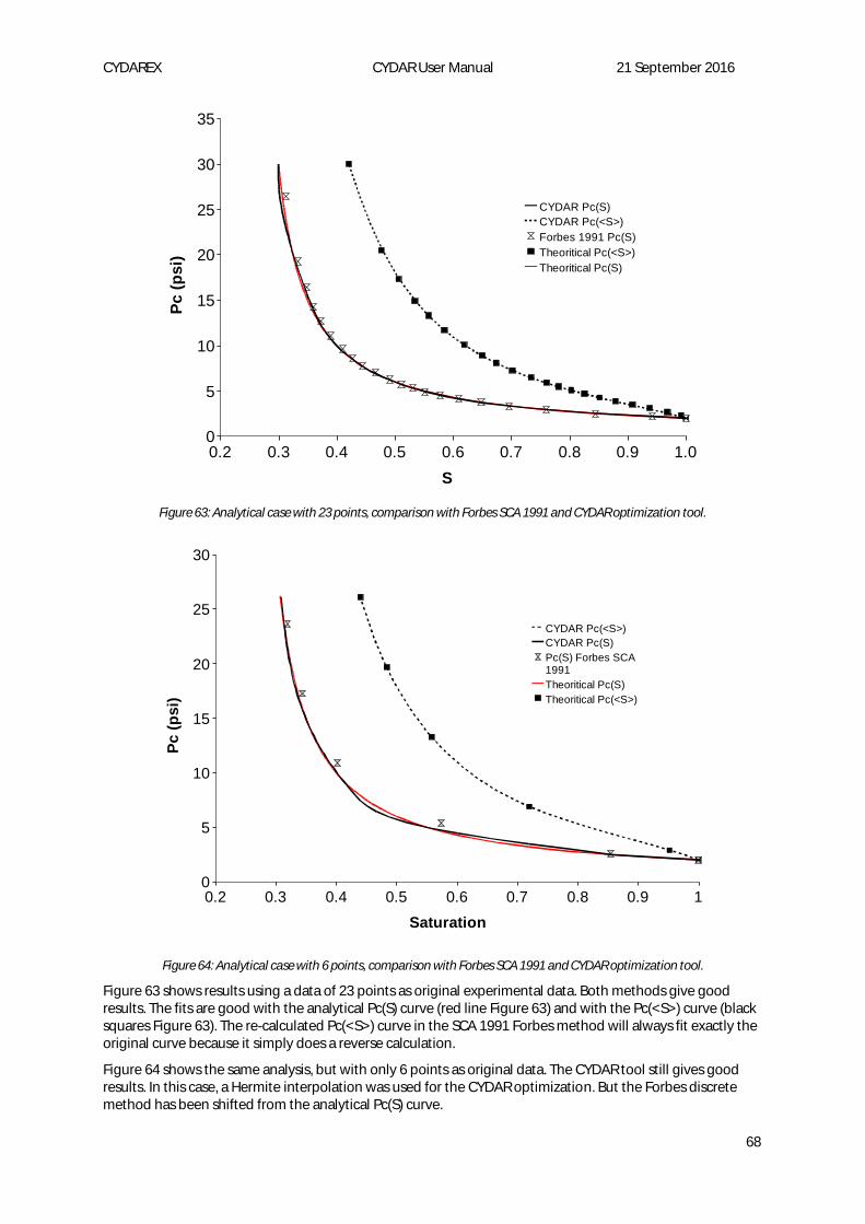
CYDAREX CYDAR User Manual 21 September 2016
68
Figure 63: Analytical case with 23 points, comparison with Forbes SCA 1991 and CYDAR optimization tool.
Figure 64: Analytical case with 6 points, comparison with Forbes SCA 1991 and CYDAR optimization tool.
Figure 63 shows results using a data of 23 points as original experimental data. Both methods give good results. The fits are good with the analytical Pc(S) curve (red line Figure 63) and with the Pc(<S>) curve (black squares Figure 63). The re-calculated Pc(<S>) curve in the SCA 1991 Forbes method will always fit exactly the original curve because it simply does a reverse calculation.
Figure 64 shows the same analysis, but with only 6 points as original data. The CYDAR tool still gives good results. In this case, a Hermite interpolation was used for the CYDAR optimization. But the Forbes discrete method has been shifted from the analytical Pc(S) curve.
0.2 0.3 0.4 0.5 0.6 0.7 0.8 0.9 1.00
5
10
15
20
25
30
35
CYDAR Pc(S)
CYDAR Pc(<S>)
Forbes 1991 Pc(S)
Theoritical Pc(<S>)
Theoritical Pc(S)
S
Pc (
psi)
0.2 0.3 0.4 0.5 0.6 0.7 0.8 0.9 10
5
10
15
20
25
30
CYDAR Pc(<S>)
CYDAR Pc(S)
Pc(S) Forbes SCA 1991
Theoritical Pc(S)
Theoritical Pc(<S>)
Saturation
Pc
(p
si)
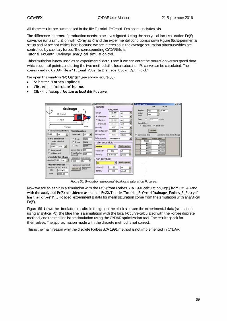
CYDAREX CYDAR User Manual 21 September 2016
69
All these results are summarized in the file Tutorial_PcCentri_Drainage_analytical.xls.
The difference in terms of production needs to be investigated. Using the analytical local saturation Pc(S) curve, we run a simulation with Corey as Kr and the experimental conditions shown Figure 65. Experimental setup and Kr are not critical here because we are interested in the average saturation plateaus which are controlled by capillary forces. The corresponding CYDAR file is Tutorial_PcCentri_Drainage_analytical_simulation.cyd.
This simulation is now used as an experimental data. From it we can enter the saturation versus speed data which counts 6 points, and using the two methods the local saturation Pc curve can be calculated. The
Pc Centri Figure 60):
Forbes + splines
calculate
accept
Figure 65: Simulation using analytical local saturation Pc curve.
Now we are able to run a simulation with the Pc(S) from Forbes SCA 1991 calculation, Pc(S) from CYDAR and
loaded; experimental data for mean saturation come from the simulation with analytical Pc(S).
Figure 66 shows the simulation results. In the graph the black stars are the experimental data (simulation using analytical Pc), the blue line is a simulation with the local Pc curve calculated with the Forbes discrete method, and the red line is the simulation using the CYDAR optimization tool. The results speak for themselves. The approximation made with the discrete method is not correct.
This is the main reason why the discrete Forbes SCA 1991 method is not implemented in CYDAR.
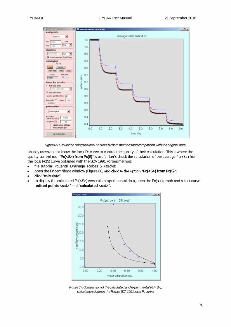
CYDAREX CYDAR User Manual 21 September 2016
70
Figure 66: Simulation using the local Pc curve by both methods and comparison with the original data.
Usually users do not know the local Pc curve to control the quality of their calculation. This is where the Pc(<S>) from Pc(S)
the local Pc(S) curve obtained with the SCA 1991 Forbes method:
file Tutorial_PcCentri_Drainage_Forbes_5_Pts.cyd;
open the Pc centrifuge window (Figure 60 Pc(<S>) from Pc(S)
calculate
to display the calculated Pc(<S>) versus the experimental data, open the Pc(sat) graph and select curve
edited points <sat> calculated <sat>
Figure 67: Comparison of the calculated and experimental Pc(<S>), calculation done on the Forbes SCA 1991 local Pc curve.
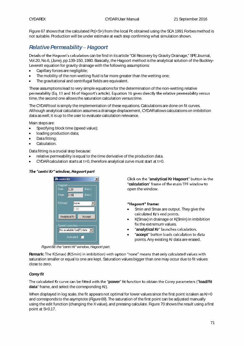
CYDAREX CYDAR User Manual 21 September 2016
71
Figure 67 shows that the calculated Pc(<S>) from the local Pc obtained using the SCA 1991 Forbes method is not suitable. Production will be under estimate at each step confirming what simulation shown.
Relative Permeability Hagoort
can be find in its article "Oil Recovery by Gravity Drainage," SPE Journal, Vol.20, No.6, (June), pp.139-150, 1980. Basically, the Hagoort method is the analytical solution of the Buckley-Leverett equation for gravity drainage with the following assumptions:
Capillary forces are negligible;
The mobility of the non-wetting fluid is far more greater than the wetting one;
The gravitational and centrifugal fields are equivalent.
These assumptions lead to very simple equations for the determination of the non-wetting relative
time, the second one allows the saturation calculation versus time.
The CYDAR tool is simply the implementation of these equations. Calculations are done on fit curves. Although analytical calculation assumes a drainage displacement, CYDAR allows calculations on imbibition data as well; it is up to the user to evaluate calculation relevance.
Main steps are:
Specifying block time (speed value);
loading production data;
Data fitting;
Calculation.
Data fitting is a crucial step because:
relative permeability is equal to the time derivative of the production data.
CYDAR calculation starts at t=0, therefore analytical curve must start at t=0.
Figure 68: the "centri Kr" window, Hagoort part.
analytical Kr Hagoortcalculation
open the window.
Smin and Smax are output. They give the
K(Smax) in drainage or K(Smin) in imbibition fix the extremum values.
analytical Kr
acceptpoints. Any existing Kr data are erased.
Remark: saturation smaller or equal to one are kept. Saturation values bigger than one may occur due to fit values close to zero.
Corey fit
power load/fit data frame, and select the corresponding Kr).
When displayed in log scale, the fit appears not optimal for lower values since the first point is taken as Kr=0 and corresponds to the asymptote (Figure 69). The saturation of the first point can be adjusted manually using the edit function (changing the X value), and pressing calculate. Figure 70 shows the result using a first point at S=0.17.
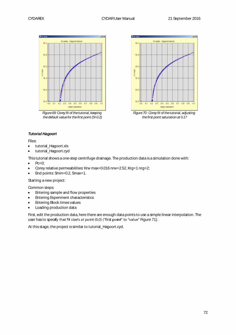
CYDAREX CYDAR User Manual 21 September 2016
72
Figure 69: Corey fit of the tutorial, keeping the default value for the first point (S=0.2)
Figure 70 : Corey fit of the tutorial, adjusting
the first point saturation at 0.17
Tutorial Hagoort
Files:
tutorial_Hagoort.xls
tutorial_Hagoort.cyd
This tutorial shows a one-step centrifuge drainage. The production data is a simulation done with:
Pc=0;
Corey relative permeabilities: Krw max=0.016 nrw=2.52, Krg=1 nrg=2;
End points: Smin=0.2, Smax=1.
Starting a new project:
Common steps:
Entering sample and flow properties
Entering Experiment characteristics
Entering Block times values
Loading production data
First, edit the production data, here there are enough data points to use a simple linear interpolation. The user has to spec first Figure 71).
At this stage, the project is similar to tutorial_Hagoort.cyd.
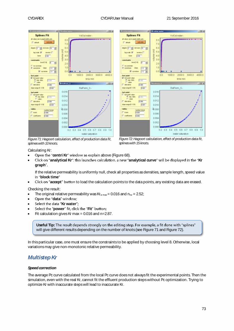
CYDAREX CYDAR User Manual 21 September 2016
73
Figure 71: Hagoort calculation, effect of production data fit, splines with 10 knots.
Figure 72: Hagoort calculation, effect of production data fit, splines with 15 knots.
Calculating Kr:
centri Kr above (Figure 68).
analytical Kr : analytical curve Kr graph
If the relative permeability is uniformly null, check all properties as densities, sample length, speed value block time
accept to load the calculation points to the data points, any existing data are erased.
Checking the result:
The original relative permeability was Krw max = 0.016 and nrw = 2.52;
data
Kr water
power Fit
Fit calculation gives Kr max = 0.016 and n=2.87.
In this particular case, one must ensure the constraints to be applied by choosing level 8. Otherwise, local variations may give non-monotonic relative permeability.
Multistep Kr
Speed correction
The average Pc curve calculated from the local Pc curve does not always fit the experimental points. Then the simulation, even with the real Kr, cannot fit the effluent production steps without Pc optimization. Trying to optimize Kr with inaccurate steps will lead to inaccurate Kr.
Useful Tip: will give different results depending on the number of knots (see Figure 71 and Figure 72).

CYDAREX CYDAR User Manual 21 September 2016
74
In CYDAR, the user has the possibility to correct speed values of block times in order to shift experimental points of the average Pc on the calculated curve.. This is an indirect method to correct for experimental uncertainties on speed values.
The principle is as follow: pressure values of the experimental data are shifted to fit the calculated point at the same saturation. Then the corrected values of speed are calculated from the corrected experimental average Pc curve.
Figure 73 shows an example of experimental average Pc curve shifted to fit the calculated curve. Experimental data points are red stars and the calculated curve is the black line.
Figure 73: speed correction to fit calculated Pc(<S>).
To activate speed correction:
perform Local Pc calculation (see § Local Pc from average)
open the Kr centri window (Figure 68);
choose which calculated average Pc curve to fit;
check the Activated
sat(Pc) sat(speed)identical.
Pc(sat) centri Figure 73 right) are updated. The "Edit Points" graph sat(Pc) sat(speed)will also display the corrected edit points.
To go back to non corrected sat(Pc) sat(speed)data.
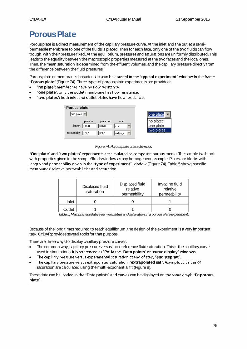
CYDAREX CYDAR User Manual 21 September 2016
75
Porous Plate Porous plate is a direct measurement of the capillary pressure curve. At the inlet and the outlet a semi-permeable membrane to one of the fluids is placed. Then for each face, only one of the two fluids can flow trough, with their pressure fixed. At the equilibrium, pressures and saturations are uniformly distributed. This leads to the equality between the macroscopic properties measured at the two faces and the local ones. Then, the mean saturation is determined from the effluent volumes, and the capillary pressure directly from the difference between the fluid pressures.
Porous plate or membrane characteristics can type of experimentPorous plate Figure 74). Three types of porous plate experiments are provided:
no plate
one plate
two plates
Figure 74: Porous plate characteristics.
One plate two plates rous media. The sample is a block with properties given in the sample/fluids window as any homogeneous sample. Plates are blocks with
type of experiment Figure 74). Table 5 shows specific
Displaced fluid
saturation
Displaced fluid relative
permeability
Invading fluid relative
permeability
Inlet 0 0 1
Outlet 1 1 0 Table 5: Membranes relative permeabilities and saturation in a porous plate experiment.
Because of the long times required to reach equilibrium, the design of the experiment is a very important task. CYDAR provides several tools for that purpose.
There are three ways to display capillary pressure curves:
The common way, capillary pressure versus local reference fluid saturation. This is the capillary curve used in simulations Pc Data points curve display
end step sat
extrapolated sat of saturation are calculated using the multi-exponential fit (Figure 8).
These data can Data points can be displayed on Pc porous plate

CYDAREX CYDAR User Manual 21 September 2016
76
Heterogeneities
Heterogeneity data type
There are three types of heterogeneity in CYDAR. Fluids and sample
Homogeneous
The sample has constant porosity and permeability. The user gives the length, the porosity, and the permeability values.
Composite
The sample is a succession of homogeneous blocks with given length, permeability and porosity.
Figure 75: schematic composite sample.
First, the user loads data:
data points
Data are porosity and permeability values versus lengths of the blocks.
Raw data are used as input in the simulation; any editing is useless and not possible. Permeability and porosity must have the same number of data points and the same length.
Next the heterogeneity type is selected in the Sample and fluids window (p. 41) lengthpermeability, porosity
the harmonic mean for the permeability, and the arithmetic mean for the porosity.
Composite block lengths can Block
length Figure 76).
(K1,Φ
1) (K
2,Φ
2) (K
3,Φ3)
l1
l2
l3
K, Φ
x
(K1,Φ
1) (K
2,Φ
2) (K
3,Φ3)
l1
l2
l3
(K1,Φ
1) (K
2,Φ
2) (K
3,Φ3)(K
1,Φ
1) (K
2,Φ
2) (K
3,Φ3)
l1
l2
l3
K, Φ
x
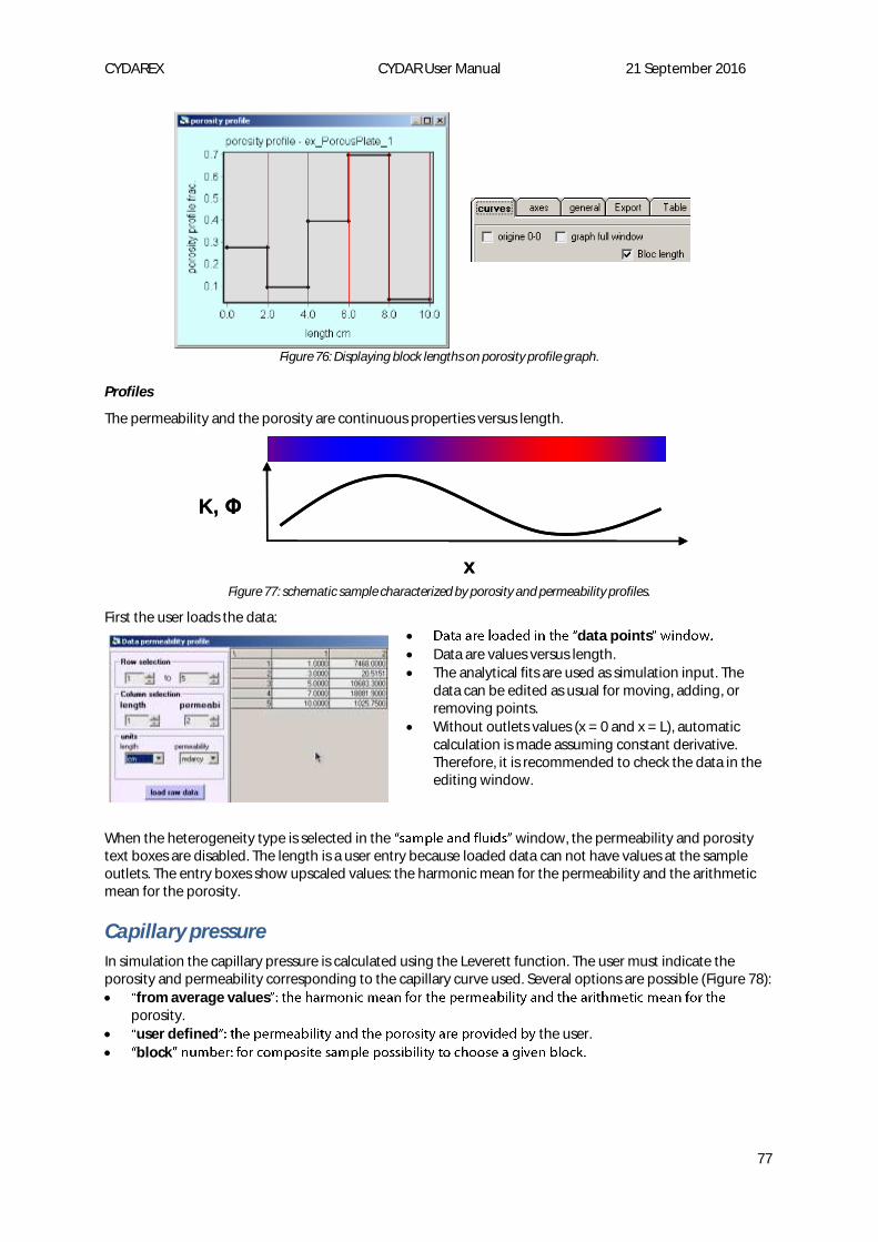
CYDAREX CYDAR User Manual 21 September 2016
77
Figure 76: Displaying block lengths on porosity profile graph.
Profiles
The permeability and the porosity are continuous properties versus length.
Figure 77: schematic sample characterized by porosity and permeability profiles.
First the user loads the data:
data points
Data are values versus length.
The analytical fits are used as simulation input. The data can be edited as usual for moving, adding, or removing points.
Without outlets values (x = 0 and x = L), automatic calculation is made assuming constant derivative. Therefore, it is recommended to check the data in the editing window.
When the heterogeneity type is selected in the window, the permeability and porosity text boxes are disabled. The length is a user entry because loaded data can not have values at the sample outlets. The entry boxes show upscaled values: the harmonic mean for the permeability and the arithmetic mean for the porosity.
Capillary pressure
In simulation the capillary pressure is calculated using the Leverett function. The user must indicate the porosity and permeability corresponding to the capillary curve used. Several options are possible (Figure 78):
from average valuesporosity.
user defined the user.
block
K, Φ
x
K, Φ
x
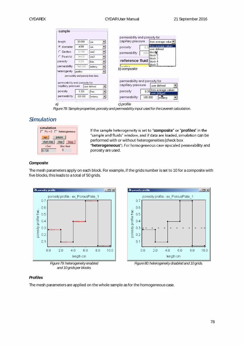
CYDAREX CYDAR User Manual 21 September 2016
78
a)
b) composite
c) profile
Figure 78: Sample properties: porosity and permeability input used for the Leverett calculation.
Simulation
composite profilescan be
performed with or without heterogeneities (check box heterogeneous nd
porosity are used.
Composite
The mesh parameters apply on each block. For example, if the grids number is set to 10 for a composite with five blocks, this leads to a total of 50 grids.
Figure 79: heterogeneity enabled
and 10 grids per blocks.
Figure 80: heterogeneity disabled and 10 grids.
Profiles
The mesh parameters are applied on the whole sample as for the homogeneous case.
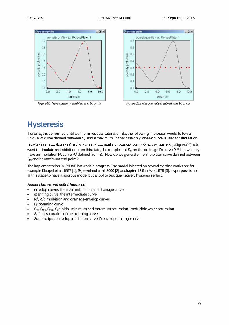
CYDAREX CYDAR User Manual 21 September 2016
79
Figure 81: heterogeneity enabled and 10 grids.
Figure 82: heterogeneity disabled and 10 grids.
Hysteresis If drainage is performed until a uniform residual saturation Swi, the following imbibition would follow a unique Pc curve defined between Swi and a maximum. In that case only, one Pc curve is used for simulation.
ini (Figure 83). We want to simulate an imbibition from this state, the sample is at Sini on the drainage Pc curve PcD, but we only have an imbibition Pc curve PcI defined from Swi. How do we generate the imbibition curve defined between Sini and its maximum end point?
The implementation in CYDAR is a work in progress. The model is based on several existing works see for example Kleppel et al. 1997 [1], Skjaeveland et al. 2000 [2] or chapter 12.6 in Aziz 1979 [3]. Its purpose is not at this stage to have a rigorous model but a tool to test qualitatively hysteresis effect.
Nomenclature and definitions used
envelop curves: the main imbibition and drainage curves
scanning curve: the intermediate curve
PcI, Pc
D: imbibition and drainage envelop curves.
Pc: scanning curve
Sini, Smin, Smax, Swi: initial, minimum and maximum saturation, irreducible water saturation
Sf: final saturation of the scanning curve
Superscripts: I envelop imbibition curve, D envelop drainage curve
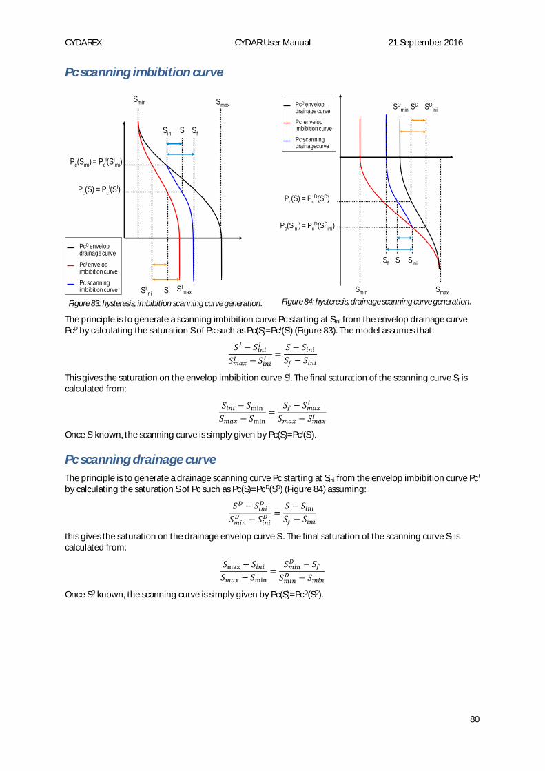
CYDAREX CYDAR User Manual 21 September 2016
80
Pc scanning imbibition curve
Figure 83: hysteresis, imbibition scanning curve generation.
Figure 84: hysteresis, drainage scanning curve generation.
The principle is to generate a scanning imbibition curve Pc starting at Sini from the envelop drainage curve PcD by calculating the saturation S of Pc such as Pc(S)=PcI(SI) (Figure 83). The model assumes that:
𝑆𝐼 − 𝑆𝑖𝑛𝑖𝐼
𝑆𝑚𝑎𝑥𝐼 − 𝑆𝑖𝑛𝑖
𝐼 =𝑆 − 𝑆𝑖𝑛𝑖
𝑆𝑓 − 𝑆𝑖𝑛𝑖
This gives the saturation on the envelop imbibition curve SI. The final saturation of the scanning curve Sf is calculated from:
𝑆𝑖𝑛𝑖 − 𝑆min
𝑆𝑚𝑎𝑥 − 𝑆min
=𝑆𝑓 − 𝑆𝑚𝑎𝑥
𝐼
𝑆𝑚𝑎𝑥 − 𝑆𝑚𝑎𝑥𝐼
Once SI known, the scanning curve is simply given by Pc(S)=PcI(SI).
Pc scanning drainage curve
The principle is to generate a drainage scanning curve Pc starting at Sini from the envelop imbibition curve PcI by calculating the saturation S of Pc such as Pc(S)=PcD(SD) (Figure 84) assuming:
𝑆𝐷 − 𝑆𝑖𝑛𝑖𝐷
𝑆𝑚𝑖𝑛𝐷 − 𝑆𝑖𝑛𝑖
𝐷 =𝑆 − 𝑆𝑖𝑛𝑖
𝑆𝑓 − 𝑆𝑖𝑛𝑖
this gives the saturation on the drainage envelop curve SI. The final saturation of the scanning curve Sf is calculated from:
𝑆max − 𝑆𝑖𝑛𝑖
𝑆𝑚𝑎𝑥 − 𝑆min
=𝑆𝑚𝑖𝑛
𝐷 − 𝑆𝑓
𝑆𝑚𝑖𝑛𝐷 − 𝑆𝑚𝑖𝑛
Once SD known, the scanning curve is simply given by Pc(S)=PcD(SD).
Smin
Pc(Sini) = PcI(SI
ini)
Pc(S) = PcI(SI)
SImax
Sf
SIini
Sini
SI
S
PcD envelopdrainage curve
PcI envelopimbibition curve
Pc scanning imbibition curve
Smax
Pc(Sini) = PcD(SD
ini)
Pc(S) = PcD(SD)
SDmin
Sf
SDini
Sini
SD
S
Smin Smax
PcD envelop drainage curve
PcI envelop imbibition curve
Pc scanning drainagecurve

CYDAREX CYDAR User Manual 21 September 2016
81
Loop
A hysteresis loop is simply a succession of imbibition-drainage, repeated several times. The implementation chosen here is not the popular model. The reason is
progress.
Commonly the second scanning curve in a loop (light blue curve (Figure 85) meets the envelop curve at the origin of the first scanning curve (dark blue curve starting from black curve (Figure 85). For the moment in CYDAR the second scanning curve has the same final saturation calculation that if it is the first scanning curve.
Figure 85 Hysteresis loop
Relative permeabilities
There is no specific treatment for the relative permeability curve unless the change of the local end points depending on the final saturation calculated for the Pc scanning curve.
Non-uniform initial saturation profile
In CYDAR, a non-uniform initial saturation profile can be used. The curve (saturation vs length) is loaded, edited, and fitted as usual (see § Load/fit data).
Type of experimentprocess the origin of the profile (drainage or imbibition experiment) must be known as seen above.
Inertial correction (version 2014) The inertial correction is Permeability Module Inertial correctionpage 35. In the two-phase flow module a local form of the Forchheimer equation is implemented for each fluid:
(𝐹 −𝑑𝑃
𝑑𝑥) =
𝜇
𝐾 𝐾𝑟
𝑈 + 𝛽𝜌𝑈2
with β the inertial coefficient which has the dimension of the inverse of a length, F is the body force equal to 𝜌𝑔 for gravity or 𝜌𝜔2𝑟 in centrifuge.
The inertial coefficients of both fluids are entered in the "fluid and sample properties window (Figure 34). By (Figure
86).
Figure 86: The inertial coefficient entries in the two-phase flow module.
Pc(Sini) = PcD(SD
ini)
Pc(S) = PcD(SD)
SDiniSmin=SD
min
Sini
SD
S
PcD envelop drainage curve
PcI envelop imbibition curve
1st Pc scanning imbibition curve
Pc scanning drainage curve
CYDAREX CYDAR User Manual 21 September 2016
82
The inertial coefficient can be entered as β or in its dimensionless form 𝐵 = 𝛽𝜙√𝐾𝑑 (see page 35). According
to the Forchheimer equation, there is inertial correction only if the fluid density and β are not equal to zero. Therefore if one fluid has a nonzero β but its density is zero, a warning is displayed next to the option button β, on the right.
The inertial correction is active in a simulation on the simulation window (Figure 47). This box is enabled if at least one fluid has nonzero values for its β and density. For example if β and the density are nonzero values for the non-reference fluid, the correction will be active in the simulation only for the non-reference fluid. If both fluids have both parameters not equal to zero then the correction will apply on the two fluids.
Electrical (version 2016)
Purpose
This module based on electrical measurements on local electrodes along the sample has two applications
Determine the local saturation, assuming that the resistivity index is known
Determine the resistivity index using the local saturation obtained by the numerical saturation and the measured effluent production
The two methods can be combined into an optimization loop
Principles
The water saturation may be estimated by the measurement of the resistivity index RI using empirical laws.
The resistivity index is the ratio between the resistivity at a given saturation RS and the resistivity of the fully saturated sample R0
𝑅𝐼(𝑆) =𝑅𝑆
𝑅0
Three models are implemented to calculate the water saturation from measurements:
𝑅𝐼 = 𝑆𝑤−𝑛1
"bending down" and "bending up" laws from Fleury16:
𝑅𝐼 = 𝑆𝑤−𝑛1
1 + 𝐶
1 + 𝐶𝑆𝑤−𝑛2
𝑅𝐼 = 𝑆𝑤−𝑛1
1 + 𝐶𝑆𝑤−𝑛2
1 + 𝐶
C=
Experimental setup possibilities
The measurements are either voltage or resistance at different abscissa along the sample.
If the measures are resistances then the saturation at the electrodes location is calculated directly from the empirical law.
If the measures are voltages then the resistivity is calculated from the tension difference between two electrodes and the current.

CYDAREX CYDAR User Manual 21 September 2016
83
Rload at the inlet
Figure 87: Rload at the inlet
The current is given by
𝐼 =𝑉𝑖𝑛
𝑅𝑙𝑜𝑎𝑑
Rload at the outlet
Figure 88: Rload at the outlet
The current is given by
𝐼 =𝑉𝑜𝑢𝑡 − 𝑉𝑝𝑜𝑤𝑒𝑟
𝑅𝑙𝑜𝑎𝑑
Resistances calculation
The resistances are given by
𝑅1 =𝑉1 − 𝑉𝑖𝑛
𝐼
𝑅𝑖 =𝑉𝑖 − 𝑉𝑖−1
𝐼
𝑅𝑛+1 =𝑉𝑜𝑢𝑡 − 𝑉𝑛
𝐼
The resistivity index along the sample are then calculated using the resistivity value when the sample is fully saturated
𝑅𝐼𝑖 =𝑅𝑖
𝑅0𝑖
Contact resistances
The two extreme resistances contain contact resistance. They may be corrected by using R2 instead of R1 and/or Rn instead of Rn+1.

CYDAREX CYDAR User Manual 21 September 2016
84
Saturation calculation
Local saturations at the abscissa are calculated using one of the three empirical laws from the local resistivity indexes, for instance in the Archies' law case:
𝑆𝑤𝑖= 𝑅𝐼𝑖
−1
𝑛1
The average saturation is calculated by:
< 𝑆𝑤 >=∑𝑑𝑥𝑖 Φ𝑖 𝐴 𝑆𝑖
𝑉𝑝
the dxi are the distances between electrodes if the measures are voltage, around each electrode if the measures are resistances. i is the porosity at the middle of dxi. A is the section and Vp is the total pore volume.
CYDAR module
The sample characteristic, the abscissa, the profiles and the saturated profile are compulsory. If the profiles are voltages, they must contain Vin and Vout.
Vin and Vout are not counted in the data with the electrode abscissa.
Figure 89 and the data versus s.
Electrical method: setup window
Entries of the window are fairly obvious, see below for some explanation.
Figure 89: the "Electrical window" is the window with setup parameters
The experimental data are resistances
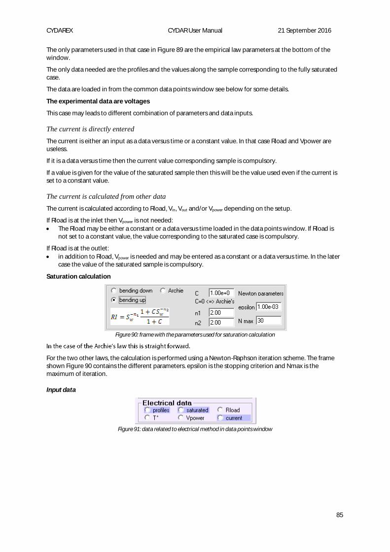
CYDAREX CYDAR User Manual 21 September 2016
85
The only parameters used in that case in Figure 89 are the empirical law parameters at the bottom of the window.
The only data needed are the profiles and the values along the sample corresponding to the fully saturated case.
The data are loaded in from the common data points window see below for some details.
The experimental data are voltages
This case may leads to different combination of parameters and data inputs.
The current is directly entered
The current is either an input as a data versus time or a constant value. In that case Rload and Vpower are useless.
If it is a data versus time then the current value corresponding sample is compulsory.
If a value is given for the value of the saturated sample then this will be the value used even if the current is set to a constant value.
The current is calculated from other data
The current is calculated according to Rload, Vin, Vout and/or Vpower depending on the setup.
If Rload is at the inlet then Vpower is not needed:
The Rload may be either a constant or a data versus time loaded in the data points window. If Rload is not set to a constant value, the value corresponding to the saturated case is compulsory.
If Rload is at the outlet:
in addition to Rload, Vpower is needed and may be entered as a constant or a data versus time. In the later case the value of the saturated sample is compulsory.
Saturation calculation
Figure 90: frame with the parameters used for saturation calculation
For the two other laws, the calculation is performed using a Newton-Raphson iteration scheme. The frame shown Figure 90 contains the different parameters. epsilon is the stopping criterion and Nmax is the maximum of iteration.
Input data
Figure 91: data related to electrical method in data points window
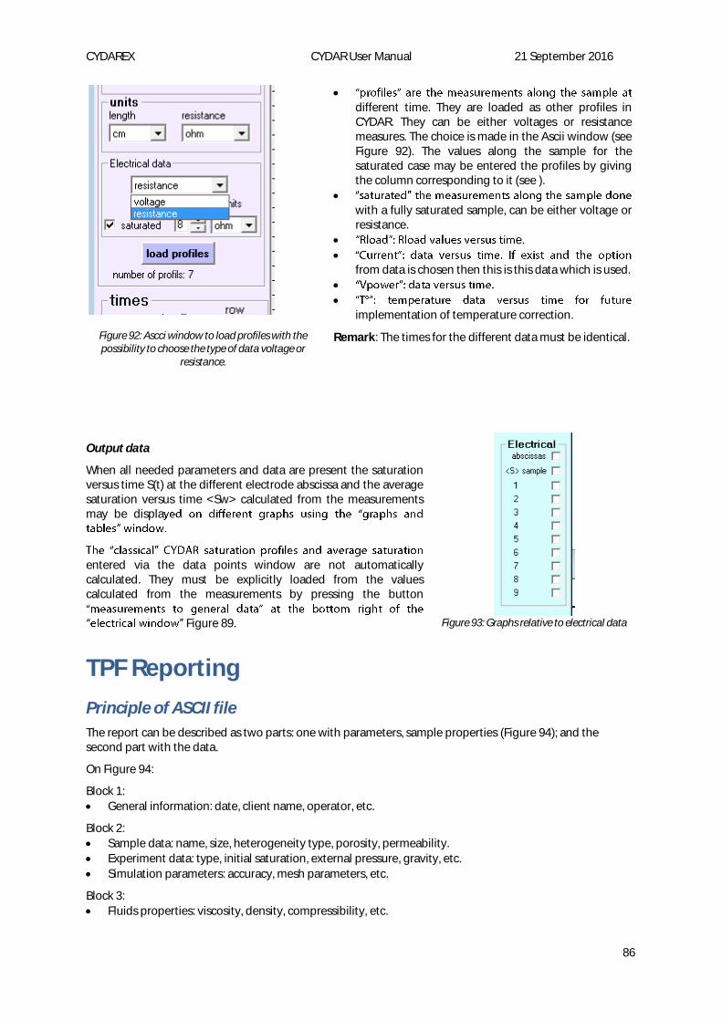
CYDAREX CYDAR User Manual 21 September 2016
86
Figure 92: Ascci window to load profiles with the possibility to choose the type of data voltage or
resistance.
different time. They are loaded as other profiles in CYDAR. They can be either voltages or resistance measures. The choice is made in the Ascii window (see Figure 92). The values along the sample for the saturated case may be entered the profiles by giving the column corresponding to it (see ).
with a fully saturated sample, can be either voltage or resistance.
e.
from data is chosen then this is this data which is used.
implementation of temperature correction.
Remark: The times for the different data must be identical.
Output data
When all needed parameters and data are present the saturation versus time S(t) at the different electrode abscissa and the average saturation versus time <Sw> calculated from the measurements may be displa
entered via the data points window are not automatically calculated. They must be explicitly loaded from the values calculated from the measurements by pressing the button
Figure 89.
Figure 93: Graphs relative to electrical data
TPF Reporting
Principle of ASCII file
The report can be described as two parts: one with parameters, sample properties (Figure 94); and the second part with the data.
On Figure 94:
Block 1:
General information: date, client name, operator, etc.
Block 2:
Sample data: name, size, heterogeneity type, porosity, permeability.
Experiment data: type, initial saturation, external pressure, gravity, etc.
Simulation parameters: accuracy, mesh parameters, etc.
Block 3:
Fluids properties: viscosity, density, compressibility, etc.

CYDAREX CYDAR User Manual 21 September 2016
87
Block 4:
Pc and Kr analytical parameters
The second part summarized data and block time values:
Analytical data of permeability and porosity profiles used in simulation
Block times values: incremental, cumulative time, experimental type inputs (pressures, flow rates, speed) and columns with pressure and volume values allowing easy block times drawing on graphs using template.
pressure, relative permeabilities, delta pressure, outlet volumes, average saturation, volume balance.
With additional data for specific cases as, for example, in centrifuge experiment: Pc(<S>); forbes + splines if calculation have been done.
Figure 94: First part of an ASCII report for an unsteady-state experiment.
Using template:
The main goal of the ASCII report is to be easily imported in spreadsheet programs like OpenOffice or Microsoft Excel. Complex layouts (with graphs, colors, company logo) can then be created using templates. Figure 95 shows a template example.
When using Templates with TPF, relative permeabilities should be plotted with 30 points, and time unit in Block Times should be the same as graph units.
BLOCK 1
BLOCK 2
BLOCK 3
BLOCK 4
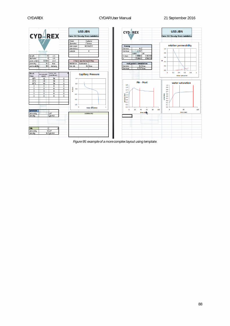
CYDAREX CYDAR User Manual 21 September 2016
88
Figure 95: example of a more complex layout using template.

CYDAREX CYDAR User Manual 21 September 2016
89
Curve Fitting Tool
The Curve Fitting tool, accessed through CYDAR main window (pg. 26), is an independent module that gives access to CYDAR fitting functions, data manipulation, and allows several calculations.
Figure 96: Curve Fitting tools
main window.
information
Load Data (Ascii) loading, editing, or fitting (page 45).
modify data points
edit points pg. 16).
Once data are entered curve fittingdescribe on pg. 17.
Figure 97: View window.
Once data are entered and fitted, the View menu gives access to additional graphs.
CYDAREX CYDAR User Manual 21 September 2016
90
Appendices
Numerical methods Depending on the modules, numerical calculations are based either on explicit or implicit methods.
Explicit methods calculate the state of a system at a later time from the state of the system at the current time, while implicit methods find a solution by solving an equation involving both the current state of the system and the later one.
Mathematically, if Y(t) is the current system state and we want to find Y(t t t t is a small time step), then, for an explicit method:
𝑌(𝑡 + Δ𝑡) = 𝐹(𝑌(𝑡))
while for an implicit method one solves an equation:
𝐺(𝑌(𝑡), 𝑌(𝑡 + Δ𝑡)) = 0
Newton-Raphson and Euler are two examples of powerful methods used to solve implicit schemes in CYDAR.
Newton-Raphson method:
Flow equation can be written as 𝐅(𝑡) = 0 and then the system can be solved with the Newton-Raphson iterative method.
In one dimension, the Newton-Raphson Algorithm to solve 𝑓(𝑥) = 0 is:
First guess: 𝑥0, 𝑘 = 0
Newton-Raphson loop until ‖𝑥𝑘+1 − 𝑥𝑘‖ < 휀:
Solve ∂𝑓(𝑥𝑘)
∂𝑥 Δ𝑥 = −𝑓(𝑥𝑘)
𝑥𝑘+1 = 𝑥𝑘 + Δ𝑥 𝑘: = 𝑘 + 1
The solution is the last 𝑥𝑘+1.
Remark:
It exists different convergence criteria like the relative error ‖𝑥𝑘+1 − 𝑥𝑘‖ < 휀 𝑥𝑘 or on the residual as follow 𝑓(𝑥𝑘) = 휀 𝑓(𝑥0). The choice of the difference, ‖𝑥𝑘+1 − 𝑥𝑘‖ < 휀, as exit test is based on empirical work done over several boundary, initial and experimental conditions.
Euler implicit:
equation:
∂𝑦(𝑡)
∂𝑡= 𝑓(𝑦(𝑡))
The purpose is then to use the finite difference:
∂𝑦
∂𝑡=
(𝑦𝑛+1 − 𝑦𝑛)
𝛿𝑡
and to solve iteratively, with a Newton-Raphson method for instance:
𝑦𝑛+1 = 𝑦𝑛 + 𝛿𝑡 𝑓(𝑦𝑛+1)

CYDAREX CYDAR User Manual 21 September 2016
91
Transient permeability module:
The flow equation is ∂𝜑 𝜌
∂𝑡+ ∇(𝜌 𝐔) = 0 and can be written in term of pressure in one dimension as follow on
each grid:
𝜑(𝑃) 𝑐(𝑃)∂𝑃
∂𝑡+
∂𝜑(𝑃)
∂𝑡+ 𝑈(𝑃) 𝑐(𝑃)
∂𝑃
∂𝑥+
∂𝑈(𝑃)
∂𝑥= 0 ⇔ 𝑓(𝑡, 𝑥) = 0
Because this is solved on each grid, we have a non linear system to solve 𝐹 = 0 Then P and F are vector of
length n (n being the number of grids): 𝑃 = (𝑃1 ⋯ 𝑃𝑖 ⋯ 𝑃𝑛) and 𝐹 = (𝐹1 ⋯ 𝐹𝑖 ⋯ 𝐹𝑛). The
Newton-Raphson algorithm is the same as above with the following system to solve iteratively:
𝑃𝑘+1 = 𝑃𝑘 − 𝐽−1𝑘 𝐹𝑘
With 𝐽−1 the inverse of the Jacobian matrix of 𝐹 in accordance with 𝑃.
Two-phase flow module:
CYDAR has two fully implicit solvers implemented: uncompressible and compressible.
For Two-implicitly.
The well- Saturation) has been removed in the recent version of CYDAR, due to its lack of accuracy.

CYDAREX CYDAR User Manual 21 September 2016
92
Right click menus WHERE ACTION
Input tables
Spreadsheet
removing, inserting lines
Optimization per points:
Kr and Pc tables. Formatting numbers by column
Optimization per points:
Kr and Pc graphs.
Undoing all moves since the beginning of the optimization.
XY Graphs
Loading simulation curve as data points (not available for graphs with several variables displayed
Opening data tables.
Activating Full window display
Axes auto scale

CYDAREX CYDAR User Manual 21 September 2016
93
Shortcuts SHORTCUTS WHERE ACTION
Ctrl+F Text boxes
Input tables and spreadsheet Formatting a number or a column in a table.
Ctrl+Z Optimization per points:
Kr and Pc tables and graphs.
undo the last move only, if no other action has been done
Ctrl+Z Data editing five steps undo stack
Ctrl+Y Optimization per points:
Kr and Pc tables and graphs.
Redo the last undo, if no other action has been done
Ctrl+Y Data editing five steps undo stack
Ctrl+w Any CYDAR Copy to the clipboard
Ctrl + click on Graph Windows Close all graph windows
Shift + click On data point in Graph Shows a window with X-Y values of point

CYDAREX CYDAR User Manual 21 September 2016
94
Troubleshooting Here is an overview of know issues and solutions.
Error message during installation
Depending on the operating system, some messages might occur during installation. Choose the option
the existing file as recommended.
The installation software cannot be launch
If Windows is set to use a Latin alphabet, but the installation software path contents letters from a different alphabet (Hebrew, Arabic, Cyrillic), the installation program might not be able to access the installation files.
If the installation software cannot be launch, it is recommended to use only Latin letters in its path.
If the user name contents non-Latin letters, you can create a temporary user, and run the installation software from the temporary user. Once installed, CYDAR should run without problems even if non-Latin letters are present.
Installation software gets stuck
Under Windows 8 or Windows 10
If the with an Internet connection, as Windows 8 or 10 might be installing additional components needed for the installation.
Also, if the installation blocks icrosoft data access components 2.0 (not
fine.
Text on CYDAR windows is impossible to read
Figure 98.
This problem is due to the fact that the font in each object is too large compare to the object, and the problem can have several origins:
1. In Windows settings, in
2. Under some circumstances, Windows uses a different font for MS sans serif, and this font is slightly larger. The original font can be reset using the registry editor: click on the Windows logo at the bottom left of the screen (formerly the "Start" button), and in the tab "Search for programs In the registry editor, navigate to: HKEY_LOCAL_MACHINE\SOFTWARE\Microsoft\Windows NT\CurrentVersion\Fonts\MS Sans Serif 8,10,12,14,18,24. By double-clicking on the font MS Sans Serif, the value
Note that there is one letter change: a F becoming a E. Press okay, and close the Registry Editor. You need to restart your computer for the change to take effect.
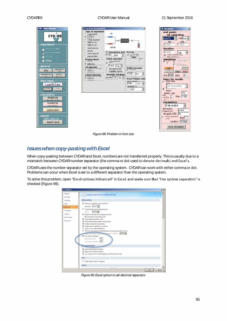
CYDAREX CYDAR User Manual 21 September 2016
95
Figure 98: Problem in font size.
Issues when copy-pasting with Excel
When copy-pasting between CYDAR and Excel, numbers are not transferred properly. This is usually due to a mismatch between CYDAR number separator (the comma or dot used to
CYDAR uses the number separator set by the operating system. CYDAR can work with either comma or dot. Problems can occur when Excel is set to a different separator than the operating system.
To solve this problem, open checked (Figure 99).
Figure 99: Excel option to set decimal separator.

CYDAREX CYDAR User Manual 21 September 2016
96
References 1.
in San Antonio, U.S.A., 05-08 October, 1997.
2. Skjaeveland S.M., Siqveland L.M., Kjosavik A., Hammervold Thomas W.L., Virnovsky G.A.Pressure Correlation for Mixed- (1), February 2000.
3. Aziz K., Settari A., Petroleum Reservoir Simulation, 1979, Applied Science Publishers.
4. Lomeland F., Ebeltoft E. and Thomas H. W, , Reviewed Proceedings of the 2005 International Symposium of the SCA, Abu Dhabi, United Arab Emirates, October 31 - November 2, 2005, SCA 2005-32.
5. Amott, E., "Observations relating to the wettability of porous rock", Transactions of the AIME (219), 156 162, 1959.
6. Leverett, M.C. "Capillary behaviour in porous solids". Transactions of the AIME (142): 159 172, 1941.
7. Klinkenberg, L. (1941). "The permeability of porous media to liquids and gases." Drilling and Production Practice: 200-213.
8. Purcell, W. R. (1949). "Capillary pressures, their measurement using mercury and the calculation of permeability therefrom." Trans AIME (February): 39-48.
9. Johnson, E. F., D. P. Bossler and V.O. Naumann (1959). "Calculation of relative permeability from displacement experiments." Journal of Petroleum Technology (January): 61-63.
10. Jones, S. C. and W. O. Roszelle (1978). "Graphical techniques for determining relative permeability from displacement experiments." Journal of petroleum technology (may): 807-817.
11. Journal of Petroleum Technology, December, 2498-2504, 1981.
12. Dullien, F. A. L., Porous media. Porous structure and fluid transport San Diego, Academic Press Limited, inc., 1992.
13. - Journal of Petroleum Technology, 1983.
14. Rapoport, L. A. and Leas, W. J.: 1953, Properties of linear waterfloods, Trans. AIME 216, 139 148.
15. Jones, F.O. and Owens, W.W.: A laboratory study of low-permeability gas sand, Journal of Petroleum Technology, Sept. 1980, 1631-1640.
16. Fleury, M.: Advances in resistivity measurements using the frim method at reservoir condition, application to carbonates, SCA2003-31, 2003.