cycle-adjusted capital market expectations under black ...robes.fa.ru/docs/v1_2013/08.pdf · 89...

89

Review of Business and Economics Studies Volume 1, Number 1, 2013

Cycle-Adjusted Capital Market Expectations under Black-litterman Framework in global Tactical Asset Allocation*

Anna mikAeLiAnInternational Finance Faculty, Financial University, [email protected]

Abstract. We propose an implementation of Black-Litterman allocation approach with views based on time-varying risk premiums during different phases of business cycle. To obtain views we define 5-phase business cycle taken from US economic history 1979–2012. Then we formulate stylized facts on assets classes’ co-movement during different phases of business cycle and set simplistic rules for generating views based on mentioned facts. To predict phase of cycle we use methodology of 5-phase business cycle prediction based on key macroeconomic indicators analysis. We back-test both approaches and compare them to such classical asset allocation strategies performance, as market-equilibrium portfolio, equal-weighted “naive” diversification, 60/40 and other. We find that Black-Litterman allocation shows superior performance to almost all other allocation strategies during 1980–2011 years.

Аннотация. Вашему вниманию представлено внедрение модели Блэка-Литтермана с входящими данными в виде взглядов относительно доходностей различных классов активов в зависимости от фаз бизнес-цикла. Для формирования этих взглядов мы воспроизводим 5 фаз бизнес-цикла экономики США периода 1979–2012 гг. Далее мы выявляем закономерности динамики классов активов в разные периоды цикла и устанавливаем простые правила формирования взглядов, основанных на этих закономерностях. Для прогнозирования фазы цикла мы используем методологию 5-фазного бизнес-цикла, основанного на анализе ключевых макроэкономических показателей. Мы тестируем оба подхода модели и сравниваем ее с такими классическими стратегиями, как рыночный портфель, равно-взвешенная диверсификация, 60/40 и др. Мы считаем, что диверсификация активов методом Блэка-Литтермана превосходит практически все рассмотренные стратегии в период времени с 1980 по 2011 г.

Key words: Black-Litterman, Markowitz, MVO, MPT, Bayesian prior, posterior, asset allocation, business cycle, Fed recession indicator.

INTROduCTION

The efficiency of asset allocation strategies is one of the core topics of modern financial science at least since seminal work of Brinson et al. (1995) and se-ries of subsequent researches written since then. An evidence of evergreen relevance of this topic is well-known research by Faber (2007), Meucci (2005, 2010), Bekkers et al. (2009), which became one of the most-downloaded research papers on SSRN. Despite well-known flaws in Markowitz approach and theoretically better performance exhibited by Black-Litterman portfolios, no attempt has been made to test and compare historical performance of both approaches in Faber (2007) and Bekkers et al. (2009) style.

The mean-variance optimization (MVO) created by Markowitz became the most widely-used tech-

nique for making investment and asset allocation decisions. The essence of MVO is to create the effi-cient frontier — the set of most optimal portfolios at a given return or level of risk, using historical returns of an asset class. Unfortunately, when investors have tried to use this model, they faced some problems. The main problem of classical Markowitz and his MVO is that the results received are usually unrea-sonable. They occur when, having no constraints, the model chooses large short positions in many assets, and when constrained, it often prescribes “corner” solutions with zero weights in many assets and un-reasonable large weights of assets with small capitali-zation. Thus, the portfolios formed by the MVO are unintuitive and highly concentrated.

Such nature of results is caused by two main prob-lems. First, expected returns are very difficult to esti-

* Учет фаз бизнес-циклов в формировании ожиданий доходности рынков при глобальном тактическом распределении активов в соответствии с моделью Блэка-Литтермана

90


mate and the historical returns used by investors for this purpose provide poor guides to future returns. Second, the optimal portfolio asset weights and cur-rency positions of MVO asset allocation are very sensitive to the return assumptions used. And these two problems compound each other. The model is not able to sort out confident and certain views from simple assumptions and the portfolio it generates has usually a little or even no relation to the views that investor wishes to express.

In order to avoid these problems, Fischer Black and Robert Litterman developed another quantitative ap-proach, known as the Black-Litterman asset allocation model. The Black-Litterman model was first published by Fischer Black and Robert Litterman of Goldman Sachs in an internal Goldman Sachs Fixed Income document in 1990. Their paper was then published in the Journal of Fixed Income in 1991. A longer and richer paper was published in 1992 in the Financial Analysts Journal (FAJ). The model was then discussed in greater details in Bevan and Winkelmann (1998), He and Litterman (1999), Satchell and Scowcroft (2000), Litterman (2003), Idzorek (2004) and Walters (2008). Various applications and extensions of the model were discussed in Beach & Orlov (2007), José Luis Barros Fernandes (2011), Meucci (2010).

The Black-Litterman model combined the CAPM by Sharpe (1964), reverse optimization by Sharpe (1974), mixed estimation by Theil (1971, 1978), the universal hedge ratio/Black’s global CAPM by Black (1989) and Litterman (2003), and mean-variance op-

timization of Markowitz (1952). The model is aimed to overcome the problems of unintuitive, highly-con-centrated portfolios, input-sensitivity, and estima-tion error maximization. It provides both an intuitive portfolio and a clear way to specify investors’ views and to blend the investors’ views with prior informa-tion. The steps of the Black Litterman approach are shown in Figure 1.

But the quite obvious from the first sight conclu-sion of the Black-Litterman’s superiority over the classical Markowitz is not such unambiguous and non-doubtful. It results in more intuitive, diversified portfolios, and most importantly has an opportunity of adding capital market expectations (CME).

First of all, it should be recognized that the proc-ess of generating the CME is rather subjective and it is not evident that adding such expectations im-proves the portfolio performance. The other problem is that no clear understanding exists regarding the validity and relevancy of the historical back-testing within the Black-Litterman or any other model as a tool of portfolio performance estimation. Some other questions and uncertainties are added up with the peculiarities and characteristics of modern financial markets where in addition to traditional debts and equities, a wide variety of alternative asset classes and financial instruments are represented. In other words, it is not unquestionable that the Black-Litter-man with its all above-mentioned advantages is able to outperform other strategies in its risk and return characteristics.

Step 1•Define equilibrium market weights and covariance matrix for all asset classes

Step 2•Back-solve equilibrium expected returns

Step 3•Express views and confidence for each view

Step 4•Calculate the view-adjusted market equilibrium returns

Step 5•Run mean–variance optimization

Inputs for calculating equilibrium expected returns

Form the neutral starting point for formulating expected returns

Reflect the investor’s expectations for various asset classes. The confidence level assigned to each view determines the weight placed on it.

Form the expected return that reflects both market equilibrium and views

Obtain efficient frontier and portfolios

Figure 1. Steps of the Black-Litterman Model*.Source: Maginn, J. L. (2007), “Managing investment portfolios: a dynamic process”, Wiley and Sons.

* See more detail and theoretical background of the Black-Litterman model in Idzorek, Thomas, “A Step-By-Step guide to the Black-Litterman Model, Incorporating User-Specified Confidence Levels.”, Meucci, Attilio, “The Black-Litterman Approach: Original Model and Extensions.”

91


METHOd

The main idea of this research is to assess the Black-Litterman model, its capability to fulfill the initial purposes incumbent on it and to create better per-forming portfolios in modern financial markets’ con-ditions. The testing is to be implemented in several stages as follows:

1. Develop mechanical method of generating CME;

2. Find the source of “ideal post-hoc” CME, which supports us with such expectations as if we had a perfect knowledge about the existing and future mar-ket conditions. This source is needed because a high probability of mistakes exist when the expectations are developed by using the above-chosen mechanical method; using the “ideal” CME we will have an op-portunity to assess the confidence of the mechanical method;

3. Test the classical Markowitz, the Black-Litter-man without views, the Black-Litterman with “ad hoc” and “post hoc” views and other classical alterna-tive strategies of asset allocation, based on the histor-ical dataset. Among other strategies tested there are simple 60/40 stock/bond allocation, adapted 60/40 al-location, based on the market capitalizations weights allocation (market portfolio), equally-weighted allo-cation.

The main assumption of the research is that the fundamental macro-indicators, showing the stage of the business cycle in where the economy is at a point of time, are the main sources of CME. It is generally known that different asset classes act differently de-pending on the phase of the business cycle. Thus, to generate CME we should define the patterns of asset classes’ behavior in different phases of business cycle.

The research is limited by the time horizon and the country analyzed. The testing will be done for the US national economy and financial markets, the time horizon is 33 years (since 1979). Asset classes and their proxies used in testing are as follows:

Domestic fixed income:• Government bonds — 10-Year Treasury Con-

stant Maturity Rate;• Corporate bonds — Moody’s Seasoned AAA Cor-

porate Bond Yield;Domestic equity:• Large-caps — S&P 500 Total Return Index;• Small-caps — Russell 2000 Total Return Index;Commodities — S&P Goldman Sachs Commodity

Total Return Index;Real estate — NAREIT US Real Estate Return

Index;Gold — historical gold prices.

BuSINESS CyClE

We analyzed the United States business cycle and connected its phases to the asset classes’ returns and risks, trying to find the relation between the economy conditions, caused by the business cycle phase, and the asset classes’ risks and returns during that phase. The time horizon analyzed was divided according to the phases of business cycle based on two main indi-cators: the NBER Recession Indicator and the Term Spread between long and short-term FED rates.

The NBER-based division has 5 phases — initial recovery, early upswing, late upswing, slowdown and recession. To find the beginning and ending points of these phases we took quarterly time series of US GDP growth rates, Output Gap, CPI, Sentiments, Initial Claims, Payrolls and NBER Recession Indicator. But this method of division is good only in historical test-ing, as its main indicators are lagging.

The second method, based on Term Spread, tries to predict the business cycle phases. This method is very hypothetical, because no single interpretation of the term spreads’ values exists. Thus, we made our own assumptions of interpreting the probability val-ues (which are the main concept of the method) in business cycle predicting. For each of these methods separate sets of views were developed (for more de-tails see Appendix 1).

CREATINg SPECIFIC INPuTS FOR BlACK-lITTERMAN MOdEl

Views. As mentioned above, we have analyzed the business cycle of US to derive views about asset class-es’ behavior during its different phases. Using two methods (the NBER Recession Indicator-based and the Term Spread-based) we divided the US economy history into periods of different business phases. As a result, we have two types of business cycle divisions, so we will have two sets of views correspondingly.

Also, we made the assets classes’ analysis over the same time horizon (1979–2012). In order to generate views for the Black-Litterman, we must combine that analysis with the business cycle divisions. It means that now we must analyze assets’ quarterly returns and risks with respect to the phases of business cycle. In other words, we must find out the regularities in assets classes behavior over the cycle phases, formulate them and ex-plore as a way of constructing more effective portfolio.

Table 2 contains mean quarterly returns and standard deviations for each NBER Recession Indica-tor–based business cycle phases.

We can now see that in Recessions Russell has the greatest return (5.57%), while the S&P GSCI has

92


a maximum negative return and a highest standard deviation (18.10%). Rationally it can be explained by existence of risk-seeking investors, who are trying to get high returns and are ready to take risk even dur-ing recession, and are choosing Small-caps as the one having less of standard deviation and high rate of re-turn.

In the Initial Recovery REITs are totally beating Gold as during last cycles the economy started its re-covery with the growth of the real estate market.

As for the Early Upswing the Russell is outper-forming S&P500, which is an evidence of growing confidence and a desire to switch to equities as more risky assets in order to have greater returns. The Late Upswing is characterized by the same sen-timents but with the desire to switch to less risky equities, which is S&P 500. Thus, in Late Upswing Large-caps have higher returns than Small-caps. Summarizing all the above ideas, the following views are specified in Table 3.

The figure under each view is an absolute measure of the view. Thus the first view asserts that in Reces-sion Russell’s quarterly return is 8% greater than the one of S&P GSCI.

The same views will be used to the business cy-cle phases’ breakup under the Term-Spread meth-od. Nevertheless, the final views’ vectors under

different methods of business cycle breakup will differ from each other due to the differences in the breakups.

Market capitalizations. Using the market capi-talization weights in asset allocation is one of the main distinctions of the Black-Litterman model from classic Markowitz. As we are analyzing the pe-riod since 1979, we must back-up each asset class’ market-cap history for the same time horizon. The market capitalization history dataset is rather dif-ficult to find. Mainly, the sources give annual data, which is not matching our criteria of quarterly time series. The mission is complicated not only by the long and quarterly frequency history needed, but also by the fact that such asset classes as bonds and gold do not have a clear measure of their market capitalizations. Taking all this into consideration, the quarterly time series of asset classes’ market capitalizations since 1979 till 2012 has been derived by following ways:

• The market capitalization of S&P500, Russell 2000 and FTSE NAREIT are calculated having at least one market cap value of the index at any moment of time horizon since 1979;

• The market capitalization of 10-Year Treasuries and AAA Corporate Bonds is measured by the value of open market interest;

mean stdev mean stdev mean stdev mean stdev mean stdev10‐Y Bonds 2.00% 1.07% 1.77% 0.82% 1.66% 0.81% 1.63% 0.44% 2.19% 0.87%AAA 2.35% 0.90% 2.09% 0.70% 1.95% 0.70% 1.88% 0.41% 2.42% 0.71%SP500 1.40% 11.53% 2.82% 8.77% 3.47% 5.89% 4.48% 6.60% ‐2.95% 6.57%Russell 5.57% 15.11% 6.72% 10.42% 4.14% 8.11% 3.29% 9.05% ‐3.44% 9.50%Gsachs ‐3.11% 18.10% 2.07% 6.92% 2.68% 6.92% 3.26% 9.83% 5.28% 17.26%Gold 0.39% 9.44% 0.38% 7.44% 1.20% 4.95% 1.71% 6.53% 5.16% 16.14%NAREIT 2.00% 15.21% 6.36% 6.25% 3.91% 5.12% 2.70% 6.74% ‐1.50% 5.75%

Asset Classrec initial recovery early upswing late upswing slow down

Table 2. Asset Classes Mean Returns and Standard Deviations in Different Phases of the US Business Cycle.

Table 3. The Views Regarding the Asset Classes’ Returns

Asset Classes Recession Initial Recovery Early upswing late upswing Slowdown

10-y Bonds

AAA

SP500 RUSS > SP 1.5%

SP > RUSS 1.5%

Russell RUS > GSachs 8%

gsachs

gold REIT > GOLD 6%

GOLD > REIT 6%

NAREIT

93


• As a measure of the gold’s market capitalization the value of the total investable gold of US institu-tions is taken;

• The market capitalization of S&P GSCI is calcu-lated by taking its structure at any moment of time. Having the weights of its constituents at a given moment, the value of open interests and the price of each futures contract, the market capitalization is estimated for that date. Then the same procedure is done with the S&P 500 and other simple price in-dexes.

Input assumptions and constraints. In addition to views specified, the Black-Litteman needs other input assumptions. For our Black-Litterman portfo-lios the following assumptions and constraints have been set:

• The value of parameter τ = 0,025;• Trading only long, no short positions allowed;• The risk-free interest rate is zero;• The starting point is the 27-th quarter of the

period analyzed (1986 quarter 1). This assumption is made in order to supply the models with some history of returns as an input.

Having the historical returns, market capitaliza-tions, views and assumptions, we can form all the Black-Litterman portfolios.

THE PORTFOlIOS PERFORMANCE ANAlySIS

In our testing we will compare the Black-Litterman portfolios with the ones of Markowitz, Market port-folio, Equally-weighted portfolio, simple 60/40 stock/bond portfolio, adapted 60/40 stock/bond port-folio.

The Black-Litterman model allows us to construct two types of portfolios: with views specified and with-out any views. At the same time the Black-Litterman portfolio without views differs from classical Markow-

itz as it takes into consideration the market capitali-zation weights of each asset class in the portfolio and uses equilibrium returns.

For our test we will use both these approaches and create two groups of Black-Litterman portfolios:

• The Black-Litterman Equilibrium Returns port-folios without views;

• The Black-Litterman with views specified port-folios. As we have two series of views (NBER-based and FED rates spread-based) the Black-Litterman portfolio with views will be divided into two groups:

■ The NBER-based views Black-Litterman;■ The Fed-based views Black-Litterman;

From the variety of portfolios on the efficient frontier for each type of Black-Litterman model we will take 5 portfolios:

■ the minimum risk portfolio (minrisk);■ the maximum risk portfolio (maxrisk);■ the medium risk portfolio (midrisk);■ the middle between minimum and medium

risk portfolio (minmidrisk);■ the middle between medium and maximum

risk portfolio (midmaxrisk);Such choice of portfolios will simplify further

analysis of the models by comparing corresponding risk-level portfolios created by different asset alloca-tion models and define which of them is better at dif-ferent risk levels.

The same method is used in Markowitz’ portfo-lios, which will also be subdivided by the risk interval.

The Market Portfolio is the portfolio which al-locates asset classes basing on their market capitali-zations. The weight of an asset class is determined by the ratio of its market capitalization to the total market capitalization. The reallocations are also done with respect to changes in market capitalizations.

A 60/40 stock/bond asset allocation is appropri-ate or at least is a starting point for an average inves-

Figure 2. Historical Weights of Market Portfolio.

94


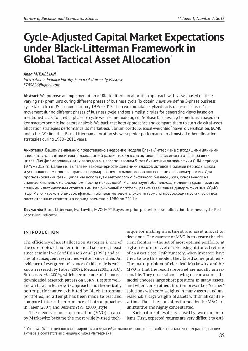
tor’s asset allocation. From periods predating modern portfolio theory to the present, this asset allocation has been suggested as a neutral (neither highly ag-gressive nor conservative) asset allocation. The eq-uities allocation is viewed as supplying a long-term growth foundation, the fixed-income allocation as supplying risk-reduction benefits. If the stock and bond allocations are themselves diversified, an overall diversified portfolio should result.

Our 60/40 portfolio will consist of:• S&P500 and Russell 2000 each with the weights

of 30%, summing up to 60% of stocks;• 10-Year Government and AAA Corporate Bonds

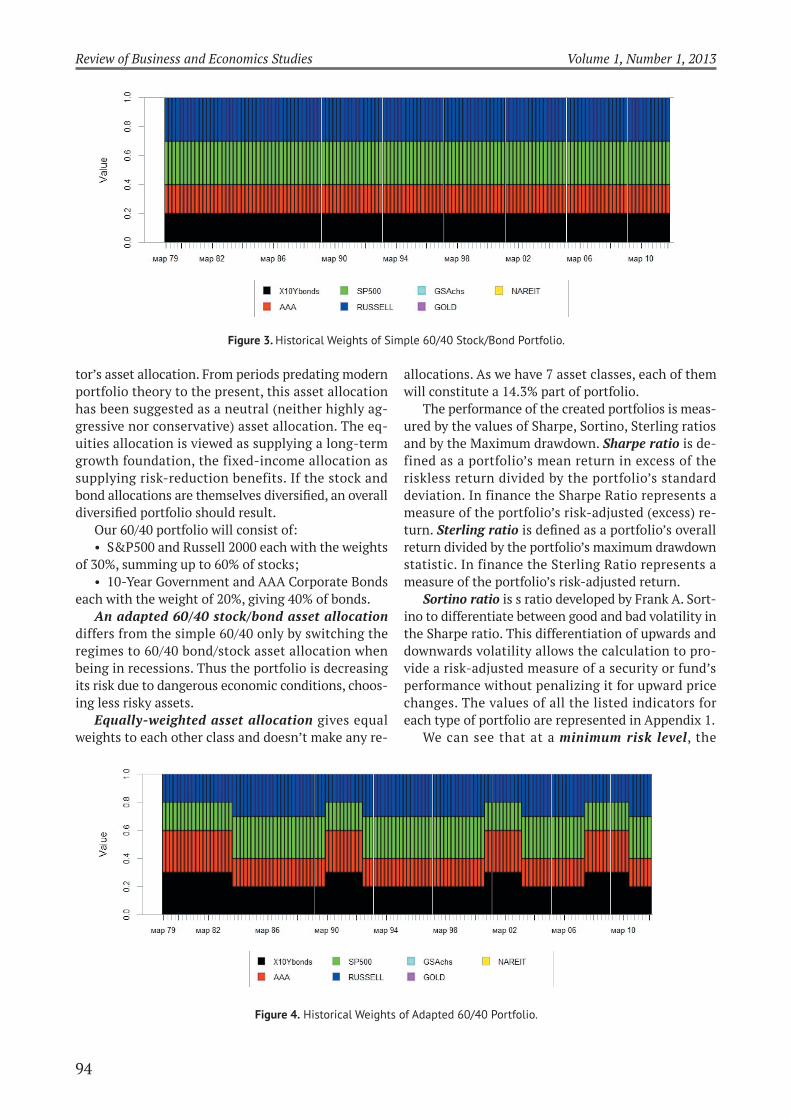
each with the weight of 20%, giving 40% of bonds.An adapted 60/40 stock/bond asset allocation

differs from the simple 60/40 only by switching the regimes to 60/40 bond/stock asset allocation when being in recessions. Thus the portfolio is decreasing its risk due to dangerous economic conditions, choos-ing less risky assets.

Equally-weighted asset allocation gives equal weights to each other class and doesn’t make any re-

allocations. As we have 7 asset classes, each of them will constitute a 14.3% part of portfolio.

The performance of the created portfolios is meas-ured by the values of Sharpe, Sortino, Sterling ratios and by the Maximum drawdown. Sharpe ratio is de-fined as a portfolio’s mean return in excess of the riskless return divided by the portfolio’s standard deviation. In finance the Sharpe Ratio represents a measure of the portfolio’s risk-adjusted (excess) re-turn. Sterling ratio is defined as a portfolio’s overall return divided by the portfolio’s maximum drawdown statistic. In finance the Sterling Ratio represents a measure of the portfolio’s risk-adjusted return.

Sortino ratio is s ratio developed by Frank A. Sort-ino to differentiate between good and bad volatility in the Sharpe ratio. This differentiation of upwards and downwards volatility allows the calculation to pro-vide a risk-adjusted measure of a security or fund’s performance without penalizing it for upward price changes. The values of all the listed indicators for each type of portfolio are represented in Appendix 1.

We can see that at a minimum risk level, the

Figure 3. Historical Weights of Simple 60/40 Stock/Bond Portfolio.

Figure 4. Historical Weights of Adapted 60/40 Portfolio.

95


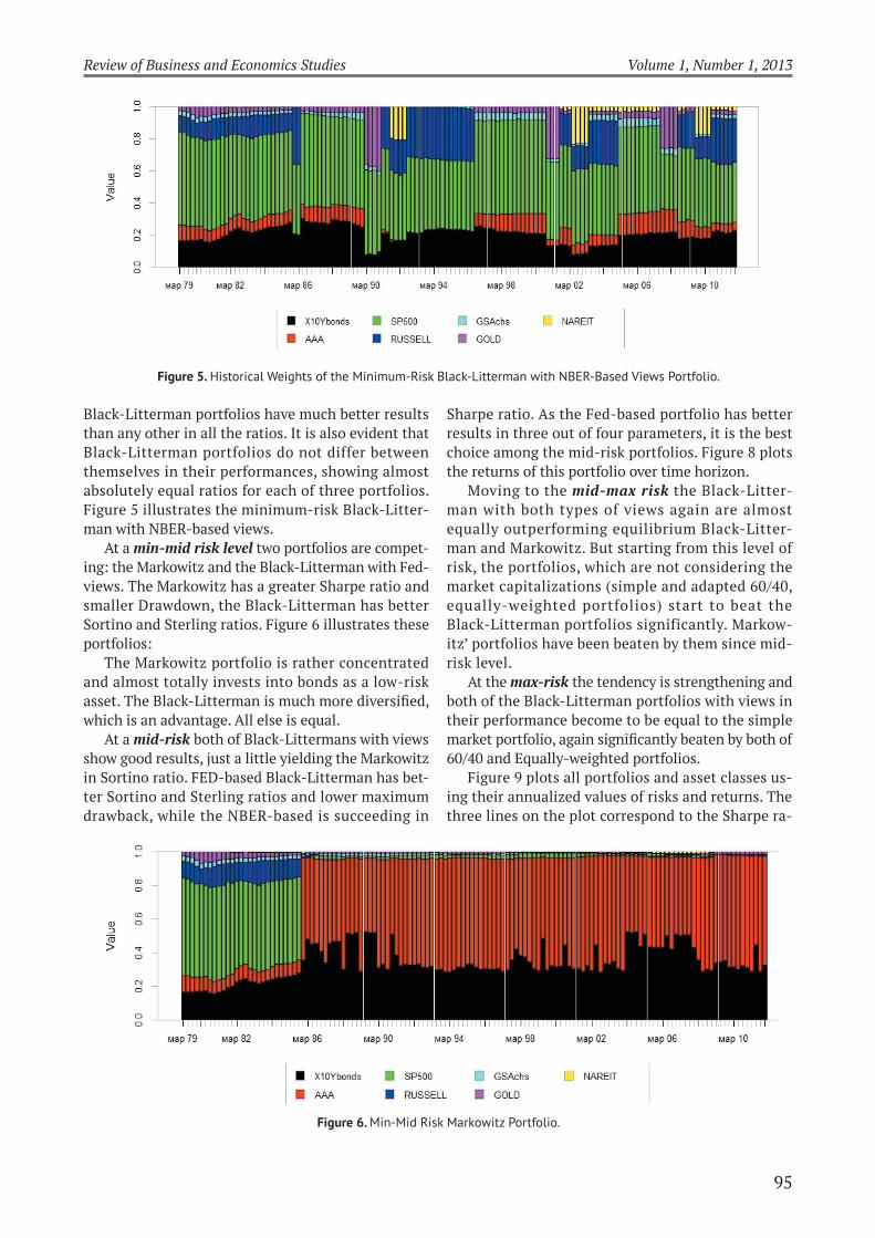
Black-Litterman portfolios have much better results than any other in all the ratios. It is also evident that Black-Litterman portfolios do not differ between themselves in their performances, showing almost absolutely equal ratios for each of three portfolios. Figure 5 illustrates the minimum-risk Black-Litter-man with NBER-based views.

At a min-mid risk level two portfolios are compet-ing: the Markowitz and the Black-Litterman with Fed-views. The Markowitz has a greater Sharpe ratio and smaller Drawdown, the Black-Litterman has better Sortino and Sterling ratios. Figure 6 illustrates these portfolios:

The Markowitz portfolio is rather concentrated and almost totally invests into bonds as a low-risk asset. The Black-Litterman is much more diversified, which is an advantage. All else is equal.

At a mid-risk both of Black-Littermans with views show good results, just a little yielding the Markowitz in Sortino ratio. FED-based Black-Litterman has bet-ter Sortino and Sterling ratios and lower maximum drawback, while the NBER-based is succeeding in

Sharpe ratio. As the Fed-based portfolio has better results in three out of four parameters, it is the best choice among the mid-risk portfolios. Figure 8 plots the returns of this portfolio over time horizon.

Moving to the mid-max risk the Black-Litter-man with both types of views again are almost equally outperforming equilibrium Black-Litter-man and Markowitz. But starting from this level of risk, the portfolios, which are not considering the market capitalizations (simple and adapted 60/40, equally-weighted portfolios) start to beat the Black-Litterman portfolios significantly. Markow-itz’ portfolios have been beaten by them since mid-risk level.

At the max-risk the tendency is strengthening and both of the Black-Litterman portfolios with views in their performance become to be equal to the simple market portfolio, again significantly beaten by both of 60/40 and Equally-weighted portfolios.

Figure 9 plots all portfolios and asset classes us-ing their annualized values of risks and returns. The three lines on the plot correspond to the Sharpe ra-

Figure 5. Historical Weights of the Minimum-Risk Black-Litterman with NBER-Based Views Portfolio.

Figure 6. Min-Mid Risk Markowitz Portfolio.

96


tios. The left line is the line of Sharpe ratio = 3, the middle –2 and the Sharpe ratio of the right line is equal to 1.

From the Figure 9 we may conclude that the Black-Litterman portfolios of the min-mid risk have almost equal risk/return and thus the same attractiveness. The higher risk level portfolios of Black-Litterman and Markowitz show that the NBER-based Black-Lit-terman has the highest return level. The Markowitz with the same level of risk shows lower returns that an equilibrium Black-Litterman.

gENERAl CONCluSIONS

1. At the minimum risk level the views are not signifi-cant. All of three Black-Litterman portfolios are beat-ing other portfolios and are more effective and diver-sified. The values of all the ratios are almost equal for Black-Litterman models with views and without them, which means that views specified do not play a significant role at the minimum level of risk;

2. With the increase of the risk level the significance of views increases too. At the min-mid and mid-risk levels the Black-Litterman portfolios with views start to show much better results than the Black-Litterman without ones;

3. At the middle risk levels the NBER-based Black-Litterman model is the most effective portfolio;

4. At the high risk levels the portfolios not based on market capitalization show better results. Passing the mid-max point, the performance of the Black Litter-man portfolios starts to decline. At this level of risk the portfolios, which do not take the market capi-talization (adapted 60/40, equally-weighted and sim-ple 60/40) start to beat the Black-Litterman portfolios;

5. At the highest level of risk the Black-Litterman portfolios are similar by their performance to the simple market portfolio;

6. The Black-Litterman model beats Markowitz MVO at any level of risk;

7. The Fed term spread method is a precise tool for business cycle predicting.

Figure 7. Min-Mid Risk Black-Litterman with FED-Based Views Portfolio.

Figure 8. Mid-Risk FED-Based Black-Litterman Portfolio’s Historical Returns.

97


REFERENCES

Ammann, M. & Zimmerman, H. (2001), “Tracking Error and Tacti-

cal Asset Allocation”, Financial Analysts Journal 57 (2).

Beach, S.L. & Orlov, A.G. (2007), “An application of the Black–Lit-

terman model with EGARCH-M-derived views for international

portfolio management”, Financial Markets and Portfolio Manage-

ment 21 (2), 147–166.

Bekkers, N., Doeswijk, R. & Lam, T. (2009), “Strategic asset alloca-

tion: Determining the optimal portfolio with ten asset classes”,

Available at SSRN 1368689, 1–33.

Bevan, A. & Winkelmann, K. (1998), “Using the Black-Litterman

Global AssetAllocation Model: Three Years of Practical Experi-

ence.” Fixed Income Research, Goldman, Sachs & Company, De-

cember 1998.

Black, F. & Litterman, R. (1992), “Global Portfolio Optimization,

Financial Analysts Journal 48, 28–43.

Black, F. (1993), “Beta and return”, Journal of Portfolio Management

20, 8–18.

Black, F. (1972), “Capital Market Equilibrium with Restricted Bor-

rowing”, Journal of Business 45 (3), 444–455.

Black, F., Jensen M. C. & Scholes, M. (1972), The Capital Asset Pric-

ing Model: Some Empirical: Tests. Studies in the Theory of Capital

Markets, New York: Praeger Publishers.

Brinson, G.P., Hood, L.R. & Beebower, G.L. (1995), “Determi-

nants of portfolio performance”, Financial Analysts Journal,

133–138.

Campbell, J. & Shiller, R. (1991), “‘Yield Spreads and Interest Rate

Movements””, Review of Economic Studies 58 (3), 495–514.

Chatrath, A. & Liang, Y. (1998), “‘REITs and Inflation: A Long-Run

Perspective””, Journal of Real Estate Research 16 (3).

Chow, G., Jacquier, E., Kritzman, M. & Lowry, K. (1999), “Optimal

Portfolios in Good Times and Bad”, Financial Analysts Journal 55

(3), 65–73.

Christopherson, Jon, and Paul Greenwood, ““Equity Styles and

Why They Matter.”” Journal ofInvestment Consulting. Vol. 1, No.

1: 21–36, 2004.

Estrella, A., Mishkin, F. (1988), “Predicting U. S. Recessions: Finan-

cial Variables as Leading Indicators”, Review of Economics and

Statistics 80 (1), 45–61.

Faber, M.T. (2007), “A quantitative approach to tactical asset alloca-

tion”, Journal of Wealth Management.

Fama, E. & French, K. (1988), “Business Cycles and the Behavior of

Metals Prices”, Journal of Finance 43 (5), 1075–1093.

Fama, E.& French, K. (1992), “The Cross-Section of Expected Stock

Returns””, Journal of Finance 47 (2), 427–465.

Fama, E. & French K. (1996), “Multifactor Explanations of Asset

Pricing Anomalies”, Journal of Finance 51 (1), 55–84.

French, K. & Craig W. (2003), “The Treynor Capital Asset Pricing

Model”, Journal of Investment Management 1 (2), 60–72.

He, G. & Litterman, R. (1999), “The Intuition Behind Black-Litter-

man Model Portfolios”, Goldman Sachs Asset Management Work-

ing paper.

Idzorek, T. (2005), “A Step-By-Step guide to the Black-Litterman

Model, Incorporating User-Specified Confidence Levels”, Work-

ing paper.

Grinold, R., & Kroner, K. (2002), “The Equity Risk Premium”, Invest-

ment Insights from Barclays Global Investors 5 (3).

Grinold, R. & Kahn, R. (1995), Active Portfolio Management, Chicago,

IL: Probus Publications.

Kitchin, J. (1923), “Cycles and Trends in Economic Factors”, Review

of Economics.

Markowitz, H. (1952), “‘Portfolio Selection”, Journal of Finance 7 (1),

77–91.

Markowitz, H. (1959), Portfolio Selection: Efficient Diversification of

Investments, New Haven: Yale University Press.

Markowitz, H. (1984), “The Two Beta Trap”, Journal of Portfolio

Management 10 (1), 12–20.

Figure 9. Annualized Assets’ Risk/Ratio.

98


Meucci, A. (2010), “The Black-Litterman Approach: Original Model

and Extensions”, The Encyclopedia of Quantitative Finance, Wiley.

Meucci, A. (2005), “Beyond Black-Litterman: views on non-normal

markets”, Working paper, available at SSRN 848407.

Merton, R. (1969), “Life Time Portfolio Selection Under Uncertain-

ty: The Continuous Time Case”, Review of Economics and Statis-

tics 51, 247–257.

Merton, R. (1973), “An Intertemporal Capital Asset Pricing Model”,

Econometrica 41 (5), 867–887.

Mitchell, W. (1954), “Business Cycles, the Problem and Its Setting”

New York: National Bureau of Economic Research.

Moore, G. H. (1983), Business Cycles, Inflation and Forecasting (2nd

edition), Cambridge: Ballinger Publishing.

Ross, S. (1976), “The arbitrage theory of capital asset pricing”, Jour-

nal of Economic Theory 13 (3),341–360.

Satchell, S. & Scowcroft, A., “A Demystification of the Black-Lit-

terman Model: Managing Quantitative and Traditional Portfolio

Construction”, Journal of Asset Management 1 (2), 138–150.

Sharpe, W., Gordon A. & Jeffery B. (1999), Investments, Upper Sad-

dle River: Prentice Hall.

Sharpe, W. (1966), “Mutual Fund Performance”, Journal of Business

39 (1), 119–138.

Sharpe, William. 1974. “‘Imputing Expected Security Returns From

Portfolio Composition””, Journal of Financial and Quantitative

Analysis. Vol. 9, No. 3: 463–472.

Schumpeter, J. A. (1954), History of Economic Analysis, London:

George Allen & Unwin.

Theil, H. (1971), Principles of Econometrics, Wiley and Sons.

Tobin, J. (1958), “Liquidity preference as behavior towards risk”,

The Review of Economic Studies 25 (2).

Tsay, R. S. (1998), “Outliers, level shifts, and variance changes in

time series”, Journal of Forecasting 7, 1–20.

Walters, J. (2008), “The Black-Litterman Model in Detail”, Working

paper.

Yamarone, R. (2004), “The trader’s guide to key economic indica-

tors “, 2004.

Appendix 1The NBER Recession based Phases of US Business Cycle (1979–2012)

Period (year/quarter) The Phase of Business Cycle

duration (months) Business Cycle

Beginning End

— 1979/q3 Late upswing N/A, 9 months of data analyzed

Partially completed business cycle with “double-dip recession”, 47 months long1979/q4 1980/q1 Slowdown 6

1980/q2 1980/q3 Recession 6

1980/q4 1981/q1 Initial recovery 6

1981/q2 1981/q3 Slowdown 6

1981/q4 1982/q2 Recession 15

1983/q1 1983/q2 Initial recovery 6 Completed business cycle, 99 months long1983/q3 1985/q4 Early upswing 30

1986/q1 1989/q3 Late upswing 45

1989/q4 1990/q3 Slowdown 12


1991/q2 1992/q1 Initial recovery 12 Completed business cycle, 126 months long1992/q2 1996/q1 Early upswing 48


2000/q3 2001/q1 Slowdown 9


2002/q1 2002/q4 Initial recovery 12 Completed business cycle,80 months long2003/q1 2004/q3 Early upswing 21


2008 q1 2008 q1 Slowdown 3

2008 q2 2009 q2 Recession 15

2009 q3 2010 q1 Initial recovery 9 Partially completed business cycle, 33 months long

99


Appendix 2Portfolios Performance Ratios

Risk level Portfolio Type Performance Measure

Sharpe Sortino drawdown Sterling

MinRisk Markowitz 0.91508 0.37984 0.06033 -0.20212

BL without views 1.61104 0.74600 0.09712 -0.07951

BL with Fedviews 1.61105 0.74601 0.09712 -0.07951

BL with NBER views 1.61105 0.74601 0.09711 -0.07951

Min-Mid Risk Markowitz 1.78132 0.67301 0.06033 -0.16128

BL without views 1.25870 0.50258 0.17814 0.04281

BL with Fed views 1.36454 0.68016 0.10687 0.09777

BL with NBER views 1.37270 0.58016 0.15299 0.08664

Mid Risk Markowitz 0.78269 0.55071 0.17408 0.07451

BL without views 0.92402 0.37467 0.29495 0.12835

BL withFedviews 1.03240 0.54599 0.19073 0.24387


Mid-Max Risk Markowitz 0.64770 0.28283 0.42647 0.16262

BL without views 0.70015 0.30785 0.40261 0.16212

BL with Fedviews 0.77926 0.43046 0.24847 0.29179


Max-Risk Markowitz 0.53607 0.25828 0.50351 0.23920

BL without views 0.48386 0.23571 0.45803 0.25308

BL withFedviews 0.80986 0.27794 0.43217 0.28791


Market Portfolio 0.78950 0.32778 0.37746 0.17837

Simple 60/40 0.94971 0.42914 0.29340 0.17458

Adapted 60/40 1.14333 0.54928 0.18787 0.23243

Equally-weighted 1.10059 0.40897 0.31221 0.01307

NBER recession indicator is posted quarterly by Business Cycle Dating Committee of US National Bureau for Economic Research (NBER), an official arbiter of recessions for US economy. Com-mittee uses no predefined rule but members’ judgment based on macro data, to mark periods of recession with two-quarters lag. Indicator may be equal to 0 or 1, with 1 indicating recession period.

FED spread recession indicator is published monthly by New York FED and varies between 0 and 100, showing probability of US economy falling into recession during next month. This is leading index, calculated from spread between market price for short- and long-term US government debt. Method for calcula-tion, as well as all accompanying materials, is in open access on the site of New York FED.

Black-Litterman and Meucci techniques are “add-ons” to famous Markowitz MVO approach to portfolio optimization. Black-Litterman approach allows to blend portfolio manager forecasts with prior returns distribution, based on assumptions of market returns normality, and uses blended returns as inputs for Markowitz optimisation procedure. Meucci’s approach fur-ther extends that of Black-Litterman, by allowing returns to be non-normal.

Ensemble learning is class of decision making algorithms, com-bining forecasts of ensemble of “weak predictors” ensemble (i.e. any other decision making models with low predictive ability) to make one “strong predictor” with higher predictive performance

than any of individual predictors, comprising it. Ensemble learn-ing is believed to produce better results when applied to com-plex, non-stationary processes and high dimensional data.

Corporate sustainability reporting is optional non-financial reporting (often prepared as part of part of mandatory financial reporting), supplying organisation’s stakeholders with addi-tional information about social, environmental and governance performance of corporation. By preparing sustainability reports organisation shows to investors and mass media its awareness of bidirectional impacts of organisational activity and various aspects of sustainability, as well as internalizes its commitment to sustainable development and engaging stakeholders.

Real options is a valuation technique, which allows to consider simultaneously several paths or scenarios of development of some basic (for valued object) parameter and the flexibility of object’s manager to react in real time to some particular path or scenario being realized. For example, applying real options approach to problem of finding fair rent price for gold mine al-lows to account for varying gold price and flexibility of mine’s management to cease mine operation when gold price is low, and install new equipment when gold price is high. Real options approach have numerous applications in valuing endeavors in R&D, licensing, energy, mining, policymaking, etc. Real options are not traded derivatives; rather it is approach to valuation of objects, the fair value (of benefit from realization) of which could be conceptually tied to price of some underlying asset and de-pends heavily on decisions taken as reaction to the price change.

TERMINOLOGY

cycle-adjusted capital market expectations under black ...robes.fa.ru/docs/v1_2013/08.pdf · 89...

Documents