cven 489-501: special topics in mixing and transport processes
TRANSCRIPT
CVEN 489-501: Special Topics in
Mixing and Transport Processes in the
Environment
Engineering – Lectures
By
Scott A. Socolofsky &
Gerhard H. Jirka
5th Edition, 2005
Coastal and Ocean Engineering Division
Texas A&M University
M.S. 3136
College Station, TX 77843-3136

2
Recommended Reading
Journal Articles
Journals are a major source of information on Environmental Fluid Mechanics. Major journals
include Environmental Fluid Mechanics, published by Kluwer, the Journal of Hydraulic Engi-
neering published by the American Society of Civil Engineers (ASCE), the Journal of Hydraulic
Research published by the International Association of Hydraulic Engineering and Research
(IAHR), Limnology and Oceanography published by the American Society of Limnology and
Oceanography (ASLO), Physics of Fluids, published by the American Physics Society (APS),
and the Journal of Fluid Mechanics published by Cambridge University Press, among many
others. These are all available through the Texas A&M University library: newer articles are
available through on-line subscriptions, and older articles (usually before 1995) are available in
bound volumes in the library stacks.
Supplemental Textbooks
The material for this course is also treated in a number of other books; in particular, the
following supplementary texts are recommended:
Fischer, H. B., List, E. G., Koh, R. C. Y., Imberger, J. & Brooks, N. H. (1979), Mixing in
Inland and Coastal Waters, Academic Press, New York, NY.
Hemond, H. F. & Fechner-Levy, E. J. (2000), ‘Chemical Fate and Transport in the Environ-
ment, Academic Press, San Diego, CA.
Condensed Bibliography
The following books are also recommended for in-depth study of individual topics:
Acheson, D. J. (1990), Elementary Fluid Dynamics, Oxford Applied Mathematics and Com-
puting Science Series, Clarendon Press, Oxford, England.
Csanady, G. T. (1973), Turbulent Diffusion in the Environment, D. Reidel Publishing Com-
pany, Dordrecht, Holland.
VI Recommended Reading
Kundu, P. K. & Cohen, I. M. (2002), Fluid Mechanics, 2nd Edition, Academic Press, San
Diego, CA.
Mei, C. C. (1997), Mathematical Analysis in Engineering, Cambridge University Press, Cam-
bridge, England.
Rutherford, J. C. (1994), River Mixing, John Wiley & Sons, Chichester, England.
van Dyke, M. (1982), An Album of Fluid Motion, The Parabolic Press, Stanford, CA.
Wetzel, R. G. (1983), Limnology, Saunders Press, Philadelphia, PA.

Preface
Environmental Fluid Mechanics (EFM) is the study of motions and transport processes in earth’s
hydrosphere and atmosphere on a local or regional scale (up to 100 km). At larger scales, the
Coriolis force due to earth’s rotation must be considered, and this is the topic of Geophysical
Fluid Dynamics. Sticking purely to EFM in this book, we will be concerned with the interaction
of flow, mass and heat with man-made facilities and with the local environment.
This text is the first Part in a two-part book to accompany a two-semester course in Envi-
ronmental Fluid Mechanics. In this Part, Mixing and Transport Processes in the Environment,
passive diffusion is treated by introducing the transport equation and its application in a range
of unstratified water bodies. Passive diffusion refers to mixing processes that occur due to ran-
dom motions and that have no direct feedback on the dynamics of the fluid motion. The second
Part, Stratified Flow and Buoyant Mixing, covers the dynamics of stratified fluids and transport
under active diffusion. Active diffusion relates to mixing processes that have a direct feedback on
the equations of motion due to changes in the density of the carrier fluid. This first Part is ap-
propriate for senior level undergraduate students; whereas, the second Part is more appropriate
for first-year graduate students.
The text is designed to compliment existing text books in water quality, air quality, and
transport. A unique feature of this text is that most of the mathematics is written out in
sufficient detail that all of the equations should be derivable (and checkable!) by the reader.
This fifth edition adds more homework problems to each chapter and expands the text and
explanations in each chapter.
The chapters are all organized in a similar fashion. Following the chapter heading, the first
two paragraphs orient the chapter in the context of the other chapters and outline the material
to be covered. In the first section of the chapter, general, background information is covered
that is needed to fully understand the contents of the chapter. The middle sections develop
the appropriate theory and present the mathematical derivations. The final section in each
chapter presents applications of the material to engineering practice. At the end of each chapter,
a summary section highlights the key points and a set of exercises are presented as possible
homework problems. The book contains a single references section and index.
This book was compiled from several sources, including the lecture notes developed by Ger-
hard H. Jirka for courses offered at Cornell University and the University of Karlsruhe, lecture
notes developed by Scott A. Socolofsky for courses taught at the University of Karlsruhe and
Texas A&M University, and notes taken by Scott A. Socolofsky in various fluid mechanics courses
offered at the Massachusetts Institute of Technology (MIT), the University of Colorado, and the
Copyright c© 2004 by Scott A. Socolofsky and Gerhard H. Jirka. All rights reserved.

VIII Preface
University of Stuttgart, including courses taught by E. Eric Adams, Helmut Kobus, Ole S. Mad-
sen, Chiang C. Mei, Heidi M. Nepf, Harihar Rajaram, Joe Ryan, and Ain Sonin. Many thanks
goes to these mentors who have taught this enjoyable subject.
Comments, questions, and corrections on this script can always be addressed per E-Mail to
the address: [email protected].
College Station, Scott A. Socolofsky
January 2005 Gerhard H. Jirka

Contents
1. Concepts, Definitions, and the Diffusion
Equation . . . . . . . . . . . . . . . . . . . . . . . . . . . . . . . . . . . . . . . . . . . . . . . . . . . . . . . . . . . . . . . . . . . 1
1.1 Concepts, Significance and Definitions . . . . . . . . . . . . . . . . . . . . . . . . . . . . . . . . . . . . . . 1
1.1.1 Example Problems . . . . . . . . . . . . . . . . . . . . . . . . . . . . . . . . . . . . . . . . . . . . . . . . . . 2
1.1.2 Expressing Concentration . . . . . . . . . . . . . . . . . . . . . . . . . . . . . . . . . . . . . . . . . . . . 6
1.1.3 Dimensional analysis . . . . . . . . . . . . . . . . . . . . . . . . . . . . . . . . . . . . . . . . . . . . . . . . 7
1.2 Diffusion . . . . . . . . . . . . . . . . . . . . . . . . . . . . . . . . . . . . . . . . . . . . . . . . . . . . . . . . . . . . . . . . 8
1.2.1 Fickian diffusion . . . . . . . . . . . . . . . . . . . . . . . . . . . . . . . . . . . . . . . . . . . . . . . . . . . . 9
1.2.2 Diffusion coefficients . . . . . . . . . . . . . . . . . . . . . . . . . . . . . . . . . . . . . . . . . . . . . . . . 11
1.2.3 Diffusion equation . . . . . . . . . . . . . . . . . . . . . . . . . . . . . . . . . . . . . . . . . . . . . . . . . . 11
1.2.4 One-dimensional diffusion equation . . . . . . . . . . . . . . . . . . . . . . . . . . . . . . . . . . . 14
1.3 Similarity solution to the one-dimensional diffusion equation . . . . . . . . . . . . . . . . . . . 14
1.3.1 Interpretation of the similarity solution . . . . . . . . . . . . . . . . . . . . . . . . . . . . . . . . 19
1.4 Application: Diffusion in a lake . . . . . . . . . . . . . . . . . . . . . . . . . . . . . . . . . . . . . . . . . . . . 20
Exercises . . . . . . . . . . . . . . . . . . . . . . . . . . . . . . . . . . . . . . . . . . . . . . . . . . . . . . . . . . . . . . . . . . . . 22
2. Advective Diffusion Equation . . . . . . . . . . . . . . . . . . . . . . . . . . . . . . . . . . . . . . . . . . . . . . 29
2.1 Derivation of the advective diffusion equation . . . . . . . . . . . . . . . . . . . . . . . . . . . . . . . . 29
2.1.1 The governing equation . . . . . . . . . . . . . . . . . . . . . . . . . . . . . . . . . . . . . . . . . . . . . 29
2.1.2 Point-source solution . . . . . . . . . . . . . . . . . . . . . . . . . . . . . . . . . . . . . . . . . . . . . . . . 31
2.1.3 Incompressible fluid . . . . . . . . . . . . . . . . . . . . . . . . . . . . . . . . . . . . . . . . . . . . . . . . . 32
2.1.4 Rules of thumb . . . . . . . . . . . . . . . . . . . . . . . . . . . . . . . . . . . . . . . . . . . . . . . . . . . . . 33
2.2 Solutions to the advective diffusion equation . . . . . . . . . . . . . . . . . . . . . . . . . . . . . . . . . 34
2.2.1 Initial spatial concentration distribution . . . . . . . . . . . . . . . . . . . . . . . . . . . . . . . 34
2.2.2 Fixed concentration . . . . . . . . . . . . . . . . . . . . . . . . . . . . . . . . . . . . . . . . . . . . . . . . . 35
2.2.3 Fixed, no-flux boundaries . . . . . . . . . . . . . . . . . . . . . . . . . . . . . . . . . . . . . . . . . . . . 37
2.3 Application: Diffusion in a Lake . . . . . . . . . . . . . . . . . . . . . . . . . . . . . . . . . . . . . . . . . . . . 39
2.4 Application: Fishery intake protection . . . . . . . . . . . . . . . . . . . . . . . . . . . . . . . . . . . . . . 40
Exercises . . . . . . . . . . . . . . . . . . . . . . . . . . . . . . . . . . . . . . . . . . . . . . . . . . . . . . . . . . . . . . . . . . . . 42
3. Mixing in Rivers: Turbulent Diffusion
and Dispersion . . . . . . . . . . . . . . . . . . . . . . . . . . . . . . . . . . . . . . . . . . . . . . . . . . . . . . . . . . . . . 51
3.1 Turbulence and mixing . . . . . . . . . . . . . . . . . . . . . . . . . . . . . . . . . . . . . . . . . . . . . . . . . . . . 51
Copyright c© 2004 by Scott A. Socolofsky and Gerhard H. Jirka. All rights reserved.
X Contents
3.1.1 Mathematical descriptions of turbulence . . . . . . . . . . . . . . . . . . . . . . . . . . . . . . . 53
3.1.2 The turbulent advective diffusion equation . . . . . . . . . . . . . . . . . . . . . . . . . . . . . 55
3.1.3 Turbulent diffusion coefficients in rivers . . . . . . . . . . . . . . . . . . . . . . . . . . . . . . . . 56
3.2 Longitudinal dispersion . . . . . . . . . . . . . . . . . . . . . . . . . . . . . . . . . . . . . . . . . . . . . . . . . . . 59
3.2.1 Derivation of the advective dispersion equation . . . . . . . . . . . . . . . . . . . . . . . . . 60
3.2.2 Calculating longitudinal dispersion coefficients . . . . . . . . . . . . . . . . . . . . . . . . . . 64
3.3 Application: Dye studies . . . . . . . . . . . . . . . . . . . . . . . . . . . . . . . . . . . . . . . . . . . . . . . . . . 67
3.3.1 Preparations . . . . . . . . . . . . . . . . . . . . . . . . . . . . . . . . . . . . . . . . . . . . . . . . . . . . . . . 67
3.3.2 River flow rates . . . . . . . . . . . . . . . . . . . . . . . . . . . . . . . . . . . . . . . . . . . . . . . . . . . . 70
3.3.3 River dispersion coefficients . . . . . . . . . . . . . . . . . . . . . . . . . . . . . . . . . . . . . . . . . . 71
3.4 Application: Dye study in Cowaselon Creek . . . . . . . . . . . . . . . . . . . . . . . . . . . . . . . . . . 71
Exercises . . . . . . . . . . . . . . . . . . . . . . . . . . . . . . . . . . . . . . . . . . . . . . . . . . . . . . . . . . . . . . . . . . . . 74
4. Physical, Chemical, and Biological
Transformations . . . . . . . . . . . . . . . . . . . . . . . . . . . . . . . . . . . . . . . . . . . . . . . . . . . . . . . . . . . 81
4.1 Concepts and definitions . . . . . . . . . . . . . . . . . . . . . . . . . . . . . . . . . . . . . . . . . . . . . . . . . . 81
4.1.1 Physical transformation . . . . . . . . . . . . . . . . . . . . . . . . . . . . . . . . . . . . . . . . . . . . . 82
4.1.2 Chemical transformation . . . . . . . . . . . . . . . . . . . . . . . . . . . . . . . . . . . . . . . . . . . . 82
4.1.3 Biological transformation . . . . . . . . . . . . . . . . . . . . . . . . . . . . . . . . . . . . . . . . . . . . 83
4.2 Reaction kinetics . . . . . . . . . . . . . . . . . . . . . . . . . . . . . . . . . . . . . . . . . . . . . . . . . . . . . . . . . 83
4.2.1 First-order reactions . . . . . . . . . . . . . . . . . . . . . . . . . . . . . . . . . . . . . . . . . . . . . . . . 85
4.2.2 Second-order reactions . . . . . . . . . . . . . . . . . . . . . . . . . . . . . . . . . . . . . . . . . . . . . . 86
4.2.3 Higher-order reactions . . . . . . . . . . . . . . . . . . . . . . . . . . . . . . . . . . . . . . . . . . . . . . . 88
4.3 Incorporating transformation with the advective-
diffusion equation . . . . . . . . . . . . . . . . . . . . . . . . . . . . . . . . . . . . . . . . . . . . . . . . . . . . . . . . 89
4.3.1 Homogeneous reactions: The advective-reacting
diffusion equation . . . . . . . . . . . . . . . . . . . . . . . . . . . . . . . . . . . . . . . . . . . . . . . . . . . 89
4.3.2 Heterogeneous reactions: Reaction boundary conditions . . . . . . . . . . . . . . . . . . 90
4.4 Application: Wastewater treatment plant . . . . . . . . . . . . . . . . . . . . . . . . . . . . . . . . . . . . 91
Exercises . . . . . . . . . . . . . . . . . . . . . . . . . . . . . . . . . . . . . . . . . . . . . . . . . . . . . . . . . . . . . . . . . . . . 93
5. Boundary Exchange: Air-Water and
Sediment-Water Interfaces . . . . . . . . . . . . . . . . . . . . . . . . . . . . . . . . . . . . . . . . . . . . . . . . . 95
5.1 Boundary exchange . . . . . . . . . . . . . . . . . . . . . . . . . . . . . . . . . . . . . . . . . . . . . . . . . . . . . . . 95
5.1.1 Exchange into a stagnant water body . . . . . . . . . . . . . . . . . . . . . . . . . . . . . . . . . 96
5.1.2 Exchange into a turbulent water body . . . . . . . . . . . . . . . . . . . . . . . . . . . . . . . . . 97
5.1.3 Lewis-Whitman model . . . . . . . . . . . . . . . . . . . . . . . . . . . . . . . . . . . . . . . . . . . . . . 98
5.1.4 Film-renewal model . . . . . . . . . . . . . . . . . . . . . . . . . . . . . . . . . . . . . . . . . . . . . . . . . 98
5.2 Air/water interface . . . . . . . . . . . . . . . . . . . . . . . . . . . . . . . . . . . . . . . . . . . . . . . . . . . . . . . 100
5.2.1 General gas transfer . . . . . . . . . . . . . . . . . . . . . . . . . . . . . . . . . . . . . . . . . . . . . . . . . 101
5.2.2 Aeration: The Streeter-Phelps equation . . . . . . . . . . . . . . . . . . . . . . . . . . . . . . . . 102
5.3 Sediment/water interface . . . . . . . . . . . . . . . . . . . . . . . . . . . . . . . . . . . . . . . . . . . . . . . . . . 104
Contents XI
5.3.1 Adsorption/desorption in disperse aqueous systems . . . . . . . . . . . . . . . . . . . . . 107
Exercises . . . . . . . . . . . . . . . . . . . . . . . . . . . . . . . . . . . . . . . . . . . . . . . . . . . . . . . . . . . . . . . . . . . . 110
6. Atmospheric Mixing . . . . . . . . . . . . . . . . . . . . . . . . . . . . . . . . . . . . . . . . . . . . . . . . . . . . . . . 113
6.1 Atmospheric turbulence . . . . . . . . . . . . . . . . . . . . . . . . . . . . . . . . . . . . . . . . . . . . . . . . . . . 113
6.1.1 Atmospheric planetary boundary layer (APBL) . . . . . . . . . . . . . . . . . . . . . . . . . 114
6.1.2 Turbulent properties of a neutral APBL . . . . . . . . . . . . . . . . . . . . . . . . . . . . . . . 114
6.1.3 Effects of buoyancy . . . . . . . . . . . . . . . . . . . . . . . . . . . . . . . . . . . . . . . . . . . . . . . . . 117
6.2 Turbulent mixing in three dimensions . . . . . . . . . . . . . . . . . . . . . . . . . . . . . . . . . . . . . . . 118
6.3 Atmospheric mixing models . . . . . . . . . . . . . . . . . . . . . . . . . . . . . . . . . . . . . . . . . . . . . . . 119
6.3.1 Near-field solution . . . . . . . . . . . . . . . . . . . . . . . . . . . . . . . . . . . . . . . . . . . . . . . . . . 121
6.3.2 Far-field solution . . . . . . . . . . . . . . . . . . . . . . . . . . . . . . . . . . . . . . . . . . . . . . . . . . . 121
Exercises . . . . . . . . . . . . . . . . . . . . . . . . . . . . . . . . . . . . . . . . . . . . . . . . . . . . . . . . . . . . . . . . . . . . 122
7. Water Quality Modeling . . . . . . . . . . . . . . . . . . . . . . . . . . . . . . . . . . . . . . . . . . . . . . . . . . . 125
7.1 Systematic approach to modeling . . . . . . . . . . . . . . . . . . . . . . . . . . . . . . . . . . . . . . . . . . . 125
7.1.1 Modeling methodology . . . . . . . . . . . . . . . . . . . . . . . . . . . . . . . . . . . . . . . . . . . . . . 125
7.1.2 Issues of scale and complexity . . . . . . . . . . . . . . . . . . . . . . . . . . . . . . . . . . . . . . . . 127
7.1.3 Data availability . . . . . . . . . . . . . . . . . . . . . . . . . . . . . . . . . . . . . . . . . . . . . . . . . . . . 129
7.2 Simple water quality models . . . . . . . . . . . . . . . . . . . . . . . . . . . . . . . . . . . . . . . . . . . . . . . 129
7.2.1 Advection dominance: Plug-flow reactors . . . . . . . . . . . . . . . . . . . . . . . . . . . . . . 130
7.2.2 Diffusion dominance: Continuously-stirred tank reactors . . . . . . . . . . . . . . . . . 131
7.2.3 Tanks-in-series models . . . . . . . . . . . . . . . . . . . . . . . . . . . . . . . . . . . . . . . . . . . . . . . 132
7.3 Numerical models . . . . . . . . . . . . . . . . . . . . . . . . . . . . . . . . . . . . . . . . . . . . . . . . . . . . . . . . 134
7.3.1 Coupling hydraulics and transport . . . . . . . . . . . . . . . . . . . . . . . . . . . . . . . . . . . . 134
7.3.2 Numerical methods . . . . . . . . . . . . . . . . . . . . . . . . . . . . . . . . . . . . . . . . . . . . . . . . . 135
7.3.3 Role of matrices . . . . . . . . . . . . . . . . . . . . . . . . . . . . . . . . . . . . . . . . . . . . . . . . . . . . 136
7.3.4 Stability problems . . . . . . . . . . . . . . . . . . . . . . . . . . . . . . . . . . . . . . . . . . . . . . . . . . 136
7.4 Model testing . . . . . . . . . . . . . . . . . . . . . . . . . . . . . . . . . . . . . . . . . . . . . . . . . . . . . . . . . . . . 136
7.4.1 Conservation of mass . . . . . . . . . . . . . . . . . . . . . . . . . . . . . . . . . . . . . . . . . . . . . . . . 137
7.4.2 Comparison with analytical solutions . . . . . . . . . . . . . . . . . . . . . . . . . . . . . . . . . . 137
7.4.3 Comparison with field data . . . . . . . . . . . . . . . . . . . . . . . . . . . . . . . . . . . . . . . . . . 137
Exercises . . . . . . . . . . . . . . . . . . . . . . . . . . . . . . . . . . . . . . . . . . . . . . . . . . . . . . . . . . . . . . . . . . . . 139
A. Point-source Diffusion in an Infinite Domain:
Boundary and Initial Conditions . . . . . . . . . . . . . . . . . . . . . . . . . . . . . . . . . . . . . . . . . . . 141
B. Solutions to the Advective Reacting
Diffusion Equation . . . . . . . . . . . . . . . . . . . . . . . . . . . . . . . . . . . . . . . . . . . . . . . . . . . . . . . . . 145
B.1 Instantaneous point source . . . . . . . . . . . . . . . . . . . . . . . . . . . . . . . . . . . . . . . . . . . . . . . . 145
B.1.1 Steady, uni-directional velocity field . . . . . . . . . . . . . . . . . . . . . . . . . . . . . . . . . . . 145
B.1.2 Fluid at rest with isotropic diffusion . . . . . . . . . . . . . . . . . . . . . . . . . . . . . . . . . . 145
XII Contents
B.1.3 No-flux boundary at z = 0 . . . . . . . . . . . . . . . . . . . . . . . . . . . . . . . . . . . . . . . . . . . 146
B.1.4 Steady shear flow . . . . . . . . . . . . . . . . . . . . . . . . . . . . . . . . . . . . . . . . . . . . . . . . . . . 146
B.2 Instantaneous line source . . . . . . . . . . . . . . . . . . . . . . . . . . . . . . . . . . . . . . . . . . . . . . . . . . 146
B.2.1 Steady, uni-directional velocity field . . . . . . . . . . . . . . . . . . . . . . . . . . . . . . . . . . . 146
B.2.2 Truncated line source . . . . . . . . . . . . . . . . . . . . . . . . . . . . . . . . . . . . . . . . . . . . . . . 147
B.3 Instantaneous plane source . . . . . . . . . . . . . . . . . . . . . . . . . . . . . . . . . . . . . . . . . . . . . . . . 147
B.4 Continuous point source . . . . . . . . . . . . . . . . . . . . . . . . . . . . . . . . . . . . . . . . . . . . . . . . . . 147
B.4.1 Times after injection stops . . . . . . . . . . . . . . . . . . . . . . . . . . . . . . . . . . . . . . . . . . . 148
B.4.2 Continuous injection . . . . . . . . . . . . . . . . . . . . . . . . . . . . . . . . . . . . . . . . . . . . . . . . 148
B.4.3 Continuous point source neglecting
longitudinal diffusion . . . . . . . . . . . . . . . . . . . . . . . . . . . . . . . . . . . . . . . . . . . . . . . . 148
B.4.4 Continuous point source in uniform flow with
anisotropic, non-homogeneous turbulence . . . . . . . . . . . . . . . . . . . . . . . . . . . . . . 149
B.4.5 Continuous point source in shear flow with
non-homogeneous, isotropic turbulence . . . . . . . . . . . . . . . . . . . . . . . . . . . . . . . . 149
B.5 Continuous line source . . . . . . . . . . . . . . . . . . . . . . . . . . . . . . . . . . . . . . . . . . . . . . . . . . . . 149
B.5.1 Steady state solution . . . . . . . . . . . . . . . . . . . . . . . . . . . . . . . . . . . . . . . . . . . . . . . . 150
B.5.2 Continuous line source neglecting longitudinal
diffusion . . . . . . . . . . . . . . . . . . . . . . . . . . . . . . . . . . . . . . . . . . . . . . . . . . . . . . . . . . . 150
B.6 Continuous plane source . . . . . . . . . . . . . . . . . . . . . . . . . . . . . . . . . . . . . . . . . . . . . . . . . . 150
B.6.1 Times after injection stops . . . . . . . . . . . . . . . . . . . . . . . . . . . . . . . . . . . . . . . . . . . 150
B.6.2 Continuous injection . . . . . . . . . . . . . . . . . . . . . . . . . . . . . . . . . . . . . . . . . . . . . . . . 151
B.6.3 Continuous plane source neglecting
longitudinal diffusion in downstream section . . . . . . . . . . . . . . . . . . . . . . . . . . . 151
B.6.4 Continuous plane source neglecting
decay in upstream section . . . . . . . . . . . . . . . . . . . . . . . . . . . . . . . . . . . . . . . . . . . 151
B.7 Continuous plane source of limited extent . . . . . . . . . . . . . . . . . . . . . . . . . . . . . . . . . . . 152
B.7.1 Semi-infinite continuous plane source . . . . . . . . . . . . . . . . . . . . . . . . . . . . . . . . . . 152
B.7.2 Rectangular continuous plane source . . . . . . . . . . . . . . . . . . . . . . . . . . . . . . . . . . 152
B.8 Instantaneous volume source . . . . . . . . . . . . . . . . . . . . . . . . . . . . . . . . . . . . . . . . . . . . . . . 153
C. Streeter-Phelps Equation . . . . . . . . . . . . . . . . . . . . . . . . . . . . . . . . . . . . . . . . . . . . . . . . . . 155
D. Common Water Quality Models . . . . . . . . . . . . . . . . . . . . . . . . . . . . . . . . . . . . . . . . . . . . 157
D.1 One-dimensional models . . . . . . . . . . . . . . . . . . . . . . . . . . . . . . . . . . . . . . . . . . . . . . . . . . 157
D.1.1 QUAL2E: Enhanced stream water quality model . . . . . . . . . . . . . . . . . . . . . . . 157
D.1.2 HSPF: Hydrological Simulation Program–FORTRAN . . . . . . . . . . . . . . . . . . . 158
D.1.3 SWMM: Stormwater Management Model . . . . . . . . . . . . . . . . . . . . . . . . . . . . . . 158
D.1.4 DYRESM-WQ: Dynamic reservoir water quality model . . . . . . . . . . . . . . . . . . 159
D.1.5 CE-QUAL-RIV1: A one-dimensional, dynamic flow and water quality
model for streams . . . . . . . . . . . . . . . . . . . . . . . . . . . . . . . . . . . . . . . . . . . . . . . . . . 159
D.1.6 ATV Gewassergutemodell . . . . . . . . . . . . . . . . . . . . . . . . . . . . . . . . . . . . . . . . . . . 160
Contents XIII
D.2 Two- and three-dimensional models . . . . . . . . . . . . . . . . . . . . . . . . . . . . . . . . . . . . . . . . 160
D.2.1 CORMIX: Cornell Mixing-Zone Model . . . . . . . . . . . . . . . . . . . . . . . . . . . . . . . . 160
D.2.2 WASP: Water Quality Analysis Simulation Program . . . . . . . . . . . . . . . . . . . . 161
D.2.3 POM: Princeton ocean model . . . . . . . . . . . . . . . . . . . . . . . . . . . . . . . . . . . . . . . . 161
D.2.4 ECOM-si: Estuarine, coastal and ocean model . . . . . . . . . . . . . . . . . . . . . . . . . . 161
Glossary . . . . . . . . . . . . . . . . . . . . . . . . . . . . . . . . . . . . . . . . . . . . . . . . . . . . . . . . . . . . . . . . . . . . . . . 163
References . . . . . . . . . . . . . . . . . . . . . . . . . . . . . . . . . . . . . . . . . . . . . . . . . . . . . . . . . . . . . . . . . . . . . 168
Index . . . . . . . . . . . . . . . . . . . . . . . . . . . . . . . . . . . . . . . . . . . . . . . . . . . . . . . . . . . . . . . . . . . . . . . . . . 171

XIV Contents

1. Concepts, Definitions, and the Diffusion
Equation
Environmental fluid mechanics is the study of fluid mechanical processes that affect the fate and
transport of substances through the hydrosphere and atmosphere at the local or regional scale1
(up to 100 km). In more layman’s terms, environmental fluid mechanics studies how fluids
move substances through the natural environment as they are also transformed. In general,
the substances we may be interested in are mass, momentum or heat. More specifically, mass
can represent any of a wide variety of passive and reactive tracers, such as dissolved oxygen,
salinity, heavy metals, nutrients, and many others. This course and textbook discusses passive
processes affecting the transport of species in a homogeneous natural environment. That is, as
the substance is transported, its presence does not cause a change in the dynamics of the fluid
motion. The book for part 2 of this course, “Stratified Flow and Buoyant Mixing,” incorporates
the effects of buoyancy and stratification to deal with active mixing problems where the fluid
dynamics change in response to the transported substance.
This chapter introduces the concept of mass transfer (transport) and focuses on the physics
of diffusion. Because the concept of diffusion is fundamental to this part of the course, we
single it out here and derive its mathematical representation from first principles through to an
important solution of the governing partial differential equation. The mathematical rigor of this
section is deemed necessary so that the student gains a fundamental and complete understanding
of diffusion and the diffusion equation. This foundation will make the complicated processes
discussed in the remaining chapters tractable and will start to build the engineering intuition
needed to solve problems in environmental fluid mechanics.
1.1 Concepts, Significance and Definitions
Stated simply, environmental fluid mechanics is the study of natural processes that change
concentrations.2
These processes can be categorized into two broad groups: transport and transformation.
Transport refers to those processes which move substances through the hydrosphere and atmo-
sphere by physical means. As an analogy to the postal service, transport is the process by which
a letter goes from one location to another. The postal truck is the analogy for our fluid, and
1 At larger scales we must account for the Earth’s rotation through the Coriolis effect, and this is the subject ofgeophysical fluid dynamics.
2 A glossary at the end of this text provides a list of important terms and their definitions in environmental fluidmechanics (with the associated German term) to help orient the reader to a wealth of new terminology.
Copyright c© 2004 by Scott A. Socolofsky and Gerhard H. Jirka. All rights reserved.

2 1. Concepts, Definitions, and the Diffusion Equation
the letter itself is the analogy for our chemical species. The two primary modes of transport in
environmental fluid mechanics are advection (transport associated with the flow of a fluid) and
diffusion (transport associated with random motions within a fluid). The second process, trans-
formation, refers to those processes that change a substance of interest into another substance.
Keeping with our analogy, transformation is the paper recycling factory that turns our letter
into a shoe box. The two primary modes of transformation are physical (transformations caused
by physical laws, such as radioactive decay) and chemical (transformations caused by chemical
or biological reactions, such as dissolution and respiration).
In engineering practice, environmental fluid mechanics provides the tools to (1) assess the
flow of nutrients and chemicals vital to life through the ecosystem, (2) limit toxicity, and (3)
minimize man’s impact on global climate.
1. Ecosystem Dynamics. Nutrients are food sources used by organisms to generate energy.
Engineers need to know the levels of nutrients and their transformation pathways in order to
predict species populations in freshwater ecosystems, such as the growth and decay of algal
blooms in response to phytoplankton and zooplankton dynamics. Some common nutrients
and vital chemicals are oxygen, carbon dioxide, phosphorus, nitrogen, and an array of heavy
metals, among others.
2. Toxicity. For toxic chemicals, engineers need to understand natural transport and trans-
formation processes to design projects that minimize the probability of occurrence of toxic
concentrations while maintaining an affordable budget. Some common toxic chemicals are
heavy metals (such as iron, zinc, and cadmium), radioactive substances (such as uranium
and plutonium), and poisons and carcinogenic substances (such as PCBs, MTBE, carbon
monoxide, arsenic, and strong acids).
3. Global Climate Change. Some chemical species are also of interest due to their ef-
fects on the global climate system. Some notable substances are the chlorofluorocarbons
(CFCs) which deplete the ozone layer, the greenhouse gases, in particular, carbon dioxide
and methane, which maintain a warm planet, and other substances, such as sulfate aerosols
that affect the Earth’s reflectivity through cloud formation.
It is important to remember that all chemicals are necessary at appropriate levels to sustain
life and that anthropogenic input of chemicals into the hydrosphere is a necessary characteristic
of industrialization. Engineers use environmental fluid mechanics, therefore, to avoid adverse
impacts and optimize the designs of engineering projects and to mitigate the effects of accidents.
1.1.1 Example Problems
Although environmental fluid mechanics addresses basic processes that we are all familiar with
through our natural interaction with the environment (e.g. sensing smoke in a crowded bar),
its application in engineering is not frequently taught and students may find a steep learning
curve in mastering its concepts, terminology, and significance. This problem is compounded by
the fact that a whole new set of equations must be mastered before meaningful design problems
can be addressed. Here, we pause to introduce several typical problems and their relationship

1.1 Concepts, Significance and Definitions 3
Turbulence
Diffusion
Air-flow in
Air-flow out
Gas or
aerosol
release
Fig. 1.1. Schematic of the mixing processes in an enclosed space. A point source of substance is released in thelower left corner of a room. Mixing is caused by flow into and out or the room through the ventilation system andby random motions in the circulating air.
to environmental fluid mechanics to whet the appetite for more detailed study and to give a
context for the derivations that follow.
Indoor air pollution. Chemicals that we come in contact with the most readily are transported
through the air we breath. The two important transport processes are advection (movement
with the air currents generated by wind or by air distribution systems) and diffusion (gradual
spreading of the substance by random motions in the air). This is depicted schematically in
Figure 1.1.
When the anthrax problems in the U.S. Postal Service surfaced shortly after 9/11, there
was a lot of discussion about “weapons grade” anthrax which could be dispersed by the air.
Typical anthrax spores are too heavy to be carried very far by air. However, if anthrax can be
transported by aerosol particles (particles small enough that they have no appreciable settling
velocity), then the threat is much greater. Diffusion, especially turbulent diffusion, as we will
see in Chapter 3, is very efficient at distributing aerosols throughout an enclosed space. In fact,
diffusion is primarily what allows you to smell wet paint, smoke, or a pleasant perfume. If anthrax
could be dispersed through the air, then it could diffuse efficiently throughout enclosed spaces,
greatly increasing the risk that anyone entering the space would be infected.
When engineers design indoor air systems, one thing they are concerned with is the ability of
the system to keep the space well mixed (that is, free of deadzones were contaminants could get
concentrated) and frequently refreshed (new air replacing old). Environmental fluid mechanics
provides the tools to estimate mixing rates and to design better systems. New designs might be
quieter, or use less energy, or rely on natural ventilation generated by temperature differences
between the indoors and outside. The first topics we will cover, diffusion followed by advection,
are directly related to these problems and design issues.
River discharges. Because rivers are readily accessible and efficiently transport chemicals
downstream, they are the primary receiving waters for a whole host of industrial and public
4 1. Concepts, Definitions, and the Diffusion Equation
Industrial
discharge
Natural river
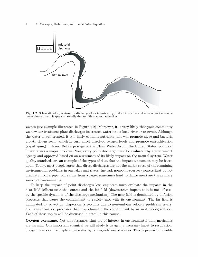
Fig. 1.2. Schematic of a point-source discharge of an industrial byproduct into a natural stream. As the sourcemoves downstream, it spreads laterally due to diffusion and advection.
wastes (see example illustrated in Figure 1.2). Moreover, it is very likely that your community
wastewater treatment plant discharges its treated water into a local river or reservoir. Although
the water is well treated, it still likely contains nutrients that will promote algae and bacteria
growth downstream, which in turn affect dissolved oxygen levels and promote eutrophication
(rapid aging) in lakes. Before passage of the Clean Water Act in the United States, pollution
in rivers was a major problem. Now, every point discharge must be evaluated by a government
agency and approved based on an assessment of its likely impact on the natural system. Water
quality standards are an example of the types of data that the impact assessment may be based
upon. Today, most people agree that direct discharges are not the major cause of the remaining
environmental problems in our lakes and rivers. Instead, nonpoint sources (sources that do not
originate from a pipe, but rather from a large, sometimes hard to define area) are the primary
source of contaminants.
To keep the impact of point discharges low, engineers must evaluate the impacts in the
near field (effects near the source) and the far field (downstream impact that is not affected
by the specific dynamics of the discharge mechanism). The near-field is dominated by diffusion
processes that cause the contaminant to rapidly mix with its environment. The far field is
dominated by advection, dispersion (stretching due to non-uniform velocity profiles in rivers)
and transformation processes that may eliminate the contaminant by natural biodegradation.
Each of these topics will be discussed in detail in this course.
Oxygen exchange. Not all substances that are of interest in environmental fluid mechanics
are harmful. One important chemical we will study is oxygen, a necessary input to respiration.
Oxygen levels can be depleted in water by biodegradation of wastes. This is primarily possible
1.1 Concepts, Significance and Definitions 5
-z
z
Diffusion of oxygen through
air-water interface
High concentration
Low concentration
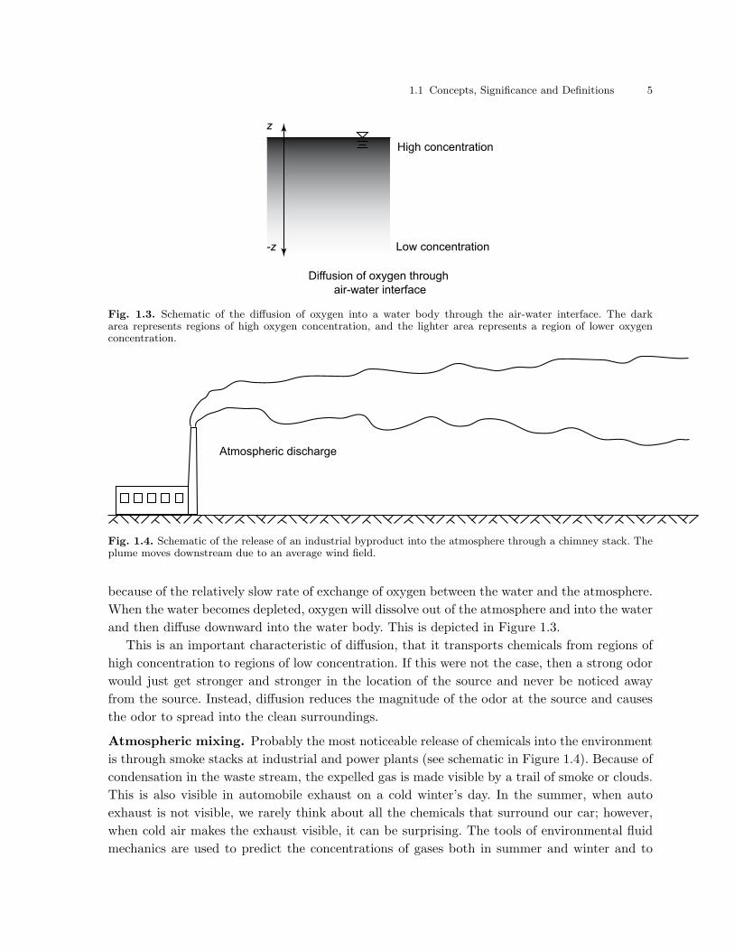
Fig. 1.3. Schematic of the diffusion of oxygen into a water body through the air-water interface. The darkarea represents regions of high oxygen concentration, and the lighter area represents a region of lower oxygenconcentration.
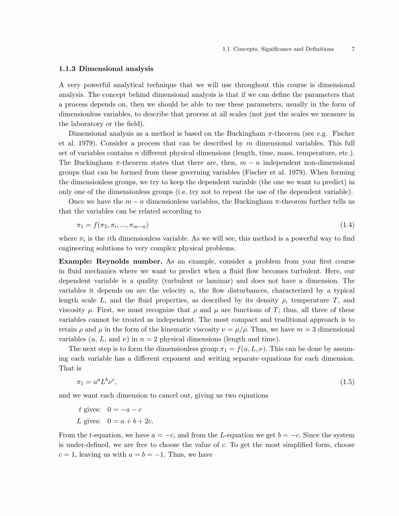
Atmospheric discharge
Fig. 1.4. Schematic of the release of an industrial byproduct into the atmosphere through a chimney stack. Theplume moves downstream due to an average wind field.
because of the relatively slow rate of exchange of oxygen between the water and the atmosphere.
When the water becomes depleted, oxygen will dissolve out of the atmosphere and into the water
and then diffuse downward into the water body. This is depicted in Figure 1.3.
This is an important characteristic of diffusion, that it transports chemicals from regions of
high concentration to regions of low concentration. If this were not the case, then a strong odor
would just get stronger and stronger in the location of the source and never be noticed away
from the source. Instead, diffusion reduces the magnitude of the odor at the source and causes
the odor to spread into the clean surroundings.
Atmospheric mixing. Probably the most noticeable release of chemicals into the environment
is through smoke stacks at industrial and power plants (see schematic in Figure 1.4). Because of
condensation in the waste stream, the expelled gas is made visible by a trail of smoke or clouds.
This is also visible in automobile exhaust on a cold winter’s day. In the summer, when auto
exhaust is not visible, we rarely think about all the chemicals that surround our car; however,
when cold air makes the exhaust visible, it can be surprising. The tools of environmental fluid
mechanics are used to predict the concentrations of gases both in summer and winter and to

6 1. Concepts, Definitions, and the Diffusion Equation
help design exhaust systems, both for your car and for factories, that do not result in toxic
levels. Again, the primary mechanisms we must address are transport (advection and diffusion)
and transformation (reactions).
1.1.2 Expressing Concentration
In order to evaluate how much of a chemical is present in any region of a fluid, we require a
means to measure chemical intensity or presence. This fundamental quantity in environmental
fluid mechanics is called concentration. In common usage, the term concentration expresses a
measure of the amount of a substance within a mixture.
Mathematically, the concentration C is the ratio of the mass of a substance Mi to the total
volume of a mixture V expressed
C =Mi
V. (1.1)
The units of concentration are [M/L3], commonly reported in mg/l, kg/m3, lb/gal, etc. For
one- and two-dimensional problems, concentration can also be expressed as the mass per unit
segment length [M/L] or per unit area, [M/L2].
A related quantity, the mass fraction χ, is the ratio of the mass of a substance Mi to the
total mass of a mixture M , written
χ =Mi
M. (1.2)
Mass fraction is unitless, but is often expressed using mixed units, such as mg/kg, parts per
million (ppm), or parts per billion (ppb).
A popular concentration measure used by chemists is the molar concentration θ. Molar con-
centration is defined as the ratio of the number of moles of a substance Ni to the total volume
of the mixture
θ =Ni
V. (1.3)
The units of molar concentration are [number of molecules/L3]; typical examples are mol/l and
µmol/l. To work with molar concentration, recall that the atomic weight of an atom is reported
in the Periodic Table in units of g/mol and that a mole is 6.022 · 1023 molecules.
The measure chosen to express concentration is essentially a matter of taste. Always use
caution and confirm that the units chosen for concentration are consistent with the equations
used to predict fate and transport. A common source of confusion arises from the fact that mass
fraction and concentration are often used interchangeably in dilute aqueous systems. This comes
about because the density of pure water at 4C is 1 g/cm3, making values for concentration in
mg/l and mass fraction in ppm identical. Extreme caution should be used in other solutions,
as in seawater or the atmosphere, where ppm and mg/l are not identical. The conclusion to be
drawn is: always check your units.
1.1 Concepts, Significance and Definitions 7
1.1.3 Dimensional analysis
A very powerful analytical technique that we will use throughout this course is dimensional
analysis. The concept behind dimensional analysis is that if we can define the parameters that
a process depends on, then we should be able to use these parameters, usually in the form of
dimensionless variables, to describe that process at all scales (not just the scales we measure in
the laboratory or the field).
Dimensional analysis as a method is based on the Buckingham π-theorem (see e.g. Fischer
et al. 1979). Consider a process that can be described by m dimensional variables. This full
set of variables contains n different physical dimensions (length, time, mass, temperature, etc.).
The Buckingham π-theorem states that there are, then, m − n independent non-dimensional
groups that can be formed from these governing variables (Fischer et al. 1979). When forming
the dimensionless groups, we try to keep the dependent variable (the one we want to predict) in
only one of the dimensionless groups (i.e. try not to repeat the use of the dependent variable).
Once we have the m− n dimensionless variables, the Buckingham π-theorem further tells us
that the variables can be related according to
π1 = f(π2, πi, ..., πm−n) (1.4)
where πi is the ith dimensionless variable. As we will see, this method is a powerful way to find
engineering solutions to very complex physical problems.
Example: Reynolds number. As an example, consider a problem from your first course
in fluid mechanics where we want to predict when a fluid flow becomes turbulent. Here, our
dependent variable is a quality (turbulent or laminar) and does not have a dimension. The
variables it depends on are the velocity u, the flow disturbances, characterized by a typical
length scale L, and the fluid properties, as described by its density ρ, temperature T , and
viscosity µ. First, we must recognize that ρ and µ are functions of T ; thus, all three of these
variables cannot be treated as independent. The most compact and traditional approach is to
retain ρ and µ in the form of the kinematic viscosity ν = µ/ρ. Thus, we have m = 3 dimensional
variables (u, L, and ν) in n = 2 physical dimensions (length and time).
The next step is to form the dimensionless group π1 = f(u, L, ν). This can be done by assum-
ing each variable has a different exponent and writing separate equations for each dimension.
That is
π1 = uaLbνc, (1.5)
and we want each dimension to cancel out, giving us two equations
t gives: 0 = −a − c
L gives: 0 = a + b + 2c.
From the t-equation, we have a = −c, and from the L-equation we get b = −c. Since the system
is under-defined, we are free to choose the value of c. To get the most simplified form, choose
c = 1, leaving us with a = b = −1. Thus, we have

8 1. Concepts, Definitions, and the Diffusion Equation
π1 =ν
uL. (1.6)
This non-dimensional combination is just the inverse of the well-known Reynolds number Re;
thus, we have shown through dimensional analysis, that the turbulent state of the fluid should
depend on the Reynolds number
Re =uL
ν, (1.7)
which is a classical result in fluid mechanics.
Example: mixing scales. In environmental fluid mechanics we often want to know how long
it will take for a chemical to mix through a space or how far downstream a chemical will go
before it mixes to a certain size. In this problem we have three parameters: L is the distance over
which the chemical spreads, D is a measure of the rate of diffusion, and t is the time. Although
we have not formally introduced D, it is sufficient now to know that its dimensions are [L2/t]
and that large D give rapid mixing and small D give slow mixing. Thus, we have three variables
and two dimensions (L and t), yielding one non-dimensional number
π1 =Dt
L2. (1.8)
Later, we will see that this number is called the Peclet number.
If we want to know over how large a distance diffusion will spread a chemical in a time t, we
can rearrange the non-dimensional number to solve for length, giving
L ∝√
Dt. (1.9)
This is a classical scaling law in environmental fluid mechanics, and one that we will use fre-
quently. The proportionality constant will change for different geometries, but the scaling rela-
tionship will remain. Hence,√
Dt will be called the diffusion length scale. With this background,
we are now prepared to introduce the important concept of diffusion in more mathematical de-
tail.
1.2 Diffusion
As we have seen, a fundamental transport process in environmental fluid mechanics is diffusion.
Diffusion differs from advection in that it is random in nature (does not necessarily follow a fluid
particle). A well-known example is the diffusion of perfume in an empty room. If a bottle of
perfume is opened and allowed to evaporate into the air, soon the whole room will be scented. We
also know from experience that the scent will be stronger near the source and weaker as we move
away, but fragrance molecules will have wondered throughout the room due to random molecular
and turbulent motions. Thus, diffusion has two primary properties: it is random in nature, and
transport is from regions of high concentration to low concentration, with an equilibrium state
of uniform concentration.

1.2 Diffusion 9
(a.) Initial (b.) Randommotionsdistribution
(c.) Finaldistribution
n
x
n
x0 0
...
Fig. 1.5. Schematic of the one-dimensional molecular (Brownian) motion of a group of molecules illustrating theFickian diffusion model. The upper part of the figure shows the particles themselves; the lower part of the figuregives the corresponding histogram of particle location, which is analogous to concentration.
1.2.1 Fickian diffusion
We just observed in our perfume example that regions of high concentration tend to spread into
regions of low concentration under the action of diffusion. Here, we want to derive a mathematical
expression that predicts this spreading-out process, and we will follow an argument presented
in Fischer et al. (1979).
To derive a diffusive flux equation, consider two rows of molecules side-by-side and centered
at x = 0, as shown in Figure 1.5(a.). Each of these molecules moves about randomly in response
to the temperature (in a random process called Brownian motion). Here, for didactic purposes,
we will consider only one component of their three-dimensional motion: motion right or left
along the x-axis. We further define the mass of particles on the left as Ml, the mass of particles
on the right as Mr, and the probability (transfer rate per time) that a particles moves across
x = 0 as k, with units [T−1].
After some time δt an average of half of the particles have taken steps to the right and half
have taken steps to the left, as depicted through Figure 1.5(b.) and (c.). Looking at the particle
histograms also in Figure 1.5, we see that in this random process, maximum concentrations
decrease, while the total region containing particles increases (the cloud spreads out).
Mathematically, the average flux of particles from the left-hand column to the right is kMl,
and the average flux of particles from the right-hand column to the left is −kMr, where the
minus sign is used to distinguish direction. Thus, the net flux of particles qx is
qx = k(Ml − Mr). (1.10)
For the one-dimensional case we can write (1.10) in terms of concentrations using
Cl = Ml/(δxδyδz) (1.11)
10 1. Concepts, Definitions, and the Diffusion Equation
Cr = Mr/(δxδyδz) (1.12)
where δx is the width, δy is the breadth, and δz is the height of each column. Physically, δx is
the average step along the x-axis taken by a molecule in the time δt. For the one-dimensional
case, we want qx to represent the flux in the x-direction per unit area perpendicular to x; hence,
we will take δyδz = 1. Next, we note that a finite difference approximation for dC/dx is
dC
dx=
Cr − Cl
xr − xl
=Mr − Ml
δx(xr − xl), (1.13)
which gives us a second expression for (Ml − Mr), namely,
(Ml − Mr) = −δx(xr − xl)dC
dx. (1.14)
Taking δx = (xr − xl) and substituting (1.14) into (1.10) yields
qx = −k(δx)2dC
dx. (1.15)
(1.15) contains two unknowns, k and δx. Fischer et al. (1979) argue that since q cannot depend
on an arbitrary δx, we must assume that k(δx)2 is a constant, which we will call the diffusion
coefficient, D. Substituting, we obtain the one-dimensional diffusive flux equation
qx = −DdC
dx. (1.16)
It is important to note that diffusive flux is a vector quantity and, since concentration is expressed
in units of [M/L3], it has units of [M/(L2T)]. To compute the total mass flux rate m, in units
[M/T], the diffusive flux must be integrated over a surface area. For the one-dimensional case
we would have m = Aqx, where A = δyδz.
Generalizing to three dimensions, we can write the diffusive flux vector at a point by adding
the other two dimensions, yielding (in various types of notation)
q = −D
(
∂C
∂x,∂C
∂y,∂C
∂z
)
= −D∇C
= −D∂C
∂xi. (1.17)
Diffusion processes that obey this relationship are called Fickian diffusion, and (1.17) is called
Fick’s law. To obtain the total mass flux rate we must integrate the normal component of q over
a surface area, as in
m =
∫∫
Aq · ndA (1.18)
where n is the unit vector normal to the surface A.
1.2 Diffusion 11
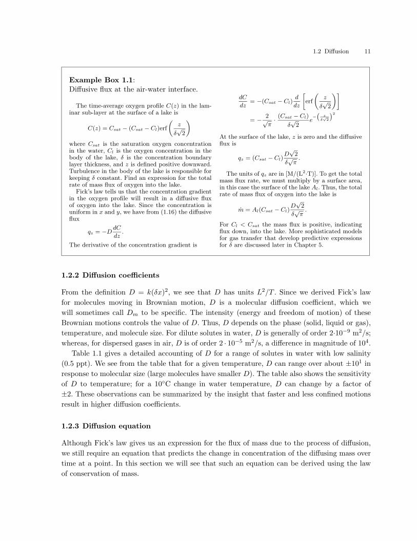
Example Box 1.1:Diffusive flux at the air-water interface.
The time-average oxygen profile C(z) in the lam-inar sub-layer at the surface of a lake is
C(z) = Csat − (Csat − Cl)erf
(
z
δ√
2
)
where Csat is the saturation oxygen concentrationin the water, Cl is the oxygen concentration in thebody of the lake, δ is the concentration boundarylayer thickness, and z is defined positive downward.Turbulence in the body of the lake is responsible forkeeping δ constant. Find an expression for the totalrate of mass flux of oxygen into the lake.
Fick’s law tells us that the concentration gradientin the oxygen profile will result in a diffusive fluxof oxygen into the lake. Since the concentration isuniform in x and y, we have from (1.16) the diffusiveflux
qz = −DdC
dz.
The derivative of the concentration gradient is
dC
dz= −(Csat − Cl)
d
dz
[
erf
(
z
δ√
2
)]
= − 2√π· (Csat − Cl)
δ√
2e−
(
z
δ√
2
)
2
At the surface of the lake, z is zero and the diffusiveflux is
qz = (Csat − Cl)D√
2
δ√
π.
The units of qz are in [M/(L2·T)]. To get the totalmass flux rate, we must multiply by a surface area,in this case the surface of the lake Al. Thus, the totalrate of mass flux of oxygen into the lake is
m = Al(Csat − Cl)D√
2
δ√
π.
For Cl < Csat the mass flux is positive, indicatingflux down, into the lake. More sophisticated modelsfor gas transfer that develop predictive expressionsfor δ are discussed later in Chapter 5.
1.2.2 Diffusion coefficients
From the definition D = k(δx)2, we see that D has units L2/T . Since we derived Fick’s law
for molecules moving in Brownian motion, D is a molecular diffusion coefficient, which we
will sometimes call Dm to be specific. The intensity (energy and freedom of motion) of these
Brownian motions controls the value of D. Thus, D depends on the phase (solid, liquid or gas),
temperature, and molecule size. For dilute solutes in water, D is generally of order 2·10−9 m2/s;
whereas, for dispersed gases in air, D is of order 2 · 10−5 m2/s, a difference in magnitude of 104.
Table 1.1 gives a detailed accounting of D for a range of solutes in water with low salinity
(0.5 ppt). We see from the table that for a given temperature, D can range over about ±101 in
response to molecular size (large molecules have smaller D). The table also shows the sensitivity
of D to temperature; for a 10C change in water temperature, D can change by a factor of
±2. These observations can be summarized by the insight that faster and less confined motions
result in higher diffusion coefficients.
1.2.3 Diffusion equation
Although Fick’s law gives us an expression for the flux of mass due to the process of diffusion,
we still require an equation that predicts the change in concentration of the diffusing mass over
time at a point. In this section we will see that such an equation can be derived using the law
of conservation of mass.

12 1. Concepts, Definitions, and the Diffusion Equation
Table 1.1. Molecular diffusion coefficients for typical solutes in water at standard pressure and at two tempera-tures (20C and 10C).a
Solute name Chemical symbol Diffusion coefficientb Diffusion coefficientc
(10−4 cm2/s) (10−4 cm2/s)
hydrogen ion H+ 0.85 0.70
hydroxide ion OH− 0.48 0.37
oxygen O2 0.20 0.15
carbon dioxide CO2 0.17 0.12
bicarbonate HCO−
3 0.11 0.08
carbonate CO2−3 0.08 0.06
methane CH4 0.16 0.12
ammonium NH+4 0.18 0.14
ammonia NH3 0.20 0.15
nitrate NO−
3 0.17 0.13
phosphoric acid H3PO4 0.08 0.06
dihydrogen phosphate H2PO−
4 0.08 0.06
hydrogen phosphate HPO2−4 0.07 0.05
phosphate PO3−4 0.05 0.04
hydrogen sulfide H2S 0.17 0.13
hydrogen sulfide ion HS− 0.16 0.13
sulfate SO2−4 0.10 0.07
silica H4SiO4 0.10 0.07
calcium ion Ca2+ 0.07 0.05
magnesium ion Mg2+ 0.06 0.05
iron ion Fe2+ 0.06 0.05
manganese ion Mn2+ 0.06 0.05
a Taken from http://www.talknet.de/∼alke.spreckelsen/roger/thermo/difcoef.htmlb for water at 20C with salinity of 0.5 ppt.c for water at 10C with salinity of 0.5 ppt.
To derive the diffusion equation, consider the control volume (CV) depicted in Figure 1.6.
The change in mass M of dissolved tracer in this CV over time is given by the mass conservation
law
∂M
∂t=∑
min −∑
mout. (1.19)
To compute the diffusive mass fluxes in and out of the CV, we use Fick’s law, which for the
x-direction gives
qx,in = −D∂C
∂x
∣
∣
∣
∣
1(1.20)
qx,out = −D∂C
∂x
∣
∣
∣
∣
2(1.21)
1.2 Diffusion 13
qx,in qx,out
x
-y
z
δxδy
δz
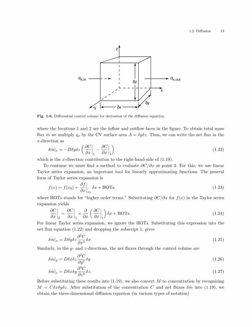
Fig. 1.6. Differential control volume for derivation of the diffusion equation.
where the locations 1 and 2 are the inflow and outflow faces in the figure. To obtain total mass
flux m we multiply qx by the CV surface area A = δyδz. Thus, we can write the net flux in the
x-direction as
δm|x = −Dδyδz
(
∂C
∂x
∣
∣
∣
∣
1− ∂C
∂x
∣
∣
∣
∣
2
)
(1.22)
which is the x-direction contribution to the right-hand-side of (1.19).
To continue we must find a method to evaluate ∂C/∂x at point 2. For this, we use linear
Taylor series expansion, an important tool for linearly approximating functions. The general
form of Taylor series expansion is
f(x) = f(x0) +∂f
∂x
∣
∣
∣
∣
x0
δx + HOTs, (1.23)
where HOTs stands for “higher order terms.” Substituting ∂C/∂x for f(x) in the Taylor series
expansion yields
∂C
∂x
∣
∣
∣
∣
2=
∂C
∂x
∣
∣
∣
∣
1+
∂
∂x
(
∂C
∂x
∣
∣
∣
∣
1
)
δx + HOTs. (1.24)
For linear Taylor series expansion, we ignore the HOTs. Substituting this expression into the
net flux equation (1.22) and dropping the subscript 1, gives
δm|x = Dδyδz∂2C
∂x2δx. (1.25)
Similarly, in the y- and z-directions, the net fluxes through the control volume are
δm|y = Dδxδz∂2C
∂y2δy (1.26)
δm|z = Dδxδy∂2C
∂z2δz. (1.27)
Before substituting these results into (1.19), we also convert M to concentration by recognizing
M = Cδxδyδz. After substitution of the concentration C and net fluxes δm into (1.19), we
obtain the three-dimensional diffusion equation (in various types of notation)

14 1. Concepts, Definitions, and the Diffusion Equation
∂C
∂t= D
(
∂2C
∂x2+
∂2C
∂y2+
∂2C
∂z2
)
= D∇2C
= D∂C
∂x2i
, (1.28)
which is a fundamental equation in environmental fluid mechanics. For the last line in (1.28),
we have used the Einsteinian notation of repeated indices as a short-hand for the ∇2 operator.
1.2.4 One-dimensional diffusion equation
In the one-dimensional case, concentration gradients in the y- and z-direction are zero, and we
have the one-dimensional diffusion equation
∂C
∂t= D
∂2C
∂x2. (1.29)
We pause here to consider (1.29) and to point out a few key observations. First, (1.29) is first-
order in time. Thus, we must supply and impose one initial condition for its solution, and its
solutions will be unsteady, or transient, meaning they will vary with time. To solve for the
steady, time-invariant solution of (1.29), we must set ∂C/∂t = 0 and we no longer require an
initial condition; the steady form of (1.29) is the well-known Laplace equation. Second, (1.29) is
second-order in space. Thus, we must impose two boundary conditions, and its solution will vary
in space. Third, the form of (1.29) is exactly the same as the heat equation, where D is replaced
by the heat transfer coefficient κ. This observation agrees well with our intuition since we know
that heat conducts (diffuses) away from hot sources toward cold regions (just as concentration
diffuses from high concentration toward low concentration). This observation is also useful since
many solutions to the heat equation are already known.
1.3 Similarity solution to the one-dimensional diffusion equation
Because (1.28) is of such fundamental importance in environmental fluid mechanics, we demon-
strate here one of its solutions for the one-dimensional case in detail. There are multiple methods
that can be used to solve (1.28), but we will follow the methodology of Fischer et al. (1979) and
choose the so-called similarity method in order to demonstrate the usefulness of dimensional
analysis as presented in Section 1.1.3.
Consider the one-dimensional problem of a narrow, infinite pipe (radius a) as depicted in
Figure 1.7. A mass of tracer M is injected uniformly across the cross-section of area A = πa2 at
the point x = 0 at time t = 0. The initial width of the tracer is infinitesimally small. We seek
a solution for the spread of the tracer in the x-direction over time due to molecular diffusion
alone.
As this is a one-dimensional (∂C/∂y = 0 and ∂C/∂z = 0) unsteady diffusion problem, (1.29)
is the governing equation, and we require two boundary conditions and an initial condition. As
boundary conditions, we impose that the concentration at ±∞ remain zero

1.3 Similarity solution to the one-dimensional diffusion equation 15
A M
-x x
Fig. 1.7. Definitions sketch for one-dimensional pure diffusion in an infinite pipe.
Table 1.2. Dimensional variables for one-dimensional pipe diffusion.
Variable Dimensions
dependent variable C M/L3
independent variables M/A M/L2
D L2/T
x L
t T
C(±∞, t) = 0 (1.30)
because it is not possible for any of the tracer molecules to wander all the way out to infinity—
by definition, infinity is not reachable. The initial condition is that the dye tracer is injected
uniformly across the cross-section over an infinitesimally small width in the x-direction. To
specify such an initial condition, we use the Dirac delta function
C(x, 0) = (M/A)δ(x) (1.31)
where δ(x) is zero everywhere accept at x = 0, where it is infinite, but the integral of the delta
function from −∞ to ∞ is 1. Thus, the total injected mass is given by
M =
∫
VC(x, t)dV (1.32)
=
∫ ∞
−∞
∫ a
0(M/A)δ(x)2πrdrdx. (1.33)
= M QED. (1.34)
To use dimensional analysis, we must consider all the parameters that control the solution.
Table 1.2 summarizes the dependent and independent variables for our problem. There are m = 5
parameters and n = 3 dimensions; thus, we can form two dimensionless groups
π1 =C
M/(A√
Dt)(1.35)
π2 =x√Dt
(1.36)
From dimensional analysis we have that π1 = f(π2), which implies for the solution of C
C =M
A√
Dtf
(
x√Dt
)
(1.37)

16 1. Concepts, Definitions, and the Diffusion Equation
where f is a yet-unknown function with argument π2. (1.37) is called a similarity solution because
C has the same shape in x at all times t (see also Example Box 1.3). Now we need to find f in
order to know what that shape is. Before we find the solution formally, compare (1.37) with the
actual solution given by (1.59). Through this comparison, we see that dimensional analysis can
go a long way toward finding solutions to physical problems.
The function f can be found in two primary ways. First, experiments can be conducted and
then a smooth curve can be fit to the data using the coordinates π1 and π2. Second, (1.37) can
be used as the solution to a differential equation and f solved for analytically. This is what we
will do here. The power of a similarity solution is that it turns a partial differential equation
(PDE) into an ordinary differential equation (ODE), which is the goal of any solution method
for PDEs.
The similarity solution (1.37) is really just a coordinate transformation. We will call our new
similarity variable η = x/√
Dt. To substitute (1.37) into the diffusion equation, we will need the
two derivatives
∂η
∂t= − η
2t(1.38)
∂η
∂x=
1√Dt
. (1.39)
We first use the chain rule to compute ∂C/∂t as follows
∂C
∂t=
∂
∂t
[
M
A√
Dtf(η)
]
=∂
∂t
[
M
A√
Dt
]
f(η) +M
A√
Dt
∂f
∂η
∂η
∂t
=M
A√
Dt
(
−1
2
)
1
tf(η) +
M
A√
Dt
∂f
∂η
(
− η
2t
)
= − M
2At√
Dt
(
f + η∂f
∂η
)
. (1.40)
Similarly, we use the chain rule to compute ∂2C/∂x2 as follows
∂2C
∂x2=
∂
∂x
[
∂
∂x
(
M
A√
Dtf(η)
)]
=∂
∂x
[
M
A√
Dt
∂η
∂x
∂f
∂η
]
=M
ADt√
Dt
∂2f
∂η2. (1.41)
Upon substituting these two results into the diffusion equation, we obtain the ordinary differen-
tial equation in η
d2f
dη2+
1
2
(
f + ηdf
dη
)
= 0. (1.42)
To solve (1.42), we should also convert the boundary and initial conditions to two new
constraints on f . Substituting η into the boundary conditions gives
1.3 Similarity solution to the one-dimensional diffusion equation 17
C(±∞, t) = 0
M
A√
Dtf
(
x√Dt
)∣
∣
∣
∣
x=±∞= 0
f(±∞) = 0. (1.43)
We convert the initial condition in a similar manner. Substituting η leads to
C(x, 0) =M
Aδx
M
A√
Dtf
(
x√Dt
)∣
∣
∣
∣
t=0
=M
Aδx
Rearranging the terms yields
f
(
x√Dt
)∣
∣
∣
∣
t=0
=√
Dtδx∣
∣
∣
t=0(1.44)
The left hand side will give +∞ if x > 0 and −∞ if x < 0. The right hand side gives zero
because the√
Dt term is always zero at t = 0. Then, the initial condition reduces to
f(±∞) = 0. (1.45)
Thus, the three conditions on the original partial differential equation (two boundary condi-
tions and an initial condition) have been reduced to two boundary conditions on the ordinary
differential equation in f , given by either (1.43) or (1.45).
Another constraint is required to fix the value of M and is taken from the conservation of
mass, given by (1.32). Substituting dx = dη√
Dt into (1.32) and simplifying, we obtain∫ ∞
−∞f(η)dη = 1. (1.46)
Solving (1.42) requires a couple of integrations. First, we rearrange the equation using the
identity
d(fη)
dη= f + η
df
dη, (1.47)
which gives us
d
dη
[
df
dη+
1
2fη
]
= 0. (1.48)
Integrating once leaves us with
df
dη+
1
2fη = C0. (1.49)
It can be shown that choosing C0 = 0 is required to satisfy the boundary conditions (see
Appendix A for more details). For now, we will select C0 = 0 and then verify that the solution
we obtain does indeed obey the boundary condition f(±∞) = 0.
With C0 = 0 we have a homogeneous ordinary differential equation whose solution can readily
be found. Moving the second term to the right hand side we have
df
dη= −1
2fη. (1.50)

18 1. Concepts, Definitions, and the Diffusion Equation
The solution is found by collecting the f - and η-terms on separate sides of the equation
df
f= −1
2ηdη. (1.51)
Integrating both sides gives
ln(f) = −1
2
η2
2+ C1 (1.52)
which after taking the exponential of both sides gives
f = C1 exp
(
−η2
4
)
. (1.53)
To find C1 we must use the remaining constraint given in (1.46). This is necessary since we
introduce a parameter M and we would like that the integral under the concentration curve give
us back the total mass. This auxiliary condition in f gives (recall (1.46))∫ ∞
−∞C1 exp
(
−η2
4
)
dη = 1. (1.54)
To solve this integral, we should use integral tables; therefore, we have to make one more change
of variables to remove the 1/4 from the exponential. Thus, we introduce ζ such that
ζ2 =1
22η2 (1.55)
2dζ = dη. (1.56)
Substituting this coordinate transformation and solving for C1 leaves
C1 =1
2∫∞−∞ exp(−ζ2)dζ
. (1.57)
After looking up the integral in a table, we obtain C1 = 1/(2√
π). Thus,
f(η) =1
2√
πexp
(
η2
4
)
. (1.58)
Replacing f in our similarity solution (1.37) gives
C(x, t) =M
A√
4πDtexp
(
− x2
4Dt
)
(1.59)
which is a classic result in environmental fluid mechanics, and an equation that will be used
thoroughly throughout this text. Generalizing to three dimensions, Fischer et al. (1979) give the
the solution
C(x, y, z, t) =M
4πt√
4πDxDyDztexp
(
− x2
4Dxt− y2
4Dyt− z2
4Dzt
)
(1.60)
which they derive using the separation of variables method.
1.3 Similarity solution to the one-dimensional diffusion equation 19
Example Box 1.2:Maximum concentrations.
For the three-dimensional instantaneous point-source solution given in (1.60), find an expressionfor the maximum concentration. Where is the max-imum concentration located?
The classical approach for finding maxima of func-tions is to look for zero-points in the derivative ofthe function. For many concentration distributions,it is easier to take a qualitative look at the functionalform of the equation. The instantaneous point-sourcesolution has the form
C(x, t) = C1(t) exp(−|f(x, t)|).C1(t) is an amplification factor independent of space.The exponential function has a negative argument,which means it is maximum when the argument iszero. Hence, the maximum concentration is
Cmax(t) = C1(t).
Applying this result to (1.60) gives
Cmax(t) =M
4πt√
4πDxDyDzt.
The maximum concentration occurs at the pointwhere the exponential is zero. In this casex(Cmax) = (0, 0, 0).
We can apply this same analysis to other concen-tration distributions as well. For example, considerthe error function concentration distribution
C(x, t) =C0
2
(
1 − erf
(
x√4Dt
))
.
The error function ranges over [−1, 1] as its argu-ment ranges from [−∞,∞]. The maximum concen-tration occurs when erf(·) = -1, and gives,
Cmax(t) = C0.
Cmax occurs when the argument of the error functionis −∞. At t = 0, the maximum concentration occursfor all points x < 0, and for t > 0, the maximumconcentration occurs only at x = −∞.
−4 −2 0 2 40
0.2
0.4
0.6
0.8
1Point source solution
η = x / (4Dt)1/2
C A
(4π
D t)
1/2 /
M
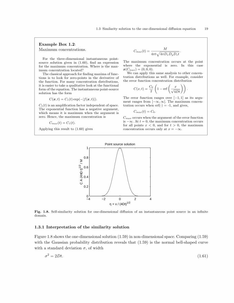
Fig. 1.8. Self-similarity solution for one-dimensional diffusion of an instantaneous point source in an infinitedomain.
1.3.1 Interpretation of the similarity solution
Figure 1.8 shows the one-dimensional solution (1.59) in non-dimensional space. Comparing (1.59)
with the Gaussian probability distribution reveals that (1.59) is the normal bell-shaped curve
with a standard deviation σ, of width
σ2 = 2Dt. (1.61)

20 1. Concepts, Definitions, and the Diffusion Equation
The concept of self similarity is now also evident: the concentration profile shape is always
Gaussian. By plotting in non-dimensional space, the profiles also collapse into a single profile;
thus, profiles for all times t > 0 are given by the result in the figure.
The Gaussian distribution can also be used to predict how much tracer is within a certain
region. Looking at Figure 1.8 it appears that most of the tracer is between -2 and 2. Gaussian
probability tables, available in any statistics book, can help make this observation more quanti-
tative. Within ±σ, 64.2% of the tracer is found and between ±2σ, 95.4% of the tracer is found.
As an engineering rule-of-thumb, we will say that a diffusing tracer is distributed over a region
of width 4σ, that is, ±2σ in Figure 1.8.
Example Box 1.3:Profile shape and self similarity.
For the one-dimensional, instantaneous point-source solution, show that the ratio C/Cmax can bewritten as a function of the single parameter α de-fined such that x = ασ. How might this be used toestimate the diffusion coefficient from concentrationprofile data?
From the previous example, we know that Cmax =M/
√4πDt, and we can re-write (1.59) as
C(x, t)
Cmax(t)= exp
(
− x2
4Dt
)
.
We now substitute σ =√
2Dt and x = ασ to obtain
C
Cmax= exp
(
−α2/2)
.
Here, α is a parameter that specifies the point tocalculate C based on the number of standard devia-tions the point is away from the center of mass. Thisillustrates very clearly the notion of self similarity:regardless of the time t, the amount of mass M , orthe value of D, the ratio C/Cmax is always the samevalue at the same position ασ.
This relationship is very helpful for calculatingdiffusion coefficients. Often, we do not know thevalue of M . We can, however, always normalize aconcentration profile measured at a given time t byCmax(t). Then we pick a value of α, say 1.0. We knowfrom the relationship above that C/Cmax = 0.61 atx = σ. Next, find the locations where C/Cmax =0.61 in the experimental profile and use them to mea-sure σ. We then use the relationship σ =
√2Dt and
the value of t to estimate D.
1.4 Application: Diffusion in a lake
With a solid background now in diffusion, consider the following example adapted from Nepf
(1995).
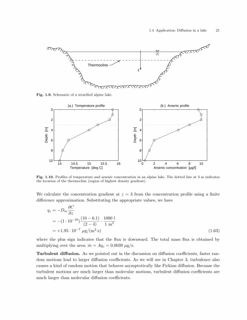
As shown in Figures 1.9 and 1.10, a small alpine lake is mildly stratified, with a thermocline
(region of steepest density gradient) at 3 m depth, and is contaminated by arsenic. Determine the
magnitude and direction of the diffusive flux of arsenic through the thermocline (cross-sectional
area at the thermocline is A = 2 · 104 m2) and discuss the nature of the arsenic source. The
molecular diffusion coefficient is Dm = 1 · 10−10 m2/s.
Molecular diffusion. To compute the molecular diffusive flux through the thermocline, we use
the one-dimensional version of Fick’s law, given above in (1.16)
qz = −Dm∂C
∂z. (1.62)
1.4 Application: Diffusion in a lake 21
Thermoclinez
Fig. 1.9. Schematic of a stratified alpine lake.
14 14.5 15 15.5 16
0
2
4
6
8
10
(a.) Temperature profile
Temperature [deg C]
Dep
th [
m]
0 2 4 6 8 10
0
2
4
6
8
10
(b.) Arsenic profile
Arsenic concentration [µg/l]
Dep
th [
m]
Fig. 1.10. Profiles of temperature and arsenic concentration in an alpine lake. The dotted line at 3 m indicatesthe location of the thermocline (region of highest density gradient).
We calculate the concentration gradient at z = 3 from the concentration profile using a finite
difference approximation. Substituting the appropriate values, we have
qz = −Dm∂C
∂z
= −(1 · 10−10)(10 − 6.1)
(2 − 4)· 1000 l
1 m3
= +1.95 · 10−7 µg/(m2·s) (1.63)
where the plus sign indicates that the flux is downward. The total mass flux is obtained by
multiplying over the area: m = Aqz = 0.0039 µg/s.
Turbulent diffusion. As we pointed out in the discussion on diffusion coefficients, faster ran-
dom motions lead to larger diffusion coefficients. As we will see in Chapter 3, turbulence also
causes a kind of random motion that behaves asymptotically like Fickian diffusion. Because the
turbulent motions are much larger than molecular motions, turbulent diffusion coefficients are
much larger than molecular diffusion coefficients.

22 1. Concepts, Definitions, and the Diffusion Equation
Sources of turbulence at the thermocline of a small lake can include surface inflows, wind
stirring, boundary mixing, convection currents, and others. Based on studies in this lake, a
turbulent diffusion coefficient can be taken as Dt = 1.5 · 10−6 m2/s. Since turbulent diffusion
obeys the same Fickian flux law, then the turbulent diffusive flux qz,t can be related to the
molecular diffusive flux qz,t = qz by the equation
qz,t = qz,mDt
Dm(1.64)
= +2.93 · 10−3 µg/(m2·s). (1.65)
Hence, we see that turbulent diffusive transport is much greater than molecular diffusion. As
a warning, however, if the concentration gradients are very high and the turbulence is low,
molecular diffusion can become surprisingly significant!
Implications. Here, we have shown that the concentration gradient results in a net diffusive
flux of arsenic into the hypolimnion (region below the thermocline). Assuming no other transport
processes are at work, we can conclude that the arsenic source is at the surface. If the diffusive
transport continues, the hypolimnion concentrations will increase. The next chapter considers
how the situation might change if we include another type of transport: advection.
Summary
This chapter introduced the subject of environmental fluid mechanics and focused on the impor-
tant transport process of diffusion. Fick’s law was derived to represent the mass flux (transport)
due to diffusion, and Fick’s law was used to derive the diffusion equation, which is used to pre-
dict the time-evolution of a concentration field in space due to diffusive transport. A similarity
method was used through the aid of dimensional analysis to find a one-dimensional solution
to the diffusion equation for an instantaneous point source. As illustrated through an example,
diffusive transport results when concentration gradients exist and plays an important role in
predicting the concentrations of contaminants as they move through the environment.
Exercises
1.1 Newspaper research. Find an example of a news article that deals with fate or transport
of chemicals in a situation that demonstrates concepts from Environmental Fluid Mechanics.
You my chose a newspaper or web article, and the event should have occurred in the last
20 years. Attach a copy of the article and write a short paragraph describing it’s relationship to
environmental fluid mechanics.
1.2 Definitions. Write a short, qualitative definition of the following terms:
Concentration. Partial differential equation.
Mass fraction. Standard deviation.
Density. Chemical fate.

Exercises 23
Diffusion. Chemical transport.
Brownian motion. Transport equation.
Instantaneous point source. Fick’s law.
Similarity method.
1.3 Concentrations in water. A student adds 1.00 mg of pure Rhodamine WT (a common
fluorescent tracer used in field experiments) to 1.000 l of water at 20C. Assuming the solution
is dilute so that we can neglect the equation of state of the solution, compute the concentration
of the Rhodamine WT mixture in the units of mg/l, mg/kg, ppm, and ppb.
1.4 Concentrations in air. Air consists of 21% oxygen gas (O2). For air with a density of
1.4 kg/m3, compute the concentration of oxygen in the units of mg/l, mg/kg, mol/l, and ppm.
1.5 Fick’s law. Assume a linear concentration profile between two fixed points as depicted in
the following figure:
C
C0 C(x)
C1
Lx0
and given by the equation
C = bx + C0 (1.66)
where b = (C1 − C0)/L. Assuming the diffusion coefficient is D, find:
• The diffusive flux per unit area for any point between x = [0, L].
• The total mass flux over an area A between x = [0, L].
1.6 Mass fluxes. A one-dimensional concentration profile near a fixed-concentration sewage dis-
charge is
C(x) = C0
(
1 − erf
(
x√4Dt
))
(1.67)
where C0 is the initial concentration near the source, erf is the error function, t is the time since
the start of release, x is the distance downstream, and D is the diffusion coefficient. Compute
the net mass flux vector qx at x = 10 m and t = 6 hours. Use D = 1 · 10−3 m2/s.
1.7 Diffusive flux in a side channel. A small fish pond located near a river bank downstream
of a mine is connected to the main river through a small channel for water intake (refer to the
figure below). Assume the water levels between the river and the pond are the same so that the
velocity in the channel is zero. The arsenic level in the river is on average 1 ppm during the
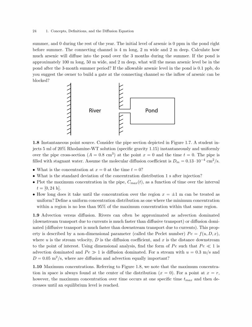
24 1. Concepts, Definitions, and the Diffusion Equation
summer, and 0 during the rest of the year. The initial level of arsenic is 0 ppm in the pond right
before summer. The connecting channel is 4 m long, 2 m wide and 2 m deep. Calculate how
much arsenic will diffuse into the pond over the 3 months during the summer. If the pond is
approximately 100 m long, 50 m wide, and 2 m deep, what will the mean arsenic level be in the
pond after the 3-month summer period? If the allowable arsenic level in the pond is 0.1 ppb, do
you suggest the owner to build a gate at the connecting channel so the inflow of arsenic can be
blocked?
River Pond
1.8 Instantaneous point source. Consider the pipe section depicted in Figure 1.7. A student in-
jects 5 ml of 20% Rhodamine-WT solution (specific gravity 1.15) instantaneously and uniformly
over the pipe cross-section (A = 0.8 cm3) at the point x = 0 and the time t = 0. The pipe is
filled with stagnant water. Assume the molecular diffusion coefficient is Dm = 0.13 ·10−4 cm2/s.
• What is the concentration at x = 0 at the time t = 0?
• What is the standard deviation of the concentration distribution 1 s after injection?
• Plot the maximum concentration in the pipe, Cmax(t), as a function of time over the interval
t = [0, 24 h].
• How long does it take until the concentration over the region x = ±1 m can be treated as
uniform? Define a uniform concentration distribution as one where the minimum concentration
within a region is no less than 95% of the maximum concentration within that same region.
1.9 Advection versus diffusion. Rivers can often be approximated as advection dominated
(downstream transport due to currents is much faster than diffusive transport) or diffusion domi-
nated (diffusive transport is much faster than downstream transport due to currents). This prop-
erty is described by a non-dimensional parameter (called the Peclet number) Pe = f(u, D, x),
where u is the stream velocity, D is the diffusion coefficient, and x is the distance downstream
to the point of interest. Using dimensional analysis, find the form of Pe such that Pe 1 is
advection dominated and Pe 1 is diffusion dominated. For a stream with u = 0.3 m/s and
D = 0.05 m2/s, where are diffusion and advection equally important?
1.10 Maximum concentrations. Referring to Figure 1.8, we note that the maximum concentra-
tion in space is always found at the center of the distribution (x = 0). For a point at x = r,
however, the maximum concentration over time occurs at one specific time tmax and then de-
creases until an equilibrium level is reached.

Exercises 25
• Using the one-dimensional point source solution, find an equation for the time tmax at which
the maximum concentration occurs for an arbitrary point x = r.
• Write a program (MATLAB is preferred, but not required) that solves the one-dimensional
point source solution at x = r with r, D, M , and A as user inputs. Plot the concentration as
a function of time at the location r = 2 with the remaining three inputs set as 1.0. Plot an
adequate time period that the maximum concentration is clearly identifiable. (Please mail me
your program).
• Calculate tmax for the case plotted in the previous step (r = 2, D = M = A = 1) and compare
your value to the figure from your Matlab program.
1.11 Diffusion in a river. The Rhein river can be approximated as having a uniform depth
(h = 5 m), width (B = 300 m) and mean flow velocity (u = 0.7 m/s). Under these conditions,
100 kg of tracer is injected as a point source (the injection is evenly distributed transversely over
the cross-section). The cloud is expected to diffuse laterally as a one-dimensional point source
in a moving coordinate system, moving at the mean stream velocity. The river has an enhanced
mixing coefficient of D = 10 m2/s. How long does it take for the center of mass of the cloud to
reach a point x = 15000 m downstream? What is the maximum concentration that passes the
point x? How wide is the cloud (take the cloud width as 4σ) when it passes this point?
1.12 Measuring diffusion coefficients 1. A chemist is trying to calculate the diffusion coefficient
for a new chemical. In his experiments, he measured the concentration as a function of time
at a point 5 cm away from a virtual point source diffusing in three dimensions. Select a set of
coordinates such that, when plotting the data in Table 1.3, D is the slope of a best-fit line through
the data. Based on this coordinate transformation, what is more important to measure precisely,
concentration or time? What recommendation would you give to this scientist to improve the
accuracy of his estimate for the diffusion coefficient?
1.13 Measuring diffusion coefficients 2.1 As part of a water quality study, you have been asked
to assess the diffusion of a new fluorescent dye. To accomplish this, you do a dye study in a
laboratory tank (depth h = 40 cm). You release the dye at a depth of 20 cm (spread evenly over
the area of the tank) and monitor its development over time. Vertical profiles of dye concentration
in the tank are shown in Figure 1.11; the x-axis represents the reading on your fluorometer and
the y-axis represents the depth.
• Estimate the molecular diffusion coefficient of the dye, Dm, based on the evolution of the dye
cloud.
• Predict at what time the vertical distribution of the dye will be affected by the boundaries of
the tank.
1.14 Radiative heaters. A student heats his apartment (surface area Ar = 32 m2 and ceiling
height h = 3 m) with a radiative heater. The heater has a total surface area of Ah = 0.8 m2;
the thickness of the heater wall separating the heater fluid from the outside air is δx = 3 mm
1 This problem is adapted from Nepf (1995).
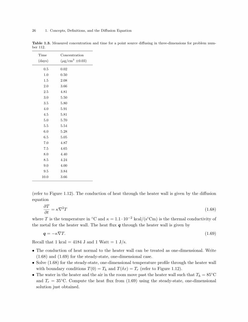
26 1. Concepts, Definitions, and the Diffusion Equation
Table 1.3. Measured concentration and time for a point source diffusing in three-dimensions for problem num-ber 112.
Time Concentration
(days) (µg/cm3 ±0.03)
0.5 0.02
1.0 0.50
1.5 2.08
2.0 3.66
2.5 4.81
3.0 5.50
3.5 5.80
4.0 5.91
4.5 5.81
5.0 5.70
5.5 5.54
6.0 5.28
6.5 5.05
7.0 4.87
7.5 4.65
8.0 4.40
8.5 4.24
9.0 4.00
9.5 3.84
10.0 3.66
(refer to Figure 1.12). The conduction of heat through the heater wall is given by the diffusion
equation
∂T
∂t= κ∇2T (1.68)
where T is the temperature in C and κ = 1.1 · 10−2 kcal/(sCm) is the thermal conductivity of
the metal for the heater wall. The heat flux q through the heater wall is given by
q = −κ∇T. (1.69)
Recall that 1 kcal = 4184 J and 1 Watt = 1 J/s.
• The conduction of heat normal to the heater wall can be treated as one-dimensional. Write
(1.68) and (1.69) for the steady-state, one-dimensional case.
• Solve (1.68) for the steady-state, one-dimensional temperature profile through the heater wall
with boundary conditions T (0) = Th and T (δx) = Tr (refer to Figure 1.12).
• The water in the heater and the air in the room move past the heater wall such that Th = 85C
and Tr = 35C. Compute the heat flux from (1.69) using the steady-state, one-dimensional
solution just obtained.

Exercises 27
0 0.02 0.04 0.06 0.08
0
5
10
15
20
25
30
35
40
Concentration [g/cm3]
Dep
th [
cm]
Profile after 14 days
0 0.01 0.02 0.03 0.04 0.05
0
5
10
15
20
25
30
35
40
Profile after 35 days
Concentration [g/cm3]
Dep
th [
cm]
Fig. 1.11. Concentration profiles of fluorescent dye for two different measurement times. Refer to problemnumber 1.13.
• How many 300 Watt lamps are required to equal the heat output of the heater assuming 100%
efficiency?
• Assume the specific heat capacity of the air is cv = 0.172 kcal/(kg·K) and the density is
ρa = 1.4 kg/m3. How much heat is required to raise the temperature of the apartment by
5C?
• Given the heat output of the heater and the heat needed to heat the room, how might you
explain that the student is able to keep the heater turned on all the time?

28 1. Concepts, Definitions, and the Diffusion Equation
Heaterfluid
Roomair
Th Ta
δ x
Steel heater wall
Fig. 1.12. Definitions sketch for one-dimensional thermal conduction for the heater wall in problem number 1.14.
2. Advective Diffusion Equation
In nature, transport occurs in fluids through the combination of advection and diffusion. The
previous chapter introduced diffusion and derived solutions to predict diffusive transport in
stagnant ambient conditions. This chapter incorporates advection into our diffusion equation
(deriving the advective diffusion equation) and presents various methods to solve the resulting
partial differential equation for different geometries and contaminant conditions.
2.1 Derivation of the advective diffusion equation
Before we derive the advective diffusion equation, we look at a heuristic description of the effect
of advection. To conceptualize advection, consider our pipe problem from the previous chapter.
Without pipe flow, the injected tracer spreads equally in both directions, describing a Gaussian
distribution over time. If we open a valve and allow water to flow in the pipe, we expect the
center of mass of the tracer cloud to move with the mean flow velocity in the pipe. If we move
our frame of reference with that mean velocity and assume the inviscid case, then we expect the
solution to look the same as before. This new reference frame is
η = x − (x0 + ut) (2.1)
where η is the moving reference frame spatial coordinate, x0 is the injection point of the tracer,
u is the mean flow velocity, and ut is the distance traveled by the center of mass of the cloud
in time t. If we substitute η for x in our solution for a point source in stagnant conditions we
obtain
C(x, t) =M
A√
4πDtexp
(
−(x − (x0 + ut))2
4Dt
)
. (2.2)
To test whether this solution is correct, we need to derive a general equation for advective
diffusion and compare its solution to this one.
2.1.1 The governing equation
The derivation of the advective diffusion equation relies on the principle of superposition: ad-
vection and diffusion can be added together if they are linearly independent. How do we know
if advection and diffusion are independent processes? The only way that they can be dependent
is if one process feeds back on the other. From the previous chapter, diffusion was shown to be
a random process due to molecular motion. Due to diffusion, each molecule in time δt will move
Copyright c© 2004 by Scott A. Socolofsky and Gerhard H. Jirka. All rights reserved.
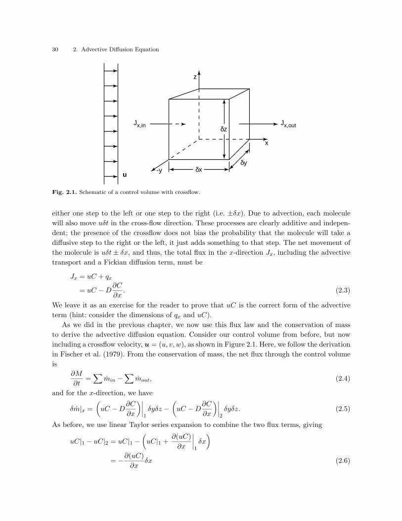
30 2. Advective Diffusion Equation
Jx,in Jx,out
x
-y
z
δxδy
δz
u
Fig. 2.1. Schematic of a control volume with crossflow.
either one step to the left or one step to the right (i.e. ±δx). Due to advection, each molecule
will also move uδt in the cross-flow direction. These processes are clearly additive and indepen-
dent; the presence of the crossflow does not bias the probability that the molecule will take a
diffusive step to the right or the left, it just adds something to that step. The net movement of
the molecule is uδt ± δx, and thus, the total flux in the x-direction Jx, including the advective
transport and a Fickian diffusion term, must be
Jx = uC + qx
= uC − D∂C
∂x. (2.3)
We leave it as an exercise for the reader to prove that uC is the correct form of the advective
term (hint: consider the dimensions of qx and uC).
As we did in the previous chapter, we now use this flux law and the conservation of mass
to derive the advective diffusion equation. Consider our control volume from before, but now
including a crossflow velocity, u = (u, v, w), as shown in Figure 2.1. Here, we follow the derivation
in Fischer et al. (1979). From the conservation of mass, the net flux through the control volume
is
∂M
∂t=∑
min −∑
mout, (2.4)
and for the x-direction, we have
δm|x =
(
uC − D∂C
∂x
)∣
∣
∣
∣
1δyδz −
(
uC − D∂C
∂x
)∣
∣
∣
∣
2δyδz. (2.5)
As before, we use linear Taylor series expansion to combine the two flux terms, giving
uC|1 − uC|2 = uC|1 −(
uC|1 +∂(uC)
∂x
∣
∣
∣
∣
1δx
)
= −∂(uC)
∂xδx (2.6)

2.1 Derivation of the advective diffusion equation 31
and
− D∂C
∂x
∣
∣
∣
∣
1+ D
∂C
∂x
∣
∣
∣
∣
2= −D
∂C
∂x
∣
∣
∣
∣
1+
(
D∂C
∂x
∣
∣
∣
∣
1+
∂
∂x
(
D∂C
∂x
)∣
∣
∣
∣
1δx
)
= D∂2C
∂x2δx. (2.7)
Thus, for the x-direction
δm|x = −∂(uC)
∂xδxδyδz + D
∂2C
∂x2δxδyδz. (2.8)
The y- and z-directions are similar, but with v and w for the velocity components, giving
δm|y = −∂(vC)
∂yδyδxδz + D
∂2C
∂y2δyδxδz (2.9)
δm|z = −∂(wC)
∂zδzδxδy + D
∂2C
∂z2δzδxδy. (2.10)
Substituting these results into (2.4) and recalling that M = Cδxδyδz, we obtain
∂C
∂t+ ∇ · (uC) = D∇2C (2.11)
or in Einsteinian notation
∂C
∂t+
∂uiC
∂xi= D
∂2C
∂x2i
, (2.12)
which is the desired advective diffusion (AD) equation. We will use this equation extensively in
the remainder of this text.
Note that these equations implicitly assume that D is constant. When considering a variable
D, the right-hand-side of (2.12) has the form
∂
∂xi
(
Dij∂C
∂xj
)
. (2.13)
2.1.2 Point-source solution
To check whether our initial suggestion (2.2) for a solution to (2.12) was correct, we substitute
the coordinate transformation for the moving reference frame into the one-dimensional version
of (2.12). In the one-dimensional case, u = (u, 0, 0), and there are no concentration gradients in
the y- or z-directions, leaving us with
∂C
∂t+
∂(uC)
∂x= D
∂2C
∂x2. (2.14)
Our coordinate transformation for the moving system is
η = x − (x0 + ut) (2.15)
τ = t, (2.16)
and this can be substituted into (2.14) using the chain rule as follows

32 2. Advective Diffusion Equation
0 1 2 3 4 5 6 7 8 9 100
0.5
1
1.5Solution of the advective−diffusion equation
Position
Con
cent
ratio
n
t1
t2 t
3
Cmax
Fig. 2.2. Schematic solution of the advective diffusion equation in one dimension. The dotted line plots themaximum concentration as the cloud moves downstream.
∂C
∂τ
∂τ
∂t+
∂C
∂η
∂η
∂t+ u
(
∂C
∂η
∂η
∂x+
∂C
∂τ
∂τ
∂x
)
=
D
(
∂
∂η
∂η
∂x+
∂
∂τ
∂τ
∂x
)(
∂C
∂η
∂η
∂x+
∂C
∂τ
∂τ
∂x
)
(2.17)
which reduces to
∂C
∂τ= D
∂2C
∂η2. (2.18)
This is just the one-dimensional diffusion equation (1.29) in the coordinates η and τ with solution
for an instantaneous point source of
C(η, τ) =M
A√
4πDτexp
(
− η2
4Dτ
)
. (2.19)
Converting the solution back to x and t coordinates (by substituting (2.15) and (2.16)), we
obtain (2.2); thus, our intuitive guess for the superposition solution was correct. Figure 2.2
shows the schematic behavior of this solution for three different times, t1, t2, and t3.
2.1.3 Incompressible fluid
For an incompressible fluid, (2.12) can be simplified by using the conservation of mass equation
for the ambient fluid. In an incompressible fluid, the density is a constant ρ0 everywhere, and
the conservation of mass equation reduces to the continuity equation
∇ · u = 0 (2.20)
(see, for example Batchelor (1967)). If we expand the advective term in (2.12), we can write
∇ · (uC) = (∇ · u)C + u · ∇C. (2.21)
by virtue of the continuity equation (2.20) we can take the term (∇·u)C = 0; thus, the advective
diffusion equation for an incompressible fluid is

2.1 Derivation of the advective diffusion equation 33
∂C
∂t+ ui
∂C
∂xi= D
∂2C
∂x2i
. (2.22)
This is the form of the advective diffusion equation that we will use the most in this class.
2.1.4 Rules of thumb
We pause here to make some observations regarding the AD equation and its solutions.
First, the solution in Figure 2.2 shows an example where the diffusive and advective transport
are about equally important. If the crossflow were stronger (larger u), the cloud would have less
time to spread out and would be narrower at each ti. Conversely, if the diffusion were faster
(larger D), the cloud would spread out more between the different ti and the profiles would
overlap. Thus, we see that diffusion versus advection dominance is a function of t, D, and u,
and we express this property through the non-dimensional Peclet number
Pe =D
u2t, (2.23)
or for a given downstream location L = ut,
Pe =D
uL. (2.24)
For Pe 1, diffusion is dominant and the cloud spreads out faster than it moves downstream;
for Pe 1, advection is dominant and the cloud moves downstream faster than it spreads out.
It is important to note that the Peclet number is dependent on our zone of interest: for “large”
times or distances, the Peclet number is small and advection dominates.
Second, the maximum concentration decreases in the downstream direction due to diffusion.
Figure 2.2 also plots the maximum concentration of the cloud as it moves downstream. This is
obtained when the exponential term in (2.2) is 1.0. For the one-dimensional case, the maximum
concentration decreases as
Cmax(t) ∝ 1√t. (2.25)
In the two- and three-dimensional cases, the relationship is
Cmax(t) ∝ 1
tand (2.26)
Cmax(t) ∝ 1
t√
t, (2.27)
respectively.
Third, the diffusive and advective scales can be used to simplify the equations and make ap-
proximations. One of the most common questions in engineering is: when does a given equation
or approximation apply? In contaminant transport, this question is usually answered by com-
paring characteristic advection and diffusion length and time scales to the length and time scales
in the problem. For advection (subscript a) and for diffusion (subscript d), the characteristic
scales are

34 2. Advective Diffusion Equation
La = ut ; ta =L
u(2.28)
Ld =√
Dt ; td =L2
D. (2.29)
These scales can be used as a rule-of-thumb estimate for when or where certain events take
place. For instance, for a point source released in the middle of a region of width L and bounded
at ±L/2 by impermiable boundaries, the time required before the cloud can be considered well-
mixed over the region by diffusion is tm,d = L2/(8D). The coefficient value 8 is derived by
requiring that the concentration at ±L/2 be at least 97% of the maximum concentration Cmax.
These characteristic scales (easily derivable through dimensional analysis) should be memorized
and used extensively to get a rough solution to transport problems.
2.2 Solutions to the advective diffusion equation
In the previous chapter we presented a detailed solution for an instantaneous point source in a
stagnant ambient. In nature, initial and boundary conditions can be much different from that
idealized case, and this section presents a few techniques to deal with other general cases. Just as
advection and diffusion are additive, we will also show that superpostion can be used to build up
solutions to complex geometries or initial conditions from a base set of a few general solutions.
The solutions in this section parallel a similar section in Fischer et al. (1979). Appendix B
presents analytical solutions for other initial and boundary conditions, primarily obtained by
extending the techniques discussed in this section. Taken together, these solutions can be applied
to a wide range of problems.
2.2.1 Initial spatial concentration distribution
A good example of the power of superposition is the solution for an initial spatial concentration
distribution. Since advection can always be included by changing the frame of reference, we will
consider the one-dimensional stagnant case. Thus, the governing equation is
∂C
∂t= D
∂2C
∂x2. (2.30)
We will consider the homogeneous initial distribution, given by
C(x, t0) =
C0 if x ≤ 0
0 if x > 0(2.31)
where t0 = 0 and C0 is the uniform initial concentration, as depicted in Figure 2.3. At a point
x = ξ < 0 there is an infinitesimal mass dM = C0Adξ, where A is the cross-sectional area δyδz.
For t > 0, the concentration at any point x is due to the diffusion of mass from all the differential
elements dM . The contribution dC for a single element dM is just the solution of (2.30) for an
instantaneous point source
dC(x, t) =dM
A√
4πDtexp
(
−(x − ξ)2
4Dt
)
, (2.32)

2.2 Solutions to the advective diffusion equation 35
C
x
dM = C0Ad
C0
d x
ξ
ξFig. 2.3. Schematic of an instantaneous initial concentration distribution showing the differential element dM atthe point −ξ.
and by virtue of superposition, we can sum up all the contributions dM to obtain
C(x, t) =
∫ 0
−∞
C0dξ√4πDt
exp
(
−(x − ξ)2
4Dt
)
(2.33)
which is the superposition solution to our problem. To compute the integral, we must, as usual,
make a change of variables. The new variable ζ is defined as follows
ζ =x − ξ√
4Dt(2.34)
dζ = − dξ√4Dt
. (2.35)
Substituting ζ into the integral solution gives
C(x, t) =C0√
π
∫ x/√
4Dt
∞− exp(−ζ2)dζ. (2.36)
Note that to obtain the upper bound on the integral we set ξ = 0 in the definition for ζ given
in (2.34). Rearranging the integral gives
C(x, t) =C0√
π
∫ ∞
x/√
4Dtexp(−ζ2)dζ (2.37)
=C0√
π
[
∫ ∞
0exp(−ζ2)dζ −
∫ x/√
4Dt
0exp(−ζ2)dζ
]
. (2.38)
The first of the two integrals can be solved analytically—from a table of integrals, its solution
is√
π/2. The second integral is the so called error function, defined as
erf(ϕ) =2√π
∫ ϕ
0exp(−ζ2)dζ. (2.39)
Solutions to the error function are generally found in tables or as built-in functions in a spread-
sheet or computer programming language. Hence, our solution can be written as
C(x, t) =C0
2
(
1 − erf
(
x√4Dt
))
. (2.40)
Figure 2.4 plots this solution for C0 = 1 and for increasing times t.
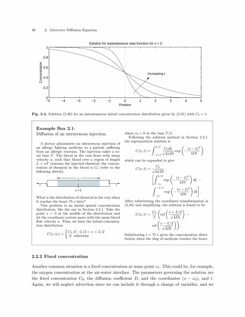
36 2. Advective Diffusion Equation
−5 −4 −3 −2 −1 0 1 2 3 4 50
0.2
0.4
0.6
0.8
1Solution for instantaneous step function for x < 0
Position
Con
cent
ratio
n
Increasing t
Fig. 2.4. Solution (2.40) for an instantaneous initial concentration distribution given by (2.31) with C0 = 1.
Example Box 2.1:Diffusion of an intravenous injection.
A doctor administers an intravenous injection ofan allergy fighting medicine to a patient sufferingfrom an allergic reaction. The injection takes a to-tal time T . The blood in the vein flows with meanvelocity u, such that blood over a region of lengthL = uT contains the injected chemical; the concen-tration of chemical in the blood is C0 (refer to thefollowing sketch).
L
-x x
x = 0
What is the distribution of chemical in the vein whenit reaches the heart 75 s later?
This problem is an initial spatial concentrationdistribution, like the one in Section 2.2.1. Take thepoint x = 0 at the middle of the distribution andlet the coordinate system move with the mean bloodflow velocity u. Thus, we have the initial concentra-tion distribution
C(x, t0) =
C0 if −L/2 < x < L/20 otherwise
where t0 = 0 at the time T/2.Following the solution method in Section 2.2.1,
the superposition solution is
C(x, t) =
∫ L/2
−L/2
C0dξ√4πDt
exp
(
− (x − ξ)2
4Dt
)
which can be expanded to give
C(x, t) =C0√4πDt
·[∫ L/2
−∞
exp
(
− (x − ξ)2
4Dt
)
dξ −∫
−L/2
−∞
exp
(
− (x − ξ)2
4Dt
)
dξ
]
.
After substituting the coordinate transformation in(2.34) and simplifying, the solution is found to be
C(x, t) =C0
2
(
erf
(
x + L/2√4Dt
)
−
erf
(
x − L/2√4Dt
))
.
Substituting t = 75 s gives the concentration distri-bution when the slug of medicine reaches the heart.
2.2.2 Fixed concentration
Another common situation is a fixed concentration at some point x1. This could be, for example,
the oxygen concentration at the air-water interface. The parameters governing the solution are
the fixed concentration C0, the diffusion coefficient D, and the coordinates (x − x0), and t.
Again, we will neglect advection since we can include it through a change of variables, and we
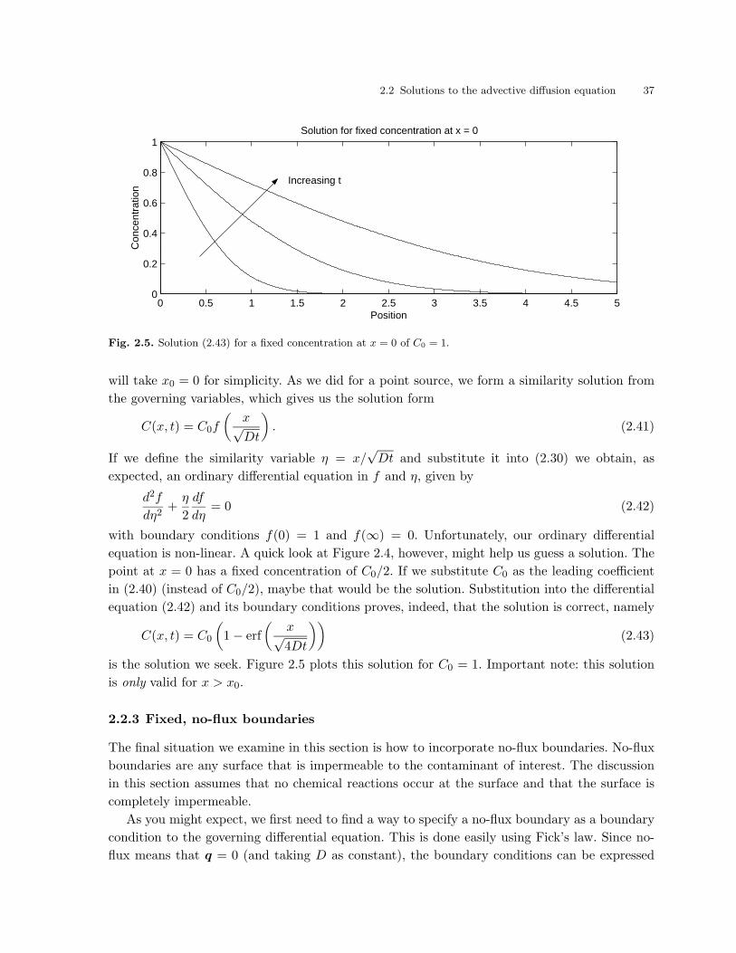
2.2 Solutions to the advective diffusion equation 37
0 0.5 1 1.5 2 2.5 3 3.5 4 4.5 50
0.2
0.4
0.6
0.8
1Solution for fixed concentration at x = 0
Position
Con
cent
ratio
n
Increasing t
Fig. 2.5. Solution (2.43) for a fixed concentration at x = 0 of C0 = 1.
will take x0 = 0 for simplicity. As we did for a point source, we form a similarity solution from
the governing variables, which gives us the solution form
C(x, t) = C0f
(
x√Dt
)
. (2.41)
If we define the similarity variable η = x/√
Dt and substitute it into (2.30) we obtain, as
expected, an ordinary differential equation in f and η, given by
d2f
dη2+
η
2
df
dη= 0 (2.42)
with boundary conditions f(0) = 1 and f(∞) = 0. Unfortunately, our ordinary differential
equation is non-linear. A quick look at Figure 2.4, however, might help us guess a solution. The
point at x = 0 has a fixed concentration of C0/2. If we substitute C0 as the leading coefficient
in (2.40) (instead of C0/2), maybe that would be the solution. Substitution into the differential
equation (2.42) and its boundary conditions proves, indeed, that the solution is correct, namely
C(x, t) = C0
(
1 − erf
(
x√4Dt
))
(2.43)
is the solution we seek. Figure 2.5 plots this solution for C0 = 1. Important note: this solution
is only valid for x > x0.
2.2.3 Fixed, no-flux boundaries
The final situation we examine in this section is how to incorporate no-flux boundaries. No-flux
boundaries are any surface that is impermeable to the contaminant of interest. The discussion
in this section assumes that no chemical reactions occur at the surface and that the surface is
completely impermeable.
As you might expect, we first need to find a way to specify a no-flux boundary as a boundary
condition to the governing differential equation. This is done easily using Fick’s law. Since no-
flux means that q = 0 (and taking D as constant), the boundary conditions can be expressed

38 2. Advective Diffusion Equation
Example Box 2.2:Dissolving sugar in coffee.
On a cold winter’s day you pour a cup of coffee andadd 2 g of sugar evenly distributed over the bottomof the coffee cup. The diameter of the cup is 5 cm;its height is 7 cm. If you do not stir the coffee, whendoes the concentration boundary layer first reach thetop of the cup and when does all of the sugar dis-solve? How would these answers change if you stirthe coffee?
The concentration of sugar is fixed at the satu-ration concentration at the bottom of the cup andis initially zero everywhere else. These are the sameconditions as for the fixed concentration solution;thus, the sugar distribution at height z above thebottom of the cup is
C(z, t) = C0
(
1 − erf
(
z√4Dt
))
.
The characteristic height of the concentrationboundary layer is proportional to σ =
√2Dt. As-
sume the concentration boundary layer first reachesthe top of the cup when 2σ = h = 7 cm. Solving fortime gives
tmix,bl =h2
8D.
For an order-of-magnitude estimate, take D ∼10−9 m2/s, giving
tmix,bl ≈ 6 · 105 s.
To determine how long it takes for the sugar todissolve, we must compute the mass flux of sugar atz = 0. We already computed the derivative of theerror function in Example Box 1.1. The mass flux ofsugar at z = 0 is then
m(0, t) =ADCsat√
πDt
where A is the cross-sectional area of the cup. The to-tal amount of dissolved sugar Md is the time-integralof the mass flux
Md =
∫ t
0
ADCsat√πDτ
dτ
Integrating and solving for time gives
td =M2
d π
4A2DC2sat
where td is the time it takes for the mass Md todissolve. This expression is only valid for t < tmix,bl;for times beyond tmix,bl, we must account for theboundary at the top of the cup. Assuming Csat =0.58 g/cm3, the time needed to dissolve all the sugaris
td = 5 · 104 s.
By stirring, we effectively increase the value of D.Since D is in the denominator of each of these timeestimates, we shorten the time for the sugar to dis-solve and mix throughout the cup.
as
q|Sb· n = 0
(
∂C
∂x,∂C
∂y,∂C
∂z
)∣
∣
∣
∣
Sb
· n = 0 (2.44)
where Sb is the function describing the boundary surface (i.e. Sb = f(x, y)) and n is the unit vec-
tor normal to the no-flux boundary. In the one-dimensional case, the no-flux boundary condition
reduces to
∂C
∂x
∣
∣
∣
∣
xb
= 0, (2.45)
where xb is the boundary location. This property is very helpful in interpreting concentration
measurements to determine whether a boundary, for instance, the lake bottom, is impermeable
or not.
To find a solution to a bounded problem, consider an instantaneous point source injected
at x0 with a no-flux boundary a distance L to the right as shown in Figure 2.6. Our standard
solution allows mass to diffuse beyond the no-flux boundary (as indicated by the dashed line in

2.3 Application: Diffusion in a Lake 39
Boundary
Imagesource
Realsource
Superpositionsolution
2L
C
x
x0
Fig. 2.6. Schematic of a no-flux boundary with real instantaneous point source to the left and an imaginarysource to the right. The dotted lines indicate the individual contributions from the two sources; the solid lineindicates the superposition solution.
the figure). To replace this lost mass, an image source (imaginary source) is placed to the right
of the boundary, such that it leaks the same amount of mass back to left of the boundary as
our standard solution leaked to the right. Superposing (adding) these two solutions gives us the
desired no-flux behavior at the wall. The image source is placed L to the right of the boundary,
and the solution is
C(x, t) =M
A√
4πDt
(
exp
(
−(x − x0)2
4Dt
)
+ exp
(
−(x − xi)2
4Dt
))
(2.46)
where xi = x0 + 2L. Naturally, the solution given here is only valid to the left of the boundary.
To the right of the boundary, the concentration is everywhere zero. Compute the concentration
gradient ∂C/∂x at x = 0 to prove to yourself that the no-flux boundary condition is satisfied.
The method of images becomes more complicated when multiple boundaries are concerned.
This is because the mass diffusing from the image source on the right eventually will penetrate a
boundary on the left and need its own image source. In general, when there are two boundaries,
an infinite number of image sources is required. In practice, the solution usually converges after
only a few image sources have been included (Fischer et al. 1979). For the case of an instantaneous
point source at the origin with boundaries at ±L, Fischer et al. (1979) give the image source
solution
C(x, t) =M
A√
4πDt
∞∑
n=−∞exp
(
−(x + 2nL)2
4Dt
)
. (2.47)
Obviously, the number of image sources required for the solution to converge depends on the
time scale over which the solution is to be valid. These techniques will become more clear in the
following examples and remaining chapters.
2.3 Application: Diffusion in a Lake
We return here to the application of arsenic contamination in a small lake presented in Chapter 1
(adapted from Nepf (1995)). After further investigation, it is determined that a freshwater spring
flows into the bottom of the lake with a flow rate of 10 l/s.
40 2. Advective Diffusion Equation
Example Box 2.3:Boundaries in a coffee cup.
In the previous example box we said that we haveto account for the free surface boundary when theconcentration boundary layer reaches the top of thecoffee cup. Describe the image source needed to ac-count for the free surface and state the image-sourcesolution for the concentration distribution.
We can ignore the boundaries at the sides of thecup because sugar is evenly distributed on the bot-tom of the cup. This even distribution results in∂C/∂x = ∂C/∂y = 0, which results in no net dif-fusive flux toward the cup walls.
To account for the free surface, though, we mustadd an image source with a fixed concentration ofCsat somewhere above the cup. Taking z = 0 at thebottom of the cup, the image source must be placedat z = 2h, where h is the depth of coffee in the cup.
Taking care that C(z,∞) → Csat, the superposi-tion solution for the sugar concentration distributioncan be found to be
C(z, t) = Csat
(
1 + erf
(
2h√4Dt
)
−
erf
(
z√4Dt
)
− erf
(
2h − z√4Dt
))
.
Advection. Advection is due to the flow of spring water through the lake. Assuming the spring
is not buoyant, it will spread out over the bottom of the lake and rise with a uniform vertical
flux velocity (recall that z is positive downward, so the flow is in the minus z-direction)
va = −Q/A
= −5 · 10−7 m/s. (2.48)
The concentration of arsenic at the thermocline is 8 µg/l, which results in an advective flux of
arsenic
qa = Cva
= −4 · 10−3 µg/(m2s). (2.49)
Thus, advection caused by the spring results in a vertical advective flux of arsenic through the
thermocline.
Discussion. Taking the turbulent and advective fluxes of arsenic together, the net vertical flux
of arsenic through the thermocline is
Jz = −4.00 · 10−3 + 2.93 · 10−3
= −1.10 · 10−3 µg/(m2s) (2.50)
where the minus sign indicates the net flux is upward. Thus, although the net diffusive flux is
downward, the advection caused by the stream results in the net flux at the thermocline being
upward. We can conclude that the arsenic source is likely at the bottom of the lake. The water
above the thermocline will continue to increase in concentration until the diffusive flux at the
thermocline becomes large enough to balance the advective flux through the lake, at which time
the system will reach a steady state.
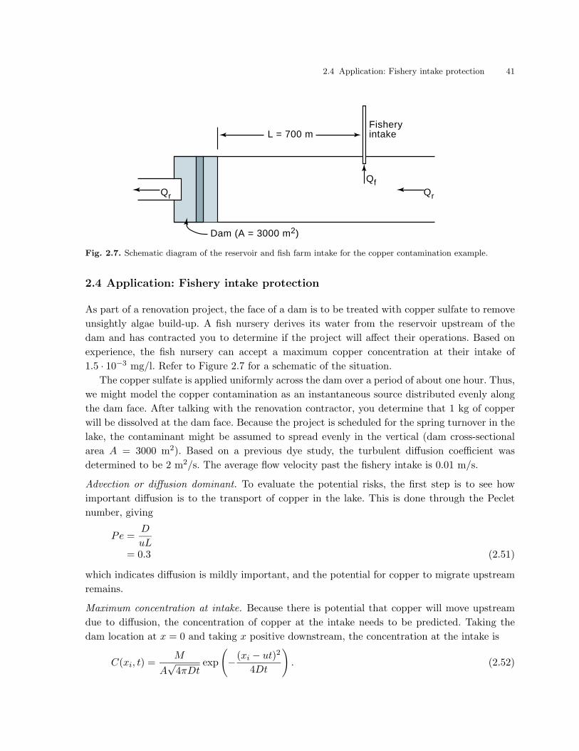
2.4 Application: Fishery intake protection 41
Fisheryintake
Dam (A = 3000 m2)
L = 700 m
Qr
QfQr
Fig. 2.7. Schematic diagram of the reservoir and fish farm intake for the copper contamination example.
2.4 Application: Fishery intake protection
As part of a renovation project, the face of a dam is to be treated with copper sulfate to remove
unsightly algae build-up. A fish nursery derives its water from the reservoir upstream of the
dam and has contracted you to determine if the project will affect their operations. Based on
experience, the fish nursery can accept a maximum copper concentration at their intake of
1.5 · 10−3 mg/l. Refer to Figure 2.7 for a schematic of the situation.
The copper sulfate is applied uniformly across the dam over a period of about one hour. Thus,
we might model the copper contamination as an instantaneous source distributed evenly along
the dam face. After talking with the renovation contractor, you determine that 1 kg of copper
will be dissolved at the dam face. Because the project is scheduled for the spring turnover in the
lake, the contaminant might be assumed to spread evenly in the vertical (dam cross-sectional
area A = 3000 m2). Based on a previous dye study, the turbulent diffusion coefficient was
determined to be 2 m2/s. The average flow velocity past the fishery intake is 0.01 m/s.
Advection or diffusion dominant. To evaluate the potential risks, the first step is to see how
important diffusion is to the transport of copper in the lake. This is done through the Peclet
number, giving
Pe =D
uL= 0.3 (2.51)
which indicates diffusion is mildly important, and the potential for copper to migrate upstream
remains.
Maximum concentration at intake. Because there is potential that copper will move upstream
due to diffusion, the concentration of copper at the intake needs to be predicted. Taking the
dam location at x = 0 and taking x positive downstream, the concentration at the intake is
C(xi, t) =M
A√
4πDtexp
(
−(xi − ut)2
4Dt
)
. (2.52)
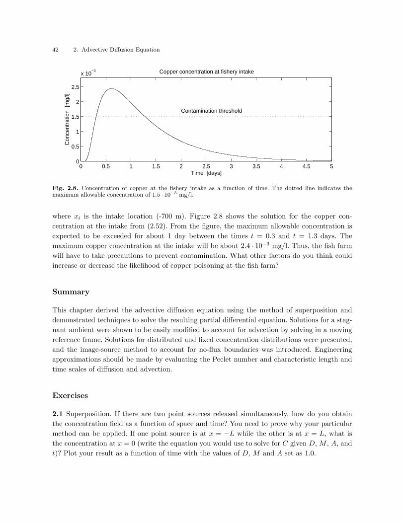
42 2. Advective Diffusion Equation
0 0.5 1 1.5 2 2.5 3 3.5 4 4.5 50
0.5
1
1.5
2
2.5
x 10−3 Copper concentration at fishery intake
Time [days]
Con
cent
ratio
n [m
g/l]
Contamination threshold
Fig. 2.8. Concentration of copper at the fishery intake as a function of time. The dotted line indicates themaximum allowable concentration of 1.5 · 10−3 mg/l.
where xi is the intake location (-700 m). Figure 2.8 shows the solution for the copper con-
centration at the intake from (2.52). From the figure, the maximum allowable concentration is
expected to be exceeded for about 1 day between the times t = 0.3 and t = 1.3 days. The
maximum copper concentration at the intake will be about 2.4 · 10−3 mg/l. Thus, the fish farm
will have to take precautions to prevent contamination. What other factors do you think could
increase or decrease the likelihood of copper poisoning at the fish farm?
Summary
This chapter derived the advective diffusion equation using the method of superposition and
demonstrated techniques to solve the resulting partial differential equation. Solutions for a stag-
nant ambient were shown to be easily modified to account for advection by solving in a moving
reference frame. Solutions for distributed and fixed concentration distributions were presented,
and the image-source method to account for no-flux boundaries was introduced. Engineering
approximations should be made by evaluating the Peclet number and characteristic length and
time scales of diffusion and advection.
Exercises
2.1 Superposition. If there are two point sources released simultaneously, how do you obtain
the concentration field as a function of space and time? You need to prove why your particular
method can be applied. If one point source is at x = −L while the other is at x = L, what is
the concentration at x = 0 (write the equation you would use to solve for C given D, M , A, and
t)? Plot your result as a function of time with the values of D, M and A set as 1.0.

Exercises 43
2.2 Integral evaluation. Define an appropriate coordinate transformation and show that
I =1√π
∫ 4Dt+x2/√
Dt
−∞2x
√Dt exp
−(
x2
√Dt
+ 4Dt
)2
dx (2.53)
can also be written as
I =Dt
2
(
erf
(
x2
√Dt
+ 4Dt
)
− 1
)
(2.54)
2.3 Non-dimensionalization. Non-dimensionalize the three-dimensional diffusion equation and
find the important parameter(s) in the equation. Use a single length scale for all three dimensions.
Discuss your parameter(s) in a brief paragraph.
2.4 Peclet number. A river with cross section A = 20 m2 has a flow rate of Q = 1 m3/s. The
effective mixing coefficient is D = 1 m2/s. For what distance downstream is diffusion dominant?
Where does advection become dominant? What is the length of stream where diffusion and
advection have about equal influence?
2.5 Advection in a stream. To estimate the mixing characteristics of a small stream, a scientist
injects 5 g of dye instantaneously and uniformly over the river cross section (A = 5 m2) at the
point x = 0. A measurement station is located 1 km downstream and records a river flow rate
of Q = 0.5 m3/s. In order to design the experiment, the scientist assumed that D = 0.1 m2/s.
Use this value to answer the following equations.
• The fluorometer used to measure the dye downstream at the measuring station has a detection
limit of 0.1 µg/l. When does the measuring station first detect the dye cloud?
• When does the maximum dye concentration pass the measuring station, and what is this
maximum concentration?
• After the maximum concentration passes the measuring station, the measured concentration
decreases again. When is the measuring station no longer able to detect the dye?
• Why is the elapsed time between first detection and the maximum concentration different
from the elapsed time between the last detection and the maximum concentration?
2.6 Fixed concentration. A beaker in a laboratory contains a solution with dissolved methane
gas (CH4). The concentration of methane in the atmosphere Ca is negligible; the concentration
of methane in the uniformly-mixed portion of the beaker is Cw. The methane in the beaker
dissolves out of the water and into the air, resulting in a fixed concentration at the water surface
of Cws = 0. Assume this process is limited by diffusion of methane through the water.
• Write an expression for the vertical concentration distribution of methane in the beaker.
Assume the bottom boundary does not affect the profile (concentration at the bottom is Cw)
and that methane is uniformly distributed in the horizontal (use the one-dimensional solution).
• Use the expression found above to find an expression for the flux of methane into the atmo-
sphere through the water surface.
2.7 Concentration profiles. Figure 2.9 shows four concentration profiles measured very carefully
at the bottom of four different lakes. For each profile, state whether the lake bottom is a no-flux
or flux boundary and describe where you think the source is located and why.

44 2. Advective Diffusion Equation
z
Lake CC
z
Lake DC
z
Lake AC
z
Lake BC
Fig. 2.9. Bottom concentration profiles for the four lakes in problem number 2.4.
2.8 Double point sources. To demonstrate the image-source method, a professor creates two
instantaneous point sources of dye (three dimensional) a distance L apart and measures the
concentration of dye at the point halfway between the two sources. Estimate the radius of the
cloud for each point source by r = 2σ.
• Write an expression for the time t when the two sources first touch.
• Write an expression for the concentration distribution along the line connecting the two point
sources.
• Differentiate this solution to show that the net flux through the measurement point along the
axis of the two sources is zero.
2.9 The time-scale for a point source injected mid-way between two impermeable boundaries
to become uniformly mixed across the section is given by the rule-of-thumb
tm =L2
8D(2.55)
where L is the distance between the two boundaries and D is the diffusion coefficient. Referring
to the sketch below, consider a line of dye released instantaneously along the centerline of a
shallow river so that the problem can be treated as one-dimensional.
• Write a program applying the superposition method to calculate the relative concentration
(relative to the centerline concentration of the river C(x = 0, t)) at the river bank x = L/2
as a function of time, that is, find the ratio C(L/2, t)/C(0, t). The width of the river is L and
the diffusion coefficient of the dye is D (please email me your final program).
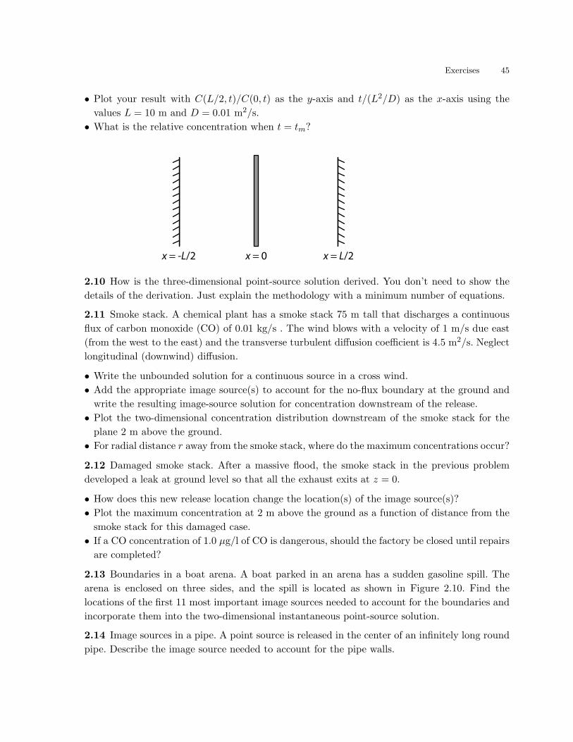
Exercises 45
• Plot your result with C(L/2, t)/C(0, t) as the y-axis and t/(L2/D) as the x-axis using the
values L = 10 m and D = 0.01 m2/s.
• What is the relative concentration when t = tm?
x = -L/2 x = L/2x = 0
2.10 How is the three-dimensional point-source solution derived. You don’t need to show the
details of the derivation. Just explain the methodology with a minimum number of equations.
2.11 Smoke stack. A chemical plant has a smoke stack 75 m tall that discharges a continuous
flux of carbon monoxide (CO) of 0.01 kg/s . The wind blows with a velocity of 1 m/s due east
(from the west to the east) and the transverse turbulent diffusion coefficient is 4.5 m2/s. Neglect
longitudinal (downwind) diffusion.
• Write the unbounded solution for a continuous source in a cross wind.
• Add the appropriate image source(s) to account for the no-flux boundary at the ground and
write the resulting image-source solution for concentration downstream of the release.
• Plot the two-dimensional concentration distribution downstream of the smoke stack for the
plane 2 m above the ground.
• For radial distance r away from the smoke stack, where do the maximum concentrations occur?
2.12 Damaged smoke stack. After a massive flood, the smoke stack in the previous problem
developed a leak at ground level so that all the exhaust exits at z = 0.
• How does this new release location change the location(s) of the image source(s)?
• Plot the maximum concentration at 2 m above the ground as a function of distance from the
smoke stack for this damaged case.
• If a CO concentration of 1.0 µg/l of CO is dangerous, should the factory be closed until repairs
are completed?
2.13 Boundaries in a boat arena. A boat parked in an arena has a sudden gasoline spill. The
arena is enclosed on three sides, and the spill is located as shown in Figure 2.10. Find the
locations of the first 11 most important image sources needed to account for the boundaries and
incorporate them into the two-dimensional instantaneous point-source solution.
2.14 Image sources in a pipe. A point source is released in the center of an infinitely long round
pipe. Describe the image source needed to account for the pipe walls.
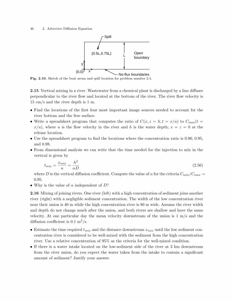
46 2. Advective Diffusion Equation
Open boundary
x
y
(0,0)
L(0.5L,0.75L)
Spill
No-flux boundariesFig. 2.10. Sketch of the boat arena and spill location for problem number 2.4.
2.15 Vertical mixing in a river. Wastewater from a chemical plant is discharged by a line diffuser
perpendicular to the river flow and located at the bottom of the river. The river flow velocity is
15 cm/s and the river depth is 1 m.
• Find the locations of the first four most important image sources needed to account for the
river bottom and the free surface.
• Write a spreadsheet program that computes the ratio of C(x, z = h, t = x/u) to Cmax(t =
x/u), where u is the flow velocity in the river and h is the water depth; x = z = 0 at the
release location.
• Use the spreadsheet program to find the locations where the concentration ratio is 0.90, 0.95,
and 0.98.
• From dimensional analysis we can write that the time needed for the injection to mix in the
vertical is given by
tmix =xmix
u=
h2
αD(2.56)
where D is the vertical diffusion coefficient. Compute the value of α for the criteria Cmin/Cmax =
0.95.
• Why is the value of α independent of D?
2.16 Mixing of joining rivers. One river (left) with a high concentration of sediment joins another
river (right) with a negligible sediment concentration. The width of the low concentration river
near their union is 40 m while the high concentration river is 80 m wide. Assume the river width
and depth do not change much after the union, and both rivers are shallow and have the same
velocity. At one particular day the mean velocity downstream of the union is 1 m/s and the
diffusion coefficient is 0.1 m2/s.
• Estimate the time required tmix and the distance downstream xmix until the low sediment con-
centration river is considered to be well-mixed with the sediment from the high concentration
river. Use a relative concentration of 95% as the criteria for the well-mixed condition.
• If there is a water intake located on the low-sediment side of the river at 3 km downstream
from the river union, do you expect the water taken from the intake to contain a significant
amount of sediment? Justify your answer.

Exercises
47
Table 2.1: Table of solutions to the diffusion equation
Schematic and Solution
Instantaneous point source, infinite domain
C
x
C(x,t = 0) =
x0
δ (x-x0)MA
8
C
x
Cmax
2σ1
4σ2
C(x, t) =M
A√
4πDtexp
[
− (x − x0)2
4Dt
]
Cmax(t) =M
A√
4πDt
qx(x, t) =M(x − x0)
2At√
4πDtexp
[
− (x − x0)2
4Dt
]
Let σ =√
2Dt and(2σ)2 = 8Dt.For x0 = 0:C(±σ, t) = 0.61Cmax(t)
Let σ =√
2Dt and(4σ)2 = 32Dt.For x0 = 0:C(±2σ, t) = 0.14Cmax(t)
Instantaneous distributed source, infinite domain
C
x
C(x,t = 0) =
x0
C
x
2σ1
C0, x < x0
0, x > x0
C02
4σ2
C(x, t) =C0
2
[
1 − erf
[
(x − x0)√4Dt
]]
Cmax(t) = C0
qx(x, t) =C0
√D√
4πtexp
[
− (x − x0)2
4Dt
]
Let σ =√
2Dt and(2σ)2 = 8Dt.For x0 = 0:C(+σ, t) = 0.16C0
C(−σ, t) = 0.84C0
Let σ =√
2Dt and(4σ)2 = 32Dt.For x0 = 0:C(+2σ, t) = 0.02C0
C(−2σ, t) = 0.98C0

48
2.
Advectiv
eD
iffusio
nE
quatio
nTable 2.1: (continued)
Schematic Solution
Fixed concentration, semi-infinite domain
C
x
C(x=x0,t ) = C0
x0
C
x
σ
C0
C0
2σ
C(x > x0, t) = C0
[
1 − erf
[
(x − x0)√4Dt
]]
Cmax(t) = C0
qx(x > x0, t) =2C0
√D√
4πtexp
[
− (x − x0)2
4Dt
]
Let σ =√
2Dt andσ2 = 2Dt.For x0 = 0:C(+σ, t) = 0.32C0
C(−σ, t) = Undefined
Let σ =√
2Dt and(2σ)2 = 8Dt.For x0 = 0:C(+2σ, t) = 0.05C0
C(−2σ, t) = Undefined
Instantaneous point source, bounded domain
C
x
C(x,t = 0) =
x0
δ (x-x0)MA
8
C
x
Cmax
dCdx
= 0xb
2Lb
C(x, t) =M
A√
4πDt
∞∑
n=−∞
exp
[
− (x − x0 + 2nLb)2
4Dt
]
Cmax(t) =M
A√
4πDt
∞∑
n=−∞
exp
[
− (2nLb)2
4Dt
]
qx(x, t) =M
2At√
4πDt
∞∑
n=−∞
(x − x0 + 2nLb) exp
[
− (x − x0 + 2nLb)2
4Dt
]
Using the image-sourcemethod, the first imageon the opposite side ofthe boundary is atx0 ± 2Lb.
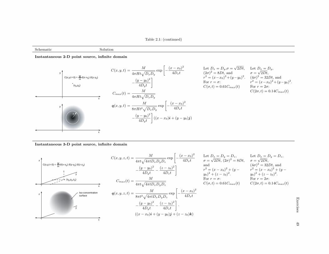
Exercises
49
Table 2.1: (continued)
Schematic Solution
Instantaneous 2-D point source, infinite domain
y
x
C(x,y,t = 0) = δ (x-x0)MH
y
x
δ (y-y0)
(x0,y0)
σ
C(x, y, t) =M
4πHt√
DxDy
exp
[
− (x − x0)2
4Dxt
− (y − y0)2
4Dyt
]
Cmax(t) =M
4πHt√
DxDy
q(x, y, t) =M
8πHt2√
DxDy
exp
[
− (x − x0)2
4Dxt
− (y − y0)2
4Dyt
]
((x − x0)i + (y − y0)j)
Let Dx = Dy,σ =√
2Dt,(2σ)2 = 8Dt, andr2 = (x−x0)
2+(y−y0)2.
For r = σ:C(σ, t) = 0.61Cmax(t)
Let Dx = Dy,σ =
√2Dt,
(4σ)2 = 32Dt, andr2 = (x−x0)
2+(y−y0)2.
For r = 2σ:C(2σ, t) = 0.14Cmax(t)
Instantaneous 3-D point source, infinite domain
z
x
C(x,y,t = 0) = δ (x-x0)MH
z
x
δ (y-y0)
(x0,y0,z0)
δ (z-z0)
Iso-concentrationsurface
y
y
C(x, y, z, t) =M
4πt√
4πtDxDyDz
exp
[
− (x − x0)2
4Dxt
− (y − y0)2
4Dyt− (z − z0)
2
4Dzt
]
Cmax(t) =M
4πt√
4πtDxDyDz
q(x, y, z, t) =M
8πt2√
4πtDxDyDz
exp
[
− (x − x0)2
4Dxt
− (y − y0)2
4Dyt− (z − z0)
2
4Dzt
]
·
((x − x0)i + (y − y0)j + (z − z0)k)
Let Dx = Dy = Dz,σ =
√2Dt, (2σ)2 = 8Dt,
andr2 = (x − x0)
2 + (y −y0)
2 + (z − z0)2.
For r = σ:C(σ, t) = 0.61Cmax(t)
Let Dx = Dy = Dz,σ =
√2Dt,
(4σ)2 = 32Dt, andr2 = (x − x0)
2 + (y −y0)
2 + (z − z0)2.
For r = 2σ:C(2σ, t) = 0.14Cmax(t)

50 2. Advective Diffusion Equation

3. Mixing in Rivers: Turbulent Diffusion
and Dispersion
In previous chapters we considered the processes of advection and molecular diffusion and have
seen some example problems with so called “turbulent diffusion” coefficients, where we use the
same governing equations, but with larger diffusion (mixing) coefficients. In natural rivers, a
host of processes lead to a non-uniform velocity field, which allows mixing to occur much faster
than by molecular diffusion alone. In this chapter, we formally derive the equations for non-
uniform velocity fields to demonstrate their effects on mixing. First, we consider the effect of a
random, turbulent velocity field. Second, we consider the combined effects of diffusion (molecular
or turbulent) with a shear velocity profile to develop equations for dispersion. In each case, the
resulting equations retain their previous form, but the mixing coefficients are orders of magnitude
greater than the molecular diffusion coefficients.
We start by giving a description of turbulence and its effects on the transport of contaminants.
We then derive a new advective diffusion equation for turbulent flow and show why turbulence
can be described by the regular advective diffusion equation derived previously, but using larger
turbulent diffusion coefficients. We then look at the effect of a shear velocity profile on the
transport of contaminants and derive one-dimensional equations for longitudinal dispersion.
This chapter concludes with a common dye study application to compute the effective mixing
coefficients in rivers.
3.1 Turbulence and mixing
In the late 1800’s, Reynolds performed a series of experiments on the transport of dye streaks in
pipe flow. These were the pioneering observations of turbulence, and his analysis is what gives
the Re number its name. It is interesting to realize that the first contribution to turbulence
research was in the area of contaminant transport (the behavior of dye streaks); therefore, we
can assume that turbulence has an important influence on transport. In his paper, Reynolds
(1883) wrote (taken from Acheson (1990)):
The experiments were made on three tubes. They were all about 4 feet 6 inches
[1.37 m] long, and fitted with trumpet mouthpieces, so that water might enter without
disturbance. The water was drawn through the tubes out of a large glass tank, in which
the tubes were immersed, arrangements being made so that a streak or streaks of highly
colored water entered the tubes with the clear water.
The general results were as follows:
Copyright c© 2004 by Scott A. Socolofsky and Gerhard H. Jirka. All rights reserved.

52 3. Mixing in Rivers: Turbulent Diffusion and Dispersion
Fig. 3.1. Sketches from Reynolds (1883) showing laminar flow (top), turbulent flow (middle), and turbulent flowilluminated with an electric spark (bottom). Taken from Acheson (1990).
1. When the velocities were sufficiently low, the streak of colour extended in a beautiful
straight line through the tube.
2. If the water in the tank had not quite settled to rest, at sufficiently low velocities,
the streak would shift about the tube, but there was no appearance of sinuosity.
3. As the velocity was increased by small stages, at some point in the tube, always at
a considerable distance from the trumpet or intake, the color band would all at once
mix up with the surrounding water, and fill the rest of the tube with a mass of colored
water. Any increase in the velocity caused the point of break down to approach the
trumpet, but with no velocities that were tried did it reach this. On viewing the tube
by the light of an electric spark, the mass of color resolved itself into a mass of more
or less distinct curls, showing eddies.
Figure 3.1 shows the schematic drawings of what Reynolds saw, taken from his paper.
The first case he describes, the one with low velocities, is laminar flow: the fluid moves in
parallel layers along nearly perfect lines, and disturbances are damped by viscosity. The only way
that the dye streak can spread laterally in the laminar flow is through the action of molecular
diffusion; thus, it would take a much longer pipe before molecular diffusion could disperse the
dye uniformly across the pipe cross-section (what rule of thumb could we use to determine the
required length of pipe?).
The latter case, at higher velocities, is turbulent flow: the fluid becomes suddenly unstable
and develops into a spectrum of eddies, and these disturbances grow due to instability. The
dye, which more or less follows the fluid passively, is quickly mixed across the cross-section as
the eddies grow and fill the tube with turbulent flow. The observations with an electric spark
indicate that the dye conforms to the shape of the eddies. After some time, however, the eddies
will have grown and broken enough times that the dye will no longer have strong concentration
gradients that outline the eddies: at that point, the dye is well mixed and the mixing is more or
less random (even though it is still controlled by discrete eddies).

3.1 Turbulence and mixing 53
Reynolds summarized his results by showing that these characteristics of the flow were de-
pendent on the non-dimensional number Re = UL/ν, where U is the mean pipe flow velocity, L
the pipe diameter and ν the kinematic viscosity, and that turbulence occurred at higher values
of Re. The main consequence of turbulence is that it enhances momentum and mass transport.
3.1.1 Mathematical descriptions of turbulence
Much research has been conducted in the field of turbulence. The ideas summarized in the
following can be found in much greater detail in the treatises by Lumley & Panofsky (1964),
Pope (2000), and Mathieu & Scott (2000).
In this section we will consider a special kind of turbulence: homogeneous turbulence. The
term homogeneous means that the statistical properties of the flow are steady (unchanging)—the
flow can still be highly irregular. These homogeneous statistical properties are usually described
by properties of the velocity experienced at a point in space in the turbulent flow (this is an
Eulerian description). To understand the Eulerian properties of turbulence, though, it is useful
to first consider a Lagrangian frame of reference and follow a fluid particle.
In a turbulent flow, large eddies form continuously and break down into smaller eddies so
that there is always a spectrum of eddy sizes present in the flow. As a large eddy breaks down
into multiple smaller eddies, very little kinetic energy is lost, and we say that energy is efficiently
transferred through a cascade of eddy sizes. Eventually, the eddies become small enough that
viscosity takes over, and the energy is damped out and converted into heat. This conversion of
kinetic energy to heat at small scales is called dissipation and is designated by
ε =dissipated kinetic energy
time(3.1)
which has the units [L2/T 3]. Since the kinetic energy is efficiently transferred down to these
small scales, the dissipated kinetic energy must equal the total turbulent kinetic energy of the
flow: this means that production and dissipation of kinetic energy in a homogeneous turbulent
flow are balanced.
The length scale of the eddies in which turbulent kinetic energy is converted to heat is called
the Kolmogorov scale LK . How large is LK? We use dimensional analysis to answer this question
and recognize that LK depends on the rate of dissipation (or, equivalently, production) of energy,
ε, and on the viscosity, ν, since friction converts the kinetic energy to heat. Forming a length
scale from these parameters, we have
LK ∝ ν3/4
ε1/4. (3.2)
This is an important scale in turbulence.
Summarizing the Lagrangian perspective, if we follow a fluid particle, it may begin by being
swept into a large eddy, and then will move from eddy to eddy as the eddies break down,
conserving kinetic energy in the cascade. Eventually, the particle finds itself in a small enough
eddy (one of order LK in size), that viscosity dissipates its kinetic energy into heat. This small
eddy is also a part of a larger eddy; hence, all sizes of eddies are present at all times in the flow.

54 3. Mixing in Rivers: Turbulent Diffusion and Dispersion
0 0.5 1 1.5 2 2.5 3
0.16
0.18
0.2
0.22
Sample Laser Doppler Velocimeter (LDV) data
Time [s]
Vel
ocity
[m
/s]
u'(t)
u
Fig. 3.2. Schematic measurement of the turbulent fluctuating velocity at a point showing the average velocity, uand the fluctuating component, u′(t).
Because it is so difficult to follow a fluid particle with a velocity probe (this is what we try
to do with Particle Tracking Velocimetry (PTV)), turbulent velocity measurements are usually
made at a point, and turbulence is described by an Eulerian reference frame. The spectrum of
eddies pass by the velocity probe, transported with the mean flow velocity. Large eddies produce
long-period velocity fluctuations in the velocity measurement, and small eddies produce short-
period velocity fluctuations, and all these scales are present simultaneously in the flow. Figure 3.2
shows an example of a turbulent velocity measurement for one velocity component at a point.
If we consider a short portion of the velocity measurement, the velocities are highly correlated
and appear deterministic. If we compare velocities further apart in the time-series, the velocities
become completely uncorrelated and appear random. The time-scale at which velocities begin
to appear uncorrelated and random is called the integral time scale tI . In the Lagrangian frame,
this is the time it takes a parcel of water to forget its initial velocity. This time scale can also
be written as a characteristic length and velocity, giving the integral scales uI and lI .
Reynolds suggested that at some time longer than tI , the velocity at a point xi could be
decomposed into a mean velocity ui and a fluctuation u′i such that
ui(xi, t) = ui(xi) + u′i(xi, t), (3.3)
and this treatment of the velocity is called Reynolds decomposition. tI is, then, comparable to
the time it takes for ui to become steady (constant).
One other important descriptor of turbulence is the root-mean-square velocity
urms =√
u′u′ (3.4)
which, since kinetic energy is proportional to a velocity squared, is a measure of the turbulent
kinetic energy of the flow (i.e. the mean flow kinetic energy is subtracted out since u′ is just the
fluctuation from the mean).

3.1 Turbulence and mixing 55
3.1.2 The turbulent advective diffusion equation
To derive an advective diffusion equation for turbulence, we substitute the Reynolds decompo-
sition into the normal equation for advective diffusion and analyze the results. Before we can do
that, we need a Reynolds decomposition analogy for the concentration, namely,
C(xi, t) = C(xi) + C ′(xi, t). (3.5)
Since we are only interested in the long-term (long compared to tI) average behavior of a
tracer cloud, after substituting the Reynolds decomposition, we will also take a time average. As
an example, consider the time-average mass flux in the x-direction at our velocity probe, uC:
qx = uC
= (ui + u′i)(C + C ′)
= uiC + uiC ′ + u′iC + u′
iC′ (3.6)
where the over-bar indicates a time average
uC =1
tI
∫ t+tI
tuCdτ. (3.7)
For homogeneous turbulence, the average of the fluctuating velocities must be zero, u′i = C ′ = 0,
and we have
uC = uiC + u′iC
′ (3.8)
where we drop the double over-bar notation since the average of an average is just the average.
Note that we cannot assume that the cross term u′iC
′ is zero.
With these preliminary tools, we are now ready to substitute the Reynolds decomposition
into the governing advective diffusion equation (with molecular diffusion coefficients) as follows
∂C
∂t+
∂uiC
∂xi=
∂
∂xi
(
D∂C
∂xi
)
∂(C + C ′)
∂t+
∂(ui + u′i)(C + C ′)
∂xi=
∂
∂xi
(
D∂(C + C ′)
∂xi
)
. (3.9)
Next, we integrate over the integral time scale tI
1
tI
∫ t+tI
t
∂(C + C ′)
∂τ+
∂(ui + u′i)(C + C ′)
∂xi=
∂
∂xi
(
D∂(C + C ′)
∂xi
)
dτ
∂(C + C ′)
∂t+
∂(uiC + uiC ′ + u′iC + u′
iC′)
∂xi=
∂
∂xi
(
D∂(C + C ′)
∂xi
)
. (3.10)
Finally, we recognize that the terms uiC ′, u′iC and C ′ are zero, and, after moving the u′
iC′-term
to the right hand side, we are left with
∂C
∂t+ ui
∂C
∂xi= −∂u′
iC′
∂xi+
∂
∂xi
(
D∂C
∂xi
)
. (3.11)

56 3. Mixing in Rivers: Turbulent Diffusion and Dispersion
To utilize (3.11), we require a model for the term u′iC
′. Since this term is of the form uC, we
know that it is a mass flux. Since both components of this term are fluctuating, it must be a mass
flux associated with the turbulence. Reynolds describes this turbulent component qualitatively
as a form of rapid mixing; thus, we might make an analogy with molecular diffusion. Taylor
(1921) derived part of this analogy by analytically tracking a cloud of tracer particles in a
turbulent flow and calculating the Lagrangian autocorrelation function. His result shows that,
for times greater than tI , the cloud of tracer particles grows linearly with time. Rutherford
(1994) and Fischer et al. (1979) use this result to justify an analogy with molecular diffusion,
though it is worth pointing out that Taylor did not take the analogy that far. For the diffusion
analogy model, the average turbulent diffusion time scale is ∆t = tI , and the average turbulent
diffusion length scale is ∆x = uItI = lI ; hence, the model is only valid for times greater than
tI . Using a Fick’s law type relationship for turbulent diffusion gives
u′iC
′ = Dt∂C
∂xi(3.12)
with
Dt =(∆x)2
∆t= uI lI . (3.13)
Substituting this model for the average turbulent diffusive transport into (3.11) and dropping
the over-bar notation gives
∂C
∂t+ ui
∂C
∂xi=
∂
∂xi
(
Dt∂C
∂xi
)
+∂
∂xi
(
Dm∂C
∂xi
)
. (3.14)
As we will see in the next section, Dt is usually much greater than the molecular diffusion
coefficient Dm; thus, the final term is typically neglected.
3.1.3 Turbulent diffusion coefficients in rivers
How big are turbulent diffusion coefficients? To answer this question, we need to determine what
the coefficients depend on and use dimensional analysis.
For this purpose, consider a wide river with depth h and width W h. An important
property of three-dimensional turbulence is that the largest eddies are usually limited by the
smallest spatial dimension, in this case, the depth. This means that turbulent properties in a
wide river should be independent of the width, but dependent on the depth. Also, turbulence
is thought to be generated in zones of high shear, which in a river would be at the bed. A
parameter that captures the strength of the shear (and is also proportional to many turbulent
properties) is the shear velocity u∗ defined as
u∗ =
√
τ0
ρ(3.15)
where τ0 is the bed shear and ρ is the fluid density. For uniform open channel flow, the shear
friction is balanced by gravity, and
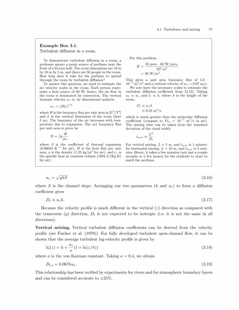
3.1 Turbulence and mixing 57
Example Box 3.1:Turbulent diffusion in a room.
To demonstrate turbulent diffusion in a room, aprofessor sprays a point source of perfume near thefront of a lecture hall. The room dimensions are 10 mby 10 m by 5 m, and there are 50 people in the room.How long does it take for the perfume to spreadthrough the room by turbulent diffusion?
To answer this question, we need to estimate theair velocity scales in the room. Each person repre-sents a heat source of 60 W; hence, the air flow inthe room is dominated by convection. The verticalbuoyant velocity w∗ is, by dimensional analysis,
w∗ = (BL)1/3
where B is the buoyancy flux per unit area in [L2/T3]and L is the vertical dimension of the room (here5 m). The buoyancy of the air increases with tem-perature due to expansion. The net buoyancy fluxper unit area is given by
B = βgH
ρcv
where β is the coefficient of thermal expansion(0.00024 K−1 for air), H is the heat flux per unitarea, ρ is the density (1.25 kg/m3 for air), and cv isthe specific heat at constant volume (1004 J/(Kg·K)for air).
For this problem,
H =50 pers. · 60 W/pers.
102 m2
= 30 W/m2.
This gives a unit area buoyancy flux of 5.6 ·10−5 m2/s3 and a vertical velocity of w∗ = 0.07 m/s.
We now have the necessary scales to estimate theturbulent diffusion coefficient from (3.13). TakinguI ∝ w∗ and lI ∝ h, where h is the height of theroom,
Dt ∝ w∗h
≈ 0.35 m2/s
which is much greater than the molecular diffusioncoefficient (compare to Dm = 10−5 m2/s in air).The mixing time can be taken from the standarddeviation of the cloud width
tmix ≈ L2
Dt.
For vertical mixing, L = 5 m, and tmix is 1 minute;for horizontal mixing, L = 10 m, and tmix is 5 min-utes. Hence, it takes a few minutes (not just a coupleseconds or a few hours) for the students to start tosmell the perfume.
u∗ =√
ghS (3.16)
where S is the channel slope. Arranging our two parameters (h and u∗) to form a diffusion
coefficient gives
Dt ∝ u∗h. (3.17)
Because the velocity profile is much different in the vertical (z) direction as compared with
the transverse (y) direction, Dt is not expected to be isotropic (i.e. it is not the same in all
directions).
Vertical mixing. Vertical turbulent diffusion coefficients can be derived from the velocity
profile (see Fischer et al. (1979)). For fully developed turbulent open-channel flow, it can be
shown that the average turbulent log-velocity profile is given by
ut(z) = u +u∗κ
(1 + ln(z/h)) (3.18)
where κ is the von Karman constant. Taking κ = 0.4, we obtain
Dt,z = 0.067hu∗. (3.19)
This relationship has been verified by experiments for rivers and for atmospheric boundary layers
and can be considered accurate to ±25%.

58 3. Mixing in Rivers: Turbulent Diffusion and Dispersion
Example Box 3.2:Vertical mixing in a river.
A factory waste stream is introduced through alateral diffuser at the bed of a river, as shown in thefollowing sketch.
ασ
L
At what distance downstream can the injection beconsidered as fully mixed in the vertical?
The assumption of “fully mixed” can be definedas the condition where concentration variations overthe cross-section are below a threshold criteria. Sincethe vertical domain has two boundaries, we haveto use an image-source solution similar to (2.47) tocompute the concentration distribution. The resultscan be summarized by determining the appropriatevalue of α in the relationship
h = ασ
where h is the depth and σ is the standard devia-tion of the concentration distribution. Fischer et al.(1979) suggest α = 2.5.
For vertical mixing, we are interested in the ver-tical turbulent diffusion coefficient, so we can write
h = 2.5√
2Dt,zt
where t is the time required to achieve vertical mix-ing. Over the time t, the plume travels downstreama distance L = ut. We can also make the approxi-mation u∗ = 0.1u. Substituting these relationshipstogether with (3.19) gives
h = 2.5√
2 · 0.067h(0.1u)L/u.
Solving for L gives
L = 12h.
Thus, a bottom or surface injection in a naturalstream can be treated as fully vertically mixed af-ter a distance of approximately 12 times the channeldepth.
Transverse mixing. On average there is no transverse velocity profile and mixing coefficients
must be obtained from experiments. For a wealth of laboratory and field experiments reported in
Fischer et al. (1979), the average transverse turbulent diffusion coefficient in a uniform straight
channel can be taken as
Dt,y = 0.15hu∗. (3.20)
The experiments indicate that the width plays some role in transverse mixing; however, it is
unclear how that effect should be incorporated (Fischer et al. 1979). Transverse mixing deviates
from the behavior in (3.20) primarily due to large, coherent lateral motions, which are really not
properties of the turbulence in the first place. Based on the ranges reported in the experiments,
(3.20) should be considered accurate to at best ±50%.
In natural streams, the cross-section is rarely of uniform depth, and the fall-line tends to
meander. These two effects enhance transverse mixing, and for natural streams, Fischer et al.
(1979) suggest the relationship
Dt,y = 0.6hu∗. (3.21)
If the stream is slowly meandering and the side-wall irregularities are moderate, the coefficient
in (3.21) is usually found in the range 0.4–0.8.
Longitudinal mixing. Since we assume there are no boundary effects in the lateral or longi-
tudinal directions, longitudinal turbulent mixing should be equivalent to transverse mixing:
Dt,x = Dt,y. (3.22)
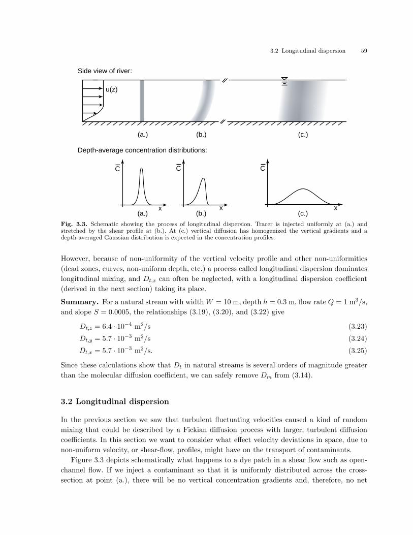
3.2 Longitudinal dispersion 59
u(z)
(a.) (b.) (c.)
Side view of river:
Depth-average concentration distributions:
x
C
x
C
x
C
(a.) (b.) (c.)
Fig. 3.3. Schematic showing the process of longitudinal dispersion. Tracer is injected uniformly at (a.) andstretched by the shear profile at (b.). At (c.) vertical diffusion has homogenized the vertical gradients and adepth-averaged Gaussian distribution is expected in the concentration profiles.
However, because of non-uniformity of the vertical velocity profile and other non-uniformities
(dead zones, curves, non-uniform depth, etc.) a process called longitudinal dispersion dominates
longitudinal mixing, and Dt,x can often be neglected, with a longitudinal dispersion coefficient
(derived in the next section) taking its place.
Summary. For a natural stream with width W = 10 m, depth h = 0.3 m, flow rate Q = 1 m3/s,
and slope S = 0.0005, the relationships (3.19), (3.20), and (3.22) give
Dt,z = 6.4 · 10−4 m2/s (3.23)
Dt,y = 5.7 · 10−3 m2/s (3.24)
Dt,x = 5.7 · 10−3 m2/s. (3.25)
Since these calculations show that Dt in natural streams is several orders of magnitude greater
than the molecular diffusion coefficient, we can safely remove Dm from (3.14).
3.2 Longitudinal dispersion
In the previous section we saw that turbulent fluctuating velocities caused a kind of random
mixing that could be described by a Fickian diffusion process with larger, turbulent diffusion
coefficients. In this section we want to consider what effect velocity deviations in space, due to
non-uniform velocity, or shear-flow, profiles, might have on the transport of contaminants.
Figure 3.3 depicts schematically what happens to a dye patch in a shear flow such as open-
channel flow. If we inject a contaminant so that it is uniformly distributed across the cross-
section at point (a.), there will be no vertical concentration gradients and, therefore, no net

60 3. Mixing in Rivers: Turbulent Diffusion and Dispersion
diffusive flux in the vertical at that point. The patch of tracer will advect downstream and
get stretched due to the different advection velocities in the shear profile. After some short
distance downstream, the patch will look like that at point (b.). At that point there are strong
vertical concentration gradients, and therefore, a large net diffusive flux in the vertical. As the
stretched out patch continues downstream, (turbulent) diffusion will smooth out these vertical
concentration gradients, and far enough downstream, the patch will look like that at point (c.).
The amount that the patch has spread out in the downstream direction at point (c.) is much more
than what could have been produced by just longitudinal (turbulent) diffusion. This combined
process of advection and vertical diffusion is called dispersion.
If we solve the transport equation in three dimensions using the appropriate molecular or
turbulent diffusion coefficients, we do not need to do anything special to capture the stretching ef-
fect of the velocity profile described above. Dispersion is implicitly included in three-dimensional
models.
However, we would like to take advantage of the fact that the concentration distribution
at the point (c.) is essentially one-dimensional: it is well mixed in the y- and z-directions. In
addition, the concentration distribution at point (c.) is observed to be Gaussian, suggesting a
Fickian-type diffusive process. Taylor’s analysis for dispersion, as presented in the following, is
a method to include the stretching effects of dispersion in a one-dimensional model. The result
is a one-dimensional transport equation with an enhanced longitudinal mixing coefficient, called
the longitudinal dispersion coefficient.
As pointed out by Fischer et al. (1979), the analysis presented by G. I. Taylor to compute
the longitudinal dispersion coefficient from the shear velocity profile is a particularly impressive
example of the genius of G. I. Taylor. At one point we will cancel out the terms of the equation
for which we are trying to solve. Through a scale analysis we will discard terms that would be
difficult to evaluate. And by thoroughly understanding the physics of the problem, we will use
a steady-state assumption that will make the problem tractable. Hence, just about all of our
mathematical tools will be used.
3.2.1 Derivation of the advective dispersion equation
To derive an equation for longitudinal dispersion, we will follow a modified version of the
Reynolds decomposition introduced in the previous section to handle turbulence. Referring to
Figure 3.4, we see that for one component of the turbulent decomposition, we have a mean
velocity that is constant at a point xi in three dimensional space and fluctuating velocities that
are variable in time so that
u(xi, t) = u(xi) + u′(xi, t). (3.26)
For shear-flow decomposition (here, we show the log-velocity profile in a river), we have a mean
velocity that is constant over the depth and deviating velocities that are variable over the depth
such that
u(z) = u + u′(z) (3.27)

3.2 Longitudinal dispersion 61
u'(t)
u
u
t
Reynolds Decomposition:turbulence
u'(z)
z
u u
Reynolds Decomposition:shear-flow
Fig. 3.4. Comparison of the Reynolds decomposition for turbulent flow (left) and shear flow (right).
where the over-bar represents a depth average, not an average o turbulent fluctuations. We
explicitly assume that u and u′(z) are independent of x. A main difference between these two
equations is that (3.26) has a random fluctuating component u′(xi, t); whereas, (3.27) has a
deterministic, non-random (and fully known!) fluctuating component u′(z), which we rather
call a deviation than a fluctuation. As for turbulent diffusion above, we also have a Reynold’s
decomposition for the concentrations
C(x, z) = C(x) + C ′(x, z) (3.28)
which is dependent on x, and for which C ′(x, z) is unknown.
Armed with these concepts, we are ready to follow Taylor’s analysis and apply it to longi-
tudinal dispersion in an open channel. For this derivation we will assume laminar flow and an
infinitely wide channel with no-flux boundaries at the top and bottom, so that v = w = 0. The
dye patch is introduced as a plane so that we can neglect lateral diffusion (∂C/∂y = 0). The
governing advective diffusion equation is
∂C
∂t+ u
∂C
∂x= Dx
∂2C
∂x2+ Dz
∂2C
∂z2. (3.29)
This equation is valid in three dimensions and contains the effect of dispersion. The diffusion
coefficients would either be molecular or turbulent, depending on whether the flow is laminar or
turbulent. Substituting the Reynolds decomposition for the shear velocity profile, we obtain
∂(C + C ′)
∂t+ (u + u′)
∂(C + C ′)
∂x= Dx
∂2(C + C ′)
∂x2+ Dz
∂2(C + C ′)
∂z2. (3.30)
Since we already argued that longitudinal dispersion will be much greater than longitudinal
diffusion, we will neglect the Dx-term for brevity (it can always be added back later as an
additive diffusion term). Also, note that C is not a function of z; thus, it drops out of the final
Dz-term.
As usual, it is easier to deal with this equation in a frame of reference that moves with the
mean advection velocity; thus, we introduce the coordinate transformation

62 3. Mixing in Rivers: Turbulent Diffusion and Dispersion
ξ = x − ut (3.31)
τ = t (3.32)
z = z, (3.33)
and using the chain rule, the differential operators become
∂
∂x=
∂
∂ξ
∂ξ
∂x+
∂
∂τ
∂τ
∂x+
∂
∂z
∂z
∂x
=∂
∂ξ(3.34)
∂
∂t=
∂
∂ξ
∂ξ
∂t+
∂
∂τ
∂τ
∂t+
∂
∂z
∂z
∂t
=∂
∂τ− u
∂
∂ξ(3.35)
∂
∂z=
∂
∂ξ
∂ξ
∂z+
∂
∂τ
∂τ
∂z+
∂
∂z
∂z
∂z
=∂
∂z. (3.36)
Substituting this transformation and combining like terms (and dropping the terms discussed
above) we obtain
∂(C + C ′)
∂τ+
∂u′(C + C ′)
∂ξ= Dz
∂2C ′
∂z2, (3.37)
which is effectively our starting point for Taylor’s analysis.
The discussion above indicates that it is the gradients of concentration and velocity in the
vertical that are responsible for the increased longitudinal dispersion. Thus, we would like, at
this point, to remove the non-fluctuating terms (terms without a prime) from (3.37). This step
takes great courage and profound foresight, since that means getting rid of ∂C/∂t, which is the
quantity we would ultimately like to predict (Fischer et al. 1979). As we will see, however, this
is precisely what enables us to obtain an equation for the dispersion coefficient.
To remove the constant components from (3.37), we will take the depth average of (3.37) and
then subtract that result from (3.37). The depth-average operator is
1
h
∫ h
0dz. (3.38)
Applying the depth average to (3.37) leaves
∂C
∂τ+
∂u′C ′
∂ξ= 0, (3.39)
since the depth average of C ′ is zero, but the cross-term, u′C ′, may not be zero. This equation is
the one-dimensional governing equation we are looking for. We will come back to this equation
once we have found a relationship for u′C ′. Subtracting this result from (3.37), we obtain
∂C ′
∂τ+ u′∂C
∂ξ+ u′∂C ′
∂ξ=
∂u′C ′
∂ξ+ Dz
∂2C ′
∂z2, (3.40)

3.2 Longitudinal dispersion 63
which gives us a governing equation for the concentration deviations C ′. If we can solve this
equation for C ′, then we can substitute the solution into (3.39) to obtain the desired equation
for C.
Before we solve (3.40), let us consider the scale of each term and decide whether it is necessary
to keep all the terms. This is called a scale-analysis. We are seeking solutions for the point (c.)
in Figure 3.3. At that point, a particle in the cloud has thoroughly sampled the velocity profile,
and C ′ C. Thus,
u′∂C ′
∂ξ u′∂C
∂ξand (3.41)
∂u′C ′
∂ξ u′∂C
∂ξ. (3.42)
We can neglect the two terms on the left-hand-side of the inequalities above, leaving us with
∂C ′
∂τ+ u′∂C
∂ξ= Dz
∂2C ′
∂z2. (3.43)
This might be another surprise. In the turbulent diffusion case, it was the cross-term u′C ′ that
became our turbulent diffusion term. Here, we have just discarded this term. In turbulence (as
will also be the case here for dispersion), that cross-term represents mass transport due to the
fluctuating velocities. But let us, also, take a closer look at the middle term of (3.43). This
term is an advection term working on the mean concentration, C, but due to the non-random
deviating velocity, u′(z). Thus, it is the transport term that represents the action of the shear
velocity profile.
Next, we see another insightful simplification that Taylor made. In the beginning stages of dis-
persion ((a.) and (b.) in Figure 3.3) the concentration fluctuations are unsteady, but downstream
(at point (c.)), after the velocity profile has been thoroughly sampled, the vertical concentration
fluctuations will reach a steady state (there will be a balanced vertical transport of contami-
nant), which represents the case of a constant (time-invariant) dispersion coefficient. At steady
state, (3.43) becomes
u′∂C
∂ξ=
∂
∂z
(
Dz∂C ′
∂z
)
(3.44)
where we have written the form for a non-constant Dz. Solving for C ′ by integrating twice gives
C ′(z) =∂C
∂ξ
∫ z
0
1
Dz
∫ z
0u′dzdz, (3.45)
which looks promising, but still contains the unknown C-term.
Step back for a moment and consider what the mass flux in the longitudinal direction is. In
our moving coordinate system, we only have one velocity; thus, the advective mass flux must be
qa = u′(C + C ′). (3.46)
To obtain the total mass flux, we take the depth average
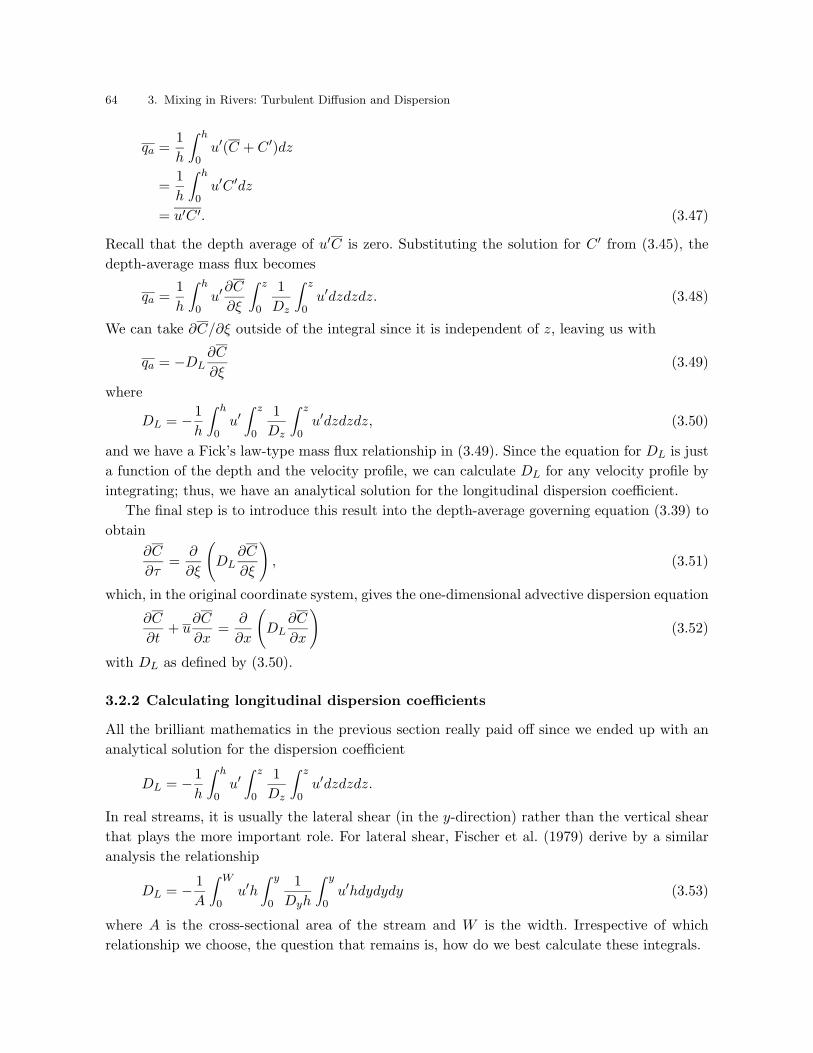
64 3. Mixing in Rivers: Turbulent Diffusion and Dispersion
qa =1
h
∫ h
0u′(C + C ′)dz
=1
h
∫ h
0u′C ′dz
= u′C ′. (3.47)
Recall that the depth average of u′C is zero. Substituting the solution for C ′ from (3.45), the
depth-average mass flux becomes
qa =1
h
∫ h
0u′∂C
∂ξ
∫ z
0
1
Dz
∫ z
0u′dzdzdz. (3.48)
We can take ∂C/∂ξ outside of the integral since it is independent of z, leaving us with
qa = −DL∂C
∂ξ(3.49)
where
DL = −1
h
∫ h
0u′∫ z
0
1
Dz
∫ z
0u′dzdzdz, (3.50)
and we have a Fick’s law-type mass flux relationship in (3.49). Since the equation for DL is just
a function of the depth and the velocity profile, we can calculate DL for any velocity profile by
integrating; thus, we have an analytical solution for the longitudinal dispersion coefficient.
The final step is to introduce this result into the depth-average governing equation (3.39) to
obtain
∂C
∂τ=
∂
∂ξ
(
DL∂C
∂ξ
)
, (3.51)
which, in the original coordinate system, gives the one-dimensional advective dispersion equation
∂C
∂t+ u
∂C
∂x=
∂
∂x
(
DL∂C
∂x
)
(3.52)
with DL as defined by (3.50).
3.2.2 Calculating longitudinal dispersion coefficients
All the brilliant mathematics in the previous section really paid off since we ended up with an
analytical solution for the dispersion coefficient
DL = −1
h
∫ h
0u′∫ z
0
1
Dz
∫ z
0u′dzdzdz.
In real streams, it is usually the lateral shear (in the y-direction) rather than the vertical shear
that plays the more important role. For lateral shear, Fischer et al. (1979) derive by a similar
analysis the relationship
DL = − 1
A
∫ W
0u′h
∫ y
0
1
Dyh
∫ y
0u′hdydydy (3.53)
where A is the cross-sectional area of the stream and W is the width. Irrespective of which
relationship we choose, the question that remains is, how do we best calculate these integrals.

3.2 Longitudinal dispersion 65
Example Box 3.3:River mixing processes.
As part of a dye study to estimate the mixing co-efficients in a river, a student injects a slug (pointsource) of dye at the surface of a stream in the mid-dle of the cross-section. Discuss the mixing processesand the length scales affecting the injected tracer.
Although the initial vertical momentum of the dyeinjection generally results in good vertical mixing,assume here that the student carefully injects thedye just at the stream surface. Vertical turbulentdiffusion will mix the dye over the depth, and fromExample Box 3.2 above, the injection can be treatedas mixed in the vertical after the point
Lz = 12h
where h is the stream depth.
As the dye continues to move downstream, lat-eral turbulent diffusion mixes the dye in the trans-verse direction. Based on the discussion in ExampleBox 3.2, the tracer can be considered well mixed lat-erally after
Ly =W 2
3h
where W is the stream width.For the region between the injection and Lz, the
dye cloud is fully three-dimensional, and no simplifi-cations can be made to the transport equation. Be-yond Lz, the cloud is vertically mixed, and longitudi-nal dispersion can be applied. For distances less thanLy, a two-dimensional model with lateral turbulentdiffusion and longitudinal dispersion is required. Fordistances beyond Ly, a one-dimensional longitudinaldispersion model is acceptable.
Analytical solutions. For laminar flows, analytical velocity profiles may sometimes exist and
(3.50) can be calculated analytically. Following examples in Fischer et al. (1979), the simplest
flow is the flow between two infinite plates, where the top plate is moving at U relative to the
bottom plate. For that case
DL =U2d2
120Dz(3.54)
where d is the distance between the two plates. Similarly, for laminar pipe flow, the solution is
DL =a2U2
0
192Dr(3.55)
where a is the pipe radius, U0 is the pipe centerline velocity and Dr is the radial diffusion
coefficient.
For turbulent flow, an analysis similar to the section on turbulent diffusion can be carried
out and the result is that (3.50) keeps the same form, and we substitute the turbulent diffusion
coefficient and the mean turbulent shear velocity profile for Dz and u′. The result for turbulent
flow in a pipe becomes
DL = 10.1au∗. (3.56)
One result of particular importance is that for an infinitely wide open channel of depth h.
Using the log-velocity profile (3.18) with von Karman constant κ = 0.4 and the relationship
(3.50), the dispersion coefficient is
DL = 5.93hu∗. (3.57)
Comparing this equation to the prediction for longitudinal turbulent diffusion from the previous
section (Dt,x = 0.15hu∗) we see that DL has the same form (∝ hu∗) and that DL is indeed much
greater than longitudinal turbulent diffusion. For real open channels, the lateral shear velocity
profile between the two banks becomes dominant and the leading coefficient for DL can range
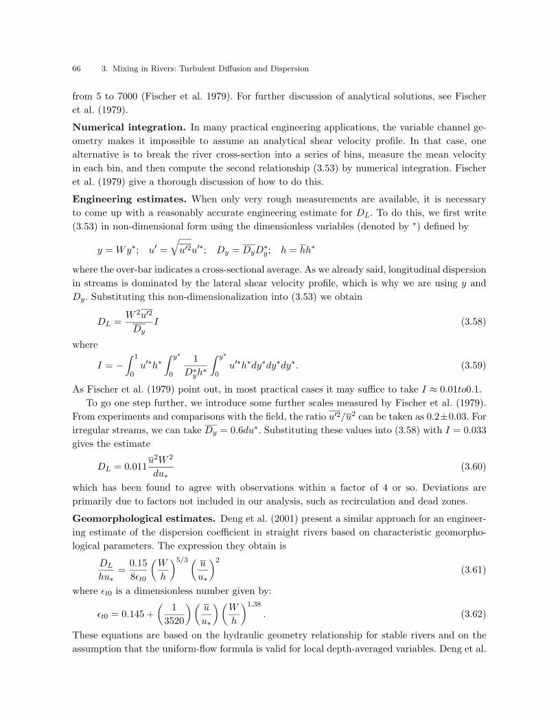
66 3. Mixing in Rivers: Turbulent Diffusion and Dispersion
from 5 to 7000 (Fischer et al. 1979). For further discussion of analytical solutions, see Fischer
et al. (1979).
Numerical integration. In many practical engineering applications, the variable channel ge-
ometry makes it impossible to assume an analytical shear velocity profile. In that case, one
alternative is to break the river cross-section into a series of bins, measure the mean velocity
in each bin, and then compute the second relationship (3.53) by numerical integration. Fischer
et al. (1979) give a thorough discussion of how to do this.
Engineering estimates. When only very rough measurements are available, it is necessary
to come up with a reasonably accurate engineering estimate for DL. To do this, we first write
(3.53) in non-dimensional form using the dimensionless variables (denoted by ∗) defined by
y = Wy∗; u′ =
√
u′2u′∗; Dy = DyD∗y; h = hh∗
where the over-bar indicates a cross-sectional average. As we already said, longitudinal dispersion
in streams is dominated by the lateral shear velocity profile, which is why we are using y and
Dy. Substituting this non-dimensionalization into (3.53) we obtain
DL =W 2u′2
DyI (3.58)
where
I = −∫ 1
0u′∗h∗
∫ y∗
0
1
D∗yh
∗
∫ y∗
0u′∗h∗dy∗dy∗dy∗. (3.59)
As Fischer et al. (1979) point out, in most practical cases it may suffice to take I ≈ 0.01to0.1.
To go one step further, we introduce some further scales measured by Fischer et al. (1979).
From experiments and comparisons with the field, the ratio u′2/u2 can be taken as 0.2±0.03. For
irregular streams, we can take Dy = 0.6du∗. Substituting these values into (3.58) with I = 0.033
gives the estimate
DL = 0.011u2W 2
du∗(3.60)
which has been found to agree with observations within a factor of 4 or so. Deviations are
primarily due to factors not included in our analysis, such as recirculation and dead zones.
Geomorphological estimates. Deng et al. (2001) present a similar approach for an engineer-
ing estimate of the dispersion coefficient in straight rivers based on characteristic geomorpho-
logical parameters. The expression they obtain is
DL
hu∗=
0.15
8εt0
(
W
h
)5/3 ( u
u∗
)2
(3.61)
where εt0 is a dimensionless number given by:
εt0 = 0.145 +
(
1
3520
)(
u
u∗
)(
W
h
)1.38
. (3.62)
These equations are based on the hydraulic geometry relationship for stable rivers and on the
assumption that the uniform-flow formula is valid for local depth-averaged variables. Deng et al.

3.3 Application: Dye studies 67
(2001) compare predictions for this relationship and predictions from (3.60) with measurements
from 73 sets of field data. More than 64% of the predictions by (3.61) fall within the range of
0.5 ≤ DL|prediction/DL|measurement ≤ 2. This accuracy is on average better than that for (3.60);
however, in some individual cases, (3.60) provides the better estimate.
Dye studies. One of the most reliable means of computing a dispersion coefficient is through
a dye study, as illustrated in the applications of the next sections. It is important to keep in
mind that since DL is dependent on the velocity profile, it is, in general, a function of the flow
rate. Hence, a DL computed by a dye study for one flow rate does not necessarily apply to a
situation at a much different flow rate. In such cases, it is probably best to perform a series of
dye studies over a range of flow rates, or to compare estimates such as (3.60) to the results of
one dye study to aid predictions under different conditions.
3.3 Application: Dye studies
The purpose of a dye tracer study is to determine a river’s flow and transport properties; in
particular, the mean advective velocity and the effective longitudinal dispersion coefficient. To
estimate these quantities, we inject dye upstream, measure the concentration distribution down-
stream, and compare the results to analytical solutions. The two major types of dye injections
are instantaneous injections and continuous injections. The following sections discuss typical
results for these two injection scenarios.
3.3.1 Preparations
To prepare a dye injection study, we use engineering estimates for the expected transport prop-
erties to determine the location of the measurement station(s), the duration of the experiment,
the needed amount of dye, and the type of dye injection.
For illustration purposes, assume in the following discussion that you measure a river cross-
section to have depth h = 0.35 m and width W = 10 m. The last time you visited the site, you
measured the surface current by timing leaves floating at the surface and found Us = 53 cm/s. A
rule-of-thumb for the mean stream velocity is U = 0.85Us = 0.45 cm/s. You estimate the river
slope from topographic maps as S = 0.0005. The channel is uniform but has some meandering.
Measurement stations. A critical part of a dye study is that you measure far enough down-
stream that the dye is well mixed across the cross-section. If you measure too close to the source,
you might obtain a curve for C(t) that looks Gaussian, but the concentrations will not be uni-
form across the cross-section, and dilution estimates will be biased. We use our mixing length
rules of thumb to compute the necessary downstream distance.
Assuming the injection is at a point (conservative case), it must mix both vertically and
transversely. The two relevant turbulent diffusion coefficients are
Dt,z = 0.067d√
gdS
= 9.7 · 10−4 m2/s (3.63)
68 3. Mixing in Rivers: Turbulent Diffusion and Dispersion
Dt,y = 0.6d√
gdS
= 8.7 · 10−3 m2/s. (3.64)
The time it takes for diffusion to spread a tracer over a distance l is l2/(12.5D); thus, the distance
the tracer would move downstream in this time is
Lx =l2
12.5DU. (3.65)
There are several injection possibilities. If you inject at the bottom or surface, the dye must
spread over the whole depth; if you inject at middle depth, the dye must only spread over half
the depth. Similarly, if you inject at either bank, the dye must spread across the whole river;
if you inject at the stream centerline, the dye must only spread over half the width. Often it
is possible to inject the dye in the middle of the river and at the water surface. For such an
injection, we compute in our example that Lm,z for spreading over the full depth is 4.2 m,
whereas, Lm,y for spreading over half the width is 95 m. Thus, the measuring station must be
at least Lm = 100 m downstream of the injection.
The longitudinal spreading of the cloud is controlled by the dispersion coefficient. Using the
estimate from Fischer et al. (1979) given in (3.60), we have
DL = 0.011U2W 2
d√
gdS
= 15.4 m2/s. (3.66)
We would like the longitudinal width of the cloud at the measuring station to be less than the
distance from the injection to the measuring station; thus, we would like a Peclet number, Pe,
at the measuring station of 0.1 or less. This criteria gives us
Lm =D
UPe= 342 m. (3.67)
Since for this stream the Peclet criteria is more stringent than that for lateral mixing, we chose
a measurement location of Lm = 350 m.
Experiment duration. We must measure downstream long enough in time to capture all of
the cloud or dye front as it passes. The center of the dye front reaches the measuring station
with the mean river flow: tc = Lc/U . Dispersion causes some of the dye to arrive earlier and
some of the dye to arrive later. An estimate for the length of the dye cloud that passes after the
center of mass is
Lσ = 3√
2DLLm/U
= 525 m (3.68)
or in time coordinates, tσ = 1170 s. Thus, we should start measuring immediately after the dye
is injected and continue taking measurements until t = tc + tσ = 30 min. To be conservative, we
select a duration of 35 min.
3.3 Application: Dye studies 69
Amount of injected dye tracer. The general public does not like to see red or orange water
in their rivers, so when we do a tracer study, we like to keep the concentration of dye low enough
that the water does not appear colored to the naked eye. This is possible using fluorescent dyes
because they remain visible to measurement devices at concentrations not noticeable to casual
observation. The most common fluorescent dye used in river studies is Rhodamine WT. Many
other dyes can also be used, including other types of Rhodamine (B, 6G, etc.) or Fluorescein.
Smart & Laidlay (1977) discuss the properties of many common fluorescent dyes.
In preparing a dye study, it is necessary to determine the amount (mass) of dye to inject. A
common field fluorometer by Turner Designs has a measurement range for Rhodamine WT of
(0.04 to 40)·10−2 mg/l. To have good sensitivity and also leave room for a wide range of river
flow rates, you should design for a maximum concentration at the measurement station near the
upper range of the fluorometer, for instance Cmax = 4 mg/l.
The amount of dye to inject depends on whether the injection is a point source or a continuous
injection. For a point source injection, we use the instantaneous point source solution with the
longitudinal dispersion coefficient estimated above
M = CmaxA√
4πDLLm/U
= 5.4 g. (3.69)
For a continuous injection, we estimate the dye mass flow rate from the expected dilution
m = U0ArCmax
= 6.3 g/s. (3.70)
These calculations show that a continuous release uses much more dye than a point release.
These estimates are for the pure (usually a powder) form of the dye.
Type of injection. To get the best injection characteristics, we dissolve the powder form of
the dye in a solution of water and alcohol before injecting it in the river. The alcohol is used to
obtain a neutrally buoyant mixture of dye. For a point release, we usually spill a bottle of dye
mixture containing the desired initial mass of dye in the center of the river and record the time
when the injection occurs. For a continuous release, we require some tubing to direct the dye
into the river, a reservoir containing dye at a known concentration, and a means of regulating
the flow rate of dye.
The easiest way to get a constant dye flow rate is to use a peristaltic pump. Another means
is to construct a Marriot bottle as described in Fischer et al. (1979) and shown in Figure 3.5.
The idea of the Marriot bottle is to create a constant head tank where you can assume the
pressure is equal to atmospheric pressure at the bottom of the vertical tube. As long as the
bottle has enough dye in it that the bottom of the vertical tube is submerged, a constant flow
rate Q0 will result by virtue of the constant pressure head between the tank and the injection.
We must calibrate the flow rate in the laboratory for a given head drop prior to conducting the
field experiment.
The concentration of the dye C0 for the continuous release is calculated according to the
equation

70 3. Mixing in Rivers: Turbulent Diffusion and Dispersion
Fig. 3.5. Schematic of a Marriot bottle taken from Fischer et al. (1979).
0 5 10 15 20 25 30 350
0.5
1
1.5
2
2.5
3
3.5Measured dye concentration breakthrough curve
Time since injection start [min]
Con
cent
ratio
n [m
g/l]
Fig. 3.6. Measured dye concentration for example dye study. Dye fluctuations are due to instrument uncertainty,not due to turbulent fluctuations.
m = Q0C0 (3.71)
where Q0 is the flow rate from the pump or Marriot bottle. With these design issues complete,
a dye study is ready to be conducted.
3.3.2 River flow rates
Figure 3.6 shows a breakthrough curve for a continuous injection, based on the design in the
previous section. The river flow rate can be estimated from the measured steady-state concen-
tration in the river Cr at t = 35 min. Reading from the graph, we have Cr = 3.15 mg/l. Thus,
the actual flow rate measured in the dye study was
Qr =m
Cr
= 2.0 m3/s. (3.72)

3.4 Application: Dye study in Cowaselon Creek 71
Notice that this estimate for the river flow rate is independent of the cross-sectional area.
To estimate the error in this measurement, we use the error-propagation equation
δγ =
√
√
√
√
n∑
i=1
(
∂γ
∂miδmi
)2
(3.73)
where δγ is the error in some quantity γ, estimated from n measurements mi. Computing the
error for our river flow rate estimate, we have
δQr =
√
(
C0
CrδQ0
)2
+
(
Q0
CrδC0
)2
+
(
Q0C0
C2r
δCr
)2
. (3.74)
If the uncertainties in the measurements were Cr = (3.15 ± 0.04) mg/l, C0 = 32 ± 0.01 g/l and
Q0 = 0.2 ± 0.01 l/s, then our estimate should be Qr = 2.0 ± 0.1 m3/s. The error propagation
formula is helpful for determining which sources of error contribute the most to the overall error
in our estimate.
3.3.3 River dispersion coefficients
The breakthrough curve in Figure 3.6 also contains all the information we need to estimate an
in situ longitudinal dispersion coefficient. To do that, we will use the relationship
σ2 = 2DLt. (3.75)
Since our measurements of σ are in time, we must convert them to space in order to use this
equation. One problem is that the dye cloud continues to grow as it passes the site, so the width
measured at the beginning of the front is less than the width measured after most of the front
has passed; thus, we must take an average.
The center of the dye front can be taken at C = 0.5C0, which passed the station at
t = 12.94 min and represents the mean stream velocity. One standard deviation to the left
of this point is at C = 0.16C0, as shown in the figure. This concentration passed the measure-
ment station at t = 8.35 min. One standard deviation to the right is at C = 0.84C0, and this
concentration passed the station at t = 20.12 min. From this information, the average velocity
is u = 0.45 m/s and the average width of the front is 2σt = 20.12− 8.35 = 11.77 min. The time
associated with this average sigma is t = 8.35 + 11.77/2 = 14.24 min.
To compute DL from (3.75), we must convert our time estimate of σt to a spatial estimate
using σ = uσt. Solving for DL gives
DL =u2σ2
t
2t= 14.8 m2/s. (3.76)
This value compares favorably with our initial estimate from (3.50) of 15.4 m2/s.
3.4 Application: Dye study in Cowaselon Creek
In 1981, students at Cornell University performed a dye study in Cowaselon Creek using an
instantaneous point source of Rhodamine WT dye. The section of Cowaselon Creek tested has

72 3. Mixing in Rivers: Turbulent Diffusion and Dispersion
a very uniform cross-section and a straight fall line from the injection point through the mea-
surement stations. At the injection site, the students measured the cross-section and flow rate,
obtaining
Q = 0.6 m3/s W = 10.7 m
u = 0.17 m/s h = 0.3 m.
From topographic maps, they measured the creek slope over the study area to be S = 4.3 ·10−4.
The concentration profiles were measured at three stations downstream. The first station was
670 m downstream of the injection, the second station was 2800 m downstream of the injection,
and the final station was 5230 m downstream of the injection. At each location, samples were
taken in the center of the river and near the right and left banks. Figure 3.7 shows the measured
concentration profiles.
For turbulent mixing in the vertical direction, the downstream distance would be Lm,z =
12d = 17 m. This location is well upstream of our measurements; thus, we expect the plume to
be well-mixed in the vertical by the time it reaches the measurement stations.
For mixing in the lateral direction, the method in Example Box 3.3 (using Dt,y = 0.15du∗ for
straight channels) gives a downstream distance of Lm,y = 2500 m. Since the first measurement
station is at L = 670 m we clearly see that there are still lateral gradients in the concentra-
tion cloud. At the second measurement station, 2800 m downstream, the lateral gradients have
diffused, and the lateral distribution is independent of the lateral coordinate. Likewise, at the
third measurement station, 5230 m downstream, the plume is mixed laterally; however, due to
dispersion, the plume has also spread more in the longitudinal direction.
To estimate the dispersion coefficient, we can take the travel time between the stations two
and three and the growth of the cloud. The travel time between stations is δt = 3.97 hr. The
width at station one is σ1 = 236 m, and the width at station two is σ2 = 448 m. The dispersion
coefficient is
DL =σ2
2 − σ21
2δt= 5.1 m2/s. (3.77)
Comparing to (3.60) and (3.61), we compute
DL|Fischer = 3.4 m2/s (3.78)
DL|Deng = 5.4 m2/s. (3.79)
Although the geomorphological estimate of 5.4 m2/s is closer to the true value than is 3.3 m2/s,
for practical purposes, both methods give good results. Dye studies, however, are always helpful
for determining the true mixing characteristics of rivers.
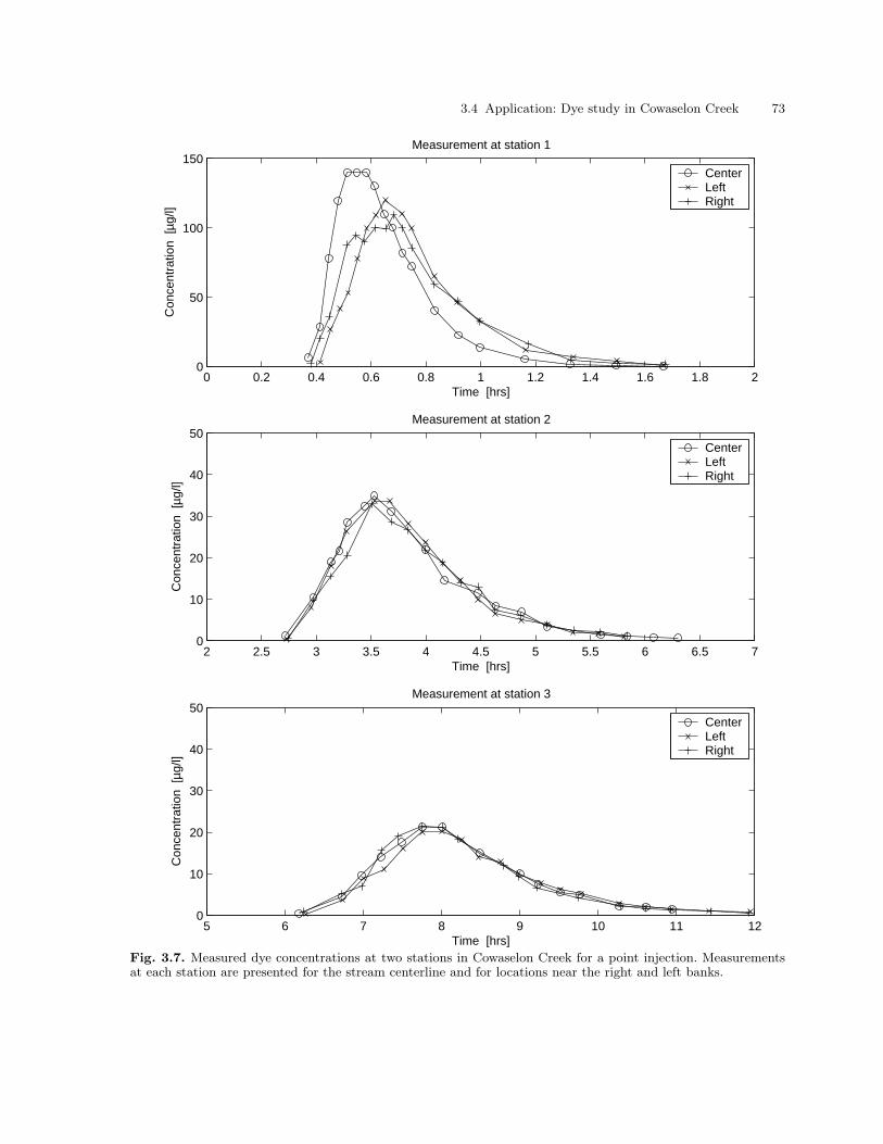
3.4 Application: Dye study in Cowaselon Creek 73
0 0.2 0.4 0.6 0.8 1 1.2 1.4 1.6 1.8 20
50
100
150C
once
ntra
tion
[µg/
l]
Time [hrs]
Measurement at station 1
2 2.5 3 3.5 4 4.5 5 5.5 6 6.5 70
10
20
30
40
50
Con
cent
ratio
n [µ
g/l]
Time [hrs]
Measurement at station 2
5 6 7 8 9 10 11 120
10
20
30
40
50
Con
cent
ratio
n [µ
g/l]
Time [hrs]
Measurement at station 3
CenterLeftRight
CenterLeftRight
CenterLeftRight
Fig. 3.7. Measured dye concentrations at two stations in Cowaselon Creek for a point injection. Measurementsat each station are presented for the stream centerline and for locations near the right and left banks.

74 3. Mixing in Rivers: Turbulent Diffusion and Dispersion
Summary
This chapter presented the effects of contaminant transport due to variability in the ambient
velocity. In the first section, turbulence was discussed and shown to be composed of a mean
velocity and a random, fluctuating turbulent velocity. By introducing the Reynolds decomposi-
tion of the turbulent velocity into the advective diffusion equation, a new equation for turbulent
diffusion was derived that has the same form as that for molecular diffusion, but with larger,
turbulent diffusion coefficients. The second type of variable velocity was a shear velocity profile,
described by a mean stream velocity and deterministic deviations from that velocity. Substitut-
ing a modified type of Reynolds decomposition for the shear profile into the advective diffusion
equation and depth averaging led to a new equation for longitudinal dispersion and an integral
relationship for calculating the longitudinal dispersion coefficient. To demonstrate how to use
these equations and obtain field measurements of these properties, the chapter closed with an
example of a simple dye study to obtain stream flow rate and longitudinal dispersion coefficient.
Exercises
3.1 Properties of turbulence. The axial velocity u of a turbulent jet can be measured using a
laser Doppler velocimetry (LDV) system. Obtain a data file that contains only one column (the
u component velocity) with a unit of m/s; the sampling rate is 100 Hz. Do the following:
• Plot the velocity and examine whether the flow is turbulent by checking the randomness in
your plot. Comment on your observations.
• Use Matlab to calculate the mean velocity and create a variable that contains just the fluctu-
ating velocity (you do not have to turn in anything for this step).
• Plot the fluctuating velocity.
• Calculate the mean value of the fluctuating velocity .
• Write a program to compute the correlation function (normalized so the maximum correlation
is 1.0) and plot the function.
• Calculate the integral time scale (integrate between 0 to 0.3 s only).
• Estimate the “typical” size of the eddies (find the integral length scale).
3.2 Turbulent diffusion coefficients. The Rhine river in the vicinity of Karlsruhe has width
B = 300 m and Manning’s friction factor 0.02. The slope is 1 · 10−4. Assume the river is always
at normal depth and that the width is constant for all flow rates.
• For each flow rate in Table 3.1, compute the dispersion coefficient from the equation from
Fischer et al. (1977)
DL = 0.011u2B2
hu∗(3.80)
where u is the mean velocity and u∗ is the shear velocity.

Exercises 75
Table 3.1. Flow rates in the Rhine river near Karlsruhe.
Flow rate
[m3/s]
120
240
500
800
1200
• For each flow rate in Table 3.1, compute the dispersion coefficient from the equation from
Deng et al. (2001)
DL
hu∗=
0.15
8εt0
(
B
h
)5/3 ( u
u∗
)2
(3.81)
with
εt0 = 0.145 +
(
1
3520
)(
u
u∗
)(
B
h
)1.38
. (3.82)
where h is the water depth and B is the channel width.
• Plot the dispersion coefficient for each method as a function of flow rate and comment on the
trends. Do you think it is adequate to do one dye study to evaluate DL? Why or why not?
3.3 Numerical integration. Using the velocity profile data in Table 3.2 (from Nepf (1995)),
perform a numerical integration of (3.53) to estimate a longitudinal dispersion coefficient. You
should obtain a value of DL = 1.5 m2/s.
3.4 Dye study. This problem is adapted from Nepf (1995). A small stream has been found to be
contaminated with Lindane, a pesticide known to cause convulsions and liver damage. Ground-
water wells in the same region have also been found to contain Lindane, and so you suspect
that the river contamination is due to groundwater inflow. To test your theory, you conduct a
dye study using a continuous release of dye. Based on the information given in Figure 3.8, what
is the groundwater volume flux and the concentration of Lindane in the groundwater between
Stations 2 and 3? The variables in the figure are Qd the volume flow rate of the dye at the
injection, Cd the concentration of the dye at the injection and at downstream stations, Cl the
concentration of Lindane in the river at each station, W the width of the river, and d the depth
in the river. (Hint: this is a steady-state problem, so you do not need to use diffusion coefficients
to solve the problem other than to determine whether the dye is well-mixed when it reaches
Station 2.)
Due to problems with the pump, the dye flow rate has an error of Qd = 100 ± 5 cm3/s.
Assume this is the only error in your measurement and report your measurement uncertainty.
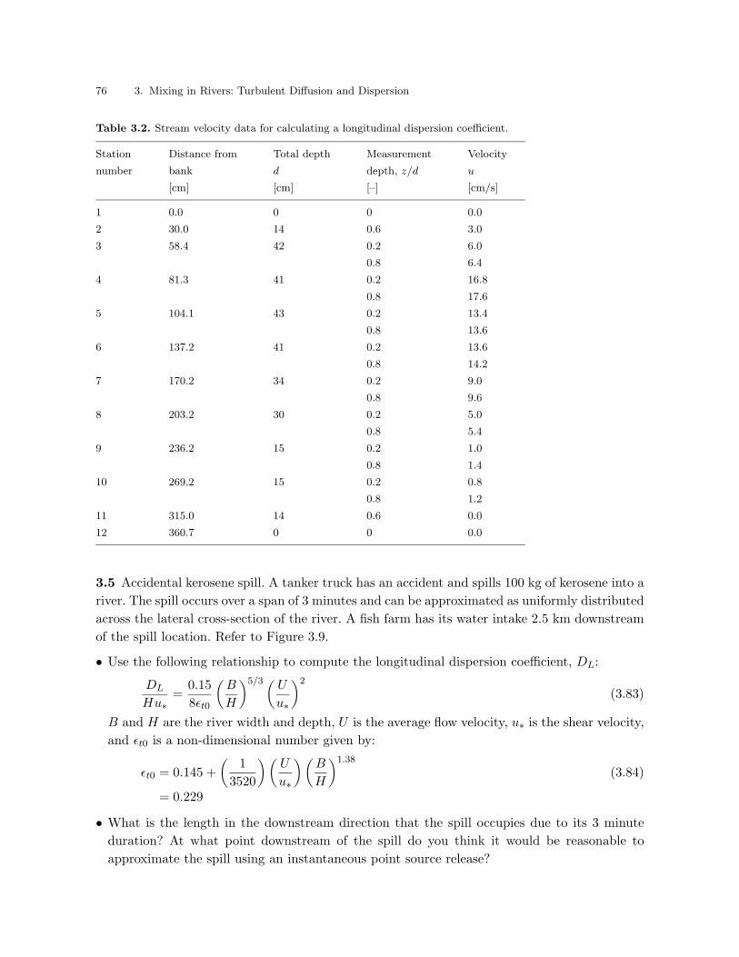
76 3. Mixing in Rivers: Turbulent Diffusion and Dispersion
Table 3.2. Stream velocity data for calculating a longitudinal dispersion coefficient.
Station Distance from Total depth Measurement Velocity
number bank d depth, z/d u
[cm] [cm] [–] [cm/s]
1 0.0 0 0 0.0
2 30.0 14 0.6 3.0
3 58.4 42 0.2 6.0
0.8 6.4
4 81.3 41 0.2 16.8
0.8 17.6
5 104.1 43 0.2 13.4
0.8 13.6
6 137.2 41 0.2 13.6
0.8 14.2
7 170.2 34 0.2 9.0
0.8 9.6
8 203.2 30 0.2 5.0
0.8 5.4
9 236.2 15 0.2 1.0
0.8 1.4
10 269.2 15 0.2 0.8
0.8 1.2
11 315.0 14 0.6 0.0
12 360.7 0 0 0.0
3.5 Accidental kerosene spill. A tanker truck has an accident and spills 100 kg of kerosene into a
river. The spill occurs over a span of 3 minutes and can be approximated as uniformly distributed
across the lateral cross-section of the river. A fish farm has its water intake 2.5 km downstream
of the spill location. Refer to Figure 3.9.
• Use the following relationship to compute the longitudinal dispersion coefficient, DL:
DL
Hu∗=
0.15
8εt0
(
B
H
)5/3 ( U
u∗
)2
(3.83)
B and H are the river width and depth, U is the average flow velocity, u∗ is the shear velocity,
and εt0 is a non-dimensional number given by:
εt0 = 0.145 +
(
1
3520
)(
U
u∗
)(
B
H
)1.38
(3.84)
= 0.229
• What is the length in the downstream direction that the spill occupies due to its 3 minute
duration? At what point downstream of the spill do you think it would be reasonable to
approximate the spill using an instantaneous point source release?
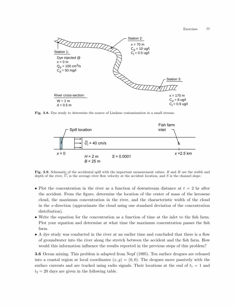
Exercises 77
Station 1:
Dye injected @x = 0 mQd = 100 cm3/sCd = 50 mg/l
x = 70 mCd = 10 ug/lCl = 0.5 ug/l
x = 170 mCd = 8 ug/lCl = 0.9 ug/l
Station 2:
Station 3:
River cross-section:
W = 1 md = 0.5 m
Fig. 3.8. Dye study to determine the source of Lindane contamination in a small stream.
Spill location
Fish farm
inlet
x = 0 x =2.5 km
Ui = 40 cm/s
H = 2 m
B = 25 m
S = 0.0001
Fig. 3.9. Schematic of the accidental spill with the important measurement values. B and H are the width anddepth of the river, Ui is the average river flow velocity at the accident location, and S is the channel slope.
• Plot the concentration in the river as a function of downstream distance at t = 2 hr after
the accident. From the figure, determine the location of the center of mass of the kerosene
cloud, the maximum concentration in the river, and the characteristic width of the cloud
in the x-direction (approximate the cloud using one standard deviation of the concentration
distribution).
• Write the equation for the concentration as a function of time at the inlet to the fish farm.
Plot your equation and determine at what time the maximum concentration passes the fish
farm.
• A dye study was conducted in the river at an earlier time and concluded that there is a flow
of groundwater into the river along the stretch between the accident and the fish farm. How
would this information influence the results reported in the previous steps of this problem?
3.6 Ocean mixing. This problem is adapted from Nepf (1995). Ten surface drogues are released
into a coastal region at local coordinates (x, y) = (0, 0). The drogues move passively with the
surface currents and are tracked using radio signals. Their locations at the end of t1 = 1 and
t2 = 20 days are given in the following table.

78 3. Mixing in Rivers: Turbulent Diffusion and Dispersion
Table 3.3. Drogue position data.
Drogue x(t1) y(t1) x(t2) y(t2)
Number [km] [km] [km] [km]
1 2.5 0.2 5.3 8.1
2 4.6 1.4 2.3 1.0
3 2.3 -1.2 6.6 3.9
4 3.1 -0.4 6.7 -2.8
5 1.5 0.8 0.5 4.2
6 1.4 2.1 10.1 3.6
7 4.7 2.1 6.6 -1.4
8 2.7 0.2 6.0 -2.9
9 1.5 2.6 3.2 2.1
10 4.9 2.3 -4.0 1.7
1. Estimate the advection velocity and the lateral coefficients of diffusion (Dx and Dy) for this
coastal region.
2. Using the radio links, the positions of all ten drogues can be collected within ten min-
utes. Suppose the radio link were to break down and the positions were instead determined
through visual observation. Even using a helicopter, it requires nearly four hours to locate
all ten drogues. How does this change the accuracy of your data? Can you still consider the
measurements to be synoptic?
3. Later, a freight ship is caught in a winter storm off the coast where this drogue study was
conducted. High winds and rough seas cause several shipping containers to be washed over-
board. One of the containers breaks open, releasing its contents: 29,000 children’s bathtub
toys. Estimate how long it will take for the toys to begin to wash up on shore assuming the
same transport characteristics as during the drogue study and that the spill occurs 1 km
off the coast. (This really happened in the Pacific Ocean, and the trajectory of the bathtub
toys, plastic turtles and ducks, were subsequently used to gain information about the current
system.)
3.7 Mixing of a continuous point source in a river. Many dye studies are conducted by injecting a
continuous point source of dye at one station and measuring the dilution at downstream stations,
where the dye is assumed to be well-mixed across the cross-section. The continuous point source
solution in an infinite domain with constant, uniform advection current in the x-direction, U , is
C(x, y, z) =m
4πx√
DzDyexp
(
−(z − z0)2U
4Dzx− (y − y0)
2U
4Dyx
)
(3.85)
where m is the mass flux of dye at the injection, x is the downstream distance, Dz is the
vertical diffusion coefficient, Dy is the lateral diffusion coefficient, z0 is the vertical position of
the injection, and y0 is the lateral position of the injection. To derive this solution, we have
assumed that longitudinal diffusion is negligible (called the slender-plume approximation).

Exercises 79
In a river there are four boundaries that must be accounted for. In the vertical direction, there
are boundaries at the channel bed and at the free-water surface. In the lateral direction, there
are boundaries at each channel bank. Write a Matlab function that solves this problem for an
arbitrary injection point at (0, y0, z0). It should take the vertical coordinate as positive upward
with origin at the channel bed and the lateral coordinate as positive toward the right-hand bank
with origin at the channel center-line.
Dimensional analysis can be used to estimate the distance Lm downstream of an injection at
x = 0 at which the injection may be considered well-mixed in the vertical or lateral direction.
This relationship is
Lm ∝ L2U
D(3.86)
where L is the distance over which the dye must spread (for vertical mixing, this would be the
water depth), Lm is the downstream distance to the point where the cloud can be considered
well-mixed, and D is the pertinent diffusion coefficient (for vertical mixing, this would be Dz). To
calibrate this relationship, we define “well-mixed” as the point at which the ratio of the minimum
dye concentration Cmin to the maximum dye concentration Cmax across the cross-section reaches
a threshold value. Common practice is to define well-mixed as Cmin/Cmax = 0.95. Using this
criteria, we can calculate Lm, and a proportionality constant α can be determined, giving the
relationship
Lm = αL2U
D. (3.87)
Use this information to study a river with the following characteristics:
• Width B = 10.7 m
• Depth H = 0.3 m
• Slope S = 4.3 · 10−4
• Mean flow velocity u = 0.17 m/s
• Dye injection rate m = 1 g/s;
Use enough image sources that your solution is independent of the number of images you are
using and answer the following questions:
1. What is the value of Manning’s roughness coefficient n that corresponds to the given flow
depth and channel slope? Do you think that this value is reasonable? If it seems too high
or too low, do you expect that the estimate for the shear velocity of u∗ =√
gHS is an
over-prediction or under-prediction for this stream? Use your calibrated value of n for the
remaining questions.
2. Plot the relative concentration C(x, 0, H)/C(x, 0, 0.5H) for an injection at (0, 0, 0.5H) versus
downstream distance for x between x = 1 m and x = 45 m.
3. Calibrate the coefficient α in (3.87) for vertical mixing for an injection at y0 = 0 and
z0 = [0, 0.25H, 0.5H, 0.75H, H] for the criteria C(z)min/C(z)max = 0.95.
4. Repeat your calculations in the previous step, but move the injection to y0 = B/2. Does this
affect your results? Why or why not?

80 3. Mixing in Rivers: Turbulent Diffusion and Dispersion
5. Calibrate the coefficient α in (3.87) for lateral mixing for an injection at z0 = 0.5H and
y0 = [B/2, B/4, 0,−B/4,−B/2] for the criteria C(y)min/C(y)max = 0.95. Do you think
your results would change if you moved the injection at z0 to a different elevation? Why or
why not?
6. Repeat your calculations in the previous step, but using a lateral diffusion coefficient of
Dy = 0.6u∗H. Did this change your value of α?
7. Based on these results, what value of α would you recommend for an arbitrary injection
location (you must pick a single value of α that best represents your data).
(Hint: it would probably be a good idea to do your calculations by writing a second Matlab
program that solves the questions above. You can plot the relative concentration downstream
and use ginput to pick the point where Cmin/Cmax = 0.95).
4. Physical, Chemical, and Biological
Transformations
In the previous chapters, concentrations change in response to transport processes, such as
diffusion, advection, and dispersion, and we have considered these processes in mass conserving
systems. Now, we would like to look at systems where the mass of a given species of interest is
not conserving. Processes that remove mass can be physical, chemical or biological in nature.
Since the total mass of the system must be conserved, these processes generally change the
species of interest into another species; thus, we will call these processes transformation.
This chapter begins by describing the common types of transformation reactions. Since we
are interested in concentration changes, we review reaction kinetics and derive rate laws for
first- and second-order systems. The methods are then generalized to higher-order reactions.
Transformation is then added to our transport equation for two types of reactions. In the first
case, the reaction becomes a source or sink term in the governing differential equation; in the
second case, the reaction occurs at the boundary and becomes a boundary constraint on the
governing transport equation. The chapter closes with an engineering application to bacteria
die-off downstream of a wastewater treatment plant.
4.1 Concepts and definitions
Transformation is defined as production (or loss) of a given species of interest through physical,
chemical, or biological processes. When no transformation occurs, the system is said to be
conservative, and we represent this characteristic mathematically with the conservation of mass
equation
dMi
dt= 0 (4.1)
where Mi is the total mass of species i. When transformation does occur, the system is called
reactive, and, for a given species of interest, the system is no longer conservative. We represent
this characteristic mathematically as
dMi
dt= Si (4.2)
where Si is a source or sink term. For reactive systems, we must supply these reaction equations
that describe the production or loss of the species of interest. Since the total system mass must
be conserved, these reactions are often represented by a system of transformation equations.
Transformation reactions are broadly categorized as either homogeneous or heterogeneous.
Homogeneous reactions occur everywhere within the fluid of interest. This means that they are
Copyright c© 2004 by Scott A. Socolofsky and Gerhard H. Jirka. All rights reserved.

82 4. Physical, Chemical and Biological Transformations
distributed throughout the control volume; hence, they are represented as a source or sink term
in the governing differential equation. By contrast, heterogeneous reactions occur only at fluid
boundaries. They are not distributed throughout the control volume; hence, they are specified
by source or sink boundary conditions constraining the governing differential equation.
Some reactions have properties of both homogeneous and heterogeneous reactions. As an
example, consider a reaction that occurs on the surface of suspended sediment particles. Because
the reaction occurs only at the sediment/water interface, the reaction is heterogeneous. But,
because the sediment is suspended throughout the water column, the effect of the reaction is
homogeneous in nature. Models that represent the reaction through boundary conditions (i.e.
they treat the reaction as heterogeneous) are sometimes called two-phase, or multi-phase, models.
Models that simplify the reaction to treat it as a homogeneous reaction are called single-phase,
or mixture, models. To obtain analytical solutions, we often must use the single-phase approach.
4.1.1 Physical transformation
Physical transformations result from processes governed by the laws of physics. The classical
example, which comes from the field of nuclear physics, is radioactive decay. Radioactive decay is
the process by which an atomic nucleus emits particles or electromagnetic radiation to become
either a different isotope of the same element or an atom of a different element. The three
radioactive decay paths are alpha decay (the emission of a helium nucleus), beta decay (the
emission of an electron or positron), and gamma decay (the emission of a photon). Gamma
decay alone does not result in transformation, but it is generally accompanied by beta emission,
which does.
A common radioactive element encountered in civil engineering is radon, a species in the
uranium decay chain. Radon decays to polonium by alpha decay according to the equation
222Rn → 218Po + α (4.3)
where α represents the ejected helium nucleus, 42He. As we will see in the section on kinetics,
this single-step reaction is first order, and the concentration of radon decreases exponentially
with time. The time it takes for half the initial mass of radon to be transformed is called the
half-life.
Another common example that we will treat as a physical transformation is the settling of
suspended sediment particles. Although settling does not actually transform the sediment into
something else, it does remove sediment from our control volume by depositing it on the river
bed. This process can be expressed mathematically by heterogeneous transformation equations
at the river bed; hence, we will discuss it as a transformation.
4.1.2 Chemical transformation
Chemical transformation refers to the broad range of physical and organic chemical reactions
that do not involve transformations at the atomic level. Thus, the periodic table of the elements
contains all the building blocks of chemical transformations.

4.2 Reaction kinetics 83
A classic example from aqueous phase chemistry is the dissolution of carbon dioxide (CO2)
in water (H2O), given by the equilibrium equation
CO2 + H2O HCO−3 + H+ (4.4)
where HCO−3 is called bicarbonate and H+ is the hydrogen ion. The terms on the left-hand-side
of the equation are called the reactants; the terms on the right-hand-side of the equation are
called the products. Equilibrium refers to the state in which the formation of products occurs
at the same rate as the reverse process that re-forms the reactants from the products. This
give-and-take balance between reactants and products is indicated by the symbol.
4.1.3 Biological transformation
Biological transformation refers to that sub-set of chemical reactions mediated by living or-
ganisms through the processes of photosynthesis and respiration. These reactions involve the
consumption of a nutritive substance to produce biomass, and are accompanied by an input or
output of energy.
The classical photosynthesis equation shows the production of glucose, C6H12O6, from CO2
through the input of solar radiation, hν :
6CO2 + 6H2O → C6H12O6 + 6O2. (4.5)hν
Photosynthesis and respiration (particularly in the form of biodegradation) are of partic-
ular interest in environmental engineering because they affect the concentration of oxygen, a
component essential for most aquatic life.
4.2 Reaction kinetics
Reaction kinetics is the study of the rate of formation of products from reactants in a trans-
formation reaction. All reactions occur at a characteristic rate ∆tk. A common measure of this
characteristic rate is the half-life, the time for half of the reactants to be converted into products.
The other physical processes of interest in our problems (i.e. diffusion and advection) also occur
with characteristic time scales, ∆tp. Comparing these characteristic time-scales, three cases can
be identified:
• ∆tk ∆tp: For these reactions we can assume the products are formed as soon as reactants
become available, and we can neglect the reaction kinetics. Such reactions are called instanta-
neous and are reactant-limited; that is, the rate of formation of products is controlled by the
rate of formation of reactants and not by the reaction rate of the tranformation equation.
• ∆tk ∆tp: For these reactions the reaction can be ignored altogether, and we have a conser-
vative (non-reacting) system.
• ∆tk ≈ ∆tp: For these reactions neither the reaction nor the reaction kinetics can be ignored.
Assuming the products are readily available, such reactions are called rate-limited, and the rate
of formation of products is controlled by the reaction kinetics of the chemical transformation.

84 4. Physical, Chemical and Biological Transformations
This last case, where the reactions are rate-limited, is the case of interest in this chapter, and
in this section we discuss the rate laws of chemical kinetics.
To formulate the rate laws for a generic reaction, consider the mixed chemical reaction
aA + bB → cC + dD, (4.6)
where the lower-case letters are the stoichiometric coefficients of the reaction and the upper-case
letters are the reactants (A and B) and products (C and D). The general form of the rate law
for species A can be written as
d[A]
dt= RA, (4.7)
where RA is a function describing the rate law for species A. We use the [A]-notation to designate
concentration of species A (we will also use the equivalent notation CA). From the stoichiometry
of the reaction, the following ratios can also be inferred:
d[A]/dt
d[B]/dt=
a
b, and
d[A]/dt
−d[C]/dt=
a
c.
Substituting the rate laws gives the relationships
RA = +a
bRB, and (4.8)
RA = −a
cRC . (4.9)
We still require a means of writing the rate law for species i, Ri.
The general form of the rate law for product i formed from j reactants is
Ri = kiCn1
1 Cn2
2 ... Cnj
j , (4.10)
where k is the rate constant of the reaction, nj is the order of the reaction with respect to
constituent j, and K =∑j
i=1 ni is the overall reaction order (note that the units of k depend on
K). In general, reaction order cannot be predicted (except for simple, single-step, elementary
reactions, where reaction order is the stoichiometric coefficient). Hence, reaction rate laws are
determined on an experimental basis.
As one might expect, the reaction rate k is temperature dependent. One way to find a
relationship for k(T ) is to use Arrhenius equation for an ideal gas
k = A exp(−Ea/(RT )), (4.11)
where A is a constant, Ea is the activation energy, R is the ideal gas constant, and T is the
absolute temperature. Defining k1 = k(T1) we can rearrange this equation to obtain
k(T ) = k1 exp
(
Ea(T − T1)
RTT1
)
. (4.12)
for small temperature changes, this equation can be linearized by defining the constant
θ =Ea
RT2T1. (4.13)

4.2 Reaction kinetics 85
Then, for T1 ≤ T ≤ T2,
k(T ) = k1 exp(θ(T − T1)). (4.14)
This form of the temperature dependence is often applied to non-gaseous systems as well.
4.2.1 First-order reactions
The general equation for a first-order reaction is
dC
dt= ±kC, (4.15)
where k has units [1/T ]. Common examples are radioactive decay and the die-off of bacteria in
a river. Whether mass increases or decreases in our control volume depends on our perspective:
it depends on which species we are interested in, since one species will decrease as the other is
created. To avoid confusion, we will always report the rate constant for the reaction using an
absolute value. In this way, k is always positive. We then must chose the positive or negative sign
in (4.15) depending on whether the species of interest is increasing (positive sign) or decreasing
(negative sign) in our control volume.
This is a standard initial-value problem, whose solution can be found subject to the initial
condition
C(t = 0) = C0. (4.16)
First, rearrange the governing equation to obtain
dC
C= ±kdt. (4.17)
Next, integrate both sides, yielding∫
dC
C=
∫
±kdt
ln(C) = ±kt + C1, (4.18)
where C1 is an integration constant. Solving for C we obtain
C = C ′1 exp(±kt), (4.19)
where C ′1 is another constant (given by exp(C1)). After applying the initial condition, we obtain
C(t) = C0 exp(±kt). (4.20)
Figure 4.1 plots this solution for a decreasing concentration (negative sign in solution) for C0 = 1
and k = 1.
As already discussed above, the characteristic reaction time is given by the time it takes
for the ratio C(t)/C0 to reach a specified value. For radioactive decay, k is negative, and two
common characteristic times are the half-life and the e-folding time. The half-life, T1/2, is the
time required for the concentration ratio to reach 1/2. From (4.20), the half-life is
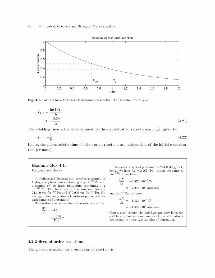
86 4. Physical, Chemical and Biological Transformations
0 0.2 0.4 0.6 0.8 1 1.2 1.4 1.6 1.8 20
0.2
0.4
0.6
0.8
1
T1/2 T
e
Solution for first−order reaction
Time
Con
cent
ratio
n
Fig. 4.1. Solution for a first-order transformation reaction. The reaction rate is k = −1.
T1/2 =ln(1/2)
k
≈ −0.69
k. (4.21)
The e-folding time is the time required for the concentration ratio to reach 1/e, given by
Te = −1
k. (4.22)
Hence, the characteristic times for first-order reactions are independent of the initial concentra-
tion (or mass).
Example Box 4.1:Radioactive decay.
A radioactive disposal site receives a sample ofhigh-grade plutonium containing 1 g of 239Pu anda sample of low-grade plutonium containing 1 gof 242Pu. The half-lives of the two samples are24,100 yrs for 239Pu and 379,000 yrs for 242Pu. Onaverage, how many atoms transform per second foreach sample of plutonium?
The instantaneous disintegration rate is given by
∂C
∂t= −kC
=ln(0.5)
T1/2
C.
The molar weight of plutonium is 244.0642 g/mol;hence, we have N0 = 2.467 · 1021 atoms per sample.For 239Pu, we have
∂N
∂t= −2.876 · 10−5N0
= −2.248 · 109 atoms/s
and for 239Pu, we have
∂N
∂t= −1.829 · 10−6N0
= −1.430 · 108 atoms/s.
Hence, even though the half-lives are very long, westill have a tremendous number of transformationsper second in these two samples of plutonium.
4.2.2 Second-order reactions
The general equation for a second-order reaction is
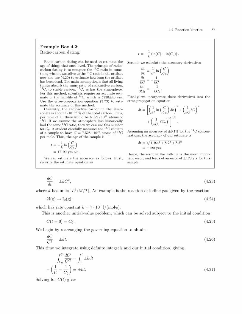
4.2 Reaction kinetics 87
Example Box 4.2:Radio-carbon dating.
Radio-carbon dating can be used to estimate theage of things that once lived. The principle of radio-carbon dating is to compare the 14C ratio in some-thing when it was alive to the 14C ratio in the artifactnow and use (4.20) to estimate how long the artifacthas been dead. The main assumption is that all livingthings absorb the same ratio of radioactive carbon,14C, to stable carbon, 12C, as has the atmosphere.For this method, scientists require an accurate esti-mate of the half-life of 14C, which is 5730±40 yrs.Use the error-propogation equation (3.73) to esti-mate the accuracy of this method.
Currently, the radioactive carbon in the atmo-sphere is about 1 ·10−10 % of the total carbon. Thus,per mole of C, there would be 6.022 · 1011 atoms of14C. If we assume the atmosphere has historicallyhad the same 14C ratio, then we can use this numberfor C0. A student carefully measures the 14C contentof a sample to have C = 7.528 · 1010 atoms of 14Cper mole. Thus, the age of the sample is
t = − 1
kln(
C
C0
)
= 17190 yrs old.
We can estimate the accuracy as follows. First,re-write the estimate equation as
t = − 1
k(ln(C) − ln(C0)) .
Second, we calculate the necessary derivatives
∂t
∂k=
1
k2ln(
C
C0
)
∂t
∂C= − 1
kC∂t
∂C0
= − 1
kC0
.
Finally, we incorporate these derivatives into theerror-propagation equation
δt =
[
(
1
k2ln(
C
C0
)
δk)2
+(
1
kCδC)2
+(
1
kC0
δC0
)2]1/2
.
Assuming an accuracy of ±0.1% for the 14C concen-trations, the accuracy of our estimate is
δt =√
119.42 + 8.22 + 8.32
= ±120 yrs.
Hence, the error in the half-life is the most impor-tant error, and leads of an error of ±120 yrs for thissample.
dC
dt= ±kC2, (4.23)
where k has units [L3/M/T ]. An example is the reaction of iodine gas given by the reaction
2I(g) → I2(g), (4.24)
which has rate constant k = 7 · 109 l/(mol·s).This is another initial-value problem, which can be solved subject to the initial condition
C(t = 0) = C0. (4.25)
We begin by rearranging the governing equation to obtain
dC
C2= ±kt. (4.26)
This time we integrate using definite integrals and our initial condition, giving∫ C
C0
dC ′
C ′2 =
∫ t
0±kdt
−(
1
C− 1
C0
)
= ±kt. (4.27)
Solving for C(t) gives

88 4. Physical, Chemical and Biological Transformations
0 0.2 0.4 0.6 0.8 1 1.2 1.4 1.6 1.8 20
0.2
0.4
0.6
0.8
1Solution for second−order reaction
Time
Con
cent
ratio
n
T1/2
Te
Fig. 4.2. Solution for a second-order transformation reaction. The reaction rate is k = −1.
C(t) =1
∓kt + 1/C0. (4.28)
Figure 4.2 plots this solution for decreasing concentration (positive sign in the equation) with
C0 = 1 and k = 1.
The characteristic times for a second-order reaction are given by
T1/2 = − 1
kC0, and (4.29)
Te = −(e − 1)
kC0. (4.30)
Hence, for second- and higher-order reactions, the characteristic times depend on the initial
concentration!
4.2.3 Higher-order reactions
The general equation for an nth-order reaction is
dC
dt= ±kCn, (4.31)
where k has units [L3(n−1)/M (n−1)/T ]. The general solution subject to the initial condition
C(t = 0) = C0 is(
1
(n − 1)
)
[
1
Cn−1− 1
C(n−1)0
]
= kt (4.32)
for n ≥ 2. Such reactions are rare, and one generally tries different values of n to find the best
fit to experimental data.
A common means of dealing with higher-order reaction rates is to linearize the reaction in
the vicinity of the concentration of interest, CI . The linearized reaction rate equation is
R = k∗C − kC2I , (4.33)

4.3 Incorporating transformation with the advective- diffusion equation 89
Jx,in Jx,out
x
-y
z
δxδy
δz
u
S
Fig. 4.3. Schematic of a control volume with crossflow and reaction.
where k is the real rate constant and k∗ is the linearized rate constant; note that kC2I is also a
constant. Thus, higher-order reactions can be treated as first-order reactions in the vicinity of a
known concentration CI .
4.3 Incorporating transformation with the advective-
diffusion equation
Having a thorough understanding of transformations and reaction kinetics, we are ready to
incorporate transformations into our transport equation, the advective diffusion equation. As we
pointed out earlier, reactions are treated differently, depending on whether they are homogeneous
or heterogeneous. Homogeneous reactions add a term to the governing differential equation;
whereas, heterogeneous reactions are enforced with special boundary conditions.
4.3.1 Homogeneous reactions: The advective-reacting
diffusion equation
Homogeneous reactions add a new term to the governing transport equation because they occur
everywhere within our system; hence, they provide another flux to our law of conservation of
mass. Referring to the control volume in Figure 4.3, the mass conservation equation is
∂M
∂t=∑
min −∑
mout ± S, (4.34)
where S is a source or sink reaction term. We have already seen in the derivation of the advective
diffusion equation that
δm =
(
D∂2C
∂x2i
− ui∂C
∂xi
)
δxδyδz. (4.35)

90 4. Physical, Chemical and Biological Transformations
Jn
δs
CV : δx δy δsZoom in
(Enlarge)
(a.) Macroscopic view of
surface reaction.
(b.) Microscopic view of
surface reaction.
x
z y
Fig. 4.4. Schematic representation of the reaction boundary condition. S represents the source or sink term, δs
is the reaction sublayer, and δxδy is the surface area into the page of the boundary control volume.
The reaction term is just the kinetic rate law integrated over the volume, giving
S = ±Rδxδyδz. (4.36)
Combining these results in an equation for the concentration, we obtain
∂C
∂t+
∂uiC
∂xi= D
∂2C
∂x2i
± R, (4.37)
where R has the same form as in the sections discussed above. Appendix B presents solutions
for a wide range of cases.
As an example, consider the solution for an instantaneous point source of a first-order reacting
substance in one dimension. The solution for C(t) can be found using Fourier transformation to
be
C(x, t) =M
A√
4πDtexp
(
−(x − ut)2
4Dt
)
exp(±kt), (4.38)
where M is the total mass of substance injected, A is the cross-sectional area, D is the diffusion
coefficient, u is the flow velocity, and k is the reaction rate constant. If we compare this solution
to the solution for a first-order reaction given in (4.20), we see that the initial concentration C0
is replaced by the time-varying solution in the absence of transformation. This observation is
helpful for deriving solutions to cases not presented in Appendix B.
4.3.2 Heterogeneous reactions: Reaction boundary conditions
Heterogeneous reactions occur only at the boundaries; hence, they provide new flux boundary
conditions as constraints on the governing transport equation. Examples include corrosion, where
there is an oxygen sink at the boundary, and also catalyst reactions, where the presence of other-
phase boundaries is needed to facilitate or speed up the reaction. Figure 4.4 shows a macroscopic
and microscopic view of the solid boundary. To define the boundary condition, we require an
expression for the source/sink flux, Jn.
Writing the conservation of mass for the control volume in the microscopic view, we have
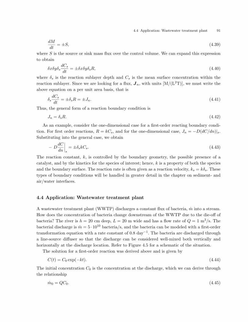
4.4 Application: Wastewater treatment plant 91
dM
dt= ±S, (4.39)
where S is the source or sink mass flux over the control volume. We can expand this expression
to obtain
δxδyδsdCs
dt= ±δxδyδsR, (4.40)
where δs is the reaction sublayer depth and Cs is the mean surface concentration within the
reaction sublayer. Since we are looking for a flux, Jn, with units [M/(L2T)], we must write the
above equation on a per unit area basis, that is
δsdCs
dt= ±δsR = ±Jn. (4.41)
Thus, the general form of a reaction boundary condition is
Jn = δsR. (4.42)
As an example, consider the one-dimensional case for a first-order reacting boundary condi-
tion. For first order reactions, R = kCs, and for the one-dimensional case, Jn = −D(dC/dn)|s.Substituting into the general case, we obtain
− DdC
dn
∣
∣
∣
∣
s= ±δskCs. (4.43)
The reaction constant, k, is controlled by the boundary geometry, the possible presence of a
catalyst, and by the kinetics for the species of interest; hence, k is a property of both the species
and the boundary surface. The reaction rate is often given as a reaction velocity, ks = kδs. These
types of boundary conditions will be handled in greater detail in the chapter on sediment- and
air/water interfaces.
4.4 Application: Wastewater treatment plant
A wastewater treatment plant (WWTP) discharges a constant flux of bacteria, m into a stream.
How does the concentration of bacteria change downstream of the WWTP due to the die-off of
bacteria? The river is h = 20 cm deep, L = 20 m wide and has a flow rate of Q = 1 m3/s. The
bacterial discharge is m = 5 ·1010 bacteria/s, and the bacteria can be modeled with a first-order
transformation equation with a rate constant of 0.8 day−1. The bacteria are discharged through
a line-source diffuser so that the discharge can be considered well-mixed both vertically and
horizontally at the discharge location. Refer to Figure 4.5 for a schematic of the situation.
The solution for a first-order reaction was derived above and is given by
C(t) = C0 exp(−kt). (4.44)
The initial concentration C0 is the concentration at the discharge, which we can derive through
the relationship
m0 = QC0. (4.45)
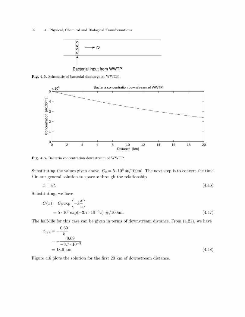
92 4. Physical, Chemical and Biological Transformations
Bacterial input from WWTP
Q
Fig. 4.5. Schematic of bacterial discharge at WWTP.
0 2 4 6 8 10 12 14 16 18 200
1
2
3
4
5x 10
6 Bacteria concentration downstream of WWTP
Distance [km]
Con
cent
ratio
n [#
/100
ml]
Fig. 4.6. Bacteria concentration downstream of WWTP.
Substituting the values given above, C0 = 5 · 106 #/100ml. The next step is to convert the time
t in our general solution to space x through the relationship
x = ut. (4.46)
Substituting, we have
C(x) = C0 exp
(
−kx
u
)
= 5 · 106 exp(−3.7 · 10−5x) #/100ml. (4.47)
The half-life for this case can be given in terms of downstream distance. From (4.21), we have
x1/2 = −0.69
k
= − 0.69
−3.7 · 10−5
= 18.6 km. (4.48)
Figure 4.6 plots the solution for the first 20 km of downstream distance.
Exercises 93
Summary
This chapter introduced the treatment of transformation processes. Three classes of transfor-
mations were considered: physical, chemical and biological. The rate laws governing the trans-
formations were derived from chemical reaction kinetics. Solutions for first and second order
reactions were derived, and methods for dealing with higher-order reactions and temperature
dependence of rate constants were presented. These rate laws were then combined with the
transport equation for two types of reactions: for homogeneous reactions, the rate law becomes
a source or sink term in the governing differential transport equation; for heterogeneous reac-
tions, a modified rate law becomes a boundary condition constraining the governing differential
equation. An example of bacterial die-off downstream of a WWTP closed the chapter.
Exercises
4.1 Reaction order. A chemical reaction is of order 1.5. What are the units of the rate constant?
What is the solution to the rate equation (i.e. what is C(t))? Write an expression for the half-life.
4.2 Clean disposal. A chemical tanker runs aground near the shore of a wide river. The company
declares the load on the tanker a complete loss, due to contamination by river water, and decides
to slowly discharge the hazardous material into the river to dispose of it. The material (an
industrial acid) reacts with the river water (the material is buffered by the river alkalinity)
and is converted to harmless products with a rate constant of k = 5 · 10−5 s−1. Calculate the
maximum discharge rate such that a concentration standard of 0.01 mg/l is not exceeded at a
distance of 1.5 km downstream. The river flow rate is Q = 15 m3/s, the depth is h = 2 m, the
width is B = 75 m, and the concentration of acid in the grounded tanker is 1200 mg/l. If the
tanker contains 10000 m3, how long will it take to safely empty the tanker?
4.3 Water treatment. In part of a water treatment plant, a mixing tank is used to remove
heavy metals. Untreated water flows into the tank where is it rigorously mixed (instantaneously
mixed) and brought into contact with other chemicals that remove the metals. A single outlet
is installed in the tank. Assume the inflow and outflow rates are identical, and assume metals
are removed in a first-order reaction with a rate constant of k = 0.06 s−1. The tank volume is
15 m3. What is the allowable flow rate such that the exit stream contains 10% of the metals in
the input stream? How high can the flow rate be if the reaction rate constant is doubled?

94 4. Physical, Chemical and Biological Transformations
5. Boundary Exchange: Air-Water and
Sediment-Water Interfaces
In the previous chapter we introduced transformation and described both homogeneous and
heterogeneous reactions. Now, we would like to look in more detail at heterogeneous reactions
and discuss the chemical and physical processes at interfaces that lead to boundary fluxes of
chemical species. The two major boundary types in environmental fluid mechanics are the air-
water and sediment-water interfaces. Because the processes at both boundaries are very similar,
we treat them together in this chapter under the heading of boundary exchange.
This chapter is divided into three main sections. First, the boundary layer in the vicinity
of the interface is described, and two common models for treating the boundary dynamics are
introduced without specifying what type of boundary is involved. Second, the air-water interface
is introduced, and methods are described for treating gas exchange across the interface. As an
example, the Streeter-Phelps equation for predicting oxygen concentrations downstream of an
organic waste stream is introduced. Third, the sediment-water interface is described, including
the complex physical and transformation processes that bring sediment and water into contact,
and a short description of the chemistry that occurs at the sediment-water interface is provided.
5.1 Boundary exchange
Under the concept of boundary exchange, we are primarily interested in the transfer of substances
that can be dissolved in the water phase. Examples at the air-water interface include chemicals
present in both phases (the air and the water), such as oxygen and carbon dioxide, as well as
volatile chemicals that off-gas from the water into the atmosphere, where the concentration is
negligible, such as mercuric compounds (e.g. (CH3)2Hg), chlorinated hydrocarbons (e.g. CH2Cl),
and a host of other organic compounds. Examples at the sediment-water interface include metals,
salts, nutrients, and organic compounds.
The transfer of these substances at an interface leads to a net mass flux, J , which can
have diffusive and advective components. Diffusive transfer is often assumed to be controlled by
equilibrium chemistry. Advective transfer results from a host of processes, such as the ejection
of sea spray from waves or the flow of groundwater. In general, this net mass flux becomes a
boundary condition that is imposed on the governing transport equation that is then solved
either numerically or analytically.
The challenge in describing boundary exchange is in predicting the magnitude of J . Unfor-
tunately, the dynamics that control the magnitude of the exchange flux are often microscopic in
nature and must be predicted by sub-models. If we consider the example of sugar dissolving in a
Copyright c© 2004 by Scott A. Socolofsky and Gerhard H. Jirka. All rights reserved.
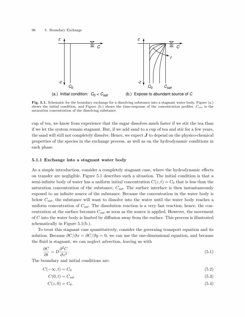
96 5. Boundary Exchange
-z
z
C
(a.) Initial condition: C0 < Csat
C0
-z
z
C
(b.) Expose to abundant source of C
C0 Csat
t
Fig. 5.1. Schematic for the boundary exchange for a dissolving substance into a stagnant water body. Figure (a.)shows the initial condition, and Figure (b.) shows the time-response of the concentration profiles. Csat is thesaturation concentration of the dissolving substance.
cup of tea, we know from experience that the sugar dissolves much faster if we stir the tea than
if we let the system remain stagnant. But, if we add sand to a cup of tea and stir for a few years,
the sand will still not completely dissolve. Hence, we expect J to depend on the physico-chemical
properties of the species in the exchange process, as well as on the hydrodynamic conditions in
each phase.
5.1.1 Exchange into a stagnant water body
As a simple introduction, consider a completely stagnant case, where the hydrodynamic effects
on transfer are negligible. Figure 5.1 describes such a situation. The initial condition is that a
semi-infinite body of water has a uniform initial concentration C(z, t) = C0 that is less than the
saturation concentration of the substance, Csat. The surface interface is then instantaneously
exposed to an infinite source of the substance. Because the concentration in the water body is
below Csat, the substance will want to dissolve into the water until the water body reaches a
uniform concentration of Csat. The dissolution reaction is a very fast reaction; hence, the con-
centration at the surface becomes Csat as soon as the source is applied. However, the movement
of C into the water body is limited by diffusion away from the surface. This process is illustrated
schematically in Figure 5.1(b.).
To treat this stagnant case quantitatively, consider the governing transport equation and its
solution. Because ∂C/∂x = ∂C/∂y = 0, we can use the one-dimensional equation, and because
the fluid is stagnant, we can neglect advection, leaving us with
∂C
∂t= D
∂2C
∂z2. (5.1)
The boundary and initial conditions are:
C(−∞, t) = C0 (5.2)
C(0, t) = Csat (5.3)
C(z, 0) = C0. (5.4)
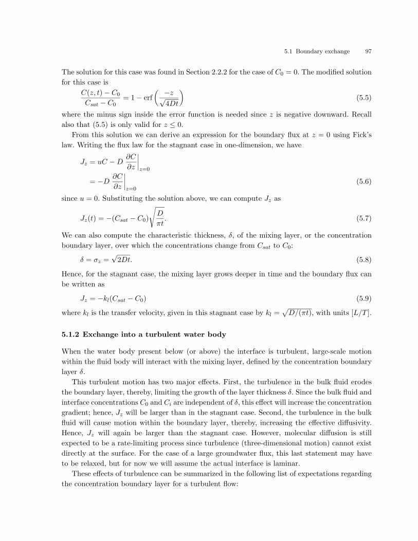
5.1 Boundary exchange 97
The solution for this case was found in Section 2.2.2 for the case of C0 = 0. The modified solution
for this case is
C(z, t) − C0
Csat − C0= 1 − erf
( −z√4Dt
)
(5.5)
where the minus sign inside the error function is needed since z is negative downward. Recall
also that (5.5) is only valid for z ≤ 0.
From this solution we can derive an expression for the boundary flux at z = 0 using Fick’s
law. Writing the flux law for the stagnant case in one-dimension, we have
Jz = uC − D∂C
∂z
∣
∣
∣
∣
z=0
= −D∂C
∂z
∣
∣
∣
∣
z=0(5.6)
since u = 0. Substituting the solution above, we can compute Jz as
Jz(t) = −(Csat − C0)
√
D
πt. (5.7)
We can also compute the characteristic thickness, δ, of the mixing layer, or the concentration
boundary layer, over which the concentrations change from Csat to C0:
δ = σz =√
2Dt. (5.8)
Hence, for the stagnant case, the mixing layer grows deeper in time and the boundary flux can
be written as
Jz = −kl(Csat − C0) (5.9)
where kl is the transfer velocity, given in this stagnant case by kl =√
D/(πt), with units [L/T ].
5.1.2 Exchange into a turbulent water body
When the water body present below (or above) the interface is turbulent, large-scale motion
within the fluid body will interact with the mixing layer, defined by the concentration boundary
layer δ.
This turbulent motion has two major effects. First, the turbulence in the bulk fluid erodes
the boundary layer, thereby, limiting the growth of the layer thickness δ. Since the bulk fluid and
interface concentrations C0 and Ci are independent of δ, this effect will increase the concentration
gradient; hence, Jz will be larger than in the stagnant case. Second, the turbulence in the bulk
fluid will cause motion within the boundary layer, thereby, increasing the effective diffusivity.
Hence, Jz will again be larger than the stagnant case. However, molecular diffusion is still
expected to be a rate-limiting process since turbulence (three-dimensional motion) cannot exist
directly at the surface. For the case of a large groundwater flux, this last statement may have
to be relaxed, but for now we will assume the actual interface is laminar.
These effects of turbulence can be summarized in the following list of expectations regarding
the concentration boundary layer for a turbulent flow:
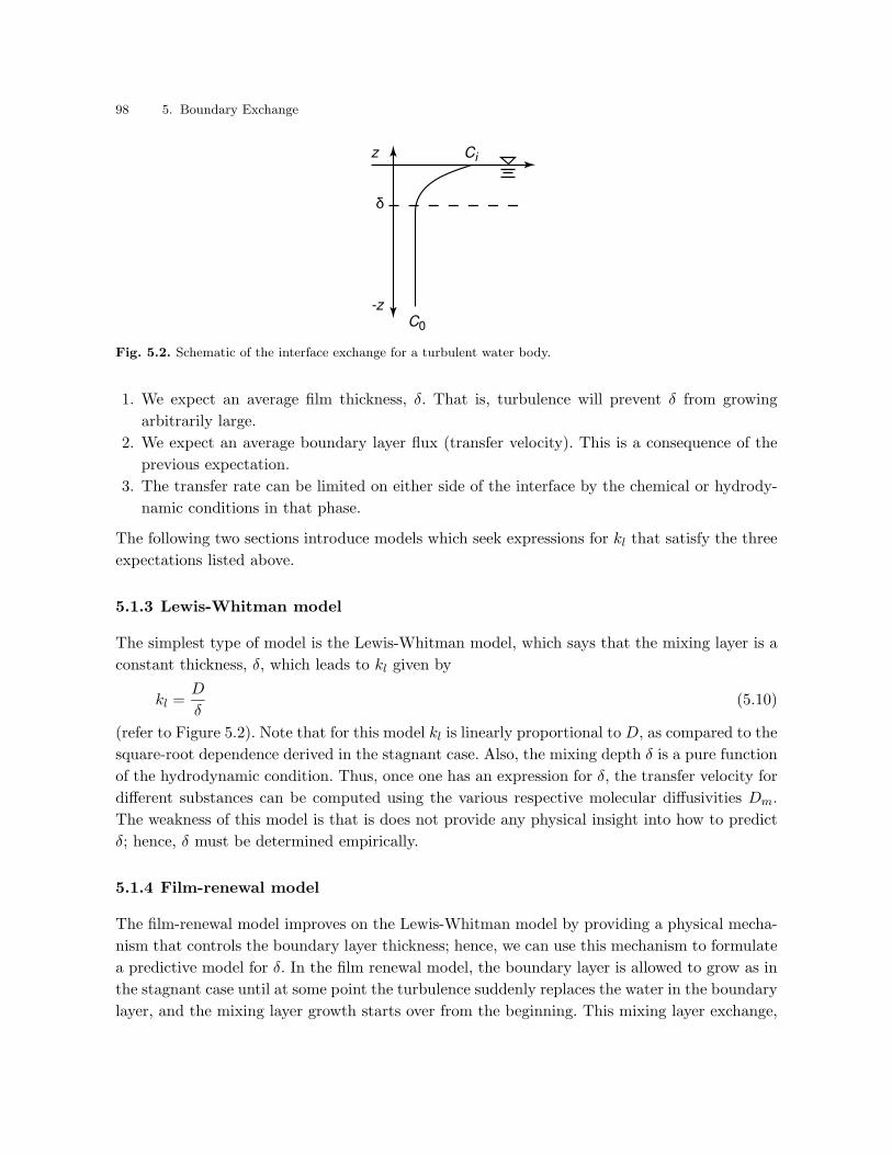
98 5. Boundary Exchange
-z
z
C0
δ
Ci
Fig. 5.2. Schematic of the interface exchange for a turbulent water body.
1. We expect an average film thickness, δ. That is, turbulence will prevent δ from growing
arbitrarily large.
2. We expect an average boundary layer flux (transfer velocity). This is a consequence of the
previous expectation.
3. The transfer rate can be limited on either side of the interface by the chemical or hydrody-
namic conditions in that phase.
The following two sections introduce models which seek expressions for kl that satisfy the three
expectations listed above.
5.1.3 Lewis-Whitman model
The simplest type of model is the Lewis-Whitman model, which says that the mixing layer is a
constant thickness, δ, which leads to kl given by
kl =D
δ(5.10)
(refer to Figure 5.2). Note that for this model kl is linearly proportional to D, as compared to the
square-root dependence derived in the stagnant case. Also, the mixing depth δ is a pure function
of the hydrodynamic condition. Thus, once one has an expression for δ, the transfer velocity for
different substances can be computed using the various respective molecular diffusivities Dm.
The weakness of this model is that is does not provide any physical insight into how to predict
δ; hence, δ must be determined empirically.
5.1.4 Film-renewal model
The film-renewal model improves on the Lewis-Whitman model by providing a physical mecha-
nism that controls the boundary layer thickness; hence, we can use this mechanism to formulate
a predictive model for δ. In the film renewal model, the boundary layer is allowed to grow as in
the stagnant case until at some point the turbulence suddenly replaces the water in the boundary
layer, and the mixing layer growth starts over from the beginning. This mixing layer exchange,
5.1 Boundary exchange 99
or film-renewal, occurs periodically with a renewal frequency that is a function of the turbulent
characteristics of the flow.
Under the idealized case that the boundary layer grows undisturbed until it is suddenly
completely replaced by water from the bulk turbulent flow, the net flux at the boundary can
be determined analytically. The governing transport equation and the initial and boundary
conditions are exactly the same as in the stagnant case (see (5.1) to (5.4)). The solution is given
by (5.5), and the net flux at the boundary is given by (5.7). These solutions are only valid,
however, from t = 0 to t = tr, the time between renewal events. The mean boundary flux over
one cycle can be found easily by taking the time average
Jz =1
tr
∫ t+tr
tJz(t)dt
=1
tr
∫ t+tr
t−(Ci − C0)
√
D
πtdt
= −(Ci − C0)
√
4D
πtr(5.11)
or, since the renewal frequency, r, is just 1/tr,
Jz = −(Ci − C0)
√
4Dr
π. (5.12)
Thus, the average transfer velocity is independent of time and is given by
kl =
√
4Dr
π(5.13)
which leaves us with the need to predict r.
The renewal frequency r is a characteristic of the turbulence. Recall that a turbulent flow is
a spectrum of eddy sizes, from the integral scale down to the Kolmogorov scale, and is driven,
for homogeneous turbulence, by the dissipation rate
ε =u3
I
lI(5.14)
where uI and lI are the integral velocity and length scales of the flow, respectively. For a shear
flow, the approximations uI = u∗ and lI = h are generally valid, where u∗ is the shear velocity
and h is the depth of the shear layer. We can derive two extreme estimates for r: one for the
case that the concentration boundary layer is renewed by Kolmogorov-scale eddies (called the
small-eddy estimate), and another for the case that the concentration boundary layer is renewed
by integral-scale eddies (called the large-eddy estimate).
Small-eddy estimate of r. Since the smallest eddies are dissipated by viscosity ν, an estimate
for the Kolmogorov time scale tK can be written as
tK =
√
ν
ε. (5.15)
Taking r as 1/tK and substituting approximations for uI and lI for a shear flow, we can obtain

100 5. Boundary Exchange
r =
√
u3∗
hν. (5.16)
If we further substitute the shear velocity as u∗ = u√
f/8, where u is the mean flow velocity
and f is a friction coefficient, then an estimate for kl can be written as
kl = Ku3/4
h1/4(5.17)
where K is a constant that depends on the fluid properties (i.e. ν) , the physico-chemical
properties of the substance (i.e. D), and on the boundary type (i.e. f). For kl at the air-water
interface with units cm/s, K is of order 10−1 to 100.
Large-eddy estimate of r. The time scale of the largest eddies is given by the integral time
scale tI , which for a shear flow is
tI =u∗h
. (5.18)
Taking r = 1/tI , and substituting u∗ = u√
f/8 leads the the expression for kl given by
kl = Ku1/2
h1/2(5.19)
where K is another constant which depends on the the physico-chemical properties of the sub-
stance (i.e. D), and on the boundary type (i.e. f).
Experimental data are sparse, but tend to agree better with the relationship kl ∝ u3/4; hence,
it is most likely the small-scale eddies that are responsible for the film renewal.
5.2 Air/water interface
At the air-water interface we are primarily concerned with the transfer of gases that can be
dissolved in the water. The substance may, or may not, be measurable in the gas phase. Figure 5.3
demonstrates the general case for a substance with measurable concentrations in both the gas and
liquid phase. As the figure demonstrates, there is a concentration boundary layer in the vicinity
of the water surface for both the phases. Because there cannot be a build-up of concentration
at the interface, the flux from the gas into the water, ma, must equal the flux at the interface
into the water, mw. Hence, only one of the phases contains the rate-limiting step.
The rate of transfer at the interface is controlled by the transfer velocity kl; thus, the rate-
limiting phase will have the lowest value of kl. Consider first the Lewis-Whitman model. The
transfer velocity increases as the diffusion coefficient increases and as the concentration boundary
layer gets thinner. Both of these conditions are higher in the gas phase than in the liquid phase.
The more complex film-renewal model gives the same conclusion: the flux at the interface can be
higher in the air than in the water. Therefore, we generally assume the substance is immediately
available at the gas side of the interface, and we must only consider the concentration boundary
layer in the water phase in order to compute the net flux at the boundary.
Because the air-water interface is a moving boundary, two further complications can arise
that are not addressed in either of our boundary transfer models. First, wind generates shear
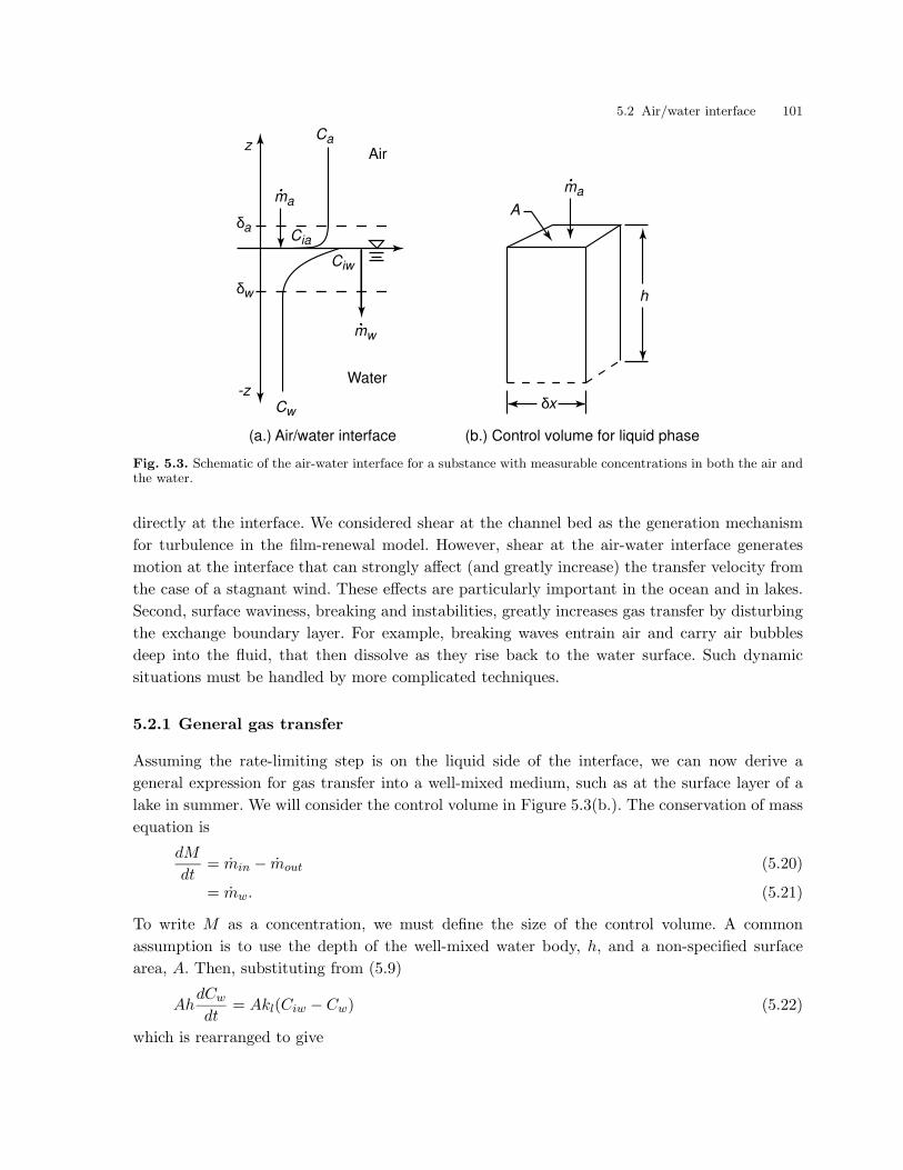
5.2 Air/water interface 101
-z
z
Cw
δw
δa
Ciw
Cia
Ca
ma
mw
Air
Water
ma
h
δx
A
(a.) Air/water interface (b.) Control volume for liquid phase
Fig. 5.3. Schematic of the air-water interface for a substance with measurable concentrations in both the air andthe water.
directly at the interface. We considered shear at the channel bed as the generation mechanism
for turbulence in the film-renewal model. However, shear at the air-water interface generates
motion at the interface that can strongly affect (and greatly increase) the transfer velocity from
the case of a stagnant wind. These effects are particularly important in the ocean and in lakes.
Second, surface waviness, breaking and instabilities, greatly increases gas transfer by disturbing
the exchange boundary layer. For example, breaking waves entrain air and carry air bubbles
deep into the fluid, that then dissolve as they rise back to the water surface. Such dynamic
situations must be handled by more complicated techniques.
5.2.1 General gas transfer
Assuming the rate-limiting step is on the liquid side of the interface, we can now derive a
general expression for gas transfer into a well-mixed medium, such as at the surface layer of a
lake in summer. We will consider the control volume in Figure 5.3(b.). The conservation of mass
equation is
dM
dt= min − mout (5.20)
= mw. (5.21)
To write M as a concentration, we must define the size of the control volume. A common
assumption is to use the depth of the well-mixed water body, h, and a non-specified surface
area, A. Then, substituting from (5.9)
AhdCw
dt= Akl(Ciw − Cw) (5.22)
which is rearranged to give
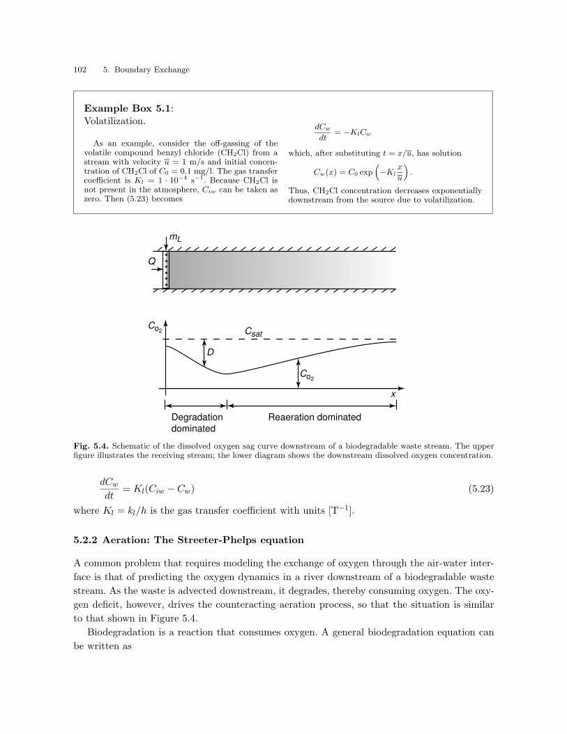
102 5. Boundary Exchange
Example Box 5.1:Volatilization.
As an example, consider the off-gassing of thevolatile compound benzyl chloride (CH2Cl) from astream with velocity u = 1 m/s and initial concen-tration of CH2Cl of C0 = 0.1 mg/l. The gas transfercoefficient is Kl = 1 · 10−4 s−1. Because CH2Cl isnot present in the atmosphere, Ciw can be taken aszero. Then (5.23) becomes
dCw
dt= −KlCw
which, after substituting t = x/u, has solution
Cw(x) = C0 exp(
−Klx
u
)
.
Thus, CH2Cl concentration decreases exponentiallydownstream from the source due to volatilization.
x
Co2
D
Co2
Degradation
dominated
Reaeration dominated
Csat
Q
mL
Fig. 5.4. Schematic of the dissolved oxygen sag curve downstream of a biodegradable waste stream. The upperfigure illustrates the receiving stream; the lower diagram shows the downstream dissolved oxygen concentration.
dCw
dt= Kl(Ciw − Cw) (5.23)
where Kl = kl/h is the gas transfer coefficient with units [T−1].
5.2.2 Aeration: The Streeter-Phelps equation
A common problem that requires modeling the exchange of oxygen through the air-water inter-
face is that of predicting the oxygen dynamics in a river downstream of a biodegradable waste
stream. As the waste is advected downstream, it degrades, thereby consuming oxygen. The oxy-
gen deficit, however, drives the counteracting aeration process, so that the situation is similar
to that shown in Figure 5.4.
Biodegradation is a reaction that consumes oxygen. A general biodegradation equation can
be written as

5.2 Air/water interface 103
OM + O2 → CO2 + H2O + new cells + stable productsmicroorganisms
where OM stands for organic matter (the biodegradable waste). It can be shown in the laboratory
that the consumption of OM is a first-order reaction. Thus, the rate-law for the consumption of
OM is given by
d[OM]
dt= −kd[OM] (5.24)
where kd is the rate constant for biodegradation. In the classical literature on this subject, the
concentration of OM is called the oxygen demand and is given the symbol L. Substituting L for
[OM] in the above equation and imposing the initial condition L(t = 0) = L0, the solution for
the consumption of oxygen demand becomes
L(t) = L0 exp(−kdt) (5.25)
where L0 is called the ultimate carbonaceous oxygen demand. The word carbonaceous refers to
the fact that the oxygen consumption is due to conversion of carbon-based organic matter as
opposed to any other chemical reaction that might consume oxygen. Because O2 is consumed
at the same rate as OM, we can write the following relationship:
d[O2]
dt=
d[OM]
dt= −kdL0 exp(−kdt). (5.26)
If we define the oxygen deficit, D = ([O2]sat − [O2]), then the production of oxygen deficit is
given by
dD
dt= kdL0 exp(−kdt). (5.27)
This equation represents a sink term for oxygen due to biodegradation of the waste stream.
At the same time the waste is being degraded the river is being aerated by exchange at the
air-water interface. The mass flux of oxygen, mO2, is derived from the boundary exchange flux
in (5.9)
mO2= −Akr([O2]sat − [O2])
= −AkrD (5.28)
where kr is the river aeration transfer velocity for oxygen and the negative sign indicates a flux
of oxygen goes into the river.
We can now use the control volume in Figure 5.3(b.) to derive the oxygen balance downstream
of the waste source. If we make the one-dimensional assumption and move our control volume
with the mean flow velocity in the river, then the mass balance for our control volume is
dMO2
dt= mO2
− S (5.29)
where S is a sink term representing the biodegradation process. Taking the width of the river as
W and the depth as h, we can write the equation for the concentration of O2 as

104 5. Boundary Exchange
Wδxhd[O2]
dt= mO2
− S
= Wδxkr([O2]sat − [O2]) − WδxhRO2(5.30)
where RO2is the reaction rate law for the consumption of O2. Rewriting this equation for the
oxygen deficit D, we have
dD
dt= RD − KrD (5.31)
where RD is the rate law for the production of D and Kr = kr/h is the oxygen transfer coefficient.
Substituting (5.27) RD, we obtain the inhomogeneous ordinary differential equation
dD
dt= kdL0 exp(−kdt) − KrD (5.32)
subject to the initial condition D(t = 0) = D0, which is the initial oxygen deficit just upstream
of the point where the waste stream is introduced. The solution to this equation is the classic
Streeter-Phelps equation:
D(t) =kdL0
Kr − kd(exp(−kdt) − exp(−Krt)) + D0 exp(−Krt). (5.33)
The derivation of this solution is given in Appendix C.
5.3 Sediment/water interface
Unlike the air-water interface, where the interface is generally confined to an abrupt transition
at the water surface, the sediment-water interface is very difficult to define and is controlled by a
number of complicated physical and chemical processes. The real difficulty of the sediment-water
interface lies in the multi-phase (dispersive) nature of the interface. At an individual sediment
grain, the interface may be clearly defined. However, since we cannot treat every sediment grain
individually, a continuum description of the system is necessary. Two important quantities are
used to describe dispersed systems. The porosity, n, is the volume of water contained in a unit
volume of mixture
n =Vw
V. (5.34)
This parameter can vary widely, but is generally between 0.1 and 0.9 within a porous media
(groundwater system) and is 0.99 and higher within the water column (suspended sediment
system). For suspended sediments, the second parameter is also important: the slip velocity, or
settling velocity, us. The settling velocity is generally taken as the terminal fall velocity of the
sediment in a quiescent system. The porous media/water column interface can then be defined
as the point where n becomes small enough that us goes to zero due to contact with other
sediment particles, forming a (relatively) fixed matrix.
As shown in Figure 5.5 many processes lead to the transport of chemical species in the water
column and through the sediment bed. These processes are organized in the figure into two
categories. On the left are physical processes that do not involve chemical transformation; on
the right are chemical and biological processes.

5.3 Sediment/water interface 105
Example Box 5.2:Dissolved-oxygen sag curve.
As an example of the application of the Streeter-Phelps equation, consider the following wastestream. A wastewater treatment plant dischargesan oxygen demanding waste stream at a rate ofm = 295 g/s of BOD (biochemical oxygen demand)into a stream h = 3 m deep, W = 30 m wide, andwith a flow rate Q = 27 m3/s. The waste streamis introduced through a longitudinal diffuser so thatthe we can assume complete lateral and vertical mix-ing at the source. The initial concentration of BODin the river L0 is then
L0 =m
Q
=295
27= 10.9 mg/l.
Based on regular experiments conducted by the fa-cility operator, the decay rate of the waste is knownto be kd = 0.2 day−1.
A rule of thumb often used for computing the aer-ation rate is
Kr =3.9u1/2
h3/2
where Kr is in day−1, u is the mean stream ve-locity in m/s, and h is the depth in m. For thisstream Kr = 0.4 day−1. The initial oxygen deficitwas measured to be D0 = 1.5 mg/l (the saturationoxygen concentration is 9.1 mg/l). The plot belowshows the solution (5.33) for the oxygen concentra-tion ([O2]sat − D) downstream of the mixing zone.The critical time to reach the minimum oxygen con-centration is
tc =1
Kr − kdln
[
Kr
kd
(
1 − D0(Kr − kd)
kdL0
)]
which for this case is 2.67 days, or 69 km. This exam-ple illustrates how slow the aeration process can bein the absence of aeration devices, such as cascadesand water falls.
0 50 100 150 200 250 3006
6.5
7
7.5
8
8.5Dissolved oxygen concentration downstream of pollutant discharge
[O2] i
n m
g/l
Distance [km]
The physical processes are responsible for transport. Within the water column, chemicals can
move with either the solid or liquid phase. Of the transport processes listed in the figure, we
have already discussed advection and diffusion (both turbulent and molecular) in detail. The
other transport processes in the water column (which are specific to the sediment phase) are:
• Flocculation and settling: flocculation is the sticking together of several sediment particles
to form larger particles. Settling is the downward fall of sediment particles due to their negative
buoyancy. Accept for very small particles (colloids), sediment particles always have a negative
vertical velocity component relative to the water column motion.
• Sedimentation: sedimentation is the process whereby sediment is lost from the water column
and gained by the sediment bed. This occurs once the settling sediment particles reach the
channel, lake or ocean bottom and rejoin the sediment bed.

106 5. Boundary Exchange
- Advection
- Diffusion (turbulent/molecular)
- Flocculation/Settling
Sedimentation Erosion
- Ad-/Desorption
- Chemical reactions
- Biological reactions
- Bioturbation
- Advection in porous media
- Diffusion/Dispersion in porous
media
Groundwater advective flux
- Ad-/Desorption
- Chemical reactions
- Biological reactions
Active
layer
Immoble
layer
Wa
ter
co
lum
nP
oro
us m
ed
ia
Physical/Mechanics processes Chemical/Biological
processes
u(z)Csed (z)
Fig. 5.5. Schematic of processes occurring at the sediment-water interface, in the water column and in thesediment bed (porous media).
• Erosion: erosion is the process by which sediment is lost from the sediment bed and entrained
into the water column.
Within the sediment bed, or porous media, further transport processes are at work. For species
in the liquid phase, the processes of advection, diffusion, and dispersion are active throughout
the porous media. For the sediment particles, physical transport occurs only in the upper active
layer due to the process of bioturbation:
• Bioturbation: bioturbation is the name given to the mixing of sediment caused by animals
living in the sediment (mostly worms). These animals move sediment as they dig. Two impor-
tant classes of worms mix the sediment differently. In the one case, sediment is eaten at the
base of the active layer and moved up to the surface. In the other case, sediment is removed
from the surface and carried down to the bottom of the active layer. The net movement of sed-
iment is often modeled by an enhanced diffusion process, where we use bioturbation diffusion
coefficients.
Through the combination of all these transport processes, chemical species move in and out of
the water column and the porous media.
Through transformation processes, chemical species move in and out of the solid and liquid
phases and, also, change to other species. We have already discussed chemical and biological
transformation reactions. These reactions occur both in the water column and in the porous
media. They can also occur in either the liquid phase, the solid phase or at the interface.
5.3 Sediment/water interface 107
Processes at the sediment interface are particularly important for the transport of chemicals
through these multi-phase systems:
• Adsorption/desorption: the chemical processes of adsorption and desorption control the
distribution of certain chemicals between the solid and liquid phases. Due to complex chem-
ical/physical processes, some molecules have an affinity for sticking to the solid phase (often
due to electrical charge interaction). That is, some molecules would rather stick to a sedi-
ment particle than remain dissolved in the surrounding fluid. The behavior of most organic
compounds and heavy metals is controlled by sorption chemistry.
Because sorption is a dominant process occurring at the sediment-water interface, it is discussed
in more detail at the end of this section.
As discussed in Gschwend (1987), the processes at the sediment-water interface (at the bottom
of a lake or channel) depend on the energetic state of the water body. Beginning with laminar
conditions (as in a deep lake) and progressing to increasingly energetic, turbulent conditions (as
in reservoirs, estuaries, and streams), the progression is as follows. With no motion, exchange
occurs due to direct sorption exchange and diffusion of dissolved species from the pore water.
Next, the system begins to flow, allowing the advective and dispersive flux of groundwater flow.
Bioturbation, which may always be present, adds energy by actively mixing the sediments. As
the water column begins to flow, sediments can be pushed along the top layer of sediments
in a process called bed-load transport. Finally, with an energetic water column, erosion begins,
sediment is carried up into the water column, and suspended transport (advection of sediment in
the water column) becomes important. Hence, the transport of species associated with sediment
is a complex problem dependent on the chemistry of the species and the mobility of the sediment.
5.3.1 Adsorption/desorption in disperse aqueous systems
Ignoring the complex problems that lead to the transport of sediment, we focus in this section
on the exchange at the solid/liquid interface of a mixed solution of suspended sediment particles
in a dispersed (large n) system. An important process controlling the distribution of many
toxins in sediment-laden solutions is adsorption/desorption. Defined above, this process causes
a large fraction of the sorbing compound to attach to the sediment particles. Hence, sorption
controls the concentration of dissolved contaminant, and causes much of the contaminant to be
transported with the sediment.
Figure 5.6 illustrates the situation. Sorbing compounds include most polar and non-polar
organic compounds and heavy metal ions. To describe the situation quantitatively, we define two
concentrations. First, the concentration of substance A that is dissolved in solution is designated
C and is defined as
C =Mdissolved
Vw(5.35)
having normal concentration units. Second, the non-dimensional sorbed-fraction concentration,
C∗s , is defined as

108 5. Boundary Exchange
Solid Liquid
Adsorption
Desorption
AA
Fig. 5.6. Schematic of the adsorption/desorption process for the molecule A.
C∗s =
Madsorbed/Vw
Msediment/Vw
=Madsorbed
Msediment. (5.36)
These equations are valid only for highly dispersed systems, where nV ≈ V .
Because sorption kinetics are very fast, we can usually assume that equilibrium exists be-
tween the adsorbed and desorbed fractions. Based on experiments, the following simple type of
equilibrium relationship has been proposed:
C∗s =
ΓC
K + C(5.37)
which is called the Langmuir equation. The coefficient K is a constant with units of concen-
tration; the coefficient Γ is a non-dimensional constant, called the Langmuir isotherm, which
gives the asymptotic value of C∗s as C becomes large. Figure 5.7 plots the Langmuir equation
for Γ = 1 and K = 1. For most toxins in the environment, C K, and we can simplify the
Langmuir equation to
C∗s = PC (5.38)
where P is the partition coefficient with units [L3/M]. Typical values of P are between 103 to
106 l/kg.
In order to avoid the confusion caused by C∗s being non-dimensional, a dimensional concen-
tration of adsorbed contaminant is convenient to define. From the density of the sediment ρs
and the porosity, the dimensional adsorbed concentration is
Cs = C∗s ρs
(
1 − n
n
)
= KDC (5.39)
where KD is a non-dimensional distribution coefficient. It is important to note that P is a
purely physico-chemical parameter; whereas, KD also depends on the sediment concentration
and physical characteristics (through the porosity and density, respectively).
Summary
This chapter introduced the processes that result in boundary exchange of chemical species. The
general issue in describing boundary exchange is in determining the net boundary flux J . Once

5.3 Sediment/water interface 109
0 1 2 3 4 5 6 7 8 9 100
0.2
0.4
0.6
0.8
1
Langmuir equation for De−/Adsorption
Dissolved concentration [M/L3]
Sor
bed
conc
entr
atio
n [−
−]
K
Γ
Fig. 5.7. Langmuir equation for de-/adsorption with Γ = 1 and K = 1. Note that C∗
s is 1/2 at C = K.
Example Box 5.3:Naphthalene partitioning.
Consider the partitioning of the organic toxinnaphthalene, the smallest of the polynuclear aro-matic hydrocarbons (PAHs). We wish to find thefraction of dissolved to adsorbed naphthalene, fd.Using (5.38), this fraction is given by
fd =C
C + Cs
=1
1 + ρs
(
1−nn
)
P.
For naphthalene P = 103 l/kg. Typical sediment hasa density of 2600 kg/m3. For a mixture with n =0.99, fd = 4%.
We can see that fd is always large for low concen-trations C by looking at the range of expected KD.From above
KD = ρs
(
1 − n
n
)
P.
Making the following order-or-magnitude estimates
ρs = 103
(1 − n)/n = 10−3
P = 103 to 106
KD ranges from 103 to 106; fd ranges from 10−3 to10−6. Therefore, we can assume that a large fractionof the contaminant is present in the sorbed state.
If we manage to eliminate the source of a toxiccontaminant that is also sorbed to the sediments,then the sediment bed itself will start to release itssediment load into the water column water, creatinga new source (see Exercise 5.3). Unfortunately, be-cause fd is so large, the sediment load is large, andit takes a long time before the water column is freefrom this sediment source of the contaminant.
that flux is know, boundary exchange becomes a boundary condition on the governing transport
equation. The solution for J in a stagnant water body was used to develop two descriptions of
exchange in turbulent water bodies. The Lewis-Whitman model, the simplest model, assumes
the concentration boundary layer between phases has a constant depth. The film-renewal model
assumes that turbulence constantly refreshes the fluid in the concentration boundary layer, and
that the renewal rate derives from turbulent eddy characteristics. The exchange at the air-water
interface was discussed in more detail, with examples for volatile chemicals and oxygen aeration.
The sediment-water interface was described qualitatively, and the sorption chemistry at the
sediment water interface was described in more detail.
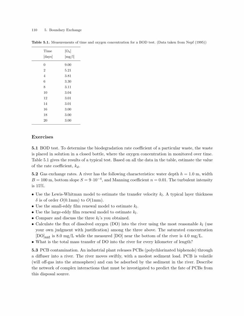
110 5. Boundary Exchange
Table 5.1. Measurements of time and oxygen concentration for a BOD test. (Data taken from Nepf (1995))
Time [O2]
[days] [mg/l]
0 9.00
2 5.21
4 3.81
6 3.30
8 3.11
10 3.04
12 3.01
14 3.01
16 3.00
18 3.00
20 3.00
Exercises
5.1 BOD test. To determine the biodegradation rate coefficient of a particular waste, the waste
is placed in solution in a closed bottle, where the oxygen concentration in monitored over time.
Table 5.1 gives the results of a typical test. Based on all the data in the table, estimate the value
of the rate coefficient, kd.
5.2 Gas exchange rates. A river has the following characteristics: water depth h = 1.0 m, width
B = 100 m, bottom slope S = 9·10−4, and Manning coefficient n = 0.01. The turbulent intensity
is 15%.
• Use the Lewis-Whitman model to estimate the transfer velocity kl. A typical layer thickness
δ is of order O(0.1mm) to O(1mm).
• Use the small-eddy film renewal model to estimate kl.
• Use the large-eddy film renewal model to estimate kl.
• Compare and discuss the three kl’s you obtained.
• Calculate the flux of dissolved oxygen (DO) into the river using the most reasonable kl (use
your own judgment with justification) among the three above. The saturated concentration
[DO]sat is 8.0 mg/L while the measured [DO] near the bottom of the river is 4.0 mg/L.
• What is the total mass transfer of DO into the river for every kilometer of length?
5.3 PCB contamination. An industrial plant releases PCBs (polychlorinated biphenols) through
a diffuser into a river. The river moves swiftly, with a modest sediment load. PCB is volatile
(will off-gas into the atmosphere) and can be adsorbed by the sediment in the river. Describe
the network of complex interactions that must be investigated to predict the fate of PCBs from
this disposal source.
Exercises 111
5.4 Sediment source of phosphorus. Phosphorus, in the form of phosphate (PO3−4 ), is often
a limiting nutrient for algae production in lakes. Because the uncontrolled growth of algae is
undesirable, the discharge of phosphorus into the environment should be minimized (this is why
you cannot buy laundry detergent any more that contains phosphorus). The U.S. Environmental
Protection Agency recommends a limit of 0.05 mg/l PO3−4 for streams that flow into freshwater
lakes.
An old chemical plant recently shut off their phosphorus discharge; however, high concentra-
tions of phosphorus are still being measured downstream of the chemical plant. After further
investigation, the following facts were collected:
• The concentration of phosphate in the stream water upstream of the plant is C0 = 0.003 mg/l.
• The sediments in the stream are saturated with sorbed phosphorus for a distance of 2 km
downstream of the plant.
• The phosphate concentration at the sediment bed is kept constant by desorption at a value of
Cb = 0.1 mg/l.
• The design conditions in the stream are h = 2 m deep and u = 0.2 m/s.
• The phosphate transfer velocity at the sediment bed is given approximately by the relationship
(film-renewal model):
kl = 0.002u3/4
h1/4in m/s. (5.40)
Based on the above data: What is the concentration of phosphate in the stream just after
passing the region of contaminated sediments? If the stream carries a suspended sediment load,
how would that affect the concentration of phosphate in the stream?

112 5. Boundary Exchange
6. Atmospheric Mixing
Previous chapters have dealt solely with transport in various water bodies and have presented
examples of one-dimensional solutions to the transport equations. We now turn our attention to
transport and mixing in the atmosphere, and by necessity, we will have to give more attention to
three-dimensional solutions. Because of the atmosphere’s unique composition and boundary and
forcing conditions, atmospheric turbulence is more complicated than the idealized homogeneous,
stationary, isotropic case. Moreover, these complications impact transport and mixing because
they determine the values of the turbulent diffusion and dispersion coefficients. Hence, a concise
discussion of atmospheric mixing requires also studying atmospheric turbulence and the resulting
modifications in the behaviour of mixing coefficients from the idealized case.
This chapter begins with an introduction to atmospheric turbulence and a review of turbu-
lent boundary layer structure. The log-velocity profile for a turbulent shear flow is introduced,
and the behaviour of turbulence throughout a neutrally stable atmospheric boundary layer is
described. Because of their importance to turbulence characteristics, the buoyancy effects of
heating and cooling within the boundary layer are discussed qualitatively. The discussion on
mixing begins with a review of turbulent mixing in three-dimensional, homogeneous, stationary
turbulence. The solution for a continuous point source is derived and used to illustrate mixing
in the remaining section. The chapter closes by adapting the idealized solution in homogeneous,
stationary turbulence to the turbulence present in the atmosphere.
Much of the material in this chapter was taken from Csanady (1973) and from Fedorovich
(1999). For further reading, those two sources are highly recommended, along with the classic
books by Lumley & Panofsky (1964) and Pasquill (1962) and more recent contributions by
Garratt (1992) and Kaimal & Finnigan (1994).
6.1 Atmospheric turbulence
In Environmental Fluid Mechanics, we are concerned with local mixing processes in fluids that
interact with living organisms. For the atmosphere, this means that we are interested in mixing
processes near the earth’s surface. Because of the no-slip boundary condition at the surface,
wind in the upper atmosphere generates a near-surface boundary layer, defined by variations in
velocity and often accompanied by variations in temperature (and density). Figure 6.1 shows
this situation schematically. Because of its dominant role in mixing near the earth’s surface, we
present here a short introduction to turbulence in the atmospheric boundary layer.
Copyright c© 2004 by Scott A. Socolofsky and Gerhard H. Jirka. All rights reserved.
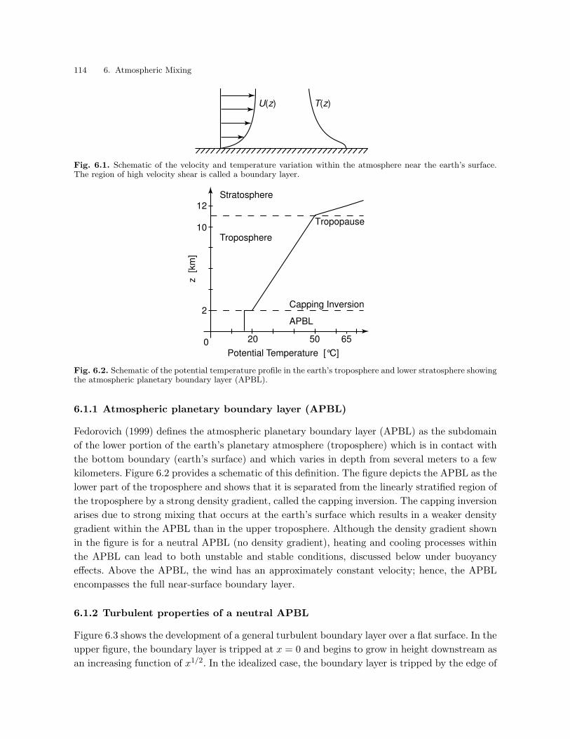
114 6. Atmospheric Mixing
U(z) T(z)
Fig. 6.1. Schematic of the velocity and temperature variation within the atmosphere near the earth’s surface.The region of high velocity shear is called a boundary layer.
APBL
Troposphere
Tropopause
z [k
m]
Capping Inversion
Potential Temperature [°C]0
2
10
12
20 50 65
Stratosphere
Fig. 6.2. Schematic of the potential temperature profile in the earth’s troposphere and lower stratosphere showingthe atmospheric planetary boundary layer (APBL).
6.1.1 Atmospheric planetary boundary layer (APBL)
Fedorovich (1999) defines the atmospheric planetary boundary layer (APBL) as the subdomain
of the lower portion of the earth’s planetary atmosphere (troposphere) which is in contact with
the bottom boundary (earth’s surface) and which varies in depth from several meters to a few
kilometers. Figure 6.2 provides a schematic of this definition. The figure depicts the APBL as the
lower part of the troposphere and shows that it is separated from the linearly stratified region of
the troposphere by a strong density gradient, called the capping inversion. The capping inversion
arises due to strong mixing that occurs at the earth’s surface which results in a weaker density
gradient within the APBL than in the upper troposphere. Although the density gradient shown
in the figure is for a neutral APBL (no density gradient), heating and cooling processes within
the APBL can lead to both unstable and stable conditions, discussed below under buoyancy
effects. Above the APBL, the wind has an approximately constant velocity; hence, the APBL
encompasses the full near-surface boundary layer.
6.1.2 Turbulent properties of a neutral APBL
Figure 6.3 shows the development of a general turbulent boundary layer over a flat surface. In the
upper figure, the boundary layer is tripped at x = 0 and begins to grow in height downstream as
an increasing function of x1/2. In the idealized case, the boundary layer is tripped by the edge of
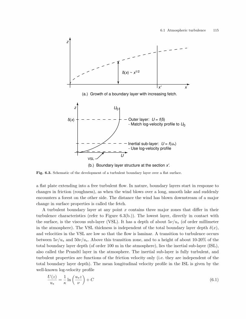
6.1 Atmospheric turbulence 115
Outer layer: U = f(δ)- Match log-velocity profile to U0
Inertial sub-layer: U = f(u*)
- Use log-velocity profile
U
z U0
VSL
δ(x)
δ(x) ~ x1/2
x' x
z
(a.) Growth of a boundary layer with increasing fetch.
(b.) Boundary layer structure at the section x'.
Fig. 6.3. Schematic of the development of a turbulent boundary layer over a flat surface.
a flat plate extending into a free turbulent flow. In nature, boundary layers start in response to
changes in friction (roughness), as when the wind blows over a long, smooth lake and suddenly
encounters a forest on the other side. The distance the wind has blown downstream of a major
change in surface properties is called the fetch.
A turbulent boundary layer at any point x contains three major zones that differ in their
turbulence characteristics (refer to Figure 6.3(b.)). The lowest layer, directly in contact with
the surface, is the viscous sub-layer (VSL). It has a depth of about 5ν/u∗ (of order millimeter
in the atmosphere). The VSL thickness is independent of the total boundary layer depth δ(x),
and velocities in the VSL are low so that the flow is laminar. A transition to turbulence occurs
between 5ν/u∗ and 50ν/u∗. Above this transition zone, and to a height of about 10-20% of the
total boundary layer depth (of order 100 m in the atmosphere), lies the inertial sub-layer (ISL),
also called the Prandtl layer in the atmosphere. The inertial sub-layer is fully turbulent, and
turbulent properties are functions of the friction velocity only (i.e. they are independent of the
total boundary layer depth). The mean longitudinal velocity profile in the ISL is given by the
well-known log-velocity profile
U(z)
u∗=
1
κln
(
u∗z
ν
)
+ C (6.1)

116 6. Atmospheric Mixing
where κ ≈ 0.4 is the von Karman constant and C is an integration constant about equal to five.
It is important to note that within this layer U(z) is independent of δ(x). The remaining region
of the boundary layer is called the outer layer, or Ekman layer in the atmosphere, and extends up
to where the velocity becomes U0. Within the atmosphere, the Ekman layer is deep enough that
it experiences Coriolis effects due to the earth’s rotation. In the outer layer, turbulence properties
and the velocity profile are dependent on the total layer depth, and we use a technique called
matching to adjust the log-velocity profile in this layer so that it reaches U0 at z = δ(x).
In general, turbulence measurements in the APBL depend on the height of the measurement,
the roughness of the ground, and the stability (Csanady 1973). Measurements near the surface
(within the ISL) demonstrate that
urms ∝ u∗ (6.2)
where urms = (u′2)1/2. Above this surface layer, urms tends to decay with height. Because the
land surface is quite rough in comparison to an idealized flat plate, the log-velocity profile cited
above is adjusted in the ISL to give
U(z) =u∗κ
ln
(
z
z0
)
(6.3)
where z0 is the roughness height (valid for z z0).
Because the mean wind-speed increases with height and the turbulent fluctuation velocities
are constant with height within the neutral APBL, turbulence intensity decreases with height.
Turbulence intensity is defined as
ix =(u′2)1/2
U(z)(6.4)
iy =(v′2)1/2
U(z)(6.5)
iz =(w′2)1/2
U(z)(6.6)
where iy and iz are the turbulence intensities (non-dimensional), u′ is the longitudinal fluctuation
velocity, v′ is the transverse fluctuation velocity, and w′ is the vertical fluctuation velocity.
Measurements by Panofsky (1967) revealed for a neutral surface layer that
(u′2)1/2 = 2.2u∗ (6.7)
(v′2)1/2 = 2.2u∗ (6.8)
(w′2)1/2 = 1.25u∗. (6.9)
Combining these relationships with the log velocity profile yields
ix = iy =0.88
ln(z/z0)(6.10)
iz =0.50
ln(z/z0). (6.11)
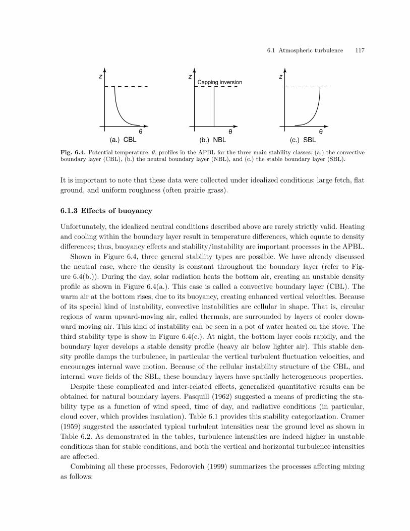
6.1 Atmospheric turbulence 117
θ
z
(a.) CBL
θ
z
(b.) NBL
θ
z
(c.) SBL
Capping inversion
Fig. 6.4. Potential temperature, θ, profiles in the APBL for the three main stability classes: (a.) the convectiveboundary layer (CBL), (b.) the neutral boundary layer (NBL), and (c.) the stable boundary layer (SBL).
It is important to note that these data were collected under idealized conditions: large fetch, flat
ground, and uniform roughness (often prairie grass).
6.1.3 Effects of buoyancy
Unfortunately, the idealized neutral conditions described above are rarely strictly valid. Heating
and cooling within the boundary layer result in temperature differences, which equate to density
differences; thus, buoyancy effects and stability/instability are important processes in the APBL.
Shown in Figure 6.4, three general stability types are possible. We have already discussed
the neutral case, where the density is constant throughout the boundary layer (refer to Fig-
ure 6.4(b.)). During the day, solar radiation heats the bottom air, creating an unstable density
profile as shown in Figure 6.4(a.). This case is called a convective boundary layer (CBL). The
warm air at the bottom rises, due to its buoyancy, creating enhanced vertical velocities. Because
of its special kind of instability, convective instabilities are cellular in shape. That is, circular
regions of warm upward-moving air, called thermals, are surrounded by layers of cooler down-
ward moving air. This kind of instability can be seen in a pot of water heated on the stove. The
third stability type is show in Figure 6.4(c.). At night, the bottom layer cools rapidly, and the
boundary layer develops a stable density profile (heavy air below lighter air). This stable den-
sity profile damps the turbulence, in particular the vertical turbulent fluctuation velocities, and
encourages internal wave motion. Because of the cellular instability structure of the CBL, and
internal wave fields of the SBL, these boundary layers have spatially heterogeneous properties.
Despite these complicated and inter-related effects, generalized quantitative results can be
obtained for natural boundary layers. Pasquill (1962) suggested a means of predicting the sta-
bility type as a function of wind speed, time of day, and radiative conditions (in particular,
cloud cover, which provides insulation). Table 6.1 provides this stability categorization. Cramer
(1959) suggested the associated typical turbulent intensities near the ground level as shown in
Table 6.2. As demonstrated in the tables, turbulence intensities are indeed higher in unstable
conditions than for stable conditions, and both the vertical and horizontal turbulence intensities
are affected.
Combining all these processes, Fedorovich (1999) summarizes the processes affecting mixing
as follows:

118 6. Atmospheric Mixing
Table 6.1. Pasquill stability categories taken from Csanady (1973).
Surface wind Solar insolation Night conditions
speed Strong Moderate Slight mainly overcast or ≤ 3/8 Low
in [m/s] ≥ 4/8 low cloud cloud
2 A A–B B – –
2-3 A–B B C E F
3-5 B B–C C D E
5-6 C C–D D D D
6 C D D D D
A - Extremely unstable, B - Moderately unstable, C - Slightly unstable, D - Neutral, E - Slightly stable,
F - Moderately stable.
Table 6.2. Typical turbulence intensities near the ground level, taken from Csanady (1973)
Thermal stratification iy iz
Extremely unstable 0.40–0.55 0.15–0.55
Moderately unstable 0.25–0.40 0.10–0.15
Near neutral 0.10–0.25 0.05–0.08
Moderately stable 0.08–0.25 0.03–0.07
Extremely stable 0.03–0.25 0.00–0.03
• large-scale meteorologic forcing (U0).
• earth’s rotation (Coriolis)
• external and internal heating/cooling (T (z))
• physical properties of the surface (z0)
• physical properties of air (u∗)
The remaining sections incorporate these processes in a description of atmospheric mixing.
6.2 Turbulent mixing in three dimensions
Before we discuss mixing in the atmospheric boundary layer, we should review the turbulent
transport equation in a simpler turbulent flow. In Chapter 3 we derived the turbulent advective
diffusion equation for homogeneous and stationary turbulence. The transport equation for the
mean concentration field C was found to be
∂C
∂t+
∂uiC
∂xi= Dx,t
∂2C
∂x2+ Dy,t
∂2C
∂y2+ Dz,t
∂2C
∂z2(6.12)
where Di,t are the turbulent diffusion coefficients.
In Chapter 3 we only presented the solutions for times greater than the integral time scale
of the turbulence tI , where we could assume the turbulent diffusion coefficients were constant
in time. In general, the turbulent diffusion coefficient in the x direction is given by

6.3 Atmospheric mixing models 119
Dx,t =1
2
dσ2x
dt(6.13)
where σx is the standard deviation of the concentration field in the x-direction (Csanady 1973).
Similar relationships are valid for the y- and z-directions. From Taylor’s theorem it follows that
Dx,t = u′2∫ t
0R(τ)dτ (6.14)
where R is the velocity correlation function of the turbulent flow (Csanady 1973). Generally, we
consider two limiting solutions to this equation: at short times for t → 0, and at large times for
t → ∞. These solutions are
Dx,t =(u′2)2
ux (x → 0) (6.15)
Di,t = (u′2)2tL (x → ∞). (6.16)
Thus, the turbulent diffusion coefficients grow linearly at short times until they reach a constant
value at times greater than tL.
Example: Continuous point release. As an example, consider the classical problem of a
continuous release at a height h above the ground level. We set the coordinate system so that
the mean wind is in the x-direction. The source strength is m in [M/T]. To enforce the solid
boundary condition at z = 0 we use an image source. The solution for the slender plume
assumption (diffusion in the x-direction is negligible) is given in Csanady (1973) as
C(x, y, z) =m
2πuσyσz
[
exp
− y2
2σ2y
− (z − h)2
2σ2z
+
exp
− y2
2σ2y
− (z + h)2
2σ2z
]
. (6.17)
The solution for the concentration at ground level is given by setting z = 0:
C(x, y, 0) =m
πuσyσzexp
[
− y2
2σ2y
− h2
2σ2z
]
(6.18)
and the solution for the centerline of the plume at ground level is given by setting z = y = 0:
C(x, 0, 0) =m
πuσyσzexp
[
− h2
2σ2z
]
. (6.19)
Figure 6.5 shows the solutions of the latter two equations at short times (t → 0) in non-
dimensional form.
6.3 Atmospheric mixing models
The results for homogeneous, stationary turbulence are extended in this section to applications
in the atmosphere. An underlying assumption for the derivation of (6.12) is that the Eulerian and
Lagrangian descriptions of the velocity field are identical. Csanady (1973) points out that this is
only true for homogeneous and stationary turbulence if the system is unbounded or bounded by

120 6. Atmospheric Mixing
0 1 2 3 4 5 6 7 8 9 100
0.05
0.1
x iz / h
C U
h2 / q
Centerline concentration at z = y = 0
0 1 2 3 4 5 6 7 8 9 10
−1.5
−1
−0.5
0
0.5
1
1.5
x iz / h
y i z /
h
Concentration distribution at z = 0
Fig. 6.5. Concentration distributions for a continuous release at a height h into a homogeneous and stationaryturbulent flow.
rigid, impermeable walls. The atmospheric boundary layer is indeed bounded from below by a
solid boundary, but the top boundary (the capping inversion in Figure 6.2) is permeable. That is,
fluid parcels moving in the APBL can move through the capping inversion, bringing high velocity
fluctuations with them, and these parcels are replaced by fluid with lower turbulence intensities
from above the capping layer. This departure from the idealized case of a solid or semi-infinite
boundary results in changes to the velocity correlation function, R, in the APBL. Csanady
(1973) shows, however, that because the solution for the transport equation is insensitive to the
shape of the velocity correlation function, this limitation is not dramatic and we will continue
to use solutions similar to those in the previous section.
Based on (6.15) and (6.16), we expect different results for short and long times. The processes
at short times occur near the source and are called near-field processes. Similarly, the processes
at long times occur far from the source and are called far-field processes.

6.3 Atmospheric mixing models 121
6.3.1 Near-field solution
In the near-field of a release, it is reasonable to assume that the results given above are valid
without modification. This is because, at short times, the release has not fully sampled the
velocity field and does not know that the turbulence field is bounded by a permeable capping
inversion. Hence, the cloud width grows in the near field as
σy =(v′2)
vx = iyx (6.20)
σz =(w′2)
wx = izx. (6.21)
The relationships for the turbulent intensities at a height z were given above. For a release at
z = h, it is reasonable to use average turbulence intensities. Taking the average from z = 0 to
z = h gives
iy =0.88
ln(h/z0) − 1(6.22)
iz =0.5
ln(h/z0) − 1. (6.23)
Csanady (1973) shows that the near-field solution is valid for a considerable range, often up to
the distance where the plume grows so large that is touches the ground, in which vicinity also
the maximum ground level concentrations are observed. This is because the Lagrangian time
scale is very large, given approximately by
tL =zi
u(6.24)
where zi is the height of the capping inversion.
6.3.2 Far-field solution
Far from the source, the growth of the cloud should depend on the Lagrangian time scale and,
due to the shear velocity profile, should be affected by dispersion. Sutton (1932) and Sutton
(1953) propose power law formulas for the standard deviations
2σ2y = C2
yx2−n (6.25)
2σ2z = C2
z x2−n (6.26)
where Cy, Cz, and n are constants, their value depending on atmospheric stability and source
height h (Csanady 1973). Under neutral conditions Sutton found the values n = 0.25, while over
flat grass-land near ground level he proposed Cy = 0.4 cm1/8 and Cz = 0.2 cm1/8 (Csanady 1973).
Though this formula is rarely used today, it is important because it represents observed facts.
Under non-neutral conditions, the coefficients introduced above are functions of the stability.
Looking first at the horizontal growth of the cloud, n has been found to be roughly constant for
all stability regimes; Cy is sufficient to adjust σy to unstable and stable conditions; and, higher
values of Cy are observed in CBLs, and lower values of Cy are observed in SBLs. For vertical
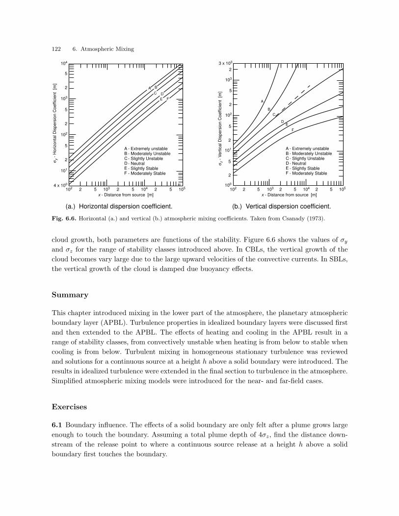
122 6. Atmospheric Mixing
(a.) Horizontal dispersion coefficient. (b.) Vertical dispersion coefficient.
A B C DE F
- Extremely unstable- Moderately Unstable- Slightly Unstable- Neutral- Slightly Stable- Moderately Stable
σy -
Horizonta
l D
ispers
ion C
oeffic
ient [m
]
x - Distance from source [m]
102 2 5 103 2 5 104 2 5 1054 x 100
101
2
5
102
2
5
103
2
5
104
A B
C D
E F
A B C DE F
- Extremely unstable- Moderately Unstable- Slightly Unstable- Neutral- Slightly Stable- Moderately Stable
x - Distance from source [m]
σz -
Vert
ical D
ispers
ion C
oeffic
ient [m
]
102 2 5 103 2 5 104 2 5 105100
2
5
101
2
5
102
2
5
103
2
3 x 10³
A
B
C
DE
F
Fig. 6.6. Horizontal (a.) and vertical (b.) atmospheric mixing coefficients. Taken from Csanady (1973).
cloud growth, both parameters are functions of the stability. Figure 6.6 shows the values of σy
and σz for the range of stability classes introduced above. In CBLs, the vertical growth of the
cloud becomes vary large due to the large upward velocities of the convective currents. In SBLs,
the vertical growth of the cloud is damped due buoyancy effects.
Summary
This chapter introduced mixing in the lower part of the atmosphere, the planetary atmospheric
boundary layer (APBL). Turbulence properties in idealized boundary layers were discussed first
and then extended to the APBL. The effects of heating and cooling in the APBL result in a
range of stability classes, from convectively unstable when heating is from below to stable when
cooling is from below. Turbulent mixing in homogeneous stationary turbulence was reviewed
and solutions for a continuous source at a height h above a solid boundary were introduced. The
results in idealized turbulence were extended in the final section to turbulence in the atmosphere.
Simplified atmospheric mixing models were introduced for the near- and far-field cases.
Exercises
6.1 Boundary influence. The effects of a solid boundary are only felt after a plume grows large
enough to touch the boundary. Assuming a total plume depth of 4σz, find the distance down-
stream of the release point to where a continuous source release at a height h above a solid
boundary first touches the boundary.
Exercises 123
6.2 Smoke-stack exhaust. A power company releases 1 kg/s of CO2 from a height of 30 m into
a wind with average velocity 4 m/s. The sky is partly cloudy and the terrain down-wind of the
release is pasture land. Estimate the turbulence intensities and find the maximum concentration
at ground level downstream of the release. How do the results change if the release point is
lowered by 15 m?
6.3 Urban roughness. The results presented in this chapter were for surfaces with uniform rough-
ness and elevations much greater than the roughness height z0. How do you expect relationships
for turbulence intensity to change near the street level in an urban setting (where the roughness
is largely due to buildings and houses)?

124 6. Atmospheric Mixing

7. Water Quality Modeling
Until now we have derived governing equations for and sought solutions to idealized cases where
analytical solutions could be found. Many problems in the natural world, however, are complex
enough that simplified analytical solutions are inadequate to predict the transport and mixing
behavior. In these situations, approximations of the governing transport equations (such as finite
difference) must be made so that numerical solutions can be found. These approximations can
be simple or complex, but often result in a large number of equations that must be solved
to predict the concentration distribution. Hence, computer algorithms are used to make the
numerical solutions tractable.
In this chapter, we introduce the field of water quality modeling based on computerized (nu-
merical or digital) tools. This chapter begins by outlining how to select an appropriate numerical
tool. The next two section describe common computer approximations. First, simple numerical
models based on plug-flow and continuously-stirred tank reactors are introduced. Second, an
overview of numerical approximations to the governing equations is presented. Because we are
now dealing with approximate solutions, new procedures are needed to assure that our results
are acceptable. The final section outlines the crucial steps necessary to test the accuracy of a
numerical result. Although computer power is rapidly growing, it remains important to use sim-
ple tools and thorough testing in order to understand and synthesize the meaning of numerical
results.
7.1 Systematic approach to modeling
A model is any analysis tool that reduces a physical system to a set of equations or a reduced-
scale physical model. Moreover, all of the solutions in previous chapters are analytical models of
natural systems. Whether analytical or numerical, the main question the modeler must answer
is: which model should I use?
7.1.1 Modeling methodology
The ASCE & WPCF (1992) design manual Design and Construction of Urban Stormwater
Management Systems outlines a four-step selection processes for choosing a water quality analysis
tool. These steps are discussed in detail in the following and include (1) defining project goals, (2)
describing an acceptable modeling tool, (3) listing the available tools that could satisfy the goals
and model description, and (4) selecting the model to be used based on an optimal compromise
between goals and available tools.
Copyright c© 2004 by Scott A. Socolofsky and Gerhard H. Jirka. All rights reserved.

126 7. Water Quality Modeling
1. Define project goals. It may sound like an obvious first step, but it is essential and,
regrettably, often overlooked: define the project goals before even choosing the model. Fischer
et al. (1979) emphasize this step as well, saying that the choice of a model depends crucially on
what the model is to do. Modeling goals are quite variable, ranging from the practical (provide
the analysis necessary to get the client his discharge permit) to the research oriented (develop a
new tool that overcomes some current modeling shortfall).
During this step, as much as possible should be learned about the system to be modeled.
Fischer et al. (1979) suggest that if possible, the investigator should become personally familiar
with the water body by going out on it in the smallest boat that is safe. Then, before venturing
near a computer or a model basin, he or she should make all possible computations, being
approximate where necessary, but seeking a feel for what the model will predict. Only after we
understand our system can we formulate appropriate project goals. In the words of the famous
landscape photographer Ansel Adams, “Visualization is of utmost importance; many failures
occur because of our uncertainty about the final image” (quoted in Fischer et al. (1979)). During
this stage one begins to formulate the necessary attributes of the model. This leads naturally
the next step.
2. Describe an acceptable modeling tool. Before selecting the model for the analysis,
formulate a list of abilities and characteristics that the model must have. These can include
things like input/output flexibility, common usage in the regulatory community, and physical
mixing processes the model must include. Our simplified predictions from step 1 of how the
system behaves are used in this step to formulate the model requirements. For instance, if we
expect rapid near-field mixing, we may suggest using a one-dimensional model. This step should
keep in mind what models are available, but not limit the analysis to known tools if they would
be inadequate to meet the project goals. In this stage the project goals may also need to be
revised. If the only acceptable modeling tool to meet a particular goal is too costly in terms
of computation time and project resources, perhaps that goal can be reformulated within a
reasonable project scope. The purpose, therefore, of this step is to optimize the modeling goals
by describing practical requirements of the modeling tool.
3. List applicable tools. Once the analysis tool has been adequately described, one must
formulate a list of available tools that meet these requirements. In engineering practice, we must
often choose an existing model with a broad user base. Appendix D lists several public-domain
models. Most of them are available free of charge from government sponsor agencies, but some
are also commercial. The purpose of choosing an existing model is that it has been thoroughly
tested by many previous users and that the regulatory agencies are accustomed to seeing and
interpreting its output. However, available tools may not always be adequate to meet the project
goals.
If existing tools are inadequate, then a new tools must be developed, and a list of existing
methods is an important step. Methods are the building blocks of models. A one-dimensional
finite difference model employs two methods: a one-dimensional approximation and a finite
difference numerical scheme. Going a step deeper, the finite-difference method can have many
attributes, such as forward, central, or backward differencing, implicit or explicit formulation,

7.1 Systematic approach to modeling 127
and first-, second-, or higher-order solution algorithms. Section 7.3 describes what some of these
terms mean. The point is that, when designing a new tool, there are many existing building
blocks from which to choose, and these can be quite helpful. It may turn out that simply adding
an unsteady algorithm to an existing steady-state model will meet the project goals. Hence,
knowing as much as possible about existing models and methods is essential to implementing
and/or designing an analysis tool.
4. Make an optimal compromise between goals and available tools. In the final step
of choosing a modeling tool, we seek an optimal compromise between the project goals and
the available tools. This is where the decision to proceed with a given modeling tool is made.
The project goals are the guide to choosing the model. It sounds simple, but choose the best
model to meet the project goals, not just the best available model. As computers become faster,
the tendency is to just pick the biggest, boldest model and to force it to meet your needs.
However, the enormous amount of output from such a model may be overwhelming and costly
and unnecessary in the light of certain project goals. Therefore, choose the most appropriate,
simplest model that also satisfies the scientific rigor of the project goals, and when necessary,
develop new tools.
7.1.2 Issues of scale and complexity
Throughout the process of choosing a modeling tool one is confronted with issues of system
scale and complexity. The world is inherently three-dimensional and turbulent, but with current
computer resources, we must often limit our analysis to one- and two-dimensional approximations
with turbulence closure schemes that approximate the real world. Hence, we must make trade
offs between prototype complexity and model ability.
We can evaluate these trade offs by doing a scale analysis to determine the important scales
in our problem. This is the essence of steps one and two, above, where we try to predict what
the model will tell us and use this information to characterize the needed tool. For transport
problems, we must consider the advective, diffusing reaction equation. For illustration, consider
a first-order reaction
∂C
∂t+
∂(uC)
∂x+
∂(vC)
∂y+
∂(wC)
∂z= Dx
∂2C
∂x2+ Dy
∂2C
∂y2+ Dz
∂2C
∂z2± kC. (7.1)
This equation has three unit scales: mass, time, and length. It also has three processes: advection,
diffusion, and reaction. We would like to formulate typical scales of these three processes from
the typical units in the problem. For example, the advection time scale is the time it takes
for fluid to move through our system. If we are modeling a river reach of length L with mean
velocity U , then the advective time scale is
Ta = L/U. (7.2)
Processes that occur on time scales much shorter than Ta can neglect advection. We can use these
scales to non-dimensionalize the governing equation. To do this, we define the non-dimensional
variables using primes as follows
128 7. Water Quality Modeling
x = Lxx′; y = Lyy′
z = Lzz′; u = Uu′
v = V v′; w = Ww′
C = C0C′; t = T0t
′
k = 1/Trk′ (7.3)
where the upper-case variables are typical scales in the problem. For example T0 is an external
time scale, such as a discharge protocol or the diurnal cycle and Tr is the reaction time scale,
such as the half-life for a dye-off reaction. The L’s are system dimensions and U , V , and W are
average velocities. Substituting into (7.1) gives
1
T0
∂C ′
∂t′+
U
Lx
∂(u′C ′)
∂x′ +V
Ly
∂(v′C ′)
∂y′+
W
Lz
∂(w′C ′)
∂z′=
Dx
L2x
∂2C ′
∂x′2 +Dy
L2y
∂2C ′
∂y′2+
Dz
L2z
∂2C ′
∂z′2± 1
T1/2k′C ′. (7.4)
Note that to make this equation fully non-dimensional, we must multiple each term by a time
scale, for example T0. We can now determine the relative importance of each term by considering
their leading coefficients. Comparing the convective terms
Longitudinal advection
Lateral advection=
U
V· Ly
Lx(7.5)
Longitudinal advection
Vertical advection=
U
W· Lz
Lx(7.6)
If these ratios are much greater than one, then longitudinal advection is the only advection term
that we must keep in the equation. Thus, the importance of a given convection term depends
on the velocity scales in our problem and the length of river we are considering. In many river
problems, these ratios are much greater than one, and we only keep the longitudinal advection
term. Likewise, we can compare the diffusion terms to the advection term. For longitudinal
diffusion we have
Longitudinal diffusion
Longitudinal advection=
Dx
L2xTa
(7.7)
which is our familiar Peclet number. For large Peclet numbers, we only consider diffusion, and for
small Peclet numbers, we only consider advection. Hence, the important terms in the equation
again depend on the length of river we are considering.
As an example, when might a one-dimensional steady-state model with dye-off be an accept-
able model for a given river reach? The governing model equation would be
u∂C
∂x= Dx
∂2C
∂x2− kC. (7.8)
By comparing with the non-dimensional equation above, this equation implies several constraints
on the river. Consider first the external time-scale. This model implies
UT0
Lx 1. (7.9)

7.2 Simple water quality models 129
For the convective terms, this model implies that
ULy
V Lx 1 (7.10)
ULz
WLx 1 (7.11)
or alternatively
∂C
∂y=
∂C
∂z= 0. (7.12)
Similarly, for diffusion this model implies that
UL2y
LxDy 1 (7.13)
UL2z
LxDz 1 (7.14)
or, again, alternatively
∂C
∂y=
∂C
∂z= 0. (7.15)
Finally, for the reaction, this model implies that
UT1/2
Lx≈ 1. (7.16)
Therefore, by comparing the relevant scales in our problem to the approximations made by
models, we can determine just how complex the model must be to approximate our system
adequately.
7.1.3 Data availability
As a final comment on the selection and implementation of an analysis tool, we discuss a few
points regarding the data that are used to validate the model (Section 7.4 below discusses how to
test a model in more detail). The only test available to determine whether the model adequately
reproduces our natural system is to compare model output to data (measurements) taken from
the prototype system. In general, as the model complexity increases, the number of parameters
we can use to adjust the model results to match the prototype also increases, giving us more
degrees of freedom. The more degrees of freedom we have, the more data we need to calibrate
our model. Hence, the data requirements of a model are directly proportional to the model
complexity. If very limited data are available, then complex models should be avoided because
they cannot be adequately calibrated or validated.
7.2 Simple water quality models
Some simple water quality models can be developed for special cases where advection or diffusion
is dominant. As introduced in Chapter 2, the Peclet number is a measure of diffusion to advection
dominance. The Peclet number, Pe, is defined as

130 7. Water Quality Modeling
Q Q
Fig. 7.1. Schematic of a plug-flow reactor.
Pe =D
uL(7.17)
=D
u2t(7.18)
where the two definitions are equivalent. The Peclet number is small when advection is dominant
and large when diffusion is dominant. Two simple models can be developed for the limiting cases
of Pe → 0 and Pe → ∞. A third hybrid model is also introduced in this section for simplified
application to arbitrary Pe.
7.2.1 Advection dominance: Plug-flow reactors
For Pe → 0 we can neglect longitudinal diffusion and dispersion, and we have the so-called
plug-flow reactor. Shown in Figure 7.1, a slab of marked fluid is advected with the mean flow,
perhaps undergoing reactions, but not spreading in the lateral. Taking D = 0, the governing
reactive transport equation becomes
∂C
∂t+ u
∂C
∂x= ±R. (7.19)
To solve this equation, we make the familiar coordinate transformation to move our coordinate
system with the mean flow. That is,
ξ = x − ut (7.20)
τ = t. (7.21)
As demonstrated in Chapter 2, using the chain rule to substitute this coordinate transformation
into (7.19) gives
∂C
∂τ= ±R (7.22)
which is easily solved after defining an initial condition and the transformation reaction R.
For example, consider a first-order die-off reaction for a slab with initial concentration C0.
The solution to (7.22) is
C(τ) = C0 exp(−kτ) (7.23)
or in the original coordinate system, we have the interchangeable solutions
C(t) = C0 exp(−kt) (7.24)
C(x) = C0 exp(−kx/u). (7.25)
The residence time for a plug-flow reactor depends on the distance of interest L0. From the
definition of residence time
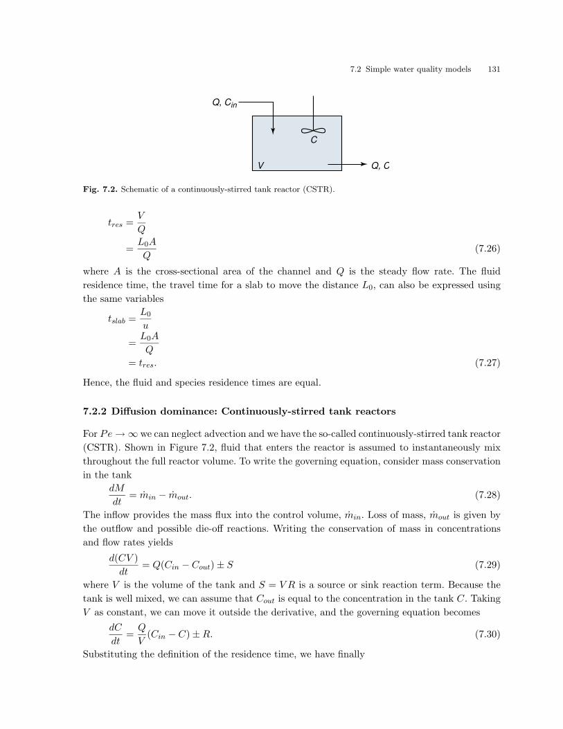
7.2 Simple water quality models 131
V
C
Q, C
Q, Cin
Fig. 7.2. Schematic of a continuously-stirred tank reactor (CSTR).
tres =V
Q
=L0A
Q(7.26)
where A is the cross-sectional area of the channel and Q is the steady flow rate. The fluid
residence time, the travel time for a slab to move the distance L0, can also be expressed using
the same variables
tslab =L0
u
=L0A
Q
= tres. (7.27)
Hence, the fluid and species residence times are equal.
7.2.2 Diffusion dominance: Continuously-stirred tank reactors
For Pe → ∞ we can neglect advection and we have the so-called continuously-stirred tank reactor
(CSTR). Shown in Figure 7.2, fluid that enters the reactor is assumed to instantaneously mix
throughout the full reactor volume. To write the governing equation, consider mass conservation
in the tank
dM
dt= min − mout. (7.28)
The inflow provides the mass flux into the control volume, min. Loss of mass, mout is given by
the outflow and possible die-off reactions. Writing the conservation of mass in concentrations
and flow rates yields
d(CV )
dt= Q(Cin − Cout) ± S (7.29)
where V is the volume of the tank and S = V R is a source or sink reaction term. Because the
tank is well mixed, we can assume that Cout is equal to the concentration in the tank C. Taking
V as constant, we can move it outside the derivative, and the governing equation becomes
dC
dt=
Q
V(Cin − C) ± R. (7.30)
Substituting the definition of the residence time, we have finally

132 7. Water Quality Modeling
dC
dt=
1
tres(Cin − C) ± R (7.31)
which is the governing equation for a CSTR.
Consider first the conserving case, where R = 0. Taking the initial condition as a clean tank
C0 = 0, the solution to (7.31) is
C(t) = Cin
[
1 − exp
(
− t
tres
)]
. (7.32)
Thus, the concentration in the tank increases exponentially with a rate constant k = 1/tres. The
concentration in the tank reaches steady state asymptotically. If we define steady state as the
time, tss, until C = 0.99C0, then
tss = 4.6tres. (7.33)
Therefore, without reactions, steady state is reached in about 4.6 residence times.
The solution for the reacting case is slightly more complicated because (7.31) is an inhomo-
geneous differential equation with forcing function ±R. Consider the case of a first-order die-off
reaction and an initial tank concentration of C0 = 0. Assuming a particular solution (refer to
Appendix C for an example of solving an inhomogeneous equation) of the form Cp = ACin, the
solution is found to be
C(t) =Cin
1 + ktres
[
1 − exp
[
−(
1 + ktres
tres
)
t
]]
. (7.34)
Because of the reaction, the steady state concentration in the tank is no longer the inflow
concentration, but rather
Css =Cin
1 + ktres(7.35)
and the coefficient 1/(1 + ktres) is one minus the removal rate. The time to reach steady state,
tss, is the time to reach 0.99Css or
tss =4.6tres
1 + ktres. (7.36)
7.2.3 Tanks-in-series models
The simplest type of river-flow model that incorporates some form of diffusion or dispersion
is the tanks-in-series model, which is a chain of linked CSTRs. An example tanks-in-series
model is shown in Figure 7.3. In the example each tank has the same dimensions, and the flow
rate is constant. The method also works for variable volume tanks, and under gradually-varied
flow conditions, stage-discharge relationships can be used to route variable flows through the
tanks. To see why the tanks-in-series model produces diffusion, consider an instantaneous pulse
injection in the first tank. The outflow from that tank would be the solution to the CSTR given
by (7.32). The outflow from the first tank is, therefore, exponential, clearly not the expected
Gaussian distribution. But, this outflow goes into the next tank. At first, that tank is clean,
and the little bit of tracer entering the tank in the beginning is quickly diluted; hence, the
outflow concentration starts at zero and increases slowly. Eventually, a large amount of the
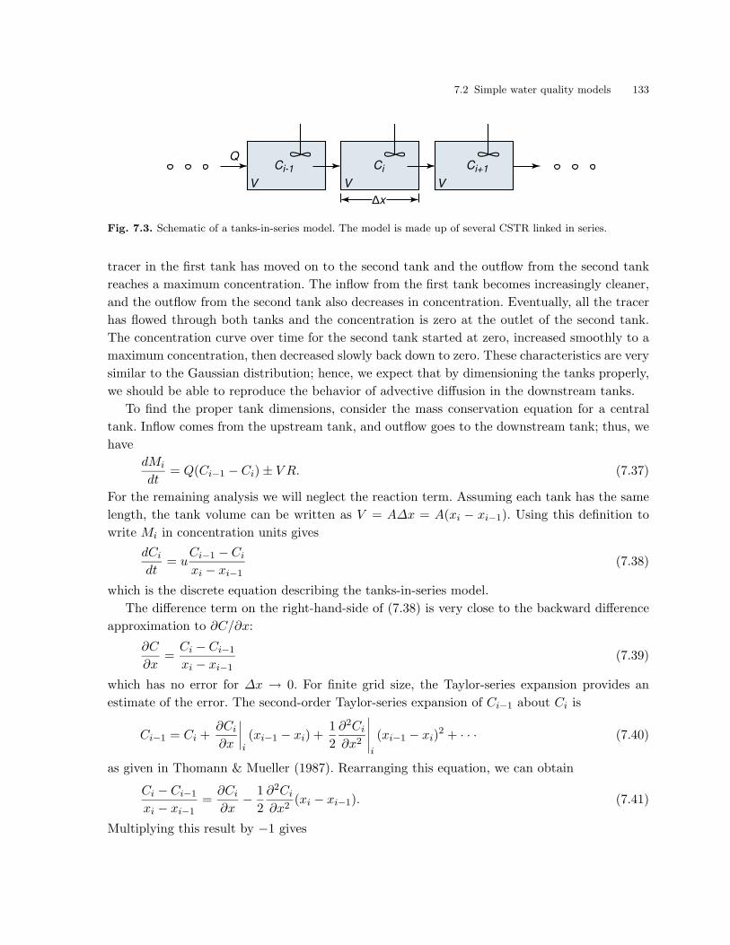
7.2 Simple water quality models 133
V V V
CiCi-1 Ci+1
Q
∆x
Fig. 7.3. Schematic of a tanks-in-series model. The model is made up of several CSTR linked in series.
tracer in the first tank has moved on to the second tank and the outflow from the second tank
reaches a maximum concentration. The inflow from the first tank becomes increasingly cleaner,
and the outflow from the second tank also decreases in concentration. Eventually, all the tracer
has flowed through both tanks and the concentration is zero at the outlet of the second tank.
The concentration curve over time for the second tank started at zero, increased smoothly to a
maximum concentration, then decreased slowly back down to zero. These characteristics are very
similar to the Gaussian distribution; hence, we expect that by dimensioning the tanks properly,
we should be able to reproduce the behavior of advective diffusion in the downstream tanks.
To find the proper tank dimensions, consider the mass conservation equation for a central
tank. Inflow comes from the upstream tank, and outflow goes to the downstream tank; thus, we
have
dMi
dt= Q(Ci−1 − Ci) ± V R. (7.37)
For the remaining analysis we will neglect the reaction term. Assuming each tank has the same
length, the tank volume can be written as V = A∆x = A(xi − xi−1). Using this definition to
write Mi in concentration units gives
dCi
dt= u
Ci−1 − Ci
xi − xi−1(7.38)
which is the discrete equation describing the tanks-in-series model.
The difference term on the right-hand-side of (7.38) is very close to the backward difference
approximation to ∂C/∂x:
∂C
∂x=
Ci − Ci−1
xi − xi−1(7.39)
which has no error for ∆x → 0. For finite grid size, the Taylor-series expansion provides an
estimate of the error. The second-order Taylor-series expansion of Ci−1 about Ci is
Ci−1 = Ci +∂Ci
∂x
∣
∣
∣
∣
i(xi−1 − xi) +
1
2
∂2Ci
∂x2
∣
∣
∣
∣
∣
i
(xi−1 − xi)2 + · · · (7.40)
as given in Thomann & Mueller (1987). Rearranging this equation, we can obtain
Ci − Ci−1
xi − xi−1=
∂Ci
∂x− 1
2
∂2Ci
∂x2(xi − xi−1). (7.41)
Multiplying this result by −1 gives

134 7. Water Quality Modeling
Ci−1 − Ci
xi − xi−1= −∂Ci
∂x+
1
2
∂2Ci
∂x2(xi − xi−1) (7.42)
which can be substituted immediately for the right-hand-side of (7.38) leaving
dCi
dt= −u
∂Ci
∂x+
u(xi − xi−1)
2
∂2Ci
∂x2. (7.43)
Dropping the subscripts and recognizing ∆x = (xi − xi−1) gives the governing equation
dC
dt+ u
∂C
∂x=
u∆x
2
∂2C
∂x2. (7.44)
Thus, our derived governing equation for a tanks-in-series model has the same form as the
advective diffusion equation with a diffusion coefficient of Dn = u∆x/2.
The effective diffusion coefficient, Dn, for a tanks-in-series model is actually a numerical
error due to the discretization. As the discretization becomes more course, the numerical error
increases and the numerical diffusion goes up. For ∆x → 0, the numerical diffusion vanishes,
and we have the plug-flow reactor. Hence, for a tanks-in-series model, we choose the tank size
such that Dn is equal to the physical longitudinal diffusion and dispersion in the river reach.
7.3 Numerical models
Although the tank-in-series model was shown to be a special discretization of the advective
diffusion equation, other numerical techniques specifically set out to discretize the governing
equation. For our purposes, a numerical model is any model that seeks to solve a differential
equation by discretizing that equation on a numerical grid.
7.3.1 Coupling hydraulics and transport
To simulate chemical transport, the velocity field, represented by u in the transport equation
must also be computed. The model that calculates u is called the hydrodynamic or hydraulic
model. Thus, to simulate transport, the hydrodynamic and transport models must be properly
coupled.
Whether the hydrodynamic and transport models must be implicitly coupled or whether
they can be run in series depends on the importance of buoyancy effects. If the system is free
from buoyancy effects, the hydrodynamics are independent of the transport; hence, they can
be run first and their output stored. Then, many transport simulations can be run using the
hydrodynamic data without re-running the hydrodynamic code. If buoyancy effects are present
in the water body, then the transport of buoyancy (heat or salinity or both) must be coupled with
the hydrodynamics, and both models must be run together. Once the output from the coupled
model is stored, further transport simulations can be run for constituents that do not influence
the buoyancy (these are called passive constituents). Because the hydrodynamic portion of the
model is computationally expensive, the goal in transport modeling is to de-couple the two
models as much as possible.
7.3 Numerical models 135
7.3.2 Numerical methods
There are probably as many numerical methods available to solve the coupled hydrodynamic
and advective transport equations as there are models; however, most models can be classified
by a few key words.
There are three main groups of numerical methods: finite difference, finite volume, and finite
element. For special selections of basis functions and geometries, the three methods can all be
made equivalent, but in their standard applications, the methods are all slightly different. The
finite difference method is built up from a series of nodes, the finite volume method is built up
from a group of cells, and the finite element method is made up of a group of elements, where
each element is comprised of two or more grid points. In the finite difference case, the differential
equation is discretized over the numerical grid, and derivatives become difference equations that
are functions of the surrounding cells. In the finite volume case, the fluxes through the cell
network are tracked and the differential equations are integrated over the cell volume. For finite
elements, a basis function is chosen to describe the variation of an unknown over the element and
the coefficients of the basis functions are found by substituting the basis functions as solutions
into the governing equations. Because finite difference methods are easier to implement and
understand, these methods are more widely used.
A numerical method may further be explicit or implicit. An explicit scheme is the easiest
to solve because the unknowns are written as functions of known quantities. For instance, the
concentration at the new time is dependent on concentrations at the previous time step and
at upstream (known) locations. In an implicit scheme, the equations for the unknowns are
functions of other unknown quantities. For instance, the concentration at the new time may
depend on other concentrations at the new time or on downstream locations not yet computed.
In the implicit case, the equations represent a system of simultaneous equations that must be
solved using matrix algebra. The advantage of an implicit scheme is that it generally has greater
accuracy.
Finally, numerical methods can be broadly categorized as Eulerian or Lagrangian. Eulerian
schemes compute the unknown quantities on a fixed grid based on functions of other grid quan-
tities. Lagrangian methods use the method of characteristics to track unknown quantities along
lines of known value. For instance, in a Lagrangian transport model, the new concentration at
a point could be found by tracking the hydrodynamic solution backward in time to find the
point where the water parcel originated and then simply advecting that concentration forward
to the new time. Because the Lagrangian method relies heavily on the velocity field, small er-
rors in the velocity field (particularly for fields with divergence) can lead to large errors in the
conservation of mass. The advantage of the Lagrangian method is that it can backtrack over
several hydrodynamic time steps; hence, there is no theoretical limitation on the size of the time
step in a Lagrangian transport model. An example of a one-dimensional Lagrangian scheme is
the Holly-Preissman method. By contrast, for the Eulerian model, the time step is limited by a
so-called Courant number restriction, that says that the time step cannot be so large that fluid
in one cell advects beyond the next adjacent cell over one time step. Mathematically, this can
be written as
136 7. Water Quality Modeling
∆t ≤ ∆x
u(7.45)
where ∆t is the time step and ∆x is the grid size.
7.3.3 Role of matrices
In the case of explicit models, matrices are not a necessity, but for implicit models and models
simulating many contaminant, matrices provide a comfortable (and often necessary) means of
solving the governing equations. For an implicit scheme, the equations for a given node at the
new time are dependent on the solutions at other nodes at the same time. This means that
implicit schemes are inherently a system of equations (sometimes non-linear), which are best
solves with matrices. The general matrix equation is
Ax = b (7.46)
where A is an n x n matrix of equation coefficients, x is an n x 1 vector of unknowns (for
example, flow rates), and b is an n x 1 vector of forcing functions. Writing the equations in such
a way makes derivation of the model equations manageable and implementation in the computer
algorithm straightforward. The solution of (7.46) is
x = A−1b (7.47)
where A−1 is the matrix inverse. Most computer languages have built-in methods for solving
matrices. For the non-linear case, an iteration technique must be employed. A common method
is the Newton-Raphson method.
7.3.4 Stability problems
One limitation already mentioned for an Eulerian transport scheme is the Courant number
restriction. In general, all schemes have a range of similar restrictions that limit the allowable
spatial grid size and time step such that the scheme remains stable. If the time step is set
longer than such a constraint, the model is unstable and will give results with large errors that
eventually blow up. The full hydrodynamic equations are hyperbolic and generally have more
stringent limitations than the parabolic transport equation. Before implementing a model, it is
advised to seek out the published stability criteria for the model; this can save a lot of time in
getting the model to run smoothly.
7.4 Model testing
An unfortunate fact of numerical modeling is that implementation and calibration is very time
consuming, and little time is available for a thorough suite of model tests. This does not excuse
the fact that model testing is necessary, but rather explains why it is often neglected. Even
when using well-known tools, the following suite of tests is imperative to ensure that the model
is working properly for your application. The following tests are specific to transport models,
but apply in a generalized sense to all models.

7.4 Model testing 137
7.4.1 Conservation of mass
All transport (water quality models) must conserve mass! This is a zeroth-order test that con-
firms whether the zeroth-moment of the concentration distribution is accurately reproduced in
the solution. Clearly, when reactions are present, a given species may be loosing or gaining mass
due to the reaction. This test must confirm, then, that the total system mass remains constant
and that a species only gains mass at the rate allowed by the reaction equation. This test is
often conducted in conjunction with the next test. However, it should always also be conducted
for the complex real-world case being simulated, where analytical solutions are not available.
7.4.2 Comparison with analytical solutions
The model should be tested in idealized conditions to compare its results to known analytical
solutions. This test confirms whether the model actually solves the governing equation that it
was designed to solve. Deviations may be caused by many sources, most notably programming
errors and numerical inaccuracy. Although most widely used models are free from programming
errors, this cannot be tacitly assumed. In this author’s experience, programming errors have been
found in well-known, government-supported models by running this test. The issue of numerical
inaccuracy arises due to the discretization, as in the case of numerical diffusion mentioned for
the tanks-in-series model described above. Hence, the idealized case should have length and
time scales as close to the prototype as possible in order to accurately assess the importance of
numerical inaccuracy arising from the numerical method and the discretization.
This step can save a lot of time in applying the model to the prototype because the source
of errors can often be identified faster in idealized systems. First, the analytical solution is a
known result. If the model gives another result, the model must be wrong. Second, the complexity
of the real-world case makes it difficult to assess the importance of deviations from measured
results. Once the model has been thoroughly tested against analytical results, deviations can
be explained by physical phenomena in the prototype not present or falsely implemented in the
model. Third, this test helps determine the stability requirements for complex models.
7.4.3 Comparison with field data
Only after it is certain that the model is solving the equations properly and within a known
level of error can the model be compared to field or laboratory measurements of the prototype.
The comparison of model results with these date serves two purposes. First, the model must
be calibrated; that is, its parameters must be adjusted to match the behavior of the prototype.
Second the model must be validated. This means that a calibrated model must be compared to
data not used in the calibration to determine whether the model is applicable to cases outside
the calibration data set. These prototype measurements fall into two categories: tracer studies
and data collection of natural events.

138 7. Water Quality Modeling
Tracer studies. In a tracer study, dye is injected into the natural system, and concentrations
are measured in time and space to record how the dye is transported and diluted. The advantage
of a tracer study is that the source injection rate and location are known with certainty and that
reactions can (often) be neglected. Tracer studies help calibrate the model parameters (such as
diffusion and dispersion coefficients and turbulent closure schemes) to the real-world case. These
studies also help to confirm whether the model assumptions are met (such as the one-dimensional
approximation) and are good tests of both the hydrodynamic and water quality models.
Water quality data. The final set of data available for model testing is actual measurements
of the modeled constituents in the prototype under natural conditions. These measurements
represent true values, but are difficult to interpret because of our incomplete description of the
prototype itself. We often do not know the total loading of constituent, and all the model equa-
tions are approximations of the actual physical processes in the prototype. These measurements
further help to confirm whether the model assumptions are valid and to calibrate model parame-
ters. Once the tests listed above are completed, the modeler should have a good understanding of
how the complex physical processes in the model combine to give the model results. Deviations
between the model and the field measurements should then be explained through the physical
insight available in the model.
It is important to point out that the water quality measurement campaign should compliment
the output available from the model. That is, the data should be collected such that they can
be used to calibrate and test the model. If the model only outputs daily predictions, then the
measurements should be able to predict daily values; instantaneous point measurements are only
useful for a parameter that does not vary much over the diurnal cycle. In summary, the model
is only as good as the data that support it, and the data must be compatible with the model
and flex the parts of the model that are the most uncertain.
Summary
This chapter introduced the concept of water quality modeling. A model is defined as any analy-
sis tool that reduces a physical system to a set of equations or a reduced-scale physical model. A
four-step procedure was suggested to help select the appropriate model: (1) define project goals,
(2) describe an acceptable modeling tool, (3) list the available tools that could satisfy the goals
and model description, and (4) select the model to be used based on an optimal compromise
between goals and available tools. Because analytical solutions are not always adequate, nu-
merical techniques were introduced. These included tank reactor models and numerical solution
methods for differential equations, such as finite difference and finite element. Because numerical
solutions result in a large number of calculations, a rigorous procedure for testing a numerical
model was also suggested. These steps include (1) confirming that model conserves mass, (2)
testing the model in idealized cases against analytical solutions, and (3) comparing the model
to field data in the form of dye studies and the collection of water quality data. Good modeling
projects should follow all of these suggested procedures.

Exercises 139
0 5 10 15 20 25 30 350
0.5
1
1.5
2
2.5
3
3.5Measured dye concentration breakthrough curve
Time since injection start [min]
Con
cent
ratio
n [m
g/l]
Fig. 7.4. Measured dye concentration for example dye study. Dye fluctuations are due to instrument uncertainty,not due to turbulent fluctuations.
Exercises
7.1 Equation scaling. Non-dimensionalize the one-dimensional momentum equation
∂u
∂t+ u
∂u
∂x=
1
ρ
∂p
∂x+ ν
∂2u
∂x2(7.48)
using the non-dimensional variable definitions
u = U0u′ ; x = Lx′ (7.49)
t = (L/U0)t′ ; p = ρU2
0 p′ (7.50)
Divide the equation by the coefficient in front of ∂u′/∂t′. What familiar non-dimensional number
becomes the leading coefficient of the viscous term? When is the viscous term negligible?
7.2 Finite difference. Write the explicit backward-difference approximation to the reaction equa-
tion
dC
dt= kC. (7.51)
Program this solution in a computer and suggest a criteria for selecting the appropriate time
step ∆t by comparing to the analytical solution
C(t) = C0 exp(kt). (7.52)
7.3 Tanks-in-series model. A river has a cross-section of h = 1 m deep and B = 10 m wide.
The mean stream velocity is 22.5 cm/s. A dye study was conducted my injecting 2.25 g/s of dye
uniformly across the cross-section 150 m upstream of a measurement point. The measurements
of dye concentration at L = 150 m are given in Figure 7.4. From the figure, determine the value
of the dispersion coefficient. Based on this value, how many tanks in a tanks-in-series model
would be needed to reproduce this level of dispersion in the numerical model?

140 7. Water Quality Modeling
A. Point-source Diffusion in an Infinite Domain:
Boundary and Initial Conditions
In this appendix we discuss how the boundary and initial conditions for a point source in an
infinite, one-dimensional domain are applied to find the solution of the diffusion equation. The
governing equation is
∂C
∂t= D
∂2C
∂x2(A.1)
with boundary conditions C(±∞, t) = 0 and initial condition C(x, 0) = (M/A)δ(x) (for more
detail, refer to Chapter 1).
In this case we will use the Fourier exponential transform instead of the similary method to
obtain our result. Although each method is equally valid, it is easier to see how the boundary
conditions are applied using the Fourier transform. Since the governing equations that is obtained
after applying the boundary conditions will be the same using either method, applying the
Fourier transform method here is the better approach. For this method we use the Fourier
exponential transformation defined by
F(α, t) =
∫ ∞
−∞F (x, t)e−iαxdx (A.2)
where F(α, t) is the Fourier transformation of F (x, t), α is a transformation variable, and i is
the imaginary number. This method implicitly satisfies the boundary conditions at ±∞. This is
called a behavioral boundary condition (see e.g. Boyd 1989), and it is not necessary to apply the
boundary to fix the values of integration constants—the solution implicitely obeys the boundary
conditions because of our use of the Fourier transform. The following application of this method
to the diffusion equation is taken from Mei (1997).
The Fourier transform of the governing diffusion equation gives
dCdt
+ Dα2C = 0. (A.3)
The power of the Fourier transform is that it converts partial differential equations into ordinary
differential equations, this time a simple, first-order ODE with solution
C(α, t) = F(α) exp(−Dα2t). (A.4)
F(α) is found by applying the initial condition. Applying the Fourier transform to the initial
condition gives
F(α) = C(α, 0)
=
∫ ∞
−∞(M/A)δ(x)e−iαxdx
Copyright c© 2004 by Scott A. Socolofsky and Gerhard H. Jirka. All rights reserved.
142 A. Point-source Diffusion in an Infinite Domain: Boundary and Initial Conditions
= M/A. (A.5)
The drawback of the Fourier transform method is that the inverse transform to get back to our
desired dimensional space is sometimes a difficult integral.
We stop here to take a look at what we have done so far. The Fourier transform method
implicitly satisfies the boundary conditions; therefore, we do not have to think about them
anymore. Further, the initial condition was used to find the solution to the ODE obtained after
the Fourier transform. Thus, our solution
C(α, t) = (M/A) exp(−Dα2t) (A.6)
satisfies all our boundary and initial conditions. The remaining task is to perform a Fourier
inverse transform on this solution.
The Fourier inverse transform is defined in general as
F (x, t) =1
2π
∫ ∞
−∞F(α, t)eiαxdα. (A.7)
For our problem, the inverse transform becomes
C(x, t) =1
2π
∫ ∞
−∞(M/A) exp(−Dα2t)eiαxdα. (A.8)
We can simplify a little by recognizing that eiαx = cos(αx) + i sin(αx). Since e−Dα2t is an even
function and i sin(αx) is an odd function, we can neglect the sin-contribution, leaving us with
the integral
C(x, t) =M
2πA
(
2
∫ ∞
0e−Dα2t cos(αx)dα
)
(A.9)
which we still must solve.
The first step in solving (A.9) is to simplify the exponential using the change of variable
α =x√Dt
(A.10)
dα =dx√Dt
(A.11)
(note, this in an arbitrary change of variable that puts the integral in a form more likely to be
found in integral tables). Further, we define a new variable
η =x√Dt
(A.12)
(note, this is also an arbitrary decision). Substituting these definitions leaves us with
C(x, t) =M
πA√
Dt
∫ ∞
0e−x2
cos(ηx)dx. (A.13)
Thus, our solution simplifies to having to solve the integral
I(η) =
∫ ∞
0e−x2
cos(ηx)dx. (A.14)
The integral in (A.14) is not a trivial integral, but can be solved by employing the following
tricks. Basically, we need to find the derivative of I with respect to η and then put it in a useful
form. We begin with
A. Point-source Diffusion in an Infinite Domain: Boundary and Initial Conditions 143
dI
dη=
∫ ∞
0−xe−x2
sin(ηx)dx. (A.15)
Next, recognize that xdx = (1/2)d(x2), giving
dI
dη= −1
2
∫ ∞
0e−x2
sin(ηx)d(x2). (A.16)
Similarly, we make use of the identity e−x2
d(x2) = −d(e−x2
), which lets us write
dI
dη=
1
2
∫ ∞
0sin(ηx)d(e−x2
). (A.17)
Now, we integrate by parts (where u = sin(ηx) and dv = d(e−x2
)) yielding
dI
dη=
1
2(e−x2
sin(ηx))
∣
∣
∣
∣
∞
0− 1
2
∫ ∞
0e−x2
d(sin(ηx))
= 0 − η
2
∫ ∞
0e−x2
cos(ηx)dx
= −η
2I(η). (A.18)
We can rearrange the last line as follows
dI
dη+
η
2I(η) = 0 (A.19)
which looks remarkably like (1.49) if C0 is taken as zero. The initial condition necessary to solve
the above ODE is given by
I(0) =
∫ ∞
0e−x2
dx. (A.20)
If we convert I in the previous two equations to our variables used in the similarity solution,
we obtain
df
dη+
η
2f(η) = 0 (A.21)
with initial condition∫ ∞
−∞f(η)dη = 1. (A.22)
Therefore, we have shown through a rigorous application of the Fourier transform method, that
the above two equations give the solution to the diffusion equation that we seek in an infinite
domain for an instantaneous point source after having applied the appropriate boundary and
initial conditions.
144 A. Point-source Diffusion in an Infinite Domain: Boundary and Initial Conditions

B. Solutions to the Advective Reacting
Diffusion Equation
This appendix presents solutions to the advective reacting diffusion equation given by
∂C
∂t+ u
∂C
∂x+ v
∂C
∂y+ w
∂C
∂z= Ex
∂2C
∂x2+ Ey
∂2C
∂y2+ Ez
∂2C
∂z2− kC (B.1)
for homogeneous, anisotropic turbulence with the steady velocity u = (u, v, w). The Ei’s are
the anisotropic turbulent diffusion coefficients, and k is a constant first-order decay rate. In
previous chapters we denoted the turbulent diffusion coefficient by Dt. We use Dt = E here so
that the subscripts do not get too complicate and to expose the reader to another notation for
the turbulent diffusion coefficient common in the literature.
B.1 Instantaneous point source
An instantaneous point source has an injection of mass, M , at the point x = (x1, y1, z1) at time
t = 0. The following solutions cover different ambient conditions.
B.1.1 Steady, uni-directional velocity field
For a steady velocity field u = (U, 0, 0), the solutions is
C(x, y, z, t) =M
4πt√
4πExEyEztexp
(
−((x − x1) − Ut)2
4Ext
− (y − y1)2
4Eyt− (z − z1)
2
4Ezt− kt
)
. (B.2)
B.1.2 Fluid at rest with isotropic diffusion
For isotropic diffusion, Ex = Ey = Ez = E, and, in a stagnant ambient without decay, (B.2)
simplifies to
C(x, y, z, t) =M
(4πEt)3/2exp
(
− r2
4Et
)
(B.3)
where r =√
x2 + y2 + z2 and x1 = y1 = z1 = 0.
Copyright c© 2004 by Scott A. Socolofsky and Gerhard H. Jirka. All rights reserved.

146 B. Solutions to the Advective Reacting Diffusion Equation
B.1.3 No-flux boundary at z = 0
The no-flux boundary condition at z = 0 is enforced by an image source at x = (x1, y1,−z1),
giving the solution for z > 0 neglecting decay and crossflow as
C(x, y, z, t) =M
4πt√
4πExEyEzt·
exp
(
−(x − x1)2
4Ext− (y − y1)
2
4Eyt− (z − z1)
2
4Ezt
)
+M
4πt√
4πExEyEzt·
exp
(
−(x − x1)2
4Ext− (y − y1)
2
4Eyt− (z + z1)
2
4Ezt
)
. (B.4)
B.1.4 Steady shear flow
The following solution, presented in Okubo & Karweit (1969), is for the special shear flow given
by u = (u0(t) + λyy + λzz, 0, 0), where λy and λz are the velocity gradients defined by
λy =∂u
∂y(B.5)
λz =∂u
∂z. (B.6)
The solution is
C(x, y, z, t) =M
4πt√
4πExEyEzt√
1 + φ2t2·
exp
−
(
x −∫ t0 u0(t
′)dt′ − 12(λyy + λzz)t
)2
4Ext(1 + φ2t2)
− y2
4Eyt− z2
4Ezt− kt
)
, (B.7)
where the injection is at (0, 0, 0) and φ2 is given by
φ2 =1
12
(
λ2y
Ey
Ex+ λ2
z
Ez
Ex
)
. (B.8)
B.2 Instantaneous line source
An instantaneous line source has an injection of mass, m′, per unit length along the line through
x = (x1, y1) for z = ±∞ at time t = 0. The following solutions cover different ambient conditions.
B.2.1 Steady, uni-directional velocity field
For a steady velocity field u = (U, 0, 0), the solutions is
B.4 Continuous point source 147
C(x, y, z, t) =m′
4πt√
ExEy·
exp
(
−((x − x1) − Ut)2
4Ext− (y − y1)
2
4Eyt− kt
)
. (B.9)
B.2.2 Truncated line source
For the line source along the line x = (0, 0) for z = ±z2, the solution is
C(x, y, z, t) =m′
8πt√
ExEy
(
erf
(
z + z2√4Ezt
)
− erf
(
z − z2√4Ezt
))
·
exp
(
−(x − Ut)2
4Ext− y2
4Eyt− kt
)
. (B.10)
B.3 Instantaneous plane source
An instantaneous plane source has an injection of mass, m′′, per unit area distributed uniformly
on the y-z plane passing through x1. The solution for the uni-directional velocity field given by
u = (U, 0, 0) is
C(x, y, z, t) =m′′
√4πExt
exp
(
−((x − x1) − Ut)2
4Ext− kt
)
. (B.11)
B.4 Continuous point source
The solution for a continuous point source is obtained by the time-integration of the solution for
an instantaneous point source. The injection duration is t1, and the general form of the solution
is
C(x, y, z, t) = γ
∫ t1
0
1
(t − τ)3/2exp
(
− α
(t − τ)− β(t − τ)
)
dτ (B.12)
where
α =(x − x1)
2
4Ex+
(y − y1)2
4Ey+
(z − z1)2
4Ez(B.13)
β =U2
4Ex+ k (B.14)
γ =m exp
(
(x−x1)U2Ex
)
4π√
4πExEyEz(B.15)
and m is the time rate of mass injection ∂M/∂t.

148 B. Solutions to the Advective Reacting Diffusion Equation
B.4.1 Times after injection stops
Assuming an injection period from t = 0 to t = t1, the solution for times greater than t1 (i.e.
after injection stops) is
C(x, y, z, t) =γ√
π
2√
α
exp(2√
αβ)
(
erf
(√
α
(t − t1)+√
β(t − t1)
)
−erf
(√
α
t+√
βt
))
+ exp(−2√
αβ)
(
erf
(√
α
(t − t1)−√
β(t − t1)
)
−erf
(√
α
t−√
βt
))
(B.16)
B.4.2 Continuous injection
A continuous injection in an injection from time t = 0 to the current time t, and the solution is
C(x, y, z, t) =γ√
π
2√
α
exp(2√
αβ) erfc
(√
α
t+√
βt
)
+
exp(−2√
αβ) erfc
(√
α
t−√
βt
)
. (B.17)
The steady-state solution is found for t → ∞ to be
C(x, y, z) =γ√
π√α
exp(−2√
αβ). (B.18)
For the special case of a homogeneous, isotropic diffusion at steady state, we have
C(x, y, z) =m
4πErexp
(
−r√
U2 + 4Ek − xU
2E
)
(B.19)
where r =√
x2 + y2 + z2.
B.4.3 Continuous point source neglecting
longitudinal diffusion
The steady-state solution for homogeneous turbulence and neglecting longitudinal diffusion is
found from the governing equation
U∂C
∂x= Ey
∂2C
∂y2+ Ez
∂2C
∂z2− kC. (B.20)
For an infinite domain, the solution is
C(x, y, z) =m
4πx√
EyEzexp
(
− y2U
4xEy− z2U
4xEz− kx
U
)
. (B.21)

B.5 Continuous line source 149
B.4.4 Continuous point source in uniform flow with
anisotropic, non-homogeneous turbulence
Here, we treat a special type of non-homogeneous turbulence, where the turbulent diffusion co-
efficients are functions of x, only, and where we will neglect longitudinal diffusion. The governing
equation at steady state is
U∂C
∂x= Ey(x)
∂2C
∂y2+ Ez(x)
∂2C
∂z2. (B.22)
where the diffusivities are taken from Walters (1962) as
Ey = ayxα (B.23)
Ez = azxβ . (B.24)
The solution for this special case is
C(x, y, z) =m
2π
√
(1 + α)(1 + β)
ayazx−(1+ α+β
2 ) ·
exp
(
−(1 + α)U
4x1+α
y2
ay− (1 + β)U
4x1+β
z2
az
)
. (B.25)
B.4.5 Continuous point source in shear flow with
non-homogeneous, isotropic turbulence
Smith (1957) investigated the specific case of a shear flow of the from
u(z) = a0zµ (B.26)
where a0 is a constant and µ = 1/2. For this case the turbulent diffusion coefficient can be taken
as
Ez(z) = b0z1−µ (B.27)
where b0 is another constant. The governing equation at steady state is
u(z)∂C
∂x= Ez(z)
∂2C
∂y2+
∂
∂z
(
Ez(z)∂C
∂z
)
, (B.28)
and the solution is found to be
C(x, y, z) =ma
1/40
2(b0x)5/4√
3πexp
(
−a0(y2 + z2)
4b0x
)
. (B.29)
B.5 Continuous line source
The solution for a continuous line-source injection is obtained by integrating the solution of an
instantaneous line-source (B.9). Taking the line source along the z-axis and assuming a uniform
crossflow in the x-direction, the solution is derived by integrating

150 B. Solutions to the Advective Reacting Diffusion Equation
C(x, y, t) =
∫ t
0
m′
4π(t − τ)√
ExEy·
exp
(
−(x − U(t − τ))2
4Ex(t − τ)−
y2
4Ey(t − τ)− k(t − τ)
)
dτ (B.30)
where m′ is the time rate of mass injection per unit length.
B.5.1 Steady state solution
The solution to (B.30) for t → ∞ is given by
C(x, y) =m′
2π√
ExEyexp
(
Ux
2Ex
)
K0(2β2) (B.31)
where K0 is the modified Bessel function of second kind of order zero and
β2 =
√
(Eyx2 + Exy2)(U2Ey + 4ExEyk)
4ExEy. (B.32)
B.5.2 Continuous line source neglecting longitudinal
diffusion
For the special case where we can neglect longitudinal diffusion, Ex, the solution becomes
C(x, y) =m′
√
4πxUEyexp
(
− Uy2
4Eyx− kx
U
)
. (B.33)
B.6 Continuous plane source
The time integral solution for a continuous infinite (in the y- and z-directions) plane source is
given by integrating the solution for an instantaneous plane, namely:
C(x, t) =
∫ t1
0
m′′√
4πEx(t − τ)·
exp
(
−(x − U(t − τ))2
4Ex(t − τ)− k(t − τ)
)
dτ, (B.34)
where m′′ is the time rate of mass injection per unit area.
B.6.1 Times after injection stops
Assuming an injection period from t = 0 to t = t1, the solution for times greater than t1 is
B.6 Continuous plane source 151
C(x, t) =m′′eUx/(2Ex)
2Ω
(
exp
(
xΩ
2Ex
)
erf
(
x + Ωt√4Ext
)
−
erf
(
x + Ω(t − t1)√
4Ex(t − t1)
)
− exp
(−xΩ
2Ex
)
·
erf
(
x − Ωt√4Ext
)
− erf
(
x − Ω(t − t1)√
4Ex(t − t1)
))
, (B.35)
where Ω =√
U2 + 4kEx.
B.6.2 Continuous injection
For an injection from time t = 0 to the current time t, the solution is
C(x, t) =m′′eUx/(2Ex)
2Ω
(
exp
(
xΩ
2Ex
)
erf
(
x + Ωt√4Ext
)
∓ 1
−
exp
(−xΩ
2Ex
)
erf
(
x − Ωt√4Ext
)
∓ 1
)
. (B.36)
For the location x = 0, the solution simplifies to
C(0, t) =m′′
Ωerf
(
Ωt√4Ext
)
. (B.37)
For the limiting case where the system reaches steady state (t → ∞), the solution becomes
C(x) =m′′
Ωexp
(
x
2Ex(U ∓ Ω)
)
. (B.38)
B.6.3 Continuous plane source neglecting
longitudinal diffusion in downstream section
If we neglect longitudinal diffusion (diffusion in the flow direction) downstream of the injection
plane, then the solution at steady state for x > 0 simplifies to
C(x) =m′′
Uexp
(
−kx
U
)
. (B.39)
B.6.4 Continuous plane source neglecting
decay in upstream section
If we neglect decay upstream of the injection plane, then the solution at steady state for x < 0
simplifies to
C(x) =m′′
Uexp
(
Ux
Ex
)
. (B.40)
152 B. Solutions to the Advective Reacting Diffusion Equation
B.7 Continuous plane source of limited extent
B.7.1 Semi-infinite continuous plane source
For a source over the region −∞ < y < 0, −∞ < z < ∞, the governing differential equation for
steady state is
U∂C
∂x= Ey
∂2C
∂y2− kC, (B.41)
and the solution is
C(x, y) =m′′ekx/U
2Uerfc
(
y
2
√
U
Eyx
)
. (B.42)
B.7.2 Rectangular continuous plane source
For a continuous plane source over the domain −b/2 < y < b/2, −∞ < z < ∞, Brooks (1960)
gives the steady-state solution for a series of cases.
Homogeneous turbulence. For homogeneous turbulence (Ey = constant), the solution is
C(x, y)
C0=
ekx/U
2
(
erf
(
y + b/2
2
√
U
Eyx
)
− erf
(
y − b/2
2
√
U
Eyx
))
, (B.43)
where C0 is the concentration at the source. The solution for y = 0 simplifies to
C(x, 0)
C0= ekx/Uerf
(
b
4
√
U
Eyx
)
. (B.44)
The relationship for the plume width, defined by L(x) = 2√
3σy(x) is given by
L
b=
√
1 +24Eyx
Ub2. (B.45)
Non-homogeneous turbulence. For non-homogeneous turbulence of the form Ey = Ey0(L/b),
the center-line solution and plume width are given by
C(x, 0)
C0= ekx/Uerf
√
√
√
√
√
3/2(
1 +12Ey0x
Ub2
)2− 1
(B.46)
andL
b= 1 +
12Ey0x
Ub2, (B.47)
respectively.
For non-homogeneous turbulence of the form Ey = Ey0(L/b)4/3 (the so-called 4/3-power
law), the center-line solution and plume width are given by
C(x, 0)
C0= ekx/Uerf
√
√
√
√
√
3/2(
1 +8Ey0xUb2
)3− 1
(B.48)
B.8 Instantaneous volume source 153
and
L
b=
(
1 +8Ey0x
Ub2
)3/2
, (B.49)
respectively.
B.8 Instantaneous volume source
For the one-dimensional case of an instantaneous injection of mass M over the range L1 < x <
L2, producing the initial concentration Ci given by
Ci =M
A(L2 − L1), (B.50)
where A is a cross-sectional area perpendicular to the x-axis, the solution is
C(x, t)
Ci=
e−kt
2
(
erf
(
(x − L1) − Ut√4Ext
)
− erf
(
(x − L2) − Ut√4Ext
))
. (B.51)
For the special case of L1 = −∞ and L2 = 0, the solution is
C(x, t)
Ci=
1
2
(
1 − erf
(
x − Ut√4Ext
))
. (B.52)

154 B. Solutions to the Advective Reacting Diffusion Equation
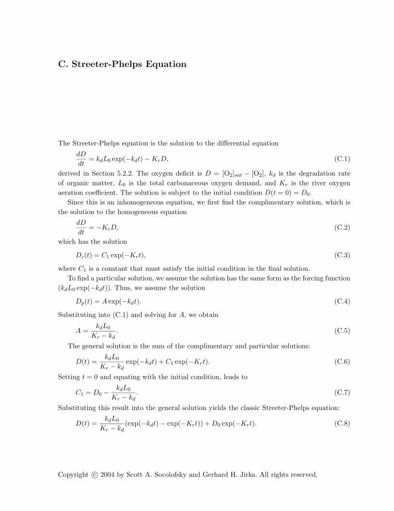
C. Streeter-Phelps Equation
The Streeter-Phelps equation is the solution to the differential equation
dD
dt= kdL0 exp(−kdt) − KrD, (C.1)
derived in Section 5.2.2. The oxygen deficit is D = [O2]sat − [O2], kd is the degradation rate
of organic matter, L0 is the total carbonaceous oxygen demand, and Kr is the river oxygen
aeration coefficient. The solution is subject to the initial condition D(t = 0) = D0.
Since this is an inhomogeneous equation, we first find the complimentary solution, which is
the solution to the homogeneous equation
dD
dt= −KrD, (C.2)
which has the solution
Dc(t) = C1 exp(−Krt), (C.3)
where C1 is a constant that must satisfy the initial condition in the final solution.
To find a particular solution, we assume the solution has the same form as the forcing function
(kdL0 exp(−kdt)). Thus, we assume the solution
Dp(t) = A exp(−kdt). (C.4)
Substituting into (C.1) and solving for A, we obtain
A =kdL0
Kr − kd. (C.5)
The general solution is the sum of the complimentary and particular solutions:
D(t) =kdL0
Kr − kdexp(−kdt) + C1 exp(−Krt). (C.6)
Setting t = 0 and equating with the initial condition, leads to
C1 = D0 −kdL0
Kr − kd. (C.7)
Substituting this result into the general solution yields the classic Streeter-Phelps equation:
D(t) =kdL0
Kr − kd(exp(−kdt) − exp(−Krt)) + D0 exp(−Krt). (C.8)
Copyright c© 2004 by Scott A. Socolofsky and Gerhard H. Jirka. All rights reserved.

156 C. Streeter-Phelps Equation

D. Common Water Quality Models
In this appendix we introduce a few of the common models used in water quality analysis. This
is by no means a complete list, but does provide a starting point from which to work. Much
of the text in this appendix was copied from the internet home pages describing each of the
models. The web page1 for this course provides links to each of these models in the web.
D.1 One-dimensional models
One-dimensional models are most commonly used in rivers, but can also be used in special cases
in estuaries and lakes with large length-to-width ratios. Accept for the ATV model, these models
are publicly available free of charge, and most can be downloaded over the internet. The list of
models below progresses from steady-state models, to dynamic tanks-in-series models, to fully-
dynamic numerical models. Refer to Chapter 7 for an introduction to water quality modeling
and its methodology.
D.1.1 QUAL2E: Enhanced stream water quality model
The qual2e series of models has a long history in stream water quality modeling. It was pri-
marily developed by the U.S. Environmental Protection Agency (EPA) in the early 1970s. Since,
it has gained a broad user base, including applications outside the U.S. in Europe, Asia, and
South and Central America.
The Enhanced Stream Water Quality Model (qual2e) is applicable to well mixed, dendritic
streams. It simulates the major reactions of nutrient cycles, algal production, benthic and car-
bonaceous demand, atmospheric reaeration and their effects on the dissolved oxygen balance.
It can predict up to 15 water quality constituent concentrations. It is intended as a water qual-
ity planning tool for developing total maximum daily loads (TMDLs) and can also be used in
conjunction with field sampling for identifying the magnitude and quality characteristics of non-
point sources. By operating the model dynamically, the user can study diurnal dissolved oxygen
variations and algal growth. However, the effects of dynamic forcing functions, such as headwa-
ter flows or point source loads, cannot be modeled with qual2e. Qual2e-u is an enhancement
allowing users to perform three types of uncertainty analyses: sensitivity analysis, first-order
error analysis, and Monte Carlo simulation.
1 http://ceprofs.tamu.edu/ssocolofsky/CVEN489/Book/Book.htm
Copyright c© 2004 by Scott A. Socolofsky and Gerhard H. Jirka. All rights reserved.

158 D. Common Water Quality Models
The model only simulates steady-state streamflow and contaminant loading conditions; the
reference to dynamic modeling above refers only to water quality forcing functions of climatologic
variables (air temperature, solar radiation, among others). The transport scheme in the model
is the implicit backward-difference finite difference method.
D.1.2 HSPF: Hydrological Simulation Program–FORTRAN
Developed in the late 1970s by the EPA, hspf is a union between the Stanford Watershed
Model, an advanced, continuous-simulation, process-oriented hydrologic model, and several wa-
ter quality models developed by the EPA, including the Agricultural Runoff Model (arm) and
the NonPoint Source model (nps). The model is intended for both conventional and toxic organic
pollutants. Contaminant loads are either user-input point sources or nonpoint sources modeled
by build-up and wash-off parameterizations. It is the only comprehensive model of watershed
hydrology and water quality that allows the integrated simulation of land and soil contaminant
runoff processes with in-stream hydraulic and sediment-chemical interactions. However, make
no mistake: it is not a three-dimensional model.
An advantage of hspf is in its software development, which resulted in a complete data-
management tool. A disadvantage of hspf is its large data requirements, which include physical
data such as watershed data, river network discretization, soil types, geologic setting, vegetative
cover, towns, and other regional data, meteorologic data such as hourly data for precipitation,
solar radiation, air temperature, dew-point temperature, and wind speed and daily evapotran-
spiration. In addition, the model has a wealth of empirical calibration parameters that must be
determined from handbook values and by calibrating to field measurements.
The river transport model is a tanks-in-series model that uses flood routing via stage-
discharge relationships (which must be input by the user from external knowledge).
D.1.3 SWMM: Stormwater Management Model
In urban settings, where pressurized pipe flow in sewer systems is to be modeled, the EPA
model swmm is recommended. The swmm model is actually a package of models. In one mode,
it can function as a design model which undertakes detailed simulations of storm events, using
relatively short time steps and as much catchment and drainage system detail as necessary. In
another mode it can be used as a routine planning model for an overall assessment of the urban
runoff problems and proposed abatement options. The planning mode is typified by continuous
simulation for several years using long (e.g. hourly) time steps and minimum detail in the
catchment scheme. Like hspf, the model requires a great deal of input data (both physical and
meteorological).
The modular nature of Swmm allows it to simulate diverse situations. Both single-event
and continuous simulation can be performed on catchments having storm sewers, or combined
sewers and natural drainage, for prediction of flows, stages and pollutant concentrations. The
Extran Block solves complete dynamic flow routing equations (St. Venant equations) for accu-
rate simulation of backwater, looped connections, surcharging, and pressure flow. The modeler

D.1 One-dimensional models 159
can simulate all aspects of the urban hydrologic and quality cycles, including rainfall, snowmelt,
surface and subsurface runoff, flow routing through drainage networks, storage and treatment.
Statistical analyses can be performed on long-term precipitation data and on output from con-
tinuous simulation.
The strength of this model is in its hydrodynamics. The transport modules, which are also
quite flexible, use simple tanks-in-series formulation, and are not available in the Extran Block
(where the complete dynamic flow equations are solved).
D.1.4 DYRESM-WQ: Dynamic reservoir water quality model
The model dyresm-wq is a one-dimensional hydrodynamics model for predicting the vertical
distribution of temperature, salinity and density in lakes and reservoirs. It is assumed that the
water bodies comply with the one-dimensional approximation in that the destabilizing forcing
variables (wind, surface cooling, and plunging inflows) do not act over prolonged periods of time.
Dyresm-wq has been used for simulation periods extending from weeks to decades. Thus, the
model provides a means of predicting seasonal and inter-annual variation in lakes and reser-
voirs, as well as sensitivity testing to long term changes in environmental factors or watershed
properties.
Dyresm-wq can be run either in isolation, for hydrodynamic studies, or coupled to caedym
for investigations involving biological and chemical processes. The computational demands of
dyresm-wq are quite modest and multi-year simulations can be performed on PC platforms
under Windows operating systems. The code is written in modular fashion to support future
updates and improvements.
D.1.5 CE-QUAL-RIV1: A one-dimensional, dynamic flow and water quality model
for streams
Administered and developed by the U.S. Army Corps of Engineers, ce-qual-riv1, or more
commonly just riv1, is a fully dynamic (flow and water quality) one-dimensional model. The
hydrodynamic portion is computed first, solving the St. Venant equations using the four-point
implicit finite difference scheme. The hydrodynamic model does not allow for super-critical flow.
This can lead to problems for natural streams under low flow where steep river sections form
cataracts. Following the hydrodynamics, the transport equation is solved using an explicit two-
point, fourth-order accurate Holly-Preissman scheme. The Holly-Preissman scheme is a backward
method of characteristics; however, because the search routine in RIV1 for finding the feet of
the characteristic lines only searches the upstream segment, the Courant number restriction still
applies. The water quality model can predict variations in each of 12 state variables: temperature,
carbonaceous biochemical oxygen demand (CBOD), organic nitrogen, ammonia nitrogen, nitrate
+ nitrite nitrogen, dissolved oxygen, organic phosphorus, dissolved phosphates, algae, dissolved
iron, dissolved manganese, and coliform bacteria. In addition, the impacts of macrophytes can be
simulated. Because of the use of the characteristic method, numerical accuracy for the advection
of sharp gradients is preserved.

160 D. Common Water Quality Models
D.1.6 ATV Gewassergutemodell
The ATV Gewassergutemodell, also called the AVG (allgemein verfugbares Gewassergutemodell)
or in English the ATV water quality model, was developed in Germany as a new model to
bridge the problems (limitations) inherent in some of the models listed above. It is designed as
a series of building blocks, each building block to be implemented as needed. The first building
block is the hydrodynamic model, which solves the St. Venant equations for either the steady
or unsteady case. The remaining building blocks can be added to the hydraulics as needed,
including water temperature, conservative tracers, (C)BOD, phosphorus, nitrogen cycle, silicon,
algae, zooplankton, sediment/water exchange, suspended sediment transport, oxygen dynamics,
pH dynamics, heavy metals, and organic chemicals. The solution to the transport equation
uses the method of characteristics and does not have a Courant number constraint. Because of
the model’s modular design, simulations can be made as simple or as complicated as desired;
however, the numerical expense of the hydrodynamic routine should not be underestimated.
D.2 Two- and three-dimensional models
Two- and three-dimensional models are typically used in reservoirs, lakes, and estuaries. They
are almost exclusively finite element, finite volume, or finite difference. Because large water
bodies are generally stratified, they must simulate buoyancy effects; thus, the hydrodynamic
and transport equations are coupled. Because buoyancy effects are a major complication in
these models (and the subject of next semester) this section briefly summarizes each model
without discussing the details.
D.2.1 CORMIX: Cornell Mixing-Zone Model
Begun at Cornell and currently under continued development at the Oregon Graduate Institute,
the cormix system is a near-field model for the analysis, prediction, and design of aqueous toxic
or conventional pollutant discharges into diverse water bodies. Major emphasis is on computation
of plume geometry and dilution characteristics within a receiving water’s initial mixing zone so
that compliance with regulatory constraints can be judged. It also computes discharge plume
behavior at larger distances. The model has three modules: cormix1 for submerged single-point
discharges, cormix2 for submerged multi-port diffuser discharges, and cormix3 for buoyant
surface discharges. As implied by the title, the model predicts mixing (dilution) of the input
chemicals, but does not allow for interaction among multiple chemicals (though first-order decay
of a single species is implemented).
The model equations are based on jets and plumes, which traditionally are modeled using
integral equations. Integral equations rely on self-similarity to reduce the three-dimensional
equations to a one-dimensional ODE. The model then solves for the three-dimensional trajectory
of the plume centerline using the one-dimensional integral equations. Hydrodynamic conditions
(though allowed to be unsteady) must be supplied as input to the model.
D.2 Two- and three-dimensional models 161
D.2.2 WASP: Water Quality Analysis Simulation Program
The wasp system is a generalized framework for modeling contaminant fate and transport in
surface waters. The model does not solve a set of multi-dimensional dynamical equations, but
rather is based on the flexible compartment modeling approach. Wasp can be applied in one,
two, or three dimensions. Problems that have been studied using the wasp framework include
biochemical oxygen demand and dissolved oxygen dynamics, nutrients and eutrophication, bac-
terial contamination, and organic chemical and heavy metal contamination.
Because wasp in an EPA model, input and output linkages also have been provided to other
stand-alone models. Flows and volumes predicted by the link-node hydrodynamic model dynhyd
can be read and used by wasp. Loading files from przm and hspf can be reformatted and read
by wasp. Toxicant concentrations predicted by toxi can be read and used by both the wasp
Food Chain Model and the fish bioaccumulation model fgets.
A body of water is represented in WASP as a series of computational elements or segments.
Environmental properties and chemical concentrations are modeled as spatially constant within
segments. Segment volumes and type (surface water, subsurface water, surface benthic, subsur-
face benthic) must be specified, along with hydraulic coefficients for riverine networks.
D.2.3 POM: Princeton ocean model
Pom is the precursor to ecom-si (see the next section), and was developed in the late 1970s. It is
a fully three-dimensional hydrodynamic numerical model, designed to predict ocean circulation.
The pom model is freely available to non-commercial applications.
The pom model contains an imbedded second moment turbulence closure sub-model to pro-
vide vertical mixing coefficients. It is a sigma coordinate model in that the vertical coordinate is
scaled on the water column depth. The horizontal grid uses curvilinear orthogonal coordinates.
The horizontal time differencing is explicit whereas the vertical differencing is implicit. The lat-
ter eliminates time constraints for the vertical coordinate and permits the use of fine vertical
resolution in the surface and bottom boundary layers. The model has a free surface and a split
time step. The external mode portion of the model is two-dimensional and uses a short time step.
The internal mode is three-dimensional and uses a long time step. Complete thermodynamics
have been implemented.
D.2.4 ECOM-si: Estuarine, coastal and ocean model
Ecom-si is a three-dimensional ocean circulation model developed principally by Alan Blumberg
of HydroQual. It is similar to the pom model, but incorporates a semi-implicit scheme for solving
the gravity wave so that the need for separate barotropic (external) and baroclinic (internal)
time steps is eliminated. The ecom-si model is not freely available, but must be obtained through
HydroQual.
Ecom-si includes a free surface, nonlinear advective terms, coupled density and velocity fields,
river runoff, heating and cooling of the sea surface, a 2.5 level turbulence closure scheme to

162 D. Common Water Quality Models
represent vertical mixing, and is designed to easily allow “realistic” simulations. In addition, the
combination of orthogonal curvilinear coordinates in the horizontal plane and sigma-coordinates
in the vertical dimension allows grid refinement in regions of interest without sacrificing the
well-known characteristics of Cartesian grid schemes. For water quality modeling, both pom
and ecom-si must be combined with a transport model.
Glossary 163
Glossary
adjacent [angrenzend o. benachbart ]:
Next to, nearby, or having a common endpoint or border.
advection [Advection]:
Transported by an imposed ambient current, as in a river or coastal waters.
ambient (fluid) [umgebend(es Fluid)]:
Ambient means “existing or present on all sides.” Ambient fluid is the fluid surrounding the
region of interest.
application [Anwendung ]:
An act of putting to use new techniques. A use to which something is put.
approach [Vorgehensweise]:
In science: a methodology applied to solve a problem.
assumption [Annahme]:
A fact or statement (as in a propostition, axiom, postulate, or notion) that is taken for
granted (assumed).
average [Durchschnitt ]:
A single value (as a mean, mode, or median) that summarizes or represents the general
significance of a set of unequal values.
boundary condition [Randbedingung ]:
A constraint applied to a differential equation at a physical location (boundary) in space.
buoyancy [Auftrieb]:
The tendency of a body to float or to rise when submerged in a fluid; the power of a fluid to
exert an upward force on a body placed in it, also, the upward force exerted on the body.
coherent [zusammenhangend o. kohrent ]:
Ordered of integrated in way that produces an interdependence.
control volume [Kontrollvolumen]:
The three-dimensional region defined by the boundaries of a system. Usually, a differential
element used to derive conservation laws.
convection [Konvektion]:
Vertical transport induced by hydrostatic instability, such as the flow over a heated plate,
or below a chilled water surface in a lake.
current [Stromung ]:
The part of a fluid body (such as air or water) moving continuously in a certain direction.
decay [Abbau o. Zerfall ]:
To decrease gradually in quantity, activity, or force.
density [Dichte]:
The mass of a unit volume.
derivation [Ableitung o. Herleitung ]:
The act or processes of forming a physical relationship from basic, accepted relationships.

164 Glossary
diffusion (molecular) [Diffusion (molekulare)]:
The scattering of particles by random molecular motions, which may be described by Fick’s
law and the classical diffusion equation.
diffusion (turbulent) [Diffusion (turbulente)]:
The random scattering of particles by turbulent motion, considered roughly analogous to
molecular diffusion, but with eddy diffusion coefficients (which are much larger than molec-
ular diffusion coefficients).
dilution [Verdunnung ]:
The act of reducing the strength, or concentration by adding more liquid.
discharge [Abfluß ]:
A flow, generally of contaminants, that is emitted into the environment, usually from a
localized source.
dispersion [Dispersion]:
The scattering of particles or a cloud of contaminants by the combined effects of shear and
transverse diffusion.
dissolve [losen]:
To cause to pass into solution.
droplets [Tropfchen]:
Small drops (as of a liquid), such as rain drops, drops of oil, and others. The liquid-phase
version of a gas bubble.
dye [Farbstoff ]:
A soluble or insoluble coloring matter.
eddy [Wirbel ]:
A current of water or air running contrary to the main current. In turbulent flow, especially,
a circular current or current with vorticity.
effluent [Ausfluß o. ausfließend ]:
The fluid flowing out from a discharge.
entrainment [Einmischung ]:
To draw in and transport (as solid particles or ambient fluid) by the flow of a fluid.
environmental impact statement [Umweltvertraglichkeitsstudie]:
Legal document reporting the projected positive and negative results to the environment of
a proposed engineering project.
equation [Gleichung ]:
A mathematical statement of equality or inequality.
estuary [Flußmundung o. Meeresbucht o. Astuar ]:
The a tidal region where fresh water (from continental sources) mixes with ocean water.
The estuary is generally defined up to the point where salt concentrations equal the ambient
ocean salinity.
evaporation [Evaporation]:
The transport of water vapor from a water or soil surface to the atmosphere.

Glossary 165
fluctuation [Schwankung ]:
A shirt back and forth uncertainly, or to ebb and flow in waves.
gauge (water gauge) [Meßgerat (Wasserstandsanzeiger)]:
An instrument with a graduated scale or dial for measuring or indicating quantity.
impact [Auswirkung o. Einfluß ]:
The changes, both positive and negative, on a natural system due to an external influence
(as an engineering project).
inertia [Tragheit ]:
a property of matter by which it remains at rest or in uniform motion in the same straight
line unless acted upon by some external force
initial condition [Anfangsbedingung ]:
A constraint applied to a differential equation at a physical moment in time (generally at
t = 0).
interface [Grenzflache]:
The boundary between two fluids.
jet [Strahl ]:
A momentum-driven boundary-layer flow. A usually forceful stream of fluid (as water or gas)
discharged from a narrow opening or a nozzle.
manifold [Verteiler- bzw. Sammelrohr ]:
A pipe fitting with several lateral outlets.
mean [Mittel ]:
See average.
mixing [Mischung ]:
Diffusion or dispersion as described above; turbulent diffusion in buoyant jets and plumes;
any process which causes one parcel of water to be mingled with or diluted by another.
momentum [Impuls]:
A property of a moving body that the body has by virtue of its mass and motion and that
is equal to the product of the body’s mass and velocity.
nozzle [Duse]:
A short tube with a taper or constriction used (as on a hose) to speed up or direct a flow of
fluid.
order of magnitude [Großenordnung ]:
A range of magnitude extending from some value to ten times that value.
orifice [Duse o. Offnung o. Mundung ]:
An opening (as a vent, mouth, or hole) through which something may pass.
particle entrainment [Teilcheneinmischen]:
The picking up of particles, such as sand or organic detritus, from the bed of a water body
by turbulent flow past the bed.
particle settling [Teilchenabsetzen]:
The sinking (or rising) of particles having densities different from the ambient fluid, such

166 Glossary
as sand grains or dead plankton. (In lakes and oceans the latter may be the dominant
mechanism for downward transport of nutrients, often all the way to the bottom.)
persistent [bestandig ]:
Existing for a long or longer than usual time or continuously; continuing without change in
function or structure. Also, degraded only slowly by the environment (as persistent contam-
inants).
plume [Fahne]:
A buoyancy-driven boundary-layer flow. A stream of fluid (as water or gas) with density
different from the ambient, recieving fluid, discharged from a narrow opening or nozzle, or
the fluid flow resultant from a discharge of heat.
plunge [eintauchen]:
To cause to penetrate or enter quickly and forcibly into something. To descend or dip sud-
denly.
pollutant [Schmutzstoff ]:
A substance that makes physically impure or unclean. To contaminant especially with man-
made waste.
porous media flow [Stromung in porosem Medium]:
Groundwater flow. Flow through a solid matrix containing many interconnected pores or
cavities (voids).
port [Offnung ]:
An opening (as in a diffuser manifold) for intake or exhaust of a fluid. See also orifice.
precipitation [Niederschlag ]:
A deposit on the earth of hail, mist, rain, sleet, or snow. Also refers to the quantity of water
deposited.
probability [Wahrscheinlichkeit ]:
The chance that a given event will occur. The branch of mathematics concerned with the
study of probabilities.
radiation [Strahlung ]:
The flux of radiant energy, such as at a water surface.
random [Zufall ]:
Without a definite aim, direction, rule, or method; lacking a definite plan, purpose, or pat-
tern.
residual [Rest ]:
The remaining product or substance.
salinity [Salzgehalt ]:
A measure of the salt content of seawater, specifically, the ratio of the mass of dissolved salts
to the total mass of water and salt.
saturated [gesattigt ]:
Being a solution that is unable to absorb or dissolve any more of a solute at a given temper-
ature and pressure.

Glossary 167
sewage [Abwasser ]:
The raw refuse liquids or waste matter carried off by sewers.
sewage treatment plant [Klarwerk o. Klaranlage]:
The facility where sewage is prepared (cleaned) before releasing it into the environment as
effluent.
shear flow [Scherstromung ]:
The advection of fluid at different velocities at different positions; this may be simply the
normal velocity profile for a turbulent flow where the water flows faster with increasing
elevation above the bed of the stream; or shear may be the changes in both magnitude and
direction of the velocity vector with depth in complex flows such as in estuaries or coastal
waters.
shear stress [Scherspannung ]:
A force exerted from one fluid layer to another, due to differences in their velocity, that tends
to pull on, push against, or compress or twist the fluid body.
soluble [loslich]:
The property of being able to be dissolved in a fluid (the dissolving fluid is referred to as
the solute).
source [Quelle]:
The location and flux of a flow (usually of a contaminant or substance of interest).
spatial [raumlich]:
Relating to, occupying, or having the character of space. A spatial distribution is the de-
scription of the variation of a quantity in space. Compare with temporal.
standard deviation [Standardabweichung ]:
A statistical quantity describing the degree of spread of a distribution. Defined as the square
root of the variance. The variance is the mean of the squared deviations from the mean.
steady [stationar ]:
In steady state, or unchanging. The mathematical representation is that the time derivative
is zero.
stratification [Schichtung ]:
The property of being stratified. An organization of a fluid body based on density. The most
common form of density stratification is the stable form, where density decreases as height
increases.
submerged [abgetaucht ]:
The state of being emersed within a fluid (as being underwater).
temporal [zeitlich]:
Relating to, occupying, or having the character of time. A temporal distribution is the
description of the variation of a quantity in time. Compare with spatial.
tracer [Tracer ]:
Any conservative (non-transforming) substance that moves exactly with the fluid (i.e. does
not move relative to the fluid).

168 Glossary
transformation [Transformation]:
The changing of a chemical substance into another chemical substance, usually accompa-
nied by the loss of the original substance (i.e. carbon dioxide transformed into oxygen by
photosynthesis).
transport [Transport ]:
The movement of a parcel of water or tracer by advection, diffusion, or mixing.
unsteady [instationar ]:
Changing, or developing in time. The mathematical representation is that the time derivative
is not zero. See also steady.
volatile [fluchtig ]:
Readily vaporizable at a relatively low temperature.
vortex [Wirbel ]:
See eddy.
vorticity [Wirbelstarke]:
A vector measure of the local rotation in a fluid flow.
wake [Nachlaufwirbel ]:
The region of velocity deficit behind an object held stationary relative to an ambient fluid
flow.
wastewater [Abwasser ]:
An effluent flow of fluid no longer of use. See also sewage.
References
Acheson, D. J. (1990), Elementary Fluid Dynamics, Clarendon Press, Oxford.ASCE & WPCF (1992), ‘Design and construction of urban stormwater management systems’.Batchelor, G. K. (1967), An introduction to fluid dynamics, Cambridge University Press, Cambridge, England.Boyd, J. P. (1989), Lecture Notes in Engineering 49: Chebyshev and Fourier Spectral Methods, Springer Verlag,
Heidelberg, Germany.Brooks, N. H. (1960), Diffusion of sewage effluent in an ocean current, in ‘Proc. 1st Int. Conf. Waste Disposal
Mar. Environ.’, Pergamon Press, Oxford, pp. 246–267.Cramer, H. E. (1959), Am. Ind. Hyg. Assoc. J. 20, 183.Csanady, G. T. (1973), Turbulent Diffusion in the Environment, Geophysical and Astrophysics Monographs, D.
Reidel Publishing Company, Dordrecht, Holland.Deng, Z.-Q., Singh, V. P. & Bengtsson, L. (2001), ‘Longitudinal dispersion coefficient in straight rivers’, J. Hydr.
Engrg. 127(11), 919–927.Fedorovich, E. (1999), Course notes: Atmospheric diffusion and dispersion, Technical report, European Graduate
School of Hydraulics, Short course on Environmental Fluid Mechanics: Theory, Experiments, Applications,IAHR-EGH, Karlsruhe, Germany.
Fischer, H. B., List, E. G., Koh, R. C. Y., Imberger, J. & Brooks, N. H. (1979), Mixing in Inland and Coastal
Waters, Academic Press, New York, NY.Garratt, J. R. (1992), The atmospheric boundary layer, Cambridge Atmospheric and Space Science Series, Cam-
bridge University Press, Cambridge, England.Gschwend, P. S. (1987), Modeling the benthos-water column exchange of hydrophobic chemicals, Technical Report
unkn., USEPA, Environmental Research Lab., Wash., D.C.Kaimal, J. C. & Finnigan, J. J. (1994), Atmospheric Boundary Layer flows: Their structure and measurement,
Oxford University Press, Inc., New York.Lumley, J. L. & Panofsky, H. A. (1964), The Structure of Atmospheric Turbulence, Interscience Publishers, New
York.Mathieu, J. & Scott, J. (2000), An introduction to turbulent flow, Cambridge University Press, Cambridge.Mei, C. C. (1997), Mathematical Analysis in Engineering, Cambridge University Press, Cambridge, England.Nepf, H. M. (1995), ‘Course notes and problem sets’, MIT Course 1.77: Water Quality Control .Okubo & Karweit (1969), ‘Title’, Journal p. Pages.Panofsky, H. A. (1967), A survey of current throught on wind properties relevant for diffusion in the lowest 100 m,
in ‘Symp. Atm. Turb. Diffusion’, Sandia Laboratories, Albuquerque, NM, pp. 47–58.Pasquill, F. (1962), Atmospheric Diffusion, D. van Nostrand Co. Ltd., New York.Pope, S. B. (2000), Turbulent Flows, Cambridge University Press, Cambridge.Reynolds, O. (1883), Phil. Trans. R. Soc. Lond. 174, 935–982.Rutherford, J. C. (1994), River Mixing, John Wiley & Sons, Chichester, England.Smart, P. L. & Laidlay, I. M. S. (1977), ‘An evaluation of some fluorescent dyes for water tracing’, Wat. Res. Res.
13(1), 15–33.Smith (1957), ‘Title’, Journal p. Pages.Sutton, O. G. (1932), Proc. Roy. Soc. London A 135, 143.Sutton, O. G. (1953), Micrometeorology, McGraw-Hill Book Co., New York.Taylor, G. I. (1921), ‘Diffusion by continuous movements’, Proc. London Math. Soc., Ser. 2 20, 196–212.Thomann, R. V. & Mueller, J. A. (1987), Principles of Surface Water Quality Modeling and Control, Harper &
Row, Publishers, New York.Walters (1962), ‘Title’, Journal p. Pages.
Copyright c© 2004 by Scott A. Socolofsky and Gerhard H. Jirka. All rights reserved.

170 References

Index
e-folding time, 85
adsorption, 107advection, 29– advective-diffusion equation, see diffusionaeration rate, 105atmosphere, 113– APBL, see boundary layer– atmospheric boundary layer, see boundary layer– atmospheric turbulence, 113– capping inversion, see capping inversion
biochemical oxygen demand (BOD), 105biodegradation, 102biological transformation, see transformationbioturbation, 106boundaries– exchange, see interfaces– flux, see interfaces– no-flux, 37boundary layer, 95– atmospheric boundary layer (APBL), 113, 114– concentration boundary layer, 97– turbulent boundary layer, 114Buckingham π theorem, see dimensional analysis
calibrate, 129calibration, 137capping inversion, 114chain rule, 16, 31, 62characteristic scales, 33chemical transformation, see transformationconservation equations– mass, 11, 137conservative system, 81conservative tracer, see tracercontinuity equation, see conservation equationscontinuously-stirred tank reactor, 131coordinate transformation, 31crossflow, see currentscurrents, 163
delta function, 15desorption, 107diffusion, 8, 29– advective-reacting diffusion equation, 89
– advective diffusion equation, 29– diffusion coefficient, 10, 12– diffusion equation, 11– diffusive transport, see transport– Fick’s law, 10– Fickian diffusion, 9, 10dimensional analysis, 7– Buckingham π-theorem, 7– dimensionless variable, 7– similarity solution, see similarity solutiondispersion, 59– longitudinal dispersion coefficient, 64, 71dissipation, ε, see turbulencedistribution coefficient, 108dye study, 67– breakthrough curve, 71
environmental fluid mechanics, 1erosion, 106error function, erf(u), 35Eulerian reference frame, 53, 135examples– arsenic contamination, 20– fish nursery, 41explicit, 135
far field, 121fetch, 115Fick’s law, see diffusionfilm renewal model, 98– renewal frequency, 99finite difference, 135finite element, 135finite volume, 135flocculation, 105flux boundary condition, 91frame of reference, 29, 34
gas exchange, 95, 101– gas transfer coefficient, 102
half-life, 82, 83, 85, 92heterogeneous reaction, 81, 82, 90, 95homogeneous reaction, 81, 82, 89, 95
image source, 39

172 Index
implicit, 135inertial sub-layer (ISL), 115interface, 95– air-water, 95– boundary fluxes, 95– exchange, 95– sediment-water, 95, 104
Lagrangian reference frame, 53, 135laminar flow, 52Langmuir isotherm, 108Lewis-Whitman model, 98log-velocity profile, 57, 115longitudinal dispersion, see dispersion
Marriot bottle, 69mass conservation, see conservation equationsmixture, 82model, 125momentum conservation, see conservation equationsmulti-phase, 82
near field, 121numerical diffusion, 134
particle entrainment, see entrainmentparticle settling, see settlingpartition coefficient, 108passive tracer, see tracerPeclet number, 33, 128photosynthesis, 83physical transformation, see transformationplug-flow reactor, 130porosity, 104Prandtl layer, 115products, 83
radioactive decay, 82rate law, see transformationreactants, 83reaction, see transformationreactive, 81respiration, 83Reynolds decomposition, see turbulence
scale analysis, 63sedimentation, 105settling, 82, 105settling velocity, see slip velocityshear flow, 59shear velocity, 56similarity solution, 14, 16, 18
– self similarity, 20single-phase, 82sink, 81, 82, 89slip velocity, 104solutions– fixed concentration, 36– spatial concentration distribution, 34source, 81, 82, 89stability, 117– neutral, 117– stable, 117– unstable, 117standard deviation, 19Streeter-Phelps equation, 102, 104superposition, 29, 34
tanks-in-series model, 132Taylor series expansion, 30Taylor series expansion, 13terminal velocity, see slip velocitytracer, 12transfer velocity, 97, 99transformation, 81, 95– e-folding time, see e-folding time– biological, 81, 83– chemical, 81, 82– first-order, 81, 82, 85– half-life, see half-life– higher-order, 81, 88– kinetics, 81, 83– physical, 81, 82– rate law, 84– second-order, 81, 86transport– advective transport, see advection– diffusive transport, 9, 22turbulence, 51, 52– dissipation, ε, 53– energy cascade, 53– fluctuating velocity, 54– homogeneous, 53– integral scales, 54– production, 53– root mean square velocity, urms, 54– turbulence intensity, 116
validate, 129validation, 137viscous sub-layer (VSL), 115
wastewater treatment plant, 81, 91