cv45 geotechnical engineering 1 module 1nptel.vtu.ac.in/econtent/web/cv/15cv45/pdf/module1.pdf ·...
TRANSCRIPT

CV45: Lecture Notes for Module 1 by Prof. S.K. Prasad 1
CV45 Geotechnical Engineering – 1
Module 1
Introduction, Phase Diagrams, Index Properties & Soil
Classification
Dr. S.K. Prasad Professor of Civil Engineering
Sri Jayachamarajendra College of Engineering Mysuru 570 006
Email: [email protected]
February 2018

CV45: Lecture Notes for Module 1 by Prof. S.K. Prasad 2
CV45 Geotechnical Engineering – 1
Module 1
Syllabus
Introduction
Origin & Formation of Soil, Phase Diagram, Phase relationships, Definitions and their
relationships.
Determination of Index Properties
Specific Gravity, Water Content, Insitu Density, Particle size analysis (Sieve Analysis and
Sedimentation Analysis), Atterberg’s Limits, Consistency Indicies, Relative Density Activity
of Clay
Soil Classification
Plasticity Chart, Unified and BIS Soil Classification
ACKNOWLEDGEMENT
A number of pictures and some materials have been downloaded from internet over years. I
wish to acknowledge all those who have indirectly contributed. The lecture material is only
intended to help the students. Hence, I do not claim anything as original.
INTRODUCTION
1.1 Geotechnical Engineering – Why?
1. We are unable to build castles in air (yet) !
2. Almost every structure is either built on or built in or built using soil or rock.
3. Mechanics of Soils and Rocks is the basis of Geotechnical Engineering
4. Geotechnical engineering problems involve:
– Strength
– Stability
– Deformation
– Water flow
Soil is an un-cemented aggregate of mineral grains and decayed organic matter (solid
particles) with liquid and gas in the empty space between the solid particles formed by
weathering of rocks in the top surface of earth crust. Fig. 1 represents a portion of soil mass
comprising of solid particles and void space. Void space is made up of liquid (water) and/or
gas (air).

CV45: Lecture Notes for Module 1 by Prof. S.K. Prasad 3
Fig. 1 : Soil mass, a conglomeration of solid particles and void space
Soil is an important construction material that is
1. Oldest.
2. Cheap or available free of cost many a times.
3. Most complex, yet having interesting properties.
4. Modified to suit the requirements, many a times.
Soil is used
1. to manufacture Bricks, Tiles or Earthenware.
2. as foundation material.
3. to construct dams and embankments.
4. to fill hollow zones behind retaining walls, low lying areas etc.
5. to construct landfills and other environmental protection systems
1.2 Why soil is complex?
The following properties of soil make it perhaps the most complex construction material. 1. Porous
2. Polyphasic
3. Permeable
4. Particulate
5. Heterogeneous
6. Anisotropic
7. Non-Linear
8. Pressure Level Dependent
9. Strain Level Dependent
10. Strain Rate Dependent
11. Temperature Dependent
12. Undergoes volume change in shear
Yet, soil possesses some Interesting properties that relate with human beings, namely,
1. Colorful
2. Sensitive

CV45: Lecture Notes for Module 1 by Prof. S.K. Prasad 4
3. Possesses Memory
4. Changes its properties with time
1.3 What is Geotechnical Engineering?
Geotechnical Engineering is an integration of Physics, Earth Science, Solid Mechanics,
Geology and Hydrogeology. The basic science of Geotechnical Engineering is called Soil
Mechanics. Geotechnical Engineering provides the theoretical basis for describing the
mechanical behaviour of earth materials. It involves application of theory of soil mechanics
to a variety of field problems. For most other engineering disciplines, the material
properties are well-defined or can be controlled. But, in Geotechnical Engineering, material
properties are highly variable and difficult to measure with a reasonable degree of accuracy. Geotechnical Engineering is among the younger branches of Civil Engineering. Yet, it has
evolved over centuries.
1. Geotechnical Engineering is probably one of the most challenging engineering disciplines.
2. For a geotechnical engineer, no two days at work are going to be similar. 3. Geotechnical engineering expertise is required in a vast variety of disciplines that
includes the oil and offshore industry. 4. Being a relatively new discipline, there is ample scope for innovation. 5. For a geotechnical engineer, achieving job satisfaction is never a problem. 6. Material properties must be measured for each new construction site. 7. Remember that geotechnical engineers deal with natural materials and there can be
no quality control. 8. Ground consists of innumerable variety of particle sizes and minerals. 9. To make matter worse, engineering properties of earth materials are strongly
influenced by their past geological history that is normally unknown. Climatic conditions also influence these properties.
1.4 Sub-branches in Geotechnical Engineering
The following are the sub-branches of Geotechnical Engineering.
1. Foundation Engineering
2. Deep Excavation
3. Tunneling
4. Earth Pressure and Retaining Structures
5. Earth embankments
6. Stability of Slopes
7. Environmental Geotechniques
8. Earthquake Geotechnical Engineering
9. Ground Improvement technique
10. Rock Mechanics
11. Engineering geology

CV45: Lecture Notes for Module 1 by Prof. S.K. Prasad 5
Fig. 2 represents the family of Geotechnical engineering.
Fig. 2 : Family of Geotechnical Engineering
1.5 Distinctions between Fine and Coarse Grained Soils
Soil can be broadly classified in to two types, namely Fine grained soil and coarse
grained soil based on the size, shape and behaviour. Table 1 provides the important
distinctions.
Table 1 : Distinctions between Fine grained soil and coarse grained soil
Fine Grained Soil Coarse Grained Soil
Size of particle is less than 75 microns Size of particle is mores than 75 microns
Silt & Clay belong to this group Sand, Gravel, Cobble, Boulder etc. belong to this group
Properties are influenced by surface area Properties are influenced by gravity
Attraction and bonding between particles enable strength
Dense packing, particle to particle contact enable strength
Mostly plate-like Mostly round, sub-round, angular
Void ratio & water content can be very high Void ratio & water content can not be very high
Possess consistency (liquid, plastic & shrinkage) limits
Consistency (liquid, plastic & shrinkage) limits are absent
Possess Cohesion Possess Angle of Internal friction
1.6 Soil formation, a geologic Cycle
Soil is formed from rock due to erosion and weathering action. Igneous rock is the basic rock
formed from the crystallization of molten magma. This rock is formed either inside the earth
or on the surface. These rocks undergo metamorphism under high temperature and
pressure to form Metamorphic rocks. Both Igneous and metamorphic rocks are converted in
Geotechnical
Engg.
Foundation
Engg
Deep
Excavations
Tunneling
Retaining
Structures
Slopes
Embankments
Environmental
Geotechnics
Earthquake
Geotechnical
Engg.

CV45: Lecture Notes for Module 1 by Prof. S.K. Prasad 6
to sedimentary rocks due to transportation to different locations by the agencies such as
wind, water etc. Finally, near the surface millions of years of erosion and weathering
converts rocks in to soil.
Fig. 3 : Geological Cycle of Soil

CV45: Lecture Notes for Module 1 by Prof. S.K. Prasad 7
PHASE SYSTEM
1.7 Soil Mass, a three phase system
If you take a lump of soil in hand, it looks like the one in Fig. 4. When seen through
microscope, you can observe that the soil mass is made up of innumerable number of soil
particles in contact with each other. Each particle can have different shapes and sizes. In
between particles, there will be voids which can be filled with air and / or water. Hence, soil
mass comprises of solid particles of soil, water and air. The three of them form a three phase
system. However, it is very difficult to consider their interaction precisely. Hence, to
simplify the understanding, the three phases are divided in to three volumes by combining all
materials belonging to one phase. They are further explained on volume and weight basis. We
call this as three phase system.
A typical soil mass Idealisation as three phase system
Fig. 4: Soil mass idealized as three phase system

CV45: Lecture Notes for Module 1 by Prof. S.K. Prasad 8
W = Weight
V = Volume
s = Soil grains
w = Water
a = Air
v = Voids
Basic terminologies in a three phase system of soil mass
Conversion from three to two phase system
Fig. 5 : Soil mass as three phase system
1.8 Basic Definitions
The following are the basic definitions of soil.
1. Water Content (ω)
2. Void Ratio (e)
3. Porosity (n)
4. Degree of Saturation (S)
5. Air content (Ac)
6. Percentage air voids (na)
7. Bulk Density (γb)

CV45: Lecture Notes for Module 1 by Prof. S.K. Prasad 9
8. Dry density (γd)
9. Density of soil solids (γs)
10. Saturated density (γsat)
11. Density of water (γω)
12. Submerged density (γsub)
13. Specific Gravity of Soil Solids (G)
14. Specific Gravity of Soil Mass (Gm)
15. Relative density (Dr)
Each of the above definition is defined with soil represented as three phase diagram.
1.8.1 Water Content (ω)
1. It is defined as ratio of weight of water to weight of solids.
2. It is also called Moisture Content.
3. It has no unit. It is expressed in percentage or decimals (for calculation purpose).
4. It indicates the amount of water present in the voids in comparison with weight of
solids.
5. In dry soil, water content ω = 0.
6. Clayey soil may possess very large water content leading to unfavourable situation.
7. Water content of soil mass changes with season, being close to zero in summer and
maximum during rainy season.
8. It represents the amount of water present in soil mass. In dry soil, water content ω = 0
9. Higher the water content, greater will be the vulnerability, especially in clayey soil.
1.8.2 Void Ratio (e)
1. It is defined as the ratio of volume of voids to volume of solids
2. It has no unit. It is normally expressed in decimals.
3. It indicates the amount of voids present in a soil mass in comparison with the
amount of solids.
4. Normally, void ratio of clayey soil will be large.
5. The more the void ratio, more loose will be the soil mass and hence, less strong and
less stiff.
6. It is not possible to determine void ratio in the laboratory. Hence, it is computed
from other properties.
CV45: Lecture Notes for Module 1 by Prof. S.K. Prasad 10
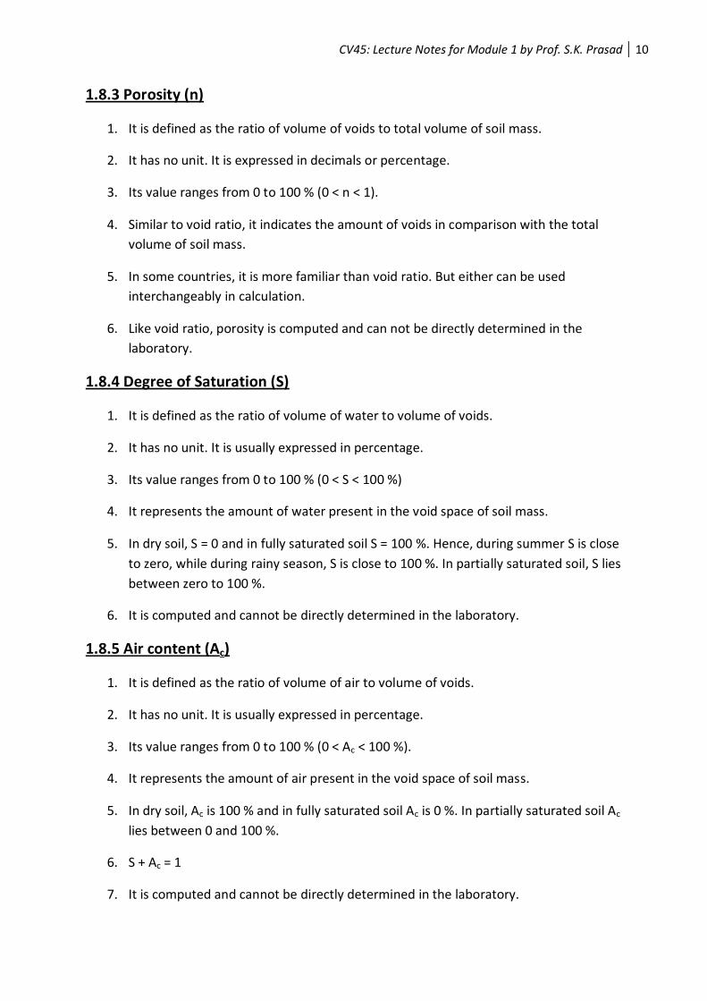
1.8.3 Porosity (n)
1. It is defined as the ratio of volume of voids to total volume of soil mass.
2. It has no unit. It is expressed in decimals or percentage.
3. Its value ranges from 0 to 100 % (0 < n < 1).
4. Similar to void ratio, it indicates the amount of voids in comparison with the total
volume of soil mass.
5. In some countries, it is more familiar than void ratio. But either can be used
interchangeably in calculation.
6. Like void ratio, porosity is computed and can not be directly determined in the
laboratory.
1.8.4 Degree of Saturation (S)
1. It is defined as the ratio of volume of water to volume of voids.
2. It has no unit. It is usually expressed in percentage.
3. Its value ranges from 0 to 100 % (0 < S < 100 %)
4. It represents the amount of water present in the void space of soil mass.
5. In dry soil, S = 0 and in fully saturated soil S = 100 %. Hence, during summer S is close
to zero, while during rainy season, S is close to 100 %. In partially saturated soil, S lies
between zero to 100 %.
6. It is computed and cannot be directly determined in the laboratory.
1.8.5 Air content (Ac)
1. It is defined as the ratio of volume of air to volume of voids.
2. It has no unit. It is usually expressed in percentage.
3. Its value ranges from 0 to 100 % (0 < Ac < 100 %).
4. It represents the amount of air present in the void space of soil mass.
5. In dry soil, Ac is 100 % and in fully saturated soil Ac is 0 %. In partially saturated soil Ac
lies between 0 and 100 %.
6. S + Ac = 1
7. It is computed and cannot be directly determined in the laboratory.

CV45: Lecture Notes for Module 1 by Prof. S.K. Prasad 11
1.8.6 Percentage air voids (na)
1. It is defined as the ratio of volume of air to total volume of soil mass.
2. It has no unit. It is expressed in percentage.
3. Its value ranges from zero to 100 % (0 < na < 100 %).
4. It represents the amount of air present in the total volume of soil mass.
5. Always na < Ac.
6. It is computed and can not be directly determined in the laboratory.
1.8.7 Bulk Density (γb)
1. It is defined as the ratio of total weight to total volume of soil mass.
2. In SI units, it is expressed as kN/m3.
3. Its value normally ranges from 12 to 24 kN/m3.
4. It includes the weights of air, water and solids as a function of total volume of soil
mass. It changes with season, being maximum during rainy season and minimum in
summer.
5. Bulk density of soil mass can be determined experimentally. It is therefore used to
compute other properties such as dry density and void ratio.
1.8.8 Dry density (γd)
1. It is defined as the ratio of weight of soil solids to total volume of soil mass.
2. In SI units, it is expressed as kN/m3.
3. Dry density will always be less than or equal to bulk density of soil mass.
4. Dry density is independent of season. Hence, it is used in many design calculations.
5. Knowing water content and bulk density, dry density can be computed.
1.8.9 Density of soil solids (γs)
1. It is defined as the ratio of weight of soil solids to volume of soil solids.
2. In SI units, it is expressed as kN/m3.
3. It is always greater than dry density of soil.

CV45: Lecture Notes for Module 1 by Prof. S.K. Prasad 12
4. It can not be determined experimentally. Hence, it is computed from other
parameters. It is used to calculate other properties such as specific gravity of soil
solids.
1.8.10 Saturated density (γsat)
1. It is defined as the ratio of total weight to total volume of soil mass when the soil is
fully saturated. Hence, it is the bulk density of soil mass when S = 1.
2. In SI units, it is expressed as kN/m3.
1.8.11 Density of water (γω)
1. It is defined as the ratio of weight of water to volume of water.
2. In SI units, it is expressed in kN/m3 and can be taken as 9.8 kN/m3.
3. It is used in computation of other quantities.
1.8.12 Submerged density (γsub)
1. It is defined as the net weight of weight per volume of soil mass in water.
2. In SI units, it is expressed as kN/m3.
3. It is equal to saturated density minus density of water.
4. satsub
5. It is also called buoyant density.
6. In saturated soil, water exerts upward pressure on soil. Net weight of soil particles
acting downward will be actual weight of soil minus weight of water.
1.8.13 Specific Gravity of Soil Solids (G)
1. It is defined as the weight of soil solids to weight of equal volume of water.
2. Hence, it is the ratio of density of soil solids to density of water.
3. It has no units and is expressed in decimals.
4. Normally, G of most soils varies from 2.6 to 2.75. Organic soils may have G up to 2.
5. G is determined in the laboratory and is used to compute other parameters such as
void ratio.
6. Many a times, specific gravity means G

CV45: Lecture Notes for Module 1 by Prof. S.K. Prasad 13
1.8.14 Specific Gravity of Soil Mass (Gm)
1. It is defined as the weight of soil mass to weight of equal volume of water.
2. It is also called Apparent Specific Gravity.
3. It has no units and is expressed in decimals.
4. Its magnitude is always smaller than that of G.
5. It is less commonly used in calculations.
1.8.15 Relative density (Dr)
1. It is also called Density Index.
2. It has no unit. It is expressed in percentage.
3. Dr ranges from 0 to 100 %.
4. It is applicable for coarse grained soil such as sand and gravel.
5. It indicates whether the insitu density of soil is close to loosest or densest state.
6. minmax
max
ee
eeDr
7. In terms of dry density, relative density is given as follows.
minmax
minmax
dd
dd
d
d
rD
8. When Dr = 1, soil in its densest state and when Dr = 0, soil is in its loosest state.
Table 2 : Influence of Relative density on Soil State
Relative Density (%) State of Soil
0 to 20 Very Loose
20 to 40 Loose
40 to 60 Medium dense
60 to 80 Dense
80 to 100 Very Dense

CV45: Lecture Notes for Module 1 by Prof. S.K. Prasad 14
1.9 Problems and Solutions related to Phase Diagram
Problem 1
A natural soil mass has a bulk density of 18 kN/m3 and water content of 8 %. Calculate the
amount of water required per cubic meter of soil to raise the water content to 18 %. What
will be the degree of saturation at this water content? Assume void ratio to be constant and
take G = 2.7. (July 2006) 8 Marks
Data
γb = 18 kN/m3
ω = 8 %
G = 2.7
γω = 9.8 kN/m3 (assumed)
3/67.161
mkNb
d
587.01d
Ge
V
Ws
d
Hence, for 1 m3 of soil mass, Ws = 16.67 kN
If ω = 8 %, weight of water = 0.08Ws = 1.33 kN
If ω = 18 %, weight of water = 0.18Ws = 3 kN
Hence, amount of water required per cu.m of soil = 3 – 1.33 = 1.67 kN = 167 lt.
%8.82828.0
S
SeG
Problem 2
How many cu.m of soil can be formed with void ratio of 0.5 from 100 m3 of soil having void
ratio of 0.7? (Jan 2006) 5 Marks
Data
e1 = 0.7
Vv1 = 0.7Vs
V1 = 100 m3 = Vv1 + Vs = 1.7 Vs
Vs = 58.82 m3
e2 = 0.5
Vv2 = 0.5Vs = 29.41 m3
V2 = Vv2 + Vs = 88.23 m3

CV45: Lecture Notes for Module 1 by Prof. S.K. Prasad 15
Problem 3
A dry soil has a void ratio of 0.65 and specific gravity is 2.8. Find its unit weight. Water is
added to the sample so that its degree of saturation is 55 % without any change in void
ratio. Determine the water content and unit weight. The sample is then submerged in
water. Determine the unit weight when the degree of saturation is 90 % and 100 %. (Jan
2008) 10 Marks
Data
e = 0.65
G = 2.8
γω= 9.8 kN/m3 (assumed)
3/63.161
mkNe
Gd
When S = 55 %, ω = 12.77 % 3/75.18)1( mkNdb
When S = 90 %, ω = 20.89 %
When S = 100 %, ω = 23.21 %
Problem 4
In an earth dam under construction, the bulk unit weight is 16.5 kN/m3 at water content 11
%. If the water content has to be increased to 15 %, compute the quantity of water to be
added per cu.m of soil. Assume no change in void ratio. Determine the degree of saturation
at this water content. Take G = 2.7. (Jan 2009)
10 Marks.
Data
γb =16.5 kN/m3
ω = 11 %
G = 2.7
γω= 9.8 kN/m3 (assumed)
3/86.141
mkNb
d
Wd = 14.86 kN per unit volume
Ww = 1.63 kN per unit volume
78.01d
Ge
%92.51e
GS

CV45: Lecture Notes for Module 1 by Prof. S.K. Prasad 16
Problem 5
An undisturbed specimen of clay was tested in a laboratory and the following results were
obtained. Weight = 2.1 N, Oven dry weight = 1.75 N. Specific Gravity of soil solids = 2.7.
What was the total volume of original undisturbed specimen assuming that the specimen
was 50 % saturated? (Model QP) 8 Marks
Data
W = 2.1 N
Ws = 1.75 N
Ww = 0.35 N
G = 2.7
S = 0.5
γω= 9.8 kN/m3 (assumed)
%20sW
W
08.1S
Ge
3/72.121
mkNe
Gd
72.121075.1 3
V
X
V
Ws
d
V = 0.1376 X10⁻³ m3
Problem 6
The maximum and minimum dry unit weights of sand determined in the laboratory are 21
kN/m3 and 16 kN/m3 respectively. If the relative density of sand is 60 %, determine the in-
situ porosity of the sand deposit. Take G = 2.65. (June 2008) 6 Marks
Data
Dr = 60 % =0.6
γdmax = 21 kN/m3
γdmin = 16 kN/m3
γd = 18.67 kN/m3
minmax
minmax
dd
dd
d
d
rD
78.01d
Ge
e
en
1 0.44

CV45: Lecture Notes for Module 1 by Prof. S.K. Prasad 17
Problem 7
For a soil in its natural state, void ratio, water content and specific gravity are respectively
0.8, 24 % and 2.68. Determine bulk density, dry density and degree of saturation. If the soil
is completely saturated by adding water, what would be its water content and saturated
density.
Data
e=0.8
ω = 0.24
G = 2.68
γω= 9.8 kN/m3 (assumed)
3/59.141
mkNe
Gd
3/09.18)1( mkNdb
%4.80e
GS
If S =1, ω =29.85 % 3/95.18)1( mkNdsat
Problem 8
In its natural condition, a soil sample has a mass of 22.9 N and a volume of 1.15 X 10⁻³ m3.
After being completely dried in the oven sample weighs 20.35 N. Find bulk density, water
content, void ratio, porosity, degree of saturation, air content, dry density and percentage
air voids.
Data
W = 22.9 N
V = 1.15 X 10⁻³ m3
Ws = 20.35 N
G = 2.7
γω= 9.8 kN/m3 (assumed)
3
3/91.19
1015.1
9.22mkN
XV
Wb
ω = 12.53 %
γd = 17.7 kN/m3
495.01d
Ge
e
en
10.331
%35.68
e
GS

CV45: Lecture Notes for Module 1 by Prof. S.K. Prasad 18
Ac = 1 – S = 31.65 %
G
Gna
d
1
)1(
na = 0.105
Problem 9
A moist sample of soil has a weight of 6.33 N and a volume of 300000 mm3 at a water
content of 11 %. Taking G = 2.68, determine e, S and na. Also determine water content at
which soil gets fully saturated. What will be the unit weight at saturation?
Data
W = 6.33 N
V = 3X105 mm3
G = 2.68
ω = 11%
γw = 9.8 kN/m3
3/1.21 mkNV
Wb
3/191
mkNbd
38.01d
Ge
%6.77e
GS
If S = 1, then %18.14G
e
3/69.21)1( mkNdsat
Problem
A sample of soil has a volume of 1X106 mm
3 and weighs 19 N. The water content of the soil
is 15% and G = 2.7. Find dry density, void ratio, degree of saturation and water content at
saturation. Take γw = 9.81 kN/m3
W = 19 N = 0.019 kN
V = 1X 106 mm
3 = 1X10
-3 m
3
γb = W/V = 19 kN/m3
If S = 1, then
3/52.161
mkNbd
60.01d
Ge
%5.67e
GS
%2.22G
e
CV45: Lecture Notes for Module 1 by Prof. S.K. Prasad 19
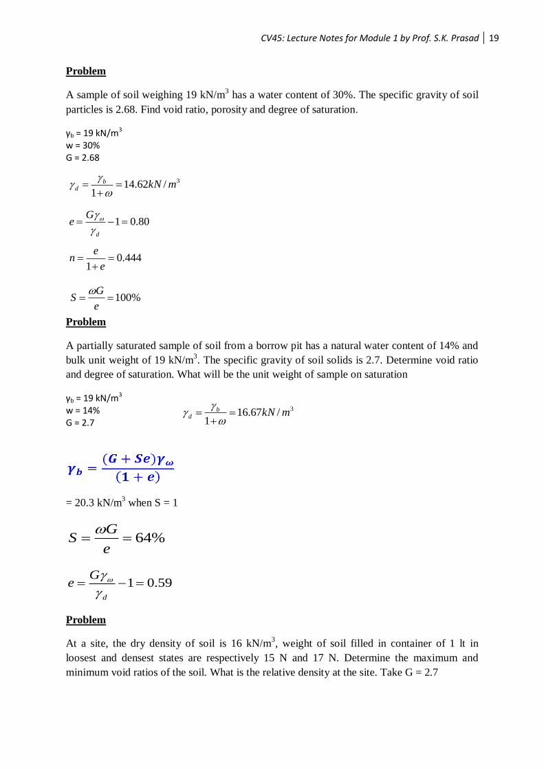
Problem
A sample of soil weighing 19 kN/m3 has a water content of 30%. The specific gravity of soil
particles is 2.68. Find void ratio, porosity and degree of saturation.
γb = 19 kN/m3 w = 30% G = 2.68
Problem
A partially saturated sample of soil from a borrow pit has a natural water content of 14% and
bulk unit weight of 19 kN/m3. The specific gravity of soil solids is 2.7. Determine void ratio
and degree of saturation. What will be the unit weight of sample on saturation
γb = 19 kN/m3 w = 14% G = 2.7
= 20.3 kN/m3 when S = 1
Problem
At a site, the dry density of soil is 16 kN/m3, weight of soil filled in container of 1 lt in
loosest and densest states are respectively 15 N and 17 N. Determine the maximum and
minimum void ratios of the soil. What is the relative density at the site. Take G = 2.7
%64e
GS
59.01d
Ge
3/62.141
mkNbd
80.01d
Ge
0.4441
e
en
%100e
GS
3/67.161
mkNbd

CV45: Lecture Notes for Module 1 by Prof. S.K. Prasad 20
1.10 Distinction between Mass Density and Weight Density
In geotechnical engineering, it is common to use weight density or unit weight than mass
density. It should be noted that weight density depends on acceleration due to gravity (g)
and hence it is place dependent. However, g does not change considerably from place to
place within the engineering limits. Commonly, symbol ρ is used to represent mass density
and symbol γ is used to represent weight density. Further, γ = ρ * g.
Table 3 : Common mass densities and Unit weights in Geotechnical Engineering
Mass Density (kg/m3)
Unit weight (kN/m3)
Bulk ρb γb
Dry ρd γd
Soil Solids ρs γs
Water ρω γω
Saturated ρsat γsat
Submerged ρsub γsub
ρω = 1000 kg/m3
γω = 9800 N/m3 = 9.8 kN/m3

CV45: Lecture Notes for Module 1 by Prof. S.K. Prasad 21
INDEX PROPERTIES OF SOIL
1.11 GENERAL
Index properties are the properties of soil that help in identification and classification of soil.
Water content, Specific gravity, Particle size distribution, In situ density (Bulk Unit weight of
soil), Consistency Limits and relative density are the index properties of soil. These
properties are generally determined in the laboratory. In situ density and relative density
require undisturbed sample extraction while other quantities can be determined from
disturbed soil sampling.
The following are the Index Properties of soil.
1. Water content
2. Specific Gravity
3. In-situ density
4. Particle size distribution
5. Consistency limits
6. Relative Density
1.12 DETERMINATION OF INDEX PROPERTIES OF SOIL
This section explains the important methods approved by Indian Standards for the
determination of Index properties of soil both in laboratory and in field.
1.12.1 Water Content
Oven drying method and Calcium carbide method are the two popular methods of
determination of water content. Refer to IS 2720 – Part 2- 1973 for more detail.
a) Oven Drying Method
It is an accurate method of determining water content of soil in the laboratory. The
procedure is as follows.
1. Collect a representative sample of soil in a steel cup carrying a lid.
2. Find the weight of cup and lid along with soil (W1)
3. Keep the cup with lid open in a thermostatically controlled oven for 24 hours at
around 105oC. Free water in the soil evaporates.
4. After cooling the cup, find the weight of cup and lid along with dry soil (W2)

CV45: Lecture Notes for Module 1 by Prof. S.K. Prasad 22
5. Find the empty weight of cup and lid (W3)
Why Steel cup with a lid ?
Lid should be covered after taking the sample to avoid movement of water, dust air etc.
Steel (Stainless steel) cup is used to avoid interaction between material of cup, water
and minerals & salts (if any) present in soil.
A sample calculation for the determination of water content in the laboratory by oven
drying method is presented in the table below.
Table 1: Determination of water content by Oven drying method
Sl No
Description Determination No.
I II III
1 Weight of cup + Wet Soil (W1) g 44.12 44.11 46.10
2 Weight of cup + Dry Soil (W2) g 41.18 41.16 43.01
3 Weight of cup (W3) g 20.12 20.08 20.00
CALCULATIONS
1 Weight of water = W1 – W3 2.94 2.95 3.09
2 Weight of solids = W2 – W3 21.06 21.08 23.01
3 Water content 13.96 13.99 13.43
Average Value 13.79 %
b) Calcium Carbide method or Rapid Moisture Meter Method
It is a rapid method of determination of water content of soil. It consists of an air tight
container with a diaphragm and a calibrated meter. About 6 g of soil is mixed with fresh
Calcium carbide. The mixture is rigorously shaken. Water in the soil reacts with Calcium
Carbide to release acetylene gas. The amount of gas produced depends on available water.

CV45: Lecture Notes for Module 1 by Prof. S.K. Prasad 23
This gas creates a pressure on sensitive diaphragm and water content is directly recorded on
the calibrated meter. The method is not very accurate, but is extremely rapid.
Fig. 6 : Typical picture of Rapid Moisture meter and its assembly
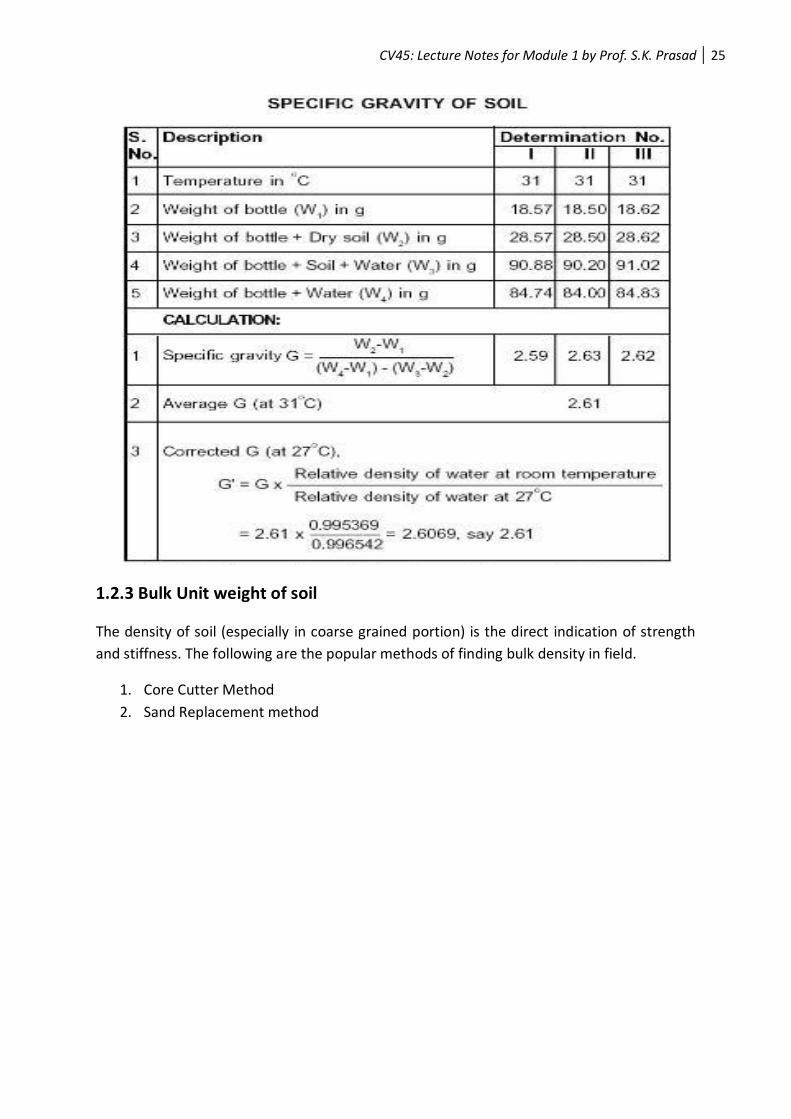
1.2.2 Specific Gravity of Soil Solids
Specific gravity of soil solids is commonly determined by Pycnometer method. Refer to IS
2720 – Part 3- Sections 1 & 2 - 1981 for more detail.
a) Pycnometer method 1. Use pycnometer for the determination of specific gravity of coarse grained fraction
and density bottle for that of fine grained fraction. 2. Find the weight of clean, dry and empty pycnometer (W1). 3. Put dry soil (about one third the height) in the pycnometer and find the weight (W2). 4. Add water till the top such that the air bubbles are completely removed and find the
weight (W3). 5. Empty the soil and fill water up to the top in the pycnometer and find the weight
(W4).
1234
12
2314
12
)()( WWWW
WW
WWWW
WW
waterofvolumeequalofWeight
SoilofWeightG
If the specific gravity is determined using any other liquid (say kerosene), other than water,
then, Kosenein GGG *ker where GK is the specific gravity of the liquid.
Further, the temperature influences specific gravity. At higher temperature viscosity of
water will be less and vice versa. Viscosity of the medium affects G. The effect of
temperature should be considered as follows.
CatWaterofGravitySpecific
CtatWaterofGravitySpecificGG
o
o
t27
27

CV45: Lecture Notes for Module 1 by Prof. S.K. Prasad 24
From Indian Standard point of view 27oC is standardized.
W1 W2 W3 W4 Fig. 7 : Stages in determination of Specific Gravity of soil using Pycnometer or Density Bottle
b) Why pycnometer for coarse grained soil and density bottle for fine grained
soil?
Coarse grained soil requires larger size container owing to the bigger particle size. Large
quantity of fine grained soil is difficult to handle especially expelling out air. Hence smaller
density bottle of 50 ml capacity is used.
c) Why pycnometer has a conical top with a opening ?
The purpose of conical top is to reduce the cross section gradually to a minimum such that
any difference in level of water in different stages should not cause serious error. Further,
the opening will allow any air present in the voids of soil to be expelled out.
CV45: Lecture Notes for Module 1 by Prof. S.K. Prasad 25
1.2.3 Bulk Unit weight of soil
The density of soil (especially in coarse grained portion) is the direct indication of strength
and stiffness. The following are the popular methods of finding bulk density in field.
1. Core Cutter Method
2. Sand Replacement method

CV45: Lecture Notes for Module 1 by Prof. S.K. Prasad 26
Fig. 8 : Apparatus for field density determination of soil using Core Cutter
a) Determination of In-situ unit weight of soil by Core Cutter Method
The following are the steps involved in determination of bulk density and hence dry density
of soil at a site.
1. Refer IS 2720 – Part 29 – 1975
2. Main apparatus include Core cutter with a sharp edge, dolly or Collar and a rammer.
3. This method is applicable for soil that sticks to the surface of cutter (Clayey soil) and
that is not very stiff (where cutter can be penetrated in to ground by ramming).
4. Sampling is done vertically by ramming downwards.
5. The inner surfaces of core cutter and dolly are greased.
6. The ground surface is leveled after removing the top soil.
7. Core cutter with collar on top and sharp edge at bottom is placed on the ground.
8. It is then driven in to the ground using the rammer till the soil collects up to the
collar.
9. It is carefully taken out by loosening from outside such that the soil inside remains in
tact.
10. Dolly is carefully removed. The soil surface in the core cutter is trimmed from both
the ends.
Let, V = Volume of the core cutter
W1 = Empty weight of core cutter
W2 = Weight of core cutter with soil
Then, Bulk unit weight of soil at the site

CV45: Lecture Notes for Module 1 by Prof. S.K. Prasad 27
A representative sample of soil from the middle of core cutter is placed for the
determination of water content.
Determination of In-situ unit weight of soil by Sand Replacement Method
Fig. 9 : Apparatus for field density determination of soil from Sand Replacement approach
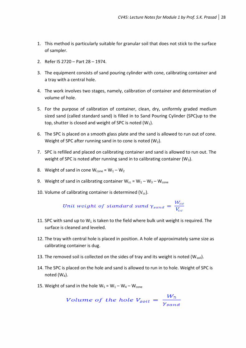
CV45: Lecture Notes for Module 1 by Prof. S.K. Prasad 28
1. This method is particularly suitable for granular soil that does not stick to the surface
of sampler.
2. Refer IS 2720 – Part 28 – 1974.
3. The equipment consists of sand pouring cylinder with cone, calibrating container and
a tray with a central hole.
4. The work involves two stages, namely, calibration of container and determination of
volume of hole.
5. For the purpose of calibration of container, clean, dry, uniformly graded medium
sized sand (called standard sand) is filled in to Sand Pouring Cylinder (SPC)up to the
top, shutter is closed and weight of SPC is noted (W1).
6. The SPC is placed on a smooth glass plate and the sand is allowed to run out of cone.
Weight of SPC after running sand in to cone is noted (W2).
7. SPC is refilled and placed on calibrating container and sand is allowed to run out. The
weight of SPC is noted after running sand in to calibrating container (W3).
8. Weight of sand in cone Wcone = W1 – W2
9. Weight of sand in calibrating container Wcc = W1 – W3 – Wcone
10. Volume of calibrating container is determined (Vcc).
11. SPC with sand up to W1 is taken to the field where bulk unit weight is required. The
surface is cleaned and leveled.
12. The tray with central hole is placed in position. A hole of approximately same size as
calibrating container is dug.
13. The removed soil is collected on the sides of tray and its weight is noted (Wsoil).
14. The SPC is placed on the hole and sand is allowed to run in to hole. Weight of SPC is
noted (W4).
15. Weight of sand in the hole W5 = W1 – W4 – Wcone

CV45: Lecture Notes for Module 1 by Prof. S.K. Prasad 29
1.2.3 Particle Size Distribution
1. Soil in nature exists in different sizes, shapes and appearance. Depending on these
attributes, the soil at a site can be packed either densely or loosely. Hence, it is
important to determine the percentage of various sized soil particles in a soil mass.
This process is called particle size distribution analysis. For this purpose, a particle
size distribution curve is plotted. Packing of soil, amount of voids present influence
the strength and stability of soil mass.
The distribution of grain size influences packing. Good distribution of all sizes reduces voids
if compacted well.
Soil Type Description Average grain size
Gravel Rounded and/or angular bulky hard rock Coarse: 80 mm to 20 mm
Fine: 20 mm to 4.75 mm
Sand Rounded and/or angular bulky hard rock Coarse: 4.75 mm to 2 mm
Medium: 2 mm to 0.425 mm
Fine: 0.425 mm to 0.075 mm
Silt Particles smaller than 0.075 mm, exhibit
little or no strength when dried
0.075 mm to 0.002 mm
Clay Particles smaller than 0.002 mm, exhibit
significant strength when dried; water
reduces strength
<0.002 mm
Importance of Particle Size Distribution
1. Used for the soil classification.
2. Used to design drainage filter.
3. Used to select fill materials of embankments, earth dams, road sub-base materials.
4. Used to estimate performance of grouting, chemical injection and dynamic
compaction.
5. Effective Size, D10, can be correlated with the hydraulic conductivity.
6. More important to coarse-grained soils
a) Particle size distribution curve
It is a graph with percentage finer (N) plotted along the vertical axis (ordinate) in normal
scale and particle diameter (D) along the horizontal axis (abscissa) in logarithmic scale. It
gives an idea about the size and gradation of soil. A soil sample is well graded if it has a good
distribution of all sized particles, otherwise, it is called poorly graded. Uniformly graded
sample is a special category of poorly graded samples in which all soil particles have the

CV45: Lecture Notes for Module 1 by Prof. S.K. Prasad 30
same size. Gap graded samples possess different proportions of same sized particles in
increasing sizes. Intermediate size particles are missing. For achieving good density, well
graded soils are most suitable.
D10, D30, D60 are the important particle sizes. D10 represents a size in mm such that 10 % of
particles are finer than this size. It is some times called effective diameter. D30 and D60
represent sizes in mm such that 30 % and 60 % of particles respectively are finer than this
size obtained on the particle size distribution curve. The following terminologies are
defined.
Fig. 10 : Particle size distribution curve
Uniformity coefficient is a measure of range of particle sizes is given by,
10
60
D
DCu
Coefficient of Curvature represents the shape of particle size distribution curve and is given
by,
6010
2
30
XDD
DC c
For well graded soil, Cc should be between 1 and 3 and Cu should be greater than 4 (if gravel)
or 6 (if sand). Even if either of the two conditions is not satisfied, the sample is poorly
graded.
Particle size distribution is obtained by sieve analysis for coarse grained fractions and
sedimentation analysis for fine grained fractions. Hydrometer analysis is a popular
sedimentation analysis.

CV45: Lecture Notes for Module 1 by Prof. S.K. Prasad 31
b) Sieve Analysis
Fig. 11 : Sieve analysis for particle gradation
Refer IS 2720 – Part 4 – 1975 for more details.
A set of IS sieves are arranged in order with one having largest aperture at the top and that
with smallest aperture at the bottom. A lid at the top and a receiver at the bottom complete
the assembly.
A known weight of representative sample of soil (say 1000 g) is placed in the top sieve.
The assembly is vibrated on a sieve shaker for at least 10 minutes.
Depending on the particle size, soil is collected in different sieves. Weight of soil in each
sieve is measured.
Table 2 gives the details of calculation. Particle size distribution curve is plotted. The soil
sample is classified as well graded or poorly graded.
Table 2 : Particle size distribution Analysis
IS sieve number
Sieve size (mm)
Weight of Soil on each sieve (g)
Cumulative weight retained
% Cumulative weight retained
% Finer
4.75 4.75
2.36 2.36
1.18 1.18
600 0.600
425 0.425
300 0.300
212 0.212
150 0.150
75 0.075
Receiver
Total

CV45: Lecture Notes for Module 1 by Prof. S.K. Prasad 32
Fig. 12 : Particle size distribution curve
c) Sedimentation Analysis
It is also called wet analysis and is applicable for fine grained soils
The analysis is based on Stoke’s law which states that the velocity at which soil particles
settle in a suspension depend on shape, size and weight of particles. Assuming spherical
particles and same density, 2Dv
)1(
18
1
18
1 22
GDDv s
Here, v = Terminal velocity of sinking soil particle
D = Diameter of soil particle
γs = Unit weight of soil solids
γw = Unit weight of water
G = Specific Gravity of Soil Solids
η = Viscosity of water
The particles are assumed to settle independent of each other and without the interference
of wall of container.

CV45: Lecture Notes for Module 1 by Prof. S.K. Prasad 33
Based on the velocity of settlement, the diameter of soil particles may be computed. For the
purpose of evaluating velocity of settlement of soil particles, hydrometer analysis is
performed.
d) Hydrometer analysis
A hydrometer is a device made of glass, consisting of a bulb with calibrated weight and stem
with calibrated readings such that when placed in pure water it floats at a level giving
reading 1.000. If it floats in a denser fluid, the readings are greater than 1 (up to 1.030).
Fig. 13 : Determination of grain size distribution from Hydrometer test
Effective depth He of hydrometer depends on volume of hydrometer (Vh), height of bulb (h),
cross sectional area of jar (A) and hydrometer reading (Rh). Height above the ease of the
stem (H) is a function of Rh. He is given by, )(
2
1
A
VhHH h
e . Hence, calibration curve for
hydrometer is prepared prior to the test as shown.

CV45: Lecture Notes for Module 1 by Prof. S.K. Prasad 34
Fig. 14 : Determination of grain size distribution from Hydrometer test
Fig. 15 : Determination of grain size distribution from Hydrometer test
e) Correction for Hydrometer reading
The recorded hydrometer reading may require the following corrections depending in the
situation.
Cm : Correction for meniscus
The solution containing soil will be opaque. Hence, it is difficult to obtain reading
corresponding to lower meniscus. Rh is taken to upper meniscus and correction is applied.
The correction is always positive.
Ct : Correction for temperature

CV45: Lecture Notes for Module 1 by Prof. S.K. Prasad 35
Hydrometer is calibrated at 27oC. If the laboratory temperature is higher, the liquid will be
less viscous and hydrometer sinks more. Rh will be less than actual needing positive
correction. Similarly, low laboratory temperature requires negative correction.
Cd : Correction for dispersing agent
A dispersing agent is added to water to disperse the soil particles and allow them to settle
individually. Dispersing agent increases the density of water and hydrometer floats higher.
Therefore the correction is always negative.
Hence, corrected hydrometer reading dtmh CCCRR
Here, Rh is the observed hydrometer reading. The three corrections are known as composite
correction (C).
dtmhh CCCRCRR
Here, dtm CCCC
From the hydrometer reading R, diameter D of soil particle and corresponding percentage
finer are computed.
Limitations of Hydrometer Analysis
Assumption Reality
Sphere particle Platy particle (clay particle) as D 0.005mm
Single particle (No interference between particles & wall)
Many particles in the suspension
Known specific gravity of particles
Terminal velocity Average results of all the minerals in the particles, including the adsorbed water films.
1.2.4 Consistency Limits
Engineering Characterization of Soils

CV45: Lecture Notes for Module 1 by Prof. S.K. Prasad 36
Consistency is the relative ease with which soil can be deformed. It is applicable to fine
grained soils whose consistency depends on water content. Relative consistency can be
expressed as very stiff, stiff, medium stiff, soft, very soft with increasing water content.
Atterberg, a Swedish agriculturist in 1911 observed four states of consistency, namely,
Liquid state, Plastic state, Semi solid state and Solid state in clayey soil with changing water
content. He set arbitrary limits for these states called consistency or Atterberg’s limits.
Fig. 16 : Consistency Limits in soil
Liquid Limit (wL), Plastic Limit (wP) and Shrinkage Limit (wS) are the atterberg limits. These
limits are most useful for engineering purpose in order ro classify the soils.
a) Liquid Limit (wL) : It is the water content corresponding to an arbitrary limit between liquid and plastic states of consistency of a soil. It is a minimum water content at which soil is still in liquid state, but possessing a small shear strength and exhibiting some resistance to flow.
b) Plastic Limit (wP) : It is the water content corresponding to an arbitrary limit between
plastic and semi-solid states of consistency of a soil. It is a minimum water content at which soil will just begin to crumble when rolled in to a thread of approximately 3 mm diameter.

CV45: Lecture Notes for Module 1 by Prof. S.K. Prasad 37
c) Shrinkage Limit (wS) : It is the water content corresponding to an arbitrary limit between semi-solid and solid states of consistency of a soil. It is the lowest water content at which soil is fully saturated. It is also the maximum water content at which any reduction in water content will not reduce the volume of the soil mass.
Figure explains the three limits. Water content is plotted along the horizontal axis and volume of soil mass is plotted on the vertical axis. It can be seen that the soil mass in dry state possesses some volume. Any addition of water will not immediately increase the volume as water occupies the void space till wS is reached. Further increase in water content will continuously increase the volume of soil mass.
Determination of Liquid Limit from Casagrande approach
Fig. 17 : Determination of Liquid Limit
The water content at which a groove cut in a soil paste will close upon 25 repeated drops of
a brass cup with a rubber base.
A required amount of soil passing through a 425µm sieve is mixed with water until a
uniform consistency is achieved.
The liquid limit device is calibrated such that the height fall is 10 mm. The soil is then taken
into the cup such that the surface is parallel to the horizontal. Then using a grooving tool,
the soil is taken out such that the grooving tool is always perpendicular to the cup at the
time of contact.
Blows are given such that handle revolves at 2 revolutions per second. The number of blows
required for the soil to fail is noted and a sample along the failure plane is taken for

CV45: Lecture Notes for Module 1 by Prof. S.K. Prasad 38
moisture content determination. Best results are obtained for blows ranging between 15 to
35.
Determination of Liquid Limit by FALL CONE Method
The fall cone test is more popular in Europe. This method attempts to eliminate the
shortcomings of Casagrande test
Fall cone test for liquid limit determination consists of a Standard cone that is brought into
contact with soil and clamped. At time zero cone is released and penetration at end of 5
seconds is recorded. Water content of soil is determined, cup emptied, and test repeated as
necessary at other water contents to produce a semi-log curve of w versus penetration.
Test Procedure for Fall Cone Test
1. Obtain the soil passing through 425 micron sieve, just as for the liquid limit test. The
difference is that it is a larger quantity and is placed in the cup.
2. The cone tip is brought into contact with the soil surface and time-initialized.
3. The cone is released for a free-fall into the soil and the penetration at the end of 5
seconds is recorded.
4. Since the water content for a penetration depth of 20 mm would be a chance
occurrence, several trials at different water contents on both sides of 20-mm
penetration are used to construct a semi-log plot of penetration versus water
content.
5. In one point test, the liquid limit is obtained as follows
where x = Penetration in mm
ω = Water content corresponding to penetration x
Table 3: Distinctions between Casagrande and Fall Cone methods
Casagrande Method Fall Cone Method
Professor Casagrande standardized the test and developed the liquid limit device.
Developed by the Transport and Road Research Laboratory, UK.
Multipoint test. Both Multipoint & One-point test.
Resistance to flow. Resistance to penetration.
At low ωL slightly lower values At low ωL slightly higher values

CV45: Lecture Notes for Module 1 by Prof. S.K. Prasad 39
Determination of Plastic Limit
The moisture content at which a thread of soil just begins to crack and crumble when
rolled to a diameter of 3 mm. The plastic limit (ωP) is the water content (w%) where soil
starts to exhibit plastic behavior. It is the water content at which a soil changes from a
plastic consistency to a semi-solid consistency. It was developed by Atterberg in 1911. The water content at which a 3 mm thread of soil can be rolled out but it begins to crack
and cannot then be re-rolled was arbitrarily defined as Plastic limit.
Fig. 18 : Determination of Plastic Limit
Determination of Shrinkage Limit
It is the water content where further loss of moisture will not result in any more volume
reduction. It is much less commonly used than the liquid limit and the plastic limit. It is the
water content at which the soil volume ceases to change.
Fig. 19 : Determination of Shrinkage Limit

CV45: Lecture Notes for Module 1 by Prof. S.K. Prasad 40
Soil volume: V, Soil weight: W Soil volume: Vd, Soil weight: Wd
Before drying After drying
Here. W = Initial weight of soil
Wd = Dry weight of soil
V = Initial volume of soil
Vd = Dry volume of soil
γω = Unit weight of water
The following are a few important definitions.
d) Plasticity : It is the property of soil that allows it to deform rapidly without rupture,
elastic rebound and volume change. The thin film of water adhering to clay particles is
responsible for its plastic behavior.
e) Plasticity Index (IP) : It is the difference between liquid and plastic limits. A soil with IP = 0
is called non-plastic (NP). Higher the IP, more plastic will be the soil.
PLPI
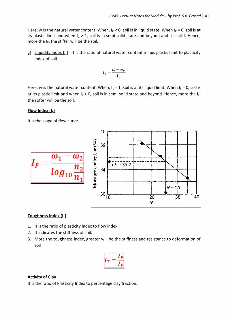
f) Consistency Index (IC) : It is the ratio of liquid limit minus natural water content to
plasticity index of soil.
P
LC
II
CV45: Lecture Notes for Module 1 by Prof. S.K. Prasad 41
Here, w is the natural water content. When, IC < 0, soil is in liquid state. When IC = 0, soil is at its plastic limit and when IC > 1, soil is in semi-solid state and beyond and it is stiff. Hence, more the IC, the stiffer will be the soil. g) Liquidity Index (IL) : It is the ratio of natural water content minus plastic limit to plasticity
index of soil.
P
PL
II
Here, w is the natural water content. When, IL = 1, soil is at its liquid limit. When IL = 0, soil is
at its plastic limit and when IL < 0, soil is in semi-solid state and beyond. Hence, more the IL,
the softer will be the soil.
Flow Index (IF)
It is the slope of flow curve.
Toughness Index (IT)
1. It is the ratio of plasticity index to flow index.
2. It indicates the stiffness of soil.
3. More the toughness index, greater will be the stiffness and resistance to deformation of
soil
Activity of Clay
It is the ratio of Plasticity Index to percentage clay fraction.

CV45: Lecture Notes for Module 1 by Prof. S.K. Prasad 42
Type of Clay Activity
Inactive Clay < 0.75
Normal Clay 0.75 – 1.25
Active Clay > 1.25
1. It was proposed by Skempton (1953).
2. Plasticity Index is influenced by both the amount and type of clay. Activity separates
this effect.
3. Higher the activity of clay, greater will be the volume increase when wetted, and
greater will be shrinkage when dried.
Determination of Density Index
Please refer to IS 2720 – Part 14 – 1983.
To find emax
1. Fill 1000 ml graduated glass cylinder up to 500 ml with distilled water.
2. Place a large funnel on top such that its bottom tip is in water.
3. Slowly place dry soil in to cylinder through the funnel such that particles settle uniformly
& independently.
4. Measure the weight and volume of soil to find dry density and hence emax
To find emin
1. Place the soil in compaction mould with collar in wet state.
2. Using needle vibrator compact it and add more soil to fill beyond collar.
3. Remove the collar and level the soil. Find the volume and dry weight and hence dry
density. emin can be determined later.
or
mmfractionclay
weightfractionclay
PIA
002.0:
)(%

CV45: Lecture Notes for Module 1 by Prof. S.K. Prasad 43
1.13 Numerical problems on Index Properties Determination
Problem 10
A sample of soil was tested for water content determination and the following were the
results. Find water content.
Weight of empty cup = 55 g
Weight of cup + wet soil = 88 g
Weight of cup + soil after oven drying = 82 g
Solution
Weight of water = 6 g
Weight of solids = 27 g
Water content = 22.2 %
Problem 11
A sample of clayey soil was collected for the determination of water content. The following
are the details of measurement. Find water content. If the soil is fully saturated find
porosity. Take G = 2.7.
Weight of empty cup = 60 g
Weight of wet soil + cup = 120 g
Weight of dry soil + cup = 100 g (after drying in oven)
Solution
Weight of water = 120 – 100 = 20 g
Weight of dry soil = 100 – 60 = 40 g
Water content = 50%
If the soil is fully saturated, e = ωG = 1.35
Porosity n = 0.574
Problem 12
A Specific Gravity test is performed on river sand and the following are the results.
Weight of pycnometer = 900 g
Weight of pycnometer + dry soil = 1300 g
Weight of pycnometer + soil + water = 3050 g
Weight of pycnometer + water = 2800 g
The test was performed at 5oC during winter. Find G
Specific Gravity of water at 5oC = 1.000
Specific Gravity of water at 27oC = 0.997
Solution

CV45: Lecture Notes for Module 1 by Prof. S.K. Prasad 44
Problem 13
The following are the results of specific gravity test on locally available sand.
Weight of pycnometer = 800 g
Weight of pycnometer + soil + water = 2800 g
Weight of pycnometer + water = 2600 g
G = 2.7
Find the weight of dry soil taken in the pycnometer in the beginning.
Problem 14
A density bottle was used to find specific gravity of clay and kerosene was the liquid
medium instead of water. Find G given the following details.
Weight of density bottle = 80 g
Weight of density bottle + dry soil = 110 g
Weight of density bottle + soil + kerosene = 141 g
Weight of density bottle + kerosene = 120 g
Specific Gravity of kerosene = 0.8

CV45: Lecture Notes for Module 1 by Prof. S.K. Prasad 45
Problem 15
A core cutter of 100 mm internal diameter and 128 mm height was used to determine
the unit weight of soil at a site. The total weight of core cutter and soil was 3015 g and
empty weight of core cutter was 1374 g. A representative sample of soil was kept in a
steel cup of weight 60 g for the determination of water content. Weights of cup and soil
before and after placing in oven were respectively 106.4 g and 92 g. Find dry unit weight
of soil and degree of saturation if G = 2.7.
Weight of core cutter + soil = 3015 g
Weight of core cutter = 1374 g
Weight of soil = 1641 g
Volume of core cutter = 0.785D2H = 1.048 X 10⁻³ m3
Bulk Unit weight of soil = 15.66 kN/m3
Weight of water = 14.4 g
Weight of solids = 32 g
Water content = 45%
Dry unit weight = 10.8 kN/m3
Void ratio e = 1.45
Degree of Saturation S = 83.8%
Problem 16
The following are the results of test for in situ bulk unit weight at a site by sand replacement
method. Find γb and ρb.
Initial weight of sand and SPC W1 = 10550 g
Weight of sand in SPC after pouring in to cone W2 = 10105 g
Weight of sand in SPC after pouring in to calibrating container W3 = 8655 g
Weight of sand in SPC after pouring in to hole W4 = 8512 g
Diameter of Calibrating container = 100 mm
Height of Calibrating container = 127.3 mm
Weight of soil Wsoil = 1820 g

CV45: Lecture Notes for Module 1 by Prof. S.K. Prasad 46
Problem 17
A sample of 1000 g of soil from a site was performed sieve analysis. The weights of soil
collected on each sieve are presented in the tabular entry. Find effective diameter, D30, D60
and coefficients of uniformity and curvature.
IS sieve
number
Sieve size
(mm)
Weight of Soil on
each sieve (g)
Cumulative
weight retained
% Cumulative
weight retained
% Finer
4.75 4.750 60 60 6 94
2.36 2.360 110 170 17 83
1.18 1.180 150 320 32 68
600 0.600 170 490 49 51
425 0.425 110 600 60 40
300 0.300 120 720 72 28
212 0.212 90 810 81 19
150 0.150 60 870 87 13
75 0.075 80 950 95 5
Receiver 50 1000 100 0
Total 1000
Fig. 1 : Particle size distribution curve

CV45: Lecture Notes for Module 1 by Prof. S.K. Prasad 47
Problem 18
A soil sample of particle size ranging from 0.075 mm to 0.003 mm is put on top of the water
surface in a tank. Depth of water in the tank is 3 m. Estimate the time required for the first
particle and also the entire sample to reach the bottom of tank. Assume μ = 0.01 poise and
G = 2.7
Note: μ = Absolute viscosity (Poise)
1 Poise = 1 N-s/m2/g = 1 N/m-s
Viscosity η = μ/g 1 N/m-s/9.8 m/s2 = 0.102 N-s/m2
Data
μ = 0.01 Poise
η = 0.00102 N-s/m2 = 1.02X10⁻⁶ kN-s/m2
G = 2.7
γω = 9.8 kN/m3
First particle to settle has diameter 0.075 mm
Velocity v = 5.104 X 10⁻³ m/s
In a tank of water depth 3 m, time taken for settling = 587.77 s
Last particle to settle has diameter 0.003 mm
Velocity v = 8.17 X 10⁻⁶ m/s
In a tank of water depth 3 m, time taken for settling = 367197 s
Problem 19
In a shrinkage limit test the following data was obtained.
Initial weight of soil = 1.928 N
Initial volume of soil = 106000 mm3
Weight of soil after drying = 1.46 N
Volume of soil after drying = 77400 mm3.
Find shrinkage limit and initial and final void ratios. Take G = 2.7.
Data
W = 1.928 N
V = 106000 mm3
Wd = 1.46 N
Vd = 77400 mm3
G = 2.7
γω = 9.8 kN/m3 = 9.8X10⁻⁶ N/mm3
ωS = 12.86 %
ω = 32.05%
)1(
18
1 2
GDv

CV45: Lecture Notes for Module 1 by Prof. S.K. Prasad 48
Since soil is saturated beyond shrinkage limit, S = 1
ωSG = Sefinal efinal = 0.35
ωG = Seinitial einitial = 0.87
Problem 20
A clayey soil was tested for liquid and plastic limits and the following were the results. Find
plasticity index, flow index, toughness index, consistency index and liquidity index. Plastic
Limit was found to be 28% and natural water content was 35%.
Number of Blows 34 23 18 12
Water Content 44.6 49.4 51.4 55.6
ω = 35%
ωP = 28%
ωL = 48.5%
IP = 20.5%
ω1 = 55.6%
ω2 = 44.6%
n1 = 12
n2 = 34
IF = 24.3%
IT = 0.84
IL = 0.34
IC = 0.66

CV45: Lecture Notes for Module 1 by Prof. S.K. Prasad 49
SOIL CLASSIFICATION
1.14 Introduction
Soil classification is the arrangement of soils into different groups such that the soils
in a particular group have similar behavior. As there are a wide variety of soils
covering earth, it is desirable to classify the soils into broad groups of similar
behavior. Soils, in general, may be classified as cohesionless and cohesive or as
coarse-grained and fine-grained. These terms, however, are too general and include
a wide range of engineering properties. Hence, additional means of classification is
necessary to make the terms more meaningful in engineering practice.
1.15 The need for Soil Classification
Natural soil deposits are never homogeneous in character; wide variations in
properties and behavior are commonly observed. Deposits that exhibit similar
average properties, in general, may be grouped together, as a class. Through
classification of soils one can obtain an appropriate, but fairly accurate, idea of the
average properties of the soil group or a soil type, which is of great convenience in
any routine type of soil engineering project. From engineering point of view,
classification may be made based on the suitability of a soil for use as a foundation
material or as a construction material. For complete knowledge of behavior of soils,
all the engineering properties are determined after conducting a large number of
tests. However, an approximate assessment of the engineering properties can be
obtained from the index properties after conducting classification tests. A soil is
classified according to index properties, such as particle size and plasticity
characteristics. A classification system thus provides a common language between
engineers dealing with soils. It is useful in exchanging of information and experience
between the geotechnical engineers. It is important to note that soil classification is
no substitute for exact analysis based on engineering properties. For final design of
large structures, the engineering properties should be determined by conducting
elaborate tests on undisturbed samples.

CV45: Lecture Notes for Module 1 by Prof. S.K. Prasad 50
1.16 Requirements for a Soil Classification System:
For a soil classification system to be useful to the geotechnical engineers, it should
have the following basic requirements.
1. It should have a limited number of groups
2. It should be based on the engineering properties, which are most relevant for
the purpose for which the classification has been made.
3. It should be simple and should use the terms, which are easily understood.
Any soil classification must provide with information about the probable engineering
behavior of a soil. Most of the classification systems developed satisfy the above
requirements.
1.17 Soil Classification Systems
Several classification systems were evolved by different organizations having a
specific purpose as the object. A. Casagrande (1948) describes the systems
developed and used in highway engineering, airfield construction etc. The two
classification systems, which are adopted by the US engineering agencies and the
State Departments, are the Unified Soil Classification (UCCS) and the American
Association of State Highway and Transportation Officials (AASHTO) system. Other
countries, including India, have mostly the USCS with minor modifications.
For general engineering purposes, soils may be classified by the following systems
1. Particle size classification
2. Textural classification
3. Highway Research Board (HRB) classification
4. Unified Soil Classification
5. Indian Soil Classification
1.18 Indian Standard Classification
As per I.S. Classification (IS: 1498-1970) the soil is divided into six groups:
(a) Boulders, particle size greater than 300 mm
(b) Cobble, particle size between 80 mm to 300 mm
(c) Gravel, particle size between 4.75 mm to 80 mm
(d) Sand, particle size between 0.075 mm to 4.75 mm

CV45: Lecture Notes for Module 1 by Prof. S.K. Prasad 51
(e) Silt (size), particle size between 0.002 mm to 0.075 mm
(f) Clay (size), particle size smaller than 0.002 mm (2 m)
1.19 Indian Standard Soil Classification System:
Indian Standard Soil Classification system is in many respects similar to the Unified
system. However, there is one basic difference in the classification of fine-grained
soils. The fine-grained soils in this system are sub-dived into three categories of low,
medium and high compressibility instead of two categories of low and high
compressibility in Unified soil classification system.
Soils are divided into three broad divisions:
1) Coarse-grained soils, when 50 % or more of the total material by weight retained
on 75 m IS sieve.
2) Fine-grained soils, when more than 50 % of the total material passes 75 m IS
sieve.
3) If the soil is highly organic and contains a large percentage of organic matter and
particles of decomposed vegetation, it is kept in a separate category marked as peat
(Pt)
In all, there are 18 groups of soils
Coarse-grained soils – 8 groups
Fine-grained soils – 9 groups
Peat - 1 group

CV45: Lecture Notes for Module 1 by Prof. S.K. Prasad 52
Coarse-Grained Soils
The classification of coarse-grained soils is done on the basis of their grain and
gradation characteristics as illustrated in Table, when the fines (75 m) present in
them are less than 5 % by weight. Coarse-grained soils are sub-dived into gravel
and sand. The soil is termed gravel (G) when more than 50 % of coarse fraction (>75
m) is retained on 4.75 mm IS sieve, and termed sand (S) if more than 50 % of
coarse fraction is smaller than 4.75 mm IS sieve. These are further sub-divided as
given in Table into 8 groups.
Coarse-grained soils which contain more than 12 % fines (< 75 m) are classified as
GM or SM if fines are silty in character (meaning, the limits plot below the A-line on
the plasticity chart). On the other hand they are classified as GC or SC if the fines
are clayey in character (meaning the limits plot above the A-line on the plasticity
chart).
Fine-grained Soils
The fine-grained soils are classified on the basis of their plasticity characteristics
using the I.S Plasticity chart shown in Fig. The fine-grained soils are further divided
into three sub-divisions depending upon the values of the liquid limit:
a) Silts and clays of low compressibility – These soils have a liquid limit less than 35
% (represented by a symbol L)
b) Silts and clays of medium compressibility – These soils have a liquid limit > 35 %
but < 50 % ( represented by a symbol I)
c) Silts and clays of high compressibility – These soils have a liquid limit > 35 %
(represented by a symbol H)
Fine-grained soils are further sub-divided, as given in table in 9 groups.
Boundary Classifications:
Sometimes, it is not possible to classify to classify a soil into any one of 18 groups
discussed above. A soil may possess characteristics of two groups, either in particle
distribution or in plasticity. For such cases, boundary classifications occur and dual
symbols are used.
CV45: Lecture Notes for Module 1 by Prof. S.K. Prasad 53
a) Boundary classification for coarse-grained soils:
Coarse-grained soils having 5 % to 12 % fines are borderline cases and given a dual
symbol. While giving dual symbols, first assume a coarse soil and then a finer soil
i.e., the first part of the symbol is indicative of the gradation of coarse fraction, while
the second part indicates the nature of fines.
For example, a soil with the dual symbol SW-SC is a well-graded sand with ‘clayey’
fines that plot above A-line.
(i) Boundary classifications within gravel or sand groups can occur. The following
classification are common
GW-GP, GM-GC, GW-GM, GW-GC, GP-GM,
SW-SP, SM-SC, SW-SM, SW-SC, SP-SM.
(ii) Boundary classifications can occur between the gravel and sand groups such as
GW-SW, GP-SP, GM-SM, and GC-SC
Note: The rule for correct classification is to favour the non-plastic classification.
For eg. A gravel with 10 % fines, Cu = 20 and Cc = 2 and IP= 6 will be classified as
GW – GM, and not GW – GC.
b) Boundary classification for fine-grained soils:
Fine-grained soils also can have dual symbols.
(i) If the limits plot in the hatched zone on the plasticity chart, i.e., IP between 4 and
7, the soil has a group symbol CL – ML.
(ii) If the position of the soil on the plasticity chart falls close to the A-line, dual
symbol is used, such as CI – MI , CH – MH
(iii) If the liquid limit is very close to 35 % or 50 %, dual symbols are used, such as
ML – MI, MI – MH, CL – CI, CI – CH, OL – OI, OI – OH.
c) Boundary classification between coarse-grained and fine-grained soils:
Dual symbols can also be used when the soils have about equal percentage of
coarse – grained and fine – grained fractions. The possible dual symbols in this case
are GM – ML, GM – MI, GM – MH, GC – CL, GC – CI, GC – CH, SM – ML, SM – MI,
SM – MH, SC – CL, SC – CI, SC – CH.

CV45: Lecture Notes for Module 1 by Prof. S.K. Prasad 54
Step-by-step procedure:
A step-by-step procedure for classifying the soils as per IS: 1498 –1970 is illustrated
below:
1. Determine whether the given soil is of organic origin or coarse-grained or fine
grained.
An organic soil is identified by its colour (brownish black or dark) and characteristic
odour. If 50 % or more of the soil by weight is retained on the 75 m sieve, it is
coarse-grained, if not, it is fine-grained.
2. If the soil is coarse-grained:
(a) Obtain the GSD curve from a sieve-analysis. If 50 % or more of the coarse
fraction (>75 m) is retained on the 4.75 mm sieve, classify the soil as gravel (G); if
not, classify it as sand (S)
(b) If the soil fraction passing through the 75 m sieve is less than 5 %, determine
the gradation of the soil by calculating Cu and Cc from the GSD curve. If well graded
(according to the criteria laid down), classify the soil as GW or SW; if poorly graded,
classify as GP or SP.
(c) If more than 12 % passes through the 75 m sieve, perform the liquid limit and
plastic limit tests on the soil fraction passing though the 0.425-mm sieve. Use the I.S.
plasticity chart to determine the classification (GM, SM, GC, SC, GM–GC or SM–SC)
(d) If between 5 % and 12 % passes through the 75 m sieve, the soil is assigned a
dual symbol appropriate to its gradation and plasticity characteristics. (GW–GM,
GW–GC, GP–GC, GP–GM, SW-SM, SW-SC, SP–SC, SP-SM)
3. If the soil is fine-grained (inorganic):
(a) Determine wL and wP on the minus 0.425 mm sieve fraction and determine the
plasticity index.
(b) If the limits plot below the A – line, classify as silt (M). Further, if wL is less than
35, classify as ML; if wL is between 35 – 50 %, classify as MI; if wL is greater than 50, classify as
MH.
(c) If the limits plot above the A – line, classify as clay ©. Assign the group symbol
CL or CI or CH, depending on the value of liquid limit, as in (b).
(d) If the limits plot in the hatched zone, classify as CL – ML. If the limits plot close to
the A – line or close to wL= 35 % or wL= 50 % lines, assign dual symbols as outlined
earlier.

CV45: Lecture Notes for Module 1 by Prof. S.K. Prasad 55
4. If the soil is of organic origin, the plasticity chart is used after determining wL and
wP and the soil classified as OL, OI or OH.
5. If the soil has about 50 % each of fines and coarse – grained fractions,
(a) Determine whether the coarse – grained fraction is gravel (G) or sand (S)
(b) Determine wL and wP on the minus 0.425 mm fraction
(c) Depending on whether the limits plot above the A – line or below the A – line,
classify as C or M
(d) Based on wL, classify as L, I or H
(e) Assign the dual symbol from the information obtained in steps (a), (b), (c), and (d)
as for example, GM – ML, GM – MI, etc.,
Fig. Plasticity Chart as per IS 1498 - 1970

CV45: Lecture Notes for Module 1 by Prof. S.K. Prasad 56
Major Divisions Group
Symbol Typical Names Field Identification
procedures Information
required for
describing soils
CO
AR
SE
-GR
AIN
ED
SO
ILS
More
than
hal
f of
mat
eria
l is
lar
ger
75 μ
m s
ieve
size
.
The
75 μ
m s
ieve
size
is
about
the
size
par
ticl
e vis
ible
to t
he
nak
ed e
ye
GR
AV
EL
S
More
than
hal
f of
coar
se f
ract
ion i
s sm
alle
r th
an
4.7
5 m
m s
ieve
size
Cle
an g
ravel
s (l
ittl
e or
no f
ines
)
GW Well graded gravel, gravel-sand mixtures, little or no fines
Wide range in grain size and substantial amounts of all intermediate particle sizes
For undisturbed soils and information on stratification, degree of compactness, cementation, moisture conditions and drainage characteristics. Give typical name;
indicate approximate percentages of sand, gravel, maximum size, angularity, surface condition and hardness of the coarse grains, local or geologic names and
other pertinent descriptive information and symbol in parenthesis. Example: Silty and gravelly, about 20 % hard angular gravels 10
mm maximum size, rounded and sub-circular sand grains about 15 %. Non-plastic fines with low dry strength, well compacted and moist in place alluvial sand,
(SM)
GP Poorly graded gravels or gravel-sand
mixtures, little or no fines
Predominantly one size or a range of sizes with
some intermediate sizes missing
Gra
vel
wit
h f
ines
(Appre
ciab
le a
mount
of
fines
)
GM Silty gravels, poorly graded gravel-sand-silt mixtures
Non-plastic fines or fines with low plasticity (for identification procedures see ML and
MI below)
GC Clayey gravels, poorly graded gravel-sand-silt mixtures
Plastic fines (for identification procedures see CL and CI below)
SA
ND
S
More
than
hal
f of
coar
se f
ract
ion i
s sm
alle
r th
an
4.7
5 m
m s
ieve
size
Cle
an s
ands
(Lit
tle
or
no
fines
)
SW Well graded sands, gravelly sands, little or no fines
Wide range in grain size and substantial amounts of all intermediate
particle sizes
SP Poorly graded sands or
gravelly sands, little or no fines
Predominantly one size
of a range of sizes with some intermediate sizes missing
San
d w
ith f
ines
(Appre
ciab
le a
mount
of
fines
)
SM Silty sands, poorly graded sand silt
mixtures
Non-plastic fines or fines with low plasticity
(for identification procedures see ML and MI below)
SC Clayey sands, poorly graded sand-clay mixtures
Plastic fines (for identification procedures see CL and CI below)
Symbols Laboratory Classification Criteria
GW Cu Greater than 4 Cc Between 1 and 3
Determine percentage of gravel and sand from grain size curve depending on percentage of fines (fraction smaller than 75 μm sieve size); coarse-grained soils are classified as follows: Less than 5 %: GW, GP, SW,SP More than 12 %: GM, GC, SM,SC 5 % to 12 % : Border line cases requiring use of dual symbols Uniformity coefficient, Coefficient of Curvature,
GP Not meeting all gradation requirements for GW
GM Atterberg limits below “A” line or Ip less than 4
Limits plotting above “A” line with Ip between 4 and 7 are border line cases requiring use of dual symbols
GC Atterberg limits above “A” line with Ip greater than 7
SW Cu Greater than 6 Cc Between 1 and 3
SP Not meeting all gradation requirements for SW
SM Atterberg limits below “A” line or Ip less than 4
Limits plotting above “A” line with Ip between 4 and 7 are border line cases requiring use of dual symbols
SC Atterberg limits above “A” line with Ip greater than 7

CV45: Lecture Notes for Module 1 by Prof. S.K. Prasad 57
Major Divisions Group
Symbol
Typical Names Identification procedures (on
fraction smaller than 425 μm sieve
size)
Information
required for
describing soils
Dry
strength
Dilatancy Toughness For undisturbed soils, add information on
structure, stratification, consistency in undisturbed and remoulded states, moisture and drainage conditions Give typical names,
indicate degree and character of plasticity, amount and maximum size of coarse grains, colour in wet condition, odour, if any, local or geologic name and
other pertinent descriptive information, and symbol in parenthesis. Example: Clayey silt, brown, slightly plastic, small percentage of fine-
sand, numerous vertical root holes, firm and fry in place; losses, (ML)
FIN
E-G
RA
INE
D S
OIL
S
More
than
hal
f of
mat
eria
l is
sm
alle
r th
an 7
5 μ
m s
ieve
size
.
The
75 μ
m s
ieve
size
is
about
the
size
par
ticl
e vis
ible
to t
he
nak
ed e
ye
SIL
TS
& C
LA
YS
of
low
com
pre
ssib
ilit
y;
liquid
lim
it
< 3
5 %
ML Inorganic silts and very fine sands, rock flour, silty or
clayey fine sand or clayey silts with none to low plasticity
None to low
Quick None
CL Inorganic clays, gravelly clays, sandy clays, lean clays of low plasticity
Medium None to very slow
Medium
OL Organic silts of low plasticity
Low Slow Low
SIL
TS
& C
LA
YS
of
med
ium
com
pre
ssib
ilit
y:
Liq
uid
lim
it
35 a
nd 5
0 %
MI Inorganic silts, silty or clayey fine-sand or clayey
silts of medium plasticity
Low Quick to slow
None
CI Inorganic clays, gravelly clays, sandy clays, silty
clays, lean clays of medium plasticity
Medium to high
None Medium
OI Organic silts and organic silty clays of medium plasticity
Low to medium
Slow Low
SIL
TS
&C
LA
YS
of
hig
h
com
pre
ssib
ilit
y
Liq
uid
lim
it
> 5
0 %
MH Inorganic silts of high compressibility, micaceous or diatomaceous fine sandy or silty soils, elastic silts
Low to medium
Slow to none
Low to medium
CH Inorganic clays of high plasticity, fat clays
High to very high
None High
OH Organic clays of medium to high plasticity
Medium to high
Slow to very slow
Low to medium
High organic soil Pt Peat and other highly organic soils with very high compressibility
Readily identified by colour, odour, spongy feel and frequently by fibrous texture
1.20 Unified Soil Classification System
Originally developed by Casagrande (1940), the Unified Soil Classification System was
used for construction during World War II. It was modified in 1952 by Bureau of
Reclamation & Corps of Engineers (USA) for the construction of geotechnical structures.
It was later adopted by ASTM & BIS (1970).
• Two broad divisions – Coarse grained and Fine grained. • Coarse grained – 8 groups
(GW, GP, GM, GC, SW, SP, SM & SC) • Fine grained – 7 groups
(ML, MH, CL, CH, OL, OH & Pt) • A Line – same eqn : Ip = 0.73 (wL-20%) • However medium plasticity range is not available here.

CV45: Lecture Notes for Module 1 by Prof. S.K. Prasad 58
1.21 Numerical problems on Soil Classification
Problem 21
Classify the following three soils as per IS S N % G % S % F Cu Cc wL wP
1 1 98 2 6.5 1.8 - -
2 1 9 90 - - 60 20
3 0 86 14 - - - -
Cu > 6, 1 < Cc < 3 1. SW 2. IP = wL – wP = 40
IP,th = 0.73(wL-20) = 29.2 < 40, Point above A Line, Clay wL > 60, Soil of High Plasticity CH 3. S Problem 22 The following results were obtained from soil test in lab. % of soil passing 0.075 mm IS sieve = 25% % of soil passing 4.75 mm IS sieve = 75% Liquid Limit = 60% Plastic Limit = 25% Uniformity Coefficient = 8 Coefficient of Curvature = 1.5 Classify the soil according to IS %G = 25%, %S = 50%, %F = 25% - Coarse Grained & Sand IP,th = 0.73(wL-20%) = 29.2% < IP, Above A Line SW-SC Problem 23 Classify the following soils as per IS
S N %G %F Cu
Cc
wL
wP
A 20 60 - - 50 35
B 60 30 - - 52 38
C 40 2 5 1.2 - -
A: MH B: GM C: S Problem 24 The following data refers to a sample of soil. % passing 4.75 mm IS sieve = 64% % passing 0.075 mm IS sieve = 6% Uniformity Coefficient = 7.5, Coefficient of curvature = 2.7 Plasticity Index = 2.5 Ans: SW-SM