Customer Equilibrium in a Single-Server System

with Virtual and System Queues

Roei Engel and Refael Hassin�

Department of Statistics and Operations Research

Tel Aviv University

June 25, 2017

Abstract

Consider a non-preemptive M/M/1 system with two first-comefirst-served queues, virtual (VQ) and system (SQ). An arriving cus-tomer who finds the server busy decides which queue to join. Cus-tomers in the SQ have non-preemptive priority over those in the VQ,but waiting in the SQ is more costly. We study two information modelsof the system. In the unobservable model customers are notified onlywhether the server is busy, and in the observable model they are alsoinformed about the number of customers currently waiting in the SQ.We characterize the Nash equilibrium of joining strategies in the twomodels and demonstrate a surprising similarity of the solutions.

Keywords: Virtual queues, equilibrium behavior in a queue-

ing system, observable queues

1 Introduction

Virtual queueing is an innovative method which is now commonly usedto improve customer service satisfaction. Virtual queues, and theiruse in real life applications are extensively discussed in the literature.Examples include hospitality organizations, restaurants, amusementparks, airports, and call centers; see Armony and Maglaras [4, 5], Bur-gain, Feron, and Clarke [6], Camulli [7], Cope, Cope and Davis [10],Dickson, Ford, and Laval [11], Lovejoy, Aravkin, and Schneider-Mizell[25], de Lange, Samoilovich, and van der Rhee [24]. These systemsoffer an arriving customer the option of receiving a call when his time

�This research was supported by the Israel Science Foundation (grants No. 1015/11

and 355/15)

1

for service arrives, thereby reducing waiting costs by freeing him toperhaps perform useful activities while waiting.

Understanding the impact a virtual queue has on customer behav-ior and customer satisfaction is a central managerial issue for servicesystems of this type. However, modeling and analyzing such systemsis not simple because it involves customers’ strategic decisions. More-over, a customer’s decision and welfare strongly depend on the strate-gies adopted by the other customers of the system, and for this reasonwe look for equilibrium behavior.

Some virtual queueing systems maintain the first-come first-servedorder (calling back the customer when his turn arrives), whereas othervirtual queueing systems give priority to customers who choose to waitin the system queue and call back virtual queue customers when theserver become idle. Our model considers a system of the latter type.

We model a service system with two first-come first-served queues,a system queue (SQ) and a virtual queue (VQ) with a different wait-ing cost per unit of time. An arriving customer who finds the serveridle enters service immediately, but if the server is busy the customerchooses which queue to join, based on the waiting costs and the avail-able information. Our goal is to determine the (Nash) equilibrium ofthe system in two information models: an unobservable model wherethe customer is only informed whether the server is busy, and an ob-servable model where customers are also informed on the length of theSQ and they follow a threshold strategy, joining the SQ if its length isbelow a critical value, and possibly randomizing at that value.

Let Cs and Cv denote the waiting cost per time unit in the SQ andVQ, respectively. The system is defined by two normalized parameters,the cost ratio ϕ = Cv/Cs, and the system utilization ρ. Our mainresults are the following:

� The unobservable model. We characterize the equilibriumsolutions. Joining the SQ is a dominant strategy if ϕ > 1 − ρ,joining the VQ is dominant if ϕ < 1− ρ, and any pure or mixedjoining strategy is an equilibrium when ϕ = 1− ρ.

� The observable model. We derive formulas for the stationaryprobabilities, the mean busy period in the SQ, the expected num-ber of customers and expected waiting time in the VQ. We derivea linear-time algorithm for the truncated steady-state distribu-tion and conduct a numerical investigation of the best responseand equilibrium customers strategy. We conclude that, similarto the unobservable case, if ϕ is significantly greater than 1− ρ,joining the SQ is a dominant strategy; if it is significantly smaller,joining the VQ is dominant. In other cases, where ϕ and 1−ρ areapproximately of the same size, we obtain the “follow-the-crowd”(FTC) behavior which is typical in priority systems, and leads to

2

multiple equilibria [17, 18].

The stationary distribution in the observable case with a purethreshold strategy and preemption is investigated by Haviv [19]

�12.2.4

as a special case of a model analyzed by Kopzon, Nazarathy and Weiss[22]. In our generalized analysis of these results customers apply amixed threshold strategy and we compute the resulting customer equi-librium.

Customer decision-making and Nash equilibrium in queues were ini-tially defined and investigated by Naor [27], Littlechild [28] and Edelsonand Hildebrand [13]. The literature on strategic behavior in queueingsystems is surveyed in [18, 16].

Our paper is the first to consider customer strategic behavior andthe resulting equilibrium in a virtual queueing system where waitingcosts in the VQ are lower but the SQ obtains priority. We now describethe most relevant literature and emphasize where these papers differfrom ours.

Guijarro, Pla, and Tuffin [14] (in their second model) investigate anunobservable multi-server system with an SQ and a VQ with differentadmission costs. The queues are managed by competing servers andeach profits from its own queue. The authors investigate a two-stagesequential game where the servers choose admission prices and thecustomer chooses the queue to join. Hassin [15] and Altman, Jimenez,Nunez-Queija, and Yechiali [3] consider a system with two servers eachwith a different queue and identical waiting costs. An arriving cus-tomer can only see the length of one queue and decides which queue tojoin based on the conditional expected length of the other queue. Man-delbaum and Yechiali [26], investigate the optimal strategy of a singlearriving “smart” customer in a single server system. The customer canjoin the queue, leave the system, or delay his decision and wait outsideof the queue at a reduced cost, which can be viewed as joining a pri-vate virtual queue. Economou and Kanta [12] consider a single-serversystem with no waiting space (no SQ), where customers who find theserver busy automatically join the VQ. After completing service theserver seeks a customer in the VQ, with an exponentially distributedsearch time. If a new customer arrives during the search time the serverinterrupts the search and serves the new customer. The authors solvethe social-optimization and profit-maximization problems of both theobservable and the unobservable cases. This model with immediatesearch time can be considered as a special case of our model whereonly the VQ exists.

Some other papers analyze virtual queueing systems but customerbehavior is not a result of strategic self-optimization and thereforeno equilibrium behavior is considered. Aguir, Karaesmen, Aksin, andChauvet [2] investigate a multi-server call center system with an SQ

3

and a VQ where customers are impatient and can balk or jockey fromthe SQ to the VQ. Chakravarthy, Krishnamoorthy and Joshua [8]model a multi-server system where new arrivals who find all serversbusy join a VQ and retry after exponentially distributed time inter-vals. Moreover, upon service completion, with a given probability pthe server serves a customer from the VQ if one exists. Our model,in contrast, assumes a single server, no retrials, p = 1, and customerschoosing between the VQ and an SQ. Iravani and Balcioglu [21] con-sider a multi-server system with an SQ and a VQ where impatient cus-tomers choose a queue with an exogenous probability. Wuchner, Sztrikand de Meer [29] numerically analyze a system with an SQ and a VQwhere customers are allowed to balk and move between the queues.Kostami, and Ward [23] model a single server with inline (system) andoffline (virtual) queues where arriving customers choose which queueto join according to waiting time estimates by the server, and offlinecustomers may leave the system without informing the server. Armonyand Maglaras [4, 5] investigate two close models of a multi-server callcenter system with an SQ and a VQ, customers choose a queue to joinor balk, and those joining the VQ are guaranteed an upper bound ontheir delay. There is no waiting-cost difference between the queues,and after each service the server decides whether to take a caller fromthe SQ or from the VQ.

Our system is priority-based, and customers in the SQ have priorityover those who join the VQ. However, the main difference between oursystem and the common two-priority system is in our assumption thatthere is a different waiting cost for each queue and only the SQ isobservable. The fundamental model involving customer decisions inqueues with priorities is analyzed by Adiri and Yechiali [1] and byHassin and Haviv [17]. Both queues are observable, and the waitingcost in both is identical but the admission price is different. Hassinand Haviv [18],

�4.2 solve the unobservable case of that system.

This paper is structured as follows. Section 2 presents the basicmodel and assumptions. In section 3 we solve the unobservable model.Section 4 investigates the observable model when the customers usemixed strategies. Section 5 suggests directions for future work. Anappendix with a table summarizing our notation and detailed deriva-tions of the stationary probabilities in the observable case concludesthe paper.

2 The system

We consider a non-preemptive single-server M/M/1 system with twoqueues, a System Queue (SQ) and a Virtual Queue (VQ) which is oftencalled in the literature an orbit queue or a standby queue. An arriving

4

customer who finds the server idle enters service immediately. If theserver is busy, the customer decides whether to join the VQ or the SQ(no balking allowed). Each queue has a different waiting cost per unittime, Cs for the SQ and Cv for the VQ (Cv < Cs). The discipline ineach queue is FCFS, customers arrive according to a Poisson processat rate λ, and service times are exponentially distributed with rate µ.The system parameters λ, µ, Cs and Cv are known to the customers.(We will see that it is sufficient that they know the ratios λ/µ andCv/Cs.) If the SQ is not empty, the first customer in it will be thenext to be served when the current service terminates. Only if the SQis empty the server calls the first customer from the VQ. We considertwo information cases, an unobservable queue in which an arrivingcustomer is only informed of the state of the server - busy or idle, andan observable queue where the arriving customer is also informed ofthe number of customers currently waiting in the SQ.

3 The unobservable model

In the unobservable model arriving customers are only informed if theserver is busy or not. An arriving customer who finds the server busywill use, in general, a mixed strategy and join the SQ with some prob-ability rs. The arrival rates to the SQ and VQ when the server is busyare λrs and λ(1− rs), respectively. We define the following normalizedparameters:

ϕ =Cv

Cs

, ρ =λ

µ, ρs =

λrsµ

, ρv =λ(1− rs)

µ.

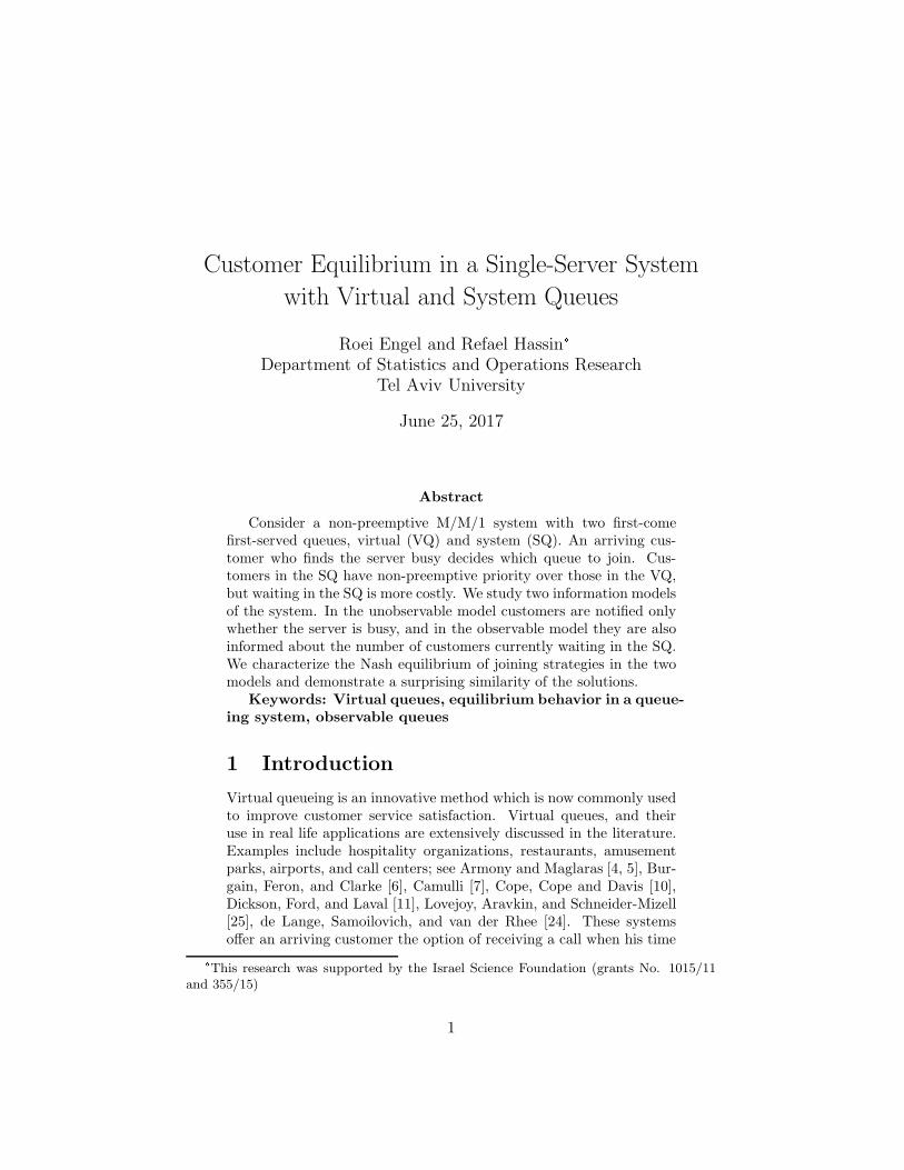
For stability we assume ρ < 1.We denote the state of the system as (ls, lv) where ls and lv are the

number of customers in SQ and the VQ, respectively. We representthe state when the server is idle with the special tag 0′. The transitionrate diagram of the system is shown in Figure 1.

Theorem 3.1.

res =

1 ϕ > 1− ρ ,

0 ϕ < 1− ρ .

If ϕ = 1− ρ, any strategy 0 ≤ res ≤ 1 defines an equilibrium.

Proof. Let B denote the event that the server is busy. Let Ws and Wv

denote the queueing time in the SQ and VQ, respectively. Given thatthe server is busy, the SQ is an M/M/1 system with arrival rate λrs,and therefore the expected time in the system of a joining customer is

E(Ws|B) =1

(1− ρs)µ. (1)

5

0′ 0, 0 1, 0 2, 0 3, 0

0, 1 1, 1 2, 1 3, 1

0, 2 1, 2 2, 2 3, 2

0, 3 1, 3 2, 3 3, 3

. . .

. . .

. . .

. . .

. . . . . . . . . . . . . . .

ls

lv

λ λrs λrs λrs

λrs λrs λrs

λrs λrs λrs

λrs λrs λrs

λrs

λrs

λrs

λrs

λrv λrv λrv λrv

λrv λrv λrv λrv

λrv λrv λrv λrv

λrv λrv λrv λrv

µ µ µ µ

µ µ µ

µ µ µ

µ µ µ

µ

µ

µ

µ

Figure 1: Transition rate diagram for the unobservable model

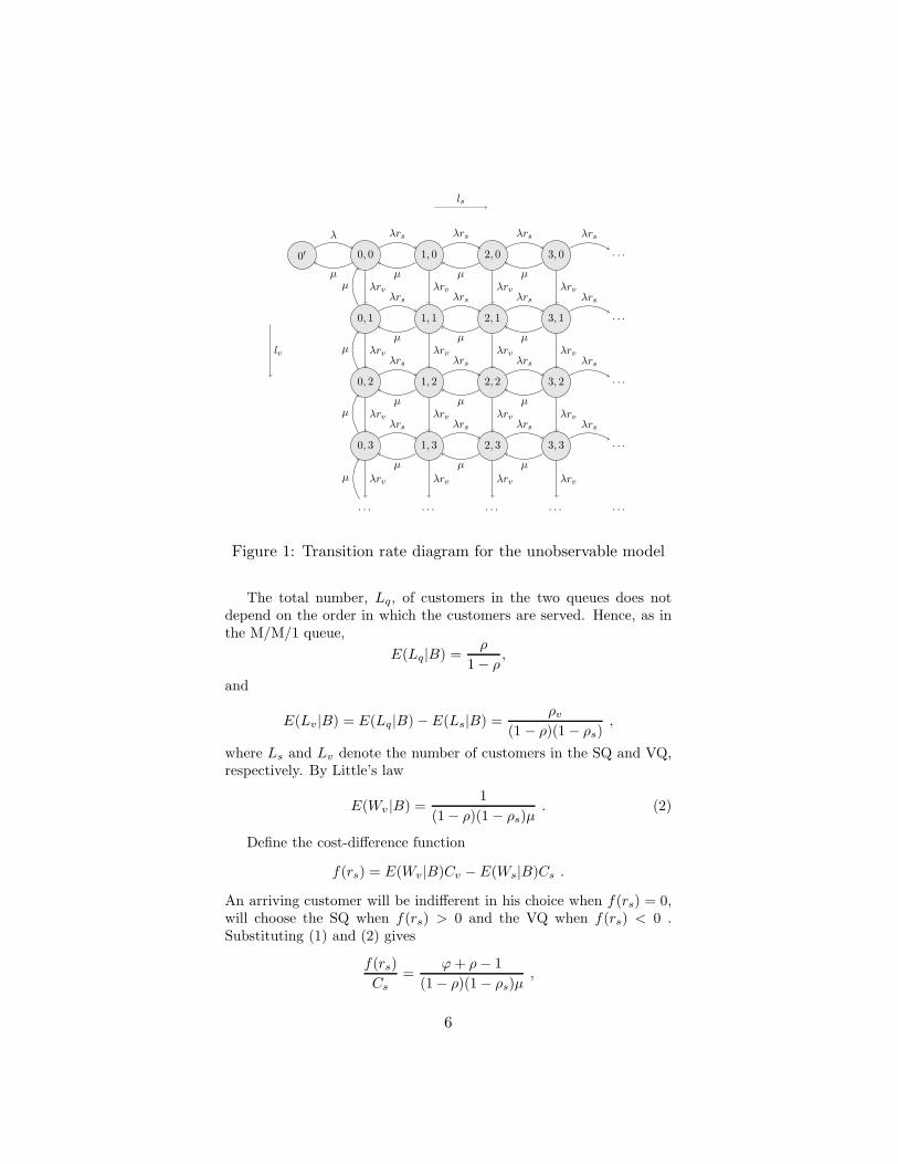
The total number, Lq, of customers in the two queues does notdepend on the order in which the customers are served. Hence, as inthe M/M/1 queue,

E(Lq|B) =ρ

1− ρ,

and

E(Lv|B) = E(Lq|B)− E(Ls|B) =ρv

(1 − ρ)(1− ρs),

where Ls and Lv denote the number of customers in the SQ and VQ,respectively. By Little’s law

E(Wv |B) =1

(1− ρ)(1 − ρs)µ. (2)

Define the cost-difference function

f(rs) = E(Wv|B)Cv − E(Ws|B)Cs .

An arriving customer will be indifferent in his choice when f(rs) = 0,will choose the SQ when f(rs) > 0 and the VQ when f(rs) < 0 .Substituting (1) and (2) gives

f(rs)

Cs

=ϕ+ ρ− 1

(1− ρ)(1 − ρs)µ,

6

from which the claim follows.

4 The observable model

In the observable case, an arriving customer is informed about thestate of the server and the number of customers, ls, in the SQ. Weassume that customers follow a threshold strategy defined as follows(see [15]):

A threshold strategy s(ls) to join the SQ with threshold T = n+ r(n ∈ N, r ∈ [0,1)) is defined by

s(ls) =

1 ls < n

r ls = n

0 ls > n .

By following this strategy a customer always joins the SQ when ls isat most n − 1, joins the VQ if it is greater than n, and joins the SQwith probability r when ls = n. When r > 0, the number of customersin the SQ is at most n+1. When r = 0, s(ls) is a pure strategy and acustomer who observes a queue of length n joins the VQ.

4.1 Steady-state solution

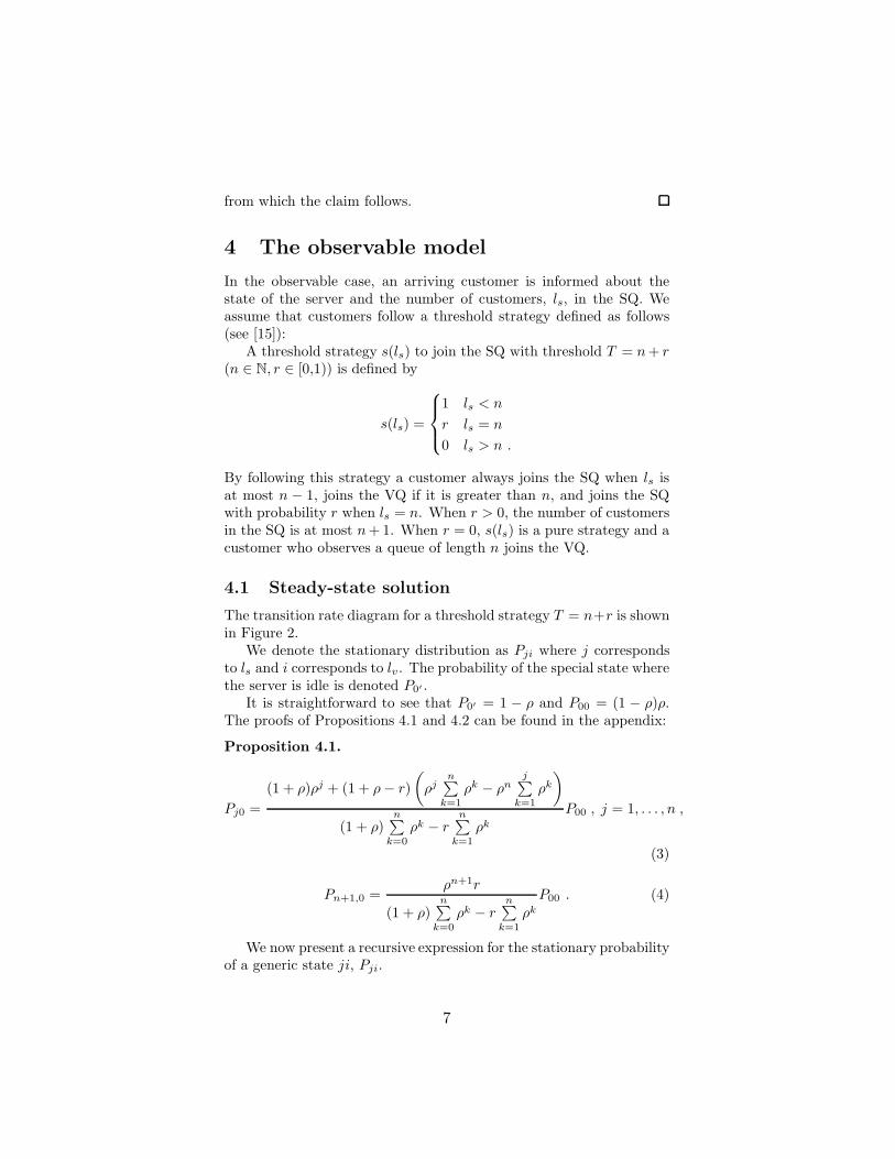
The transition rate diagram for a threshold strategy T = n+r is shownin Figure 2.

We denote the stationary distribution as Pji where j correspondsto ls and i corresponds to lv. The probability of the special state wherethe server is idle is denoted P0′ .

It is straightforward to see that P0′ = 1 − ρ and P00 = (1 − ρ)ρ.The proofs of Propositions 4.1 and 4.2 can be found in the appendix:

Proposition 4.1.

Pj0 =

(1 + ρ)ρj + (1 + ρ− r)

(

ρjn∑

k=1

ρk − ρnj∑

k=1

ρk)

(1 + ρ)n∑

k=0

ρk − rn∑

k=1

ρkP00 , j = 1, . . . , n ,

(3)

Pn+1,0 =ρn+1r

(1 + ρ)n∑

k=0

ρk − rn∑

k=1

ρkP00 . (4)

We now present a recursive expression for the stationary probabilityof a generic state ji, Pji.

7

0′ 0, 0 1, 0 . . . n, 0 n+1, 0

0, 1 1, 1 . . . n, 1 n+1, 1

0, 2 1, 2 . . . n, 2 n+1, 2

0, 3 1, 3 . . . n, 3 n+1, 3

. . . . . . . . . . . . . . .

ls

lv

λ λ λ λ

λ λ λ

λ λ λ

λ λ λ

λ

λ

λ

λ(1− r)

λ(1− r)

λ(1− r)

λr

λr

λr

λr

µ µ µ µ

µ µ µ

µ µ µ

µ µ µ

µ

µ

µ

µ

µ

µ

µ

Figure 2: Transition rate diagram in the observable model when customersfollow the mixed threshold strategy T = n+ r.

Proposition 4.2.

For i = 1, 2, . . . and 0 ≤ r < 1

Pni = XZi−1Pn+1,0 + Y Pn,i−1 +ρr

1 + ρXY

i−2∑

k=0

ZkPn,i−2−k , (5)

Pn+1,i =ρr

1 + ρY iPn0+ZPn+1,i−1+

ρr

1 + ρXY

i−2∑

k=0

Y kPn+1,i−2−k , (6)

Pji =

j∑

k=0

ρkP0i − (Pn+1,i + (1− r)Pni)

j∑

k=1

ρk , j = 1, 2, . . . , n− 1 ,

(7)P0i = (1− r)ρPn,i−1 + ρPn+1,i−1 , (8)

where

X =(1− ρn+2)ρ

(1 + ρ)(1− ρn+1)− (1− ρn)ρr, (9)

Y =(1− r)(1 + ρ)(1 − ρn+1)ρ

(1 + ρ)(1 − ρn+1)− (1− ρn)ρr, (10)

Z = (1 +Xr)ρ

1 + ρ. (11)

8

Remark 4.3. For i = 1 the sumsi−2∑

k=0

Y kPn+1,i−2−k andi−2∑

k=0

ZkPn,i−2−k

are over empty sets, therefore we have

Pn1 = Y Pn0 +XPn+1,0 , (12)

Pn+1,1 = ZPn+1,0 +ρr

1 + ρY Pn0 . (13)

Remark 4.4. The stationary probabilities of row i can be computedin O(n + i) time. By defining the functions

Fi =

i−2∑

k=0

ZkPn,i−2−k , F ′

i =

i−2∑

k=0

Y kPn+1,i−2−k

we have

Fi = Pn,i−2 + ZFi−1 , F ′

i = Pn+1,i−1 + Y F ′

i−1 ,

with this we express Pni and Pn+1,i as

Pni = XZi−1Pn+1,0 + Y Pn,i−1 +ρr

1 + ρXY Fi , (14)

Pn+1,i = ρrY iPn0 + ZPn+1,i−1 +ρr

1 + ρXY F ′

i . (15)

We first pre-calculate Y , Z, ρr1+ρ

XY , ρr1+ρ

Pn0 and XPn+1,0. Then wecalculate Pn,i and Pn+1,i and from these we calculate the probabilitiesPji j = 0, . . . , n. The pre-calculation is done in O(n) time by usingEquations (25), (4), (9), (10) and (11). We calculate Pn,i and Pn+1,i

by using Equations (15), (14) and the pre-calculated values. By savingthe variables Fk−1, F

′

k−1, Zk−2 and Y k−1 when we calculate Pnk and

Pn+1,k (0 < k < i) we can calculate Pn,k+1 and Pn+1,k+1 in O(1)time and therefore find Pn,i and Pn+1,i in O(i) time. We calculatethe stationary probabilities of the row using Equation (7). By savingthe value of the sums when calculating Pk−1,i we can find Pk,i in O(1)time and calculate all the stationary probabilities in O(n). Thereforethe calculation of a row i takes O(n + i) time.

For the SQ when the server is busy, the probability that the queuelength is ls is

P (ls) =

∑

∞

i=0Plsi

1− P0′.

and the expected queueing time of a customer joining it, given ls, is

E(Ws) =ls + 1

µ. (16)

9

The expected length of the VQ when the server is busy and thelength of the SQ is ls can be calculated from propositions 4.1, 4.2 andP (ls)

E(Lv|ls) =

∞∑

i=1

iPlsi

/

∞∑

i=0

Plsi . (17)

We define a busy-period type variable b(f), f = 0, . . . , n denoting theexpected time it takes the SQ to decrease its length from n+ 1− f ton − f . Similarly, b(n + 1) denotes the expected time it takes a busyserver to be ready to serve a customer from the VQ given that ls = 0.Then:

b(0) =1

µ,

b(1) =1

λ+ µ+

λr

λ+ µ(b(1) + b(0)) +

λ(1 − r)

λ+ µb(1) ,

b(f) =1

µ+ λ+

λ

µ+ λ(b(f) + b(f − 1)) f = 2, 3, . . . , n+ 1 .

These equations are explained as follows: When f = 0 new arrivals donot join the SQ and therefore b(0) = 1

µ. When f > 0, the expected

time until the next event is λ + µ. For f = 1, if the next event is anarrival then with probability r the arriving customer joins the SQ andneeds to wait b(0) and an additional b(1), and with probability 1 − rthe arriving customer joins the VQ and we stay at the same state.When f = 2, 3, . . . , if the next event is an arrival then we enter statef − 1 and need expected time b(f − 1) to return to state f and thenanother b(f) until the end of the busy period. If the next event is theend of service then the busy period terminates.

The solution to these equations is

b(1) =ρr + 1

µ,

b(f) =

(

f−1∑

k=0

ρk + ρfr

)

1

µ, f = 2, 3 . . . , n+ 1 . (18)

Finally, the expected queueing time of a customer who joins theVQ when the length of the SQ is ls is

E[W |ls] =

ls∑

k=0

b(n+ 1− k) + E(Lv|ls)b(n+ 1) , ls ≤ n+ 1 . (19)

The first term is the expected time until the server is ready to serve thefirst customer from the VQ, consisting of ls+1 consecutive busy periodswith increasing values of f , i.e., for the first busy period f = n+1− ls,

10

for the second f = n+1− (ls− 1), and so on, concluding with b(n+1)which is the time it takes until the first customer from the VQ is calledfor service given that the SQ is empty. The second term is the timeit takes until the server is ready to serve the new VQ customer giventhat it just started serving a VQ customer.

Remark 4.5. The case where the customers follow a pure strategy hasa closed-form solution:

Pn0 =ρn

n∑

k=0

ρkP00 , P01 =

ρn+1

n∑

k=0

ρkP00 ,

Pj0 =

ρjn∑

k=0

ρk − ρnj∑

k=1

ρk

n∑

k=0

ρkP00 , j = 1, . . . , n ,

Pji =ρn+i

n∑

k=0

ρkP00 ,

i = 1, 2, . . .j = 0, 1, . . . n ,

E(Lv|ls) =ρn+1

(

Pls0

n∑

k=0

ρk + ρn+2

)

(1− ρ)2P00 ,

and

E[W |ls] =

ls∑

k=0

b(n− k) + E(Lv|ls)b(n) , ls = 0, . . . , n .

4.2 Numerical investigation of the equilibrium strate-

gies

A complete analysis of the equilibrium strategies is not possible andtherefore we present in this section the results of a numerical study. Weconclude from this study that the conditional expected waiting timein the VQ is approximately linear and provide an explanation for thisphenomenon. This conclusion enables us to obtain important insightsabout the equilibrium behavior. Specifically we provide conditions fordominant strategies, and show that when these conditions are violatedthere are, in general, multiple equilibrium solutions.

We define the normalized expected waiting time in the VQ

E[W |ls] =E[W |ls]

1

µ

=

ls∑

k=0

b′(n+1−k)+E(Lv|ls)b′(n+1) , ls ≤ n+1 .

(20)

11

0 2 4 6 8 10 12 14 160

10

20

30

40

50

60

70

T = 5

ls

l s ∑ k=0

b′(n

+1−k)

ρ = 0.8

T = 5.6

T = 6.2 T = 6.8

T = 7.4 T = 8

T = 8.6

T = 9.2 T = 9.8

T = 10.4 T = 11

T = 11.6

T = 12.2 T = 12.8

T = 13.4 T = 14

T = 14.6

T = 15.2 T = 15.8

Figure 3:ls∑

k=0

b′(n+ 1− k) when ρ = 0.8.

0 2 4 6 8 10 12 14 160

5

10

15

20

25

T = 5

ls

E(L

q v|ls)b

′ (n+

1)

ρ = 0.8

T = 5.3 T = 5.6 T = 5.9

T = 9

T = 9.3 T = 9.6 T = 9.9 T = 13

T = 13.3

T = 13.6

T = 13.9 T = 15

T = 15.3

T = 15.6

T = 15.9

Figure 4: E(Lv |ls)b′(n+ 1) when ρ = 0.8.

12

0 2 4 6 8 10 12 14 160

10

20

30

40

50

60

70

80

90

T = 5

ls

E(W q)

ρ = 0.8

T = 5.6 T = 6.2

T = 6.8 T = 7.4

T = 8

T = 8.6 T = 9.2

T = 9.8 T = 10.4

T = 11

T = 11.6 T = 12.2

T = 12.8 T = 13.4

T = 14

T = 14.6

T = 15.2

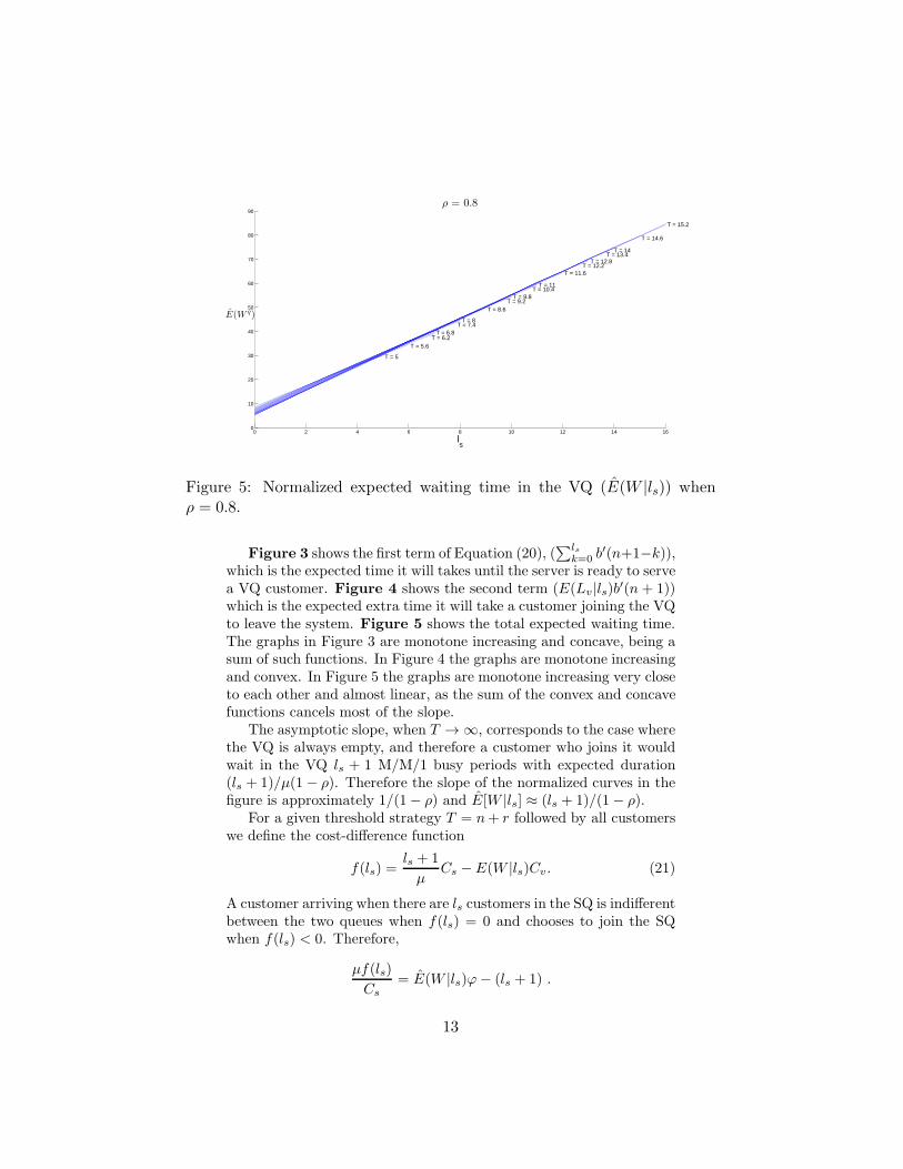
Figure 5: Normalized expected waiting time in the VQ (E(W |ls)) whenρ = 0.8.

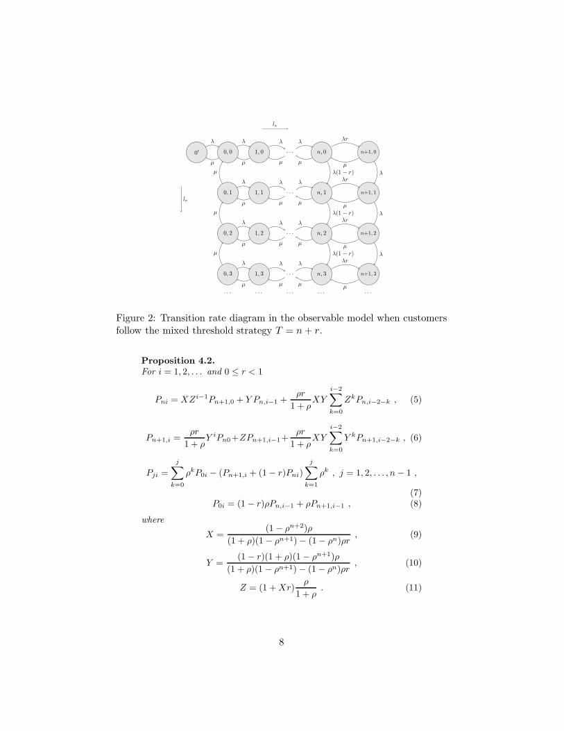
Figure 3 shows the first term of Equation (20), (∑ls

k=0b′(n+1−k)),

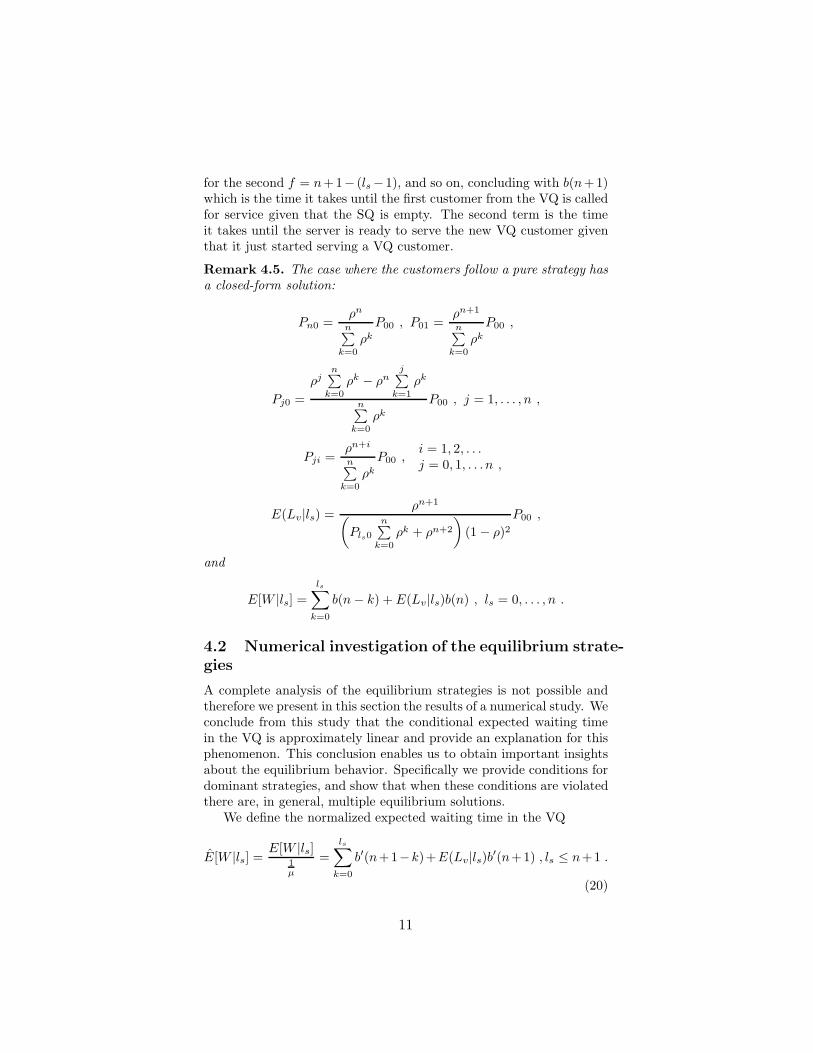
which is the expected time it will takes until the server is ready to servea VQ customer. Figure 4 shows the second term (E(Lv|ls)b

′(n+ 1))which is the expected extra time it will take a customer joining the VQto leave the system. Figure 5 shows the total expected waiting time.The graphs in Figure 3 are monotone increasing and concave, being asum of such functions. In Figure 4 the graphs are monotone increasingand convex. In Figure 5 the graphs are monotone increasing very closeto each other and almost linear, as the sum of the convex and concavefunctions cancels most of the slope.

The asymptotic slope, when T → ∞, corresponds to the case wherethe VQ is always empty, and therefore a customer who joins it wouldwait in the VQ ls + 1 M/M/1 busy periods with expected duration(ls + 1)/µ(1− ρ). Therefore the slope of the normalized curves in thefigure is approximately 1/(1− ρ) and E[W |ls] ≈ (ls + 1)/(1− ρ).

For a given threshold strategy T = n+ r followed by all customerswe define the cost-difference function

f(ls) =ls + 1

µCs − E(W |ls)Cv. (21)

A customer arriving when there are ls customers in the SQ is indifferentbetween the two queues when f(ls) = 0 and chooses to join the SQwhen f(ls) < 0. Therefore,

µf(ls)

Cs

= E(W |ls)ϕ− (ls + 1) .

13

0 5 10 15 200

2

4

6

8

10

12

14

16

18

ls

Cos

t

ρ = 0.4

SQ Cost

VQ Cost

0 5 10 15 200

2

4

6

8

10

12

14

16

18

ls

Cos

t

ρ = 0.6

SQ Cost

VQ Cost

0 5 10 15 200

2

4

6

8

10

12

14

16

18

ls

Cos

t

ρ = 0.8

SQ Cost

VQ Cost

Figure 6: Cost of joining the SQ and cost in the VQ for 5 ≤ T ≤ 15 andϕ = 0.2

Substituting E(W |ls) ≈ (ls + 1)/(1− ρ) gives

µf(ls)

Cs

≈ (ls + 1)

(

ϕ

1− ρ− 1

)

. (22)

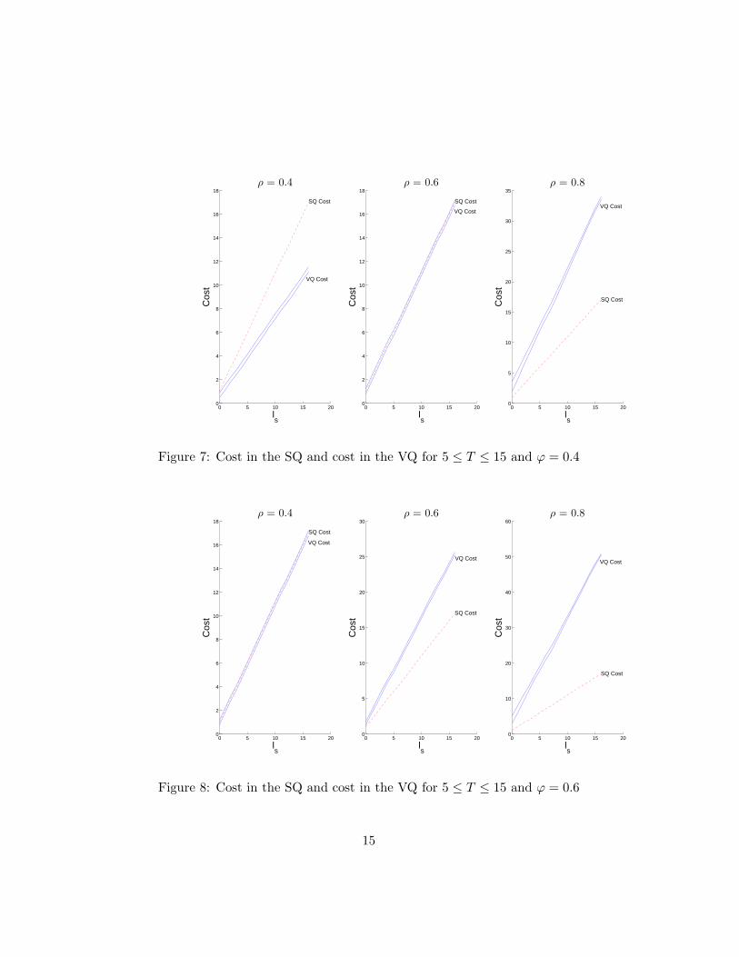
Figures 6-8 show the two cost components of Equation (21) ineach of the queues for different values of ϕ and ρ. The VQ costs arealmost linear in ls and very close to each other for close values of T ,in accordance to the VQ expected waiting times shown in Figure 5.Therefore we have marked the area in the graph were all the VQ costsreside by two solid lines. The broken line is the expected cost associatedwith joining the SQ. When the VQ cost area is above the SQ cost line,the cost of joining the SQ is always smaller than the cost of joining theVQ and therefore all arriving customers will join the SQ regardless ofits size. As one expects from Equation (22), this case occurs when ϕ issignificantly greater than 1− ρ. Customers will always join the VQ inthe opposite case, when ϕ is significantly smaller than 1−ρ. When theSQ line passes the VQ costs area or resides inside it there are values ofT for which f(ls) = 0 and therefore are candidates to be equilibriumstrategies. This case is obtained when ϕ ≈ 1 − ρ, because, as impliedby Equation (22), in this case the expected waiting times at the SQand the VQ are approximately equal. For example, in Figure 7, whenρ = 0.4 joining the VQ is a dominating strategy, when ρ = 0.8 joining

14

0 5 10 15 200

2

4

6

8

10

12

14

16

18

ls

Cos

t

ρ = 0.4

SQ Cost

VQ Cost

0 5 10 15 200

2

4

6

8

10

12

14

16

18

ls

Cos

t

ρ = 0.6

SQ Cost

VQ Cost

0 5 10 15 200

5

10

15

20

25

30

35

ls

Cos

t

ρ = 0.8

SQ Cost

VQ Cost

Figure 7: Cost in the SQ and cost in the VQ for 5 ≤ T ≤ 15 and ϕ = 0.4

0 5 10 15 200

2

4

6

8

10

12

14

16

18

ls

Cos

t

ρ = 0.4

SQ Cost

VQ Cost

0 5 10 15 200

5

10

15

20

25

30

ls

Cos

t

ρ = 0.6

SQ Cost

VQ Cost

0 5 10 15 200

10

20

30

40

50

60

ls

Cos

t

ρ = 0.8

SQ Cost

VQ Cost

Figure 8: Cost in the SQ and cost in the VQ for 5 ≤ T ≤ 15 and ϕ = 0.6

15

0 1 2 3 4 5 6 7 8−0.2

−0.1

0

0.1

0.2

0.3

0.4

0.5

0.6

T = 7.05

ls

Cos

t Diff

eren

ce

ρ = 0.8

T = 7.14 T = 7.2 T = 7.3 T = 7.4

Figure 9: Expected cost difference SQ−VQ for thresholds T = 7 + r, r =(0.05, 0.14, 0.2, 0.3, 0.4), ϕ = 0.2 and ρ = 0.8.

the SQ dominates, and when ρ = 0.6 we have ϕ = 1−ρ and (multiple)non-dominating equilibria exist.

We search for best response and equilibrium best response strate-gies for a given n by looking at the expected cost-difference graph.Figure 9 plots the expected cost difference (SQ-VQ), a horizontal lineat y = 0 and a vertical line x = n for n = 7. In a pure equilibriumthe cost-difference function is negative at n − 1 and positive at n. Ina mixed equilibrium it is zero at n, as obtained for T ≈ 7.14 in thefigure.

Figures 10-12 show the best response for three pairs (ρ, ϕ = 1−ρ). As explained above, we expect non-dominating equilibria for suchpairs. The intersection of the best response function and the 45◦ lineare either equilibrium points or points at the end of the action space.For example, for ϕ = 0.2, ρ = 0.8 (Figures 10), if all others use athreshold T = 1 then the queue length is at most 2 and the bestresponse of a customer is to join even when arriving to a system queueof this length. Thus T = 1 is not an equilibrium. The pure equilibriaare at T = 3, . . . , 12 and between every two pure equilibria n and n+1there is a mixed equilibrium n + r for some 0 < r < 1. (The firstones are difficult to observe in the figure as r is close to 0.) Thesemixed solutions occur at the intersection of the 45◦ line with a vertical“jump” of the best response function, indicating indifference between

16

0 5 10 15 20 250

5

10

15

20

25

BR

T

Bes

t Res

pons

e

ρ = 0.8

Figure 10: Best response for ϕ = 0.2, ρ = 0.8

0 5 10 15 20 250

5

10

15

20

25

BR

T

Bes

t Res

pons

e

ρ = 0.6

Figure 11: Best response for ϕ = 0.4, ρ = 0.6

0 5 10 15 20 250

5

10

15

20

25

BR

T

Bes

t Res

pons

e

ρ = 0.4

Figure 12: Best response for ϕ = 0.6, ρ = 0.4

17

two integer thresholds. In Figure 11 the pure equilibria are 12, . . . , 17,and in Figure 12 they are 15, . . . , 18.

The best response functions are increasing and then decreasing inls which reflect follow-the-crowd (FTC) and avoid the crowd (ATC)strategies respectively. FTC behavior is common in priority queues,but in our case when the threshold adopted by others is very highthe individual prefers not to compete with them and joins the SQinstead. Another example of such behavior has been found by Havivand Ravner [20] while investigating an accumulating priority queuesystem with different costs per unit time per customer class.

5 Concluding remarks

We investigated a non-preemptive single-server M/M/1 system with aSystem Queue (SQ) and a Virtual Queue (VQ). When the server isbusy an arriving customer chooses between joining the VQ or the SQ.Waiting in the VQ is less costly. In the unobservable case customers arenotified only whether the server is busy or not, and in the observablecase they are also informed about ls, the number of customers in theSQ.

For each case we compute the expected waiting time in each of thequeues and the equilibrium joining strategy of an arriving customer.In the observable case, the conditional expected waiting time in theVQ turns out to be almost linear in ls. We use this fact to charac-terize the equilibrium behavior, that shows similarities to that of theunobservable case. Multiple equilibrium strategies may exist, all inthe monotone increasing part of the best response function, and thisis compatible with a follow-the-crowd (FTC) behavior.

Clearly, since the customers’ joining strategy has no effect on theirexpected waiting time, it is socially optimal, in both models, that allcustomers join VQ, and a social planner would encourage all the cus-tomers to join the VQ. This can be done in many ways involving penal-ties, subsidies, or a change in the service priority regime.

Our motivation for investigating service systems with virtual queuesarises from call centers and similar systems where reaching VQ cus-tomers is practically costless and instantaneous. We believe howeverthat analyzing similar systems in which contacting a customer fromthe VQ requires non-negligible time or expenditure is an interestingdirection for future research. Such a system, but without an SQ, issolved by Economou and Kanta [12]. Another interesting variation ofour model would allow customers to move from one queue to the other.

18

References

[1] Adiri, I. and U. Yechiali, (1974) Optimal priority-purchasing andpricing decisions in nonmonopoly and monopoly queues, Opera-tions Research 22, 1051–1066.

[2] Aguir, M.S., F. Karaesmen, O.Z. Aksin, and F. Chauvet, (2004)The impact of retrials on call center performance, OR Spectrum26, 353–376.

[3] Altman, E., T. Jimenez, R. Nunez-Queija, and U. Yechiali, (2004)Optimal routing among ·/M/1 queues with partial information,Stochastic Models 20, 149–171.

[4] Armony, M. and C. Maglaras, (2004) On customer contact cen-ters with a call-back option: customer decisions, routing rules, andsystem design, Operations Research, 52, 271–292.

[5] Armony, M. and C. Maglaras, (2004) Contact centers with a call-back option and real-time delay information, Operations Research,52, 527–545.

[6] Burgain, P., E. Feron, and J.-P Clarke, (2009) Collaborative virtualqueue: benefit analysis of a collaborative decision making conceptapplied to congested airport departure operations, Air Traffic Con-trol Quarterly 17, 195–222.

[7] Camulli, E., (2007) Answer my call: technology helps utilities getcustomers off hold, Electric Light and Power 2, 56.

[8] Chakravarthy, R.S., A. Krishnamoorthy, and V.C. Joshua, (2006)Analysis of a multi-server retrial queue with search of customersfrom the orbit, Performance Evaluation, 63, 776–798.

[9] Cooper, B.R., (1981) Introduction to Queueing Theory - SecondEdition, North Holland.

[10] Cope III, R.F., R.F. Cope and H.E. Davis, (2008) Disney’s virtualqueues: a strategic opportunity to co-brand services?, Journal ofBusiness and Economics Research 6, 13–20.

[11] Dickson, D., R.C. Ford, and B. Laval, (2005) Managing real andvirtual waits in hospitality and service organizations, Cornell Hoteland Restaurant Administration Quarterly, 46, 52–68.

[12] Economou, A. and S. Kanta, (2011) Equilibrium customer strate-gies and social-profit maximization in the single-server constantretail queue, Naval Research Logistics 58, 107–122.

[13] Edelson, N.M. and K. Hildebrand, (1975) Congestion tolls forPoisson queuing processes, Econometrica 43, 81–92.

[14] Guijarro, L., V. Pla, and B. Tuffin, (2013) Entry game underopportunistic access in cognitive radio networks: a priority queuemodel, Wireless Days (WD), 1–6.

19

[15] Hassin, R., (1996)On the advantage of being the first server, Man-agement Science, 42, 618–623.

[16] Hassin, R., (2016) Rational Queueing, CRC Press.

[17] Hassin, R. and M. Haviv, (1997) Equilibrium threshold strategies:the case of queues with priorities, Operations Research, 45, 966–973.

[18] Hassin, R. and M. Haviv, (2003) To Queue or Not to Queue: Equi-librium Behavior in Queueing Systems, Kluwer Academic Publish-ers

[19] Haviv, M., (2013) Queues - A Course in Queueing Theory,Springer-Verlag, 191.

[20] Haviv, M. L. and Ravner, (2016) Strategic bidding in an accumu-lating priority queue: equilibrium analysis, Annals of OperationsResearch (to appear).

[21] Iravani, F. and B. Balcioglu, (2008) On priority queues with im-patient customers, Queueing Systems, 58, 239–260.

[22] Kopzon, A., Y. Nazarathy, and G. Weiss, (2009) A push pullqueueing with infinite supply of work, Queueing Systems: Theoryand Applications, 66, 75–111.

[23] Kostami, V. and R.A. Ward, (2009) Managing service systemswith an offline waiting option and customer abandonment, Manu-facturing & Service Operations Management 11, 644–656.

[24] de Lange, R., I. Samoilovich, and B. van der Rhee, (2013) Virtualqueuing at airport security lanes, European Journal of OperationalResearch 225, 153–165.

[25] Lovejoy, T.C., S. Aravkin, and C. Schneider-Mizell, (2004)Kalman queue: an adaptive approach to virtual queuing, TheUMAP Journal 25, 337–352.

[26] Mandelbaum, A. and U. Yechiali, (1983) Optimal entering rulesfor a customer with wait option at an M/G/1 queue, ManagementScience, 29, 174–187.

[27] Naor, P., (1969) The regulation of queue size by levying tolls,Econometrica 37, 15–24.

[28] Littlechild, S.C., (1974) Optimal arrival rate in a simple queueingsystem, International Journal of Production Research 12, 391–397.

[29] Wuchner, P., J. Sztrik, and H. de Meer, (2009) Finite-sourceM/M/S retrial queue with search for balking and impatient cus-tomers from the orbit, Computer Networks 53, 1264–1273.

20

Appendix: Notations and proofs

Notations and Definitions

SQ System queue.VQ Virtual queue.Cs, Cv Waiting costs in the SQ and VQ.

ϕ The cost ratio, ϕ = Cv

Cs

.

λ Mean arrival rate of customers to the system.µ Mean service rate.rs Probability of joining the SQ in the unobservable case.S(rs) Expected net benefit for a customer following the strategy rs.Ls(t), Lv(t) The number of customers in SQ and the VQ at time t.E(L), E(Ws), E(Wv) Expected waiting time in the system, SQ and VQ, respectively.

E[W |ls] The expected waiting time in the VQ in time units per customer.E(Ls), E(Lv) Expected number of customers in the SQ and VQ.ρ, ρs, ρv Occupation rates in the entire system, the SQ and the VQ.P Stationary probabilities.ls Number of customers in the SQ.s(ls) Threshold strategy of joining the SQ.T Threshold strategy, T = n+ r (r ∈ [0, 1], n ∈ N).f Number of unoccupied places in the SQb(f) Mean busy period when there are n+ 1− f customers in the SQ.b′(f) Normalized b(f).

Proof of Proposition 4.1 From the transition rate diagram

(λ+ µ)Pn+1,0 = λrPn0

and thereforePn+1,0 =

ρr

ρ+ 1Pn0 . (23)

A cut around nodes 0′, 00, 10, . . . , j0 gives

λPj0 = µP01 + µPj+1,0 , j = 0, 1, . . . , n ,

or, after reindexing,Pj0 = ρPj−1,0 − P01.

We now substitute P01 from the upper horizontal cut equation

λ(1 − r)Pn0 + λPn+1,0 = µP01

and Pn+1,0 from (23) and obtain

Pj0 = ρPj−1,0 −1 + ρ− r

1 + ρρPn0 , j = 1, . . . , n+ 1 .

21

A recursive application of this equation gives

Pj0 = ρjP00 −1 + ρ− r

1 + ρPn0

j∑

k=1

ρk , j = 1, . . . , n+ 1 . (24)

Specifically for j = n

Pn0 = ρnP00 −1 + ρ− r

1 + ρPn0

n∑

k=1

ρk ,

giving

Pn0 =(1 + ρ)ρn

(1 + ρ)n∑

k=0

ρk − rn∑

k=1

ρkP00 . (25)

Substituting Pn0 in (23) gives (4).From Equations (25) and (24) we obtain

Pj0 = ρjP00 −1 + ρ− r

1 + ρ

(1 + ρ)ρn

(1 + ρ)n∑

k=0

ρk − rn∑

k=1

ρk

j∑

k=1

ρkP00

which gives (3).

Proof of Proposition 4.2

Equation (8) follows from the horizontal cut between the rows i, i−1

λ(1− r)Pni + λPn+1,i = µP0,i+1 , i = 0, 1, 2, . . . . (26)

A cut that contains the nodes 0i, 1i, . . . , ji gives

λPji + µP0i = µPj+1,i + µP0,i+1

i = 1, 2, . . .j = 0, 1, 2, . . . , n− 1 .

(27)

By Equation (26) and re-indexing we have

Pji = P0i − (1 − r)ρPni − ρPn+1,i + ρPj−1,ii = 1, 2, . . .j = 1, 2, . . . , n

.

A recursive application of this relation leads to Equation (7).We now find an expression for Pni and Pn+1,i. Equation (7) for Pni

yields[

n∑

k=0

ρk − r

n∑

k=1

ρk

]

Pni =

n∑

k=0

ρkP0i −

n∑

k=1

ρkPn+1,i , (28)

and the cut around the node (n+ 1)i is

(1 + ρ)Pn+1,i = ρPn+1,i−1 + ρrPni . (29)

22

By Equations (8), (28) and (29) we have

Pni =

(1 + ρ)(1 − r)n+1∑

k=1

ρk

n+1∑

k=1

ρk +n∑

k=0

ρk − rn∑

k=1

ρkPn,i−1+

n+2∑

k=1

ρk

n+1∑

k=1

ρk +n∑

k=0

ρk − rn∑

k=1

ρkPn+1,i−1 .

(30)With this result and Equation (29) we also get

Pn+1,i =

1 +

ρrn+2∑

k=1

ρk

n+1∑

k=1

ρk +n∑

k=0

ρk − rn∑

k=1

ρk

ρ

ρ+ 1Pn+1,i−1

+

(1 + ρ)(1− r)rn+2∑

k=2

ρk

n+1∑

k=1

ρk +n∑

k=0

ρk − rn∑

k=1

ρkPn,i−1 .

(31)

In terms of X,Y, Z as defined in Equations (9) - (11) we have

Pni = Y Pn,i−1 +XPn+1,i−1 , Pn+1,i = ZPn+1,i−1 +ρr

1 + ρY Pn,i−1

therefore

Pni = Y iPn0 +X

i−1∑

k=0

Y kPn+1,i−1−k ,

Pn+1,i = ZiPn+1,0 +ρr

1 + ρY

i−1∑

k=0

ZkPn,i−1−k

and we get (5) and (6).

23