customer acquisition, retention, and service access quality
TRANSCRIPT

Customer Acquisition, Retention, and Service Access Quality:
Optimal Advertising, Capacity Level and Capacity Allocation
Philipp Afèche
Rotman School of Management, University of Toronto
Mojtaba Araghi
School of Business and Economics, Wilfried Laurier University
Opher Baron
Rotman School of Management, University of Toronto
December 2016
(1) Problem Definition: We provide guidelines on three fundamental decisions of customer relation-
ship management (CRM) and capacity management for profit-maximizing service firms that serve heteroge-
neous repeat customers, whose acquisition, retention, and behavior depend on their service access quality to
bottleneck capacity: How much to spend on customer acquisition, how much capacity to deploy, and how to
allocate capacity and tailor service access quality levels to different customer types.
(2) Academic / Practical Relevance: These decisions require a clear understanding of the con-
nections between customers’ behavior and value, their service access quality, and the capacity allocation.
However, existing models ignore these connections.
(3) Methodology: We develop and analyze a novel fluid model that accounts for these connections.
Simulation results suggest that the fluid-optimal policy also yields near-optimal performance for large sto-
chastic queueing systems with abandonment.
(4) Results: First, we derive new customer value metrics that extend the standard ones by accounting
for the effects of the capacity allocation, the resulting service access qualities and customer behavior: A
customer’s lifetime value; her index, where is her one-time service value and her service rate; and her
policy-dependent value which reflects the indices of other served types. Second, we link these metrics to
the profit-maximizing policy and to new capacity management prescriptions, notably, optimality conditions
for rationing capacity and for identifying which customers to deny service. Further, unlike standard index
policies, the optimal policy prioritizes customers based not on their indices, but on policy- and type-
dependent functions of these indices.
(5) Managerial Implications: First, our study highlights the importance of basing decisions on more
complete metrics that link customer value to the service access quality; marketing-focused policies that
ignore these links may reduce profits significantly. Second, the proposed metrics provide guidelines for
valuing customers in practice. Third, our decision guidelines help managers design more profitable policies
that effectively integrate CRM and capacity management considerations.
1 Introduction
Many service firms serve heterogeneous repeat customers whose acquisition, retention, and behavior
during their lifetime in the customer base depend on their service quality. A key dimension of
service quality is access to bottleneck capacity, such as call centers, field operations, or fulfillment
operations. We study three interrelated strategic decisions for a profit-maximizing firm in this
situation: how much to spend on new customer acquisition, how much capacity to deploy, and how
to allocate this capacity and tailor service access quality levels to different customer types.
1

This problem was motivated by several questions that emerged in our conversations with man-
agers of a credit card company on how to manage customer access to its call center. What is the
value of a call and the lifetime value of a customer? What are the effects of the service access
quality on these metrics? How should the optimal decisions consider these effects, and what are
the consequences of ignoring them? These questions highlight the importance of considering the
effects of service access quality on the overall customer relationship, not only on individual calls,
consistent with the key premise of customer relationship management (CRM). The importance of
a CRM approach to call center capacity management is supported by customer surveys and other
researchers. As Anton et al. (2004) estimate, firms that use call centers conduct 80% of interactions
with their customers through this channel, and 92% of customers base their opinion of a company
on their call center service experiences. Moreover, these experiences can have a dramatic impact
on customer satisfaction and retention. Long waiting times are cited by 67% of customers as a
major cause of frustration, and a poor call center experience is cited by 40% of customers as the
sole reason for terminating their relationship with a business (Genesys Global Consumer Survey
2007). According to Aksin et al. (2007, p. 682) “firms would benefit from a better understand-
ing of the relationship between customers’ service experiences and their repeat purchase behavior,
loyalty to the firm, and overall demand growth in order to make better decisions about call center
operations.” The importance of understanding this relationship for call centers has recently also
been recognized in the marketing literature (cf. Sun and Li 2011).
This paper provides a foundation for building such understanding, based on a new fluid model
that integrates CRM and service operations management. Whereas the call center context moti-
vated this research, our model emphasizes general features that apply to any bottleneck capacity
of a service firm. For instance, at a high level Amazon.com faces a similar problem to allocate its
fulfillment capacity between new customers, Prime customers, and non-Prime customers.
We model homogeneous new customers and heterogeneous base (repeat) customer types that
differ in their service request rates, service-dependent and -independent profits and costs, and reac-
tions to their service access quality, measured by their service probability. The firm uses advertising
to control new customer arrivals, and the capacity level and allocation to control customers’ service
probabilities and in turn, their customer base transitions — from conversion to base customers of
different types, to switching among types, to defection. The novelty of this model is to link the
makeup and value of the customer base both to the capacity allocation, unlike prior CRM models,
and to the service access quality of past interactions, unlike prior capacity management models.
This paper makes the following contributions to CRM and service capacity management.
1. Customer value metrics that depend on the capacity allocation policy. We identify novel
metrics that, unlike standard ones, link the value of a customer to the capacity allocation policy
and the resulting service probabilities and customer base transitions of all types: () The customer
lifetime value (CLV) of base customers. () The index of a customer type, where is her
one-time service value (OTV) and her service rate. A type’s index depends on the CLVs and
quantifies the value generated by allocating one unit of capacity to serving that type, including her
instant service-dependent profit plus the expected future service-independent profits of the types
that she may switch to. () The policy-dependent value of a customer type, which reflects not
only her own index, but also the indices of the served types that she may switch to.
2

2. Guidelines for service capacity management. We contribute () new analytical prescriptions
for and () important implications that follow from, the profit-maximizing advertising, capacity,
and capacity allocation policies. () The optimal capacity allocation policy in our model features
two key differences to standard index policies: first, the indices consider the effect of service
on customers’ future requests and financial impact; second, since the value of serving a type also
depends on the indices of other types, customers’ optimal priority ranking does not correspond
to that of their indices. Furthermore, we find that under mild conditions it is optimal to ration
capacity, whereby the firm serves only new and lucrative base customers, but denies service to
unprofitable base customers. We derive optimality conditions for capacity rationing, first for the
case where base customers’ service quality only affects their retention, then for cases where they also
respond to service quality by switching their type or by spreading negative word of mouth. () Our
results have a number of important implications. First, the customer attributes may have subtle
effects on the optimal policy. The flexibility of our model allows managers to account for these
effects. Second, in settings with repeat customers the capacity allocation policy plays a key role
— previously ignored — in controlling the customer base composition through differentiated service
levels. Third, marketing-focused policies that ignore the effect of service probabilities on the CLV
may yield suboptimal decisions and reduce profits significantly. Finally, simulation results show
that the optimal policy in the fluid model also yields near-optimal performance in a corresponding
stochastic many-server queueing model with abandonment. This suggests that our fluid model
approach may prove effective in tackling further problems of joint CRM and capacity management
for stochastic service systems, such as the credit card call center that motivated this research.
In §2 we review the related literature. In §3 we present the model and problem formulation.
In §4 we develop the main results for the case without base customer switching. In §5 we discuss
how these results generalize under base customer type switching and under word of mouth about
service quality. In §6 we discuss the implications of our results. In §7 we offer concluding remarks.
All proofs and certain derivations are in the online supplement.
2 Literature Review
This paper bridges research streams on advertising, CRM, service capacity management to serve
demand that is independent of past service quality, and operations management to serve demand
that depends on past service quality.
Advertising. The vast majority of papers on advertising, unlike ours, ignore supply constraints.
Feichtinger et al. (1994) offer an extensive review. Papers that do consider supply constraints study
different settings; e.g., in Sethi and Zhang (1995) demand is independent of past service quality, in
Olsen and Parker (2008) customers are homogeneous, both studies consider systems with inventory.
CRM. Models of CRM and CLV are of central concern in marketing. For reviews see Rust
and Chung (2006) and Reinartz and Venkatesan (2008) on CRM, and Gupta et al. (2006) on
CLV. Studies that propose and empirically demonstrate the value of CLV-based frameworks for
customer selection and marketing resource allocation include Rust et al. (2004) and Venkatesan
and Kumar (2004). Based on the CLV components, CRM initiatives can be classified as focusing
on customer acquisition, growth, and/or retention. Studies that focus on the relationship between
3

acquisition and retention spending include Blattberg and Deighton (1996), Reinartz et al. (2005),
Musalem and Joshi (2009), Pfeifer and Ovchinnikov (2011) and Ovchinnikov et al. (2014). Studies
that focus on the effects of marketing actions on customer growth include Bitran and Mondschein
(1996), Lewis (2005), Li et al. (2005), Rust and Verhoef (2005), and Günes et al. (2010). Papers
that focus on explaining or predicting customer retention and churn include Verhoef (2003), Braun
and Schweidel (2011), and Ascarza and Hardie (2013). Studies that link service quality, customer
satisfaction, retention and other CLV components include Anderson and Sullivan (1993), Rust et
al. (1995), Zeithaml et al. (1996), Bolton (1998), Ho et al. (2006) and Aflaki and Popescu (2014).
Compared to the CRM literature, the key distinction of our model is that we explicitly link
customer acquisition and retention to the capacity-allocation-dependent service quality. Studies
that optimize some notion of service quality (Ho et al. 2006 and Aflaki and Popescu 2014) ignore
capacity constraints (and customer acquisition). The papers that consider a capacity constraint
(Pfeifer and Ovchinnikov 2011 and Ovchinnikov et al. 2014) study a firm’s optimal spending on
customer acquisition and retention of two base customer types (“low” and “high”) that do not
switch. However, their models ignore the link between capacity allocation and service quality: All
base customers are served in each period, whereas their retention depends on the firm’s spending.
These models are therefore not equipped to study the design of optimal capacity allocation policies,
and unlike our model cannot yield optimal capacity rationing in the absence of uncertainty.
Service capacity management to serve demand that is independent of past service quality. There
is a vast literature on service capacity management. Capacity allocation studies consider operational
tools including admission, priority and routing controls, marketing controls such as cross-selling
and pricing, or a combination of both. Call centers are among the most extensively studied service
systems. Gans et al. (2003), Aksin et al. (2007), and Green et al. (2007) survey the call center
literature. Hassin and Haviv (2003) and Hassin (2015) survey the literature on managing queueing
systems with rational customers. These research streams focus on service access quality, i.e, waiting
time and/or abandonment, assuming a fixed and perfect service delivery quality. However, there
is growing interest in considering service delivery failures (e.g., de Véricourt and Zhou 2005) or
trade-offs between the service delivery quality and waiting time (e.g., Anand et al. 2011).
In contrast to this paper, these research streams model a firm’s customer base as independent
of the capacity allocation policy and the service quality of past interactions. That is, they model the
arrivals of potential customer requests as exogenous but allow the outcomes of these requests (such
as balking, retrial, abandonment, or spending amount) to depend on the service quality. Because
these models do not keep track of repeat customers, their service level prescriptions reflect only
transaction-based metrics such as waiting and abandonment costs. In contrast, the prescriptions
in our model also consider the effect of service levels on customers’ future demand and their CLV.
Operations management to serve demand that depends on past service quality. A number of
papers consider the link between demand and past service quality with a different focus from
ours. Schwartz (1966) appears to be the first to consider how demand depends on past inventory
availability. Gans (2002) and Bitran et al. (2008b) consider a general notion of service quality in
the absence of capacity constraints, the former for oligopoly suppliers, the latter for a monopoly.
Hall and Porteus (2000), Liu et al. (2007), Gaur and Park (2007), and Olsen and Parker (2008)
study equilibrium capacity/inventory control strategies and market shares of firms that compete for
4

customers who switch among them in reaction to poor service. These papers, unlike ours, consider
homogeneous customers and a single service level for each firm. Sun and Li (2011) empirically
estimate how retention depends on customers’ allocation to on- vs. off-shore call centers, and on
waiting and service time. Their results underscore the value of modeling the link between these
service quality metrics, retention and CLV. Farzan et al. (2012) consider a FIFO queue with repeat
purchases that depend on past service quality, but quality is independent of the capacity allocation,
unlike in our model. Adelman and Mersereau (2013) study the dynamic capacity allocation problem
of a supplier with a fixed set of heterogeneous customers whose demands depend on their past fill
rates. In their model, past service quality affects customers’ profitability, not their retention.
3 Model and Problem Formulation
The credit card company that motivated this research uses call centers as the main customer contact
channel. The firm also uses other channels such as the web, e-mail, and SMS, but these are much
less costly and less suited for requests that require interaction with customer service representatives.
The focus of our model, one of the firm’s call centers, is both sales- and service-oriented.
Potential new customers call in response to advertised credit card offers. Existing card holders call
with service requests, e.g., to increase their credit limit, report a lost or stolen card, and so on.
Marketing and operations decisions are made each month according to the following procedure.
The marketing department sets the monthly advertising spending level and the volume of credit
card offers to be mailed out, based on some measures of customer profitability. The operations
department is not involved in these decisions, and they ignore operational factors, specifically,
service level considerations and staffing cost. Once the monthly advertising level is determined,
credit card offers are mailed evenly over the course of that month.
Following the advertising decisions, the operations department forecasts the monthly call volume
based on a number of factors, including the number of offers to be mailed to new customers and
historical data on their demand response, and the number and calling pattern of base customers.
Based on the monthly call volume forecast, the operations department determines the staffing
level for that month to meet certain predetermined service level targets.
This decision procedure raises the following issues: 1. There is no clarity about the value of a
call, the value of a customer, and how these measures depend on the call center’s service quality.
2. Advertising and staffing decisions either ignore service level considerations or make arbitrary
assumptions about service level targets. 3. It is not clear whether to prioritize certain customers,
and if so, on what basis. 4. Marketing and operations do not adequately coordinate their decisions.
These issues are pertinent not only for this company, but also for other firms facing the challenge
of how to manage costly capacity in serving heterogeneous customers. To address these issues, in
§3.1 we develop a deterministic fluid model that captures the strategic marketing and operations
tradeoffs. In §3.2 we discuss the model assumptions. In §6.4 we show that this model also closely
approximates large-scale stochastic queueing systems such as the credit card company’s call center.
5

3.1 The Model
Consider a firm that serves new and base (i.e., existing) customers with some service capacity.
Following their first interaction with the firm, new customers may turn into any of base customer
types. Base customers make up the firm’s customer base and repeatedly interact with the firm.
We index new customers by = 0, base customers by ∈ {1 2 }, say type- customers when ∈ {0 1 2 }, and type- base customers when ∈ {1 2 }. Service requests arrive asdetailed below. Let denote the service rate for type- requests. Table 1 summarizes the notation.
We consider the system in steady-state under three stationary controls. The advertising policy
controls the new customer arrival rate 0 as detailed below. The capacity policy controls the
capacity , defined as the total processing time available per unit time, at a unit cost per unit
time (in a call center corresponds to the number of servers). The capacity allocation policy
controls the service probabilities: Let the decision variable denote the steady-state type- service
probability and q:= (1 ) the 1× vector of base customer service probabilities.
Decision Variables
Capacity
0 Arrival rate of new customers
Service probability of type- customers
System Parameters
Service rate of type- customers
Arrival rate per type- base customer
() probability that a type- customer, served with probability , switches to type- customer
Service-independent departure rate per type- base customer
Economic Parameters
Profit per served request of type- customers
Cost per denied request of type- customers
Service-independent profit rate per type- base customer
Capacity cost rate
Steady-State Performance Measures
Average number of type- base customers
Π Profit rate
Table 1: Summary of Notation.
New customers arrive to the system according to a deterministic process with constant rate
0, which depends on the firm’s advertising spending. We assume that the firm cannot target
advertising to acquire specific customer types. Let (0) be the advertising spending rate per
unit time as a function of the corresponding new customer arrival rate. Advertising spending has
diminishing returns (Simon and Arndt 1980), so (0) is strictly increasing and strictly convex in
0. For analytical convenience we assume that is twice continuously differentiable and 0 (0) = 0.
The customer base evolution depends as follows on the customer flows and the service probabil-
ities. Customers’ service requests may be served or denied; requests that are denied are lost. The
service probability is the fraction of type- requests that are served. Customer transitions into,
within, and out of the customer base, depend as follows on their service probabilities. Let ()
6

be the probability that a customer of type ∈ {0 } who is served with probability switchesto a base customer of type ∈ {1 } following her service request. We assume that
() = + (1− ) = 0 1 2 ; = 1 2 (1)
The parameters and denote the conditional -switching probabilities given type has received
or has been denied service, respectively, where or depending on the attributes of
types and . New customers do not join the customer base if their service request is denied, that
is, 0 = 0 for ∈ {1 }. Therefore, a new customer converts to a type- base customer withprobability 0 (0) = 00 , and new customers join the customer base with rate 00
P=1 0 .
A type- base customer generates service requests with rate . Given service probability , fol-
lowing a service request such a customer remains in the customer base with probabilityP
=1 (),
which we assume to be increasing in , that is,P
=1 − 0 from (1). Type therefore leave
for service-dependent reasons with rate (1 −P
=1 ()). Base customers may also leave the
company for service-independent reasons, such as relocation, switching to a competitor, or death.
Let 0 be the service-independent departure rate of a type- customer.
Let denote the steady-state number of type- base customers, or simply, the type- customer
base. In steady-state, the flows into and out of this customer base must balance. Using (1) we have
000 +
X=1
¡ + (1− )
¢= ( + ) = 1 2 (2)
where the left-hand side accounts for the inflow rates due to (new and base) customers of type
6= who switch to, and those of type who remain as, type following their service request; the
right-hand side sums the outflow rates due to service-independent attrition and service requests.
Figure 1 shows the customer flows for the case where base customers do not switch type, that is,
() ≡ 0 for 6= ∈ {1 }; we focus on this case in §4.
Figure 1: Flows of New (Type-0) Customers (Dashed Lines) and Type- Base Customers (Solid Lines) for
the Case where Base Customers do not Switch Type.
To write (2) in matrix form define the 1× vectors x:= (1 2 ) and θ0:=¡01 02 0
¢,
and the × matrices Θ:=©ªand Θ:= {} for ∈ {1 }, D := (1 2 ),
Dr:= (1 2 ) and Dq:= (1 2 ). Then we have from (2) that
00θ0 + xD(Θ+Dq(Θ−Θ)) = x (D +Dr) (3)
7

Define the × matrix
T (q) := (D +Dr(I−Θ−Dq(Θ−Θ)))−1 (4)
where I is the × identity matrix. It follows from (3)-(4) that
x (q) = 00θ0T (q) (5)
Then (q) is the average time that a type- base customer spends as type before leaving the
customer base, as a function of the base customer service probabilities q, where (q) ∞ since
0 for ∈ {1 }. If base customers do not switch type, (4) yields (q) = 0 for 6= and
(q) =1
+ (1− − (1− ) )(6)
is the mean lifetime as a type- base customer; the denominator is her departure rate, and are her loyalty probabilities given she receives or is denied service, respectively. Then by (5)-(6),
=000
+ (1− − (1− ) ) (7)
By Little’s Law the type- customer base equals throughput multiplied by sojourn time.
Let Π denote the firm’s steady-state profit rate. The profit has service-dependent and service-
independent components. On average a type- request yields a profit of if served and a cost
of if denied. Therefore, the service-dependent profit rate of a type- base customer equals
( − (1− )). Let ≥ 0 denote the average service-independent profit rate of a type-
base customer. For credit card companies, corresponds to call-center-independent profits such
as subscription fees and interest payments from card holders and transaction fees from merchants.
The firm solves the following profit-maximization problem by choosing the new customer arrival
rate 0, the capacity , and the new and base customer service probabilities 0 and q:
max0q≥0≥00≥0
Π = 0 (00 − 0 (1− 0)) +
X=1
( + [ − (1− )])− − (0) (8)
subject to
= 00
X=1
0 (q) = 1 2 (9)
≤ 1 = 0 1 2 (10)
00
0+
X=1
≤ (11)
In the profit rate (8) the first product is the new customer profit rate, the sum is over the base
customer profit rates, the third term is the capacity cost rate, and the last is the advertising cost
rate. The customer base equations (9) correspond to (5). In the capacity constraint (11) the left-
hand side expresses the total processing time required to achieve the desired service probabilities.
3.2 Discussion of Model Assumptions
We discuss our assumptions on service quality, service capacity, and service demand, focusing on
the credit card company that motivated this work. We note that our model can be tailored to a
range of firms that serve heterogeneous repeat customers with costly capacity.
8

3.2.1 Service Quality
We model the service access quality as controllable and the service delivery quality as fixed.
Controllable service access quality. We model the service probabilities as the measures of
service access quality. Our focus on controlling the service access quality, taking the service delivery
quality as fixed, is motivated by the call center of the credit card company introduced above:
Whereas it was clear that the quality of each customer encounter must meet strict service delivery
standards, it was less clear what service access quality to offer to different customer types.
One could also reinterpret our model by assuming that all requests are served, but with discre-
tionary task completion (Hopp et al. 2007): that is, service rates depend on the capacity allocation,
so is type ’s service delivery quality that varies with its service rate.
Markovian customer response to service access quality. We assume that a base customer type’s
response to the outcome of her most recent request is independent of her service history. This
“recency effect” is commonly assumed in models that link demand to past service levels (e.g., Hall
and Porteus 2000, Ho et al. 2006, Liu et al. 2007) though some (e.g., Aflaki and Popescu 2014)
consider a customer’s service history. However, by allowing for an arbitrary number of types and
a variety of switching behaviors, our model can capture history-dependent customer responses.
Fixed service delivery quality. The fixed parameters , , , and serve as aggregate
measures of customers’ responses to the service delivery quality, the firm and its products and
services relative to competitors. The credit card company call center managers did not control
these parameters and so treated them as given. Optimization over these parameters, e.g., to study
the effects of training or product improvements on loyalty, is feasible in our model but outside the
scope of this paper. We illustrate the sensitivity of our results to some of these parameters in §6.1.
3.2.2 Service Capacity
Focus on bottleneck capacity. Our model focuses on a single service capacity as the bottleneck for
quality, because for the credit card company, the call center is both the costliest customer contact
channel and the most important one in terms of customer acquisition and retention. Therefore,
the company’s key trade-off between the value and cost of service quality focuses on call center
operations. In contrast, no such trade-offs arise for other attributes of the company’s product and
service quality, such as the features of its credit cards, the invoice accuracy, and so on. Indeed, the
company keeps these quality attributes relatively fixed, as discussed above.
Premium versus low-cost channel. One can view our single-channel model as capturing a pre-
mium high-cost channel explicitly and a self-service low-cost channel such as the Web implicitly
and approximately: According to the Yankee Group (2006) the average cost of serving a customer
through the Web is an order of magnitude cheaper than serving her via call centers. In this inter-
pretation the service denial cost corresponds to the cost (or profit) of serving a type- request
through the web. Our model can be extended to multiple channels by considering multiple capacity
pools with different financial parameters, service rates, interaction rates, and so on.
9

3.2.3 Service Demand
Independence of base customer demand from advertising. To focus on the effect of service access
quality on customer behavior, we do not model the effect of advertising on base customers. However,
our model implicitly captures these advertising effects through the request rate , the profits
and , the probabilities and , and the service-independent defection rate .
Stationary demand. We assume that the new customer arrival rate is a concave, stationary,
and deterministic function of the advertising spending rate. Under these assumptions the optimal
advertising policy is to spend continuously at an even rate and yields a constant demand rate
(Sasieni 1971, Feinberg 2001). Indeed, although the credit card company sets the advertising level
at the beginning of each month, it mails out the offers steadily over the month, which yields a steady
demand response. To focus on strategic-level guidelines, our model ignores the typical predictable
intra-day and intra-week arrival rate fluctuations, to focus on the first-order relationship between
advertising spending and demand response levels. Nevertheless, for operations that can flexibly
adjust the capacity over time (this holds for the credit card company call center, and increasingly
also for other companies, due to flexible workforce contracts and outsourcing providers), our results
can also be used at the tactical level to adjust capacity to both predictable and unpredictable short-
term arrival rate fluctuations, so as to maintain the optimal service levels (see §§4.2.1-4.2.2).
4 Main Results: The Case without Base Customer Switching
For simplicity we present the main results for the case without base customer switching. As shown
in §5.1, these results extend to the case with base customer switching. In §4.1 we reformulate
problem (8)-(11) in terms of customers’ indices, which are novel service-probability-dependent
customer value metrics, and the capacity allocation. In §4.2 we characterize the optimal policy.
4.1 Service Quality, Indices, Capacity Allocation, and Customer Value
In §4.1.1 we derive a customer type’s index from the service-probability-dependent metrics of
base customer lifetime value. In §4.1.2 we reformulate problem (8)-(11), and in §4.1.3 we define
the value of a new customer, in terms of these indices and the capacity allocation policy.
4.1.1 Service-Probability-Dependent Customer Lifetime Value and the Index
Let (q) denote the mean type- base customer lifetime value (CLV) as a function of the base
customer service probabilities q. It is given by
(q) := (q) ( + ( − (1− ))) = + ( − (1− ))
+ (1− − (1− ) ) (12)
the product of her mean customer base sojourn time by her mean profit rate. Clearly, without base
customer switching, the type- CLV only depends on her own service probability .
Let 0 denote the mean one-time service value (OTV) of a new customer, i.e., the value of
serving a new customer’s current request, but none of her future requests:
0 := 0 + 0 +
X=1
0 (0) (13)
10

Serving a new customer yields an instant profit of 0, plus a future service-independent profit
stream; with probability 0 the new customer turns into a type- base customer with CLV (0)
(given she is not served). Not serving a new customer yields a loss of 0, the difference yields (13).
Similarly, let denote the mean OTV of a type- base customer:
:= + +¡ −
¢ (0) = 1 2 (14)
Serving a type- customer’s current request but none of her future requests yields + (0),
serving none of her requests yields −+ (0), so the difference yields (14). From (12) and (14),
the base customer OTV and CLV satisfy the following intuitive relationship (see Appendix A):
= (e)− (0)
(e) = 1 2 (15)
where the policy q = e serves all type- base customer requests ( = 1) but no other types ( = 0
for 6= ), and (e) is the resulting mean lifetime number of type- requests.
We define a type’s index as the product of her OTV by her service rate; it quantifies
the value generated by allocating one unit of capacity to serving that type, including her instant
service-dependent profit plus the expected future service-independent profits of the types that she
may switch to. For ≥ 1 we assume ≥ +1+1 without loss of generality and +1+1for simplicity (cases with = +1+1 add cumbersome detail but no insight to the analysis).
4.1.2 Profit Maximization in Terms of the Indices and the Capacity Allocation
Let be the capacity, i.e., the total processing time per unit time, that is allocated to and
consumed by type- customers. By Little’s Law the capacity allocated to type equals throughput
multiplied by service time, so the service probabilities map as follows to the capacity allocation:
0 :=00
0 (16)
:=
= 1 2 (17)
Define the 1 × ( + 1) vector N := (0 1 ). From (3), (4), (16) and (17), the customer
base depends as follows on the capacity allocation (see Appendix A):
=¡000 +
¡ −
¢¢ (0) = 1 2 (18)
By (8), (12)-(14) and (16)-(18), the total customer value satisfies (see Appendix A):
0 (00 − 0 (1− 0)) +
X=1
( + [ − (1− )]) =
X=0
− 00 (19)
where expresses the value generated by allocating units of capacity to type- customers.
Write 0 for the mean service time of a new customer request. Then
0 :=1
0(20)
and 00 is the offered load of new customers. Let be the expected total processing time of all
type- base customer requests that may be generated as a result of serving a new customer. Then
:= 0 (e)
(21)
11

where 0 is the probability that a new customer who is served joins as a type- base customer,
(e) is a type- customer’s expected lifetime if all her requests are served, and is her expected
total processing requirement per unit time. Therefore, 00 is the offered load of type- base
customers if new customers have arrival rate 0 and service probability 0.
Let Π (N 0)denote the profit rate as a function of the capacity allocation vector N, the
total capacity , and the new customer arrival rate 0. The problem (8)-(11) is equivalent to:
maxN≥0≥00≥0
Π (N 0) =
X=0
− 00 − − (0) (22)
subject to 0 ≤ 00 (23)
≤ 00 = 1 2 (24)X=0
≤ (25)
The profit (22) follows from (8) and (19). By (6), (16)-(18), (20) and (21), the capacity allocation
constraints (23)-(24) are equivalent to the service probability constraints (10) and ensure that the
capacity consumed by each type does not exceed its offered load. Finally, (25) corresponds to (11).
4.1.3 The Maximum Value of a New Customer Depends on All Indices
As a preliminary to the optimal policy we characterize the maximum value of a new customer. This
value depends on the capacity allocation policy through the service probabilities of base customers.
Let be the expected total processing time of all requests generated by a new customer under
the policy that serves her first request and her subsequent ones as a base customer of type ≤ :
:=
X=0
= 0 (26)
Let denote the expected total value per processing time of a new customer under this policy:
=
0 + 0 +P
=1
0 (e) +P
=+1
0 (0)
= 0 (27)
The numerator sums the immediate profit of serving a new customer plus her expected future profit
as a base customer; with probability 0 she switches to type and her CLV is (e) or (0),
depending on whether type is served or not, respectively. Equivalently, from (13), (15), (21), and
(27), equals the load-weighted convex combination of the indices of types that are served:
:=
P=0
= 0 (28)
where is type ’s share of the total processing time generated by a new customer.
Remark 1. Importantly, the value of serving a new customer, , depends on the service
policy, that is, not only on her own index, but also on the indices of base customers that
are served. As a result, new customers’ optimal priority ranking does not correspond to the ranking
of their index, in contrast to standard index policies in the literature. These key implications
12
derive from two distinctive features of our model: the presence of customer base transitions and
their dependence on the service quality. Under base customer switching these implications extend
to the values of and the priority ranking among base customers, as we show in §5.1.
Lemma 1 characterizes the service policy that yields the maximum new customer value, .
This metric and the indices drive the optimal policy under fixed advertising in §§4.2.1-4.2.2.
Lemma 1 Consider a system without base customer switching. Define
:= 0 if 0 1 and := max©1 ≤ ≤ : −1 ≤
ªif 0 ≤ 1. (29)
Then is the maximum value of a new customer per processing time:
= max0≤≤
(30)
0 −1 ≤ +1 (31)
≥ for ≤ , and for . (32)
When the advertising level is a decision rather than fixed, serving every new customer is optimal,
so the net value of a new customer equals minus the service denial cost 0 (per processing time):e := − 0
= 0 (33)
Lemma 2 characterizes the service policy that yields the maximum new customer net value, e∗ .This metric and the indices drive the jointly optimal policy, under optimal advertising, in §4.2.3.
Lemma 2 Consider a system without base customer switching. Define
∗ := 0 if e0 e1 and ∗ := max{1 ≤ ≤ : e−1 ≤ e} if e0 ≤ e1. (34)
Then ∗ ≥ and e∗ is the maximum net value of a new customer per processing time:e∗ = max0≤≤
e (35)
e0 e∗−1 ≤ e∗ e∗+1 e (36)
≥ e for ≤ ∗, and e for ∗. (37)
4.2 Optimal Policy: Capacity Allocation, Capacity Level, and Advertising
We present in §4.2.1 the optimal capacity allocation for fixed capacity and advertising, in §4.2.2 the
optimal capacity allocation and level for fixed advertising, and in §4.2.3 the jointly optimal policy.
4.2.1 Optimal Capacity Allocation for Fixed Capacity and Advertising Levels
Consider the problem of optimizing the capacity allocation for fixed capacity and new customer
arrival rate. This problem may arise due to hiring lead times, time lags between advertising and
demand response, unplanned demand bursts, or poor marketing-operations coordination.
The total offered load if all new customers are served is 0. We say capacity is rationed if
0. The key property of a capacity allocation policy is the priority ranking that determines
which customer types are served when capacity is rationed. Proposition 1 establishes the optimal
priority ranking and the corresponding capacity allocation.
13

Proposition 1 Consider a system without base customer switching. Fix the new customer arrival
rate 0 and the capacity . Determine the index from Lemma 1.
1. It is optimal to prioritize base customers of type ≤ over new customers, new customers
over base customers of type , and base customers in decreasing order of their index.
2. The optimal capacity allocation satisfies
∗ =
½min (0 )
≤
min¡0 ( − 0−1)+
¢
(38)
3. The optimal profit rate is concave in the capacity and satisfies
Π∗ (0):=min (0 ) +
X=+1
min¡0 ( − 0−1)+
¢−00−− (0) (39)
The greedy policy that prioritizes all types according to their index is not optimal in general,
as noted in Remark 1; it is only optimal if new customers have the largest index. Rather, the
optimal policy allocates the capacity to maximize the value generated per processing time. By
Lemma 1, this requires serving all base customers of type ≤ , where is determined so that new
customers’ policy-dependent value, , is smaller than the indices of base customers that are
served and larger than the indices of those that are not served. Then, if 0, it is optimal
to turn away enough new customers to ensure service for all base customers of type ≤ , and
to serve none of type . However, if ≥ 0, it is optimal to serve all requests of type
≤ , and those of type in decreasing order of their indices. In §6.4 we discuss how to
implement this policy in, and contrast it with standard policies for, stochastic queueing systems
with abandonment.
The profit rate (39) reflects the value generated under the optimal capacity allocation: For
0 each unit of capacity has a value of , and for 0 the value of each additional
capacity unit is given by the largest index among types with unserved requests.
4.2.2 Optimal Capacity Allocation and Capacity Level for a Fixed Advertising Level
We turn to the problem of optimizing the capacity allocation and the capacity level for fixed
advertising. This problem arises because the advertising policy is often a strategic decision that
affects the more tactical operational decisions, and also in response to unplanned bursts of arrivals.
The optimal capacity, denoted by ∗, is the largest capacity level with nonnegative marginal profit.The marginal profit of a unit of capacity equals its value under the optimal capacity allocation,
minus its cost . Proposition 2 follows from the optimal profit rate (39) in Proposition 1.
Proposition 2 Consider a system without base customer switching. Fix the new customer arrival
rate 0 and determine the index from Lemma 1. Under the optimal capacity allocation policy it
is profitable to operate if, and only if, . In this case:
1. It is optimal to serve new customers, all base customers of type ≤ , and base customers of
type if and only if ≥ .
14

2. The optimal capacity level is
∗ = 0
à +
X=+1
1{≥}
! (40)
and rationing capacity is optimal if and only if .
3. The optimal profit rate is
Π∗ (0) := 0
Ã(e − ) +
X=+1
( − )+
!− (0) (41)
An important implication of Proposition 2 is that rationing capacity is optimal under practically
plausible conditions. Mathematically, this holds if and only if , that is, the capacity
cost is smaller than the maximum value of a new customer per processing time, but larger than
the smallest index of base customers. As we show in §6.1, these conditions are easily met,
which suggests that they may commonly hold in practice. Under these conditions, the optimal
policy achieves two goals: (1) It serves all “high-value” base customers (of type ≤ ) and all
new customers because they generate these base customers. Note that, taken on their own, these
requests of new customers may not be profitable, that is, their index may be lower than the
capacity cost (i.e., 00 ). (2) It serves “low-value” base customers (of type ) if
and only if their index exceeds the capacity cost. Importantly, the optimal policy deliberately
denies service to unprofitable base customers who were acquired along with high-value customers.
4.2.3 Jointly Optimal Capacity Allocation, Capacity Level, and Advertising Level
Let ∗0 denote the optimal new customer arrival rate, that is, under the optimal advertising level.Proposition 3 summarizes the solution to the profit-maximization problem (22)-(25).
Proposition 3 Consider a system without base customer switching. Determine the index ∗ fromLemma 2. Under the jointly optimal advertising, capacity, and capacity allocation policies, it is
profitable to operate if, and only if, e∗ . In this case:
1. It is optimal to serve new customers, all base customers of type ≤ ∗, and base customersof type ∗ if and only if ≥ .
2. The optimal capacity level is
∗ = ∗0
Ã∗ +
X=∗+1
1{≥}
! (42)
and rationing capacity is optimal if and only if .
3. The optimal new customer arrival rate and profit rate satisfy, respectively,
∗0 = arg
(0 ≥ 0 : ∗(e∗ − ) +
X=∗+1
( −)+ = 0 (0)
) 0 (43)
Π∗ = ∗0
Ã∗(e∗ − ) +
X=∗+1
( −)+
!− (∗0) (44)
15

The profitability condition and the optimal capacity level and allocation policy in Proposition
3 parallel their counterparts in Proposition 2, adjusted for the service denial cost effect explained
in §4.1.3. In particular, Proposition 3 suggests that rationing capacity is sensible in practice; it is
optimal if and only if e∗ . These conditions are easily met as shown in §6.1.
The optimal advertising spending specified in (43) balances the maximum value of a new cus-
tomer with the marginal advertising cost to acquire this customer. Like the optimal capacity level,
the optimal advertising depends on the optimal capacity allocation policy and the resulting CLV.
5 Extensions
We discuss how the optimality conditions for capacity rationing generalize under base customer
type switching in §5.1 and under word of mouth about service quality in §5.2.
5.1 Switching among Base Customer Types
We extend the main results of §4 under base customer switching (see Appendix A for details).
5.1.1 Service-Probability-Dependent Customer Lifetime Value and the Index
The formula (12) for the mean type- CLV generalizes to
(q) :=
X=1
(q) ( + ( − (1− ))) (45)
Each summand in (45) measures the type- contribution to this CLV, which equals the product of
the average time (q) (defined in (4)) that a type- base customer spends as type before leaving
the customer base, multiplied by a type- customer’s average profit rate per unit time.
The formulas (13)-(14) for the customer OTVs generalize to
:= + +
X=1
( − ) (0) = 0 1 2 (46)
where (−) (0) for 6= measures the effect of serving a type- customer on her future profits
as type . For a new customer ( = 0), (46) agrees with (13) since 0 = 0 for all .
The relationship (15) between base customer OTV and CLV continues to hold: by (4) and (45),
= (e)− (0)
(e) = 1 2
5.1.2 Profit Maximization in Terms of the Indices and the Capacity Allocation
The expression (18) for the customer base as a function of the capacity allocation generalizes to
=
X=1
Ã000 +
X=1
( − )
! (0) = 1 2 (47)
which follows from (3), (4), (16) and (17). The expression (19) for the total customer value in
terms of the capacity allocation and indices continues to hold: (16)-(17) and (45)-(47) imply
0 (00 − 0 (1− 0)) +
X=1
( + [ − (1− )]) =
X=0
− 00 (48)
16

Finally, we generalize (21) and (24) to quantify the offered load of each base customer type in
terms of the capacity allocated to other types. Let denote the expected total processing time of
all type- base customer requests that may be generated as a result of serving a type- customer,
under the policy that serves all requests of type- but none of other types (i.e., q = e). Then
=
X=1
( − ) (e)
= 1 2 ; = 0 1 2 (49)
Note that without base customer switching, 0 defined in (49) agrees with defined in (21).
It follows from (48) and (49) that the profit-maximization problem (22)-(25) for the case without
base customer switching continues to hold if base customers switch type, except that the capacity
allocation constraints for base customers generalize from ≤ 00 in (24), to
≤ 000 +
X 6=≥1
= 1 2 (50)
The right-hand side of (50) expresses the offered load of type- base customers as a function of the
capacity allocated to all other types.
5.1.3 Optimality Conditions for Capacity Rationing
Because the profit function in the maximization problem (22)-(25) has the same structure under
base customer switching, the main results of §4 generalize to this case: It is optimal to serve new
customers and a subset of base customer types, and to deny service to any remaining types by
rationing capacity. However, as noted in Remark 1, under base customer switching the value of
a base customer type is no longer limited to its own index: serving her affects other types’
offered loads as shown in (50), so their capacity allocations and their values are interdependent.
Therefore, the optimal priority ranking among base customers no longer corresponds to that of
their indices. As a result, determining the optimal capacity allocation policy requires solving
the full problem.
Nevertheless, the optimality conditions for capacity rationing in Proposition 3, e∗
, generalize naturally under base customer switching, by noting thate∗ is the maximum over
all type subsets of the ratio of total customer value generated to total processing time required,
and is the minimum over all types of the ratio of marginal customer value generated to
marginal processing time required. To formalize these measures under base customer switching, let
I = {1 2 }, let C be an arbitrary subset of I and define C− := C\{}. Under the policy thatserves new customers and all base customer types in C but no other types, the capacity allocationconstraints (23) for new customers and (50) for base customer types in C are binding. Given thiscapacity allocation policy, let (C) for ∈ I denote the ratio of type- customer throughput to new customer throughput 00. Then we have (C) = 0 for ∈ C, and from (50)
(C) = 0 +X∈C−
(C) , ∈ C. (51)
Let e (C) be the ratio of total customer value to total processing time for policy C. By (48) and (51)e (C) := 0 − 0 +
P∈C³0 +
P∈C− (C)
´
10+P
∈C³0 +
P∈C− (C)
´ (52)
17

Let ∆ (I I−) denote the ratio of marginal value generated to marginal processing time requiredwhen changing the policy from serving all types except , to serving all types. By (48) and (51)
∆ (I I−) :=
P∈I−
P
∈I−
¡ (I)− (I−)
¢ + (0 +
P∈I−
(I) )P∈I−
P∈I−
¡ (I)− (I−)
¢ + (0 +
P∈I−
(I) ) (53)
Note that without base customer switching, (52) for C = {1 2 } agrees with (33), that ise (C) = e, and (53) implies ∆ (I I−) = . Under base customer switching capacity rationing
is optimal if and only if maxC⊂I e (C) min∈I ∆ (I I−): the first inequality must hold forprofitable operation, the second for profits to increase by denying service to at least one type.
5.2 Word of Mouth about Service Quality
The policy of rationing capacity and denying service to some base customers may adversely effect
the firm’s ability to attract new customers. We show that negative word of mouth (WOM) from base
customers about their service quality reduces, but does not eliminate, the capacity cost range in
which such a policy is optimal. For simplicity we focus on the case of homogeneous base customers
( = 1), but this intuitive result continues to hold in the case of heterogeneous base customers.
We consider 0 to be the maximum new customer arrival rate that is generated by spending
(0) on advertising. To model negative WOM about service quality, we assume that the effective
new customer arrival rate, 0, decreases in the base customer service denial rate, 11 (1− 1):
0 := 0 − 11 (1− 1) = 0 − (11 −11) (54)
The parameter ≥ 0 captures the WOM intensity. The second equality in (54) follows from (17).
We denote the effective new customer arrival rate by 0 (N 0), as it also depends on the
capacity allocation N as discussed below. Let Π (N 0)be the profit function with WOM.
WOM has two effects on problem (22)-(25). First, in the profit function (22) the maximum new
customer service denial cost changes from 00 to 0(N 0) 0. For = 1 we get
Π (N 0) = 000 +111 − 0 (N 0) 0 − − (0) (55)
Second, the capacity allocation constraint for new customers (23) changes from 0 ≤ 00 to
0 ≤ 0 (N 0) 0 (56)
To consider how 0 (N 0) depends on the capacity allocation, let := 01111 (0). Then we
have from (54), together with (6), (18), (20) and (21), that
0 (N 0) = 0 −
µ0
0− 1
1
¶ (57)
Increasing 0 increases the number of new customers served at a rate 10, which raises the
base customer service denial rate by 0. However, increasing 1 increases the number of base
customers served at a rate 11, which reduces their service denial rate by 1. That is, measures
the increase (decrease) in base customer service denials per new (base) customer served. If all base
customers are served (11 = 00), there is no negative WOM, and 0 (N 0) = 0 in (57).
In summary, the problem with WOM is to maximize the profit (55) subject to the constraints
(24)-(25), (56), and (57). Let ∗0 denote the optimal new customer arrival rate and∗ the optimalcapacity level with WOM. Proposition 4 shows that WOM reduces, but does not eliminate, the
capacity cost range in which rationing capacity is optimal (see Appendix A for details).
18

Proposition 4 Consider a system with homogeneous base customers ( = 1). WOM affects the
optimal policy and reduces the optimal profit if, and only if, 0 11. Let
1 () :=
01+
e0 + 111
01+
+ 1 (58)
1. If 0 1 () 11, then with WOM it is optimal to serve all customers, ∗ =
∗0 1, but without WOM it is optimal to serve only new customers, ∗ = ∗00. WOM yields
a lower advertising level, ∗0 ∗0, but a higher or lower capacity level than without WOM.
2. If 0 1 () 11, then with or without WOM, it is strictly optimal to serve only
new customers, but WOM reduces advertising and capacity levels: ∗0 ∗0 and ∗ =∗0 0 (1 + ) ∗ = ∗00. In the limit as →∞, WOM makes it unprofitable to operate.
The metric 1 () captures, for a system that prioritizes new customers, the average value per
processing time from serving additional base customer requests (with value 11) and all the new
customer requests (with value e0) that are generated as a result. With WOM it is therefore optimal
to serve base customers if and only if 1 () . The ratio (1 + ) in
1 () measures the
WOM-driven increase in the effective new customer arrival rate per increase in base customer
throughput. Without WOM ( = 0) this ratio is clearly zero and 1 (0) = 11, as in the basic
model. With extreme WOM ( → ∞) this ratio is one, that is, each additional base customerserved generates an additional new customer. In this limiting case WOM imposes a policy that
serves all customers, so 1 (∞) = 1 ; this policy is unprofitable by Part 2 of Proposition 4.
6 Implications
In §6.1 we illustrate how the optimal service policy depends on customer attributes. In §6.2 we
highlight the key role of the optimal capacity allocation policy in controlling the customer base.
In §6.3 we show that ignoring the effect of service probabilities on the CLV may significantly
reduce performance. Finally, in §6.4 we discuss the application of our deterministic fluid model to
approximate and optimize large-scale stochastic queueing systems with abandonment.
6.1 The Effects of Customer Attributes on the Optimal Service Policy
We present two examples on how the optimal policy of Proposition 3 depends on customer at-
tributes. Throughout we assume 0 = −10 and 0 = 0 for new customers, two base customer typeswith = −10 = 10 0 = 02 = 1 and = 10 for = 1 2, and = 1 for ∈ {0 1 2}.
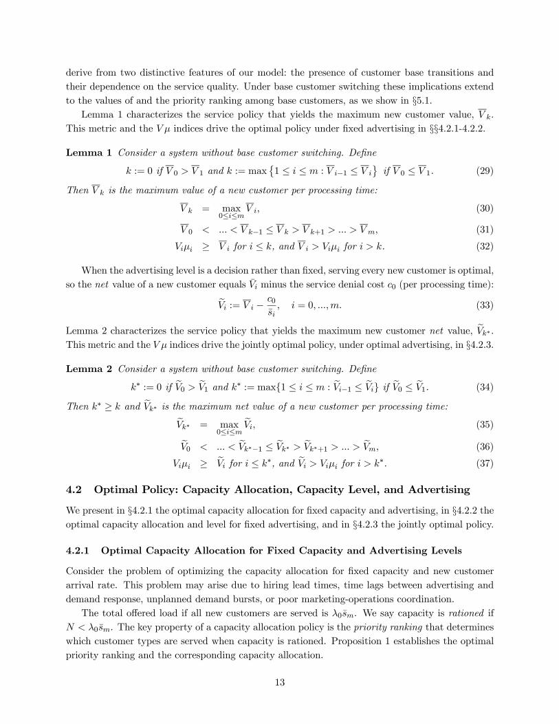
Example 1: Effect of Service-Independent Profit on Optimal Service Policy. Consider
the case where the service-independent profit of type 1 exceeds that of type 2: We fix 11 = 1000
and vary 22 ∈ [0 1000]. We assume equally loyal base customers: 11 = 22 = 03. Leaving
capacity cost aside, Figure 2(a) shows how the service-independent type-2 profit 22 effects a
new customer’s total value per processing time under three policies, serving no base customers
(e0), only those of type 1 (e1), or both types (e2), respectively. The policy that maximizes thisnew customer value denies service to type-2 customers (so ∗ = 1) if their service-independent
profit is below a threshold (22 820), but serves them otherwise (∗ = 2 for 22 ≥ 820).
19
Figure 2: Example 1: (a) New customer value per processing time as function of service policy and
service-independent type-2 profit 22. (b) Optimal policy as function of capacity cost and 22.
(11= 1000.)
By Proposition 3 the optimal service policy depends not only on the maximum new customer valuee∗ , but also on the index of lower ranked types ∗, and on the capacity cost . Figure 2(b)identifies the optimal policy depending on the capacity cost and the service-independent type-2
profit 22: By Proposition 3, it is not profitable to operate if the capacity cost exceeds ∗ ; it
is optimal to deny service to type-2 customers if ∗ = 1 and e1 22, which holds if their
service-independent profit is sufficiently low (22 820), but to serve all customers otherwise.
Example 2: Effect of Loyalty on Optimal Service Policy. Consider the case where type 1
are less loyal than type 2 after service denial: We fix 11 = 03 and vary 22 ∈ [03 10]. We assumeequally lucrative base customers: 1 = 2 = 800. As shown in Figure 3(a), leaving capacity cost
aside, the policy that maximizes a new customer’s total value per processing time serves all requests
only if type-2 customers’ loyalty is below a threshold (∗ = 2 for 22 ≤ 066), but denies service totype 2 if their loyalty is moderate (∗ = 1 for 066 22 ≤ 083) and to all base customers if type-2are very loyal upon service denial (∗ = 0 for 22 083). Figure 3(b) indicates the optimal servicepolicy depending on the capacity cost and the type-2 loyalty probability 22: By Proposition 3,
determining the optimal service policy requires comparing the capacity cost with 22 if ∗ = 1,
but with both 11 and 22 if ∗ = 0. These comparisons yield the four policies in Figure 3(b).
6.2 Using the Capacity Allocation Policy to Control the Customer Base
Our analysis implies that the capacity allocation policy plays a key role in controlling both the
composition and the size of the customer base: By targeting different service levels to different
customer types, the allocation policy can influence both the switching rates among, and the reten-
tion rates of, base customer types. Here we focus on the retention effects in the absence of base
customer switching. From (7) the ratio of customer bases of two types, say 1 and 2, satisfies
1
2=
0001(1 + 1(1− 111 − (1− 1) 11))
0002(2 + 2(1− 222 − (1− 2) 22)) (59)
20

Figure 3: Example 2: (a) New customer value per processing time as function of service policy and type-2
loyalty probability 22. (b) Optimal policy as function of capacity cost and 22. (11= 03).
where 000 is the type- joining rate and 1( + (1− − (1− ) )) the type- lifetime.
To illustrate how the optimal policy can effect this ratio we revisit Examples 1 and 2 of §6.1,
assuming both types have equal service-independent attrition rates (1 = 2). Recalling that both
types have equal probabilities for joining (01 = 02 = 02) and remaining (11 = 22 = 1) in the
customer base after being served, and equal normalized service request rates (11 = 22 = 10),
we have from (59) that, if giving equal service to both types is optimal (so ∗1 = ∗2), then theircustomer bases are equal, that is, ∗1 = ∗2. However, if serving only type 1 is optimal (so
∗1 = 1,
∗2 = 0) then the customer base of type 1 is larger than that of type 2: By (59) we have
∗1∗2=
2 + 2(1− 22)
1= 1 + 10(1− 22) (60)
where the fraction represents the ratio of type-2 to type-1 departure rates, and the second equality
holds since 1 = 2 and 22 = 10. The type-2 customer base is smaller because its members
leave at a larger rate due to service denial, at rate 2(1− 22) where 2 is their service request rate
and 22 is their loyalty probability given service denial. In Example 1, this probability is fixed at
22 = 03, so from (60) the type-2 departure rate is 81 and ∗1 = 8
∗2 whenever it is optimal to deny
service to type 2. However, in Example 2 the type-2 loyalty probability 22 varies, so the customer
base ratio ∗1∗2 depends not only on the optimal policy but also on this loyalty probability. To
illustrate this point, consider in Figure 3(b) how the optimal policy at a capacity cost of = 50
varies with 22. For 22 ≤ 075 it is optimal to serve all customers so that ∗1 = ∗2. For largervalues of 22 the optimal policy is to deny service to type-2 customers, but by (60) the customer
base ratio ∗1∗2 decreases in 22: the higher the loyalty of type-2 customers after service denial,
the larger their base relative to that of type-1. In the limit as 22 → 1, type-2 customers are so
loyal that they leave only for service-independent reasons, and we again have ∗1 = ∗2.
21
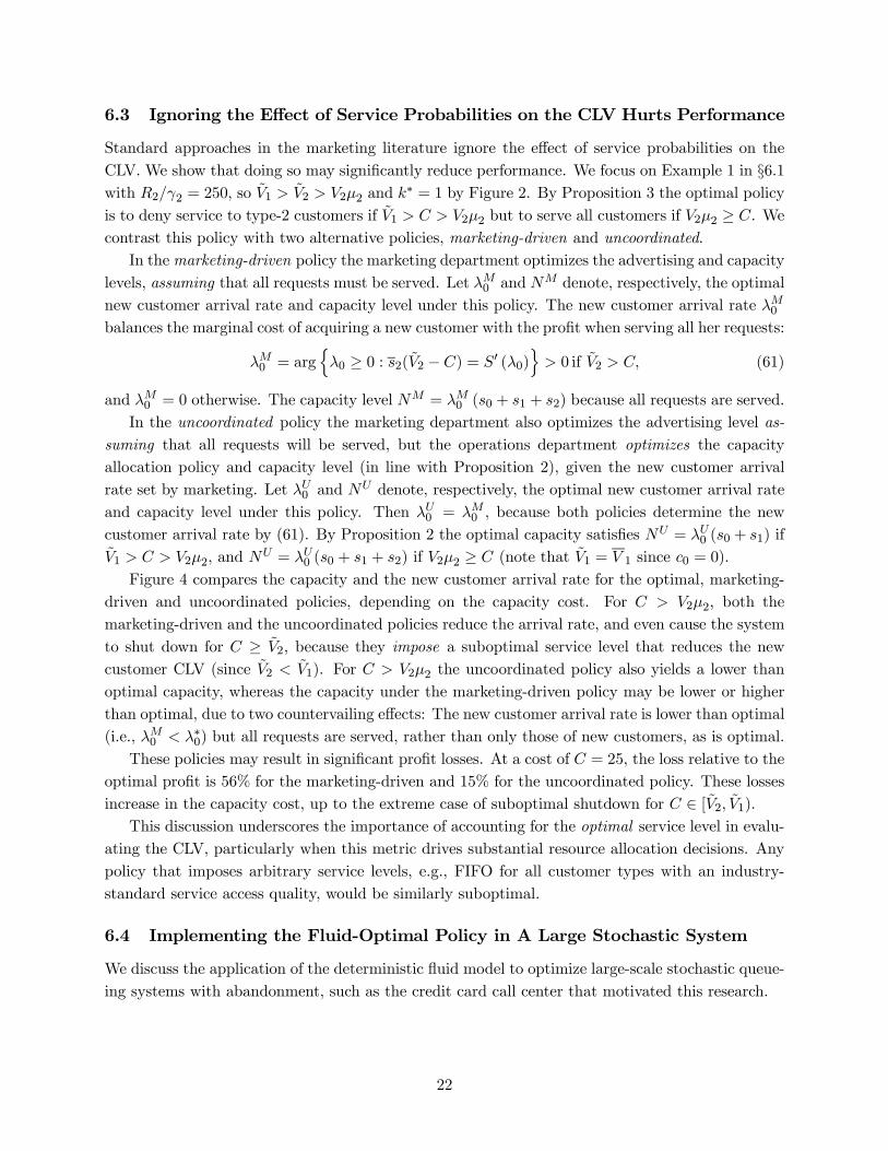
6.3 Ignoring the Effect of Service Probabilities on the CLV Hurts Performance
Standard approaches in the marketing literature ignore the effect of service probabilities on the
CLV. We show that doing so may significantly reduce performance. We focus on Example 1 in §6.1
with 22 = 250, so 1 2 22 and ∗ = 1 by Figure 2. By Proposition 3 the optimal policy
is to deny service to type-2 customers if 1 22 but to serve all customers if 22 ≥ . We
contrast this policy with two alternative policies, marketing-driven and uncoordinated.
In themarketing-driven policy the marketing department optimizes the advertising and capacity
levels, assuming that all requests must be served. Let 0 and denote, respectively, the optimal
new customer arrival rate and capacity level under this policy. The new customer arrival rate 0
balances the marginal cost of acquiring a new customer with the profit when serving all her requests:
0 = argn0 ≥ 0 : 2(2 − ) = 0 (0)
o 0 if 2 (61)
and 0 = 0 otherwise. The capacity level = 0 (0 + 1 + 2) because all requests are served.
In the uncoordinated policy the marketing department also optimizes the advertising level as-
suming that all requests will be served, but the operations department optimizes the capacity
allocation policy and capacity level (in line with Proposition 2), given the new customer arrival
rate set by marketing. Let 0 and denote, respectively, the optimal new customer arrival rate
and capacity level under this policy. Then 0 = 0 , because both policies determine the new
customer arrival rate by (61). By Proposition 2 the optimal capacity satisfies = 0 (0 + 1) if
1 22, and = 0 (0 + 1 + 2) if 22 ≥ (note that 1 = 1 since 0 = 0).
Figure 4 compares the capacity and the new customer arrival rate for the optimal, marketing-
driven and uncoordinated policies, depending on the capacity cost. For 22, both the
marketing-driven and the uncoordinated policies reduce the arrival rate, and even cause the system
to shut down for ≥ 2, because they impose a suboptimal service level that reduces the new
customer CLV (since 2 1). For 22 the uncoordinated policy also yields a lower than
optimal capacity, whereas the capacity under the marketing-driven policy may be lower or higher
than optimal, due to two countervailing effects: The new customer arrival rate is lower than optimal
(i.e., 0 ∗0) but all requests are served, rather than only those of new customers, as is optimal.These policies may result in significant profit losses. At a cost of = 25, the loss relative to the
optimal profit is 56% for the marketing-driven and 15% for the uncoordinated policy. These losses
increase in the capacity cost, up to the extreme case of suboptimal shutdown for ∈ [2 1).This discussion underscores the importance of accounting for the optimal service level in evalu-
ating the CLV, particularly when this metric drives substantial resource allocation decisions. Any
policy that imposes arbitrary service levels, e.g., FIFO for all customer types with an industry-
standard service access quality, would be similarly suboptimal.
6.4 Implementing the Fluid-Optimal Policy in A Large Stochastic System
We discuss the application of the deterministic fluid model to optimize large-scale stochastic queue-
ing systems with abandonment, such as the credit card call center that motivated this research.
22
Figure 4: Example 2 (22= 250): Capacity and new customer arrival rate as functions of the capacity
cost, for the optimal (∗), marketing-driven (), and uncoordinated () policies.
6.4.1 The Primitives of the Stochastic Queueing Model
Consider a service facility such as an inbound call center operating as a stochastic queueing system
with identical parallel servers. New customer arrivals are Poisson with rate 0. Type- base cus-
tomers’ call interarrival times, service times, and service-independent sojourn times are independent
draws from exponential distributions with means 1, 1 and 1, respectively. The financial
parameters (, and ) and the switching probabilities () are as in the deterministic model.
Unlike in the deterministic model, due to queueing delays and customer impatience the sto-
chastic system may fail to serve all requests even if it is underutilized. We model type- customers’
impatience by independent and exponentially distributed abandonment times with mean . Aban-
donments are equivalent to service denials (and denied requests are lost, as in the fluid model). In
this model customer base transitions depend on waiting times only through the resulting service
probabilities : conditional on the outcome of receiving or being denied service, a customer’s tran-
sition is independent of her waiting time. This assumption is consistent with the notions of “critical
incidents” and “end effects” in the service literature. The prevalent assumption is that customers
think about terminating their relationship with providers only when some critical incident occurs
(Keaveney 1995, Gremler 2004). In our setting the abandonment is the natural critical incident
— this is how customers signal that their waiting times are too long. Bitran et al. (2008a) (see
section 4.2.1 and references therein) suggest the presence of an “end effect”, whereby the outcome
of a service encounter may dominate the memory of the preceding waiting experience.
6.4.2 Implementing the Fluid-Optimal Policy in the Stochastic Queueing Model
Due to the state-dependence and feedback in customer flows, the relationships between the capacity
allocation policy and the service probabilities seem to be analytically intractable in the stochastic
model, unlike their counterparts (16) and (17) in the fluid model. It is therefore difficult to optimize
the stochastic system directly. However, simulation results summarized in §6.4.3 suggest that the
23
following natural implementation of the fluid-optimal capacity allocation policy yields near-optimal
performance for a stochastic system with sufficiently many servers: Operate a head-of-the-line
priority policy that gives customer types strict (nonpreemptive) priorities according to the ranking
specified in Part 1 of Proposition 1. (In the case with base customer switching the fluid-optimal
priority ranking is determined by solving the problem numerically.) This implementation assumes
flexible servers, so the firm can pool capacity across types. This is common in practice, including
in the credit card company discussed above. Another practice is to dedicate capacity to each type.
The fluid-optimal policy of Proposition 1 features two key differences to standard index policies
for systems with abandonment, such as the rule (Atar et al. 2010) and -type policies
(Tezcan and Dai 2010). (1) The indices consider the effect of service on customers’ future
requests and financial impact. (2) The values and e that determine the priority of one type— new customers — also depend on the indices of other types. These differences reflect that,
unlike standard models, ours captures customer base transitions that link future requests to past
service quality.
6.4.3 Summary of Simulation Results
We briefly summarize results from simulations (see Appendix B for details) that evaluate the
performance of the fluid-optimal policy in the stochastic queueing model described above. Focusing
for simplicity on the case of homogeneous base customers, we consider a number of customer
parameter combinations, some where it is never, and others where it may be, optimal to deny
service to base customers, according to Proposition 3. For each parameter combination we vary the
server cost in a range that yields enough servers, 100 or more, for the fluid model results to be
applicable. We compare (1) the fluid-optimal new customer arrival rate, capacity level, and priority
ranking with their counterparts from simulation-based optimization, and (2) the simulation-based
profit under the fluid-optimal prescriptions with the simulation-based optimal profit.
The main finding from over 350 simulation experiments is that on average the fluid-optimal
prescriptions yield a relative profit loss below 1%. We observe worse profit performance (losses
around 6%) only at capacity costs with jumps in the fluid-optimal service and capacity levels. (The
fluid-optimal new customer arrival rate and capacity typically deviate more from simulation-optimal
levels, whereas the fluid-optimal priority ranking is typically optimal for the stochastic system.)
7 Concluding Remarks
We study the profit-maximizing advertising, capacity, and capacity allocation policies for a service
firm with heterogeneous repeat customers whose acquisition, retention, and behavior during their
lifetime in the customer base depend on their service probability. We develop our results in the
context of a new fluid model that integrates CRM and capacity management. This model links the
makeup and value of the customer base both to the capacity allocation, unlike prior CRM models,
and to the service access quality of past interactions, unlike prior capacity management models.
We make several contributions to CRM and service capacity management: We derive new met-
rics that link the value of a customer to the capacity allocation policy and the resulting service
probabilities and customer base transitions of all types: the CLV of base customers, the index
24

and the policy-dependent value of a customer type. We provide new capacity management pre-
scriptions that hinge on these metrics, notably, optimality conditions for rationing capacity and
for identifying which customers to deny service. These results have important implications: Firms
need to understand how customer attributes affect the optimal policy; with repeat business the
capacity allocation policy plays a previously ignored key role in controlling the customer base;
marketing-focused policies that ignore the effect of service probabilities on the CLV may reduce
profits significantly; and the fluid model approach may also prove effective for CRM and capacity
management for stochastic systems such as the credit card call center that motivated this work.
Our results prescribe a ‘bang-bang’ structure for the optimal capacity allocation — customers
get either perfect service or none at all. This may seem unrealistic in some cases. However, it is
easy to modify these prescriptions to ensure a minimum, strictly positive, service probability even
for the least profitable types. The corresponding modified fluid-optimal capacity allocation can be
determined by adding minimum capacity constraints to the profit-maximization problem. Imple-
menting this modified allocation in a stochastic system would increase the fluid-optimal number of
servers and thereby reduce the delays and the abandonment rates of the lower-priority classes.
Our results also point to the interplay between the targeting levels of the advertising and
capacity allocation policies. On one hand, as shown in §6.3, imposing or assuming suboptimal
non-targeted service levels reduces the value of an acquired customer and yields lower than optimal
advertising spending. On the other hand, our results suggest that if the firm could better target
advertising and acquire more profitable customer types — our model assumes it cannot, then the
optimal service policy would target high service levels to more, or possibly all, customer types.
Our study focuses on a stationary environment that yields constant optimal arrival rates. In
non-stationary environments, for example, if the new customers’ demand response to advertising
changes over time, the optimal service probabilities may be time-dependent. Establishing the
structure of the optimal policies becomes more complicated as a result of the interplay between time-
dependent service probabilities and customer value metrics. However, if the capacity level can be
adjusted on the time scale of demand fluctuations, restricting attention to stationary service policies
while dynamically adjusting the advertising and capacity levels not only simplifies the analysis (the
customer value metrics presented in this paper remain valid) but may also be practically appealing
and near-optimal. Araghi (2014) studies a special case where the firm follows a periodic advertising
policy and the new customer arrival rate decays exponentially between advertising pulses.
We focus for simplicity on controlling the customer base through differentiated service levels
via the capacity allocation policy. However, our framework can be extended to allow for targeted
advertising to base customers. For example, in the case of the credit card company, base customers’
credit card spending, which corresponds to their service-independent profit , may depend both
on their service access quality and on advertisements. In this case the switching probabilities
would be functions of both the service probability and the advertising dollars targeted to type .
Finally, our model parameters can be estimated based on data that can be tracked. Such esti-
mates would help quantify the effects of service access quality attributes on CLV, a key requirement
for the practical implementation of capacity management policies that reflect CRM principles.
25

References
Adelman, D., A.J. Mersereau. 2013. Dynamic capacity allocation to customers who remember past
service.Management Sci. 59(3) 592—612.
Aflaki, S., I. Popescu. 2014. Managing retention in service relationships. Man. Sci. 60(2) 415—433.
Aksin, O.Z., M. Armony, V. Mehrotra. 2007. The modern call-center: a multi-disciplinary perspec-
tive on operations management research. Prod. & Oper. Management 16(6) 665-688.
Anand, K.S., M.F. Paç, S. Veeraraghavan. 2011. Quality—speed conundrum: trade-offs in customer-
intensive services. Management Sci. 57(1) 40-56.
Anderson, E.W., M. W. Sullivan. 1993. The antecedents and consequences of customer satisfaction
for firms. Marketing Sci. 12(2) 125—143.
Anton, J., T. Setting, C. Gunderson. 2004. Offshore company call centers: a concern to U.S.
consumers. Technical Report, Purdue University Center for Customer-Driven Quality.
Araghi M. 2014. Problems in service operations with heterogeneous customers. PhD Thesis, Uni-
versity of Toronto, Toronto, Canada.
Ascarza, E., B.G.S. Hardie. 2013. A joint model of usage and churn in contractual settings. Mar-
keting Sci. 32(4) 570—590.
Atar, R., C. Giat, N. Shimkin. 2010. The rule for many-server queues with abandonment.
Operations Research 58(5) 1427—1439.
Bitran, G.R., S. Mondschein. 1996. Mailing decisions in the catalog sales industry. Management
Sci. 42(9) 1364—1381.
Bitran, G.R., J. Ferrero, P. Rocha e Oliveira. 2008a. Managing customer experiences: perspectives
on the temporal aspects of service encounters.Manuf. Service Oper. Management 10(1) 61-83.
Bitran, G.R., P. Rocha e Oliveira, A. Schilkrut. 2008b. Managing customer relationships through
price and service quality. Working paper, IESE, Spain.
Blattberg, R. C., J. Deighton. 1996. Manage marketing by the customer equity test. Harvard Bus.
Rev. 74(4) 136—145.
Bolton, R.N. 1998. A dynamic model of the duration of the customer’s relationship with a contin-
uous service provider: the role of satisfaction. Marketing Sci. 17(1) 45-65.
Braun, M., D.A. Schweidel. 2011. Modeling customer lifetimes with multiple causes of churn. Mar-
keting Sci. 30(5) 881-902.
de Véricourt, F., Y.-P. Zhou. 2005. Managing response time in a call-routing problem with service
failure. Operations Research 53(6) 968—981.
Farzan. A., H. Wang, Y.-P. Zhou. 2012. Setting quality and speed in service industry with repeat
customers. Working paper, University of Washington.
26

Feichtinger, G., R. F. Hartl, S. P. Sethi. 1994. Dynamic optimal control models in advertising:
recent developments. Management Sci. 40(2) 195-226.
Feinberg, F.M. 2001. On continuous-time optimal advertising under S-shaped response. Manage-
ment Sci. 47(11) 1476—1487.
Gans, N. 2002. Customer loyalty and supplier quality competition.Management Sci. 48(2) 207-221.
Gans, N., Koole, G., Mandelbaum, A. 2003. Telephone call centers: tutorial, review and research
prospects. Manufacturing Service Oper. Management 5(2) 79—141.
Gaur, V., Y. Park. 2007. Asymmetric consumer learning and inventory competition. Management
Sci. 53(2) 227-240.
Genesys Telecommunications Labs. 2007. Genesys Global Consumer Survey. Daily City, CA, USA.
Green, L.V., P.J. Kolesar, W. Whitt. 2007. Coping with time-varying demand when setting staffing
requirements for a service system. Prod. & Oper. Management 16(1) 13—39.
Gremler. 2004. The critical incident technique in service research. J. Service Research 7(1) 65-89.
Günes, E. D., O. Z. Aksin, E. L. Örmeci, S. H. Özden. 2010. Modelling customer reactions to sales
attempts: if cross-selling backfires. J. Service Research 13(2) 168-183.
Gupta, S., D. Hanssens, B. Hardie, W. Kahn, V. Kumar, N. Lin, N. Ravishanker, S. Sriram. 2006.
Modeling customer lifetime value. J. Service Research 9(2) 139-155.
Hall, J., E. Porteus. 2000. Customer service competition in capacitated systems. Manufacturing
Service Oper. Management 2(2) 144-165.
Hanssens, D.M., L.J. Parsons, R.L. Schultz. 2001. Market response models: Econometric and time
series analysis. Springer.
Hassin R. 2016. Rational Queueing. Taylor & Francis, Boca Raton, FL.
Hassin R., M. Haviv. 2003. To Queue or not to queue: Equilibrium behavior in queueing systems.
Kluwer, Boston.
Ho, T.H., Y.H. Park, Y.P. Zhou. 2006. Incorporating satisfaction into customer value analysis:
Optimal investment in lifetime value. Marketing Sci. 25(3) 260-277.
Hopp, W.J., S. M. R.Iravani, G. Y. Yuen. 2007. Operations systems with discretionary task com-
pletion. Man. Sci. 53(1) 61-77.
Keaveney, M.S. 1995. Customer switching behavior in service Industries: an exploratory study. J.
Marketing 59(2) 71-82.
Lewis, M. A. 2005. Dynamic programming approach to customer relationship pricing. Management
Sci. 51(6) 986—994.
Liu, L., W. Shang, S. Wu. 2007. Dynamic competitive newsvendors with service-sensitive demands.
Manufacturing Service Oper. Management 9(1) 84-93.
27

Li, S., B. Sun, R.T. Wilcox. 2005. Cross-selling sequentially ordered products: an application to
consumer banking. J. Marketing Research 42(May) 233—239.
Musalem, A., Y.V. Joshi. 2009. How much should you invest in each customer relationship? A
competitive strategic approach. Marketing Sci. 28(3) 555-565.
Olsen, T.L., R.P. Parker. 2008. Inventory management under market size dynamics. Management
Science 54(10) 1805-1821.
Ovchinnikov, A., B. Boulu-Reshef, P.E. Pfeifer. 2014. Balancing acquisition and retention spending
for firms with limited capacity. Management Sci. 60(8) 2002-2019.
Pfeifer, P.E., A. Ovchinnikov. 2011. A note on willingness to spend and customer lifetime value for
firms with limited capacity. J. Interactive Marketing 25(3) 178-189.
Reinartz, W., J.S. Thomas, V. Kumar. 2005. Balancing acquisition and retention resources to
maximize customer profitability. J. Marketing 69(1) 63—79.
Reinartz, W., R. Venkatesan. 2008. Decision models for customer relationship management (CRM).
Wierenga B. (ed.) Handbook of Marketing Decision Models. Springer Science.
Rust, R.T., T.S. Chung. 2006. Marketing models of service and relationships. Marketing Sci. 25(6)
560-580.
Rust, R.T., A.J. Zahorik, T.L. Keinigham. 1995. Return on quality (ROQ): making service quality
financially accountable. J. Marketing 59(2) 58-70.
Rust, R.T., K. Lemon, V. Zeithaml. 2004. Return on marketing: using customer equity to focus
marketing strategy. J. Marketing 68(1) 109-127.
Rust, R. T., P. C. Verhoef. 2005. Optimizing the marketing interventions mix in intermediate-term
CRM. Marketing Sci. 24(3) 477—489.
Sasieni, M.W. 1971. Optimal advertising expenditure. Management Sci. 18(4) 64-72.
Schwartz, B. L. 1966. A new approach to stockout penalties. Management Sci. 12(12) B538—B544.
Sethi, S.P., Q. Zhang. 1995. Multilevel hierarchical decision making in stochastic marketing-
production systems. SIAM J. Control. and Optimization 33(2) 528-553.
Simon, J.L., J. Arndt. 1980. The shape of the advertising response function. Adv. Res. 20(4) 11-28.
Sun, B., S. Li. 2011. Learning and acting on customer information: a simulation-based demonstra-
tion on service allocations with offshore centers. J. Marketing Research 48(1) 72-86.
Tezcan, T., J. Dai. 2010. Dynamic control of N-systems with many servers: asymptotic optimality
of a static priority policy in heavy traffic. Operations Research 58(1) 94—110.
Venkatesan, R., V. Kumar. 2004. A customer lifetime value framework for customer selection and
resource allocation strategy. J. Marketing 68(4) 106 - 125.
28

Verhoef, P.C. 2003. Understanding the effect of CRM efforts on customer retention and customer
share development. J. Marketing 67(4) 30 - 45.
Yankee Group. 2006. Great expectations: self-service success can happen. Report, Yankee Group,
Boston. http://www.ccng.com/files/public/Yankee_SelfService.pdf.
Zeithaml, V. A., L.L. Berry, A. Parasuraman. 1996. The behavioral consequences of service quality.
J. Marketing 60 (4) 31—46.
29

Appendix A: Derivations and Proofs
Derivation of (15). It follows from the definition of (0) in (45) that
(e)− (0)
(e)= + +
X=1
(e)− (0)
(e)( − ) (62)
From (4) we have for T (e)−1 in terms of T (0)−1 and the outer product e
¡1 − 1 −
¢:
T (e)−1 = T (0)−1 − e
¡1 − 1 −
¢. (63)
Applying the Sherman—Morrison formula to (63), one can show that
(e) = (0) + (0)
P=1
¡ −
¢ (0)
1−P=1
¡ −
¢ (0)
(64)
Substituting (64) in (62) yields
(e)− (0)
(e)= ++
X=1
X=1
¡ −
¢ (0) ( − ) = ++
X=1
¡ −
¢ (0) =
Derivation of (18) and (47). Rearranging terms in (3) we get
00θ0 + xDDq(Θ−Θ)) = x (D +Dr (I−Θ)) (65)
Substituting D +Dr (I−Θ) = T (0)−1 from (4), it follows that the customer base vector satisfies
x =¡00θ0 + xDDq(Θ−Θ))
¢T (0) (66)
Equation (47) follows from (66), by substituting 00 = 00 from (16), and = for
≥ 1 from (17). Then, equation (18) for systems without base customer switching follows by
setting = = 0 for 6= ∈ {1 }.
Derivation of (19) and (48). Substitute 00 = 00 from (16), and = for ≥ 1from (17) into the profit function (8) to get:
Π=00 (0 + 0) +
X=1
( + ) +
X=1
( − )− 00 − − (0) (67)
If follows from (47) and the definition of (0) in (45) that
X=1
( − ) =
X=1
Ã000 +
X=1
¡ −
¢! (0) (68)
The total customer value (48) follows by substituting (68) and from (46) in (67). Then (48) also
agrees with (19) if = = 0 for 6= ∈ {1 }
1

Derivation of (50). From (10), (17), and (47) we can get
≤X=1
⎛⎝000 +
X=1 6=
¡ −
¢⎞⎠ (0)
1−P=1
¡ −
¢ (0)
(69)
Applying the Sherman—Morrison formula to (63) yields
(e) = (0)
1−P=1
¡ −
¢ (0)
(70)
Equation (50) follows from substituting (70) and from (49) in (69).
Derivation of (52). Let (C) be the total value generated, and (C) be the total capacityallocated, respectively, by allocating 0 to new customers and serving all base customer types in
C. By (48) and (51):
(C) = 00 (0 − 0) +X∈C
= 00
⎛⎝0 − 0 +X∈C
⎛⎝0 +X
∈C\{} (C)
⎞⎠
⎞⎠
(C) = 0 +X∈C
= 00
⎛⎝ 1
0+X∈C
⎛⎝0 +X
∈C\{} (C)
⎞⎠⎞⎠
Equation (52) follows from e (C) := (C) (C).
Derivation of (53). Let C be set obtained by adding type to C. Then the normalizedmarginal value and the normalized marginal capacity as we add type to C equals equal
¡C¢− (C)
00=X∈C
⎛⎝ X∈C\{}
³
³C´− (C)
´
⎞⎠ +
⎛⎝0 +X∈C
³C´
⎞⎠
¡C¢− (C)
00=X∈C
⎛⎝ X∈C\{}
³
³C´− (C)
´
⎞⎠+⎛⎝0 +
X∈C
³C´
⎞⎠
Now let I− denote the set all base customer types except . Equation (53) follows from
∆ (I I−) = (I)− (I−) (I)− (I−) =
P∈I−
P
∈I−
¡ (I)− (I−)
¢ + (0 +
P∈I−
(I) )P∈I−
P∈I−
¡ (I)− (I−)
¢ +
³0 +
P∈I− (I)
´
Proof of Lemma 1. Clearly (31) implies (30). The properties (31) and (32) follow from two
facts. () From (28), is a convex combination of −1 and :
=−1 −1 +
−1 + = 1 2 (71)
2

so is smaller than −1, equal to −1, or larger than −1, for every such that −1 ,
−1 = , or −1 , respectively. () By assumption +1+1 for ≥ 1.¥
Proof of Lemma 2. The proof of (36)-(37) is identical to that of (31)-(32). By the definition
of ∗ in (34), the inequality ≤ ∗ is equivalent to e−1 ≤ e if ≥ 1. Using (33) we havee−1 ≤ e ⇔ −1 − ≤ 0
µ1
−1− 1
¶
which is satisfied because −1 − ≤ 0 by (31), 0 ≥ 0, and −1 0.¥
Proof of Proposition 1. Part 1. Prioritizing base customers in decreasing order of their index is equivalent to the capacity allocation constraints
00 =⇒ +1 = 0 = 1 − 1 (72)
That is, customers of type +1 are only served if all of type are served (constraint (24) is binding
for ). This is optimal because +1+1 for ≥ 1 and by inspection of (22) and (24)-(25).We next establish the optimal priority of new customers. Let Π (0) denote the maximum
profit under the policy that prioritizes base customers of type ∈ {1 } over new customers,
new customers over base customers of type , and base customers in decreasing order of their
index. This policy is equivalent to (72) and the following capacity allocation constraints. All
base customer requests of type ∈ {1 } are served, i.e., (24) is binding:
= 00 = 1 (73)
and if some new customers are not served (so (23) is slack), no requests of type are served:
0 00 =⇒ = 0 (74)
To complete the proof of Part 1 we show that Π (0) ≥ Π (0) for 6= . The profit
Π (0) is the maximum value of the objective function in (22) under a capacity allocation vector
N that satisfies (23)-(25) and (72)-(74). Using (26), (28), and (73) we get
X=0
= 00 and
X=0
= 00,
and substituting into (22) and (25), respectively, it is straightforward to verify that
Π (0) = min (0 ) +
X=+1
min¡0 ( − 0−1)+
¢ − 00 − − (0) (75)
It remains to show Π (0) ≥ Π (0) for 6= . We have
Π (0)−Π−1 (0) = min (0 ) −min (0−1 ) −1−min¡0 ( − 0−1)
+¢
Using (71) to substitute for , and noting that
min¡0 ( − 0−1)
+¢= min (0)−min (0−1 )
3

we have
³Π (0)−Π−1 (0)
´=¡ − −1
¢(min (0−1 )− −1min (0 ))
Note that ≥ −1 ⇔ ≥ −1 by (71) and min (0−1 )− −1min (0) ≥ 0, so
Π (0) ≥ Π−1 (0)⇔ ≥ −1
It follows from (31) in Lemma 1 that Π (0) ≥ Π (0) for 6= .
Part 2. The capacity allocation specified in (38) is implied by (72)-(74) for = .
Part 3. By Part 1 and (75), Π∗ (0) satisfies (39). Lemma 1 implies that Π∗ (0) is concave
in .¥
Proof of Proposition 2. The condition for profitable operation, and Parts 1-2 follow from
the profit function (39) and from (31)-(32) in Lemma (1): () if ≥ then Π∗(0) ≤ 0 for
≥ 0, and () if then Π∗(0) is strictly increasing for ∈ [0 0), nondecreasing for
∈ [0−1 0] and = +1 if and only if ≥ , and strictly decreasing for 0.
This establishes (40). It follows from the optimal priority rule and the capacity allocation (38) of
Proposition 1, that it is optimal to serve the customer types as claimed. Furthermore, because
+1+1 for ≥ 1, rationing is optimal, i.e., ∗ 0 if and only if .
Part 3. The profit rate (41) follows from (39), by using (40) to substitute for ∗ and by notingthat − 0 = e from (33).¥
Proof of Proposition 3. We first prove the condition for profitable operation, that is,
max0≥0Π∗ (0) 0 if and only if e∗ , where Π∗ (0) is given by (41) for . Note
that this condition for profitable operation is more restrictive than and less restrictive
than e, because e∗ ≤ from (30), (33) and (35), and e ≤ e∗ from Lemma 2.
Because Π∗00 (0) 0 00 (0) and Π∗ (0) = 0, the maximizer ∗0 is unique, with ∗0 = 0 if
Π∗0 (0) ≤ 0, and ∗0 = arg{0 ≥ 0 : Π∗0 (0) = 0} 0 if Π∗0 (0) 0. Because 0 (0) = 0, (41) implies
Π∗0 (0) = (e − ) +
X=+1
( − )+ (76)
Note that Π∗0 (0) strictly decreases in . Therefore, Π∗0 (0) 0 ⇔ e∗ holds if, and only if,Π∗0 (0) = 0 for = e∗ , which we show next. For = e∗ we have from (76) that
Π∗0 (0) = (e − ) +
∗X=+1
( − ) = ∗(e∗ − ) = 0,
where the first equality follows because ≤ ∗ (Lemma 2) and ≥ e∗ for 1 ≤ ≤ ∗
((36)-(37) in Lemma 2 and decreases in ), and the second equality from (28) and (33).
Parts 1-2 follow from Parts 1-2 of Proposition 2 because e∗ ≤ and e∗ ≤ for 1 ≤ ≤ ∗.Part 3 follows by noting that for e∗ , the analysis in Part 1 implies
Π∗0 (0) = ∗(e∗ − ) +
X=∗+1
( − )+ 0,
4

and noting that Π∗ (0) = 0Π∗0 (0)− (0) in light of (41) yields (43) and (44).¥
Proof of Proposition 4. For convenience we restate the problem with WOM as follows:
maxN≥0≥00≥0
Π (N 0) = 00 0 +1
1 1 − 00 − − (0) (77)
0 ≤ 0
µ0
1 + +1
1
1
1 +
¶ (78)
1 ≤ 001 (79)
0 +1 ≤ (80)
where the customer metrics
0 : = 0 + 0 (81)
1 : = 1 − 0
1101
(82)
adjust those in the basic model by accounting for the indirect effects of the capacity allocation
N on the abandonment cost through the effective new customer arrival rate. The profit rate (77)
follows from (55), (57), and (81)-(82). The constraint (78) follows from (56) and (57).
We proceed in five steps.
1. Corollary 1 specializes Proposition 3 to the case of homogeneous base customers.
2. Lemma 3 characterizes the optimal capacity allocation N∗ for fixed and 0.
3. Lemma 4 characterizes the jointly optimal N∗ and ∗ for fixed 0.
4. Lemma 5 characterizes the jointly optimal N∗, ∗ and ∗0 .5. We use Corollary 1 and Lemma 5 to prove the claims of Proposition 4.
We use of the following relationships among the customer value metrics.
1 =000 + 111
0 + 1=
00 0 + 1
1 1
0 + 1 (83)
1 () =
01+
e0 + 111
01+
+ 1=
01+
0 0 + 1
1 1
01+
+ 1 (84)
The first equalities in (83) and (84) hold by (28) and (58), respectively, the second equalities because
00 0 = 000 + 0 by (81), 1
1 1 = 111 − 0 by (82), and e0 = (0 − 0)0 by (33).
Corollary 1 Suppose = 1. Under the optimal advertising, capacity and capacity allocation
policies it is profitable to operate if, and only if, max(e0 e1) . In this case:
1. If e0 11, it is optimal to prioritize and serve only new customers, rationing capacity,
∗ = ∗0 = ∗00, and the optimal new customer arrival rate satisfies
∗0 = argn0 ≥ 0 : 0(0 − ) = 0 (0)
o 0 (85)
2. If 11 ≥ , it is optimal to serve all customers, ∗ = ∗01, and the optimal new customerarrival rate satisfies
∗0 = argn0 ≥ 0 : 1(1 − ) = 0 (0)
o 0 (86)
where 1(1 − ) = 0(0 − ) + 1 (11 −)
5

Proof. Apply Proposition 3 with = 1, for Part 1 using ∗ = 0 and 11, and for Part
2 using ∗ = 0 or ∗ = 1 and ≤ 11.¤
Lemma 3 Fix the new customer arrival rate 0 and the number of servers .
If 0 0
1 1 then it is optimal to prioritize new customers, the optimal capacity allocation is
∗0 = min
Ã
00
1 + + ( − 00
1 + )+
01+
01+
+ 1 00
! (87)
∗1 = min
Ã( − 00
1 + )+
1
01+
+ 1 01
! (88)
and the optimal profit rate is
Π∗(0)=−00− (0)− +
⎧⎪⎨⎪⎩
0 0 ≤ 001+
001+
0 0 + ( − 00
1+)
1 ()
001+
01
01 1 01 ≤
(89)
If 0 0 ≤
1 1 then it is optimal to prioritize base customers, the optimal capacity allocation is
∗ = min (01 )
1 = 0 1 (90)
and the optimal profit rate is
Π∗ (0) = min (01 ) 1 − 00 − − (0) (91)
Proof. If 0 0
1 1, it is clear from the profit function (77), and the convexity of the
feasible region (78)-(80), that the solution maximizes0. Therefore it is optimal to strictly prioritize
new customers. We establish N∗ in (87)-(88) for each of the possible capacity intervals:If ≤ 00 (1 + ), then (80) binds, so ∗
0 = and ∗1 = 0, which agrees with (87)-(88).
If 00 (1 + ) 01, then (78) and (80) are binding, which yields
∗0 =
00
1 + + ( − 00
1 + )
01+
01+
+ 1 (92)
∗1 = ( − 00
1 + )
1
01+
+ 1 (93)
If 01 ≤ , then (78)-(79) bind, so ∗0 = 00 and ∗
1 = 11. In this case there is enough
capacity to serve all requests, and the effective new customer arrival rate equals 0.
That the solutions for 00 (1 + ) agree with (87)-(88) follows because ∗0 in (92)
satisfies ∗0 00 and ∗
1 in (93) satisfies ∗1 01 if, and only if, 01.
The profit (89) follows by substitutingN∗ in (77), using (84) and (92)-(93) for 00 (1 + )
01, and (83) and ∗ = 0 for 01 ≤ .
Next consider 0 0 ≤
1 1. It is clear from the profit function (77) and because the feasible
region (78)-(80) is convex, that the solution maximizes 1, so it is optimal to strictly prioritize
base customers. That is, (79) is binding, so 1 = 010 and (78) simplifies to 0 ≤ 00, which
yields N∗ in (90). The profit (89) follows by substituting N∗ in (77), using (83).¤
6

Lemma 4 Fix the new customer arrival rate 0. Under the capacity allocation policy it is profitable
to operate if, and only if, max( 0 0 1). In this case:
1. If 0 0
1 (), it is optimal to prioritize and serve only new customers, rationing
capacity, ∗ = ∗0 = 00 (1 + ), and the optimal profit is
Π∗ (0) =0
1 +
¡0( 0 − )− 0
¢− (0) (94)
2. If 0 0
1 () ≥ , or if
1 () ≥
0 0 and 1 , it is optimal to serve all customers,
∗ = 01, and the optimal profit is
Π∗ (0) = 0¡1( 1 − )− 0
¢− (0) (95)
Proof. The results follow from Lemma 3 and the two possible rankings of 0 0 and
1 1:
If 0 0
1 1 then
0 0 1 =
00 0 + 1
1 1
0 + 1
01+
0 0 + 1
1 1
01+
+ 1=
1 ()
1 1 (96)
The first equality holds by (83), the second by (84). The inequalities follow from 0 0
1 1.
If 0 0 ≤
1 1 then it follows similarly that
0 0 ≤ 1 =
00 0 + 1
1 1
0 + 1≤ 0
1+
0 0 + 1
1 1
01+
+ 1=
1 () ≤
1 1 (97)
The condition for profitable operation,max≥0Π∗(0) 0 if and only if max( 0 0 1),
follows from (96)-(97) and the profit functions (89) for 0 0
1 1 and (91) for 0 0 ≤
1 1.
Part 1. If 0 0
1 () then
0 0 1 1, so by Lemma 3 it is optimal to prioritize
new customers and Π∗ (0) satisfies (89), which is maximized at ∗ = ∗
0 = 00 (1 + ).
Substituting into (89) yields (94), because 00 0 = 0 0 + 0 from (28), (81) and 00 = 1.
Part 2. If max( 0 0 1) but the conditions of Part 1 do not hold, then (96)-(97) imply
that either 0 0
1 () ≥ , or
1 () ≥
0 0 and 1 , and furthermore, Π∗(0) in
(89) or (91) is maximized at ∗ = 01: Serving all customers is optimal under either priority
policy. Substituting into (89) or (91) yields (95).¤
Lemma 5 Under the optimal advertising, capacity, and capacity allocation policies it is profitable
to operate if, and only if, max(e0 e1). In this case:1. If e0
1 (), it is optimal to prioritize and serve only new customers, rationing
capacity, ∗=∗0 =∗0 0 (1 + ), and the optimal new customer arrival rate satisfies
∗0 = arg
½0 ≥ 0 : 1
1 + 0(e0 − ) = 0 (0)
¾ 0 (98)
2. If e0 1 () ≥ , or if e0 ≤
1 () and e1, it is optimal to serve all customers,
∗ = ∗0 1, and the optimal new customer arrival rate satisfies
∗0 = argn0 ≥ 0 : 1(e1 − ) = 0 (0)
o 0 (99)
7
Proof. By Lemma 4, for fixed 0 it is profitable to operate if and only if max( 0 0 1),
in which case the profit function Π∗ (0) satisfies (94) or (95). From (33) it follows that 0( 0 −)−0 = 0(e0−) in (94) and 1( 1−)−0 = 1(e1−) in (95). Therefore, if ≥ max(e0 e1)then max0≥0Π
∗ (0) = 0, so it is not profitable to operate.Parts 1-2 cover the two possible cases for max(e0 e1). Note that e1 = (0e0+111)(0+
1) by (28) and (33), and 1 () by (84) are convex combinations of
e0 and 11, and 1 () puts
a lower weight on e0. Therefore one of the following rankings holds:e0 e1 1 () 11 (100)e0 ≤ e1 ≤ 1 () ≤ 11 (101)
Part 1. If e0 1 (), then because
0 0 ≥ e0 by (33) and (81), the conditions of Part
1 of Lemma 4 hold. Therefore, it is optimal to prioritize and serve only new customers, and
Π∗ (0) =0
1 + 0(e0 − )− (0)
from (94) and (33). Because Π∗00 (0) 0 00 (0) and Π∗ (0) = 0, the maximizer ∗0 is uniquely
defined as ∗0 = 0 if Π∗0 (0) ≤ 0 and ∗0 = arg {0 ≥ 0 : Π∗0 (0) = 0} 0 if Π∗0 (0) 0.
Noting that
Π∗0 (0) =1
1 + 0(e0 − )− 0 (0)
and 0 (0) = 0, it follows that Π∗0 (0) 0 and ∗0 satisfies (98).
Part 2. If max(e0 e1) but the conditions of Part 1 do not hold, then (100)-(101) implythat either e0
1 () ≥ , or e0 ≤
1 () and e1. Furthermore, the conditions of Part
2 of Lemma 4 hold: If e0 1 () ≥ then
0 0 1 () ≥ . If e0 ≤
1 () and e1
then min( 1 1 ()) because
e1 ≤ 1 by (33) and e1 ≤ 1 () by (101), so that either
0 0
1 () ≥ , or
1 () ≥
0 0 and 1 holds. By Part 2 of Lemma 4, it is optimal
to serve all customers, and we have from (95) and (33) that
Π∗ (0) = 01(e1 −)− (0)
Because 0 (0) = 0, we have Π∗0 (0) 0. By the same argument as in Part 1, ∗0 satisfies (99).¤
It remains to prove the claims of Proposition 4, which follow from Corollary 1 and Lemma 5.
If e0 11 does not hold, then (100)-(101) imply that Part 2 of Corollary 1 and Part 2 of
Lemma 5 apply, so the solution is the same with or without WOM. Suppose that e0 11.
Part 1. If 0 1 () 11, then Part 1 of Corollary 1 and Part 2 of Lemma 5 apply,
so ∗0 satisfies (85) and ∗0 satisfies (99). We have ∗0 ∗0 and Π∗ (∗0 ) Π
∗ (∗0), becauseΠ∗ (0) and Π∗ (0) are strictly concave and 11 implies the inequality in
Π∗0 (0) = 0(e0 − ) + 1(11 − )− 0 (0) 0(e0 −)− 0 (0) = Π∗0 (0)
Part 2. If 0 1 () 11, then Part 1 of Corollary 1 and Part 1 of Lemma 5 apply,
so ∗0 satisfies (85) and ∗0 satisfies (98). We have ∗0 ∗0 and Π∗ (∗0 ) Π
∗ (∗0), becauseΠ∗ (0) and Π∗ (0) are strictly concave and
Π∗0 (0) =1
1 + 0(e0 − )− 0 (0) 0(e0 −)− 0 (0) = Π∗0 (0) ¥
8

Appendix B: Simulation Experiments
We evaluate the performance of the fluid model results of §4.2 against simulation results for the
stochastic system described in §§6.4.1-6.4.2. We focus on homogeneous base customers. We discuss
one representative case where denying service to base customers may be optimal in B.1, one where
doing so is never optimal in B.2, and further cases to show the robustness of these results in B.3.
For the advertising cost function we use the commonly assumed power model (0) = 0 ,
where 0 is a scale factor and 1 is the inverse of the customers’ response elasticity to the
advertising level (cf. Hanssens et al. 2001). We let = 05, = 15.
We assume a 24x7 operation. One time unit equals one day. We initialize the size of the
customer base with the value suggested by the fluid model, run the simulation for 5,100,000 new
customer arrivals, and discard the first 100,000 arrivals in computing performance measures.
For the simulation-based optimization, we vary the new customer arrival rate 0 in the interval
[1000,250000], increasing the step size with 0: We set the step size to 25, 250, 500, 1000, and 2500,
respectively, in the arrival rate intervals [1000,10000], [10000,20000], [20000,40000], [40000,100000],
and [100000,250000]. For each value of 0, we vary the number of servers in unit increments.
The fluid model results are applicable only for medium to large call centers, with 100 servers
or more. We limit the study to this scale range: We vary the server cost, , in increments of 100,
from 500 to the smaller of 5000 and the largest for which Proposition 3 prescribes ∗ ≥ 100.B.1 Representative case 1: denying service to base customers may be optimal (e0
11). This case occurs when the policy that serves only new customers maximizes their total value
per processing time, i.e., ∗ = 0. Table 2 summarizes the parameter values for this case. From (12)the base customers’ CLV as a function of their service probability ranges from 1(0) = $33167 to
1(1) = $45000. From (13), (15), and (33), we have e0 = $10 950 and 11 = $2 367, respectively.The highest capacity cost considered is = $3 400, for a total of 30 experiments. Both in the fluid
Parameter Value
Service rate of customers (per day) 100
Mean abandonment time of customers (days) 001
Call arrival rate per base customer (per day) 1 001
Prob. new customer joins customer base after service 01 03
Prob. base customer remains in customer base after service, abandoning 11 11 1 09
Call-independent departure rate per base customer (per day) 1 0002
Call-independent profit rate per base customer (per day) 1 10
Profit per served call of new, base customers 0 1 10−10Cost per abandoned call of new, base customers 0 1 025 05
Advertising cost function parameters (power model) 05 15
Table 2: Parameter Values for Representative Case 1: Higher OTV for New Customers (e0 11)
model and in the simulation, prioritizing new customers is optimal. Figure 5 visualizes the fluid
model performance. Figure 5(a) shows that the error in the new customer arrival rate prescribed by
the fluid model is lower than 6%. The error in the number of servers prescribed by the fluid model
is also lower than 6%, except for ∈ [2300 2900] where the errors are significant — up to around60%. They arise in the neighborhood of the server cost where the fluid-optimal regime switches
serving to denying service to base customers. By Proposition 3, the fluid-optimal number of servers
1

∗ drops discontinuously in the server cost at = 11 = 2 367 (from 325 to 130), whereas
the simulation-optimal server number decreases gradually in this neighborhood. On average the
profit loss is 089%. Figure 5(b) shows that the profit loss peaks in the neighborhood of the cost
= 11. However, at 59% this profit loss is significantly smaller than the error in the number
of servers prescribed by the fluid model. Intuitively, whereas the fluid-optimal number of servers
is discontinuous in the server cost at = 11, the profit rate is continuous at this cost. Outside
the cost range [2300 2900], the profit loss is smaller than 15%.
Figure 5: Fluid Model vs. Simulation: Percentage Errors in Optimal Number of Servers and New Customer
Arrival Rate, and Percentage Profit Loss, as Functions of the Capacity Cost (Priority to New Customers).
B.2 Representative case 2: denying service to base customers is not optimal (e0 11). This case occurs when the policy that serves all customers maximizes the new customers’
total value per processing time, i.e., ∗ = 1. We set 1 = 03. All other parameters remain the
same as in Table 2. From (13), (15), and (33), e0 = $4 317 and 11 = $6 789. For this case the
highest capacity cost is = 3900, for a total of 35 experiments.
Consistent with Proposition 1, prioritizing base customers is optimal in the simulation. The
results are qualitatively similar to those for Case 1 (we omit the details due to space constraints):
The fluid model prescriptions yield a near-optimal profit rate, and the percentage profit loss — on
average 028%, is typically smaller than the error in the fluid-optimal number of servers and new
customer arrival rate. However, in contrast to Case 1, here the error of the fluid model prescriptions
and the profit loss do not peak in some intermediate range of , because the fluid model prescribes
a balanced system for the entire cost range, so the fluid-optimal capacity is continuous in .
B.3 Robustness of the Fluid Model Prescriptions. To further test the robustness of the
fluid model we simulate ten additional scenarios, to cover all the combinations of 01 ∈ {03 05},11 ∈ {03 09}, and 1 ∈ {05 1 15}. All other parameters remain as in Table 2. For each scenariowe consider on average approximately 31 capacity cost levels (ranging from three to 46 depending
on the scenario), for a total of 313 experiments. The results for these scenarios are consistent with
the ones reported in B.1 and B.2. On average the profit loss is 17% in one scenario, and well below
1% in all others. We further find that the percentage profit loss under the fluid model prescriptions
decreases in the call-independent base customer profit rate, 1.
2