Collaborative part-based tracking using salient local

predictors

Wassim Bouachira,∗, Guillaume-Alexandre Bilodeaua

aLITIV lab., Department of Computer and Software Engineering,Ecole Polytechnique de Montreal,

P.O. Box 6079, Station Centre-ville, Montreal(Quebec), Canada, H3C 3A7

Abstract

This work proposes a novel part-based method for visual object tracking.In our model, keypoints are considered as elementary predictors localizingthe target in a collaborative search strategy. While numerous methods havebeen proposed in the model-free tracking literature, finding the most relevantfeatures to track remains a challenging problem. To distinguish reliable fea-tures from outliers and bad predictors, we evaluate feature saliency compris-ing three factors: the persistence, the spatial consistency, and the predictive

power of a local feature. Saliency information is learned during tracking tobe exploited in several algorithm components: local prediction, global local-ization, model update, and scale change estimation. By encoding the objectstructure via the spatial layout of the most salient features, the proposedmethod is able to accomplish successful tracking in difficult real life situa-tions such as long-term occlusion, presence of distractors, and backgroundclutter. The proposed method shows its robustness on challenging publicvideo sequences, outperforming significantly recent state-of-the-art trackers.Our Salient Collaborating Features Tracker (SCFT) also demonstrated a highaccuracy even if a few local features are available.

Keywords: Part-based tracking, Feature saliency, keypoint, SIFT,keypoint layout.

∗Corresponding authorEmail addresses: wassim.bouachir@polymtl.ca (Wassim Bouachir),

gabilodeau@polymtl.ca (Guillaume-Alexandre Bilodeau)

Preprint submitted to Computer Vision and Image Understanding March 15, 2015

1. Introduction1

Visual object tracking is a fundamental problem in computer vision with2

a wide range of applications including automated video monitoring systems3

[1, 2], traffic monitoring [3, 4], human action recognition [5], robot perception4

[6], etc. While significant progress has been made in designing sophisticated5

appearance models and effective target search methods, model-free tracking6

remains a difficult problem receiving a great interest. With model-free track-7

ers, the only information available on the target appearance is the bounding8

box region in the first video frame. Tracking is thus a challenging task due9

to (1) the insufficient amount of information on object appearance, (2) the10

inaccuracy in distinguishing the target from the background, and (3) the11

target appearance change during tracking.12

In this paper, we present a novel part-based tracker handling the afore-13

mentioned difficulties, including the lack of information on object appearance14

and features. This work demonstrates that an efficient way to maximize15

the knowledge on object appearance is to evaluate the tracked features. To16

achieve robust tracking in unconstrained environments, our Salient Collabo-17

rating Features Tracker (SCFT) discovers the most salient local features in18

an online manner. Every tracked local feature is considered as an elementary19

predictor having an individual reliability in encoding an object structural20

constraint, and collaborating with other features to predict the target state.21

To assess the reliability of a given feature, we define feature saliency as com-22

prising three factors: persistence, spatial consistency, and predictive power.23

Thereby, the global target state prediction arises from the aggregation of all24

the local predictions considering individual feature saliency properties. Fur-25

thermore, the appearance change problem (which is a major issue causing26

drift [7]) is handled through a dynamic target model that continuously in-27

corporates new structural properties while removing non-persistent features.28

Generally, a tracking algorithm includes two main aspects: the target rep-29

resentation including the object characteristics, and the search strategy for30

object localization. The contributions of our work relate to both aspects. For31

target representation, our part-based model includes keypoint patches encod-32

ing object structural constraints with different levels of reliability. Part-based33

representations are proven to be robust to local appearance changes and par-34

tial occlusions [8, 9, 10]. Moreover, keypoint regions are more salient and35

stable than other types of patches (e.g. regular grid, random patches), in-36

creasing the distinctiveness of the appearance model [11, 12]. Regarding the37

2

search strategy, the target state estimation is carried out via local features38

collaboration. Every detected local feature casts a local prediction expressing39

a constraint on the target structure according to the spatial layout, saliency40

information, detection scale, and dominant orientation of the feature. In this41

manner, feature collaboration preserves the object structure while handling42

pose and scale change without requiring to analyze the relationship between43

keypoints like in [9], neither calculating homographies such as in most key-44

point matching works [13, 14, 15].45

More specifically, the main contributions of this paper are:46

1. A novel method for evaluating feature saliency to identify the most47

reliable features based on their persistence, spatial consistency, and48

predictive power ;49

2. The explicit exploitation of feature saliency information in several algo-50

rithmic steps: (1) local predictions, (2) feature collaboration for global51

localization, (3) scale change estimation, and (4) for local feature re-52

moval from the target model;53

3. A dynamic appearance model where persistent local features are stored54

in a pool, to encode both recent and old structural properties of the55

target.56

4. Extensive experimentation to evaluate the tracker performance against57

five recent state-of-the-art methods. The experimental work conducted58

on challenging videos shows the validity of the proposed tracker, out-59

performing the compared methods significantly.60

The rest of this paper is organized as follows. In the next section, we61

review related part-based tracking works. Algorithm steps are presented62

in details in section 3. Experimental results are provided and analyzed in63

section 4, and section 5 concludes the paper.64

2. Related works65

Among various visual tracking algorithms, part-based trackers have at-66

tracted a great interest during the last decade. This is mainly due to the67

robustness of part-based models in handling partial changes, and to the effi-68

ciency of prediction methods in finding the whole target region given a subset69

of object parts. The fragment-based tracker of Adam et al. [16] is one of the70

pioneering methods in this trend. In their tracker, target parts correspond71

to arbitrary patches voting for object positions and scales in a competitive72

3

manner. The object patches are extracted according to a regular grid, and73

thus are inappropriate for articulated objects and significant in-plane rota-74

tions. Further, Erdem et al. demonstrated that the winning patch might75

not always provide reliable predictions [17]. This issue is addressed in [17]76

by differentiating the object patches based on their reliability. Therefore,77

every patch contributes to the target state prediction according to its relia-78

bility, allowing to achieve a better accuracy. Many other methods have been79

proposed for locating the object through parts tracking. The authors in [18]80

track object parts separately and predict the target state as a combination of81

multiple measurements. This method identifies inconsistent measurements82

in order to eliminate the false ones in the integration process. The method83

in [19] represents the shape of an articulated object with a small number of84

rectangular regions, while the appearance is represented by the corresponding85

intensity histograms. Tracking is then performed by matching local intensity86

histograms and by adjusting the locations of the blocks. Note that these last87

two trackers present the disadvantage of requiring manual initialization of88

object parts.89

In [10], the appearance model includes a combination between holistic and90

local representations to increase the model distinctiveness. In this model, the91

spatial information of the object patches is encoded by a histogram repre-92

senting the object structure. Similarly, Jia et al. sample a set of overlapped93

patches on the tracked object [8]. Their tracker includes an occlusion han-94

dling module allowing to locate the object using only visible patches. Kwon95

et al. [20] also used a set of local patches, updated during tracking, for tar-96

get representation. The common shortcoming of the last three trackers is97

the model adaptation mechanism in which the dictionary is updated simply98

by adding new elements, without adapting existing items. Another approach99

for creating part-based representations is the superpixel over-segmentation100

[21, 22]. In [21], Wang et al. use a discriminative method evaluating super-101

pixels individually, in order to distinguish the target from the background102

and detect shape deformation and occlusion. Their tracker is limited to103

small displacements between consecutive frames, since over-segmentation is104

performed only for a region surrounding the target location in the last frame.105

Moreover, this method requires a training phase to learn superpixel features106

from the object and the background.107

One of the major concerns in part-based tracking is to select the most sig-108

nificant and informative components for the appearance model. An interest-109

ing approach for defining informative components consists in using keypoint110

4

regions. Local keypoint regions (e.g. SIFT [23] and BRISK [24]) are more111

efficient than other types of patches in encoding object structure, as they112

correspond to salient and stable regions invariably detectable under various113

perturbation factors [25, 12]. Based on this, Yang et al. model the target114

with a combination of random patches and keypoints [26]. Keypoints layout115

is used to encode the structure while random patches model other appear-116

ance properties via their LBP features and RGB histograms. The target is117

thus tracked by exploiting multiple object characteristics, but the structural118

model captures only recent properties, as the keypoint model contains only119

those detected on the last frame. In a later work, Guo et al. [14] used a set120

of keypoint manifolds organized as a graph to represent the target structure.121

Every manifold contains a set of synthetic keypoint descriptors simulating122

possible variations of the original feature under viewpoint and scale change.123

The target is found by detecting keypoints on the current frame and match-124

ing them with those of the manifold model. This tracker achieved stable125

tracking of dynamic objects, at the cost of calculating homographies with126

RANSAC, which may be inappropriate for non-planar objects as shown in127

[9].128

Generalized Hough Transform (GHT)-based approaches have been re-129

cently presented as an alternative to homography calculation methods. GHT130

was initially used in context tracking [27], where the target position is pre-131

dicted by analyzing the whole scene (context) and identifying features (not132

belonging to the target) that move in a way that is statistically related to133

the target’s motion. In later works, this technique has been applied to ob-134

ject features in order to reflect structural constraints of the target and cope135

with partial occlusion problems. Nebehay et al. [9] propose to combine votes136

of keypoints to predict the target center. Although every keypoint votes in137

an individual manner, the geometrical relationship is analyzed between each138

pair of keypoints in order to rotate and scale votes accordingly. Furthermore,139

the keypoint model is not adapted to object appearance changes, arising only140

from the first observation of the target. In [28], the authors used an adaptive141

feature reservoir updated online to learn keypoint properties during tracking.142

The tracker achieved robust tracking in situations of occlusion and against143

illumination and appearance changes. However, this method does not han-144

dle scale changes and suffers from sensitivity to large in-plane rotations. In145

this paper we propose a novel tracking algorithm that exploits the geometric146

constraints of salient local features in a way to handle perturbation factors147

related to the target movement (e.g. scale change, in-plane and out-of-plane148

5

rotations), as well as those originating from its environment (i.e. occlusion,149

background clutter, distractors).150

3. Proposed method151

3.1. Motivation and overview152

In our part-based model, object parts correspond to keypoint patches153

detected during tracking and stored in a feature pool. The pool is initialized154

with the features detected on the bounding box region defined in the first155

video frame, and updated dynamically by including and/or removing features156

to reflect appearance changes. Instead of detecting local features in a region157

with a fixed size around the target location (like in [21, 14]), we eliminate158

the restriction of small displacements by using particle filtering to reduce159

the search space as proposed in [28]. This allows us to avoid computing local160

features on the entire image by limiting their extraction to most likely regions161

based on the target color distribution.162

When performing target search on a given frame, features from the pool163

are matched with those detected on the reduced search space. Following164

the matching process, the geometrical constraints (of the matched features)165

are adapted to local scale and pose changes as explained in section 3.3.1.166

Then all the matched features collaborate in a voting-based method (section167

3.3.2), to achieve global localization (section 3.3.3) and estimate the global168

scale change (section 3.3.4). Thus, the global prediction result corresponds169

to the aggregation of individual votes (elementary predictions). This method170

preserves the object structure and handles pose and scale changes, without171

requiring homography calculations such as in [14], neither analyzing the ge-172

ometrical relationship between keypoints like in [9]. The figure 1 presents a173

visual summary of the main algorithm steps.174

In order to keep the most relevant elements in the feature pool and exploit175

appropriately the most reliable predictors, each tracking iteration is followed176

by a saliency evaluation step. Saliency evaluation is performed to identify177

reliable features and determine the weights of their predictions accordingly,178

while eliminating irrelevant features from the appearance model. Our idea179

is inspired by the democratic integration framework of Triesch and von der180

Malsburg, where several cues contribute to a joint result with different levels181

of reliability [29]. In their approach, the elements that are consistent with182

the global result are considered as reliable and are assigned a higher weight183

in the future. This strategy has been adopted in other object tracking works184

6

(a) (b) (c)

Figure 1: Visual illustration of the main algorithm steps when tracking apartly occluded face in a moderately crowded scene. (a): the search space isreduced by using a color-based particle filter, and keypoints are detected inthe limited region (green dots). (b): matching the detected keypoints withthe appearance model allows to identify those belonging to the target. (c):matched features vote for the target center.

to perform an adaptive integration of cues according to their reliability [17,185

30, 31]. In our tracking method, the reliability is defined by the feature186

saliency including three factors: feature persistence, spatial consistency, and187

predictive power.188

• The persistence value ω of a given feature is used to evaluate the degree189

of co-occurrence between the target and the keypoint, and to determine190

if the feature should be removed from the pool.191

• The spatial consistency matrix Σ reflects the motion correlation be-192

tween the feature and the target center in the local prediction function.193

• The predictive power ψ indicates the accuracy of the past local predic-194

tions by comparison to the past global predictions. This value is used195

to weight the contribution of a local feature in the global localization196

function.197

Note that both the spatial consistency and the predictive power are de-198

signed to assess the feature quality. On the other hand, the persistence value199

is related to the occurrence level, disregarding the usefulness of the feature.200

Figure 2 illustrates situations where non-salient features can be identified201

through saliency evaluation. Non-salient features may correspond to out-202

liers included erroneously to the object model in the initialization step or203

when updating it. Such a feature may originate from the background as seen204

7

(a) (b)

(c)

Figure 2: Typical situations showing that saliency evaluation allows identi-fying bad predictors. Red and green dots represent, respectively, the targetcenter and the tracked feature. Continuous arrows represent the featureprediction initialization, while dotted arrows show inconsistent votes after acertain number of frames.

in figure 2a or belong to an occluding object (figure 2b) causing incorrect205

prediction. Once a keypoint is considered as non-salient, the corresponding206

local prediction (vote) will not be significant in the voting space, and/or207

its contribution will be reduced in the global localization procedure. More-208

over the feature is likely to be removed from the pool as soon as it becomes209

non-persistent.210

It should be noted that inconsistent features belonging to the tracked211

object may remain in the object model if they co-occur frequently with the212

target. An example is illustrated in figure 2c. However, their local predictions213

hardly affect the overall localization, since their quality indicators (Σ and ψ)214

will be reduced. While bad predictors are penalized and/or removed from the215

model, target global localization is carried out via a collaboration mechanism,216

exploiting the local predictions of the most salient features. The proposed217

tracking algorithm is presented in figure 3 and detailed in the next sections.218

3.2. Part-based appearance model219

In our tracker, the target is represented by a set of keypoint patches220

stored in a feature pool P . The proposed method could use any type of221

8

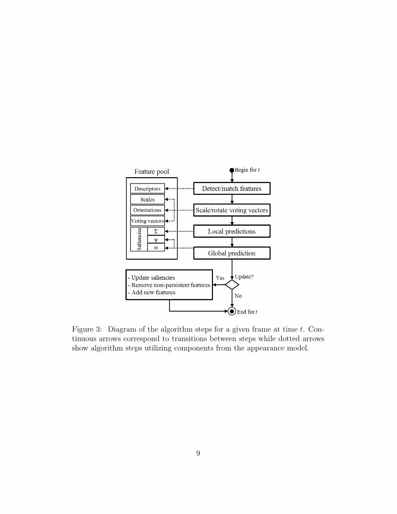
Figure 3: Diagram of the algorithm steps for a given frame at time t. Con-tinuous arrows correspond to transitions between steps while dotted arrowsshow algorithm steps utilizing components from the appearance model.

9

Figure 4: Adapting the voting vector to scale and orientation changes be-tween the first detection frame of the feature (left) and the current frame(right). The red and green dots represent, respectively, the target center andthe local feature.

scale/rotation invariant keypoint detector/descriptor. We used SIFT [23] as222

a keypoint detector/descriptor for its proven robustness [25]. We denote by223

f a feature from the pool P . All the detected features are then stored under224

the form225

f = [d, θ, σ, V, Sal], (1)

where:226

• d is the SIFT keypoint descriptor comprising 128 elements to describe227

the gradient information around the keypoint position;228

• θ is the detection angle corresponding to the main orientation of the229

keypoint;230

• σ is the detection scale of the keypoint;231

• V = [δx, δy] is a voting vector describing the target center location with232

respect to the keypoint location (see figure 4);233

• Sal = [ω,Σ, ψ] is the saliency information including persistence, spatial234

consistency, and predictive power indicators.235

Note that all the detection properties (i.e. d, θ, σ, and V ) are defined per-236

manently the first time the feature is detected, whereas saliency information237

(i.e. ω, Σ, and ψ) is updated every time features are evaluated.238

10

3.3. Global collaboration of local predictors239

In order to limit keypoint detection at time t to the most likely image area,240

we apply the search space reduction method that we previously proposed in241

[28]. Detected features from the reduced search space are then matched with242

those in the target model P in a nearest neighbor fashion. For matching a243

pair of features, we require that the ratio of the Euclidian distance from the244

closest neighbor to the distance of the second closest is less than an upper245

limit λ. The resulting subset Ft ⊆ P contains the matched target features246

at time t. After the matching process, the voting vectors (of the matched247

features) are adapted to local scale and pose changes as explained in the248

following.249

3.3.1. Voting vectors adaptation250

Each feature f ∈ Ft encodes a structural property expressed through its251

voting vector. Before applying the structural constraint of f , the correspond-252

ing voting vector V should be scaled and rotated according to the current253

detection scale σt and dominant orientation θt at time t as shown in figure 4.254

This adaptation process produces the current voting vector Vt = [δx,t, δy,t],255

with256

δx,t = ‖V ‖ρt cos(∆θ,t + sign(δy) arccosδx‖V ‖

), (2)257

δy,t = ‖V ‖ρt sin(∆θ,t + sign(δy) arccosδx‖V ‖

), (3)

where ∆θ,t and ρt are respectively the orientation angle difference and the258

scale ratio between the first and the current detection of f :259

∆θ,t = θt − θ, (4) ρt = σt/σ. (5)260

3.3.2. Local predictions261

After adapting the voting vectors to the last local changes, we base local262

predictions on GHT to build a local likelihood (or prediction) map Ml for263

every feature in Ft. For f , the local likelihood map is built in the reduced264

search space for all the potential object positions x using their relative posi-265

tions xf with respect to the keypoint location. The local likelihood map is266

defined using a 2D Gaussian probability density function as267

Ml(x) =1

√

2π|Σ|exp (−0.5 (xf − Vt)

>Σ−1(xf − Vt)). (6)

11

3.3.3. Global localization268

To achieve global prediction of the target position, features in Ft collabo-269

rate according to their saliency properties (persistence and predictive power).270

The global localization map Mg is thus created at time t to represent the271

target center likelihood considering all the detected features. Concretely, the272

global map is computed by aggregating local maps according to the equation273

Mg,t(x) =i

∑

f (i)∈Ft

ω(i)t ψ

(i)t M

(i)l,t (x). (7)

The final target location x∗t is then found as274

x∗t = argmax

x

Mg,t(x). (8)

3.3.4. Estimating the scale275

We also exploit saliency information to determine the target size St at276

time t. Scale change estimation is carried out by using the scale ratios of the277

most persistent keypoints. We denote by F∗t ⊂ Ft the subset including 50%278

of the elements in Ft, having the highest value of ωt. Then we compute279

St =1

|F∗t |

j∑

f (j)∈F∗

t

ρ(j)t S(j) (9)

to estimate the current target size, taking into account the object size S(j)280

when the jth feature was detected the first time.281

3.4. Model update282

The saliency information is updated with the object model when a good283

tracking is achieved. Our definition of a good tracking at time t is that the284

matching rate τt in the target region exceeds the minimum rate τmin. In this285

case saliency indicators are adapted and P is updated by adding/removing286

features.287

3.4.1. Persistence update288

If the matching rate τt shows a good tracking quality, the persistence289

value ω(i)t is updated for the next iteration with290

ω(i)t+1 = (1− β)ω

(i)t + β1{f (i)∈Ft}, (10)

12

where β is an adaptation factor and 1{f (i)∈Ft} is an indicator function defined291

on P to indicate if f (i) belongs to Ft. Following this update, we remove from292

P the elements having a persistence value lower than ωmin. On the other293

hand, the newly detected features (in the predicted target region) are added294

to P with an initial value ωinit.295

3.4.2. Spatial consistency296

The spatial consistency Σ is a 2x2 covariance matrix considered as a297

quality indicator and used in the local prediction function (Eq. 6). Σ is298

initialized to Σinit for a new feature. It is then updated to determine the299

spatial consistency between f (i) and the target center by applying300

Σ(i)t+1 = (1− β)Σ

(i)t + βΣ(i)

cur, (11)

where the current estimate of Σ is301

Σ(i)cur = (V (i)

cur − V(i)t )(V (i)

cur − V(i)t )>, (12)

and V(i)cur is the offset vector measured at time t given the global localization302

result. As a result, Σ decreases for consistent features, causing the votes to303

be more concentrated in the local prediction map. By contrast, the more304

this value increases during tracking (for inconsistent features), the more the305

votes become scattered.306

3.4.3. Predictive power307

In this step, we evaluate the predictive power of every keypoint contribut-308

ing to the current localization, considering the maxima of local prediction309

maps, and the global maximum corresponding to the final target position.310

This process, that we call prediction back-evaluation, aims to assess how good311

local predictions are. The local prediction for the ith feature is defined as the312

position313

x(i)t = argmax

x

M(i)l,t (x). (13)

The predictive power ψ(i)t+1 of f (i) at time t + 1 depends on the distances314

between its past predictions and the corresponding global predictions. We315

calculate ψ(i)t+1 with the summation of a fuzzy membership function as316

ψ(i)t+1 =

t∑

k=1

exp(−(x

(i)k − x∗

k)2

εS2k

) 1{f (i)∈Fk}(14)

13

Algorithm 1 Tracking algorithm

1: - initialize P2: for all frames do3: - Apply feature detector4: - Match features to get Ft ⊆ P5: for all matched features (f (i) ∈ Ft) do6: - Scale/rotate V (i): (Eq. 2 & 3)

7: - Compute local likelihood map M(i)l,t (x): (Eq. 6)

8: - Find local prediction result x(i)t : (Eq. 13)

9: end for10: - Compute global likelihood map Mg,t(x): (Eq. 7)11: - Find global location x∗

t : (Eq. 8) {output for frame t}12: - Estimate target size St: (Eq. 9) {output for frame t}13: if (τt ≥ τmin) then14: - Update ωt+1: (Eq. 10)15: - Remove non-persistent features (i.e. ωt+1 ≤ ωmin)16: for all matched features (f (i) ∈ Ft) do

17: - update Σ(i)t+1 (Eq. 11) and ψ

(i)t+1 (Eq. 14)

18: end for19: - Add new features to P20: - Initialize V , ω, Σ, and ψ for new features21: end if22: end for

where ε is a constant set to 0.005. The predictive power ψ increases as long317

as the feature achieves good local predictions. Consequently, the feature is318

considered as a reliable predictor, and its contribution in the global localiza-319

tion function (Eq. 7) becomes more prominent. We note that both Σ and ψ320

are designed to evaluate the feature quality. However, the former affects local321

predictions while the latter weights its contribution in the global localization.322

The overall tracking algorithm steps are presented in Alg. 1.323

14

4. Experiments324

4.1. Experimental setup325

4.1.1. The compared trackers326

We evaluated our Salient Collaborating Features Tracker (SCFT) by327

a comparison to recent state-of-the-art algorithms. Among the compared328

trackers, four are part-based methods already discussed in section 2. These329

trackers are the SuperPixel Tracker (SPT) [21], the Sparsity-based Collabo-330

rative Model Tracker (SCMT) [10], the Adaptive Structural Tracker (AST)331

[8], and the Structure-Aware Tracker (SAT) [28]. The fifth one is the online332

Multiple Support Instance Tracker (MSIT) [32] using a holistic appearance333

model. The corresponding source codes are provided by the authors with334

several parameter combinations. In order to ensure a fair comparison, we335

tuned the parameters of their methods so that for every video sequence in336

our dataset, we always use the best parameter combination among the pro-337

posed ones.338

4.1.2. Dataset339

We evaluate the trackers on 20 challenging video sequences. Sixteen of340

them are from an object tracking benchmark commonly used by the commu-341

nity [33]. The four other sequences jp1, jp2, wdesk, and wbook were captured342

in our laboratory room using a Sony SNC-RZ50N camera. The area was clut-343

tered with desks, chairs, and technical video equipment in the background.344

The video frames are 320x240 pixels recorded at 15 fps. We manually created345

the corresponding ground truths for jp1, jp2, wdesk, and wbook with 608, 229,346

709, and 581 frames respectively 1. Figure 5 presents the first frame of each347

of the sequences. In order to better figure out the quantitative results of our348

tracker, we categorized the video sequences according to the main difficul-349

ties that may occur in each sequence. The categorization of the sequences350

according to seven main properties is presented in table 1. This allows us to351

construct subsets of videos in order to quantitatively evaluate the trackers in352

several situations. Note that one video sequence may present more than one353

difficulty.354

1Our sequences are available at http://www.polymtl.ca/litiv/en/vid/.

15

Figure 5: The annotated first frames of the video sequences used for exper-iments. From left to right, top to bottom: tiger1, tiger2, cliffbar, David ,girl, faceocc, jp1, jp2, wdesk, wbook, David2, car, matrix, soccer, deer, skiing,jumping, Dudek, Mhyang, boy.

16

video LTOcc Distr BClut OPR Illum CamMo ArtObj

David X X

girl X X

faceocc X X

tiger1 X X

tiger2 X X

cliffbar X

jp1 X

jp2 X

wdesk X

wbook X

David2 X

car X

matrix X X X

soccer X X X X X

deer X X

skiing X X

jumping X

Dudek X X

Mhyang X

boy X X

Table 1: Main difficulties characterizing the test sequences. LTocc: Long-Term Occlusion, Distr: presence of Distractors, BClut: Background Clutter,OPR: Out-of-Plane Rotation, Illum: Illumination change, CamMo: CameraMotion, ArtObj: Articulated Object.

4.1.3. Evaluation methodology355

Success rate and average location error. In order to summarize a356

tracker’s performance on a video sequence, we use the success rate and the357

average location error. The success rate is measured by calculating for each358

frame the Overlap Ratio OR = area(Pr∩Gr)area(Pr∪Gr)

, where Pr is the predicted target359

region and Gr is the ground truth target region. For a given frame, tracking360

is considered as a success if OR ≥ 0.5. The Center Location Error (CLE)361

for a given frame consists in the position error between the center of the362

tracking result and that of the ground truth. The tables 2 and 3 present363

respectively the success rates and the average center location errors for the364

compared methods.365

Precision plot. While the average location error is known to be useful366

to summarize performance by calculating the mean error over the whole367

video sequence, this metric may fail to correctly reflect the tracker behavior.368

For example, the average location error for a tracker that tracks an object369

accurately for almost all the sequence before losing it on the last frames could370

be substantially affected by large CLEs on the last few frames. To address371

this issue, we adopt the precision plot used in [34] and [35]. This graphic372

17

video SPT SCMT AST MSIT SAT SCFT

David 62.37 60.22 37.63 63.44 100 100girl 84.16 1.98 17.82 0.99 84.95 85.94

faceocc 5.62 100 25.84 80.90 99.55 99.89

tiger1 60.56 25.35 30.99 2.82 50.99 80.28tiger2 46.27 16.42 31.34 5.97 70.15 75.74cliffbar 51.52 24.24 69.70 7.58 60.30 77.27jp1 18.09 78.13 84.38 3.78 89.14 99.41jp2 39.30 55.02 55.02 16.59 93.80 97.03

wdesk 13.68 57.26 32.30 10.01 90.47 93.96wbook 98.80 100 99.83 8.95 99.86 99.90

David2 36.44 90.69 38.55 94.23 98.70 100car 99.33 87.33 92 57.33 99.33 100

matrix 3 6 1 2 52 52soccer 16 31.33 36 37.33 69.33 69.33deer 12.68 4.23 18.31 4.23 95.77 100skiing 58.33 10 15 1.67 58.33 96.67jumping 36.42 84.35 10.22 3.19 95.53 99.04Dudek 100 100 100 79 100 100Mhyang 85.67 77.67 94.67 100 100 100boy 99.33 99.33 97.33 30 92 99.67

average 51.38 55.48 49.40 30.50 85.01 91.31

Table 2: Percentage of correctly tracked frames (success rate) for SCFT andthe five other trackers. Bold red font indicates best results, blue italics fontindicates second best.

shows the percentage of frames (precision) where the predicted target center373

is within the given threshold distance from the ground truth center.374

Success plot. By analogy to the precision plot that shows percentages375

of frames corresponding to several threshold distances of the ground truth,376

the authors in [33] argue that using one success rate value at an overlap ratio377

of 0.5 may not be representative. As suggested in [33], we use the success378

plot showing the percentages of successful frames at the ORs varied from 0379

to 1.380

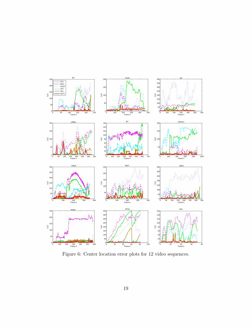
CLE and OR plots. Two other types of plots are used in our exper-381

iments to analyze in depth the compared methods : 1) the center location382

error versus the frame number presented in figure 6, and 2) the overlap ratio383

versus the frame number presented in figure 7. These plots are useful for384

monitoring and comparing the behaviors of several trackers over time for a385

given video sequence. We finally note that we averaged the results over five386

runs in all our experiments.387

18

0 50 100 150 200 2500

50

100

150

200

250

Frame #

CLE

jp2

ASTMSITSCMTSPTSATSCFT

0 100 200 300 400 5000

50

100

150

200

Frame #

CLE

David

0 100 200 300 400 500 6000

50

100

150

200

250

300

350

400

Frame #

CLE

girl

0 50 100 150 200 250 300 3500

50

100

150

200

Frame #

CLE

cliffbar

0 100 200 300 400 500 600 7000

20

40

60

80

100

120

140

160

Frame #

CLE

jp1

0 200 400 600 800 10000

50

100

150

200

Frame #

CLE

faceocc

0 200 400 600 8000

50

100

150

200

250

300

Frame #

CLE

wdesk

0 100 200 300 4000

50

100

150

200

250

Frame #

CLE

tiger1

0 50 100 150 200 250 300 3500

50

100

150

200

250

300

350

Frame #

CLE

tiger2

0 100 200 300 400 500 6000

50

100

150

200

250

Frame #

CLE

wbook

0 20 40 60 80 1000

50

100

150

200

250

300

350

400

Frame #

CLE

skiing

0 20 40 60 800

20

40

60

80

100

120

140

160

Frame #

CLE

deer

Figure 6: Center location error plots for 12 video sequences.

19

0 50 100 150 200 2500

0.2

0.4

0.6

0.8

1

Frame #

OR

jp2

ASTMSITSCMTSPTSATSCFT

0 100 200 300 400 5000

0.2

0.4

0.6

0.8

1

Frame #

OR

David

0 100 200 300 400 500 6000

0.2

0.4

0.6

0.8

1

Frame #

OR

girl

0 50 100 150 200 250 300 3500

0.2

0.4

0.6

0.8

1

Frame #

OR

cliffbar

0 100 200 300 400 500 600 7000

0.2

0.4

0.6

0.8

1

Frame #

OR

jp1

0 200 400 600 800 10000

0.2

0.4

0.6

0.8

1

Frame #

OR

faceocc

0 200 400 600 8000

0.2

0.4

0.6

0.8

1

Frame #

OR

wdesk

0 100 200 300 4000

0.2

0.4

0.6

0.8

1

Frame #

OR

tiger1

0 50 100 150 200 250 300 3500

0.2

0.4

0.6

0.8

1

Frame #

OR

tiger2

0 100 200 300 400 500 6000

0.2

0.4

0.6

0.8

1

Frame #

OR

wbook

0 20 40 60 80 1000

0.2

0.4

0.6

0.8

1

Frame #

OR

skiing

0 20 40 60 800

0.2

0.4

0.6

0.8

1

Frame #

OR

deer

Figure 7: Overlap ratio plots for 12 video sequences.

20

video SPT SCMT AST MSIT SAT SCFT

David 36.09 33.81 68.57 26.71 10.48 9.96girl 8.97 201.27 53.42 66.15 10.01 9.29

faceocc 116.84 5.07 85.43 23.36 14.26 5.58

tiger1 17.14 107.74 38.06 74.86 14.91 15.65

tiger2 22.81 189.50 29.15 44.58 16.13 10.25cliffbar 22.11 77.31 35.35 73.72 25.33 13.67jp1 35.21 17.74 16.66 97.08 7.03 4.75jp2 30.58 69.44 45.15 39.47 7.25 4.21

wdesk 79.92 34.17 80.97 122.62 11.12 14.31

wbook 11.27 5.09 8.68 131.57 11.87 5.91

David2 39.74 4.12 9.18 3.67 5.68 3.04car 6.65 6.98 4.92 34.67 6.16 4.51

matrix 43 79.87 57.74 74.82 26.23 26.23soccer 35.46 87.91 58.29 32.18 22.18 23.96

deer 39.66 56.79 54.58 96.52 7.42 5.39skiing 9.83 122.16 192.04 226.70 44.19 7.75jumping 22.01 7.41 90.03 55.75 11.21 8.15

dudek 6.11 4.28 4.74 15.08 9.92 8.14Mhyang 17.14 20.40 4.52 2.49 7.98 2.31boy 3.42 3.09 3.97 43.65 7.09 7.42

average 30.20 56.71 47.07 64.28 13.82 9.52

Table 3: Average location errors in pixels for SCFT and the five othertrackers. Bold red font indicates best results, blue italics font indicatessecond best.

4.2. Experimental result388

4.2.1. Overall performance389

The overall performance for several trackers is summarized by the average390

values in the tables 2 and 3 (last rows), as well as the average precision and391

success plots for the whole dataset (figure 8). All the metrics used for overall392

performance evaluation demonstrate that our proposed method outperforms393

all the other trackers, achieving an average success rate of 91.31% and an394

average localization error lower than 10 pixels. A major advantage of using395

success and precision plots is to allow choosing the appropriate tracker for a396

specific situation given the application requirements (e.g. high, medium, or397

low accuracy). In our experiments, the success and precision curves show the398

robustness of SCFT for all application requirements. SCFT is also the only399

tracker to reach 80% in precision for an error threshold of 15 pixels, and to400

produce a success rate exceeding 60% when the required OR is 80%. Except401

for SAT that realized the second best overall performance, and MSIT that402

had the last rank, the rankings of the other trackers are different depending403

on the considered metric. In the following subsections, the experimental404

results are discussed in details.405

21

0 0.2 0.4 0.6 0.8 10

0.1

0.2

0.3

0.4

0.5

0.6

0.7

0.8

0.9

1

Overlap threshold

Suc

ess

rate

Average success plots (whole dataset)

ASTMSITSCMTSPTSATSCFT

0 10 20 30 40 50 600

0.1

0.2

0.3

0.4

0.5

0.6

0.7

0.8

0.9

1

Location error threshold

Pre

cisi

on

Average precision plots (whole dataset)

Figure 8: Average success and average precision plots for all the sequences.

4.2.2. Long-term occlusion406

We evaluated the six methods in face tracking under long-term partial oc-407

clusion (up to 250 consecutive frames). In the faceocc and wbook, the tracked408

face remains partially occluded by an object several times for a long period.409

Some trackers drift away from the target to track the occluding object, which410

is mainly due to appearance model contamination by features belonging to411

the occluding object. Our method was able to track the faces successfully412

in almost all the frames under severe occlusion. The local predictions of a413

few detected features were sufficient for SCFT to achieve an accurate global414

prediction. Our target model may erroneously include features from the415

occluding object, but since we evaluate their motion consistency and predic-416

tive power, the corresponding local predictions will be scattered in the voting417

space and have small weights in the global localization function. The error418

plots for faceocc shows that SCMT and SAT also achieved good performances419

when the target was occluded (e.g. between frames 200 and 400). In fact,420

SCMT and SAT are also designed to handle occlusions, respectively through421

a scheme considering unoccluded patches, and a voting-based method that422

predicts the target center.423

In the wdesk sequence, the tracked face undergoes severe partial occlu-424

sions while moving behind a desk. SCFT, SAT and SCMT track the target425

correctly until frame #400 where the person performs large displacements426

causing SCMT to drift away from the face. Both SCFT and SAT continue427

the tracking successfully while the tracked person hides behind a desk, and428

our method achieved the best success rate of 93.96%.429

22

The success plots of long-term occlusion videos for SCFT and SAT show430

that both trackers can achieve more than 80% success rate as long as the431

required overlap ratio is lower than 0.5. Both trackers also had the two432

best precision curves, but SCFT performed significantly better under high433

requirement in accuracy (i.e. location error threshold lower than 15 pixels).434

As expected, the precision curve of MSIT is located below the others, since435

the holistic appearance model is not effective for a target undergoing severe436

occlusions.437

4.2.3. Presence of distractors438

The third and fourth rows of figure 10 present results of face tracking in439

moderately crowded scenes (four persons). In this experiments, our goal is440

to test the distinctiveness of the trackers. The success and precision plots441

for this category clearly show that SCFT and SAT are ranked respectively442

first and second regardless of the application requirements. This is mainly443

explained by the use of SIFT features that are proven to be effective in444

distinguishing a target face among a large number of other faces [36, 37, 38].445

In the jp1 video, we aim to track a face in presence of three other distract-446

ing faces, moving around the target and partially occluding it several times.447

The corresponding OR and CLE plots show that the proposed SCFTmethod448

produces the most stable tracking at the lowest error during almost all the449

608 video frames. Although the success rates of 89.14%, 84.38%, and 78.13%450

respectively for SAT, AST, and SCMT indicate good performances, the last451

two trackers drift twice (first at frame#530 and a second time at frame #570)452

to track distracting faces occluding or neighboring the target. We can also453

see in the OR and CLE plots that SAT drifts considerably three times, espe-454

cially between frames #341 and #397 when the tracked face region (person455

with a black t-shirt in the middle of the scene) is mostly occluded. However,456

neither the presence of similar objects near the target nor partial occlusion457

situations affected our SCFT tracker. The high performance of the proposed458

method in these situations is due to the distinctiveness of SIFT keypoints,459

in addition to the reliance on local predictions of the most salient features,460

even if outliers (from the background, neighboring or occluding faces) can be461

present in the feature pool.462

In the jp2 video, we track a walking person in the presence of four other463

randomly moving persons. The target crosses in front or behind distractors464

that may occlude it completely for a short period. All the five other methods465

confused the target with an occluding face, at least for a few frames after full466

23

0 0.2 0.4 0.6 0.8 10

0.1

0.2

0.3

0.4

0.5

0.6

0.7

0.8

0.9

1

Overlap threshold

Suc

ess

rate

Success plots for long−term occlusion videos

ASTMSITSCMTSPTSATSCFT

0 10 20 30 40 50 600

0.1

0.2

0.3

0.4

0.5

0.6

0.7

0.8

0.9

1

Location error threshold

Pre

cisi

on

Precision plots for long−term occlusion videos

0 0.2 0.4 0.6 0.8 10

0.1

0.2

0.3

0.4

0.5

0.6

0.7

0.8

0.9

1

Overlap threshold

Suc

ess

rate

Success plots for distractors videos

0 10 20 30 40 50 600

0.1

0.2

0.3

0.4

0.5

0.6

0.7

0.8

0.9

1

Location error threshold

Pre

cisi

onPrecision plots for distractors videos

0 0.2 0.4 0.6 0.8 10

0.1

0.2

0.3

0.4

0.5

0.6

0.7

0.8

0.9

1

Overlap threshold

Suc

ess

rate

Success plots for background clutter videos

0 10 20 30 40 50 600

0.1

0.2

0.3

0.4

0.5

0.6

0.7

0.8

0.9

1

Location error threshold

Pre

cisi

on

Precision plots for background clutter videos

Figure 9: Success and precision plots for long-term occlusion, distractors,and background clutter videos.

24

Figure 10: Tracking results for several trackers on the video sequences David,faceocc, jp1, jp2, and tiger1 (from top to bottom).

occlusion. Nevertheless, SCFT is able to recover tracking correctly as soon467

as a small part of the target becomes visible. For both distractors sequences468

jp1 and jp2, SCFT produced simultaneously the highest success rate and469

the lowest average error.470

4.2.4. Illumination change, camera motion471

The video sequence David is recorded using a moving camera, following472

a walking person. The scene illumination conditions change gradually as the473

person moves from a dark room to an illuminated area. The face also under-474

goes significant pose change during movement. All the trackers, except AST,475

were able to track the face successfully in more than 60% of the frames. Once476

again, SCFT achieved the best success rate and the lowest average error.477

This experiment shows the efficiency of our appearance model, allowing the478

25

tracker deal robustly with illumination variation. Our method is also not479

affected by large and continuous camera motion since features are detected480

wherever the space reduction method shows a significant likelihood of finding481

the target. On the other hand, in-plane rotations are handled efficiently in482

the global prediction function since we exploit the information on keypoint483

local orientation changes.484

4.2.5. Out-of-plane rotation485

The target person’s face in the girl video, exhibits pose change and out-of-486

plane rotations abruptly. SPT, SAT, and SCFT were able to track the face487

correctly in more than 80% of the frames. SCFT achieved the best success488

rate, handling efficiently pose change and partial occlusion. Our tracking489

was accurate as long as the girl’s face was at least partly visible. We lost the490

target when the face was turned away from the camera, but we were able to491

recover tracking quickly as soon as it partially reappeared.492

4.2.6. Background clutter, articulated object493

The main difficulty with the cliffbar, tiger1, and tiger2 videos is the clut-494

tered background whose the appearance may disrupt the tracker. For this495

category, the success and precision curves of SCFT are located above the496

others, showing the advantage of our method for all the tested thresholds of497

OR and CLE. Always based on the success and precision plots, we can see498

that SAT and SPT were ranked respectively second and third. It is note-499

worthy that both methods include discriminative aspects facilitating track-500

ing under such conditions. In fact, SPT uses a discriminative appearance501

model based on superpixel segmentation while SAT utilizes information on502

the background color distribution to evaluate the tracking quality.503

In the Cliffbar sequence, a book is used as a background having a sim-504

ilar texture to that of the target. SCFT outperformed significantly all the505

competing methods in both success rate and average location error. AST,506

SAT, and SPT also performed relatively well, taking into account the diffi-507

culty of the sequence. Indeed, the target undergoes abrupt in-plane rotations508

and drastic appearance change because of high motion blur. The proposed509

tracker is hardly affected by these difficulties since it continues adapting510

the appearance model by including/removing keypoints, and handling pose511

change through keypoint orientations.512

In the tiger1 and tiger2 sequences, the target exhibits fast movements513

in a cluttered background with frequent occlusions. Owing to partial pre-514

26

dictions that localize the target center using a few visible keypoints, SCFT515

had the highest percentages of correct tracks for both videos. SAT also516

overcomes the frequent occlusion problem via its voting mechanism that pre-517

dicts the target position from available features. The other methods fail to518

locate the stuffed animal, but SPT had relatively better results due to its dis-519

criminative model facilitating the distinction between target superpixels and520

background superpixels. Note that the tracked object in tiger1 and tiger2 is521

a deformable stuffed animal. The predictions of features located on articu-522

lated parts are consequently inconsistent with the overall consensus, but this523

issue is effeciently handled by the use of spatial consistency and predictive524

power that reflect the predictors’ reliability. These features may remain in525

P and continue predicting the target position without affecting the global526

result (because of low predictive power and spatial consistency). Our feature527

pool may also erroneously include outliers from the background, identified528

as non-persistent to be removed from the model.529

4.2.7. Sensitivity to the number of features530

One of the most challenging situations encountered in our dataset is the531

partial occlusion. The target faces in the faceocc, wdesk, and wbook videos532

undergo severe long-term occlusions causing the number of detected features533

to decrease drastically. Since local features detection represents a critical534

component for part-based trackers, we propose to study the impact of the535

number of features on SCFT’s performance. We considered the video se-536

quences faceocc, wdesk, and wbook, and analyzed the number of detected537

features on every video frame. We computed the average CLE value for each538

subset of frames having their numbers of collaborating features within the539

same interval (spanning 10 values). This allows us to create a scatter plot540

representing the average CLE versus the number of collaborating features541

(figure 11). To investigate the relationship between the number of features542

and the CLE, we model the plot by fitting a fourth degree predictor function543

and a linear function. The plot shows that the smallest numbers of features544

produce an average CLE not exceeding nine pixels. After that, the fitted545

fourth degree function decreases before stabilizing around the mean value of546

four pixels when more than 30 features are detected. Regarding the linear547

function (y = ax+ b), it is obvious to expect that the coefficient a would be548

negative since the CLE becomes lower when the number of features increases.549

However, a high absolute value for a would suggest that the algorithm re-550

quires a large number of features to achieve accurate tracking. In our case,551

27

0 50 100 150 200 250 300 3500

2

4

6

8

10

12

14

Number of collaborating features

aver

age

CLE

Scatter plot Linear fitting 4th degree fitting

Figure 11: Sensitivity of SCFT’s localization error (in pixels) to the numberof collaborating features (sequences faceocc, wdesk, and wbook). Data pointsfrom the scatter plot correspond to interval centers.

the linear coefficients estimation (a = −0.0064; b = 5.1107) demonstrate552

that the error barely increases when the number of collaborating features553

diminishes from the maximum (i.e. 345 features) to one feature. This as-554

certainment confirms that the collaboration of a few number of unoccluded555

features is sufficient for our tracker to ensure accurate tracking.556

4.2.8. Sensitivity to the saliency factors557

In this section, we analyze the effect of the saliency factors separately on558

the tracking performance. We created three versions of SCFT:559

• v-ω: the persistence indicator ω is not used in the global prediction560

function;561

• v-ψ: the predictive power ψ is completely removed from the algorithm;562

• v-Σ: the spatial consistency matrix is not updated, and is the same for563

all the features (Σ = Σinit).564

The tables 4 and 5 respectively present the percentages of correctly tracked565

frames and the average location errors for SCFT and the three other versions566

of the tracker on a subset of five video sequences. The selected sequences567

cover almost all the situations in table 1, and each video includes several568

28

video v-ω v-ψ v-Σ SCFT

girl 43.56 56.44 63.55 85.94tiger1 71.03 78.87 74.63 80.28David2 89.20 95.51 97.53 100deer 88.18 92.52 92.25 100boy 80.22 91.15 88.06 99.67

average 74.44 82.90 83.20 93.18

Table 4: Percentage of correctly tracked frames for four versions of the pro-posed tracker. v-ω: the tracker do not use persistence indicators to weightlocal predictions, v-ψ: the tracker does not evaluate the predictive power offeatures, v-Σ: the spatial consistency matrix is the same for all the features.Bold red font indicates best results, blue italics font indicates second best.

difficulties. The obtained results show that the tracking performance is more569

affected when the persistence indicator is not considered (version v-ω). In570

fact,, v-ψ and v-Σ outperformed v-ω for all the five sequences. This result571

can be explained by the fact that with the removal of one factor among572

ψ and Σ, the remaining one continues to take into account the precision573

of the feature’s past predictions, since both the spatial consistency and the574

predictive power are designed to assess the feature quality. However, if the575

indicator ω is not considered, the prediction step no longer takes into ac-576

count the occurence level of the keypoint. Furthermore, these experiments577

demonstrated the complementarity of the three saliency factors, as the best578

performance is obtained when the three indicators are evaluated and up-579

dated during tracking. We finally note that the saliency evaluation method580

proposed in this work can be adapted or applied directly to a wide range of581

tracking algorithms that are based on the voting of local features.582

4.2.9. Sensitivity to parameters583

Most of the parameters of our algorithm were set to default values for all584

the video sequences. In our experimental work, only three parameters were585

tuned to optimize the performance of the tracker:586

• N∗ : the number of particles defining the reduced search space, where587

keypoints are detected;588

• τmin : the minimum matching rate that is required to update the ap-589

pearance model;590

29

video v-ω v-ψ v-Σ SCFT

girl 17.98 14.49 13.24 9.29tiger1 17.02 16.89 16.98 15.65David2 8.06 6.36 5.11 3.04deer 10.19 8.13 7.63 5.39boy 11.16 7.98 7.51 7.42

average 12.88 10.77 10.09 8.16

Table 5: Average location errors in pixels for four versions of the proposedtracker. v-ω: the tracker does not use persistence indicators to weight localpredictions, v-ψ: the tracker does not evaluate the predictive power of fea-tures, v-Σ: the spatial consistency matrix is the same for all the features.Bold red font indicates best results, blue italics font indicates second best.

parameters girl tiger1 David2 deer boy

N∗ 30 100 100 20 50

τmin 0.55 0.8 0.3 0.2 0.2

ωmin 0.3 0.4 0.1 0.4 0.4

Table 6: Parameter values used in SCFT with each video from the subsetincluding girl, tiger1, David2, deer, and boy.

• ωmin : the persistence threshold used to determine if the feature should591

be removed from the model;592

In order to evaluate the sensitivity of SCFT to parameters, we considered593

the same subset of five sequences and ran our tracker multiple times on each594

video, using the optimized parameters of the other videos. The optimized595

parameter values for each video are shown in table 6.596

The results of these runs are reported in the tables 7 and 8, where the597

A.D. column shows the Average Difference between the result obtained with598

the optimized set of parameters and those obtained with the parameter sets599

of the four other sequences. As we can see, 13.33% is the most significant600

average decrease in sucess rate (for the girl video), while the highest average601

increase in localization error is that of the David2 sequence (4.3 pixels).602

On the other hand, parameter change had a very low impact on the video603

sequences deer (1.41% as average decrease in sucess rate) and boy (1.30 pixels604

as average increase in localization error). In general, SCFT was able to605

achieve a stable tracking for all the runs and the performance of our tracker606

30

girl tiger1 David2 deer boy A.D.

girl 85.94 81.19 75.26 72.58 61.41 13.33tiger1 76.06 80.28 70.42 80 80.28 3.59David2 94.60 88.45 100 94.04 95.53 6.84deer 97.18 100 97.18 100 100 1.41boy 95 93 90.67 98 99.67 5.50

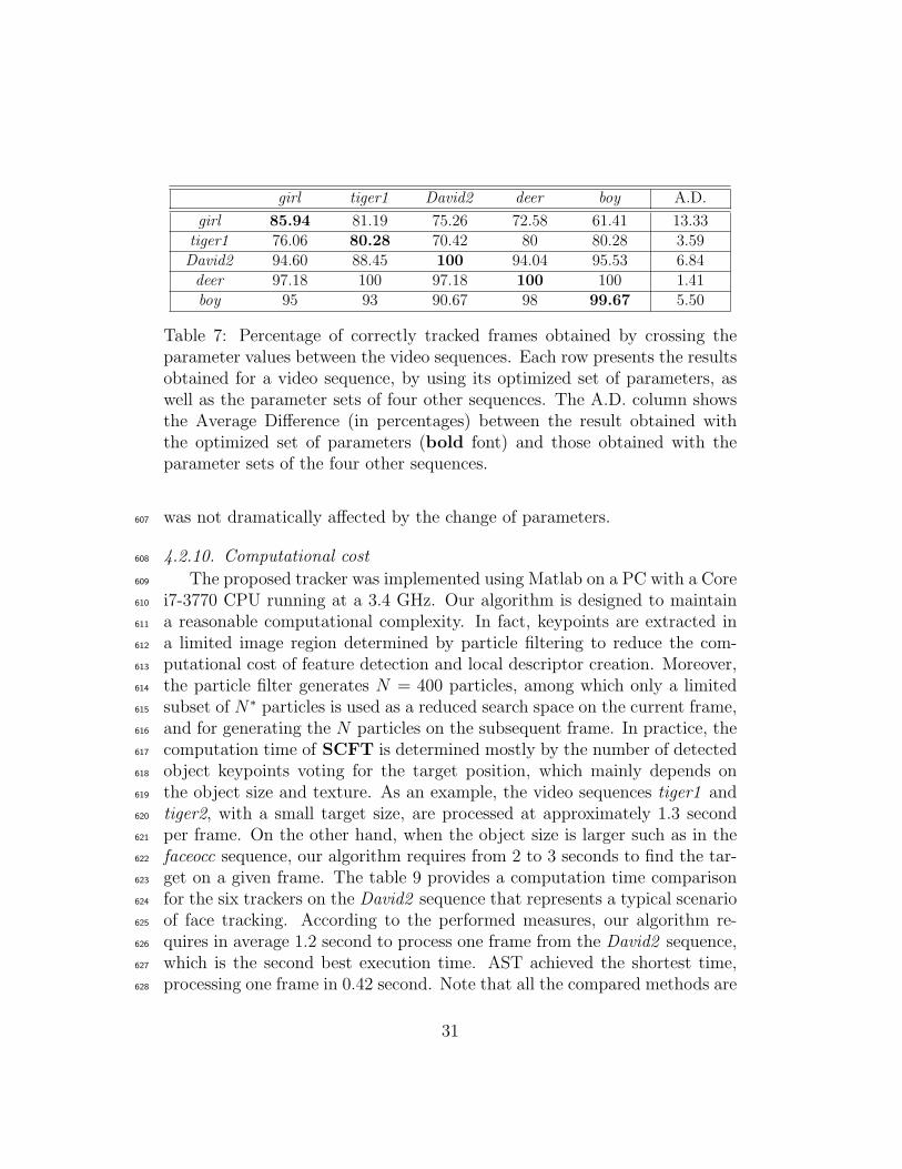
Table 7: Percentage of correctly tracked frames obtained by crossing theparameter values between the video sequences. Each row presents the resultsobtained for a video sequence, by using its optimized set of parameters, aswell as the parameter sets of four other sequences. The A.D. column showsthe Average Difference (in percentages) between the result obtained withthe optimized set of parameters (bold font) and those obtained with theparameter sets of the four other sequences.

was not dramatically affected by the change of parameters.607

4.2.10. Computational cost608

The proposed tracker was implemented using Matlab on a PC with a Core609

i7-3770 CPU running at a 3.4 GHz. Our algorithm is designed to maintain610

a reasonable computational complexity. In fact, keypoints are extracted in611

a limited image region determined by particle filtering to reduce the com-612

putational cost of feature detection and local descriptor creation. Moreover,613

the particle filter generates N = 400 particles, among which only a limited614

subset of N∗ particles is used as a reduced search space on the current frame,615

and for generating the N particles on the subsequent frame. In practice, the616

computation time of SCFT is determined mostly by the number of detected617

object keypoints voting for the target position, which mainly depends on618

the object size and texture. As an example, the video sequences tiger1 and619

tiger2, with a small target size, are processed at approximately 1.3 second620

per frame. On the other hand, when the object size is larger such as in the621

faceocc sequence, our algorithm requires from 2 to 3 seconds to find the tar-622

get on a given frame. The table 9 provides a computation time comparison623

for the six trackers on the David2 sequence that represents a typical scenario624

of face tracking. According to the performed measures, our algorithm re-625

quires in average 1.2 second to process one frame from the David2 sequence,626

which is the second best execution time. AST achieved the shortest time,627

processing one frame in 0.42 second. Note that all the compared methods are628

31

girl tiger1 David2 deer boy A.D.

girl 9.29 11.58 12.66 12.55 13.29 3.23tiger1 16.18 15.65 21.17 18.31 16.27 2.32David2 8.43 9.27 3.04 6.07 5.58 4.30deer 7.63 7.03 7.63 5.39 9.77 2.63boy 8.98 8.33 8.88 8.67 7.42 1.30

Table 8: Average location errors obtained by crossing the parameter valuesbetween the video sequences. Each row presents the results obtained fora video sequence, by using its optimized set of parameters, as well as theparameter sets of four other sequences. The A.D. column shows the AverageDifference (in pixels) between the result obtained with the optimized set ofparameters (bold font) and those obtained with the parameter sets of thefour other sequences.

SPT SCMT AST MSIT SAT SCFT

time/video 1685.74 1738.34 225.95 1179.85 649.68 646.76time/frame 3.14 3.24 0.42 2.20 1.21 1.20ranking 5 6 1 4 3 2

Table 9: Processing time comparison for SCFT and the five other trackers onthe video sequence David2. time/video: the total processing time (seconds),time/frame: the average processing time for one frame (seconds).

implemented in Matlab by the authors and run on our described computer.629

5. Conclusion630

This paper proposes a novel and effective part-based tracking algorithm,631

based on the collaboration of salient local features. Feature collaboration is632

carried out through a voting method where keypoint patches impose local ge-633

ometrical constraints, preserving the target structure while handling pose and634

scale changes. The proposed algorithm uses saliency evaluation as a key tech-635

nique for identifying the most reliable and useful features. Our conception636

of feature saliency includes three elements: persistence, spatial consistency,637

and predictive power. The persistence indicator allows to eliminate outliers638

(e.g. from the background, or an occluding object) and expired features639

from the target model, while the spatial consistency and the predictive power640

32

indicators penalize predictors that do not agree with past consensus. The641

experiments on publicly available videos from standard benchmarks show642

that SCFT outperforms state-of-the-art trackers significantly. Moreover, our643

tracker is insensitive to the number of tracked features, achieving accurate644

and robust tracking even if most of the local predictors are undetectable.645

Acknowledgements646

This work was supported by a scholarship from FRQ-NT and partially647

supported by NSERC discovery grant No. 311869-2010.648

References649

[1] O. Javed, M. Shah, Tracking and object classification for automated650

surveillance, in: European Conference on Computer Vision (ECCV),651

Springer, 2002, pp. 343–357.652

[2] B. Lei, L.-Q. Xu, Real-time outdoor video surveillance with robust fore-653

ground extraction and object tracking via multi-state transition man-654

agement, Pattern Recognition Letters 27 (15) (2006) 1816–1825.655

[3] J.-P. Jodoin, G.-A. Bilodeau, N. Saunier, Urban tracker: Multiple object656

tracking in urban mixed traffic, in: Winter Applications of Computer657

Vision Conference (WACV), IEEE, 2014.658

[4] M. Keck, L. Galup, C. Stauffer, Real-time tracking of low-resolution659

vehicles for wide-area persistent surveillance, in: Applications of Com-660

puter Vision (WACV), 2013 IEEE Workshop on, 2013, pp. 441–448.661

doi:10.1109/WACV.2013.6475052.662

[5] H. Wang, A. Klaser, C. Schmid, C.-L. Liu, Action recognition663

by dense trajectories, in: Computer Vision and Pattern Recog-664

nition (CVPR), 2011 IEEE Conference on, 2011, pp. 3169–3176.665

doi:10.1109/CVPR.2011.5995407.666

[6] W. Choi, C. Pantofaru, S. Savarese, Detecting and tracking people us-667

ing an rgb-d camera via multiple detector fusion, in: Computer Vision668

Workshops (ICCVWorkshops), 2011 IEEE International Conference on,669

2011, pp. 1076–1083. doi:10.1109/ICCVW.2011.6130370.670

33

[7] L. Matthews, T. Ishikawa, S. Baker, The template update problem,671

Pattern Analysis and Machine Intelligence, IEEE Transactions on 26 (6)672

(2004) 810–815.673

[8] X. Jia, H. Lu, M.-H. Yang, Visual tracking via adaptive structural local674

sparse appearance model, in: Computer Vision and Pattern Recognition675

(CVPR), 2012 IEEE Conference on, IEEE, 2012, pp. 1822–1829.676

[9] G. Nebehay, R. Pflugfelder, Consensus-based matching and tracking of677

keypoints for object tracking, in: Winter Conference on Applications of678

Computer Vision, 2014.679

[10] W. Zhong, H. Lu, M.-H. Yang, Robust object tracking via sparsity-680

based collaborative model, in: Computer Vision and Pattern Recogni-681

tion (CVPR), 2012 IEEE Conference on, IEEE, 2012, pp. 1838–1845.682

[11] K. Mikolajczyk, C. Schmid, A performance evaluation of local descrip-683

tors, Pattern Analysis and Machine Intelligence, IEEE Transactions on684

27 (10) (2005) 1615–1630.685

[12] A. Yilmaz, O. Javed, M. Shah, Object tracking: A survey, Acm Com-686

puting Surveys (CSUR) 38 (4) (2006) 13.687

[13] M. Grabner, H. Grabner, H. Bischof, Learning features for tracking,688

in: Computer Vision and Pattern Recognition, 2007. CVPR’07. IEEE689

Conference on, IEEE, 2007, pp. 1–8.690

[14] Y. Guo, Y. Chen, F. Tang, A. Li, W. Luo, M. Liu, Object tracking using691

learned feature manifolds, Computer Vision and Image Understanding692

118 (2014) 128–139.693

[15] S. Hare, A. Saffari, P. H. Torr, Efficient online structured output learning694

for keypoint-based object tracking, in: Computer Vision and Pattern695

Recognition (CVPR), 2012 IEEE Conference on, IEEE, 2012, pp. 1894–696

1901.697

[16] A. Adam, E. Rivlin, I. Shimshoni, Robust fragments-based tracking us-698

ing the integral histogram, in: Computer Vision and Pattern Recogni-699

tion, 2006 IEEE Computer Society Conference on, Vol. 1, IEEE, 2006,700

pp. 798–805.701

34

[17] E. Erdem, S. Dubuisson, I. Bloch, Fragments based tracking with adap-702

tive cue integration, Computer Vision and Image Understanding 116 (7)703

(2012) 827 – 841. doi:http://dx.doi.org/10.1016/j.cviu.2012.03.005.704

[18] G. Hua, Y. Wu, Measurement integration under inconsistency for ro-705

bust tracking, in: Computer Vision and Pattern Recognition, 2006706

IEEE Computer Society Conference on, Vol. 1, 2006, pp. 650–657.707

doi:10.1109/CVPR.2006.181.708

[19] S. Shahed Nejhum, J. Ho, M.-H. Yang, Visual tracking with his-709

tograms and articulating blocks, in: Computer Vision and Pattern710

Recognition, 2008. CVPR 2008. IEEE Conference on, 2008, pp. 1–8.711

doi:10.1109/CVPR.2008.4587575.712

[20] J. Kwon, K. M. Lee, Tracking of a non-rigid object via patch-713

based dynamic appearance modeling and adaptive basin hopping714

monte carlo sampling, in: Computer Vision and Pattern Recogni-715

tion, 2009. CVPR 2009. IEEE Conference on, 2009, pp. 1208–1215.716

doi:10.1109/CVPR.2009.5206502.717

[21] S. Wang, H. Lu, F. Yang, M.-H. Yang, Superpixel tracking, in: Com-718

puter Vision (ICCV), 2011 IEEE International Conference on, IEEE,719

2011, pp. 1323–1330.720

[22] W. Wang, R. Nevatia, Robust object tracking using constellation model721

with superpixel, in: Computer Vision–ACCV 2012, Springer, 2013, pp.722

191–204.723

[23] D. G. Lowe, Distinctive image features from scale-invariant keypoints,724

International journal of computer vision 60 (2) (2004) 91–110.725

[24] S. Leutenegger, M. Chli, R. Y. Siegwart, Brisk: Binary robust invariant726

scalable keypoints, in: Computer Vision (ICCV), 2011 IEEE Interna-727

tional Conference on, IEEE, 2011, pp. 2548–2555.728

[25] J. Heinly, E. Dunn, J.-M. Frahm, Comparative evaluation of binary729

features, Computer Vision–ECCV 2012 (2012) 759–773.730

[26] F. Yang, H. Lu, M.-H. Yang, Learning structured visual dictionary for731

object tracking, Image and Vision Computing 31 (12) (2013) 992–999.732

35

[27] H. Grabner, J. Matas, L. Van Gool, P. Cattin, Tracking the invisible:733

Learning where the object might be, in: Computer Vision and Pattern734

Recognition (CVPR), 2010 IEEE Conference on, IEEE, 2010, pp. 1285–735

1292.736

[28] W. Bouachir, G.-A. Bilodeau, Structure-aware keypoint tracking for737

partial occlusion handling, IEEE Winter Conference on Applications738

of Computer Vision (WACV 2014).739

[29] J. Triesch, C. Von Der Malsburg, Democratic integration: Self-organized740

integration of adaptive cues, Neural computation 13 (9) (2001) 2049–741

2074.742

[30] K. Nickel, R. Stiefelhagen, Dynamic integration of generalized cues for743

person tracking, in: Computer Vision–ECCV 2008, Springer, 2008, pp.744

514–526.745

[31] P. Brasnett, L. Mihaylova, D. Bull, N. Canagarajah, Sequential monte746

carlo tracking by fusing multiple cues in video sequences, Image and747

Vision Computing 25 (8) (2007) 1217–1227.748

[32] Q.-H. Zhou, H. Lu, M.-H. Yang, Online multiple support instance track-749

ing, in: Automatic Face & Gesture Recognition and Workshops (FG750

2011), 2011 IEEE International Conference on, IEEE, 2011, pp. 545–751

552.752

[33] Y. Wu, J. Lim, M.-H. Yang, Online object tracking: A benchmark, in:753

Computer Vision and Pattern Recognition (CVPR), 2013 IEEE Confer-754

ence on, IEEE, 2013, pp. 2411–2418.755

[34] B. Babenko, M.-H. Y. S. Belongie, Robust object tracking with online756

multiple instance learning, IEEE Transactions on Pattern Analysis and757

Machine Intelligence (TPAMI).758

[35] J. F. Henriques, R. Caseiro, P. Martins, J. Batista, Exploiting the cir-759

culant structure of tracking-by-detection with kernels, in: Computer760

Vision–ECCV 2012, Springer, 2012, pp. 702–715.761

[36] C. Geng, X. Jiang, Face recognition using sift features, in: Image Pro-762

cessing (ICIP), 2009 16th IEEE International Conference on, 2009, pp.763

3313–3316. doi:10.1109/ICIP.2009.5413956.764

36

[37] A. Mian, M. Bennamoun, R. Owens, An efficient multimodal 2d-3d765

hybrid approach to automatic face recognition, Pattern Analysis and766

Machine Intelligence, IEEE Transactions on 29 (11) (2007) 1927–1943.767

doi:10.1109/TPAMI.2007.1105.768

[38] A. Mian, M. Bennamoun, R. Owens, Keypoint detection and local fea-769

ture matching for textured 3d face recognition, International Journal of770

Computer Vision 79 (1) (2008) 1–12. doi:10.1007/s11263-007-0085-5.771

37