SCIENCE CHINA

January 2010 Vol. 53 No. 1: 1–18

doi:

Curve fitting and optimal interpolation on CNC

machines based on quadratic B-splines

ZHANG Mei1, YAN Wei2, YUAN Chun-Ming1∗, WANG DingKang1 & GAO Xiao-Shan1

1Key Laboratory of Mathematics Mechanization, Academy of Mathematics and Systems Science,

Chinese Academy of Sciences, Beijing 100190, China,2Research Institute of Petroleum Exploration and Development, Beijing 100083, China,

Received August 22, 2008; accepted June 6, 2009

Abstract In this paper, curve fitting of 3-D points generated by G01 codes and interpolation based on

quadratic B-splines are studied. Feature points of G01 codes are selected using an adaptive method. Next,

quadratic B-splines are obtained as the fitting curve by interpolating these feature points. Computations re-

quired in implementing the velocity planning algorithm in [1] are very complicated because of the appearance

of high-order curves. An improved time-optimal method for the quadratic B-spline curves is presented to cir-

cumvent this issue. The algorithms are verified with simulations as well as on real CNC machines.

Keywords quadratic B-spline, G01 codes, feature point, velocity planning, interpolation

1 Introduction

G01 codes (micro line segments) have been used extensively in high-speed and high-accuracy CNC (com-

puter numerical control) machining. The traveling path represented by G01 codes is computationally-

intensive. It always requires large amounts of computer memory, and introduces many extreme changes

in traveling directions. If we interpolate directly along the line segments generated by the G01 codes,

machining becomes less efficient and workpiece surfaces may not be smooth enough. Lv et al.[2] used an

arc transition interpolation method to smooth the cutting paths. However, the results still do not meet

accuracy requirements, sometimes giving as much as twice the data volume compared to the original

G01 codes. Zhang et al.[3] gave a multi-period turning method to interpolate the tool path and smooth

the cutting paths at the same time. But their method also can not compress the G01 codes. To solve

this problem, we can use splines to approximate the traveling path, thereby providing a method of data

compression. The number of line segments approximated by a single curve is called the compression ratio.

Spline interpolation is widely used to approximate the tool path generated by G01 codes. Yan et al.[4,5]

addressed a continuous-short-blocks criterion, that initially divides the G01 codes into groups, and then

finds the spline that interpolates all points in a group. This procedure may introduce too many short

curves when the points generated by G01 codes are very close to each other. A more practical means is

to exploit only the feature points generated by the G01 codes, and then apply the spline interpolation

to these points to approximate the tool path[6]. A new adaptive method for finding all feature points

is proposed in this paper. Next, an interpolation algorithm using quadratic B-splines is implemented

∗Corresponding author (email: cmyuan@mmrc.iss.ac.cn)

2 Zhang M, et al.

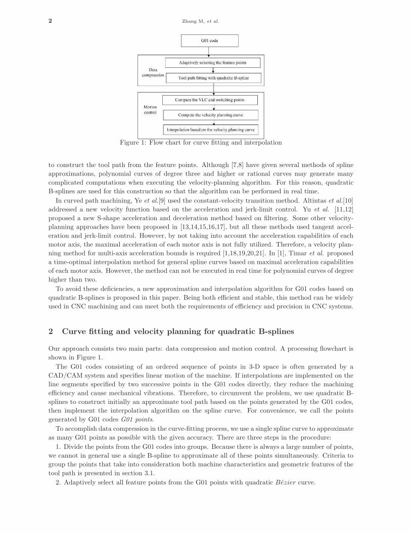
Figure 1: Flow chart for curve fitting and interpolation

to construct the tool path from the feature points. Although [7,8] have given several methods of spline

approximations, polynomial curves of degree three and higher or rational curves may generate many

complicated computations when executing the velocity-planning algorithm. For this reason, quadratic

B-splines are used for this construction so that the algorithm can be performed in real time.

In curved path machining, Ye et al.[9] used the constant-velocity transition method. Altintas et al.[10]

addressed a new velocity function based on the acceleration and jerk-limit control. Yu et al. [11,12]

proposed a new S-shape acceleration and deceleration method based on filtering. Some other velocity-

planning approaches have been proposed in [13,14,15,16,17], but all these methods used tangent accel-

eration and jerk-limit control. However, by not taking into account the acceleration capabilities of each

motor axis, the maximal acceleration of each motor axis is not fully utilized. Therefore, a velocity plan-

ning method for multi-axis acceleration bounds is required [1,18,19,20,21]. In [1], Timar et al. proposed

a time-optimal interpolation method for general spline curves based on maximal acceleration capabilities

of each motor axis. However, the method can not be executed in real time for polynomial curves of degree

higher than two.

To avoid these deficiencies, a new approximation and interpolation algorithm for G01 codes based on

quadratic B-splines is proposed in this paper. Being both efficient and stable, this method can be widely

used in CNC machining and can meet both the requirements of efficiency and precision in CNC systems.

2 Curve fitting and velocity planning for quadratic B-splines

Our approach consists two main parts: data compression and motion control. A processing flowchart is

shown in Figure 1.

The G01 codes consisting of an ordered sequence of points in 3-D space is often generated by a

CAD/CAM system and specifies linear motion of the machine. If interpolations are implemented on the

line segments specified by two successive points in the G01 codes directly, they reduce the machining

efficiency and cause mechanical vibrations. Therefore, to circumvent the problem, we use quadratic B-

splines to construct initially an approximate tool path based on the points generated by the G01 codes,

then implement the interpolation algorithm on the spline curve. For convenience, we call the points

generated by G01 codes G01 points.

To accomplish data compression in the curve-fitting process, we use a single spline curve to approximate

as many G01 points as possible with the given accuracy. There are three steps in the procedure:

1. Divide the points from the G01 codes into groups. Because there is always a large number of points,

we cannot in general use a single B-spline to approximate all of these points simultaneously. Criteria to

group the points that take into consideration both machine characteristics and geometric features of the

tool path is presented in section 3.1.

2. Adaptively select all feature points from the G01 points with quadratic Bezier curve.

Zhang M, et al. Sci China Inf Sci January 2010 Vol. 53 No. 1 3

3. Finally, we use quadratic B-splines to interpolate between all the feature points to obtain a smooth

curved tool path.

After constructing the curved tool path, we begin the velocity planning and real-time interpolation,

so that we can obtain the time-optimal interpolation algorithm. There are also three main steps to this

process.

1. According to how the machine performs and the properties of the fitting tool path, the velocity limit

curve(VLC) together with the switching points (definitions are ginven in later sections) are computed.

2. Given these velocity switching points, the control axis of each switching points and the VLC, the

actual velocity curve is calculated.

3. Using this actual velocity curve and the interpolation tolerance, the interpolating points are com-

puted one by one.

3 Fitting the G01 points with quadratic B-splines

In this section, we discuss in detail the method by which we group the G01 points, select the feature

points and fit the tool path with quadratic B-splines.

3.1 Grouping the G01 codes

In most CNC machining, there is always a large amount of G01 codes for one part program, which can

not be approximated by only a single B-spline curve. Hence, we have to partition these G codes into

groups such that the points of each group can be fitted by a single B-spline curve.

To begin, we must check the distance between every pair of adjacent points against a threshold value

which is set by the properties of the workpiece. If the distance is larger than this value, we keep the line

segment between these two points, which are called breaking points.

In CNC machining, efficiency and accuracy are conditioned one by the other. To meet accuracy

requirements, the velocity of the cutting tool has to decrease when it approaches corners. In particular,

when the curvature of a corner is very high, i.e. indicating a sharp corner, we have to treat the corner

point as a breaking point to maintain fitting errors below the tolerance levels of the system. This indicates

that we must partition the G01 points based on the corresponding discrete curvature and then decide

on the threshold value for curvature taking into account the mechanical properties of the machine. If

a point’s discrete curvature exceeds the threshold value, the corresponding point must be treated as a

breaking point.

According to the method proposed in [22], the discrete curvature of the mid-point of three adjacent

points can be computed. After obtaining the discrete curvatures of all G01-code points, the points with

extreme curvatures are selected and classified as initial feature points.

Let aN be the acceleration on the normal direction of the curve, v the velocity of machining, κ the

curvature, and r the radius of the curve. Because r = v2

aN

= 1κ, the largest curvature of the tool path

that ensures the tool moving smoothly is :

κmax =aNmax

v2(1)

This κmax could conceivably be the curvature threshold value. If there are initial feature points for which

the associated curvature exceeds the threshold value, these would be classified as breaking points.

However, this threshold value does not always work well in all situations. When the machining speed

is not constant, this procedure will not give a stable threshold value. Therefore, we use an estimated

value that is given by the mechanical properties and the processing mode. When the discrete curvature

of the initial feature points satisfies the following condition, these points would be classified as breaking

points:

κ > κmax = αamax

F 2(2)

4 Zhang M, et al.

where amax is the combined acceleration of all axes, F is the given feedrate that is the maximal machining

velocity specified by the system, and α is a rational coefficient that is obtained emirically. In this paper,

we use α = 4 or 9.

3.2 Adaptively selecting the feature points

Having performed the classification, every group of G01-code points can now be approximated by just

one B-spline, recalling that this increases the efficiency of the machining. In most cases, a group may still

contain a large number of points. If going through every point [4,5,23], the fitting curve may comprise

of substantially-many short polynomial curves and take on an unexpected shape [24]. To avoid such

drawbacks, we proposed an adaptive method to select first only the feature points from the G01-code

points, and then use the quadratic B-spline to interpolate all of these feature points. There are two main

steps constituting this adaptively selecting feature points algorithm:

Starting between two breaking points, compute the discrete curvature of every data points using the

method described in Section 3.1. Find the points exhibiting extreme curvature and classify them as initial

feature points.

Next, use the quadratic Bezier curve to add the new feature points. Let the input of the initial feature

points be {Pi1, . . . , Pir} , where Pi1, Pir are two breaking points. The quadratic Bezier curve has the

form:

B(u) = (1 − u)2Q0 + 2u(1 − u)Q1 + u2Q2 (0 6 u 6 1)

where u(∈ [0, 1]) is the affine parameter and Q0, Q1, Q2 are the control points that determine the curve.

Using the quadratic Bezier curve to interpolate every triplet of adjacent feature points {Pij−1, Pij , Pij+1},

we have Q0 = Pij−1, Q2 = Pij+1, u0 = 0, u2 = 1. Using the cumulative chord length method to compute

u1, we get the linear equation for Q1. We have then obtained the quadratic Bezier interpolation curve

B(u).

After obtaining the Bezier curve, we want to find the original positions of Pij−1 and Pij+1 in the

G01 point sequence. We calculate the distances of all the data points between Pij−1 and Pij+1, except

for Pij , to the Bezier curve. If all distances meet the accuracy requirement of the system, then no new

feature point needs to be added. Otherwise, the point furthest away must be added to the feature-point

sequence.

Repeat the procedure until Pir = Q2 and all distances computed from the corresponding points to this

curve meet accuracy requirements given for the system. We then obtain a new sequence of feature points

{Pi1, . . . , Pir′}.

As illustrated in Figure 2, figure (a) is a subsequence of G01 points represented by ◦ . Two end-points

presented by + are breaking points which satisfy condition (2). In figure (b), the points designated by

2 are extreme-curvature points that become initial feature points; the curve in figure (c) is the quadratic

Bezier curve interpolating the three adjacent initial feature points (only one segment is shown for which

a new feature point needs to be added), the point indicated by ⋄ is one for which the distance to the

curve is larger than the error tolerance for the system. So this point will be added to the sequence of

feature points. The tool path illustrated by the quadratic B-spline interpolating all the feature points is

depicted in figure (d) . As we can see in the figure, the adaptive method based on selecting all the feature

points has performed well in capturing the characteristics of the tool path.

Algorithm 1: Adaptively selection of the feature points

Input: A sequence of feature points between two breaking points {Pi1, . . . , Pir}, where Pi1, Pir are the

breaking points.

Output: A new sequence of feature points NewPi = {Pi1, . . . , Pir′}.

Let {Q1, Q2, Q3} be the set of adjacent feature points which will be interpolated by a quadratic Bezier

curve. Let Q1 = Pi1, Q2 = Pi2, Q3 = Pi3.

Let NewPi be the new sequence of feature points, and the initial value is NewPi = {Pi1, . . . , Pir}.

1) Use the Bezier curve to interpolate {Q1, Q2, Q3} so as to generate the curve B(u).

2) Find the original positions of {Q1, Q2, Q3} in the G01 point sequence, and then compute the

distances from all points between Q1 and Q3 to B(u) except for Q2.

Zhang M, et al. Sci China Inf Sci January 2010 Vol. 53 No. 1 5

–4

–3.5

–3

–2.5

–2

48.5 49 49.5 50 50.5 51 51.5

(a) A section of G01 codes between two breaking

points

–4

–3.5

–3

–2.5

–2

48.5 49 49.5 50 50.5 51 51.5

(b) Curvature extreme points

–4

–3.5

–3

–2.5

–2

48.5 49 49.5 50 50.5 51 51.5

(c) Adaptively adding new feature points

–4

–3.5

–3

–2.5

–2

48.5 49 49.5 50 50.5 51 51.5

(d) Quadratic B-spline fitting

Figure 2: Adaptive quadratic B-spline fitting

3) If the maximal distance is larger than the error tolerance, then the corresponding point Pk is

selected. If its position in the G01-code sequence is before Q2, then let Q3 = Q2, Q2 = Pk; Otherwise,

Q3 = Pk; return to 1

4) If Q2, Q3 are not in NewPi, then add them into the feature points sequence NewPi one by one.

5) If Q3 6= Pir , let the next adjacent point of Q3 in NewPi be Pnext, then let Q1 = Q2, Q2 =

Q3, Q3 = Pnext, return to 1.

3.3 Tool path fitting with the quadratic B-splines

The quadratic B-spline can be expressed as:

C(u) =

n∑

i=0

QiNi2(u), 0 6 u 6 1 (3)

where Qi (i = 0, 1, . . . , n) are the n + 1 control points, N i2(u) (i = 0, 1, . . . , n) are the basis functions

defined on the knot vector T = {t0, t1, . . . , tn+3} , which are the subintervals for the spline curve and

u is the affine parameter.

According to the spline interpolation, a system of linear equations in the unknown control points can

be constructed using the corresponding feature points. Because of the properties of quadratic B-splines,

the coefficient matrix is triangular that can be solved by using the chasing method.

Thus by employing the quadratic B-spline to implement the curve-fitting procedure on the G01 point

sequence, a calculation involving triangular coefficient matrix has a higher computing efficiency than

a general system solved by Gaussian elimination [5,25]. Moreover, we can significantly simplify the

calculation involved in the velocity planning procedure.

3.4 Algorithm

Finally, we present the adaptive quadratic B-spline fitting algorithm for the G01 point sequence.

6 Zhang M, et al.

–4

–3.5

–3

–2.5

–2

–1.5

–1

–0.5

0 20 40 60 80 100

Figure 3: Fitting result

Algorithm 2: Adaptive quadratic B-spline fitting algorithm

Input: G01 point sequence {P0, . . . , Pn}.

Output: The set of quadratic B-splines {C1(u), . . . , Cm(u)} as the fitting curve.

1. Compute the curvature threshold value κmax as in (2).

2. Compute the discrete curvature κi (i = 0, . . . , n) with respect to every point in the G01 point

sequence. Take the extreme-curvature points as the initial feature points, and classify as breaking

points for which the curvature is larger than κmax.

3. For the feature point sequence {Pi1, . . . , Pir}, that lie between two breaking points, use the adaptive

selecting method given in Section 3.2 to generate the new feature point sequence {Pi1, . . . , Pir′}.

4. Use the quadratic B-spline to interpolate all the selected feature points to construct the curved tool

path Ci(u) as described in Section 3.3.

Figure 3 is the curve-fitting result of a tool path along the “vase” workpiece in Figure 9. It contains

486 data points, and has been approximated by 34 B-splines including 173 quadratic polynomials. To

show details more clearly, we have expanded the y-coordinate. So the compression ratios are 14.3 or 2.8

according to either for B-spines or quadratic polynomials respectively.

4 Time-optimal machining algorithm based on quadratic B-splines

In the following, we consider 3D spline curves. Before the interpolation step, we need to know the

velocities for all parameters. The procedure that solves this problem is called velocity planning for which

we need to analyze local properties of the curve. Let ′ denote the derivative with respect to u, and ˙ the

derivative with respect to time t.

We assume that the parametric curve C(u) is expressed in the form given in equation (3). Let the

parameter speed of the curve be σ(u) = dsdu

= |C′(u)|. Because v(u) = ds(u)dt

, ddt

= dsdt

duds

ddu

= vσ

ddu

. Our

goal is to compute the velocity curve v(u) = dsdt

that minimizes the traversal time:

minv(u)

T =

∫ T

0

dt =

∫ 1

0

σ

vdu, (4)

Zhang M, et al. Sci China Inf Sci January 2010 Vol. 53 No. 1 7

subject to

|ax(u)| 6 Ax, |ay(u)| 6 Ay, |az(u)| 6 Az, ∀u ∈ [0, 1], (5)

where (ax, ay, az) denotes the acceleration vector in Cartesian coordinates, and (Ax, Ay, Az) denotes the

maximal acceleration allowed.

4.1 Improved velocity planning method for quadratic B-splines

To solve the optimization problem (4), Timar et al.[1] proposed an algorithm based on a ”bang-bang”

control strategy, that is, there is always one axis that attains the acceleration bound. However, this

method involves complicated algebraic equations for high order curves. In this section, we propose an

essential improvement on the algorithm mentioned in [1] for the quadratic B-spline that substantially

reduces the computational requirements.

If we use the “bang-bang” control strategy, we can assume, without loss of generality, that x is the

control axis and therefore ax = ±Ax. Then q′

2σ2 x′ + q

σ3 (σx′′ − σ′x′) = ±Ax. Solving this differential

equation, we have:

q = (σ

x′)2(n ± 2Axx), (6)

where n is a constant that can be computed from a specified point: n = (x′(u∗)σ(u∗) )2q(u∗)∓ 2Axx(u∗). The

above curve q(u) is called the integration curve or integral velocity curve.

Therefore, employing the “bang-bang” control strategy, we need only to find the starting and ending

points, the feedrate at the starting points and the corresponding control axis of the integration curve.

To obtain the starting points of the velocity curve, velocity limit curve(VLC) is introduced in [1], that

is, the curve consisting of the maximal speed limits with respect to every parameter u.

According to the method mentioned in [1], the solution of the VLC has the following form:

v2lim,P,R =

σ2(αRARP ′ − αP AP R′)

P ′R′′ − P ′′R′, (7)

where vlim,P,R denotes the VLC determined by the P and R axes, αP = ±1, αR = ±1, and

P, R ∈ {x, y, z} are two different axes.

To simplify the expression, we use P ,R,M ,N ,K or H to represent one of the x,y and z control axes.

For example, If αP = 1, the corresponding P axis means +P axis; if αP = −1, the corresponding P

axis represents the −P axis; and AP represents the maximal accelerating value of P axis. Now, let the

quadratic spline curve for the P axis have the form: P (u) = aP u2 + bP u + cP , where aP ,bP and cP are

the coefficients of second, first and constant terms, respectively.

Suppose the control axis is +P , then we want to find the first intersection of equation (6) and equation

(7). This means we have to solve a higher-order algebraic equation. Generally, the equation has to be

solved numerically. Taking into consideration of robustness and efficiency of the calculation, meeting

real-time machining requirements is hard to achieve. Thus, for the sake of practicality, we need to avoid

such computation of intersections in the velocity planning curve and the VLC calculations.

Because P and R could be any two of the x,y or z axes, the final VLC is the smallest one of all the

VLCs computed from any two axes. Therefore,

v2lim = min

P,R∈{x,y,z}(v2

lim,P,R). (8)

To do this, we need to explain how to compute the three types of switching points [1] for a quadratic

B-spline.

(i) Tangency points: Because the highest order of the curved path is quadratic, we do not need to

compute the tangent points in our method of computation.

(ii) Discrete points and slope discontinuities of the VLC: For a parameter u, if the left and

right limitation of vlim is different, then we can choose the point with smaller vlim value to be the discrete

point. First, we need to derive the parameter values corresponding to the connection points(breaking

points). These connection points could be the discrete points and slope discontinuities.

8 Zhang M, et al.

When P and R are the control axes, the points where the control axes are changed are possible slope

discontinuities. We can solve the following linear equation to obtain the parameters: α1ARP ′−α2AP R′ =

α′1ARP ′ − α′

2AP R′, where αi, α′i equals ±1, for i = 1, 2.

Another type of slope discontinuity of a VLC can be computed by the intersection points of the VLCs

that are determined by different control axes (P, R) and (M, N)(P, R, M, N ∈ {x, y, z}). The parameter

of the intersection point has the following explicit expression:

u =(αNANbM − αMAM bN )(2aRbP − 2aP bR) − (αRARbP − αP AP bR)(2aNbM − 2aMbN )

(2αRARaP − 2αP AP aR)(2aNbM − 2aMbN) − (2αNANaM − 2αMAMaN)(2aRbP − 2aP bR)(9)

All of the above parameters could be discrete points or slope discontinuities.

We can obtain the final VLC according to equation (8), then check the above parameters to determine

the final discrete points and slope discontinuities.

So, when we employ quadratic B-splines to solve all these three types of switching points, we can

omit the computation of the tangent points and have explicit formulae for both discrete points and slope

discontinuities.

When we compute the integration curve, we have to find the transition points of the control axes where

the control axis has changed. If +P is again the control axis, according to equation (6), we can obtain

the velocity planning curve v2 = ( σP ′

)2(nP + 2AP P ). Solving the acceleration equation of R axis gives:q′

2σ2 R′ + q

σ3 (σR′′ − σ′R′) = ±AR. As a consequence, the parameter of the transition point is a root of a

cubic equation, whose unique real root is:

u =3

√

(aRbP − aP bR)(4aP AP cx + 2aP nP − AP b2P )(aRAP − ARaP )2 + bP aRAP − bP ARaP

2(−aRAP + ARaP )aP

.

Thus, because of the quadratic B-spline, the parameter of the transition point has an explicit expression.

Moreover, we are able to propose an improved velocity planning algorithm.

Algorithm 3: Optimal velocity planning algorithm for quadratic B-spline

Input: Piecewise quadratic B-spline C(u) = (x(u), y(u), z(u))(0 6 u 6 1) with C1 continuity at the

connecting points.

Output: Piecewise velocity-planning curve vsd(u)(0 6 u 6 1).

1. Compute the VLC, the discrete points and the slope discontinuities of the VLC.

2. Starting from u = 0 and initial velocity v(0) = v0, compute the control axis H of this point in the +u

direction. Use H to compute the current velocity curve. As u increases, compute the acceleration

of any non-control axis until it reaches the given bound, that is vv′

σ2 H ′ + v2

σ3 (σH ′′ −σ′H ′) = αKAK ,

where K is any axis except for H. Compute the smallest value of parameter u of the axis transition.

Check whether there exists a switching point such that at least one acceleration bound of the point

is not satisfied. If this is the case, u is set to the smallest parametric value of these switching points.

Recompute the control axis and the new velocity curve according to this parametric value u, the

control axis and current velocity curve; repeat the above procedure until u = 1. Finally, we can

determine the entire velocity curve vF .

Starting from u = 1 and initial velocity v(1) = ve, compute the control axis H in the −u direction.

According to H, compute the current velocity curve. As u decreases, if the acceleration of any

non-control axis reaches the given bound, compute the axis transition parameter u, recompute the

control axis and the new velocity curve until u = 0. Similar to the computation of vF , we finally

determine the velocity-planning curve vB.

3. Compute the intersection point of the forward and backward velocity planning curve vF and vB:

(uin, v(uin)), where v(uin) = vF (uin) = vB(uin). The velocity planning curve is then

vsd(u) =

{

vF , 0 6 u < uin

vB, uin 6 u 6 1.

Zhang M, et al. Sci China Inf Sci January 2010 Vol. 53 No. 1 9

Figure 4: A fitting curveFigure 5: VLC, velocity planning curve, and velocities

at the interpolation points. The unit for the velocities

are mm/s.

Figure 6: Computed acceleration chart of y-axis.

The unit for the acceleration is mm/s2.Figure 7: Computed acceleration chart of z-axis.

The unit for the acceleration is mm/s2.

4. Check whether all switching points of the VLC are under the current velocity planning curve vsd; if

so, then we have obtained the final velocity planning curve vsd, and return vsd; otherwise, continue

the following steps:

5. Select the switching point (usp, vlim(usp)) corresponding to the smallest value of the parameter u for

the current velocity planning curve vsd. Then compute the control axis in the +u and −u directions.

According to this control axis, we can compute two new integration curves vsp−andvsp+, from point

(usp, vlim(usp)) as u decreases and increases, respectively. Then compute (usp−, vsp−(usp−)) and

(usp+, vsp+(usp+)) which are the intersection points of vsp−, vsp+ and the current velocity curve

vsd. Update the whole velocity planning curve vsd as follows:

vsd(u) =

vsd, 0 6 u < usp−

vsp−, usp− 6 u < uin

vsp+, uin 6 u < usp+

vsd, usp+ 6 u 6 1

.

return to step 4.

Remark 4.1. Comparing the above algorithm with that in [1], we have successfully avoided computing

the intersections of the velocity curve and the VLC. However, we have to compute a new velocity planning

curve when the current integration curve exceeds the VLC. In such case, we use a very-high-valued

velocity curve in our algorithm instead of the exceeding part (this part can be checked by comparing

the current velocity and a given upper bound, and if the current velocity exceeds the upper bound, we

define the velocity of the exceeding parts as this value). This is because the final velocity-planning curve

is below the VLC and the exceeding part will be replaced in further computations. This method leads

to the determination of the complete velocity-planning curve and simplifies the computation. The final

actual-velocity curve is composed of the minimal parts of the above velocity curves.

4.2 The interpolation method based on quadratic B-splines

For the given parameter ui, compute the velocity according to the velocity curve vsd, that is, let v(ui) =

min(vsd(ui), vlim(ui)), and then compute the step size ∆L = v(ui) · T (T is the sampling period of the

machine). Use ∆L and the first order approximation to obtain the initial value of the interpolation point.

Next, the Newton-Raphson iteration is employed to approximate the interpolation parameter ui+1[26].

10 Zhang M, et al.

“Vase” workpiece “Beijing Olympic Games”

workpiece

“Head-sculpture” workpiece

Figure 8: Workpieces

“Vase”-NC machining picture Machine picture

Figure 9: Machining examples

4.3 Computational simulations

The fitting curve chosen for illustration is one of the tool paths in the “vase” workpiece in Figure 8.

As seen in Figure 4, this curve is composed of 6 piecewise quadratic B-spline, and has C1 continuity

at the connecting point. The G01 point sequence is constructed by the cutting plane method, and as a

consequence, there is only y- or z-axis control of the machining. The acceleration bounds of the control

axes are Ay = 3000mm/s2 and Az = 1000mm/s2. After the computation, we obtain the VLC and the

velocity planning curve as displayed in Figure 5, the discontinues curve at the top of Figure 5 is the VLC,

the continuous curve is the velocity planning curve, the circles are the actual computed velocities of the

interpolation points. The actual computed accelerations along the y- and z-axes are shown in Figures 6

and 7, respectively. From this, it can be seen that the actual machining is controlled basically under the

optimal “bang-bang” control strategy.

5 Experimental results

To test the algorithms presented above, three workpieces for actual machining are chosen: i.e., “vase”,

“Beijing Olympic Game”, and “head sculpture”, which are depicted in Figure 8. In Figure 9, we give the

picture of the NC machine used in our experiments and two real “vase” manufactured in the NC machine

with our method. The “Beijing Olympic Games” workpiece is a simple model compared with the others,

but the “vase” is very complicated, which is typical of bi-axis machining. The “head sculpture” is highly

representative of three axis machining. All simulations were performed on a PC with 2.13GHz Intel Core

Zhang M, et al. Sci China Inf Sci January 2010 Vol. 53 No. 1 11

2 processor using the VC++6.0 environment.

Employing the algorithm addressed in Section 2, we computed the spline compression ratio(the number

of line segments approximated by one spline curve) for each workpiece; these were 27.3, 156.3, and 74

for “vase”, “Beijing Olympic Games” and “head sculpture” workpiece, respectively. The polynomial

compression ratio (the number of line segments approximated by one polynomial) of these three were

3.6, 15.5, and 8.1 respectively. We next used Algorithm 3 proposed in Section 4 to perform velocity

planning and interpolation. Comparing the results with the const velocity transition method [8], our

computing efficiency improved by 65%− 130%. Compared the results with the traditional arc transition

interpolation method, our computing efficiency improved by 30% − 110%.

In regard to the computation times, the time spent on constructing the tool path can be neglected

compared with that associated with velocity planning and interpolation. The computation time in per-

forming the improved velocity planning method and interpolation method are almost the same, but are

much less than the machining time. This means that these computations can be conducted in real time.

From the simulations, we can see that the algorithms we have proposed have worked well for both

simple (“Beijing Olympic Games”) and complicated (“vase” and “head sculpture”) examples.

The machining examples show that our algorithm is practical and robust.

6 Closing remarks

The optimal velocity-planning and interpolation algorithms proposed in this paper are based on the

quadratic B-splines. We used an adaptive method to select all feature points from the G01 point sequence,

and then used quadratic B-splines to interpolate between all these feature points. From the point of view

of simulations, this data-compression method is very efficient, accurate, and stable, and also can be widely

used in CNC machining.

For quadratic B-splines, we proposed an efficient algorithm to compute actual-velocity curves within

the “bang-bang” control strategy. In the computing procedure, we have made full use of the properties

of quadratic B-splines. Our improved method mainly has resolved the following problems:

1. The computation of intersections of velocity curves and VLC is circumvented, thereby eliminating a

large amount of computation that would have been necessary in solving the high-order algebraic equations.

2. Employing quadratic B-splines has reduced a number of computing steps and avoided the occur-

rence of the high-order equation. Essentially, we can obtain all solutions explicitly. Thus circumventing

complicated computations arising from employing numerical methods.

However, our method is based on considering a complete curve over the workpiece; the velocity at its two

end-points must be specified. If we want to increase the machining velocity, we have to introduce global

methods to plan the velocities at the end-points. Such global methods will involve a lot of backtracking

computation which may lower the efficiency. With this in mind, we will be focusing on local methods

in future research, particularly in regard to velocity planning at the end-points, so as to maintain global

optimal control and to achieve real time interpolation within the accuracy required.

Acknowledgements

This work was supported by Knowledge Innovation Project of The Chinese Academy of Sciences (Grant No.

KGCX2-YW-119-1), and NSFC (Grant No. 608210021/F02). The authors would like to thank Shenyang Institute

of Computing Technology, Chinese Academy of Sciences for their kind help to implement our algorithm in their

machine and to manufacture “Vase” workpiece.

References

1 Sebastian D T, Farouki R T, Smith T S, Boyadjieff C L. Algorithms for time−optimal control of CNC machines along

curved tool paths. Robotics and Computer-Integrated Manufacturing, 2005, 21(1), 37-53

12 Zhang M, et al.

2 Lv Q, Zhang H, Yang K M, Ye P Q. Study on the method of increasing turning velocity during CNC continuous

machining (in Chinese). Manufacturing technology and Machine Tool, 2008, 3(7), 79-83

3 Zhang L X, Sun R Y, Gao X S, Li H B. An optimal solution for high-speed interpolation of consecutive micro-line

segments and adaptive real-time lookahead scheme in CNC machining(in Chinese). MM-Preprints, 2010, (29), 206-227

4 Yau H T, Wang J B. Fast Bezier interpolator with real-time lookahead function for high-accuracy machining. Interna-

tional Journal of Machine Tools and Manufacture, 2007, 47(10), 1518-1529

5 Wang J B, Yau H T. Real-time NURBS interpolator:application to short linear segments. International Journal of

Advanced Manufacturing Technology, 2009, 41(11), 1169-1185

6 Zhao X, Yin Y, Yang B. Dominant point detecting based non-uniform B-spline approximation for grain contour. Science

in China Ser.E Technological Sciences, 2007, 50(1), 90-96

7 Farin G, Hoschek J. Handbook of Computer Aided Geometric Design, Elsevier Science, 2002

8 WANG R H. Numerical rational approximation (in Chinese). Shanghai Science and Technology Press, 1980.

9 YE P Q, Zhao S L. Study on control algorithm for micro-line continuous interpolation (in Chinese). China Mechanical

Engineering, 15(15), 1354-1356

10 Erkorkmaz K, Altintas Y. High speed CNC system design. Part I: jerk limited trajectory generation and quintic spline

interpolation. International Journal of Machine Tools and Manufacture, 2001, 41(9), 1323-1345

11 Yu D, Hu S H, Gai R L, Bai Z W. Research on acceleration and deceleration for CNC machine tools based on filtering

(in Chinese). China Mechanical Engineering, 2008, 19(7), 804-807

12 Gai R L, Lin H, Zheng L M, Huang Y. Design and implementation of velocity planning algorithm for high speed

machining (in Chinese). Journal of Chinese Computer Systems, 2009, 30(6), 1067-1071

13 Shi C, Zhao T, Ye P Q, Lv Q. Study on S-shape curve acceleration and deceleration control on NC system (in Chinese).

China Mechanical Engineering, 2007, 18(12), 1421-1425

14 Du D S, Yan C L, Li C X. An adaptive NURBS interpolator with real-time look-ahead function (in Chinese). Journal

of Shanghai Jiaotong University, 2006, 40(5), 843-847

15 Lin M T , Tsai M S, Yau H T. Development of a dynamics-based NURBS interpolator with real-time look-ahead

algorithm. International Journal of Machine Tools and Manufacture, 2007, 47(15), 2246-2262

16 Liu X S, Jia Q X, Yuan X H. A study of NURBS interpolation algorithm and ACC-DEC control (in Chinese). Modular

Machine Tool and Automatic Manufacturing Technique, 2007, 2(11), 60-64

17 Yuan C M, Gao X S. Time-Optimal Interpolation of CNC Machines along Parametric Path with Chord Error and

Tangential Acceleration Bounds. MM-Preprints, 2010, (29), 165-188

18 Zhang K, Gao X S, Li H B, Yuan C M. A Greedy Algorithm for Feed-rate Planning of CNC Machines along Curved

Tool Paths with Confined Jerk for Each Axis. MM-Preprints, (29), 189-205

19 Bobrow J E, Dubowsky S, Gibson J S. Time-optimal control of robotic manipulators along specified paths. International

Journal of Robotics and Automation, 1985, 4(3), 3-17

20 Shiller Z, Lu H H. Robust computation of path constrained time optimal motions. Proceedings, IEEE International

Conference on Robotics and Automation, Cincinnati, OH, 1990, 144-149

21 Timar S D, Farouki R T. Time-optimal traversal of curved paths by Cartesian CNC machines under both constant and

speed-dependent axis acceleration bounds. Robotics and Computer-Integrated Manufacturing, 2007, 23(2), 563-579

22 Coeurjolly D, Svensson S. Estimation of curvature along curves with application to fibres in 3d images of paper. Lecture

notes in computer science, 2003, 2749(1), 247-254

23 Lin H, Wang G, Dong C. Constructing iterative non-uniform B-spline curve and surface to fit data points. Science in

China Ser.F Information Sciences, 2004, 47(3), 315-331

24 Piegl L, Tiller W. The NURBS books, Springer, Berlin, 1997

25 Kang S J, Zhou L S, Zhang D L. Fitting cutter location points with B-spline curves accurately (in Chinese). Mechancal

Engineering and Automation, 2007, 262, 95-97

26 Shi R M. Numerical Computation (in Chinese), Advanced Education Press, 2004