curve fitting with confidence for preclinical dose

CURVE FITTING WITH CONFIDENCE FOR PRECLINICALDOSE–RESPONSE DATA

MATHIAS CARDNER

Abstract. In the preclinical stage of pharmaceutical drug development, when investigatingthe medicinal properties of a new compound, there are two important questions to address.The first question is simply whether the compound has a significant beneficial effect comparedto vehicle (placebo) or reference treatments. The second question concerns the more nuanceddose–response relationship of the compound of interest. One of the aims of this thesis isto design an experiment appropriate for addressing both of these questions simultaneously.Another goal is to make this design optimal, meaning that dose-levels and sample sizes arearranged in a manner which maximises the amount of information gained from the experiment.We implement a method for assessing efficacy (the first question) in a modelling environmentby basing inference on the confidence band of a regression curve. The verdicts of this methodare compared to those of one-way anova coupled with the multiple comparison procedureDunnett’s test. When applied to our empirical data sets, the two methods are in perfectagreement regarding which dose-levels have an effect at the 5% significance level. Throughsimulation, we find that our modelling approach tends to be more conservative than Dunnett’stest in trials with few dose-levels, and vice versa in trials with many dose-levels. Furthermore,we investigate the effect of optimally designing the simulated trials, and also the consequencesof misspecifying the underlying dose–response model during regression, in order to assess therobustness of the implemented method.

Key words: pharmacodynamic modelling; efficacy study; dose–response; optimal design;model-robust design; simultaneous confidence bands; bootstrap; multiple comparisons

Date: January 21, 2015.Thesis for the degree of Master of Science, written in the field of mathematical statistics as part of the two-

year Master’s Programme in Mathematical Sciences at the University of Gothenburg in Sweden. Please directcorrespondence to [email protected]

Supervisor: Sofia Tapani, PhD, Senior Statistician, Discovery Statistics, AstraZeneca R&D in Mölndal.Co-advisor: Rasmus Jansson Löfmark, PhD, CVMD iMed DMPK, AstraZeneca R&D in Mölndal.Examiner: Professor Aila Särkkä, Department of Mathematical Sciences, Chalmers University of Tech-

nology and the University of Gothenburg.

2 MATHIAS CARDNER

Acknowledgements

I want to express my deep gratitude to my supervisor Sofia Tapani for her skilfulguidance and insightful advice. Likewise, I am very thankful to my co-advisorRasmus Jansson Löfmark for many stimulating discussions, and for giving mea better understanding of pharmacological concepts. I would also like to thankMarita and Janeli for fantastic company, interesting conversations, and resourcesboth computational and literary.

Many important ideas in this thesis were inspired by a presentation whichMarianne Månsson, Karin Nelander and Marita Olsson gave at Statistikerträffenin September of 2012. Furthermore, I have received highly valuable commentsand suggestions from Pete Ceuppens, Brian Middleton and Marie South, whichgreatly enhanced the results of this thesis.

Finally, I would like to express my appreciation for the library at ChalmersUniversity of Technology and its staff. The library has been a tremendous asset,without which I would likely not have gained access to the splendid sources ofinformation upon which this thesis rests.

Contents

1. Introduction 31.1. Background 31.2. Pharmacological background 41.3. Reading guide 4

2. Data exploration and modelling 52.1. Data 52.2. Mathematical models 9

3. Literature review 104. Theory 124.1. Optimal design of experiments 124.2. Nonlinear regression 154.3. Construction of confidence bands 16

5. Implemented method 216. Results and discussion 246.1. Simulations 246.2. White book 28

7. Conclusions 29Future work 30

References 31

CURVE FITTING WITH CONFIDENCE FOR PRECLINICAL DOSE–RESPONSE DATA 3

1. Introduction

1.1. Background. During the early development of a medicinal drug — when investigatingwhether a certain compound has some beneficial effect — there are traditionally two differentstrategies behind the statistical analyses performed [1]. The first strategy — which we shallrefer to as an efficacy study — is designed to determine, with statistical significance, whetherthe compound actually does have a beneficial effect compared to control or reference treatments.This design typically has relatively few dose-levels, with many observations made at each levelin order to yield statistical confidence in the results. The other strategy, which is model-basedin nature, is geared towards gaining more nuanced information about the dose–response profileof the compound of interest [2]. This design typically has a larger number of dose-levels, spreadout in such a way that we gain insight into the mechanistic (functional) form of the underlyingphenomena, whilst sacrificing confidence by having fewer observations at each dose-level. It isimportant to keep in mind that the total number of observations is limited by available resourcesand, in the case of in vivo studies, by ethical considerations since animals are involved. Themajor benefit of this model-based approach is that it can be used to estimate appropriate dose-levels for future studies. If the target dose is incorrectly estimated, the recommended dose-levelfor subsequent trials may be set too high, potentially causing concerns of toxicity and safety.Alternatively, if the recommended dose-level is set too low, its beneficial effect may be too smallto detect in a confirmatory phase [3].

The overarching goal of this project is to devise a strategy for a statistical analysis whichaddresses both of the above questions simultaneously. In other words, we aim to design anexperiment which lends insight both into the efficacy and the dose–response relationship of agiven compound. The most obvious reward is that of parsimony, since a successful synthesis ofthe traditionally disparate experiments would save resources — both financially and ethically.Moreover, it would be of value to experimenters who wish to gauge the mechanistic dose–responserelationship whilst retaining statistical confidence in the results. Say for instance that a researcheris primarily interested in estimating the minimum effective dose (MED), defined as the smallestdose which yields a clinically relevant and statistically significant effect [4]. Then an experimentaldesign could be optimised with respect to its ability of estimating the MED, in the sense ofminimising the variance of this estimate [5]. The methodology derived from our investigations willbe summarised in Section 6.2 as a guide for designing and analysing dose–response experiments.

Further nuance. It is worthwhile to make a few observations about the fundamental differencesbetween the two types of strategies mentioned above. In the efficacy study, the dose-levels areconsidered to be qualitative, and the statistical analysis (e.g. anova) requires comparatively fewassumptions [1]. Conversely, in the model-based approach, assumptions must be made concerningthe underlying model of dose–response, which then describes a functional relationship betweenthe dose — now viewed as inherently quantitative — and the response. If the postulated modelis representative of the true dose–response relationship, then this more nuanced knowledge cananswer important questions. For instance, it can be used to estimate the dose which attains halfthe maximal effect (ED50) or the minimum effective dose (MED) [3]. Thus, whereas inferencefrom the efficacy study is limited to the dose-levels at which observations were made, the model-based approach can be used to interpolate the response within the range between the smallestand largest dose administered (including the vehicle treatment). This increased flexibility comesat the cost of more assumptions, which, if unrepresentative of the true phenomena, may yieldmisleading results.

Granted, when an experiment has been performed and the measurements have been gathered,there is nothing preventing us from using both of the above methodologies to analyse the data.Notice that it is the experimental design (i.e. the arrangement of dose-levels and their sample

4 MATHIAS CARDNER

sizes) which may make one of the methods more appropriate than the other. In light of this, animportant objective of this thesis is to investigate how the allocation of experimental resourcesaffects the inferences drawn from the different methodologies.

1.2. Pharmacological background. This thesis focuses on dose–response studies, in which adrug is administered at various dose-levels and the corresponding response is measured. Themedicinally active substance is delivered in an inert substance (excipient) referred to as vehicle.In order to measure the null effect — i.e. to establish a baseline response — it is appropriateto include a treatment containing no active substance, but only the vehicle itself. This vehicletreatment is a control expected to have no effect, and as such, it can be thought of as a type ofplacebo. Since the vehicle treatment contains no trace of the active substance, it is appropriate toassociate it with a dose-level of zero. Furthermore, the dose-levels are generally spread out moreor less evenly on a logarithmic scale, in order to gauge the response across orders of magnitude.Hence it is often appropriate to use a logarithmic transformation on the dose scale when plottingthe data. This however causes trouble with the vehicle, since the logarithm of zero is not (finitely)defined, meaning that it is not obvious how to handle the vehicle treatment. One possible solutionis to adjust the response so that it becomes relative to the estimated baseline — for instanceby uniformly subtracting the mean vehicle response. We have not done this in the upcomingfigures, where the plots with a logarithmic dose scale simply omit the vehicle treatment. It will,however, play an important role in accounting for the variability in the mean vehicle responsewhen we implement our method in Section 5.

1.3. Reading guide. As this thesis is written in the field of mathematical statistics applied topharmacology, it is intended for two audiences with different backgrounds. Since the author’sknowledge of pharmacology was virtually nonexistent at the beginning of this project, the thesisshould hopefully be self-contained with respect to the pharmacological concepts involved. Thesame can however not be said of its mathematical and statistical contents, which will primarilyappeal to those already acquainted with those fields. Therefore, we shall here offer a readingguide intended to outline the topics most relevant to the reader without a statistical background.

In Section 2 we describe empirical dose–response data sets which set the stage for the subse-quent analysis. This leads to Section 2.2 in which we introduce common dose–response models.The literature review in Section 3 is the result of an extensive search for previous work addressingour problem, albeit rather tangentially. Nevertheless, the fruits of this search include articlesand software which are highly useful for model-robust optimal design of dose–response trials.

Section 4 contains the mathematical and statistical methods we use throughout this thesis.It begins with the theory of optimal design of experiments, which, given some postulated dose–response model, determines the optimal allocation of experimental resources. In short, thistheory tells us how many dose-levels to include, where to place them, and how many subjectsto assign to each level. Granted, the resulting design will only be optimal from a mathematicalpoint of view, and may suggest dose-levels which are inconceivable in practice. This is lateraddressed by software which rather lets the experimenter specify feasible candidate dose-levelsbeforehand, from which the most efficient allocation is chosen.

In Sections 4.2 and 4.3 we discuss regression and the construction of confidence bands aroundregression curves. This leads up to the key result in Section 5 in which we present our methodfor assessing efficacy under a modelling approach. The judgements made by this method arecompared to those of one-way anova coupled with the multiple comparison procedure Dunnett’stest, which controls the family-wise error rate when comparing each dose-level against the vehicletreatment. (See Bretz et al. (2010) [6] for a detailed account of this test.) This is done throughcomprehensive simulations of dose–response trials, the findings of which are presented in Section6 containing our results and discussion. Section 6.2 outlines a method for designing and analysing


dose–response studies using the R [7] package DoseFinding [8]. The conclusions in Section 7 givea summary of our findings, as well as elaborations on avenues of future work.

2. Data exploration and modelling

2.1. Data. Our investigations are supported by data sets containing empirical in vivo dose–response data for three different compounds, referred to as compounds A, B and C. For eachcompound, two response variables have been measured (from the same physical sample). Themeasured response quantities shall for each compound be referred to as response 1 and 2. Note,however, that these responses do not necessarily measure the same quantity for different com-pounds. For instance, response 1 of compound A may measure something different than doesresponse 1 of compound B.

Figures 1–6 display boxplots and scatterplots of all six data sets. Notice that the dose-levelsare logarithmically scaled in the scatterplots, meaning that the zero-dose vehicle treatment isnot included. The data are analysed using one-way anova coupled with Dunnett’s test [6],which adjusts for multiplicity (see Section 4.3) when comparing each dose-level against vehicle.Throughout this thesis we perform Dunnett’s test using the R [7] package multcomp [9]. Wesay that a dose-level is active if it shows a statistically significant effect compared to the vehicletreatment (at the given significance level, which in this thesis is set to 5%). The verdicts ofDunnett’s test are recorded in the figure captions.

6 MATHIAS CARDNER

●

●

●

●

0 0.5 1 2 4 8 10 100

050

100

150

Compound A, response 1

Dose

Res

pons

e

●

●

●

●

●●

●

●●

●●

●

●

●

●

●

●

●

●

●●

●

●

●

●●●●●●

●

● ●

●

●●●

●●

● ●

●

●●●

●●● ●

●

●

●

●●

●

0.5 1.0 2.0 5.0 10.0 20.0 50.0 100.0

050

100

150


Dose (logarithmic scale)

Res

pons

e

MeansMedians

Figure 1. Boxplot (left) and scatterplot (right) of the observed dose–responsedata of compound A with respect to response 1. Dunnett’s test indicates thatthe two highest dose-levels, 10 and 100, are active at the 5% significance level(both with p-values smaller than 0.03%). The data clearly suggest an increasingtrend, with the possible exception of dose-level 1. The spread of the data ateach dose-level is symmetric about its mean, which is generally quite close toits median. These statistics deviate most markedly at dose-level 10, due to ablatant outlier. Furthermore, there is evidence of heteroscedasticity, with largervariability at higher dose-levels — the exception being dose-level 1 whose datais quite variable.

●

0 0.5 1 2 4 8 10 100

5010

015

020

025

030

0


Dose

Res

pons

e

●

●

●

●

●

●

●

●

●

●●

●

●

●

●

●

●

●

●

●

●

●

●

●

●

●●

●

●

●

●●

●

●

●

●

●

●

●

●

●

●

●

●

●

●

●●

●

●

●

●●

●

●

0.5 1.0 2.0 5.0 10.0 20.0 50.0 100.0

5010

015

020

025

030

0



Res

pons

e

MeansMedians

Figure 2. Boxplot (left) and scatterplot (right) of the observed dose–responsedata of compound A with respect to response 2. Dunnett’s test declares noactivity at significance level 5% (nor at 10%). The data indicate no apparenttrend. At each dose-level, the observations are spread symmetrically about themean, which tends to be slightly higher than the median. The heteroscedas-ticity follows no simple pattern, though again the variability at dose-level 1 isconspicuously large.


0 50 150 450

0.4

0.6

0.8

1.0

1.2

Compound B, response 1

Dose

Res

pons

e

●

●

●

●●

●●

●

●

●

●

●

●

●

●

●

●

●

●

●●

●

●

50 100 200

0.4

0.6

0.8

1.0

1.2



Res

pons

e

MeansMedians

Figure 3. Boxplot (left) and scatterplot (right) of the observed dose–responsedata of compound B with respect to response 1. Dunnett’s test declares noactivity at significance level 5% (nor at 10%). The data indicate no monotonictrend. The observations are quite skewed, though not uniformly in the samedirection, which disqualifies a monotone transformation. Heteroscedasticity ap-pears erratic, with high variability in the vehicle treatment and two extremeobservations at dose-level 150.

●

0 50 150 450

24

68

1012


Dose

Res

pons

e

●

●

●

●●

●

●

●

●

●

●

●●

●

●

●●

●●

●

●

●

●

50 100 200

24

68

1012



Res

pons

e

MeansMedians

Figure 4. Boxplot (left) and scatterplot (right) of the observed dose–responsedata of compound B with respect to response 2. Dunnett’s test indicates thatthe highest dose-level, 450, is active at the 5% significance level (with a p-valueof 3%). Aside from the vehicle treatment, there is evidence of a decreasing trend.The observations are fairly symmetrical around the means. Heteroscedasticityis present in that variability appears to decrease with higher dose-levels.

8 MATHIAS CARDNER

●

●

●

0 0.18 0.54 1.8

2025

30

Compound C, response 1

Dose

Res

pons

e

●

●

●

●

●●

●

●

●

●

●

●

●

●

●

●

●

●

●

●

●

●

●

●

0.2 0.5 1.0

2025

30



Res

pons

e

MeansMedians

Figure 5. Boxplot (left) and scatterplot (right) of the observed dose–responsedata of compound C with respect to response 1. Dunnett’s test declares noactivity at significance level 5% (nor at 10%). The data suggest no apparenttrend. The observations are quite symmetrical about the means, with no obviousheteroscedasticity, barring a few outliers.

●

0 0.18 0.54 1.8

010

020

030

040

0


Dose

Res

pons

e

●●

●

●

●

●

●●

●

●

●

●

●

●

●

●

●●●●

●

●

●

●

0.2 0.5 1.0

010

020

030

040

0



Res

pons

e

MeansMedians

Figure 6. Boxplot (left) and scatterplot (right) of the observed dose–responsedata of compound C with respect to response 2. Dunnett’s test indicates that thetwo highest dose-levels, 0.54 and 1.8, are active at the 5% significance level (bothwith p-values smaller than 0.4%). The data clearly indicate a decreasing trend.The observations are slightly positively skewed, perhaps indicating the proprietyof a monotone transformation. Indeed, a logarithmic transformation of theresponse (which, for the sake of brevity, is not shown) does yield a dramaticallymore symmetrical spread around the means. It also alleviates the ostensibleheteroscedasticity, with high variability in the vehicle treatment, as opposed tothe remarkably low variability at dose-level 1.8. The logarithmically transformeddata are however nearly homoscedastic.


2.2. Mathematical models. Throughout this thesis we will consider the functional relationshipbetween an explanatory (predictor) variable x and a response variable y. Denoting the responsefunction by η we will write y = η(x, θ) where θ is a vector containing all parameters of the givenresponse function.

The Emax model and its derivatives. In pharmacodynamic modelling of dose–response relation-ships, one of the most common choices is the so-called Emax model [10] which can be motivatedby using a biological interpretation [11]. Its response, in the case of an increasing dose–responseprofile, is given by

η(x,E0, Emax,ED50) = E0 + Emax · xED50 + x

,

where E0 is the response at dose x = 0 (i.e. the vehicle response), Emax is the maximum effectinduced by the drug, and ED50 is the smallest dose which attains half the maximal effect. Noticethat Emax is the change in response relative to the baseline E0, meaning that the absolutemaximal response is Rmax = E0 + Emax.

The Emax model in the case of a decreasing dose–response relationship is analogous, with theresponse function

η(x,E0, Imax, ID50) = E0 −Imax · xID50 + x

,

where Imax is the maximum inhibition induced by the drug, and ID50 is the smallest dose whichattains half the minimal effect. Henceforth, the inhibitory model will be included in the modelwith an increasing profile by allowing the parameter Emax to be negative.

The Emax model can be extended by raising the dose x and ED50 to a power h, which yieldsthe sigmoid Emax model given by

η(x,E0, Emax,ED50, h) = E0 + Emax · xh

EDh50 + xh

.

The so-called Hill coefficient h is proportional to the slope of η at ED50 — see Gabrielsson andWeiner (2006) [11]. In order to distinguish the two models, the former is sometimes referred toas the hyperbolic Emax model [10].

Perhaps at the expense of biological interpretation, the sigmoid Emax model can be moresuccinctly expressed (by simplifying the quotient) as

η(x,E0, Emax,ED50, h) = E0 + Emax

1 + (ED50/x)h .

This equivalent form of the sigmoid Emax model is referred to as the four-parameter logistic model[12]. Another equivalent form — useful for numerical purposes, or when applying a logarithmictransformation to the dose — is the logistic model


1 + exp[(log ED50 − log x)h] .

Additional dose–response models. Without giving biological interpretations, we shall also employthree dose–response models included in the R [7] package DoseFinding [8] (see the next Section3 for more information about this package). These comprise an exponential model

η(x,E0, E1, δ) = E0 + E1(exp(x/δ)− 1),a linear-in-log model

η(x,E0, δ, offset) = E0 + δ log(x+ offset),and a beta model

η(x,E0, Emax, δ1, δ2, scale) = E0 + EmaxB(δ1, δ2)( x

scale

)δ1(1− x

scale

)δ2,

10 MATHIAS CARDNER

where B(· , ·) is the beta function and “scale” is a fixed dose-scaling parameter. Figure 7 displaysstandardised schematic plots conveying the typical shape of the above mentioned models. Inparticular, this figure reveals the ability of the beta model to capture a non-monotone dose–response profile.

Dose

Mod

el m

eans

0.0

0.2

0.4

0.6

0.8

1.0

●

●

Emax

0.0 0.2 0.4 0.6 0.8 1.0

●

●

Sigmoid Emax

●

●

Logistic

0.0 0.2 0.4 0.6 0.8 1.0

●

●

Linear in Log

●

●

Exponential

0.0 0.2 0.4 0.6 0.8 1.0

0.0

0.2

0.4

0.6

0.8

1.0

●

●

Beta

Figure 7. Standardised schematic plots of common dose–response models. Allmodels are monotonic except for the beta model, which can accommodate anon-monotone dose–response profile. The graphic was created using the R [7]package DoseFinding [8].

3. Literature review

As mentioned above, the aim of this thesis is to combine an analysis of efficacy and a model-based approach. In the former analysis, when investigating the effect of various dose-levels (andvehicle) we traditionally utilise multiple comparison procedures to control the family-wise errorrate. Conversely, the strength of the model-based approach is its potential to give more nuancedinformation about the underlying dose–response relationship. We have followed the work of FrankBretz, José Pinheiro, Björn Bornkamp and Holger Dette (with specific references to follow).

Bretz et al. (2005) [1] devised a strategy for combining multiple comparison techniques withdose–response modelling, introduced in their so-called MCP-Mod methodology. The term is anabbreviation of “multiple comparison procedures with modelling techniques”. Whilst this maysound very similar to the objective of this thesis, the multiple comparisons of which they speakpertain to model selection — not dose-levels. Their method can be used to select from a collectionof candidate models (with specified parameters) the one which most aptly describes a given set


of dose–response data. The fundamental idea is to develop, for each model, a hypothesis testbased on contrasts of the means of the responses at the various dose-levels (including the vehicletreatment). The contrasts for each model are chosen in such a way that if that particular model iscorrect, the chance of rejecting the null hypothesis (of no effect) is maximised. After establishinga critical value for adjusting the family-wise error rate of the multiple hypothesis tests, themodels with significant test statistics can be identified from the candidate set. Subsequently,the winning model is chosen to be the one whose test statistic yielded the smallest p-value(adjusted for multiplicity). This leads to the main advantage of their approach, namely that thewinning model can be used to make inferences beyond the original dose-levels. For instance, itcan be used in dose-finding — that is, to estimate which dose ought to yield a given response.Constructing a confidence band around the curve corresponding to the winning model allows usto judge whether a given dose has a statistically significant effect compared to vehicle. Theyhave implemented this work in the R [7] package MCPMod [13]. Their framework was expoundedupon by Pinheiro et al. (2006) [2] who developed methods for power and sample size calculationsunder this methodology.

It is important to note, however, that their method is concerned with model selection aposteriori whereas we are interested in optimal design of experiments a priori. In other words,MCP-Mod can determine which model best describes a given data set, but our task is to designan experiment before having seen the resulting data. (Indeed, Pinheiro et al. (2006) [2] identifiedthis as an avenue of further research.) Nevertheless, their work will prove beneficial also forour purposes, and the functionality of MCPMod was subsequently subsumed into the R packageDoseFinding [8] written by the same authors. This latter package expands upon the MCP-Modframework by including routines for optimal design, the theory of which was developed by Detteet al. (2008) [5]. In the cited article they show (via simulation) that locally optimal designsdeveloped for common dose–response models — the exponential, linear-in-log, and Emax models— are moderately robust with respect to misspecification of the model parameters, but thatthey are far more sensitive to misspecification of the regression model itself. Their attempt tocircumvent this problem is reminiscent ofMCP-Mod, but rather than focusing on model selection,their analysis is geared toward optimal design of experiments. More concretely, their strategy isbased on considering a collection of relevant candidate models, and choosing the design whichmaximises the minimum efficiency of the designs tailored to the members of that family. Thus,rather than designing for a single model (which may have been misspecified) they search for adesign which is adequate for all candidate models. This makes the design more robust againstmodel misspecifications.

The methodologies discussed thus far allow for the inclusion of a vehicle treatment, but Detteet al. (2014) [14] describe a method which in addition incorporates an active control. This maybe a reference treatment — for instance a compound by a competitor — against which thecompound under investigation is to be compared. It may also be a medical condition whichthe drug is meant to alleviate. Time has not permitted us to investigate this scenario, but itnevertheless provides a compelling avenue for further research.

12 MATHIAS CARDNER

4. Theory

4.1. Optimal design of experiments. In this section we shall briefly outline the theory ofoptimal experimental design needed for the purposes of this thesis. We will follow Fedorov andLeonov (2013) [12] in the formulation of the theory, but much inspiration has also been drawnfrom Atkinson et al. (2007) [15]. The following will necessarily be technically involved, but looselyspeaking, optimal design theory is concerned with determining where to make measurements —and how many to make at each point — in order to gain as much information as possible fromthe experiment. This latter condition will depend on the criterion of optimality, but one commonchoice is the D-criterion, in which points of measurement are selected in such a way that, givensome postulated model, the variance of its estimated parameters is minimised. For our purposes,when fitting for instance an Emax model, a D-optimal design ensures that the estimates of E0,Emax and ED50 will be as precise as possible — provided that the underlying dose–responserelationship can be accurately represented by an Emax model.

Consider an experiment whose response function η(x, θ) depends on the parameter vectorθ ∈ Rm containing m parameters. The predictor x belongs to the design region X ⊆ Rk. (Forthe purposes of this thesis, k = 1 since x is a univariate measure of dose.) For i = 1, . . . , nlet there be ri replications made at design point (dose-level) xi ∈ X and thus N =

∑ni=1 ri

observations in total. An exact design

ξN ={x1 · · · xnp1 · · · pn

}where pi = ri/N

is a probability measure on X . Thus a design ξN = {xi, pi}ni=1 is simply a collection of supportpoints xi ∈ X and their corresponding weights pi (which sum to unity).

A design is referred to as exact if the weight of the ith support point is pi = ri/N . A continuousdesign ξ = {xi, pi}n1 is one in which each pi can be any real number in [0, 1] under the constraintthat

∑i pi = 1. In practice, all designs are of course exact (since the number ri of measurements

must necessarily be an integer). However, the ensuing optimisation problem in the discrete caseis much more complex than its continuous counterpart. Therefore, in order to harness the powerof convex optimisation theory, we shall focus on continuous designs. When having found theoptimal continuous design ξ for some problem, this can be trivially approximated to yield theoptimal exact design ξN .

The linear response model. The purpose of optimal design of experiments is to strategicallydetermine the design points xi ∈ X and their corresponding weights pi. The optimal allocationof design points xi will of course depend on the underlying model, so we must make an assumptionabout the response function η(x, θ). We shall begin by investigating the linear model η(x, θ) =θ>f(x) where θ = (θ1, . . . , θm)> contains the m parameters and f(x) = [f1(x), . . . , fm(x)]>contains the m base functions. (Thus the model is linear with respect to the parameters, whereasthe base functions need not be linear.) The motivation for this apparent limitation is that whenwe eventually consider nonlinear models, these will be linearised using their first-order Taylorapproximations. (See Section 4.1 for an elaboration on this simplification.)

We consider the probabilistic model Yij = θ>f(xi)+εij whose errors εij are uncorrelated withzero mean and homoscedastic variance σ2. The least-squares estimator

θN := arg minθn∑i=1

ri∑j=1

[Yij − η(xi, θ)]2

can be explicitly found via the normal equations

M(ξN )θ = Y


where M(ξN ) = σ−2∑ni=1 rif(xi)f>(xi) and Y = σ−2∑n

i=1 riYif(xi) with Yi = 1ri

∑ri

j=1 Yij .Provided that M(ξN ) is invertible, it follows that

θN = M−1(ξN )Y.

Furthermore, it can be shown [12] that Var θN = M−1(ξN ). Thus, if our goal is to reduce thevariability of the parameter estimator θ, it is natural to seek to minimise (in some sense) itsvariance-covariance matrix M−1(ξN ).

Under normal theory, a confidence region for θ with coverage probability 1−α, where α ∈ (0, 1),is given by

{θ ∈ Rm : (θ − θN )>M(ξN )(θ − θN ) 6 χ2m,α},

where χ2m,α is the (1−α)-quantile of the χ2-distribution with m degrees of freedom. The volume

of this ellipsoid is proportional to√

det M−1(ξN ). This illustrates the sensibility in focusing onminimising the determinant det M−1(ξN ) of M−1(ξN ) (since

√· is monotonic). In fact, this is

precisely the criterion of the celebrated [16] D-optimality, upon which our analysis shall rest.

The main optimisation problem. To recapitulate, an exact design is said to be D-optimal ifit minimises det M−1(ξN ) across all exact designs ξN with N support points. For a generaloptimality criterion Ψ, the optimisation problem is to find arg minξN

Ψ[M(ξN )] where Ψ is a(scalar-valued) functional. Under the D-criterion, Ψ[M(ξN )] = det M−1(ξN ).

As previously mentioned, the discrete optimisation problemξ∗N = arg minξN

Ψ[M(ξN )]is computationally expensive. However, its continuous counterpart may readily be solved usingthe theory of convex optimisation [12]. We shall therefore consider as our main optimisationproblem

ξ∗ = arg minξ Ψ[M(ξ)]where optimisation is performed over the set of all probability measures on the design region X .

The nonlinear response model. Suppose that Yij = η(xi, θ) + εij where η is nonlinear (in theparameters) and the errors εij are uncorrelated with zero mean and homoscedastic variance σ2.The least-squares estimator is defined by θN := arg minθ∈Θ

∑ni=1 ri[Yi − η(xi, θ)]2 where Θ is a

compact subset of Rm and Yi = 1ri

∑ri

j=1 Yij . Generally there is no closed-form expression forθN , so a numerical approach must be employed. Furthermore, θN is a biased estimator of thetrue parameter value θt, but under mild assumptions [12] it is strongly consistent — that is, θNconverges almost surely to θt as N →∞.

As alluded to above, we shall transfer the nonlinear problem to the linear framework byconsidering its Taylor expansion about the true parameter value θt. Thus we linearise η by

η(x, θ) ≈ η(x, θt) + (θ − θt)>g(x, θt),where

g = ∂η

∂θ=[∂η

∂θ1, . . . ,

∂η

∂θm

]>is the gradient of η with respect to θ (and the arguments (x, θ) have been omitted for brevity).

It could well be argued that linearisation is too crude an approximation, and that higher orderterms ought to be included in the analysis. However, Fedorov and Leonov question whether it isworthwhile to use significantly more complicated methods, considering that the postulated modelis merely a simplification of the real phenomena [12]. They point out that there are more pressingconcerns afoot, such as the assumption of homoscedastic noise, or indeed the assumption of theunderlying model itself, which, if inappropriate, can have dire consequences [5]. Thus, whereas

14 MATHIAS CARDNER

it is admittedly convenient to settle for a linear approximation, we believe that it is a matter ofsubordinate concern.

The linear approximation leads to normal equations containing the information matrix

M(ξN , θt) = σ−2n∑i=1

rig(xi, θt)g>(xi, θt),

which now (unlike in the purely linear case) depends on the true parameter value θt. Hence,the corresponding (continuous) optimal design ξ∗(θt) := arg minξ Ψ[M(ξ, θt)] also depends onthe unknown parameter value θt. This important contrast between optimal designs in the linearcase (in which they do not depend on the parameter) and the nonlinear case (in which they dodepend on the parameter) led Chernoff (1953) [17] to term the latter locally optimal designs.In other words, an optimal design for a nonlinear response model will be optimal for a specificparameter value, but not necessarily for others. In this sense it is local with the respect to theparameter.

Now, provided that the above linearisation is valid, we find that Var θN ≈ M−1(ξ, θt). Thisdepends on the true parameter value θt, but since θN is strongly consistent (under mild assump-tions), we feel justified in making the final approximation Var θN ≈ M−1(ξ, θN ). Recall thatunder the D-criterion, the goal is to minimise the determinant of this variance-covariance matrix.

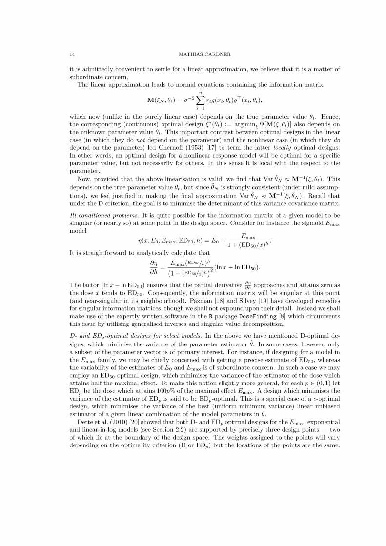
Ill-conditioned problems. It is quite possible for the information matrix of a given model to besingular (or nearly so) at some point in the design space. Consider for instance the sigmoid Emaxmodel


1 + (ED50/x)h .

It is straightforward to analytically calculate that∂η

∂h= Emax(ED50/x)h(

1 + (ED50/x)h)2 (ln x− ln ED50).

The factor (ln x− ln ED50) ensures that the partial derivative ∂η∂h approaches and attains zero as

the dose x tends to ED50. Consequently, the information matrix will be singular at this point(and near-singular in its neighbourhood). Pázman [18] and Silvey [19] have developed remediesfor singular information matrices, though we shall not expound upon their detail. Instead we shallmake use of the expertly written software in the R package DoseFinding [8] which circumventsthis issue by utilising generalised inverses and singular value decomposition.

D- and EDp-optimal designs for select models. In the above we have mentioned D-optimal de-signs, which minimise the variance of the parameter estimator θ. In some cases, however, onlya subset of the parameter vector is of primary interest. For instance, if designing for a model inthe Emax family, we may be chiefly concerned with getting a precise estimate of ED50, whereasthe variability of the estimates of E0 and Emax is of subordinate concern. In such a case we mayemploy an ED50-optimal design, which minimises the variance of the estimator of the dose whichattains half the maximal effect. To make this notion slightly more general, for each p ∈ (0, 1) letEDp be the dose which attains 100p% of the maximal effect Emax. A design which minimises thevariance of the estimator of EDp is said to be EDp-optimal. This is a special case of a c-optimaldesign, which minimises the variance of the best (uniform minimum variance) linear unbiasedestimator of a given linear combination of the model parameters in θ.

Dette et al. (2010) [20] showed that both D- and EDp optimal designs for the Emax, exponentialand linear-in-log models (see Section 2.2) are supported by precisely three design points — twoof which lie at the boundary of the design space. The weights assigned to the points will varydepending on the optimality criterion (D or EDp) but the locations of the points are the same.


It may be surprising that optimal designs for these models include so few dose-levels. Intuitively,we would probably prefer to have more dose-levels, spread out across the design space. Thiswould likely aid assessment of the dose–response profile. However, when designing for a specificmodel, the only consideration is to find the allocation of measurements which is optimal for thatparticular model. Intuition is perhaps more cautious and wary about committing so fully to themodel assumption, which is the topic of the upcoming section.

Efficient designs robust against model misspecifications. As discussed above, optimal designsdepend on the assumption of the underlying model. (This is true for both linear and nonlinearmodels, but in the latter case the design also depends on the model parameters.) Thus a designwhich is optimal for a certain model is generally not optimal for another. As we mentioned in theliterature review (Section 3) Dette et al. (2008) [5] showed that c-optimal designs for commondose–response models are sensitive to misspecifications of the underlying model. In the samearticle, they develop a method for constructing designs which are robust against such modelmisspecifications. Rather than constructing a design which is optimal for any single model, theirmethod yields a design which is appropriate for a collection of candidate models. This collection,which must be specified beforehand by the experimenter, should contain all models likely tocapture the underlying phenomena, but preferably no others.

We shall describe the gist of this method, but all details can be found in the article by Detteet al. (2008) [5]. The benchmark used for judging the aptitude of a given design is its efficiency.Under a general Ψ-criterion of optimality, the Ψ-efficiency of a design ξ is defined by

effΨ(ξ, θ) = Ψ(ξ∗(θ), θ)Ψ(ξ, θ)

where ξ∗(θ) is a locally optimal design (which, being local, depends on the parameter θ). Recallthat the optimal design minimises the functional Ψ, meaning that the efficiency of a given designξ lies between 0 and 1. Say that we under the D-criterion have a design ξ whose efficiencyeffΨ(ξ, θ) = 50%. Then the optimal design ξ∗(θ) would estimate the parameters with the sameprecision as ξ using only half the number of measurements [5]. Alternatively, ξ∗(θ) would yielda more precise confidence region for the parameter estimator θ.

Now, since a locally optimal design depends on the underlying model assumption, so does itsefficiency. Thus, for a given design we must consider its efficiency with respect to each candidatemodel. Dette et al. define a local maximin optimal design to be a design which maximisesthe minimum efficiency across all candidate models. In practice, this design must be foundnumerically, and they have incorporated software for this in the package DoseFinding [8] viathe function optDesign. This software also includes a Bayesian counterpart for constructingadaptive designs under multistage trials. We shall, however, focus on the minimax procedure.Incidentally, the minimax procedure also provides the opportunity to include prior information,namely by weighting the candidate models according to their postulated relevance.

4.2. Nonlinear regression. The function fitMod in the R package DoseFinding [8] is very con-venient for performing nonlinear least-squares regression for common dose–response models. Forinstance, if we have empirical dose–response data stored in the vectors x and Y, respectively, wecan fit an Emax model to the data by calling fitMod(dose = x, resp = Y, model = "emax").This command will return an object whose information can be retrieved using generic R func-tions such as coef (for extracting the estimated model parameters) or vcov (for computing thevariance-covariance matrix of the estimated parameters).

Analogously, we can fit a sigmoid Emax model to the data by calling fitMod(dose = x, resp= Y, model = "sigEmax"). As discussed in Section 2.2 the sigmoid Emax model augments theordinary Emax model by the inclusion of a slope parameter h, which gives the sigmoid model more

16 MATHIAS CARDNER

flexibility. However, this additional parameter (which enters the model in a nonlinear fashion)also makes it more difficult to estimate the parameters of the sigmoid model. An attempt toaddress this issue is to simply fix some of the model parameters; most commonly E0 and Emax.The parameter E0 can be gauged from the vehicle response, since this is indeed a realisation ofthe baseline response. The parameter Emax is not quite as straightforward to estimate, but if weinterpret Emax as the maximum effect seen within the dose-range — as opposed to the maximumeffect as the dose tends to infinity — then this parameter may be sensibly estimated from therange of the observed responses.

The function fitMod does not support fixation of parameters in the regression model. It wouldbe natural to instead use the R function nls to perform nonlinear least squares, but its built-inalgorithms (e.g. Gauss–Newton) often encounter issues of convergence with the sigmoid Emaxmodel. To remedy this, we wish to utilise the Levenberg–Marquardt algorithm, which is morerobust since it mixes the Gauss–Newton algorithm with the method of steepest descent. The Rpackage minpack.lm (where “lm” stands for “Levenberg–Marquardt”) provides this functionality.It is most conveniently utilised via the wrapper function nlsLM whose syntax is very similar tothat of the ordinary nls function, and which supports generic R functions such as coef andvcov. Since nlsLM requires the user to specify the regression model, we are free to fix any of itsparameters. For instance, when fitting a sigmoid Emax model, we may fix E0 and Emax based onprior knowledge (such as a pilot study). This lets the nonlinear regression focus on estimatingED50 and the slope parameter h, which in turn yields more precise parameter estimates — ofcourse at the cost of having fixed some of them.

4.3. Construction of confidence bands. When fitting a regression curve to data, it is im-portant to assess the level of confidence in the fit. The role played by a confidence interval fora single quantity can be extended to a confidence band serving the same purpose for a curve.This concept can most clearly be illustrated in the case of simple linear regression. Suppose thatwe make N observations {(xi, Yi)}Ni=1 under the probabilistic model Yi = β0 + β1xi + εi whoseerrors εi ∼ N (0, σ2) independently. Notice that each xi is considered fixed and that each Yi israndom by virtue of the random error εi. The parameter estimators β0 and β1 of β0 and β1,respectively, are based on ordinary least squares. In Figure 8 we have fitted a regression line toperturbed data generated from the true model y = 2 + 3x. The curved dashed lines constitutea pointwise 95% confidence band around the regression line. It is constructed by computing ateach xi a 95% confidence interval for the fitted value Yi = β0 + β1xi. Then the upper confidencelimits for each fitted value are joined by straight lines in order to outline the upper curve of theconfidence band — and analogously for the lower confidence limits. The curvature is caused bythe fact that an observation Yi at a predictor value xi far from the mean x = 1

N

∑Ni=1 xi will

exert greater leverage on the fitted value Yi, and therefore increase its variance, which in turnwill widen the confidence interval around Yi. More concretely [21] the variance of the ith fittedvalue is

Var Yi =[

1N

+ (xi − x)2∑Nk=1(xk − x)2

]σ2,

where N is the total number of observations. Thus the variance of the ith fitted value Yi increaseswith the distance of xi from the mean x.

It is important to note that confidence bands are intended to capture the fitted values Yi, i.e.the mean profile of the regression curve. It does not give information about the region in whichnew observations are likely to appear. This task is instead fulfilled by prediction bands which arewider than the corresponding confidence bands, due to the increased uncertainty introduced bythe variance of the new observation. For instance, suppose that we wish to predict the responseY ? at some point x?. Since the errors are centred around zero, our best estimate of Y ? is its


●

●

●

●

●

●

●

●

●

●

●

●

●

●

●

●

●

●

● ●

−3 −2 −1 0 1 2 3

−5

05

10

Simple linear regression

x

Y

True modelRegression line

95% confidence band95% prediction band

Figure 8. Simple linear regression with 95% pointwise confidence and predic-tion bands. The confidence band is designed to capture the true model, whichin this case has been accomplished. In contrast, the prediction band is designedto capture the variability of individual observations.

mean Y ? = β0 + β1x?. It can be shown [21] that

Var Y ? =[1 + 1

N+ (x? − x)2∑N

i=1(xi − x)2

]σ2.

In Figure 8 we have constructed a 95% prediction band alongside the 95% confidence band toillustrate this difference. On average, 95% of new observations ought to fall within the widerregion delimited by the prediction band. The confidence band, however, is designed to capture,with some level of confidence, the true model. We say “some level of confidence” because point-wise confidence bands do not in general attain the nominal confidence level of the individualconfidence intervals from which they are constructed, due to the problem of multiple testing [22].

The problem of multiple comparisons. Suppose that we generate a pointwise confidence band byjoining the upper and lower limits of all 100(1 − α)% confidence intervals constructed aroundthe fitted values of N points. Then at each given point, the probability that the correspondingconfidence interval fails to cover the true response is α. However — presuming that the confidenceintervals are independent of each other — the probability that a confidence interval at some pointwill fail to cover the true response (called the family-wise error rate) is FWER = 1− (1− α)N .

18 MATHIAS CARDNER

Writing α = 1 − (1 − α) and noting that (1 − α) < 1 tells us that FWER > α for N > 1. Fortypical values of α and N , the family-wise error rate is dramatically larger than α. For instance,if α = 0.05 and N = 10, then FWER ≈ 40% which is eight times as large as the nominal type Ierror rate of 5%. Admittedly, these computations rely on the assumption of independence,which is violated when fitting a smooth curve since its continuity introduces a dependencystructure between the confidence intervals surrounding the fitted values of neighbouring points.Nevertheless, the coverage level of the pointwise confidence band will generally be lower thanthe nominal confidence level 1 − α of the constituent confidence intervals [22]. To remedy thisproblem, we can attempt to construct simultaneous confidence bands, which are adjusted formultiplicity in order to attain the nominal confidence level. In the upcoming sections we shallinvestigate both approaches.

According to Hall and Horowitz (2013) [23] pointwise confidence bands are, despite theirundercoverage, ubiquitous amongst practitioners and in the literature. In the cited article theypresent a bootstrap method for controlling the asymptotic coverage level of a pointwise confidenceband for a specified proportion of the predictor values. A pointwise confidence band constructedusing their methodology will, in other words, have a 1−α coverage level for a 1−ζ proportion ofthe predictor values, where α and ζ are specified in advance. Their method is a highly compellingalternative to pointwise and simultaneous bands, and it works very well for data whose predictorspace is densely populated. However, since it is based on nonparametric regression via a locallinear estimator, it appears to have difficulties with discrete dose-levels which are separatedby more than the estimated bandwidth. We have tried using both an Epanechnikov kerneland a Gaussian kernel, but to no avail. We also tried appropriating the method for parametricregression (at the risk of violating the assumptions upon which its theoretical foundation depends)but without success. Hence we shall not pursue this method further. Instead, we will focus onconstructing both pointwise and simultaneous confidence bands under normal theory, and also,in the former case, using a bootstrap approach.

First-order Taylor approximation for estimation of variance. In order to construct a confidenceband for a nonlinear function η(x, θ) we must at each point x gauge the variance of η(x, θ). Thuswe consider the predictor point x to be fixed, with all uncertainty about η coming from theparameter estimator. In the present section it is important to distinguish between the parameterθ and its true unknown value, which, as before, is denoted θt.

Following Casella and Berger [24] we let θ = (θ1, . . . , θm)> be a random vector with meanEθ = θt = (θt,1, . . . , θt,m)>. Suppose that η(x, θ) is a real-valued differentiable function. Treatingx as fixed, the first-order Taylor approximation of η about θt is

η(x, θ) ≈ η(x, θt) +m∑i=1

∂η

∂θi(x, θt)(θi − θt,i).

Using vector notation, this can be written as

η(x, θ) ≈ η(x, θt) + (θ − θt)>∂η

∂θ(x, θt), (1)

where ∂η∂θ = ( ∂η∂θ1

, . . . , ∂η∂θm

)> is the gradient of η with respect to θ. Moreover, since E[θi−θt,i] = 0it follows that Eη(x, θ) ≈ η(x, θt). Both of these approximations will be used in the first two


steps of the following derivation of the variance of η at x with respect to θ.

Var η(x, θ) ≈ E[η(x, θ)− η(x, θt)]2 ≈ E[ m∑i=1

∂η

∂θi(x, θt)(θi − θt,i)

]2=

m∑i=1

m∑j=1

∂η

∂θi(x, θt)

∂η

∂θj(x, θt) Cov(θi, θj)

Using matrix notation — and denoting by V the variance-covariance matrix of the random vectorθ — this can be written

Var η(x, θ) ≈ ∂η

∂θ(x, θt)>V∂η

∂θ(x, θt).

This approximation will be utilised in the upcoming section.

Simultaneous confidence bands under normal theory. Gsteiger et al. (2011) [22] describe a methodfor constructing simultaneous confidence bands for nonlinear mixed-effects models under normaltheory. This can easily be applied to our nonlinear fixed-effects model Yij = η(xij , θ) + εij wherewe now add an assumption of normality by supposing that εij ∼ N (0, σ2) independently.

Provided that the maximum likelihood estimate θ is close to the true parameter value θt, theTaylor linearisation in Equation (1) above can be used to yield that

η(x, θ)− η(x, θt) ≈ (θ − θt)>∂η

∂θ(x, θ),

where we have substituted θ for θt in the argument of the gradient ∂η∂θ based on the assumption

of its closeness to the true value θt. The assumption of normality implies that η(x, θ)−η(x, θt) isapproximately N

(0, ∂η∂θ (x, θ)>V∂η

∂θ (x, θ)), where V is the variance-covariance matrix of θ. Thus,

in order to construct a simultaneous confidence band for the curve over the predictor (covariate)region X := [xmin, xmax] we need only calibrate the critical value d so that

P(η(x, θt) ∈ η(x, θ)± d

√∂η

∂θ(x, θ)>V∂η

∂θ(x, θ) : x ∈ X

)= 1− α,

where 1−α is the nominal confidence level and α ∈ (0, 1). Note that setting d to be the (1−α)-quantile of the standard normal distribution yields a pointwise confidence band with confidencelevel (1−α). At first glance it may not be obvious that the variability of the data influences thewidth of the confidence band, but it does so implicitly through the parameter estimate θ and itsvariance-covariance matrix V.

In their paper, Gsteiger et al. describe two methods for determining the critical value d. Thefirst method is based on an asymptotic χ2 distribution, and leads to setting d to the square rootof the (1−α)-quantile of the χ2

m distribution with m degrees of freedom, where m is the numberof parameters in θ. The second method relies on iterated simulation from a multivariate normaldistribution, and it generally yields smaller critical values d than does its approximation-basedcounterpart.

In the same paper, Gsteiger et al. carried out an extensive simulation study in order to assessthe empirical coverage of the confidence bands constructed using critical values determined byeither of the two methods. With α = 0.05 and five distinct dose-levels, they found that theapproximation-based method tends to be conservative for sample sizes larger than 25. In otherwords, the approximation-based confidence bands tend to have an empirical coverage greaterthan the nominal 95% confidence level (of course at the cost of increased width and thereby lessprecision). In contrast, the simulation-based confidence bands generally undercover with respectto the nominal level. Specifically, their empirical coverage ranges (in this study) from 89% to93% for sample sizes between 10 and 50. In summary, the simulation-based method will tend to

20 MATHIAS CARDNER

yield narrower bands which are likely to undercover, whereas the approximation-based methodwill generally yield excessively wide and conservative bands.

Since we will run extensive simulations of dose–response trials, it would be too computationallydemanding to use the simulation-based method for calibrating the critical value d. We havetherefore chosen to use the approximation-based method, which tends to be conservative forlarge sample sizes.

A simple bootstrap method for pointwise confidence bands. The following method is suggested byHastie et al. (2009) [25]. Suppose that we make N observations {(xi, Yi)}Ni=1 and that a modelη(x, θ) is fitted to the data, yielding the parameter estimate θ. Next we compute the residualsεi = Yi − η(xi, θ) and the centred residuals εi = εi − 1

N

∑Ni=1 εi. The latter will be used during

the following bootstrap procedure, which will be iterated for each j ∈ [1, B]∩Z where B > 1000.(1) For i = 1, . . . , N resample Y ∗i = η(xi, θ) + ε∗i where ε∗i is sampled with replacement from

the centred residuals {ε1, . . . , εN}.(2) Fit η(x, θ) to the resampled data, yielding the parameter estimate θ∗j .(3) Save θ∗j .This procedure will yield B curves, each of which has been fitted to some resampling of the

original data. Next we construct a pointwise confidence band by determining empirical (1− α)coverage intervals for each predictor point. In other words, for each x in the predictor regionX := [xmin, xmax] we consider the set {η(x, θ∗j ) : 1 6 j 6 B} of the B fitted values at thatparticular point. The empirical (α/2)- and (1 − α/2)-quantiles of this set are chosen as thelower and upper limits of the confidence band at this point. Notice that this procedure is asimulation-based realisation of the definition of a pointwise confidence band.

Examples. Figure 9 displays a sigmoid Emax model (selected on the basis of Akaike’s informationcriterion) which has been fitted to the dose–response data of compound A with respect to response1. Also included are 95% confidence bands constructed using the methods described above. Thebands based on normal theory are constructed in the same manner, only using different criticalvalues to determine the width of the band. As expected, the simultaneous confidence band iswider than its pointwise counterpart, in order to adjust for multiplicity. It is however encouragingto see that the pointwise confidence band generated using bootstrap agrees rather well with thepointwise confidence band based on normal theory. They deviate most in the regions where theregression curve changes most rapidly, which is where curve fitting is most challenging.

In this case we had no difficulty fitting the regression curve and its confidence band to thedata. However, the sigmoid Emax model can sometimes be difficult to fit for numerical reasons,yielding unwieldy confidence bands which are much too wide to be useful. In such a situationwe can fix some of the model parameters (as described in Section 4.2) in order to get moreprecise estimates of the remaining parameters. Alternatively, we can in such a situation relymore heavily on the confidence bands based on bootstrap, since they suffer no such numericalproblems.


●

●

●

●

●

●

●

●●

●●

●

●

●

●

●

●

●

●

●●

●

●

●

●●●●●●

●

● ●

●

●●●

●●

●●

●

●●●

●●● ●

●

●

●

●●

●

0.5 1.0 2.0 5.0 10.0 20.0 50.0 100.0

050

100

150



Res

pons

e

Regression curve: Sigmoid Emax

Simultaneous 95% confidence band based on normal theoryPointwise 95% confidence band based on normal theoryPointwise 95% confidence band based on bootstrap

Figure 9. Regression curve of a sigmoid Emax model fitted to the dose–responsedata of compound A with respect to response 1. Three 95% confidence bandshave been constructed using the methods described above.

5. Implemented method

We are now ready to address the key question of this thesis, namely the synthesis of an efficacystudy and pharmacodynamic modelling of dose–response data. Concretely, this is attained byusing a simultaneous confidence band around a regression curve (adjusted by subtracting themean vehicle response) to declare whether a given dose in the administered dose-range is active.A dose is said to be active if it shows a statistically significant effect compared to the vehicletreatment (at the given significance level, which in this thesis is set to 5%). It is crucial that weconstruct a confidence band around the difference between the regression curve and the meanvehicle response. Doing so assures that we account for the variability in the former as well asthe latter.Algorithm 1 (Model-based approach to assess efficacy of a given dose). This is the keyresult of this thesis.

(1) Use least-squares regression to fit a model η(x, θ) to dose–response data.(2) Subtract (uniformly) the mean vehicle response V from this curve to yield the difference

η(x, θ)− V .

22 MATHIAS CARDNER

(3) Assuming that the fitted value η(x, θ) and the mean vehicle response V are uncorrelated,the variance of their difference is Var η(x, θ)+Var V . The Taylor approximation in Section4.3 can be used to estimate Var η(x, θ), and an unbiased estimate of Var V is given by

1n(n−1)

∑ni=1(Vi − V )2, where V1, . . . , Vn are the n vehicle responses [24].

(4) Specify a significance level α ∈ (0, 1) and use the method in Section 4.3 to construct asimultaneous 100(1−α)% confidence band around the difference η(x, θ)− V . A commonchoice, used throughout this thesis, is α = 5%.

(5) Declare a given dose x0 to have a significant effect compared to vehicle (at the specifiedsignificance level) if the confidence band around η(x0, θ) − V at this point x0 does notcontain zero.

Figure 10 shows an illustration of the above method, using the empirical dose–response datapertaining to response 1 of compound A. Since the confidence band is adjusted for multiplicity, itis legitimate to use it for simultaneous inference about all doses in the administered dose-range.

●

●

●

●

●

●

●

●●

●●

●

●

●

●

●

●

●

●●

●

●

●

●●●●●●

●

● ●

●

●●●

●●

●●

●

●●●

●●● ●

●

●

●

●●

●

0.5 1.0 2.0 5.0 10.0 20.0 50.0 100.0

050

100

150



Res

pons

e (w

ith m

ean

vehi

cle

resp

onse

sub

trac

ted)

Regression curve: Sigmoid Emax

Simultaneous 95% confidence bandZero responseEstimated minimum active dose: 9

Figure 10. An illustration of the fundamental idea behind judging the activityof doses under the modelling approach. The accuracy of the vehicle-adjustedregression curve is assessed by the dashed confidence band. A dose is deemedactive precisely when the confidence band around its fitted value does not coverthe zero response. In the case shown in this figure, where the lower limit of theconfidence band does not return below zero after first exceeding it, any dosehigher than the estimated minimum active dose is deemed active.


As a comparison, we perform one-way anova on the same data set, and apply Dunnett’s test[6] in order to compare each dose-level against the vehicle treatment. According to this test, onlythe two highest dose-levels, 10 and 100, are deemed active at the 5% significance level. This isin agreement with the conclusion drawn from the modelling approach, since the minimum activedose is estimated to lie between dose-levels 8 and 10. Hence this example is ideal in the sense thatboth methods agree on which of the (discrete) administered dose-levels are active. In addition,the modelling approach provides information about where between the highest inert dose-leveland the lowest active dose-level we begin to see a signal. The reliability of this informationof course depends on the validity of the model assumptions (as we have previously stressed).Nevertheless, this example concretely illustrates the benefit of the quantitative model, whichallows inference to be extended from the administered dose-levels to the entire dose-range. Itis however highly relevant to ask whether the above example is representative of the typicalsituation, and we will address this question via simulations presented in Section 6.1.

24 MATHIAS CARDNER

6. Results and discussion

For each of the empirical data sets described in Section 2, our implemented method fromSection 5 agrees perfectly with Dunnett’s test regarding which dose-levels are active at the 5%significance level. This is encouraging, since we want our method to concur with the authoritativeDunnett’s test on (discrete) administered dose-levels. We will use simulation to investigatewhether this amount of agreement between the two methods is representative.

6.1. Simulations. We shall assess the typical behaviour of the model-based approach (mod)described in Section 5 by simulating dose–response studies. As a frame of reference, we will com-pare the inferences drawn from mod to those made by the multiple comparison procedure (mcp)Dunnett’s test [6]. In order to avoid tailoring the results to a specific scenario, all parameterswill be drawn from probability distributions. We make extensive use of the (scale-parametrised)gamma distribution Γ(k, θ) whose mean is kθ (see e.g. Casella and Berger [24]). In each simulatedtrial, the minimum dose is drawn from Γ(1, 1) with mean 1, and the maximum dose is drawnfrom Γ(11, 13) with mean 143. The desired number of dose-levels are then spaced evenly on alogarithmic scale in this dose-range, and a zero-dose vehicle treatment is included. A total of 40subjects are allotted evenly amongst the groups, and in the case of a remainder, we randomlyselect the dose-levels which receive an additional subject. Recall that the main goal of this thesisis to investigate how the experimental design affects the inferences drawn from mod comparedto those of mcp. Therefore we are interested in the consequences of varying the number ofdose-levels in the simulated trials. However, the total number of subjects is always fixed at 40,in order to prevent this quantity from influencing the results. Consequently, as the number ofdose-levels increases, the number of individuals at each level must decrease.

In the following we will investigate the inferences drawn from the two methods mod andmcp. Concretely, this means that we consider their respective judgements of whether a certaindose-level in a given trial is active (i.e. that it shows a significant effect compared to the vehicletreatment). Since the methods are different in nature, we expect them to disagree some of thetime. For instance, the dose-level under consideration may be declared active by mod but inert(not active) by mcp. A natural way of comparing the methods against each other is to investigatewhich method is more liberal or conservative than the other. By saying, for a certain dose-levelin a given trial, that one method is more liberal than the other, we simply mean that the formerdeclares the given dose-level to be active whereas the latter does not. By conservative we meanthe opposite. It is important to note that this does not mean that the former method is makingan error. Rather, it is merely a way to describe more clearly the disagreement between the twomethods.

Simulations based on the Emax model. In this section we will use the Emax model both to generatedose–response data and to fit a regression curve to the simulated data. The model parametersused for simulation are E0 ∼ Γ(3, 5) and Emax ∼ Γ(5, 7), whilst ED50 is drawn uniformlybetween the minimum and maximum dose. An Emax model with these parameters is employedto generate data, with noise added according to N (0, σ2) where σ = 1

4Emax. (This choice ofstandard deviation is based upon the article by Dette et al. (2008) [5].) A typical simulated trialwill have a minimum dose of 1, a maximum dose of 143, an E0 of 15, an Emax of 35, and an ED50of 72. To each simulated trial, an Emax model is fitted to the perturbed dose–response data, andthe procedure described in Section 5 is performed. In other words, a 95% simultaneous confidenceband is used to determine active doses according to the modelling approach. This judgement iscompared against that made by Dunnett’s test regarding the discrete “administered” dose-levels.

The above procedure is iterated 1000 times, which has been shown to yield high precision inthe results at a reasonable computational expense. In each trial we record which dose-levels are


declared active by mod and mcp, respectively, and average over the 1000 trials to get an estimateof the proportion of dose-levels deemed active by either method. Since we are interested in howthe design affects the results, we run simulations with the total number of dose-levels (includingthe vehicle group) ranging from 3 through 10. The results are displayed in Figure 11.

●

●

●● ● ● ●

●

3 4 5 6 7 8 9 10

020

4060

8010

0

Proportion of dose−levels deemed active

Number of dose−levels

Pro

port

ion

of d

ose−

leve

ls d

eem

ed a

ctiv

e (%

)

●

●

●●

●●

●

●

Active dose−levels according to MODActive dose−levels according to MCP

Figure 11. Proportion of dose-levels declared active at the 95% significancelevel by the modelling approach (mod) and the multiple comparison procedure(mcp). Each estimate is based on 1000 simulated dose–response trials with theindicated number of dose-levels. Since the total number of subjects is fixed (at40), the number of individuals per dose-level must decrease as the number ofdose-levels increases.

We find that mod tends to be more conservative than mcp in designs with fewer than sixdose-levels, but that this relationship is reversed in designs with more than six dose-levels.

Simulations with model misspecification. In order to assess the consequences of misspecifyingthe underlying model we now simulate trials from a sigmoid Emax model, but fit an ordinary(hyperbolic) Emax model to the data. The parameters for data generation follow the samedistributions as before, with the addition of the slope parameter h ∼ N (0, 32). This distributionof h has been chosen in order to yield slope parameters which are spread quite far from ±1,since the models coincide in those cases. Figure 12 shows the results of 1000 such simulatedtrials. Note that mcp does not include any assumption of the underlying dose–response model,wherefore it is unaffected by its misspecification. Thus the dashed line pertaining to mcp canbe used as a reference for comparison with simulations under a valid model assumption, shownin Figure 11 above.

26 MATHIAS CARDNER

●

●●

● ●

● ●●

3 4 5 6 7 8 9 10

020

4060

8010

0


Number of dose−levels

Pro

port

ion

of d

ose−

leve

ls d

eem

ed a

ctiv

e (%

)

●

●

●

●●

●● ●


Figure 12. Proportion of dose-levels declared active at the 95% significancelevel by mcp and mod under model misspecification. Each estimate is based on1000 simulated dose–response trials with the indicated number of dose-levels.Since the total number of subjects is fixed (at 40), the number of individualsper dose-level must decrease as the number of dose-levels increases.

Simulating optimal designs. Consider that mod is most liberal when its confidence band is asnarrow as possible (since such a band is most prone not to cover the zero response). This occurswhen the parameter estimates are as precise as possible, which they are in a D-optimal design. Inorder to connect optimal design to comparisons between mod and mcp, we will now investigatethe consequences of optimally designing the simulated trials. Thus we modify the procedureabove by allocating dose-levels and their sample sizes in a D-optimal fashion. We shall let ourmodel assumption be valid in these simulations, and use an Emax model both for data generationand regression. More concretely, we use the function optDesign of the R package DoseFinding[8] to choose a D-optimal design for the Emax model. However, this function requires that wesupply a collection of candidate dose-levels, amongst which optDesign determines the mostefficient allocation. Hence optDesign will never suggest a dose-level not included amongst thecandidates. Rather, it will return the optimal allocation of observations across the candidatedose-levels, some of which may well be assigned a zero weight, thereby excluding them from thedesign. As we shall see momentarily, this will generally lead to a discrepancy between the nominaland the actual number of dose-levels of an optimal design. The nominal number is simply thenumber of candidate dose-levels, whereas the actual number is the number of dose-levels selectedby optDesign.

For each (nominal) number of dose-levels (3, 4, . . . , 10) we simulate 1000 dose–response datasets from an Emax model as in the previous section. In each such trial, we let the candidatedose-levels be spread out evenly on a logarithmic scale. The actual dose-levels, chosen amongst


these candidates, are then used when simulating a dose–response trial. The verdicts of mod andmcp, respectively, are displayed in Figure 13.

●

● ●

●●

●●

●

3 4 5 6 7 8 9 10

020

4060

8010

0


NOMINAL number of dose−levels

Pro

port

ion

of d

ose−

leve

ls d

eem

ed a

ctiv

e (%

)

●

●●

●

●

●●

●


Figure 13. Proportion of dose-levels declared active at the 95% significancelevel by mod and mcp. Each estimate is based on 1000 simulated dose–responsetrials which have been D-optimally designed with a valid Emax model assump-tion. It is important to note that the number of dose-levels are nominal — notactual. In fact, the true number of dose-levels is almost always 3.

See Section 7 for our conclusions about all the above results.

28 MATHIAS CARDNER

6.2. White book. In this section we shall describe how to use the methods in the R [7] packageDoseFinding [8] for design and analysis of dose–response experiments. This software supports theD-criterion of optimality, which maximises the precision of the estimated model parameters. Italso offers support to make the design optimal for estimating the minimum effective dose (MED)defined as the smallest dose which yields a clinically relevant and statistically significant effect [4].A design which is optimal in the latter sense is said to be MED-optimal. It is important to notethat the clinically relevant effect ∆ must be specified by an expert before the statistical analysisis performed. For instance, an experimenter might only be interested in whether a compound canincrease the response by at least ∆ = 0.4 units over the vehicle response — regardless of whethera smaller effect is found to be statistically significant. It is of course possible that no clinicallyrelevant effect exists — and also that it does but without being detectable due to high variabilityin the measurements or insufficient sample size [1]. However, it is only the MED-optimal designwhich actually requires ∆ to be specified. The D-optimal design operates without it, since itsonly objective is to minimise the variance of the estimator of the model parameters.Algorithm 2 (Robust optimal design of a dose–response experiment). The following functionsare contained in the R package DoseFinding [8] whose help pages offer more detailed information.

(1) Nominate the candidate models which are conjectured to capture the true dose–responserelationship. Only include models which are likely to be relevant, and rank each modelwith a probability corresponding to your belief that it most aptly describes the underlyingrelationship. These probabilities must sum to unity, and in the absence of prior knowledgethey may be set to 1/m, where m is the number of candidate models. Notice that theparameters of the nonlinear part of each model must be (numerically) specified.

(2) Suggest a collection of feasible dose-levels. The recommended dose-levels will be chosenamongst this set, though allocated in an optimal way.

(3) Use optDesign to compute the optimal dose-levels and their corresponding weights.Use rndDesign to efficiently round the optimal design to attain an integer number ofmeasurements (possibly zero) to be made at each dose-level.

Algorithm 3 (Analysis of a dose–response experiment). The following functions are containedin the R package DoseFinding [8] whose help pages offer more detailed information.

(1) Fit each candidate model (from Algorithm 2) to the empirical data using fitMod.(2) Use MCPMod to determine which model (fitted in the previous step) most aptly describes

the empirical data. If there are few active dose-levels, or if the models are highly corre-lated (and thus difficult to distinguish), MCPMod may fail to identify the most appropriatemodel. If so, model selection can for instance be based on Akaike’s information criterion.Use the winning model for all further analysis and inference.

(3) Use the method in Section 5 to construct a simultaneous confidence band around thevehicle-adjusted regression curve of the winning model. A dose is declared to yield asignificant effect compared to vehicle if and only if the confidence band around its fittedresponse does not cover zero.


7. Conclusions

In this thesis we implement a method for assessing efficacy in a model-based setting (seeSection 5). This method is based on constructing a confidence band around a vehicle-adjustedregression curve fitted to dose–response data. We declare a dose to be active if and only ifthe confidence band at its fitted value does not cover zero. A dose-level is said to be active if itshows a statistically significant effect compared to the vehicle treatment (at the given significancelevel, which in this thesis is set to 5%). In order to evaluate the inferential properties of thismethod, we simulate dose–response trials in which its conclusions are compared to those ofanova coupled with Dunnett’s multiple comparison procedure. We consider the latter to be anauthoritative benchmark regarding which of the (discrete) administered dose-levels are active ina given trial. The main advantage of the model-based procedure is its capacity to declare activity(on a continuous scale) in between administered dose-levels. We find that to a large extent, thetwo methods draw similar inferences concerning administered dose-levels. There are howeversystematic discrepancies, which may be elucidated by considering the nature of either method.

When comparing our model-based implementation (mod) to anova coupled with Dunnett’smultiple comparison procedure, we find that the former tends to be more conservative relativeto the latter in designs with fewer than six logarithmically spaced dose-levels, but that theconverse is true in designs with more than six logarithmically spaced dose-levels. These resultsare displayed in Figure 11. This makes sense intuitively, because a design with few dose-levelsand many individuals per level benefits Dunnett’s test, since there are few comparisons for whichto adjust and many subjects per group to gain high precision. However, it is not ideal for theregression and confidence band in mod, which rather benefit from a larger number of dose-levels spread out across the dose-range. This is more advantageous for curve fitting, giving moreprecision in the estimated parameters. In turn, this yields narrower confidence bands, whichare more likely not to contain zero. It should be noted that both methods are punished as thenumber of dose-levels increases. In the case of Dunnett’s test, this is because the procedure hasto adjust for more comparisons with fewer individuals per dose-level, which yields less statisticalconfidence at each level, thereby raising the bar for detecting a signal. In the case of mod it isbecause the estimate of the mean vehicle response becomes more variable as the vehicle group isreduced, which yields wider, more conservative, confidence bands.

In order to investigate the effect of misspecifying the underlying dose–response model, wesimulate trials in which we fit an ordinary Emax model to data generated by a sigmoid Emaxmodel. The results are displayed in Figure 12. We see no systematic effect of this modelmisspecification on the proportion of dose-levels deemed active by the model-based procedure.

Now consider that mod is most liberal when its confidence band is as narrow as possible(since such a band is most prone not to cover the zero response). This occurs when the parameterestimates are as precise as possible, which they are in a D-optimal design. Increasing the numberof dose-levels cannot yield narrower confidence bands than those of a D-optimal design. Whenoptimally designing the simulated trials with a valid Emax model assumption, both methods aredramatically more prone to declare dose-levels active. These results are displayed in Figure 13.In the case of mod, the leap in declarations of activity between three and four nominal dose-levelsmay at its root be caused by the fact that a larger nominal number of dose-levels will yield afiner, more densely spaced set of candidate dose-levels. As a result, the design algorithm will beable to choose dose-levels closer to those of the true D-optimal design, which will yield higherprecision in the parameter estimates. This in turn will lead to narrower confidence bands, which,finally, yield more liberal judgements of activity. However, we witness a virtually identical leapin declarations of activity by Dunnett’s test, which may well benefit from a more carefully chosendesign, but on which the remaining chain of events has no bearing.

30 MATHIAS CARDNER

At first glance, it may also appear that optimally designing the simulated trials eliminatesthe previously observed trend that declarations of activity decrease as the nominal number ofdose-levels increases. This is however an illusion, caused by the fact that the design algorithmgenerally selects only three dose-levels, irrespective of the nominal number of candidate dose-levels with which it is provided. As mentioned in Section 4.1, this can be shown [20] to bethe correct number of dose-levels for any D-optimal design under the Emax model. A naturalcontinuation of these investigations would be to combine model misspecification with optimaldesign. Moreover, this offers an opportunity to assess model-robustness, namely by includingseveral candidate models and utilising the model-robust optimal designs described in Section 6.2of this thesis.

Future work. Our model-based method (Section 5) is designed to detect doses which show asignificant effect compared to the vehicle treatment. However, as mentioned in Section 3, it mayalso be of interest to compare the compound under investigation against a reference treatment(e.g. a competing compound). Dette et al. (2014) [14] have developed optimal designs for suchstudies, and their work may serve as a source of inspiration for ideas of how to appropriate ourmethod to accommodate this scenario.

When implementing our method in Section 5 we made the assumption that the fitted values ofthe regression curve and the mean vehicle response are uncorrelated. This may not be valid, sincethe vehicle responses are used during regression. Investigating this correlation would perhapsyield more faithful results. However, the pointwise confidence bands generated by the bootstrapagree quite well with those constructed under this assumption, which indicates that it may beof subordinate concern. On a related note, when estimating the variance of the mean vehicleresponse, we do not use the pooled sample variance across all dose-levels. This may be advisablein a heteroscedastic case, but in a homoscedastic case, doing so would likely yield a betterestimate.

In this thesis we have only mentioned Dunnett’s test as a benchmark against which to compareour modelling approach. This is because Dunnett’s test is designed to compare the responseof each dose-level to that of the vehicle treatment, which is the qualitative analogue of whatwe do when checking whether the confidence band contains the zero response. There are ofcourse other multiple comparison procedures which may be appropriate, and we have for instanceexperimented with Williams’ trend test. This is designed to test for a monotonic dose–responseprofile, and it involves borrowing strength from neighbouring dose-levels in order to do so. Itcould be argued that this is a more appropriate analogue to our modelling approach, since ourcandidate regression models are (all but one) monotonic. However, we do not use our modellingprocedure to test for the existence of a trend. For instance, even though the regression curve isconstricted to be monotonic, its confidence band is not. If the parameter estimates are highlyvariable, a dose may be inert even though it is higher than the minimum active dose. In thecase of an increasing dose–response profile, this occurs when the lower limit of the confidenceband returns below the zero response after first having exceeded it. As mentioned above, this isbecause we are investigating individual dose-levels rather than the existence of a trend, which isthe reason for our preference of Dunnett’s test. Nevertheless, it would be a natural continuationof our work to extend the model-based procedure to test for the existence of a monotonic dose–response trend. If for instance the confidence band around the smallest (non-vehicle) dose doesnot overlap with that around the largest dose, then we would be confident that a dose–responsetrend exists. However, this is almost certainly an excessively cautious criterion, but it is notobvious how to moderate it whilst still retaining confidence in the result. Doing so may wellpresent a stimulating challenge.


References[1] F. Bretz, J. C. Pinheiro, and M. Branson, “Combining multiple comparisons and modeling techniques in

dose–response studies,” Biometrics, vol. 61, no. 3, pp. 738–748, 2005.[2] J. Pinheiro, B. Bornkamp, and F. Bretz, “Design and analysis of dose-finding studies combining multiple

comparisons and modeling procedures,” Journal of Biopharmaceutical Statistics, vol. 16, no. 5, pp. 639–656,2006.

[3] F. Bretz, H. Dette, and J. C. Pinheiro, “Practical considerations for optimal designs in clinical dose findingstudies,” Statistics in Medicine, vol. 29, no. 7-8, pp. 731–742, 2010.

[4] S. J. Ruberg, “Dose response studies I. Some design considerations,” Journal of Biopharmaceutical Statistics,vol. 5, no. 1, pp. 1–14, 1995.

[5] H. Dette, F. Bretz, A. Pepelyshev, and J. Pinheiro, “Optimal designs for dose-finding studies,” Journal ofthe American Statistical Association, vol. 103, no. 483, pp. 1225–1237, 2008.

[6] F. Bretz, T. Hothorn, and P. Westfall, Multiple comparisons using R. CRC Press, 2010.[7] R Core Team, R: A Language and Environment for Statistical Computing. R Foundation for Statistical

Computing, Vienna, Austria, 2014.[8] B. Bornkamp, J. Pinheiro, and F. Bretz, DoseFinding: planning and analyzing dose finding experiments,

2014. R package version 0.9-12.[9] T. Hothorn, F. Bretz, and P. Westfall, “Simultaneous inference in general parametric models,” Biometrical

Journal, vol. 50, no. 3, pp. 346–363, 2008.[10] J. Macdougall, “Analysis of dose–response studies—Emax model,” in Dose Finding in Drug Development

(N. Ting, ed.), Statistics for Biology and Health, pp. 127–145, Springer New York, 2006.[11] J. Gabrielsson and D. Weiner, Pharmacokinetic & Pharmacodynamic Data Analysis: Concepts and Appli-

cations. Stockholm: Swedish Academy of Pharmaceutical Sciences, 4th ed., 2006.[12] V. V. Fedorov and S. L. Leonov, Optimal Design for Nonlinear Response Models. Chapman & Hall/CRC

Biostatistics Series, Taylor & Francis, 2013.[13] B. Bornkamp, J. Pinheiro, and F. Bretz, “MCPMod: An R package for the design and analysis of dose-finding

studies,” Journal of Statistical Software, vol. 29, no. 7, pp. 1–23, 2009.[14] H. Dette, C. Kiss, N. Benda, and F. Bretz, “Optimal designs for dose finding studies with an active control,”

Journal of the Royal Statistical Society: Series B (Statistical Methodology), vol. 76, no. 1, pp. 265–295, 2014.[15] A. C. Atkinson, A. N. Donev, and R. Tobias, Optimum Experimental Designs, with SAS. Oxford statistical

science series, Oxford University Press, 2007.[16] V. Fedorov, “Optimal experimental design,” Wiley Interdisciplinary Reviews: Computational Statistics,

vol. 2, no. 5, pp. 581–589, 2010.[17] H. Chernoff, “Locally optimal designs for estimating parameters,” The Annals of Mathematical Statistics,

pp. 586–602, 1953.[18] A. Pázman, “Computation of the optimum designs under singular information matrices,” The Annals of

Statistics, vol. 6, no. 2, pp. 465–467, 1978.[19] S. D. Silvey, “Optimal design measures with singular information matrices,” Biometrika, vol. 65, no. 3,

pp. 553–559, 1978.[20] H. Dette, C. Kiss, M. Bevanda, and F. Bretz, “Optimal designs for the Emax, log-linear and exponential

models,” Biometrika, vol. 97, no. 2, pp. 513–518, 2010.[21] J. O. Rawlings, S. G. Pantula, and D. A. Dickey, Applied Regression Analysis: A Research Tool. Springer

Texts in Statistics, Springer, 2nd ed., 1998.[22] S. Gsteiger, F. Bretz, and W. Liu, “Simultaneous confidence bands for nonlinear regression models with

application to population pharmacokinetic analyses,” Journal of Biopharmaceutical Statistics, vol. 21, no. 4,pp. 708–725, 2011.

[23] P. Hall and J. Horowitz, “A simple bootstrap method for constructing nonparametric confidence bands forfunctions,” The Annals of Statistics, vol. 41, no. 4, pp. 1892–1921, 2013.

[24] G. Casella and R. L. Berger, Statistical Inference. Pacific Grove, California: Duxbury, 2nd ed., 2002.[25] T. Hastie, R. Tibshirani, and J. Friedman, The Elements of Statistical Learning. Stanford, California:

Springer, 2nd ed., 2009.

curve fitting with confidence for preclinical dose

Documents